Simulation and stability analysis of oblique shock wave/boundary
layer interactions at Mach 5.92

Abstract

We investigate flow instability created by an oblique shock wave impinging on a Mach 5.92 laminar boundary layer at a transitional Reynolds number. The adverse pressure gradient of the oblique shock causes the boundary layer to separate from the wall, resulting in the formation of a recirculation bubble. For sufficiently large oblique shock angles, the recirculation bubble is unstable to three-dimensional perturbations and the flow bifurcates from its original laminar state. We utilize Direct Numerical Simulation (DNS) and Global Stability Analysis (GSA) to show that this first occurs at a critical shock angle of $\theta=12.9\degree$. At bifurcation, the least stable global mode is non-oscillatory, and it takes place at a spanwise wavenumber $\beta=0.25$, in good agreement with DNS results. Examination of the critical global mode reveals that it originates from an interaction between small spanwise corrugations at the base of the incident shock, streamwise vortices inside the recirculation bubble, and spanwise modulation of the bubble strength. The global mode drives the formation of long streamwise streaks downstream of the bubble. While the streaks may be amplified by either the lift-up effect or by Görtler instability, we show that centrifugal instability plays no role in the upstream self-sustaining mechanism of the global mode. We employ an adjoint solver to corroborate our physical interpretation by showing that the critical global mode is most sensitive to base flow modifications that are entirely contained inside the recirculation bubble.

I INTRODUCTION

High-speed flows over complex geometries are typically characterized by shock wave/boundary layer interactions (SWBLI). Sudden changes in geometry such as compression ramps or the leading edges of fins create shock waves that propagate over large distances. When a shock wave comes into contact with a boundary layer flow, the large adverse pressure gradient associated with the shock wave can cause the flow to separate from the surface. When this happens, a recirculation bubble forms close to the wall, and significantly alters the stability and dynamics of the flow. In some cases, this interaction can cause an otherwise laminar flow to prematurely transition to turbulence. Transition to turbulence is accompanied by a five-to-six fold increase in heat flux to the wall White . For this reason, the performance of a hypersonic vehicle often depends upon delaying transition to turbulence as much as possible. Unfortunately, fundamental understanding of shock-induced boundary layer transition is still lacking.

While there have been many experimental and numerical investigations of shock waves interacting with both laminar Pagella ; Benay ; Robinet ; Sandham ; Guiho ; Gs and turbulent Unalmis ; Ganapath ; Wu ; Delery ; Touber ; Nichols3 ; Priebe ; Dupont ; Piponniau ; Pirozzoli ; Sansica ; Clemens boundary layers, studies of shock waves interacting with boundary layers at transitional Reynolds numbers are relatively sparse. Interactions with hypersonic boundary layers at transitional Reynolds numbers can produce complex and unexpected behavior. For example, recent experiments of hypersonic boundary layer flow past cylindrical posts remain well-behaved if the incoming boundary layer is either laminar or fully turbulent, but show complex behavior if the boundary layer is in a transitional state Murphree ; Lash . In the experiment, the cylindrical posts create complicated interactions between bow shocks and recirculation bubbles. In this paper, however, we focus instead upon the simpler configuration of an oblique shock wave impinging on a flat plate hypersonic boundary layer at a transitional Reynolds number. This oblique shock wave configuration has been recently investigated experimentally and numerically in Sandham . Their experiments and simulations introduced varying levels of forcing into the Mach 6 boundary layer upstream of the impinging shock. They observed the shock to amplify second (Mack) mode instabilities Mack ; Federov downstream. The interaction of second mode instability with boundary layer streaks was thought to precipitate transition. It is conceivable, however, that a recirculation bubble can support self-sustaining instability, even in the absence of upstream forcing. This was observed, for example, by Robinet for a shock wave/laminar boundary layer interaction at Mach 2.15 Robinet . The aim of the present study, therefore, is to assess whether self-sustaining instability can play a role in transitional shock wave/boundary interactions at Mach 5.92, and to understand the physical mechanisms underlying such instability.

We investigate transitional shock wave/boundary layer interaction with direct numerical simulation (DNS) and global stability analysis (GSA). In this regard, our approach is conceptually similar to that of Robinet Robinet , but increased computational power available today enables an investigation at a transitional Reynolds number and higher Mach number. As we will see, these flow conditions accentuate different flow features that result in a new fluid mechanical model of the physical mechanism responsible for the instability. In particular, because streamlines curve around the recirculation bubble, we investigate centrifugal instability as a possible mechanism for SWBLI instability Priebe . We apply the massively parallel hypersonic flow solver US3D Candler to perform DNS of SWBLI in domains of large spanwise extent to revisit the question of whether the bifurcation of a shock wave/boundary layer interaction to self-sustaining instability is stationary or oscillatory (previous DNS produced inconclusive results Robinet ). We also extend the global stability analysis to include adjoint mode analysis. Adjoint global modes show how SWBLI instability can be optimally triggered, and provide information about the sensitivity of direct global modes to changes in the base flow. This provides additional insight into the mechanism responsible for SWBLI instability.

II PROBLEM FORMULATION

II.1 Flow configuration

Figure 1 shows a schematic of a canonical SWBLI that we consider in this study. High-speed freestream flow enters at the left boundary, and flows over a flat plate situated along the bottom edge of the domain. The leading edge of the flat plate is assumed to be upstream of the left boundary. Nevertheless, the leading edge produces a bow shock which enters the domain through the left boundary, as shown. We will discuss precisely how we calculate this in a later section, below. At the inlet, the boundary layer has displacement thickness $\delta^{*}$, and slowly grows as it develops downstream. Also, an oblique shock wave enters the domain through the left boundary well above both the boundary layer and bow shock. Such an oblique shock wave might result from placing a turning wedge in the freestream a distance upstream. The incident oblique shock wave propagates at angle $\theta$ until it impinges on the boundary layer. The adverse pressure gradient of the impinging shock causes the boundary layer to separate from the wall and form a recirculation bubble. Because of recirculation, the boundary layer separation point is well upstream of the impingement point. The recirculation bubble displaces flow, and causes it to bend around it. Concave streamline curvature on the upstream and downstream portions of the bubble creates compression waves, which at high Mach number quickly coalesce into separation and reattachment reflected shock waves. Convex streamline curvature as the flow passes over the bubble top leads to an expansion fan in between these two reflected shocks.

We consider freestream flow conditions matching experiments performed in the ACE Hypersonic Wind Tunnel at Texas A&M University Semper . Between the bow shock and incident shock, the freestream Mach number, temperature, and pressure are $M_{\infty}=5.92$, $T_{\infty}=53.06$ K, and $p_{\infty}=308.2$ Pa, respectively. A Reynolds number of $Re=\rho_{\infty}U_{\infty}\delta^{*}/\mu_{\infty}=9660$ based on the undisturbed boundary layer displacement thickness $\delta^{*}=2.1$mm at the inlet is used in the present study. This corresponds to a unit Reynolds number of $4.6\times 10^{6}$ m^-1. Here, $\rho_{\infty}$, $U_{\infty}$, and $\mu_{\infty}$ denote the freestream density, velocity, and dynamic viscosity, respectively. We consider incident shock angles ranging from 12.6 to 13.6 degrees. As the shock angle increases, the strength of the SWBLI increases. In particular, the adverse pressure gradient becomes larger, leading to earlier boundary layer separation and larger recirculation bubbles. A Cartesian coordinate system is utilized hereafter with $x$, $y$, and $z$ denoting the streamwise, wall-normal, and spanwise directions, respectively.

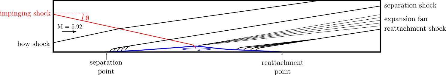
Figure 1: A schematic of an oblique shock wave (red) impinging on a Mach 5.92 boundary layer. The adverse pressure gradient associated with the impinging shock causes the boundary layer to separate from the wall, forming a recirculation bubble (blue).

II.2 Governing equations

The compressible Navier-Stokes equations are used to mathematically model the dynamics of an oblique shock wave/laminar boundary layer interaction at hypersonic speeds. These equations govern the evolution of the system state $\bm{q}=[p;\hskip 2.84544pt\bm{u}^{\mathrm{T}};\hskip 2.84544pts]^{\mathrm{T}}$, where $p$, $\bm{u}$, and $s$ are the non-dimensional fluid pressure, velocity, and entropy, respectively [Sesterhenn, ,Nichols, ]. After non-dimensionalization with respect to the displacement thickness $\delta^{*}$, freestream velocity $U_{\infty}$, density $\rho_{\infty}$, and temperature $T_{\infty}$, these equations are written as

$$\frac{\partial{p}}{\partial{t}}+\bm{u\cdot\nabla}p+\rho{c^{2}}\bm{\nabla\cdot{u}}=\frac{1}{Re}\bigg{[}\frac{1}{M_{\infty}^{2}Pr}\bm{\nabla\cdot}(\mu\bm{\nabla}T)+(\gamma-1)\phi\bigg{]},$$ (1a)

$$\frac{\partial\bm{u}}{\partial{t}}+\frac{1}{\rho}\bm{\nabla}p+\bm{u\cdot\nabla{u}}=\frac{1}{Re}\frac{1}{\rho}\bm{\nabla\cdot\uptau},$$ (1b)

$$\frac{\partial{s}}{\partial{t}}+\bm{u\cdot\nabla}s=\frac{1}{Re}\frac{1}{\rho{T}}\bigg{[}\frac{1}{(\gamma-1)M_{\infty}^{2}Pr}\bm{\nabla\cdot}(\mu\bm{\nabla}T)+\phi\bigg{]}.$$ (1c)

The time scales are normalized by $\delta^{*}/U_{\infty}$ and pressure with $\rho_{\infty}{U^{2}_{\infty}}$. For an ideal fluid, the density $\rho$ and temperature $T$ are related to pressure $p$ through the equation of state $\gamma{M_{\infty}^{2}}p=\rho{T}$. The freestream Mach number is defined as $M_{\infty}=U_{\infty}/a_{\infty}$, where $a_{\infty}=\sqrt{\gamma{p_{\infty}/}\rho_{\infty}}$ is the speed of sound in the freestream. Furthermore, $\gamma=1.4$ is the assumed constant ratio of specific heats.

For the present study, entropy is defined as $s=\ln(T)/[(\gamma-1)M_{\infty}^{2}]-\ln(p)/(\gamma{M_{\infty}^{2}})$ so that $s=0$ when $p=1$ and $T=1$. The viscous stress tensor $\bm{\uptau}$ is written in terms of the identity matrix $\bm{I}$, velocity vector $\bm{u}$, and dynamic viscosity $\mu$ to yield the following expression

$$\bm{\uptau}=\mu[\bm{\nabla{u}}+(\bm{\nabla{u}})^{\mathrm{T}}-\frac{2}{3}(\bm{\nabla\cdot{u}})\bm{I}].$$ (2)

The viscous dissipation is defined as $\phi=\bm{\uptau:\nabla{u}}$. Note the operator $\bm{:}$ represents a scalar or double dot product between two tensors. Furthermore, the second viscosity coefficient is set to $\lambda=-2\mu/3$. In order to compute the dynamic viscosity $\mu$, Sutherland’s law is used with $T_{s}=110.3~{}\mathrm{K}$ as follows

$$\mu(T)=T^{3/2}\frac{1+T_{s}/T_{\infty}}{T+T_{s}/T_{\infty}}.\vspace{0.2cm}$$ (3)

The Prandtl number is set to a constant value $Pr=\mu(T)/\kappa(T)=0.72$, where $\kappa(T)$ is the coefficient of heat conductivity.

II.3 Linearized model

To investigate the behavior of small fluctuations about various base flows, system (1c) is linearized by decomposing the state variables $\bm{q}=\bar{\bm{q}}+\bm{q}^{\prime}$ into steady and fluctuating parts. By keeping only the first-order terms in $\bm{q}^{\prime}$, the Linearized Navier-Stokes (LNS) equations are obtained

$$\begin{split}\frac{\partial{p^{\prime}}}{\partial{t}}+\bar{\bm{u}}\bm{\cdot\nabla}p^{\prime}+\bm{u}^{\prime}\bm{\cdot\nabla}\bar{p}\hskip 1.42271pt&+\bar{\rho}\bar{c}^{2}\bm{\nabla\cdot{u}}^{\prime}+\gamma(\bm{\nabla\cdot}\bar{\bm{u}})p^{\prime}=\frac{1}{Re}\bigg{\{}\frac{1}{M_{\infty}^{2}Pr}\bm{\nabla\cdot}(\bar{\mu}\bm{\nabla}T^{\prime})\\[-17.22217pt] \\ &+(\gamma-1)\big{[}\bar{\bm{\uptau}}\bm{:\nabla{u}}^{\prime}+\bm{\uptau}^{\prime}\bm{:\nabla}\bar{\bm{u}}\big{]}\bigg{\}},\end{split}$$ (4a)

$$\frac{\partial\bm{u}^{\prime}}{\partial{t}}+\frac{1}{\bar{\rho}}\bm{\nabla}p^{\prime}-\frac{\rho^{\prime}}{\bar{\rho}^{2}}\bm{\nabla}\bar{p}+\bar{\bm{u}}\bm{\cdot\nabla{u}}^{\prime}+\bm{u}^{\prime}\bm{\cdot\nabla}\bar{\bm{u}}=\frac{1}{Re}\bigg{\{}\frac{1}{\bar{\rho}}\bm{\nabla\cdot\uptau}^{\prime}-\frac{\rho^{\prime}}{\bar{\rho}^{2}}\bm{\nabla\cdot}\bar{\bm{\uptau}}\bigg{\}},$$ (4b)

$$\begin{split}\frac{\partial{s^{\prime}}}{\partial{t}}+\bar{\bm{u}}\bm{\cdot\nabla}s^{\prime}+\bm{u}^{\prime}\bm{\cdot\nabla}\bar{s}\hskip 1.42271pt&=\frac{1}{Re}\frac{1}{\bar{\rho}\overline{T}}\bigg{\{}\frac{1}{(\gamma-1)M_{\infty}^{2}Pr}\bigg{[}\bm{\nabla\cdot}(\bar{\mu}\bm{\nabla}T^{\prime})-\frac{p^{\prime}}{\bar{p}}\bm{\nabla\cdot}(\bar{\mu}\bm{\nabla}\bar{T})\bigg{]}\\[-17.22217pt] \\ &+\bar{\bm{\uptau}}\bm{:\nabla{u}}^{\prime}+\bm{\uptau}^{\prime}\bm{:\nabla}\bar{\bm{u}}-\frac{p^{\prime}}{\bar{p}}\bar{\bm{\uptau}}\bm{:\nabla}\bar{\bm{u}}\bigg{\}}.\end{split}$$ (4c)

The overbars and primes denote the base flow and fluctuating parts, respectively. Moreover, the equation of state is linearized to obtain $\rho^{\prime}/\bar{\rho}=p^{\prime}/\bar{p}-T^{\prime}/\bar{T}$. The expression $T^{\prime}=(\gamma-1)M_{\infty}^{2}(\bar{T}s^{\prime}+p^{\prime}/\bar{\rho})$ is derived by linearizing the definition of entropy and substituting in the equation of state. In Appendix A, we verify the accuracy of our global mode solver by applying it to a range of known test cases involving high-speed boundary layers at flow conditions similar to those of our SWBLI, but without shocks.

Global modes of the linear system (4c) take the form

$$\bm{q}^{\prime}(x,y,z,t)=\hat{\bm{q}}(x,y)e^{i(\beta{z}-\omega{t})},$$ (5)

where $\beta$ is the non-dimensional spanwise wavenumber and $\omega$ is the temporal frequency. Substitution of (5) into system (4c) yields the eigenvalue problem

$$A\hat{\bm{q}}=-i\omega\hat{\bm{q}}.$$ (6)

The operator $A$, known as the Jacobian operator, involves all terms in system (4c) that do not involve a time derivative. The Jacobian operator gives the linear variation of the residual (i.e., terms without a time derivative) of the original nonlinear system (1c) with respect to the state variables, taken about a base flow.

II.4 Numerical methods

For the base flow calculations and direct numerical simulations, the compressible Navier-Stokes equations are solved in conservative form Shrestha . A stable, low-dissipation scheme based upon the Kinetic Energy Consistent (KEC) method developed by Subbareddy and Candler Subbareddy is implemented for the inviscid flux computation. In this numerical method, the flux is split into a symmetric (or non-dissipative) portion and an upwind (or dissipative) portion. The inviscid flux is pre-multiplied by a shock-detecting switch, which ensures that dissipation occurs only around shocks Ducros . A sixth-order, centered KEC scheme is employed for the present study. Viscous fluxes are modeled with second-order, central differences. Time integration is performed using an implicit, second-order Euler method with point relaxation to maintain numerical stability Wright . The implicit system is solved using the full matrix Data Parallel Line Relaxation (DPLR) method, which has good parallel efficiency Wright2 .

For the stability analysis, the linear system of equations (4c) are discretized by fourth-order, centered finite differences applied on a stretched mesh. This results in a large, sparse matrix Nichols . Global modes are extracted by the shift-and-invert Arnoldi method implemented by the software package ARPACK Lehoucq . The inversion step is computed by finding the LU decomposition of the shifted, sparse matrix using the massively parallel SuperLU package Li . A numerical filter is used to add minor amounts of scale-selective, artificial dissipation to damp spurious modes associated with the smallest wavelengths allowed by the mesh. We perform a grid independence study in Appendix B, and show that this filter does not affect the discrete modes of interest Nichols2 . Sponge layers at the top, left, and right boundaries absorb outgoing information with minimal reflection Mani . The eigenspectra and eigenmodes presented in the following sections are insensitive to the strength and thickness of the sponge layers so long as they do not encroach upon the recirculation bubble. We verify this by repeating the global stability analysis doubling and then halving the sponge thickness and damping factor, independently. The insensitivity of SWBLI global modes to boundary conditions can be understood in terms of the wavemaker discussed in section IV.

III RESULTS

III.1 Base flows

Global stability analysis requires the specification of a base flow corresponding to unperturbed flow. For our configuration, the SWBLI base flow is two-dimensional because the spanwise direction is homogeneous. The SWBLI base flow is also steady in time. We consider, however, three-dimensional perturbations to this base flow. According to equation (5), these three-dimensional perturbations have non-zero spanwise wavenumber and may be unsteady in time. The goal of the following sections is to apply DNS and GSA to determine the stability of these three-dimensional perturbations at different spanwise wavenumbers.

We will see that SWBLI is indeed unstable to three-dimensional perturbations at some spanwise wavenumbers. For all of the shock angles we consider, however, our flows are always stable to perturbations having zero spanwise wavenumber (two-dimensional perturbations). This fact enables a convenient method for computing two-dimensional base flows. Specifically, if we constrain our direct numerical simulations to be exactly two-dimensional, then they will naturally converge to steady solutions in time. This happens because all two-dimensional perturbations are stable and thus decay to zero.

We therefore compute base flows on a two-dimensional domain. In terms of the inlet boundary layer thickness $\delta^{*}$, the domain we consider extends $235\delta^{*}$ in the streamwise direction and $36\delta^{*}$ in the wall-normal direction. Our domain is discretized by a Cartesian mesh that is non-uniformly spaced in the wall-normal direction. This allows us to cluster grid points close to the wall to resolve sharp wall-normal gradients in this region. In viscous units, the first grid point above the wall is positioned at $y^{+}=0.6$, and the mesh spacing gradually increases moving away from the wall. In the streamwise direction, the mesh spacing is uniform. A total of $n_{x}=998$ and $n_{y}=450$ grid points resolve the domain in the streamwise and wall-normal directions, respectively. In Appendix B, we show that this resolution is sufficient to yield grid-independent results. The base flow simulations are run for approximately sixty flow-through times with the US3D hypersonic flow solver Candler until the residual is on the order of machine zero. Here, a flow-through time is defined as the time it takes for a fluid particle to traverse the entire streamwise length of the domain, traveling with the freestream at Mach 5.92.

Figure 2 shows a base flow for a shock angle $\theta=13\degree$. At the left inlet, we apply boundary layer profiles and introduce a downwards propagating oblique shock wave. The boundary layer profiles are obtained from a larger base flow simulation extending upstream past the leading edge of the plate Shrestha . The larger simulation is performed without the oblique shock and provides the inlet boundary layer profile for all of the base flows that we consider. In the larger simulation, the leading edge of the plate has a radius of $10^{-4}$ meters. This produces a bow shock and an entropy layer in close vicinity. We extract the inlet profiles used for the present paper at a distance of $x=40$ millimeters downstream of the leading edge. This distance is sufficient to significantly reduce the effect of the entropy layer, and also diminishes the strength of the bow shock. We introduce the oblique shock by modifying the inlet boundary layer profile so that the Rankine-Hugoniot conditions are satisfied at the point it enters the domain. We select this point so that the oblique shock wave impinges upon the wall at a fixed distance of 119$\delta^{*}$ from the leading edge, where $\delta^{*}$ is the boundary layer thickness at the inlet of the domain. This ensures that the Reynolds number $Re$ at the impingement point is constant for various shock angles. The oblique shock is introduced upstream of the bow shock. Because the bow shock is relatively weak at the point where the incident shock crosses it (far downstream of the leading edge of the plate), the interaction of the incident shock with the bow shock produces a minimal change to the initial shock angle. For example, the incident shock angle changes from 13 to 12.89 degrees after the interaction with the bow shock. The lower boundary is modeled as an adiabatic wall. We enforce a hypersonic freestream inlet along the upper boundary. Lastly, we impose a characteristic-based supersonic outlet boundary condition along the right edge of the domain MacCormack .

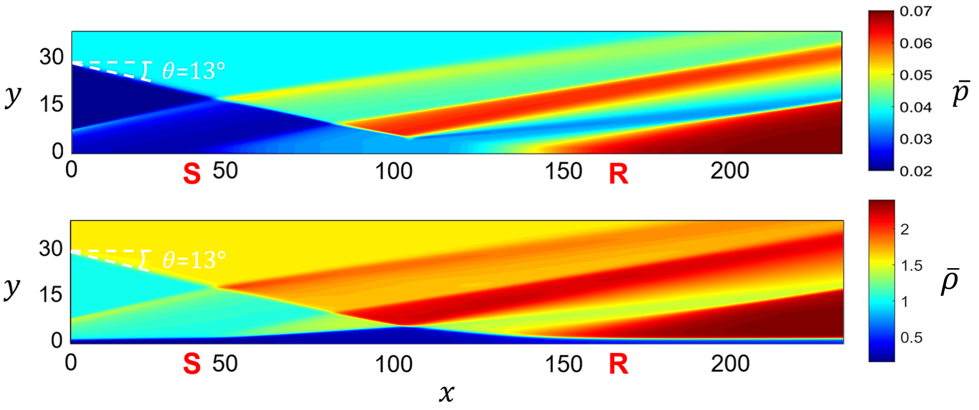
Figure 2: Contours of non-dimensional pressure and density for a 2D oblique shock wave/laminar boundary layer interaction with an incident shock angle of $\theta=13\degree$.

Figure 2(a) shows color contours of pressure while Figure 2(b) shows contours of density for SWBLI at $\theta=13\degree$. We non-dimensionalize $x$, $y$, and $z$ by the displacement thickness $\delta^{*}$. The incident oblique shock causes the boundary layer to separate from the wall at $x\approx 50$. At this location, we observe that a reflected shock forms. The separated boundary layer causes a recirculation bubble to form which has nearly constant density. At the apex of the recirculation bubble, an expansion fan forms and extends up into the freestream. At $x\approx 155$ the flow reattaches to the wall, and compression waves coalesce to form a second reflected shock. Figure 2(a) also shows a bow shock that enters the domain through the left inlet. This bow shock is created by the leading edge of the plate, and it does not interact with the recirculation bubble.

To visualize how the SWBLI changes with the incident shock angle, we plot streamlines and contours of streamwise velocity for several base flows in Figure 3. As the shock angle increases, the shock wave/boundary layer interaction becomes stronger, and the bubble size increases. Even though the oblique shock impingement point is the same in all of these simulations, the stronger recirculation in the cases with larger shock angles causes the boundary layer to separate from the wall earlier. The reattachment point shifts slightly downstream as the recirculation bubble becomes larger, but not as much as the separation point shifts upstream.

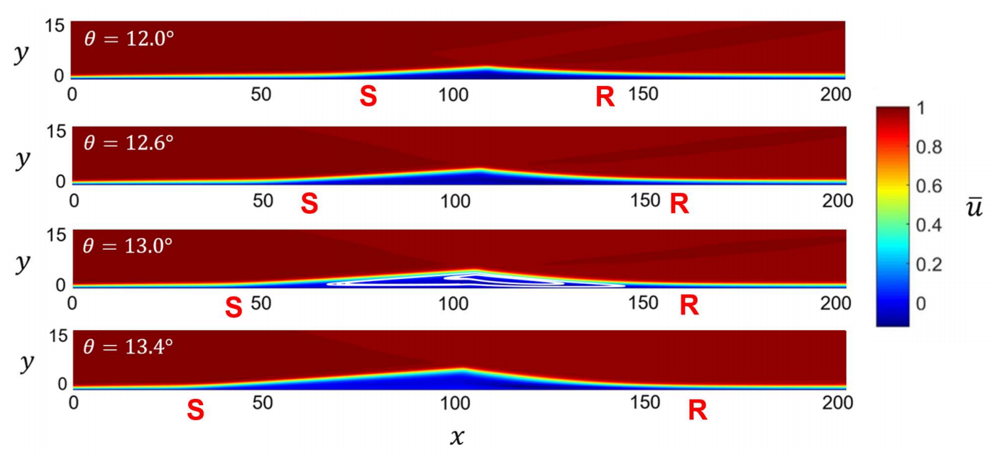
Figure 3: Contours of streamwise velocity for a 2D oblique shock wave/laminar boundary layer interaction with incident shock angles ranging from $\theta=12\degree$ (top) to $\theta=13.4\degree$ (bottom). For $\theta=13\degree$, white contours indicate streamlines inside the recirculation bubble. The separation and reattachment locations are indicated by “S” and “R,” respectively.

III.2 Direct numerical simulations

To study the dynamics of three-dimensional perturbations about the base flows, we perform three-dimensional DNS using the US3D hypersonic flow solver Candler . We initialize the 3D calculations by extruding the 2D base flow solutions in the spanwise direction. The spanwise length of our domain is 95.2$\delta^{*}$ with 200 uniformly distributed grid points. At the spanwise edges of the domain, we apply periodic boundary conditions. We do not apply any initial stochastic forcing to the flow field, and we find that the SWBLI remains 2D for an incident shock angle of $\theta=12.6\degree$ after integrating for more than 80 flow-through times.

Next, we repeat the DNS at an incident shock angle of $\theta=13\degree$. Unlike the previous case, the SWBLI starts to become three-dimensional after 15 flow-through times. Integrating further in time, we observe the flow to converge to a steady, three-dimensional solution after 80 flow-through times. Figure 4 shows the three-dimensional structure of this solution. In the figure, we plot color contours of spanwise velocity on an $xz$-plane close to the wall, as well as on three $yz$-planes at different streamwise positions. Grayscale contours of the density gradient magnitude on an $xy$-plane on the left show the shock structure together with the edges of the recirculation bubble. The spanwise velocity (and thus the three-dimensional flow) is mostly confined inside of the recirculation bubble. Some spanwise velocity is imparted to the flow downstream of the bubble, however, and plays a role in the formation of streaks.

Figure 4: Color contours of spanwise velocity shown on a wall-parallel plane close to the wall and three wall-normal planes for a 3D oblique shock wave/boundary layer interaction with $\theta=13\degree$. Grayscale contours of the density gradient magnitude are shown on a streamwise slice on the left.

In figure 4, we observe that three wavelengths of the 3D perturbation fit within the spanwise extent of our computational domain. Downstream, a more complicated pattern emerges. To investigate the spanwise spectral content of the flow as it develops downstream, we apply Fast Fourier Transforms (FFT’s) on a wall-parallel plane taken from the converged solution. Specifically, we apply FFT’s in the spanwise direction to the streamwise velocity perturbation on the $xz$-plane at $y=1$. Figure 5 shows logarithmic color contours of the Power Spectral Density (PSD) of streamwise velocity as a function of the spanwise wavenumber $\beta$ and streamwise position $x$. We find much of the spectral energy to be concentrated around a dominant spanwise wavenumber of $\beta=0.25$. The nonlinear simulation also gives rise to several harmonics, which are strongest in the downstream portion of the recirculation bubble. Spanwise spectral content is largely absent outside of the recirculation bubble, although the PSD at $\beta=0.25$ shows a renewed growth as the flow approaches the right edge of the domain. In this rightmost region, streamwise streaks begin to form.

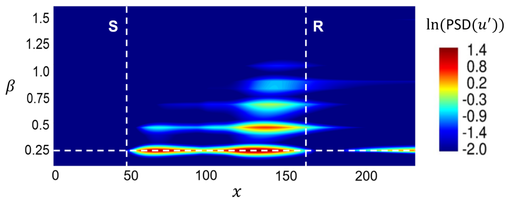
Figure 5: Streamwise variation of the spanwise PSD from the DNS with an incident shock angle of $\theta=13\degree$. Color contours on a logarithmic scale represent the PSD of the streamwise velocity perturbation as a function of streamwise position and spanwise wavenumber. The horizontal dashed line indicates the dominant spanwise wavenumber $\beta=0.25$. The recirculation bubble, bounded by the separation and reattachment locations (vertical dashed lines), contains most of the perturbation energy.

As the shock angle increases, more spanwise scales appear and the three-dimensional steady state eventually breaks down and the flow transitions to turbulence. At this point, the flow becomes unsteady and chaotic. Figure 6 shows incipient transition in SWBLI at a shock angle of $\theta=13.6\degree$. Similar to $\theta=13\degree$, the spanwise spectral content increases as the flow develops downstream, although in this case it ultimately leads to transition. While turbulent flow is chaotic and nonlinear, it is important to note that exactly three patches of transitioning flow are visible near the right edge of the domain. This matches the dominant spanwise wavenumber upstream, and agrees well with that found previously for $\theta=13\degree$. This suggests that the three-dimensional steady state found at lower shock angles still has a strong influence on the manner in which the flow transitions downstream of stronger shock wave/boundary layer interactions. Furthermore, in the following section, we show that global stability analysis can predict the bifurcation to this three-dimensional steady state, and that as such it may be understood in terms of linearized dynamics.

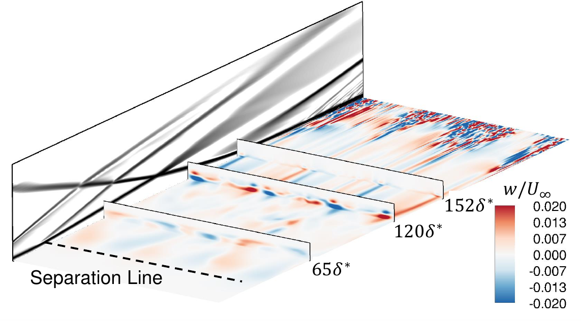
Figure 6: Color contours of spanwise velocity for SWBLI at $\theta=13.6\degree$. Contours are shown on the same planes as in figure 4, including grayscale contours of density gradient magnitude on the left.

III.3 Global mode analysis

To determine the critical incident shock angle at which the flow first becomes unstable, we apply global stability analysis over a range of shock angles and spanwise wavenumbers. For example, Figure 7 shows an eigenvalue spectrum resulting from the shift-and-invert Arnoldi method Lehoucq with a shock angle of $\theta=12.6\degree$ at a spanwise wavenumber $\beta=0.25$.

We express frequencies in non-dimensional form as Strouhal numbers defined as $St=f\delta^{*}/U_{\infty}$. The real and imaginary parts of the complex frequency $St=St_{r}+iSt_{i}$ denote the temporal frequency and growth rate, respectively. We position shifts along the real axis to capture the least stable modes, and twenty eigenvalues are converged at each shift. We space shifts close together so that a portion of the spectrum converged at each shift partially overlaps with a portion converged at neighboring shifts. Modes corresponding to redundant eigenvalues extracted by nearby shifts agree well with one another, providing one check on the convergence of the Arnoldi method. More eigenvalues can be found by using additional shifts or increasing the number of eigenvalues sought at each shift.

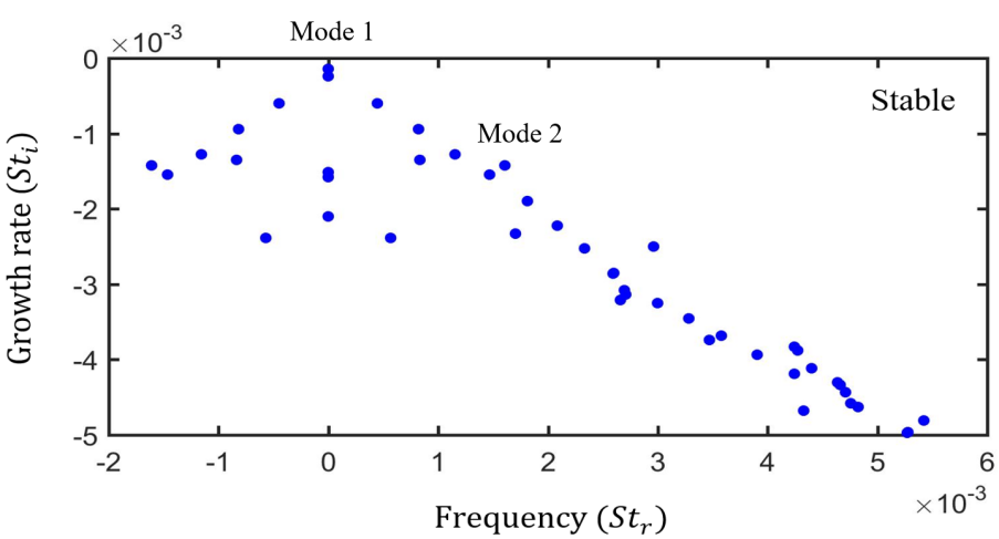
Figure 7: The eigenvalue spectrum of a SWBLI at $M_{\infty}=5.92$ from GSA with $\theta=12.6\degree$ and $\beta=0.25$.

Every eigenvalue in Figure 7 has a negative growth rate, which means the system is globally stable. This agrees with the DNS at $\theta=12.6\degree$ that remained 2D and steady. Figure 8 displays two eigenmodes and the position of three sponge layers. Mode 1 corresponds to the least stable, zero frequency eigenvalue. Notice that a significant portion of the perturbation lies within the recirculation bubble for this stationary global mode. We see a streamwise streak that extends downstream until it gets driven to zero by the right sponge layer. Mode 2, which corresponds to an oscillatory eigenvalue, has more structure within the recirculation bubble. In particular, the real part of the streamwise velocity perturbation in global mode 2 contains positive and negative components near the upstream portion of the bubble. This mode is structurally similar to the other surrounding oscillatory eigenmodes (not shown).

Figure 8: Stable global modes labeled in Figure 7 colored by the real part of the non-dimensional streamwise velocity perturbation. Here the dashed lines indicate the start of three different sponge layers.

Next, we increase the incident shock angle to $\theta=13\degree$ and repeat the same analysis, keeping the spanwise wavenumber fixed at $\beta=0.25$. Figure 9 shows the eigenvalue spectrum at these conditions. We see that one stationary eigenmode has a positive growth rate, which means the system is globally unstable. This agrees with the DNS at $\theta=13\degree$ that eventually produces a 3D steady state. Robinet found a similar unstable mode with zero frequency for an oblique shock wave/laminar boundary layer interaction at Mach 2.15 Robinet . Figure 10 displays the least stable, zero frequency eigenmode in 3D. This unstable global mode also contains long streamwise streaks similar to those shown in Figure 8 at a smaller incident shock angle. These elongated structures are clearly coupled to the shear layer on top of the recirculation bubble. We also see significant spanwise structure exists inside the recirculation bubble.

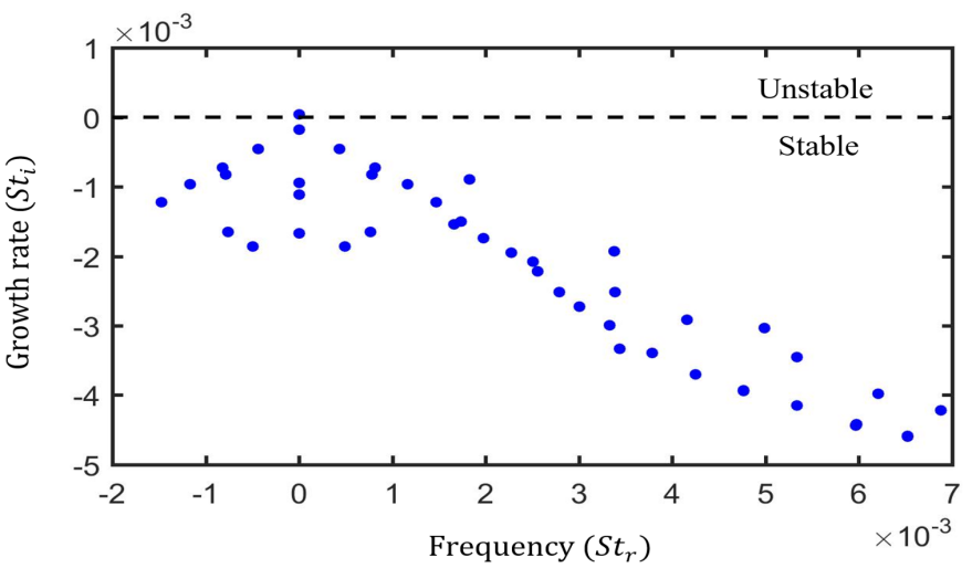
Figure 9: The eigenvalue spectrum of a SWBLI at $M_{\infty}=5.92$ from GSA with $\theta=13\degree$ and $\beta=0.25$. These conditions produce one eigenvalue in the unstable upper half plane. The unstable eigenvalue has zero frequency, indicating stationary instability.

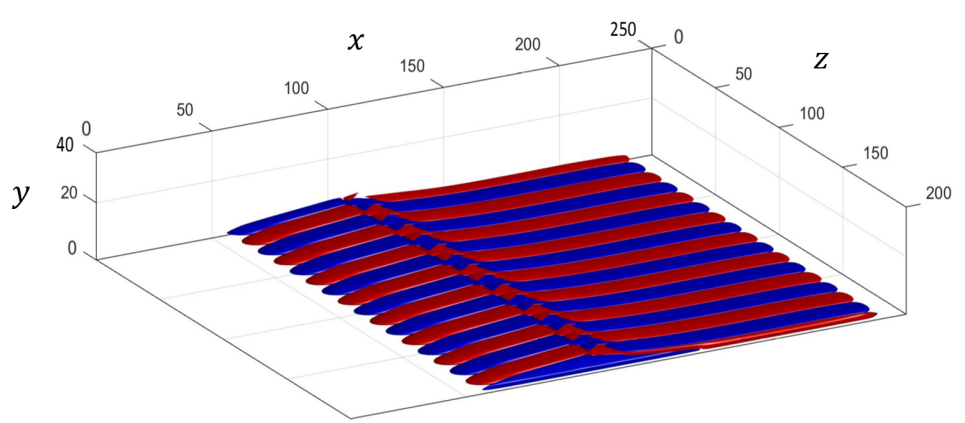
Figure 10: Isosurface contours of streamwise velocity perturbations induced by the least stable global mode for $\theta=13\degree$ and $\beta=0.25$. Red and blue contours indicate positive and negative velocity, respectively. This mode corresponds to the eigenvalue in the unstable half plane in Figure 9.

While $\theta=13\degree$ supports global instability over a range of spanwise wavenumbers, GSA of incident shock angles $\theta=12.6\degree$ and $\theta=12.8\degree$ revealed these cases to be globally stable at all spanwise wavenumbers. Increasing the shock angle to $\theta=12.9\degree$, however, resulted in instability at a single spanwise wavenumber $\beta=0.25$. Figure 11 shows the maximum growth rate versus spanwise wavenumber for angles ranging from $\theta=12.6\degree$ to $\theta=13\degree$. Above the critical incident shock angle $\theta=12.9\degree$, the 2D flow bifurcates to a 3D steady state with spanwise wavenumber $\beta=0.25$. The least stable global mode for every incident shock angle and spanwise wavenumber has zero frequency, meaning that such global modes are stationary at these conditions. In other words, the unstable global modes do not contain traveling waves or other oscillatory components, but instead simply grow exponentially while remaining in place, until they saturate and nonlinear effects become important. We see that $\beta=0.25$ results in the largest growth rate for every shock angle. These results agree with the DNS, and more specifically, Figure 5. As the spanwise wavenumber approaches zero, we expect the system to become fully stable because the base flows are 2D, and the 3D component of the perturbation gets smaller. The system stabilizes for non-dimensional spanwise wavenumbers above $\beta=0.4$.

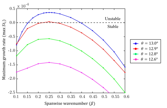
Figure 11: The maximum growth rate versus spanwise wavenumber for an oblique shock wave/laminar boundary layer interaction for four different incident shock angles.

While the GSA predicts the dominant spanwise wavenumber observed in DNS, we further verify that the unstable global mode (Figure 10) corresponds to the one observed in DNS (Figure 6), by introducing the mode obtained from GSA into the DNS and measuring its growth rate. For this purpose, we add the unstable global mode obtained for a shock angle of $\theta=13\degree$ and a spanwise wavenumber of $\beta=0.25$ (the most unstable mode) to a three-dimensional DNS initialized with the steady two-dimensional base flow. The global mode is scaled so that its amplitude is small compared to the base flow. Figure 12 shows the $L_{2}$-norm of the three-dimensional streamwise velocity perturbation associated with the global mode as it develops in time. After an initial adjustment, the DNS matches the growth predicted by GSA closely. The initial adjustment likely owes to slight differences in numerical methods. To obtain an accurate growth rate from the DNS after adding the unstable global mode, we remove all numerical dissipation. Due to almost no dissipation, the shocks adjust slightly compared to the scheme used to obtain the steady base flows. A very small amount of numerical dissipation is needed to suppress numerical instabilities that otherwise contaminate the steady base flows and prevent convergence at very long times (much longer than the time considered in Figure 12). This explains the initial transient in Figure 12, and highlights the sensitivity of hypersonic flows to numerical methods. After this initial adjustment, we recover the the growth rate predicted from GSA almost exactly. Furthermore, the mode shape (Figure 10) is almost exactly the same as the eigenfunction predicted by GSA, after it makes very slight adjustments to changes in the base flow. This comparison provides confidence that our GSA results are relevant to the physics of the DNS, and that our global modes are robust to slight changes in the base flow and numerical methods.

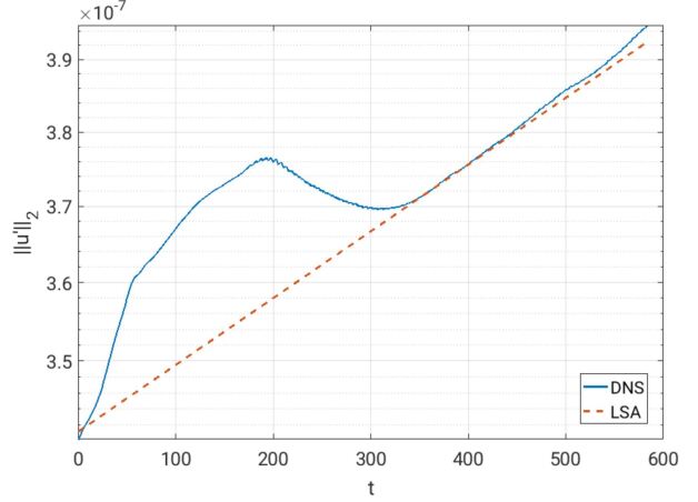
Figure 12: The temporal variation of the $L_{2}$-norm of an unstable stationary mode predicted by global stability analysis compared to the growth rate from the DNS after adding this global mode. This corresponds to an incident shock angle of $\theta=13\degree$ and a spanwise wavenumber of $\beta=0.25$.

IV DISCUSSION

As discussed in the previous section, GSA reveals that SWBLI becomes globally unstable at a critical shock angle of $\theta=12.9\degree$. Furthermore, at this shock angle, the analysis predicts the least stable global mode to be non-oscillatory and three-dimensional, with spanwise wavenumber $\beta=0.25$, in good agreement with DNS. While this provides useful information about the nature of the bifurcation, we now pursue a deeper understanding of the physical mechanism driving this instability. Determining a causal relationship between the different parts of a global mode can be challenging, because a global mode encompasses feedforward and feedback effects simultaneously. Nevertheless, by examining the shape of the critical global mode, we develop a fluid mechanical model of SWBLI instability in the first subsection below. In particular, we test the hypothesis that the feedforward part of the global mode relies upon centrifugal instability created by curved streamlines over the downstream portion of the recirculation bubble. Then, in the second subsection below, we mathematically investigate the origin of the critical global mode by applying an adjoint solver. Adjoint global modes show how SWBLI instability can be optimally triggered. Additionally, by overlapping direct and adjoint global modes, we find the spatial region where the instability is most sensitive to base flow modifications. All of these approaches work together to build a coherent picture of the physics responsible for SWBLI instability.

IV.1 Physical mechanism

Figures 13 and 14 show the effect of the least stable global mode with spanwise wavenumber $\beta=0.25$ at a shock angle of $\theta=13\degree$. As before, we select $\theta=13\degree$ to match the DNS results. To visualize the recirculation bubble, we add the global mode to the base flow, and compute the compressible streamfunction associated with the resulting flow in each $xy$-plane. The compressible streamfunction $\psi$ is defined such that $\rho\bm{u}=\bm{\nabla\times\psi}$ where $\bm{\psi}=[0\ 0\ \psi]$. The density inside the recirculation bubble is nearly constant (see Figure 2) so contours of $\psi$ closely approximate streamtraces computed by path integration of the velocity field. To compute $\psi$, we ignore the spanwise component of $\bm{u}$ because it is much smaller than the streamwise and wall-normal components. Also, since the global mode is stationary, the spanwise velocity perturbations are $90\degree$ out-of-phase relative to the streamwise and wall-normal perturbations. This means that in the $xy$-planes where the bubble reaches its maximum and minimum streamwise extents, the spanwise velocity perturbation is indeed exactly zero.

(a)	(b)

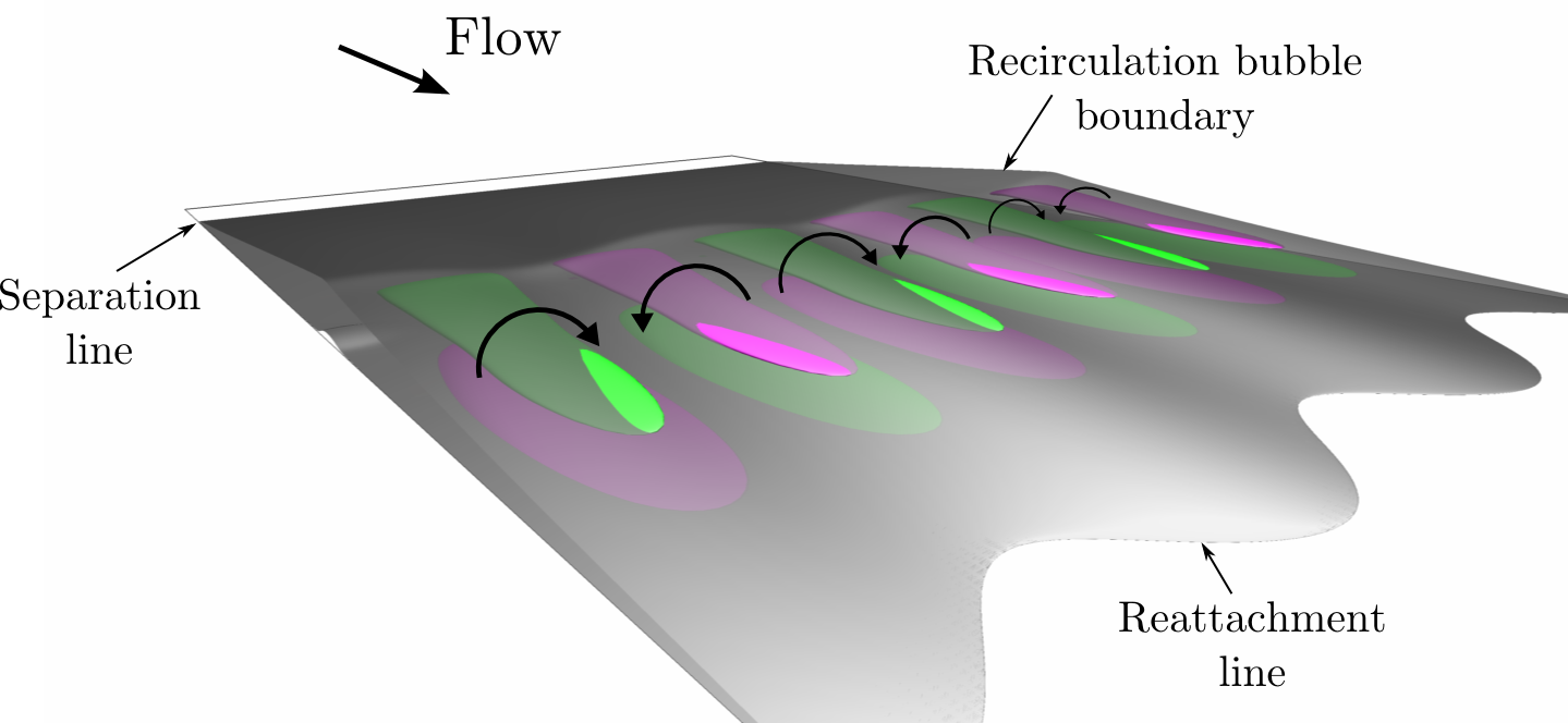
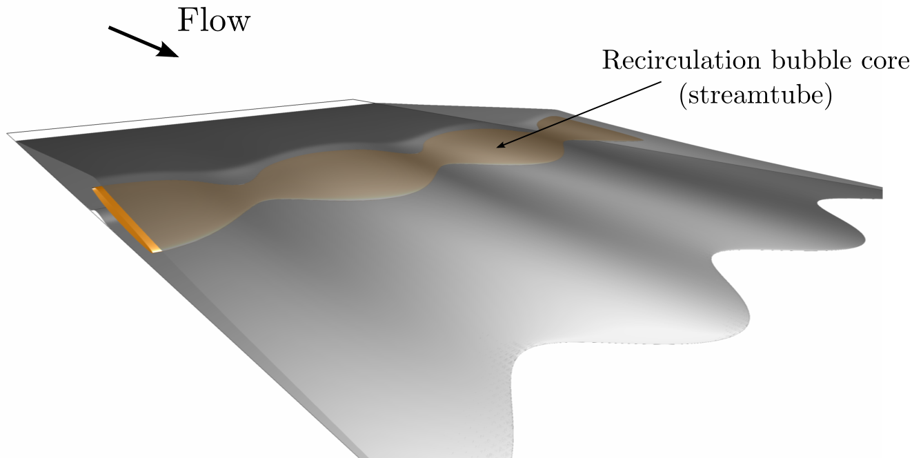
Figure 13: A rear view of the SWBLI recirculation bubble perturbed by the critical global mode. In both images, the gray separation streamsurface bounds the recirculating flow contained in the bubble. (a) Magenta and green isosurfaces of positive and negative streamwise vorticity show a spanwise array of counter-rotating streamwise vortices form just under the apex of the recirculation bubble. (b) The recirculation bubble expands and contracts periodically in span, in response to the streamwise vortices. The yellow surface represents another streamsurface, taken closer to the core of the recirculation bubble. See Supplemental Material at [URL will be inserted by publisher] for a movie showing these figures from different angles.

The gray isosurface shown in Figure 13(a) represents the separation streamsurface ($\psi=0$) which detaches from the wall along the separation line. Fluid underneath this surface stays inside the recirculation bubble whereas fluid outside this surface is deflected around the bubble. As such, this surface represents the boundary of the recirculation bubble.

Figure 13(a) also shows colored isosurfaces of streamwise vorticity inside the recirculation bubble. Because the base flow contains zero spanwise velocity and no spanwise gradients, any streamwise vorticity that develops is purely a consequence of perturbations owing to the three-dimensional global mode. As such, the shape of these patches of streamwise vorticity does not depend on the amplitude of the global mode relative to the base flow. These isosurfaces show that a spanwise periodic array of alternating streamwise vortices forms just below the apex of the bubble. Very close to the wall, patches of opposite vorticity form below these vortices, owing to shear created by the no-slip condition at the wall. The curved arrows in Figure 13(a) show the sense of the streamwise vortices just underneath the bubble apex. The counter-rotation of these vortices acts both to draw high-momentum fluid outside the bubble down close to the wall and to push low-momentum fluid inside the bubble upwards into the flow, in an alternating pattern along the spanwise direction. This causes both a spanwise undulation in the apex of the bubble, and a corresponding undulation in the reattachment line. Owing to the obliqueness of the angles in this hypersonic flow, the variation in the reattachment line location is much larger than the variation of the bubble height.

The spanwise variation of the reattachment line produces a corresponding spanwise modulation of the recirculation bubble strength as shown in Figure 13(b). Here, the yellow isosurface represents another surface of constant $\psi$, closer to the core of the spanwise vortex at the center of the recirculation bubble. In regions where the recirculation bubble is extended, the bubble core expands, and vice versa. Importantly, when the bubble core expands, it does so approximately equally in the upstream and downstream directions.

As the bubble expands, it pushes the base of the incident oblique shock slightly upstream. This forms a patch of positive pressure perturbation at the upstream end of the bubble core vortex as shown in Figure 14(a). At the same time, the expansion fan at the apex of the bubble grows and shifts slightly upstream, resulting in a negative pressure perturbation extending into the freestream. At spanwise locations corresponding to minimum bubble strength, this process occurs in reverse, resulting in corresponding pressure perturbations of opposite sign. Similar to the streamwise vortices found previously, the red and blue isosurfaces of positive and negative perturbation pressure (respectively) are determined by the critical global mode only, and so are not dependent on its amplitude relative to the base flow.

(a)	(b)

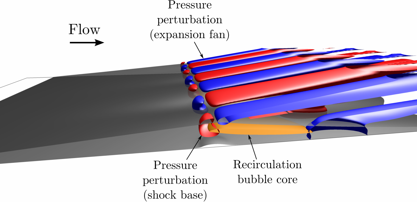
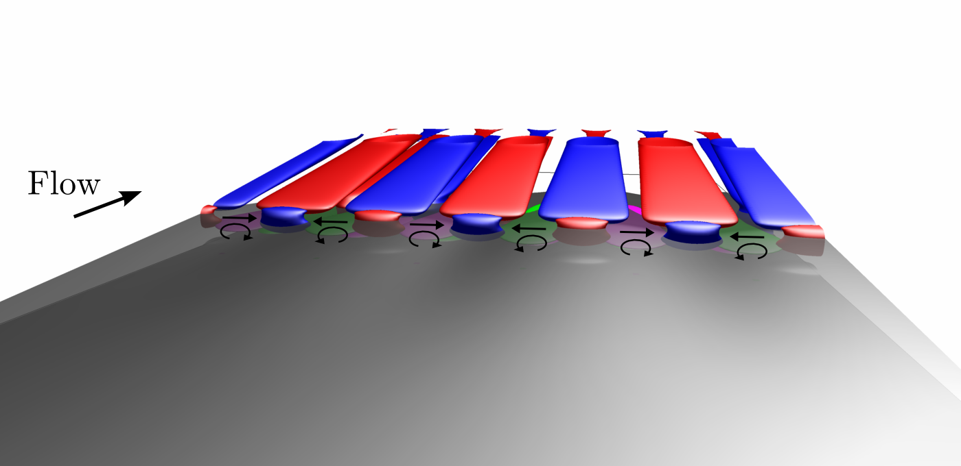
Figure 14: (a) A side view of the recirculation bubble (gray) perturbed by the same global mode shown in Figure 13. The front edge cuts through the spanwise location of maximum bubble strength (the spanwise position corresponding to the maximum streamwise extent of the bubble core as indicated by the yellow isosurface). At this spanwise location, the bubble pushes the impinging shock foot forward, producing a patch of positive pressure perturbation bounded by a red isosurface. Above the bubble, a shift in the expansion fan produces a negative pressure perturbation bounded by a blue isosurface. (b) The pressure perturbations produced by the impinging shock foot have the correct phase to drive the streamwise vortices (magenta and green isosurfaces) shown in Figure 13(a). See Supplemental Material at [URL will be inserted by publisher] for a movie showing these figures from different angles.

Finally, Figure 14(b) shows a front view of the pressure perturbations that develop at the base of the incident shock, relative to the streamwise vortices found previously. These pressure perturbations extend a short distance down into the recirculation bubble. When added to the base flow, these pressure perturbations would correspond to a spanwise corrugation of the incident shock base. From Figure 14(b), we see that the original spanwise vortices form just underneath these alternating pressure perturbations. The alternating pressure perturbations have the correct phase to provide a driving impulse to the streamwise vortices.

This completes the cycle that sustains the critical global mode. SWBLI instability forms from streamwise vortices created by corrugations at the base of the incident shock. These streamwise vortices modulate the recirculation bubble strength in a way that reinforces the incident shock corrugations. This stationary, three-dimensional instability is similar to a mechanism observed in laminar recirculation bubbles that form in incompressible fluid flow past backward-facing steps and bumps Barkley ; Gallaire ; Marquet08a . A similar mechanism is also active in laminar separation bubbles created by adverse pressure gradients applied to incompressible flat plate boundary layers, and provides an important route to three-dimensional flow independent of external excitation Rodriguez13 . For our high-speed flow, we visualize the three-dimensional nature of SWBLI instability by adding the global mode to the base flow and plotting streamlines as shown in Figure 15. We observe that the resulting streamlines follow surfaces of spanwise aligned torii sandwiched between locations of maximum and minimum recirculation bubble strength. In the upstream portion of the bubble, streamlines are driven away from the point marked $F(u)$ owing to the high pressure created by the corrugated shock base (see also Figure 14). In the downstream portion of the bubble, these streamlines do not recover completely in terms of their spanwise position. The net result is that fluid elements near the periphery of the recirculation bubble slowly move in the spanwise direction from regions of maximum bubble strength to regions of minimum bubble strength, over many recirculation cycles (indicated by the red streamlines). At the point of minimum bubble strength, fluid elements are attracted to a stable spiraling focus that forms in the bubble core. Still rotating, they are then rapidly injected back through the center of the torus to an unstable spiraling focus at the point of maximum bubble strength (blue streamlines). The outwards spiraling of streamlines at this unstable focus explains the equal magnitude upstream and downstream modulation of the bubble core shown in Figure 13(b). This toroidal motion of fluid elements inside the recirculation bubble is also consistent with the location of the patches of streamwise vorticity shown in Figure 13.

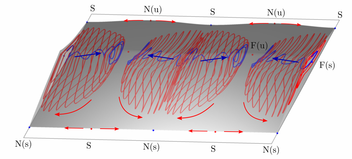
Figure 15: Toroidal streamline patterns inside the recirculation bubble created by three dimensional SWBLI instability. Corrugation of the impinging shock creates a region of high pressure just upstream of the point $F(u)$. This pushes streamline at the periphery of the recirculation bubble away from this point an towards the point $F(s)$. As they recirculate these streamlines (red) trace the exterior of a horizontally aligned torus. At $F(s)$, they are attracted to the center of the recirculation bubble and then quickly pass through the center of the torus to re-emerge close to $F(u)$.

Figure 16 summarizes how the global mode responsible for SWBLI instability modifies the flow topology. At the separation line, a series on no-slip critical points forms when the flow is perturbed three dimensionally. Because the flow along the wall is attracted to the separation line these critical points form an alternating sequence of stable nodes and saddle points. The reattachment line is similarly perturbed except an alternating sequence of unstable nodes and saddle points results. Different from low-speed separation bubbles Rodriguez10 , the stable nodes along the separation line and the unstable nodes along the reattachment line do not align in the streamwise direction. The result is that the flow along the wall is driven away from the regions of maximum bubble strength. Along the core of the bubble (dashed line) a sequence of stable and unstable spiraling foci then form to allow fluid elements to return to their original spanwise locations. While the amplitude of a global mode relative to the base flow is arbitrary (and continuously changing), the topological picture shown in Figure 16 is valid even for infinitesimal three dimensional perturbations, and so provides a valid description over a range of amplitudes. As the amplitude increases, the stable spiraling foci shift to lower positions, until they finally touch the wall. At this point, they each split into two no-slip stable spiraling foci, bounded upstream and downstream by two no-slip saddle points. Similar spiraling patterns have been observed in surface flow visualizations of SBLI experiments, although wind tunnel sidewall effects could not be ruled out as possible causes in such cases Bookey05 ; Dussauge05 ; Priebe09 .

Figure 16: Topology of three-dimensional SWBLI instability. No-slip critical points form along the separation and reattachment lines. Likewise, three-dimensional instability transforms the center associated with the core of two-dimensional recirculation bubble to a series of stable and unstable spiraling foci. While this pattern is reminiscent of three-dimensional instability in low-speed recirculation bubbles, the stable and unstable nodes along the separation and reattachment lines do not align for SWBLI. This creates the toroidal flow patterns shown in Figure 15.

The streamwise vortices responsible for the critical SWBLI global mode are not amplified by centrifugal instability. Figure 17 shows color contours of the Rayleigh discriminant,

$$\Delta=2\omega_{z}\frac{|\bar{\bm{u}}|}{R},$$ (7)

where $\omega_{z}$ is spanwise vorticity and $R$ is the local streamline curvature Sipp ; Gallaire ,

$$R=\frac{|\bar{\bm{u}}|^{3}}{\bm{\nabla}\psi\bm{\cdot}(\bar{\bm{u}}\bm{\cdot\nabla}\bar{\bm{u}})}.$$ (8)

Centrifugal instability can develop in regions where $\Delta<0$, which occurs when the vorticity and angular velocity of a fluid particle have opposite sign. Figure 17 shows that the Rayleigh discriminant does become negative for the SWBLI flow, but only outside of the recirculation bubble. In the figure, the separation streamline is represented by the white contour. The black lines, on the other hand, indicate contours of streamwise vorticity derived from the critical global mode. They reside inside the bubble, well away from regions of negative $\Delta$. In fact, the streamwise vortices form in a region of positive $\Delta$, where centrifugal effects are stabilizing. Therefore, while centrifugal instability (e.g., Görtler vortices) may play a role in amplifying disturbances outside and especially downstream of the recirculation bubble, we conclude that it plays no role in sustaining the critical global mode associated with SWBLI instability.

It is worth noting that in addition to Görtler instability, spatial transient growth due to the lift-up effect may also play a role in separation bubbles and lead to the formation and amplification of streamwise streaks Marxen ; Marquet2 . Quantification of this effect for SWBLI would be very interesting, but it would rely on non-modal stability analysis methodologies such adjoint-looping to identify optimal transient growth Dwivedi17 , which fall beyond the scope of this paper.

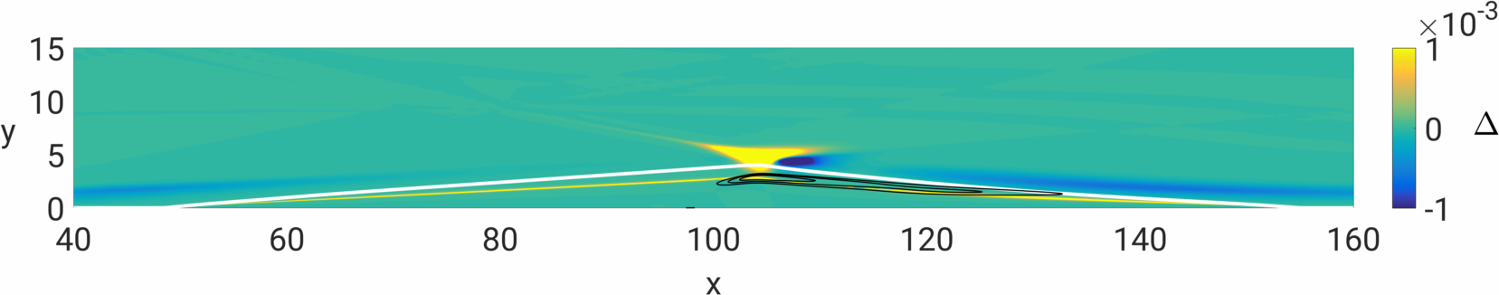
Figure 17: Color contours of the Rayleigh discriminant $\Delta$. Blue contours ($\Delta<0$) indicate regions that can support centrifugal instability, whereas yellow contours ($\Delta>0$) correspond to zones of stability with respect to centrifugal perturbations. The gray line represents the separation streamline. The black lines correspond to contours of streamwise vorticity from the critical global mode, showing the location of the streamwise vortices that support SWBLI instability.

IV.2 Adjoint analysis

While the fluid mechanics of SWBLI instability presented in the last subsection are compelling, we apply adjoint analysis to further understand the origin of this instability. While the direct linear system (4c) governs the behavior of effects of the instability, we derive an adjoint linear system that governs the sensitivity of the instability to its environment. In other words, analysis of this adjoint system uncovers what causes the instability to begin in the first place Chomaz .

For example, Figure 18 shows contours of adjoint streamwise velocity perturbation of the adjoint global mode corresponding to the direct mode shown in Figure 10. In the direct mode, the effects of SWBLI instability are evident inside the bubble and downstream. The corresponding adjoint mode, however, is active upstream, both in the incoming boundary layer and along the incident shock. This adjoint mode indicates where the critical global mode is most receptive to external perturbations, and so represents the optimal way to trigger the SWBLI instability. In fact, introducing small perturbations to the flow that align perfectly with the adjoint mode will, with the least amount of effort expended, cause the flow to respond via the direct global mode. Of course, external perturbations need not align exactly with this adjoint mode in order for the instability to activate. Rather, convolution of the adjoint mode with arbitrary disturbances (e.g., white noise) picks out those components that will initiate the instability, and so the adjoint mode can be thought of as a trigger for the instability.

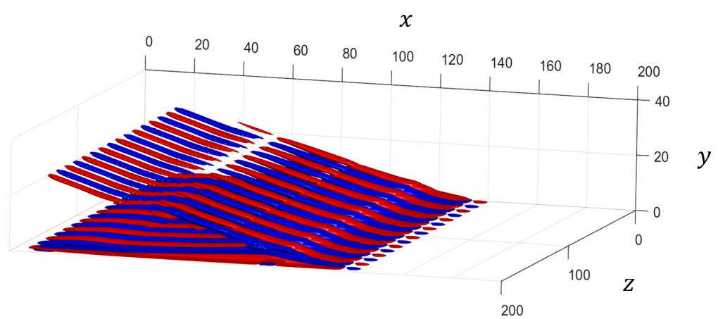
Figure 18: The adjoint mode corresponding to the critical direct global mode shown in Figure 10. Red and blue isosurface contours represent respectively positive and negative adjoint streamwise velocity perturbations.

The triggering mechanism provided by the adjoint global mode can be interpreted physically. For instance, the spanwise alternating pattern of velocity perturbations along the incident shock indicates that SWBLI instability can be initiated by the spanwise corrugation of the oblique shock. This agrees well with the fluid mechanical model presented above. Likewise, spanwise alternating fluctuations in the streamwise velocity of the incoming boundary layer can activate the instability through spanwise modulation of the bubble strength.

While the direct global mode in Figure 10 shows that the effects of SWBLI instability are felt mostly downstream, Figure 18 shows that the instability is precipitated from perturbations introduced mostly upstream. This spatial separation of the direct and adjoint global modes indicates significant non-normality of the Jacobian operator, caused by the strong convection present in the flow Schmid . Alteration of SWBLI instability therefore requires a balance between modifying sensitivity to upstream triggers and modifying the responsiveness of the system in terms of downstream effects. These modifications can be accomplished by changing the base flow slightly. In fact, one can show mathematically that an upper bound for the deviation of an eigenvalue $\partial\omega_{j}$ associated with the linear operator $A$ due to a structural perturbation $P$ (such as that created by changing the base flow slightly) is given by

$$|\partial\omega_{j}|\ \leq\ ||\bm{\hat{q}}_{j}||_{E}\ ||P||_{E}\ ||\bm{\hat{q}}_{j}^{+}||_{E},$$ (9)

where $\bm{\hat{q}}_{j}$ and $\bm{\hat{q}}_{j}^{+}$ are the direct and adjoint eigenmodes corresponding to the eigenvalue $\omega_{j}$, respectively Schmid ; Luchini ; Chomaz ; Marquet . Here, the subscript $E$ refers to an energy norm, such as those derived for compressible flow Hanifi . From (9), we can see that $P$ has the strongest effect when $||\bm{\hat{q}}_{j}||_{E}||\bm{\hat{q}}_{j}^{+}||_{E}$ is large. In physical terms, this is the region of space where the direct and adjoint global modes overlap Chomaz . For SWBLI, the overlap between direct and adjoint modes is greatest inside the bubble. The recirculation of the bubble provides the necessary balance between triggers and effects so that changing the base flow in this region modifies both processes, and can even result in stabilization of the system. Because the instability depends upon the details of the base flow where $||\bm{\hat{q}}_{j}||_{E}||\bm{\hat{q}}_{j}^{+}||_{E}$ is large, this region is called the “wavemaker” Chomaz . In essence, the wavemaker is the location where the base flow creates the instability.

Figure 19 shows color contours of $||\bm{\hat{q}}_{j}||_{E}||\bm{\hat{q}}_{j}^{+}||_{E}$ for the critical global mode for the shock angle $\theta=13\degree$. The white contour line represents the separation streamline, and the black contour lines are again three different levels of streamwise vorticity. The red color in Figure 19 indicates regions where SWBLI instability is most sensitive to base flow modification, i.e., the wavemaker. This figure shows that the wavemaker is contained almost exclusively inside the recirculation bubble. Furthermore, the region of maximum base flow sensitivity occurs just beneath the apex of the recirculation bubble. This is precisely the region where corrugations in the incident shock foot create streamwise vortices, according to the fluid mechanical model developed previously. This sensitive region also follows the streamwise vortices downstream. This suggests that these streamwise vortices form a crucial element of SWBLI instability, in good agreement with our fluid mechanical model.

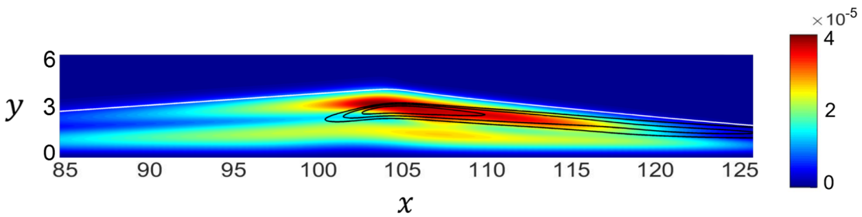
Figure 19: Color contours of $||\bm{\hat{q}}_{j}||_{E}||\bm{\hat{q}}_{j}^{+}||_{E}$ quantifying the overlap between the direct and adjoint critical global mode. Red corresponds to regions where SWBLI instability is most sensitive to base flow modification, or the “wavemaker.” The white line indicates the separation streamline, whereas the black lines represent contours of streamwise vorticity created by the critical global mode.

It is worth noting that the fact that the wavemaker is almost entirely contained within the recirculation bubble explains the insensitivity of the global mode to boundary conditions (sponge layers) at the edges of the computational domain. For SWBLI, the recirculation bubble and its interaction with the impinging shock foot completely determines the global mode dynamics, and are not affected by the sponge layers so long as the sponge layers are sufficiently far removed from the wavemaking region. This provides additional confidence in the physical relevance of the mechanism discussed above.

V CONCLUSIONS

We applied global stability analysis to find that an oblique shock wave impinging on a Mach 5.92 laminar boundary layer becomes linearly unstable for shock angles greater than $\theta=12.9\degree$ at the conditions studied. At the critical shock angle, the analysis predicted that a mode with spanwise wavenumber $\beta=0.25$ first becomes unstable, and that this mode does not oscillate in time. These predictions agreed well with results of three-dimensional direct numerical simulations.

The global stability analysis took into account strong streamwise gradients in the base flow such as that created by an impinging shock. It also allowed perturbations to propagate upstream as well as downstream, unlike methods based on the parabolized stability equations. Because of this, we were able to unravel the feedforward and feedback effects of the recirculation bubble to develop a physical model of the self-sustaining process responsible for SWBLI instability. We found that SWBLI instability depends crucially on the development of streamwise vortices within the recirculation bubble. These streamwise vortices redistribute streamwise momentum in the wall-normal direction and create a spanwise undulation in the reattachment line. The spanwise variation of the bubble length modulates its strength, creating corrugations in the oblique shock at its base, which in turn reinforce the original streamwise vortices.

Because the recirculation bubble creates significant streamline curvature in the flow, we investigated centrifugal instability as a possible mechanism for the creation of the streamwise vortices. We computed the Rayleigh discriminant for the flow and found that the streamwise vortices responsible for the instability form in a location where this quantity is positive so that the flow is stable with respect to centrifugal perturbations. We found that the Rayleigh discriminant does become negative, however, outside of the recirculation bubble so that centrifugal instability may play a role in the amplification of streaks downstream (see Dwivedi17 ). The streamwise vortices responsible for sustaining SWBLI instability, however, cannot be a consequence of centrifugal instability, but are created instead by spanwise corrugations at the base of the incident shock.

Adjoint analysis further confirmed the physical model of SWBLI instability as well as provided additional insight about the mechanisms responsible. The adjoint mode corresponding to the critical global mode indicated that SWBLI can be initiated by perturbations along the incident shock or in the upstream boundary layer. The former corresponds to corrugations in the incident shock, while the latter would result in spanwise periodic modulation of the recirculation bubble strength. Both of these effects were links in the self-sustaining cycle driving SWBLI instability, so this agreed well with our physical interpretation of the global stability results. Furthermore, by combining the critical direct and adjoint global modes, we calculated the sensitivity of SWBLI instability to modifications in the base flow. This analysis revealed that the spatial location of maximum sensitivity (the so-called wavemaker region) was almost entirely contained within the recirculation bubble. Furthermore, inside the bubble, the zone of peak sensitivity coincided with the streamwise vortices found previously. This once again indicated that SWBLI instability hinges upon the formation of streamwise vortices inside the recirculation bubble.

APPENDIX A: GLOBAL MODE SOLVER VERIFICATION

To verify our global mode solver, we run a few test cases that are presented in Malik . The base flow is locally parallel and consists of a boundary layer profile that satisfies the Mangler-Levy-Lees transformation. We model the bottom boundary as an adiabatic wall. Furthermore, we employ periodicity at the left and right boundaries of the domain. A sponge layer is placed along the top boundary, which we treat as a freestream outlet. Further, we use a stretched grid with $(n_{x},n_{y})=(101,301)$ and $y^{+}=0.6$ for every case. The Reynolds number ranges from 1000 to 3000, while the Mach number has a lower bound of 0.5 and goes up to 10. We consider stagnation temperatures between about 277.8 to 2333.3 K. There are no shocks present in this flow configuration.

Real and imaginary parts of the eigenvalue corresponding to the least stable global mode for each test case that we have computed with our global mode solver is compared against Malik’s results Malik . Table 1 displays these comparisons along with the case number. Note that only the second case has a non-zero spanwise wavenumber with $\beta=0.1$. The boundary layer displacement thickness changes for every case. We specify the streamwise wavenumber $\alpha$ for the first four test cases as 0.1, 0.06, 0.12, and 0.105, respectively. The last comparison is different in that we solve the spatial eigenvalue problem. For this we choose $\omega=0.23$, which is the angular frequency in Malik .

Table 1: A comparison of our global mode solver to Malik’s results Malik . Real and imaginary parts of the eigenvalue corresponding to the least stable global mode for five test cases are listed below. We define the length scale $\ell=\sqrt{\nu_{\infty}{x}/u_{\infty}}$, where $\nu_{\infty}$ is the kinematic viscosity in the freestream.

Case #	Malik’s #	$M_{\infty}$	$Re_{\ell}$	Real	Imaginary	Malik’s real	Malik’s imaginary
1	1	0.50	2000	0.0289	0.00223	0.0291	0.00224
2	3	2.50	3000	0.0362	0.00064	0.0367	0.00058
3	5	10.0	1000	0.1143	0.00017	0.1159	0.00015
4	4	10.0	2000	0.0982	0.00228	0.0975	0.00203
5	6	4.50	1500	0.2521	-0.00255	0.2534	-0.00249

We see from Table 1 that our global mode solver agrees well with previous stability calculations about high-speed boundary layers. For the first test case, we obtain almost exact agreement using the shift-and-invert Arnoldi method to obtain the least stable eigenmode. Notice at supersonic speeds we also get excellent agreement with Malik’s results Malik . As the Mach number increases to 10, our solutions start to deviate a small amount from the established values. Nevertheless, our global mode solver still predicts the established values to within 15% relative error in these extreme cases . Our formulation is different than some recent work on the stability of hypersonic boundary layers Balakumar because we utilize non-conservative state variables $p$, $\bm{u}$, and $s$ when solving for global modes. Our method is based on the characteristic formulation described in Sesterhenn and is similar to the method used in Mack2 to study instabilities in swept boundary layer flow at Mach 8.15. Table 1 shows that our method is able to accurately capture the relevant flow instability physics over a broad range of operating conditions of interest.

APPENDIX B: GRID INDEPENDENCE OF THE EIGENSPECTRA

Four grid resolutions are tested to study the convergence of our global mode solver. We use constant grid spacing in the streamwise direction for each resolution. Furthermore, the stretching function in the wall-normal direction does not change. The first grid has a total of 449,100 points, while the other three have approximately twenty, forty, and sixty percent less. We decrease the percentage of points in both the streamwise and wall-normal directions by the same amount. Here we focus our attention on the least stable modes.

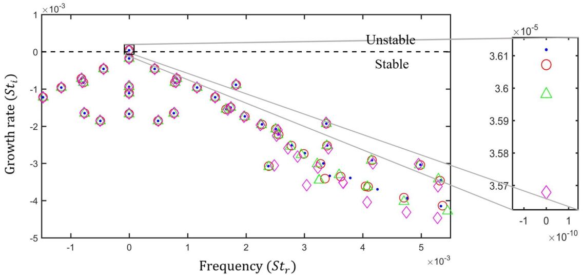
Figure 20: Eigenspectra that correspond to high (blue dots), medium (red circles), low (green triangles), and very low (magenta diamonds) resolution grids of the SWBLI for $\theta=13\degree$ and $\beta=0.25$. A closeup of the unstable eigenvalue is displayed on the right.

We consider an incident shock angle of $\theta=13\degree$ and a spanwise wavenumber of $\beta=0.25$. Figure 20 shows four eigenspectra pertaining to the various grid resolutions at this condition. We see most eigenvalues shift by only a small amount with increasing grid resolution. Eigenvalues at higher frequencies have a noticeable shift because they are part of the continuous spectrum. This is expected since there are fewer grid points in the freestream than there are close to the wall. To examine more precisely how the eigenvalues shift with grid resolution, the inset plot on the right hand side of Figure 20 shows a closeup view of the unstable eigenvalue. While the increment in resolution was constant between successive grids, we observe the eigenvalues shift significantly less between the two highest resolution grids. This indicates that the eigenspectrum is converged with respect to mesh resolution. While the axes of the inset figure are chosen to exaggerate the shift of the unstable eigenvalue, it is important to note that in fact it changes by less than 1.5% going from low to high resolution.

References

- (1) Frank M. White, Viscous Fluid Flow (McGraw-Hill, New York, 2006).
- (2) A. Pagella, U. Rist, and S. Wagner, Numerical investigations of small-amplitude disturbances in a boundary layer with impinging shock wave at Ma=4.8, Phys. Fluids 14, 2088 (2002).
- (3) R. Benay, B. Chanetz, B. Mangin, L. Vandomme, and J. Perraud, Shock wave/transitional boundary-layer interactions in hypersonic flow, AIAA J. 44, 1243 (2006).
- (4) J.-Ch. Robinet, Bifurcations in shock-wave/laminar-boundary-layer interaction: global instability approach, J. Fluid Mech. 579, 85 (2007).
- (5) F. Guiho, F. Alizard, and J.-Ch. Robinet, Instabilities in oblique shock wave/laminar boundary-layer interactions, J. Fluid Mech. 789, 1 (2016).
- (6) N. D. Sandham, E. Schülein, A. Wagner, S. Willems, and J. Steelant, Transitional shock-wave/boundary-layer interactions in hypersonic flow, J. Fluid Mech. 752, 349 (2014).
- (7) S. Gs, A. Dwivedi, G. V. Candler, and J. W. Nichols, Global linear stability analysis of high speed flows on compression ramps, AIAA Paper No. 2017-3455.
- (8) Ö. H. Ünalmis and D. S. Dolling, Decay of wall pressure field and structure of a Mach 5 adiabatic turbulent boundary layer, AIAA Paper No. 1994-2363.
- (9) B. Ganapathisubramani, N. T. Clemens, and D. S. Dolling, Effects of upstream boundary layer on the unsteadiness of shock-induced separation, J. Fluid Mech. 585, 369 (2007).
- (10) M. Wu and M. P. Martín, Direct numerical simulation of supersonic turbulent boundary layer over a compression ramp, AIAA J. 45, 879 (2007).
- (11) J. Délery and J. P. Dussauge, Some physical aspects of shock wave/boundary layer interactions, Shock Waves 19, 453 (2009).
- (12) E. Touber and N. D. Sandham, Large-eddy simulation of low-frequency unsteadiness in a turbulent shock-induced separation bubble, Theor. Comp. Fluid Dyn. 23, 79 (2009).
- (13) J. W. Nichols, J. Larsson, M. Bernardini, and S. Pirozzoli, Stability and modal analysis of shock/boundary layer interactions, Theor. Comp. Fluid Dyn. 30, 1 (2016).
- (14) S. Priebe and M. P. Martín, Low-frequency unsteadiness in shock wave-turbulent boundary layer interaction, J. Fluid Mech. 699, 1 (2012).
- (15) P. Dupont, J.-F. Debiève, J. P. Dussauge, J. P. Ardissonne, and C. Haddad, Unsteadiness in shock wave/boundary layer interaction, Aérodynamique des Tuyères et Arrières-Corps Working Group Report, 2003 (unpublished).
- (16) S. Piponniau, J. P. Dussauge, J.-F. Debiève, and P. Dupont, A simple model for low-frequency unsteadiness in shock-induced separation, J. Fluid Mech. 629, 87 (2009).
- (17) S. Pirozzoli and F. Grasso, Direct numerical simulation of impinging shock wave/turbulent boundary layer interaction at M=2.25, Phys. Fluids 18, 1 (2006).
- (18) A. Sansica, N. D. Sandham, and Z. Hu, Forced response of a laminar shock-induced separation bubble, Phys. Fluids 26, 1 (2014).
- (19) N. T. Clemens and V. Narayanaswamy, Low-frequency unsteadiness of shock wave/turbulent boundary layer interactions, Annu. Rev. Fluid Mech. 46, 469 (2014).
- (20) Z. R. Murphree, K. B. Yüceil, N. T. Clemens, and D. S. Dolling, Experimental Studies of Transitional Boundary Layer Shock Wave Interactions, AIAA Paper No. 2007-1139.
- (21) E. L. Lash, C. S. Combs, P. A. Kreth, and J. D. Schmisseur, Study of the Dynamics of Transitional Shock Wave-Boundary Layer Interactions using Optical Diagnostics, AIAA Paper No. 2017-3123.
- (22) L. M. Mack, Boundary-layer stability theory, Part B, Jet Propulsion Laboratory, Pasadena, California, Document No. 900-277, 1969.
- (23) A. Federov, Transition and stability of high-speed boundary layers, Annu. Rev. Fluid Mech. 43, 79 (2010).
- (24) G. V. Candler, P. K. Subbareddy, and I. Nompelis, in CFD Methods for Hypersonic Flows and Aerothermodynamics, edited by E. Josyula (AIAA, Virginia, 2015), pp. 203-237.
- (25) M. T. Semper, B. J. Pruski, and R. D. W. Bowersox, Freestream turbulence measurements in a continuously variable hypersonic wind tunnel, AIAA Paper No. 2012-0732.
- (26) J. Sesterhenn, A characteristic-type formulation of the Navier-Stokes equations for high order upwind schemes, Comput. Fluids 30, 37 (2001).
- (27) R. W. MacCormack, Numerical Computation of Compressible and Viscous Flow (AIAA Education Series, 2014).
- (28) J. W. Nichols and S. K. Lele, Global modes and transient response of a cold supersonic jet, J. Fluid Mech. 669, 225 (2011).
- (29) P. Shrestha, A. Dwivedi, N. Hildebrand, J. W. Nichols, M. R. Jovanović, and G. V. Candler, Interaction of an oblique shock with a transitional Mach 5.92 boundary layer, AIAA Paper No. 2016-3647.
- (30) P. K. Subbareddy and G. V. Candler, A fully discrete, kinetic energy consistent finite-volume scheme for compressible flows, J. Comput. Phys. 228, 1347 (2009).
- (31) F. Ducros, V. Ferrand, F. Nicoud, C. Weber, D. Darracq, C. Gacherieu, and T. Poinsot, Large-eddy simulation of the shock/turbulence interaction, J. Comput. Phys. 152, 517 (1999).
- (32) M. J. Wright, G. V. Candler, and M. Prampolini, Data-parallel lower-upper relaxation method for the Navier-Stokes equations, AIAA J. 34, 1371 (1996).
- (33) M. J. Wright, G. V. Candler, and D. Bose, Data-parallel line relaxation method for the Navier-Stokes equations, AIAA J. 36, 1603 (1998).
- (34) R. B. Lehoucq, D. C. Sorensen, and C. Yang, ARPACK Users’ Guide: Solution of Large-Scale Eigenvalue Problems with Implicitly Restarted Arnoldi Methods, (Society for Industrial and Applied Mathematics, 1998).
- (35) X. S. Li and J. W. Demmel, SuperLUDIST: A scalable distributed memory sparse direct solver for unsymmetric linear systems, ACM Trans. Math. Softw. 29, 110 (2003)
- (36) J. W. Nichols, S. K. Lele, and P. Moin, Global mode decomposition of supersonic jet noise, in Annual Research Briefs, Center for Turbulence Research, edited by P. Moin, N. N. Mansour, and S. Hahn (Stanford University, 2009), pp. 3-15.
- (37) A. Mani, On the reflectivity of sponge zones in compressible flow simulations, in Annual Research Briefs, Center for Turbulence Research, edited by P. Moin, J. Larsson, and N. N. Mansour (Stanford University, 2010), pp. 117-133.
- (38) D. Barkley, M. G. M. Gomes, and R. D. Henderson, Three-dimensional instability in flow over a backward-facing step, J. Fluid Mech. 473, (2002).
- (39) F. Gallaire, M. Marquillie, and U. Ehrenstein, Three-dimensional transverse instabilities in detached boundary layers, J. Fluid Mech. 571, 221 (2007).
- (40) O. Marquet, D. Sipp, J.-M. Chomaz, and L. Jacquin, Amplifier and resonator dynamics of a low-Reynolds-number recirculation bubble in a global framework, J. Fluid Mech. 605, (2008).
- (41) D. Rodríguez, E. M. Gennaro, and M. P. Juniper, The two classes of primary modal instability in laminar separation bubbles, J. Fluid Mech. 734, (2013).
- (42) D. Rodríguez and V. Theofilis, Structural changes of laminar separation bubbles induced by global linear instability, J. Fluid Mech. 655, 280 (2010).
- (43) P. B. Bookey, C. Wyckham, and A. J. Smits, Experimental investigations of Mach 3 shock-wave turbulent boundary layer interactions, AIAA Paper No. 2005-4899.
- (44) J.-P. Dussauge, R. Dupont, and J.-F. Debiève, Unsteadiness in shock wave boundary layer interactions with separation, Aero. Sci. Tech. 10(2), 85, (2005).
- (45) S. Priebe, M. Wu, and M. P. Martín, Direct numerical simulation of a reflected-shock-wave/turbulent-boundary-layer interaction, AIAA J. 47(5), 1173, (2009).
- (46) D. Sipp and L. Jacquin, Three-dimensional centrifugal-type instabilities of two-dimensional flows, Phys. Fluids 12, 7 (2000)
- (47) O. Marxen, M. Lang, U. Rist, O. Levin, and D. Henningson, Mechanisms for spatial steady three-dimensional disturbance growth in a non-parallel and separating boundary layer, J. Fluid Mech. 634, 165 (2009).
- (48) O. Marquet, M. Lombardi, J.-M. Chomaz, and D. Sipp, Direct and adjoint global modes of a recirculation bubble: lift-up and convective non-normalities, J. Fluid Mech. 622, 1 (2009).
- (49) A. Dwivedi, J. W. Nichols, M. R. Jovanović, G. V. Candler, Optimal spatial growth of streaks in oblique shock/boundary layer interaction, AIAA Paper No. 2017-4163.
- (50) J.-M. Chomaz, Global instabilities in spatially developing flows: non-normality and nonlinearity, Annu. Rev. Fluid Mech. 37, 357 (2005).
- (51) P. J. Schmid and D. S. Henningson, Stability and Transition in Shear Flows (Springer, New York, 2001).
- (52) P. Luchini and A. Bottaro, Adjoint equations in stability analysis, Annu. Rev. Fluid Mech. 46, 493 (2013).
- (53) O. Marquet, D. Sipp, and L. Jacquin, Sensitivity analysis and passive control of cylinder flow, J. Fluid Mech. 615, 221 (2008).
- (54) A. Hanifi, P. J. Schmid, and D. S. Henningson, Transient growth in compressible boundary layer flow, Phys. Fluids 8, 826 (1996).
- (55) M. R. Malik, Numerical methods for hypersonic boundary layer stability, J. Comput. Phys. 86, 376 (1990).
- (56) P. Balakumar, H. Zhao, and H. Atkins, Stability of hypersonic boundary-layers over a compression corner, AIAA J. 43, 760 (2005).
- (57) C. Mack, Ph.D. thesis, École Polytechnique, 2009.