Automatic Generation of Bounds for Polynomial Systems with Application to the Lorenz System

Abstract

This study covers an analytical approach to calculate positive invariant sets of dynamical systems. Using Lyapunov techniques and quantifier elimination methods, an automatic procedure for determining bounds in the state space as an enclosure of attractors is proposed. The available software tools permit an algorithmizable process, which normally requires a good insight into the systems dynamics and experience. As a result we get an estimation of the attractor, whose conservatism only results from the initial choice of the Lyapunov candidate function. The proposed approach is illustrated on the well-known Lorenz system.

1 Introduction

A dynamical system may have an attractor which implies a neighborhood around the attractor on which all trajectories are bounded. Thus, it is interesting to ask if such a neighborhood can be described analytically. From a geometric point of view, this means we intend to find a subset of the state space with some special properties, which is also called finding a compact invariant set or calculating an enclosure of the attractor. A standard procedure for calculating such a bound is to employ positive Lyapunov-like functions. However, there are two major restrictions to employing Lyapunov-like functions. A first is that the algebraic form as well as the parameterization of the function offers a considerable degree of choice, which usually makes finding a suitable candidate a matter of (mostly human) trail-and-error. A second is that calculating symbolic or numerical values of the bound on the Lyapunov-like candidate function that gives an estimate of the compact invariant set commonly requires human insight, experience, and frequently substantial algebraic manipulations. The approach we present here aims at circumventing these problems by proposing an automatic and algorithmizable procedure. This is done using quantifier elimination (QE) methods. The term quantifier elimination covers several methods [1, 2, 3] to reformulate quantified formulas into a quantifier free equivalent. This idea has already been applied for stability analysis [4, 5, 6, 7], model verification [8] as well as controller design [8, 9, 10].

The method we propose calculates an analytic expression of compact positive invariant sets. Moreover, if a dynamical system is dissipative and may consequently possess one (or even several) attractors, then a positive invariant set may contain at least one of them. However, attractors are invariant sets with additional requirements. They have to be compact, they are not dividable into two invariant, disjoint subsets and they need an attractive neighborhood. This consequently applies to chaotic attractors, which have a complicated geometry, and for which compact positive invariant sets can provide an enclosure. Thus, calculating attractor enclosures by compact positive invariant sets is related to, but differs in methodology and objective from computing analytic expressions of attractors themselves, as shown by calculating invariant measures and fractal dimension for the 2D Lorenz map [11, 12], or almost-invariant sets and invariant manifolds for the Lorenz system [13]. These differences in objective and methodology stem from this paper using Lyapunov–like function for calculating attractor enclosures, while calculating attractor approximations has been shown by either using a geometric description of the dynamics by invariant manifolds or a probabilistic description of dynamics by transfer operators or almost-invariants sets [14, 11, 15, 12, 13].

Although our method is generally applicable to dynamical systems with polynomial description, we specifically apply it to the Lorenz system to have a comparison with previous results. The Lorenz equations [16, 17] are arguable one of the best-known and most-studied dynamical systems that exhibit chaotic solutions. This also includes several works on ultimate bounds, compacts sets, or attractor enclosures [17, 18, 19, 20, 21, 22, 23, 24]. Apart from analyzing a property of the Lorenz system, calculating bounds is also a possible starting point for applications, for instance estimating the fractal dimension [25] or the Hausdorff dimension of the Lorenz attractor [24]. Attractor enclosures have additionally been used for the tracking of periodic solutions, stabilization of equilibrium points and synchronization [24, 26, 27].

The paper is structured as follows: In Section 2 we introduce our approach with briefly recalling quantifier elimination and calculating bounds on trajectories using Lyapunov-like functions. We also discuss how quantifier elimination can be used to obtain such bounds. The method is applied to the Lorenz system in Section 3. We calculate spherical and elliptical bounds with fixed and variable center points and show that our method can be used to reproduce, algebraically verify and partly improve bounds known from previous works [17, 20, 21]. In Section 4 we derive some conclusions.

2 Computation of Bounds for Dynamical Systems by Quantifier Elimination

2.1 Real Quantifier Elimination

Before we illustrate the proposed method let us briefly introduce some mathematical preliminaries on quantifier elimination (QE), cf. [28, 29], starting with a simple example to delineate the main ideas of QE.

Let us consider the quadratic function $g(x)=a_{2}x^{2}+a_{1}x+a_{0}$. The question if a parameter constellation $u=(a_{0},a_{1},a_{2})$ exists such that the function values $g(x)$ are always positive can be formulated using the quantified expression

$$\exists\,a_{2},a_{1},a_{0}~{}\forall x:g(x)>0,$$

which can easily be answered with true. If we are interested in all parameter constellations $u$, which result in $g(x)>0$, we utilize QE. Therefore, we omit the quantifiers for $u$ to generate an equivalent expression in these quantifier-free variables

$$\forall x:g(x)>0.$$

Applying a QE method to the problem we get

$$(a_{1}=0\lor 4a_{2}a_{0}-a_{1}^{2}\neq 0)\land a_{0}>0\land-4a_{2}a_{0}+a_{1}^{2}\leq 0.$$

Thus, we get exact conditions which are equivalent to the previous formula. After presenting the necessary fundamentals of QE, it is next shown how these techniques can be applied to estimate positive invariant sets.

In the following, we introduce the concept of quantifier elimination in a more formal way. An atomic formula is an expression of the form

$$\phi(x_{1},\ldots,x_{k})\;\tau\;0$$ (1)

with a relation $\tau\in\{>,=\}$, where $\phi\in\mathbb{Q}[x_{1},\ldots,x_{k}]$ is a polynomial in the variables $x_{1},\ldots,x_{k}$ with rational coefficients. A combination of atomic formulas (1) with the Boolean operators $\land,\lor,\lnot$ is called a quantifier-free formula. With these standard operators we can express all other Boolean operators such as equivalence ($\iff$) or implication ($\implies$) and augment the list of relations for (1) to $\{<,\leq,>,\geq,=,\neq\}$.

Let $F(u,v)$ be a quantifier-free formula in the variables $u=(u_{1},\ldots,u_{k})$ and $v=(v_{1},\ldots,v_{l})$. A prenex formula is an expression

$$G(u,v):=(Q_{1}v_{1})\cdots(Q_{l}v_{l})\,F(u,v)$$ (2)

with quantifiers $Q_{i}\in\{\exists,\forall\}$ for $i=1,\ldots,l$. The variables $v$ are called quantified and the variables $u$ are called free, respectively. Thus, the parameters $\{a_{2},a_{1},a_{0}\}$ gives the set $u$ and $\{x\}$ gives the set $v$ in the before described example of the quadratic equation. The quantifiers occurring in (2) can be eliminated [30, 31, 32]. This process is referred to as quantifier elimination. The following theorem is a direct consequence of the well-known Tarski-Seidenberg-Theorem [33, pp. 69-70]:

Theorem 1 (Quantifier Elimination over the Real Closed Field)

For every prenex formula $G(u,v)$ there exists an equivalent quantifier-free formula $H(u)$.

The first algorithm to determine such a quantifier-free equivalent was presented by Tarski itself. Unfortunately, this algorithm was not applicable because its computational complexity can not be bounded by any stack of exponentials. The first procedure which could be applied to non-trivial problems is cylindrical algebraic decomposition (CAD) [28]. This algorithm mainly consists of four steps. The first decompose the space in so-called cells in which every polynomial has a constant sign. Secondly, these cells are gradually projected from $\mathbb{R}^{n}$ to $\mathbb{R}^{1}$. These projections are cylindrical and algebraic. The conditions of interest are evaluated in $\mathbb{R}^{1}$ in the third step and the results are finally lifted to $\mathbb{R}^{n}$. Due to the universal applicability to the input sets of polynomials, this algorithm and its improvements (e.g. [34]) are still often used. Nevertheless, in the worst case the computational effort is doubly exponential in the number of variables [35].

The second commonly used procedure is virtual substitution [2, 36, 37]. The problem $\exists\,v:F(u,v)$ is solved with a formula substitution equivalent, where $a$ is substituted with terms of an elimination set. This procedure is just applicable to linear, quadratic and cubic polynomials, but the resulting complexity is ”just” exponential in the number of quantified variables. Furthermore, the resulting conditions are often very large and redundant such that a subsequent simplification is necessary.

A third frequently applied method for QE is based on real root classification (RRC). The number of real roots in a given interval can be computed using Sturm or Sturm-Habicht sequences. Based on that idea, formulations to eliminated quantifiers can be generated [38, 39, 40]. As in the case of virtual substitution the resulting output formulas are often very large and redundant such that a subsequent simplification is need as well. However, very effective algorithms can be achieved, especially for sign definite conditions $\forall v\geq 0\implies f(u,v)>0$, see [40].

To carry out the quantifier elimination we used the open-source software packages QEPCAD [34, 41], and REDLOG [42]. The later package is part of the computer algebra system REDUCE. For both tools, the resulting quantifier-free formulas can be simplified with the tool SLFQ [43]. The computations were carried out on a standard PC with Intel^® Core™ i3-4130 CPU at 3.4 GHz and 32 GiB RAM under the Linux system Fedora 25 (64 bit). For QE we used the advanced virtual substitution method from [44] (i.e., function rlqe with the switch on ofsfvs). The authors made the source code of prototype implementations publically available on Github [45] under the GNU GPL v3.0 in order to allow a verification of the presented results.

2.2 Bounds in Terms of a Lyapunov-like Function

Consider an autonomous nonlinear system

$$\dot{x}=f(x)$$ (3)

with the vector field $f:\mathcal{M}\to\mathbb{R}^{n}$ defined on an open subset $\mathcal{M}\subseteq\mathbb{R}^{n}$. We assume that (3) has a global solution $x(\cdot)$ for all $x(0)\in\mathcal{M}$. Bounds on system (3) are often formulated in terms of a continuously differentiable Lyapunov-like function $V:\mathcal{M}\to[0,\infty)$ and a constant $\gamma>0$ as

$$\limsup_{t\to\infty}V(x(t))\leq\gamma.$$ (4)

The computation of the bound $\gamma$ by (4) would require the knowledge of the solution $x(\cdot)$, which is generally not available for nonlinear systems. However, a bound $\gamma$ could be obtained using Lyapunov techniques by

$$\forall x\in\mathcal{M}:\quad V(x)>\gamma\;\implies\;\dot{V}(x)<0.$$ (5)

This means that the subset $\mathcal{E}:=\{x\in\mathcal{M}:\;V(x)\leq\gamma\}$ is positive invariant, i.e., for all initial values $x(0)\in\mathcal{E}$ we have $x(t)\in\mathcal{E}$ for all $t\geq 0$. Similarly, the bound $\gamma$ could be obtained from

$$\exists\alpha>0\;\forall x\in\mathcal{M}:\quad\dot{V}(x)\leq-\alpha\cdot(V(x)-\gamma),$$ (6)

where trajectories starting from $x(0)\notin\mathcal{E}$ converge to $\mathcal{E}$.

In general, the computation of $\gamma$ from (5) or (6) seems to be difficult since these formulas contain quantifiers. If $V$ and $\dot{V}$ are polynomials we could employ quantifier elimination in order to obtain a quantifier-free expression on the bound $\gamma$. As mentioned in Section 2.1, quantifier elimination is an algorithmizable process that removes the universal quantifier $\forall$ and the existential quantifier $\exists$ from the expressions (5) or (6). This process can be seen as a simplification as a quantifier-free formula for (5) or (6) may be obtained that can subsequently be evaluated automatically to get the bound $\gamma$. Within the restriction of computational feasibility, the procedure can even be extended to not only including the bound $\gamma$ but selected parameters of the candidate function $V$, for instance the center points of spherical invariant sets or the center points and axes of elliptical ones. Thus, the quantifier-free formula can be evaluated w.r.t. bounds and parameters of the Lyapunov-like function $V$.

3 Application to the Lorenz System

We apply our approach to the Lorenz system [16]

$$\begin{array}[]{lcl}\dot{x}_{1}&=&s(x_{2}-x_{1})\\ \dot{x}_{2}&=&r\,x_{1}-x_{2}-x_{1}x_{3}\\ \dot{x}_{3}&=&x_{1}x_{2}-bx_{3}\end{array}$$ (7)

with positive parameters $s,r,b>0$. In some cases we will use the parameter values

$$s=10,\quad r=28,\quad b=8/3.$$ (8)

3.1 Spherical Bounds with Fixed Center

First, we verify our approach using a well-known bound given in [20] based on the Lyapunov-like function

$$V_{1}(x)=x_{1}^{2}+x_{2}^{2}+(x_{3}-r-s)^{2}.$$ (9)

We consider level sets of (9) with $\gamma=c^{2}$ with $c>0$. Geometrically, these level sets are spheres with the radius $c$ around the fixed center point $(0,0,r+s)$. Defining

$$c_{1}:=\frac{(s+r)b}{2\sqrt{b-1}},\;c_{2}:=r+s,\;c_{3}:=\frac{(s+r)b}{2\sqrt{s(b-s)}}$$ (10)

the results presented in [20, Th. 2] can be stated as follows:

Theorem 2

A bound of (7) for $V_{1}(x)\leq c^{2}$ is given by

$$c=\left\{\begin{array}[]{lll}c_{1}&\text{for}&s\geq 1\land b\geq 2,\\ c_{2}&\text{for}&2s>b\land b<2,\\ c_{3}&\text{for}&2s\leq b\land s<1.\end{array}\right.$$ (11)

The associated partition of the parameter space $(s,b)$ is sketched in Fig. 1. The first case was already derived in [21] with $c=c_{1}=152/\sqrt{15}\approx 39.246$ for (8).

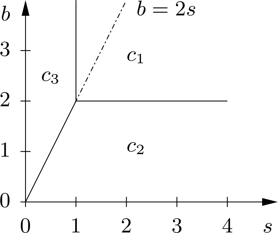
Figure 1: Parameter space for the bounds given in Th. 2

Using the Lyapunov-like function (9) we will derive bounds based on quantifier elimination. In our case, Eq. (5) has the form

$$\forall x_{1},x_{2},x_{3}:\quad s,r,b,c>0\land[V(x)>c^{2}\,\implies\,\dot{V}(x)<0]$$ (12)

with the quantified variables $x_{1},x_{2},x_{3}$. To obtain a quantifier-free representation of (12) w.r.t. the free variables $s,r,b,c$ we used the package REDLOG [42] with the computer algebra system REDUCE. We obtained expressions taking 4,3 KiB as plain ASCII code. Overall, the computation required approximately $250$ ms computation time on the above mentioned platform, where about $100$ ms where needed for quantifier elimination and about $150$ ms to execute the REDLOG script and to store the result. Simplifying these expressions with SLFQ [43] results after 130 QEBCAD calls in

$$c\geq r+1\;\land\;[ (b<2s\;\land\;b<2)\;\lor$$ (13a)

$$(\text{Ineq.~{}\eqref{eq:in1}}\;\land\;b<2s)\;\lor$$ (13b)

$$(\text{Ineq.~{}\eqref{eq:in2}}\;\land\;b<2)\;\lor$$ (13c)

$$(\text{Ineq.~{}\eqref{eq:in1}}\;\land\;\text{Ineq.~{}\eqref{eq:in2}})]$$ (13d)

with the inequalities

$$4(b-1)c^{2} \geq b^{2}(r+s)^{2},$$ (14)

$$4s(b-s)c^{2} \geq b^{2}(r+s)^{2}.$$ (15)

Clearly, the Ineqs. (14) and (15) correspond to the bounds $c_{1}$ and $c_{3}$ given in (10). Taking the different regions of the parameter space $(s,b)$ into account yields the bounds (11) given in Th. 2.

Remark 1

With our formal approach, we obtained the same bounds as in  [20, Th. 2] with just a slightly different formulation. Since (13) is equivalent to the quantified expression (12), the bounds given in Th. 2 are strict w.r.t. the levels sets of the Lyapunov function (9), i.e., with (9) the bounds (11) cannot be improved.

3.2 Spherical Bounds with Variable Center

Now, we consider levels sets of spheres around $(0,0,x_{30})$ with a variable displacement $x_{30}$ along the $x_{3}$-axis. This results in the Lyapunov-like function

$$V_{2}(x)=x_{1}^{2}+x_{2}^{2}+(x_{3}-x_{30})^{2}.$$ (16)

The quantifiers in the associated expression (5) could not be eliminated using REDUCE. Therefore, we turned our attention to (6) yielding

$$\exists\alpha\;\forall x_{1},x_{2},x_{3}:\quad\alpha,s,r,b,c>0\land\dot{V}(x)\leq-\alpha\cdot(V(x)-c^{2})$$ (17)

with the free parameters $\alpha,s,r,b,c,x_{30}$. The quantifier elimination with REDUCE using variable (e.g. unspecified) parameters results in 868 KiB ASCII text for the equivalent quantifier-free expression requiring a computation time of approximately $11.4$ s (including output and storage of the result). Unfortunately, we were not able to simplify these expressions with SLFQ. However, with fixed parameters (8) we obtained 37 KiB ASCII code in about $1.1$ s CPU time, which could be simplified with SFLQ after about 500 calls of QEPCAD (depending on the options) to

$$x_{30}^{2}-76x_{30}+1404<0\;\land\;(c\geq{c}_{4}\;\text{ with }\;a_{2}{c}_{4}^{4}+a_{1}{c}_{4}^{2}+a_{0}=0)$$ (18)

with the coefficients

$$\begin{array}[]{lcl}a_{0}&=&4096x_{30}^{4},\\ a_{1}&=&384x_{30}^{2}(3x_{30}^{2}-228x_{30}+4762),\\ a_{2}&=&9(x_{30}^{2}-76x_{30}+1404)(9x_{30}^{2}-684x_{30}+13436).\end{array}$$

The first inequality in (18) yields the open interval

$$31.676\approx 38-2\sqrt{10}<x_{30}<38+2\sqrt{10}\approx 44.524.$$ (19)

From the second term in (18) we can compute the bound $c_{4}$ on $c$ for a given point $x_{30}$ using the largest real root. The result is shown in Fig. 2. We have poles at the boundaries of the interval (19) since $a_{2}\to 0$ for $x_{30}\to 38\pm 2\sqrt{10}$.

Clearly, the choice $x_{30}=r+s=38$ from Section 3.1 with (8) is the center of the interval (19). However, the minimum of the bound $c$ occurs at a slightly different point as shown in Fig. 2. The solution of the biquadratic equation in (18) can be computed symbolically. The critical points are determined using the first derivative test. From (18) we compute the minimum $x_{30}\approx 36.118$ with $c_{4}\approx 38.1636$, which is an improvement compared to the radius computed in Section 3.1.

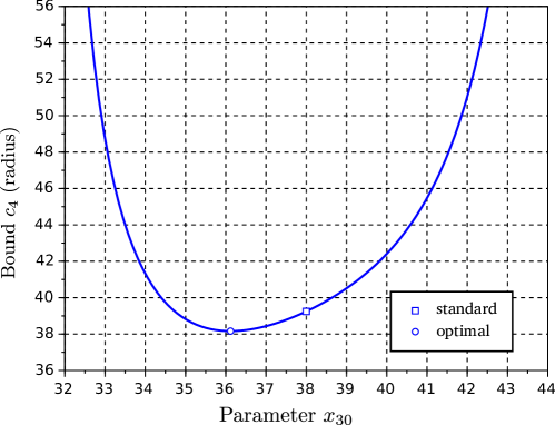
Figure 2: Bound $c_{4}$ depending on the parameter $x_{30}$

3.3 Elliptical Bounds with Fixed Axes and Fixed Center

Another well-known bound is derived in [17, Appendix C] using the Lyapunov-like function

$$V_{3}(x)=rx_{1}^{2}+sx_{2}^{2}+s(x_{3}-2r)^{2}.$$ (20)

The levels sets of (20) are ellipsoids around the center point $(0,0,2r)$ with a specific scaling of the axes. Quantifier elimination applying to the associated formula (5) directly yields

$$c^{2}\geq 4sr^{2}\;\land\;[ (b<2s\;\land\;b<2)\;\lor$$ (21a)

$$(\text{Ineq.~{}\eqref{eq:in3}}\;\land\;b<2s)\;\lor$$ (21b)

$$(\text{Ineq.~{}\eqref{eq:in4}}\;\land\;b<2)\;\lor$$ (21c)

$$(\text{Ineq.~{}\eqref{eq:in3}}\;\land\;\text{Ineq.~{}\eqref{eq:in4}})],$$ (21d)

with the inequalities

$$(b-1)c^{2} \geq sb^{2}r^{2},$$ (22)

$$(b-s)c^{2} \geq b^{2}r^{2}.$$ (23)

Taking the different regions of the parameters $b,s$ into account this leads immediately to the following theorem, which is similar to [17, Appendix C]:

Theorem 3

A bound of (7) for $V_{3}(x)\leq c^{2}$ is given by

$$c=\left\{\begin{array}[]{lll}br\sqrt{\frac{s}{b-1}}&\text{for}&s\geq 1\land b\geq 2,\\ 2r\sqrt{s}&\text{for}&2s>b\land b<2,\\ \frac{br}{\sqrt{b-s}}&\text{for}&2s\leq b\land s<1.\end{array}\right.$$ (24)

For the parameters (8) we obtain $c\approx 182.895$.

3.4 Elliptical Bounds with Fixed Axes and Variable Center

Similar as in Section 3.2 we replace the fixed center point of (20) by a variable one $(0,0,x_{30})$ and use the parameter set (8). This leads to the Lyapunov-like function

$$V_{4}(x)=rx_{1}^{2}+sx_{2}^{2}+s(x_{3}-x_{30})^{2}.$$ (25)

From the quantifier elimination with REDUCE we obtained 40 KiB ASCII source code in about $1.1$ s computation time, that could be reduced with SLFQ after about 500 QEPCAD calls to the quantifier-free formula

$$x_{30}>0\;\land\;(c\geq{c}_{5}\;\text{ with }\;a_{2}{c}_{5}^{4}+a_{1}{c}_{5}^{2}+a_{0}=0),$$ (26)

with the coefficients

$$\begin{array}[]{lcl}a_{0}&=&3211264x_{30}^{4},\\ a_{1}&=&10752x_{30}^{2}(3x_{30}^{2}-336x_{30}+10612),\\ a_{2}&=&9(x_{30}^{2}-112x_{30}+3024)(9x_{30}^{2}-1008x_{30}+29456).\end{array}$$

The biquadratic equation in (26) has only for

$$45.417\approx 56-4\sqrt{7}<x_{30}<56+4\sqrt{7}\approx 66.583$$ (27)

real roots. As in Section 3.2, the center of the interval is $x_{30}=2r=56$ as used in Section 3.3. Again, the minimum of $c$ occurs not at the center of (27) but at $x_{30}\approx 52.553$ with $c\approx 176.531$. The four bounds computed in Sections 3.1 to 3.4 are depicted in Fig. 3 as projections into the different two-dimensional planes.

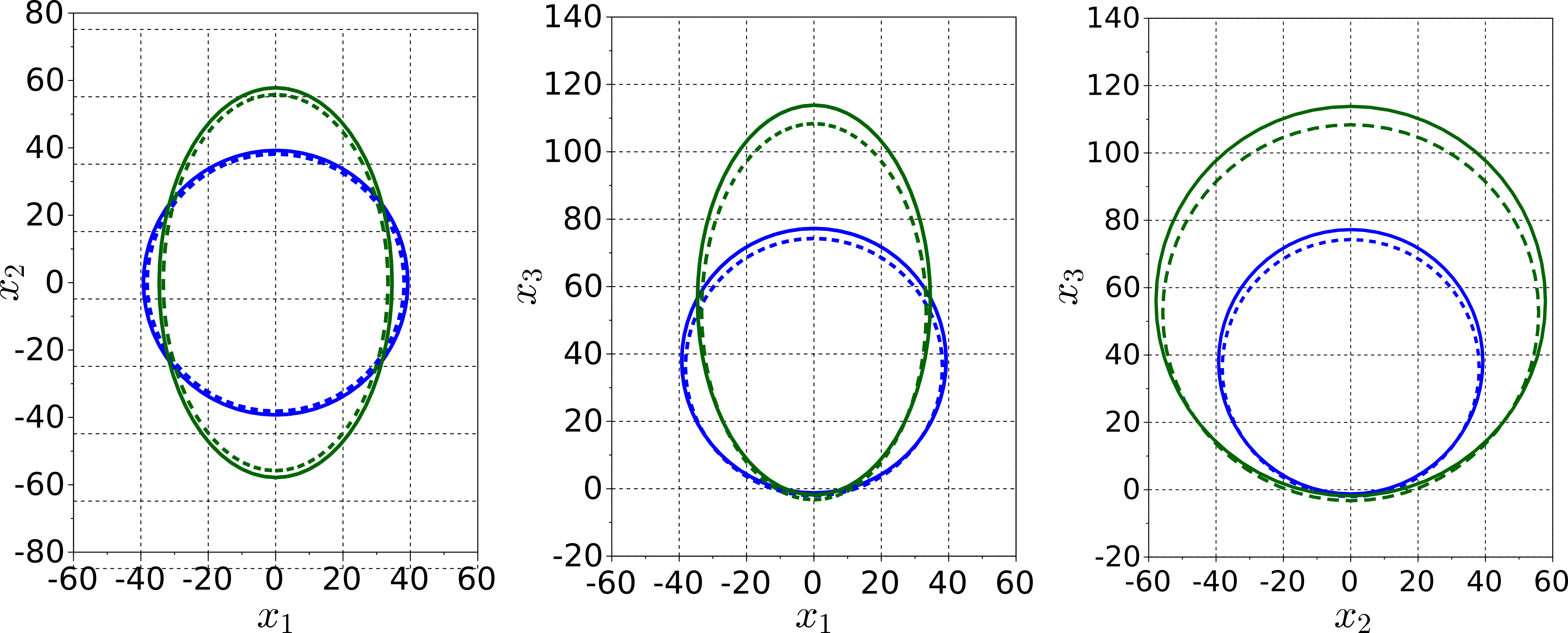
Figure 3: Projections of the bounds from Eq. (9) (blue, solid line), Eq. (16) (blue, dashed line), Eq. (20) (green, solid line), Eq. (25) (green, dashed line), respectively, into two-dimensional planes

3.5 Elliptical Bounds with Variable Axes and Center

The quadratic Lyapunov-like functions $V_{1},\ldots,V_{4}$ vary w.r.t. the scaling of the axes and the center point in the coordinate $x_{3}$. Generalizing these functions results in

$$V_{5}(x)=p_{1}x_{1}^{2}+p_{2}x_{2}^{2}+p_{3}(x_{3}-x_{30})^{2},$$ (28)

with $p_{1},p_{2},p_{3}>0$ and $x_{30}\in\mathbb{R}$. The large expression sizes discussed in Sections 3.2 and 3.4 suggest that we will not be able to solve the associated prenex formulas (5) or (6) with variable parameters. In addition to the system parameters (8) we used pre-determined parameters $p_{1},p_{2},p_{3},x_{30},c$ resulting in a prenex formula without free variables. Then, the equivalent quantifier-free formula (obtained after quantifier elimination) is either true or false.

For given parameters $p_{1},p_{2},p_{3},x_{30}$ we implemented a bisection method to approximately determine the boundary of $c$. We carried out a Monte Carlo simulation with uniformly distributed parameters $p_{1},p_{2},p_{3}\in[0.1,5]$ and $x_{30}\in[10,80]$. We did not find any admissible solution with $p_{2}\neq p_{3}$. This observation can be illustrated by the derivative

$$\begin{array}[]{rcl}\dot{V}_{5}&=&\;2(p_{3}-p_{2})x_{1}x_{2}x_{3}+(56p_{2}+20p_{1}-2p_{3}x_{30})x_{1}x_{2}\\ &&-\frac{16}{3}p_{3}x_{3}(x_{3}-x_{30})-20p_{1}x_{1}^{2}-2p_{2}x_{2}^{2}.\end{array}$$ (29)

The first term in (29) needs to be compensated to achieve negative definiteness for $\|x\|\gg 0$. This consideration leads to $p_{2}=p_{3}$ and restricts the set a suitable ellipsoids.

The ellipsoid given by $V_{5}(x)\leq c^{2}$ has the volume

$$\operatorname{vol}=\frac{4\pi}{3}\cdot\frac{c^{3}}{\sqrt{p_{1}p_{2}p_{3}}}.$$ (30)

Tab. 1 shows the bounds $c$ and the volumes of the associated ellipsoids for different parameters $p_{1},p_{2},p_{3},x_{30}$, where the Lyapunov-like functions $V_{1},\ldots,V_{4}$ are considered as special cases of $V_{5}$. For (28) we used $p_{1}=1$ and $p_{2}=p_{3}$. In order to minimize the volume of the positive invariant ellipsoid we carried out a Monte Carlo simulation. With this approach we were able to reduce the volume compared to the results given in Sections 3.1 to 3.4.

Table 1: Volumes of the ellipsoids for different parameter sets of function (28)

$V$	$p_{1}$	$p_{2}=p_{3}$	$x_{30}$	$c$	$\operatorname{vol}$
$V_{1}$	$1$	$1$	$38$	$39.246$	$2.532\cdot 10^{5}$
$V_{2}$	$1$	$1$	$36.1177$	$38.164$	$2.328\cdot 10^{5}$
$V_{3}$	$28$	$10$	$56$	$182.895$	$4.843\cdot 10^{5}$
$V_{4}$	$28$	$10$	$52.563$	$176.531$	$4.355\cdot 10^{5}$
$V_{5}$	$1$	$1.62$	$32.83$	$43.956$	$2.196\cdot 10^{5}$

After calculating several parameter constellations the union of the resulting ellipsoids gives a better approximation of the bounds then each individual one. This is shown in Figure 4. The union set can formally be described by the logical conjunction of the inequalities describing the ellipsoids.

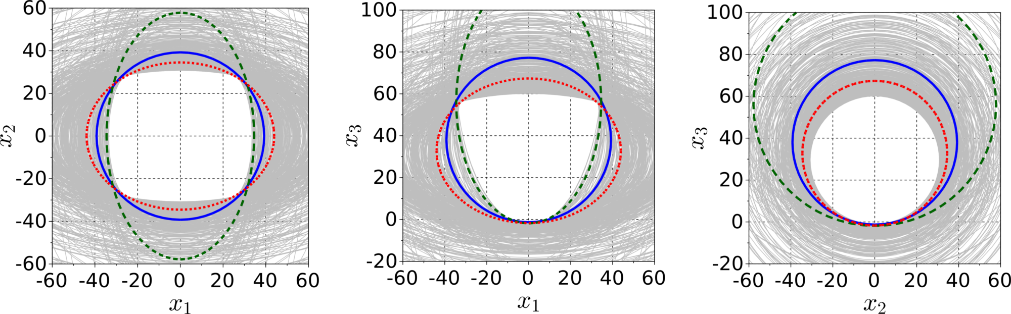
Figure 4: Bounds resulting from the union of 500 ellipsoids described by (28) (gray, thin lines), bound resulting from (9) with $c\approx 39.246$ (blue, bold solid line) and bound resulting from (20) with $c\approx 182.895$ (green, long dashes), best bound resulting from (28) by Monte Carlo simulation (red, short dashes)

4 Conclusions

The proposed approach gives a formal procedure to approximate the compact invariant set of nonlinear dynamical systems based on quantifier elimination methods. The resulting conservatism did not arise out of the calculation process itself but rather by the initial choice of the Lyapunov candidate. It was exemplarily shown how QE tools can be used to regenerate and improve known results in an automatic manner. The most challenging aspect are the inherent computational barriers of QE methods. To reduce the computational effort to a manageable scale, it is often necessary to preprocess or decompose the problem. Nevertheless, the proposed approach and quantifier elimination in general are very powerful and universal tools in system analysis and control.

In this paper we used quadratic Lyapunov-like functions with ellipsoids as level sets. With quadratic functions we could also describe cylinders or elliptic cones. Our approach is not restricted to quadratic Lyapunov-like functions, i.e., we could use high order polynomials. The Lorenz system discussed in the paper is a good example of a system with complicated dynamics having comparatively simple bounds. From our experience, complicated dynamics itself (such the existence of a chaotic attractor) may not necessarily be an obstacle for our approach. More important for a successful calculation is the relation between the systems dynamics and the geometry of the bound. In addition, higher order terms in the Lyapunov-like function can tighten the bound but may increase the computational effort significantly. Our method can be used to derive bounds for other nonlinear systems, e.g. for the Lorenz-Haken system.

References

References

- [1] G. E. Collins, Quantifier elimination for real closed fields by cylindrical algebraic decomposition–preliminary report, ACM SIGSAM Bulletin 8 (3) (1974) 80–90.
- [2] V. Weispfenning, The complexity of linear problems in fields, Journal of Symbolic Computation 5 (1-2) (1988) 3–27. doi:https://doi.org/10.1016/S0747-7171(88)80003-8.
- [3] B. F. Caviness, J. R. Johnson (Eds.), Quantifier Elimination and Cylindrical Algebraic Decomposition, Springer Science & Business Media, 2012.
- [4] H. Hong, R. Liska, S. Steinberg, Testing stability by quantifier elimination, Journal of Symbolic Computation 24 (2) (1997) 161–187. doi:http://dx.doi.org/10.1006/jsco.1997.0121.
- [5] T. V. Nguyen, Y. Mori, T. Mori, Y. Kuroe, QE approach to common Lyapunov function problem, Journal of Japan Society for Symbolic and Algebraic Computation 10 (1) (2003) 52–62.
- [6] Z. She, B. Xia, R. Xiao, Z. Zheng, A semi-algebraic approach for asymptotic stability analysis, Nonlinear Analysis: Hybrid Systems 3 (4) (2009) 588–596. doi:http://dx.doi.org/10.1016/j.nahs.2009.04.010.
- [7] R. Voßwinkel, K. Röbenack, N. Bajcinca, Input-to-state stability mapping for nonlinear control systems using quantifier elimination, in: European Control Conference (ECC), Limassol, Cyprus, 2018, accepted for publication.
- [8] T. Sturm, A. Tiwari, Verification and synthesis using real quantifier elimination, in: Proc. of the 36th International Symposium on Symbolic and Algebraic Computation, ACM, 2011, pp. 329–336.
- [9] M. Jirstrand, Nonlinear control system design by quantifier elimination, Journal of Symbolic Computation 24 (2) (1997) 137–152.
- [10] P. Dorato, Non-fragile controller design: an overview, in: Proc. American Control Conference (ACC), Vol. 5, Philadelphia, Pennsylvania, USA, 1998, pp. 2829–2831.
- [11] C. R. D. S. Graça, N. Zhong, Computing geometric Lorenz attractors with arbitrary precision, Trans. Amer. Math. Soc. 370 (4) (2018) 2955–2970. doi:https://doi.org/10.1090/tran/7228.
- [12] S. Galatolo, I. Nisoli, Rigorous computation of invariant measures and fractal dimension for maps with contracting fibers: 2D Lorenz-like maps, Ergodic Theory and Dynamical Systems 36 (6) (2016) 1865–1891. doi:doi:10.1017/etds.2014.145.
- [13] G. Froyland, K. Padberg, Almost-invariant sets and invariant manifolds – Connecting probabilistic and geometric descriptions of coherent structures in flows, Physica D: Nonlinear Phenomena 238 (16) (2009) 1507–1523. doi:https://doi.org/10.1016/j.physd.2009.03.002.
- [14] V. Araujo, S. Galatolo, M. J. Pacifico, Statistical properties of Lorenz-like flows, recent developments and perspectives, International Journal of Bifurcation and Chaos 24 (10) (2014) 1430028.
- [15] S. Galatolo, I. Nisoli, An elementary approach to rigorous approximation of invariant measures, SIAM Journal on Applied Dynamical Systems 13 (2) (2014) 958–985.
- [16] E. N. Lorenz, Deterministic non-periodic flow, J. Atmos. Sci. 20 (1963) 130–141.
- [17] C. Sparrow, The Lorenz Equations: Birfucations, Chaos, and Strange Atractors, Springer-Verlag, New York, 1982.
- [18] V. Reitmann, G. A. Leonov, Attraktoreingrenzung für nichtlineare Systeme, Vol. 97 of Teubner-Texte zur Mathematik, BSB Teubner, Leipzig, 1987.
- [19] A. P. Krishchenko, K. E. Starkov, Localization of compact invariant sets of the Lorenz system, Physics Letters A 353 (5) (2006) 383–388. doi:https://doi.org/10.1016/j.physleta.2005.12.104.
- [20] D. Li, J. an Lu, X. Wu, G. Chen, Estimating the bounds for the Lorenz family of chaotic systems, Chaos, Solitons & Fractals 23 (2) (2005) 529–534. doi:https://doi.org/10.1016/j.chaos.2004.05.021.
- [21] G. A. Leonov, A. I. Bunin, N. Koksch, Attractor localization of the Lorenz system, ZAMM - Journal of Applied Mathematics and Mechanics 67 (12) (1987) 649–656. doi:10.1002/zamm.19870671215.
- [22] M. Suzuki, N. Sakamoto, T. Yasukochi, A butterfly-shaped localization set for the Lorenz attractor, Phys. Lett. A 372 (15) (2008) 2614–2617.
- [23] F. Zhang, G. Zhang, Further results on ultimate bound on the trajectories of the Lorenz system, Qual. Theory Dyn. Syst. 15 (1) (2016) 221–235.
- [24] A. Y. Pogromsky, G. Santoboni, H. Nijmeijer, An ultimate bound on the trajectories of the Lorenz system and its applications, Nonlinearity 16 (5) (2003) 1597–1605.
- [25] V. A. Boichenko, G. A. Leonov, V. Reitmann, Dimension theory for ordinary differential equations, Teubner, Wiesbaden, 2005.
- [26] H. Richter, Controlling the Lorenz system: Combining global and local schemes, Chaos, Solitons & Fractals 12 (13) (2001) 2375–2380.
- [27] P. Yu, X. Liao, Globally attractive and positive invariant set of the Lorenz system, International Journal of Bifurcation and Chaos 16 (03) (2006) 757–764.
- [28] G. E. Collins, Quantifier elimination for real closed fields by cylindrical algebraic decompostion, in: Automata Theory and Formal Languages 2nd GI Conference Kaiserslautern, May 20–23, 1975, Springer, 1975, pp. 134–183.
- [29] B. F. Caviness, J. R. Johnson (Eds.), Quantifier Elimination and Cylindical Algebraic Decomposition, Springer, Wien, 1998.
- [30] A. Tarski, A Decision Method for a Elementary Algebra and Geometry, Project rand, Rand Corporation, 1948.
- [31] A. Tarski, A decision method for elementary algebra and geometry, in: Quantifier elimination and cylindrical algebraic decomposition, Springer, 1998, pp. 24–84.
- [32] A. Seidenberg, A new decision method for elementary algebra, Annals of Mathematics 60 (2) (1954) 365–374.
- [33] S. Basu, R. Pollack, M.-F. Roy, Algorithms in Real Algebraic Geometry, 2nd Edition, Springer, Berlin, Heidelberg, 2006.
- [34] G. E. Collins, H. Hong, Partial cylindrical algebraic decomposition for quantifier elimination, Journal of Symbolic Computation 12 (3) (1991) 299–328.
- [35] J. H. Davenport, J. Heintz, Real quantifier elimination is doubly exponential, Journal of Symbolic Computation 5 (1) (1988) 29–35. doi:https://doi.org/10.1016/S0747-7171(88)80004-X.
- [36] R. Loos, V. Weispfenning, Applying linear quantifier elimination, The Computer Journal 36 (5) (1993) 450–462.
- [37] V. Weispfenning, Quantifier elimination for real algebra — the cubic case, in: Proc. of the International Symposium on Symbolic and Algebraic Computation, ISSAC ’94, ACM, 1994, pp. 258–263.
- [38] L. Gonzalez-Vega, H. Lombardi, T. Recio, M.-F. Roy, Sturm-Habicht sequence, in: Proc. of the ACM-SIGSAM 1989 International Symposium on Symbolic and Algebraic Computation, ACM, 1989, pp. 136–146.
- [39] L. Yang, X. R. Hou, Z. B. Zeng, Complete discrimination system for polynomials, Science in China Series E Technological Sciences 39 (6) (1996).
- [40] H. Iwane, H. Yanami, H. Anai, K. Yokoyama, An effective implementation of symbolic–numeric cylindrical algebraic decomposition for quantifier elimination, Theoretical Computer Science 479 (2013) 43–69. doi:https://doi.org/10.1016/j.tcs.2012.10.020.
- [41] C. W. Brown, QEPCAD B: A program for computing with semi-algebraic sets using CADs, ACM SIGSAM Bulletin 37 (4) (2003) 97–108.
- [42] A. Dolzmann, T. Sturm, Redlog: Computer algebra meets computer logic, ACM SIGSAM Bulletin 31 (2) (1997) 2–9.
- [43] C. W. Brown, C. Gross, Efficient preprocessing methods for quantifier elimination, in: CASC, Vol. 4194 of Lecture Notes in Computer Science, Springer, 2006, pp. 89–100.
- [44] M. Košta, New concepts for real quantifier elimination by virtual substitution, Dissertation, Universität des Saarlandes, Fakultät für Mathematik und Informatik, Saarbrücken, Germany (2016).
-
[45]
Generation of bounds for the
Lorenz system using quantifier elimination. Source code of prototype
implementations.
URL https://github.com/TUD-RST/bounds-lorenz