A Primal-Dual Method for Optimal Control and Trajectory Generation in High-Dimensional Systems*

Abstract

Presented is a method for efficient computation of the Hamilton–Jacobi (HJ) equation for time-optimal control problems using the generalized Hopf formula. Typically, numerical methods to solve the HJ equation rely on a discrete grid of the solution space and exhibit exponential scaling with dimension. The generalized Hopf formula avoids the use of grids and numerical gradients by formulating an unconstrained convex optimization problem. The solution at each point is completely independent, and allows a massively parallel implementation if solutions at multiple points are desired. This work presents a primal-dual method for efficient numeric solution and presents how the resulting optimal trajectory can be generated directly from the solution of the Hopf formula, without further optimization. Examples presented have execution times on the order of milliseconds and experiments show computation scales approximately polynomial in dimension with very small high-order coefficients.

I Introduction

Hamilton–Jacobi equations play a fundamental role in optimal control theory as they establish sufficient conditions for optimality [1]. Traditionally, numerical solutions to HJ equations require a dense, discrete grid of the solution space [2, 3, 4]. Computing the elements of this grid scales poorly with dimension and has limited use for problems with dimension greater than four. The exponential dimensional scaling in optimization is sometimes referred to as the “curse of dimensionality” [5, 6]. Recent research [7, 8] has discovered numerical solutions based on the generalized Hopf formula that do not require a grid and can be used to efficiently compute solutions of a certain class of Hamilton–Jacobi PDEs that arise in linear control theory and differential games.

A key hurdle in the development of efficient high-dimensional solutions is the time-dependent Hamiltonian that results for general control problems. Kirchner et al. [8] applied the generalized Hopf formula with time-dependent Hamiltonian to efficiently solve multi-vehicle optimal pursuit-evasion using the linearized models found in [9]. In that work, the unique, specific structure of the model was used to derive a closed form solution to the gradient of the objection function, thereby allowing efficient optimization. This same technique cannot be applied to general linear systems and attempts to use numeric gradient approximation would increase computation time.

Darbon and Osher presented a proximal splitting algorithm in [7] using the split Bregman/ADMM approach [10], but this only applies to systems with time-independent Hamiltonians of the form $\dot{x}=f\left(u\left(t\right)\right)$, and has limited use for general linear control problems. Chow et al. [11] developed a coordinate descent method, but this optimization method lacks robustness for the nonsmooth optimization that typically result from the Hopf formula for optimal control problems.

This work presents a parallel proximal splitting optimization method [12] for solving time-optimal control problems with the generalized Hopf formula, including those with time-dependent Hamiltonians. This allows efficient solutions to generalized linear models, even when no explicit gradient of the objective function is known and without resorting to consensus-type algorithms [13]. Section II reviews using the Hopf formula for solutions to the Hamilton–Jacobi equations that arise in optimal linear control and largely follows the work of [8] and [7]. The main contributions of this paper are presented in Section III, with a primal-dual method for solving the Hopf formula, Section IV, which presents obtaining the optimal control, and Section V, where the optimal trajectory can be obtained directly from the solution of the Hopf formula. The new methods are applied on various time-optimal control problems and are presented in Section VI.

II Solutions to Hamilton–Jacobi Equations with the Hopf Formula

Consider system dynamics represented as

$$\dot{x}\left(t\right)=f\left(u\left(t\right)\right),$$ (1)

where $x\left(t\right)\in\mathbb{R}^{n}$ is the system state and $u\left(t\right)\in\mathcal{U}\subset\mathbb{R}^{m}$ is the control input, constrained to lie in the convex admissible control set $\mathcal{U}$. The system in $\left(\ref{eq: Basic diff eq}\right)$ describes how the state evolves in time and is considered a dynamic constraint when control inputs $u\left(t\right)$ are to be optimized. We consider a cost functional for a given initial time $t$, and terminal time $T$

$$K\left(x,u,t\right)=\int_{t}^{T}L\left(u\left(s\right)\right)ds+J\left(x\left(T\right)\right),$$ (2)

where $x\left(T\right)$ is the solution of $\left(\ref{eq: Basic diff eq}\right)$ at terminal time, $T$. We assume that the terminal cost function $J:\mathbb{R}^{n}\rightarrow\mathbb{R}$ is convex. The function $L:\mathbb{R}^{m}\rightarrow\mathbb{R}\cup\left\{+\infty\right\}$ is the running cost, and represents the rate that cost is accrued. The value function $v:\mathbb{R}^{n}\times(-\infty,T]\rightarrow\mathbb{R}$ is defined as the minimum cost, $K$, among all admissible controls for a given state $x$, and time $t\leq T$ with

$$v\left(x,t\right)=\underset{u\in\mathcal{U}}{\text{inf}}\,K\left(x,u,t\right).$$ (3)

The value function in $\left(\ref{eq: Value function}\right)$ satisfies the dynamic programming principle [14, 15] and also satisfies the following initial value Hamilton–Jacobi (HJ) equation by defining the function $\varphi:\mathbb{R}^{n}\times\mathbb{R}\rightarrow\mathbb{R}$ as $\varphi\left(x,t\right)=v\left(x,T-t\right)$, with $\varphi$ being the viscosity solution of

$$\begin{cases}\frac{\partial\varphi}{\partial t}\left(x,t\right)+H\left(\nabla_{x}\varphi\left(x,t\right)\right)=0&\text{in}\,\mathbb{R}^{n}\times\left(0,+\infty\right),\\ \varphi\left(x,0\right)=J\left(x\right)&\forall x\in\mathbb{R}^{n},\end{cases}$$ (4)

where the Hamiltonian $H:\mathbb{R}^{n}\rightarrow\mathbb{R}\cup\left\{+\infty\right\}$ is defined by

$$H\left(p\right)=\underset{c\in\mathbb{R}^{m}}{\text{sup}}\left\{\left\langle-f\left(c\right),p\right\rangle-L\left(c\right)\right\}.$$ (5)

We proceed with the Hamilton Jacobi formulation for time-optimal control to reach some convex terminal set $\Omega$, though the following methods can be generalized to other optimization problems. To apply the constraint that the control must be bounded, we introduce the following running cost $L=\mathcal{I}_{\mathcal{U}}$, where $\mathcal{I}_{\mathcal{C}}:\mathbb{R}^{n}\rightarrow\mathbb{R}\cup\left\{+\infty\right\}$ is the indicator function for the set $\mathcal{C}$ and is defined by

$$\mathcal{I}_{\mathcal{C}}\left(x\right)=\begin{cases}0&\text{if}\,x\in\mathcal{C}\\ +\infty&\text{otherwise.}\end{cases}$$

This reduces the Hamiltonian to

$$H\left(p\right)=\underset{c\in\mathcal{U}}{\text{max}}\left\langle-f\left(c\right),p\right\rangle.$$

Solving the HJ equation $\left(\ref{eq:Initial value HJ PDE}\right)$ describes how the value function evolves with time at any point in the state space, and from this optimal control policies can be found.

II-A Viscosity Solutions with the Hopf Formula

It was shown in [15] that an exact, point-wise viscosity solution to $\left(\ref{eq:Initial value HJ PDE}\right)$ can be found using the Hopf formula [16]. Moreover, no discrete grid is constructed, and the formula can provide a numerical method that is efficient even when the state space is high-dimensional. The value function can be found with the Hopf formula

$$\varphi\left(x,t\right)=-\underset{p\in\mathbb{R}^{n}}{\text{min}}\left\{J^{\star}\left(p\right)+tH\left(p\right)-\left\langle x,p\right\rangle\right\},$$ (6)

where the Fenchel–Legendre transform $g^{\star}:\mathbb{R}^{n}\rightarrow\mathbb{R}\cup\left\{+\infty\right\}$ of a convex, proper, lower semicontinuous function $g:\mathbb{R}^{n}\rightarrow\mathbb{R}\cup\left\{+\infty\right\}$ is defined by [17]

$$g^{\star}\left(p\right)=\underset{x\in\mathbb{R}^{n}}{\text{sup}}\left\{\left\langle p,x\right\rangle-g\left(x\right)\right\}.$$ (7)

II-B General Linear Models

Now consider the following linear state space model

$$\dot{x}\left(t\right)=Ax\left(t\right)+Bu\left(t\right),$$ (8)

with $A\in\mathbb{R}^{n\times n}$, $B\in\mathbb{R}^{n\times m}$, state vector $x\in\mathbb{R}^{n}$, and control input $u\in\mathbb{\mathcal{U}\subset R}^{m}$. We can make a change of variables

$$z\left(t\right)=e^{-tA}x\left(t\right),$$ (9)

which results in the following system

$$\dot{z}\left(t\right)=e^{-tA}Bu\left(t\right),$$ (10)

with terminal cost function now defined in $z$ with

$$\varphi\left(z,0\right)=J_{z}\left(z,0\right)=J_{x}\left(e^{TA}z\right).$$ (11)

For clarity in the sections to follow, we use the notation $H_{z}$ to refer to the Hamiltonian for systems defined by $\left(\ref{eq:z transformed system}\right)$, and $H_{x}$ for systems defined by $\left(\ref{eq:general linear system}\right)$. Additionally, with a slight abuse of notation, we denote by $J_{x}^{\star}\left(p,T\right)$ the Fenchel transform of $J\left(x,t\right)$ with respect to the variable $x$ at time $t=T$. Notice that the system $\left(\ref{eq:z transformed system}\right)$ is now time-varying, and it was shown in [18, Section 5.3.2, p. 215] that the Hopf formula can be generalized for a time-dependent Hamiltonian to solve for the value function of the system in $\left(\ref{eq:z transformed system}\right)$ with

$$\varphi\left(z_{0},T\right) =-\underset{p\in\mathbb{R}^{n}}{\text{min}}\Bigg{\{}J_{z}^{\star}\left(p,0\right)$$ (12)

$$+\int_{0}^{T}H_{z}\left(p,s\right)ds-\left\langle z_{0},p\right\rangle\Bigg{\}},$$

with $H_{z}$ defined as

$$H_{z}\left(p,t\right)=\underset{c\in\mathcal{U}}{\text{max}}\left\langle-e^{-\left(T-t\right)A}Bc,p\right\rangle.$$ (13)

The change of variable to $\left(T-t\right)$ is required for time since the problem was converted to an initial value formulation from a terminal value formulation in $\left(\ref{eq:Initial value HJ PDE}\right)$. The value function found by solving the unconstrained optimization problem in $\left(\ref{eq:generalized hopf formula}\right)$ can be thought of as the minimal cost of a system starting at initial state $z\left(0\right)=z_{0}$ and ending at terminal state $z\left(T\right)$.

Remark 1

While we are solving an initial value problem in this work, we can solve for a candidate solution of a two point boundary value problem (TPBVP) by selecting for the terminal set $\Omega$ a ball, and shrinking the radius until we get arbitrarily close to the terminal boundary condition of the corresponding TPBVP [19, Section 2.7.2, p. 66].

III Proximal Splitting Methods for Control

Proximal splitting methods [12] are a powerful group of convex optimization algorithms that efficiently solve non-smooth minimization problems in high dimensions. These methods are used for problems of the form

$$\underset{p\in\mathbb{R}^{n}}{\min}\,G\left(p\right)+F\left(p\right),$$

where proximal points for $G$ and $F$ can be easily computed. These family of methods have been proven effective for image processing and compressed sensing applications [10]. The proximal point of $f$ at $p$ for some $\alpha>0$ is given by

$$\left(I+\alpha\partial f\right)^{-1}\left(p\right) =\text{arg\,}\underset{w\in\mathbb{R}^{n}}{\text{min}}\left\{\alpha f\left(w\right)+\frac{1}{2}\left\|w-p\right\|_{2}^{2}\right\}.$$

The primal-dual algorithm [20] is a proximal splitting algorithm that solves the minimization problem of the form

$$\underset{p\in\mathbb{R}^{n}}{\min}\,G\left(p\right)+F\left(Kp\right),$$ (14)

with $K\in\mathbb{R}^{m\times n}$ and $G,F$ being assumed convex, by converting $\left(\ref{eq: primal CP}\right)$ to the saddle-point problem

$$\underset{p\in\mathbb{R}^{n}}{\min}\,\underset{y\in\mathbb{R}^{m}}{\max}\left\langle Kp,y\right\rangle+G\left(p\right)-F^{\star}\left(y\right).$$

The minimizer can be found by iterating the following update procedure

$$\begin{cases}y^{k+1}&=\left(I+\sigma\partial F^{\star}\right)^{-1}\left(y^{k}+\sigma K\bar{p}^{k}\right)\\ p^{k+1}&=\left(I+\tau\partial G\right)^{-1}\left(p^{k}-\tau K^{\top}y^{k+1}\right)\\ \bar{p}^{k+1}&=p^{k+1}+\theta\left(p^{k+1}-p^{k}\right),\end{cases}$$ (15)

until convergence with $\tau,\sigma>0$ being the primal and dual step sizes and $\theta\in\left[0,1\right]$. It was shown in [20] that the primal-dual method of $\left(\ref{eq: PD iterates}\right)$ converges at a rate of $\mathcal{O}\left(1/k\right)$ for general convex functions $F$ and $G$ provided the condition $\tau\sigma\left\|K\right\|^{2}<1$ is satisfied. If one or both of $F$ and $G$ are strongly convex, then [20] provides an alteration to the algorithm in $\left(\ref{eq: PD iterates}\right)$ that was shown to converge at a faster rate. While some problems in Section VI meet this criteria, these accelerated algorithms are outside the scope of this work, and all examples used the algorithm in $\left(\ref{eq: PD iterates}\right)$.

III-A Primal-Dual Solutions to the Generalized Hopf Formula

Suppose $\mathcal{U}$ is a closed convex set such that $0\in\text{int}\,\mathcal{U}$, where $\text{int}\,\mathcal{U}$ denotes the interior of the set $\mathcal{U}$. Then $\left(\mathcal{I}_{\mathcal{U}}\right)^{\star}$ defines a norm $\left\|\left(\cdot\right)\right\|$ and we denote by $\left\|\left(\cdot\right)\right\|_{*}$ its dual norm [17]. Also consider that the set $\mathcal{U}$ can be scaled by an injective linear transformation, $Q^{-1}$, to give the appropriate problem-specific control bound, then $\left(\ref{eq:Hamiltonian max form, linear}\right)$ can be written as

$$H_{z}\left(p,t\right)=\left\|\left(-e^{-\left(T-t\right)A}BQ\right)^{\top}p\right\|_{*}.$$ (16)

For simplicity, we follow [8] by approximating the integral in $\left(\ref{eq:generalized hopf formula}\right)$ with a left Riemann sum quadrature with $N$ equally spaced terms defined by

$$t_{i}=i\Delta t,$$ (17)

with $i\in\left\{0,\ldots,N-1\right\}$ and $\Delta t=\frac{T}{N}$. The generalized Hopf formula, for some terminal time $T$, becomes

$$\varphi\left(z_{0},T\right) =-\underset{p\in\mathbb{R}^{n}}{\text{min}}\Bigg{\{}J_{z}^{\star}\left(p,0\right)$$

$$+\Delta t\sum_{i=0}^{N-1}\left\|\left(-e^{-\left(T-t_{i}\right)A}BQ\right)^{\top}p\right\|_{*}$$

$$-\left\langle z_{0},p\right\rangle\Bigg{\}}.$$ (18)

Other forms of quadrature can be used for integral approximations, such as trapezoidal or Simpson’s rule [21], that increase approximation accuracy without sacrificing computational performance. Additionally, other advanced approximations could be considered, such as those employed by pseudospectral methods in [22], and will be investigated in future work.

To formulate as a primal-dual optimization, first set

$$G\left(p\right)=J_{z}^{\star}\left(p,0\right)-\left\langle z_{0},p\right\rangle.$$ (19)

Now define

$$K_{i}=\left(-e^{-\left(T-t_{i}\right)A}BQ\right)^{\top}$$ (20)

and $F_{i}=\Delta t\left\|\left(\cdot\right)\right\|_{*}=\left(\mathcal{I}_{\Delta t\mathcal{U}}\right)^{\star}$, where we denote by $\mathcal{I}_{\alpha\mathcal{C}}$ the indicator function of a set $\mathcal{C}$ scaled by a constant $\alpha>0$ defined as

$$\mathcal{I}_{\mathcal{\alpha C}}\left(x\right)=\begin{cases}0&\text{if}\,\frac{x}{\alpha}\in\mathcal{C}\\ +\infty&\text{otherwise.}\end{cases}$$

The sum term in $\left(\ref{eq: Generalized Hopf with quadrature}\right)$ can be written as

$$\Delta t\sum_{i=0}^{N-1}\left\|\left(-e^{-\left(T-t_{i}\right)A}BQ\right)^{\top}p\right\|_{*}=\sum_{i=0}^{N-1}F_{i}\left(K_{i}p\right).$$

We can now form the matrix $K$ as

$$K=\left[\begin{array}[]{c}K_{1}\\ K_{2}\\ \vdots\\ K_{N}\end{array}\right],$$

which gives

$$F\left(Kp\right)=\sum_{i=0}^{N-1}F_{i}\left(K_{i}p\right),$$ (21)

and combined with $\left(\ref{eq:G, for prox}\right)$ is now in the form of $\left(\ref{eq: primal CP}\right)$. Note that $K$ in this formulation is non square (preconditioning [23] can be used to enhance convergence rate). If the action of the matrix exponential in $\left(\ref{eq:K_i}\right)$ is not known, then it can be quickly evaluated, for all time samples, without resorting to computing the matrix exponential with [24]. The structure of $\left(\ref{eq: F as sum}\right)$ forms a separable sum. This implies that for some $y=\left(y_{1},y_{2},\ldots,y_{N}\right)$

$$F^{\star}\left(y_{1},y_{2},\ldots,y_{N}\right)=F_{1}^{\star}\left(y_{1}\right)+F_{2}^{\star}\left(y_{2}\right)+\cdots+F_{N}^{\star}\left(y_{N}\right).$$

Recall that $F_{i}=\left(\mathcal{I}_{\Delta t\mathcal{U}}\right)^{\star}$, thus

$$F_{i}^{\star}\left(y_{i}\right)=\mathcal{I}_{\Delta t\mathcal{U}}.$$ (22)

The proximal operator of a separable sum is simply

$$\left(I+\partial F^{\star}\right)^{-1}\left(y_{1},y_{2},\ldots,y_{N}\right)=\left[\begin{array}[]{c}\left(I+\partial F_{1}^{\star}\right)^{-1}\left(y_{1}\right)\\ \left(I+\partial F_{2}^{\star}\right)^{-1}\left(y_{2}\right)\\ \vdots\\ \left(I+\partial F_{N}^{\star}\right)^{-1}\left(y_{N}\right)\end{array}\right].$$ (23)

The proximal operators in $\left(\ref{eq:seperable prox}\right)$ are independent of each other, and as a result can be computed in parallel. This can be advantageous for real-time implementations in hardware such as multi-core embedded CPUs and field programmable gate arrays (FPGAs).

III-B Stopping Criteria

Care must be taken to select the stopping criterion of the algorithm in $\left(\ref{eq: PD iterates}\right)$. The step sizes $\tau$ and $\sigma$ are in general not equal and any stopping criteria must account for this. As a result we choose the primal and dual residuals [25, See Eqs. 10 and 12] as a step-size dependent stopping criteria and stop iterating $\left(\ref{eq: PD iterates}\right)$ when the conditions

$$\left\|\left(p^{k}-p^{k-1}\right)/\tau-K^{\top}\left(y^{k}-y^{k-1}\right)\right\|<\varepsilon,$$

and

$$\left\|\left(y^{k}-y^{k-1}\right)/\sigma-K\left(p^{k}-p^{k-1}\right)\right\|<\varepsilon,$$

are both met. For all the experiments listed in Section VI, $\epsilon$ is set to $10^{-4}$.

IV Time-Optimal Control

To find the time-optimal control to some convex terminal set $\Omega$, choose a convex terminal cost function $J_{x}$ such that

$$\begin{cases}J_{x}\left(x\right)<0&\text{for any}\,x\in\text{int}\,\Omega,\\ J_{x}\left(x\right)>0&\text{for any}\,x\in\left(\mathbb{R}^{n}\setminus\Omega\right),\\ J_{x}\left(x\right)=0&\text{for any}\,x\in\left(\Omega\setminus\text{int}\,\Omega\right),\end{cases}$$

where $\text{int}\,\Omega$ denotes the interior of $\Omega$. The intuition behind defining the terminal cost function this way is simple. If the value function $\varphi\left(x_{0},T\right)<0$ for some $x_{0}$ and $T$, then there exists a control $u\left(t\right)$ that drives the state from the initial condition at $x_{0}$ to the final state, $x\left(T\right)$, inside the set $\Omega$. The smallest value of time $T$, such that $\varphi\left(x_{0},T\right)=0$ is the minimum time to reach the set $\Omega$, starting at state $x_{0}$. Recall that the initial value function, $J_{z}\left(p,0\right)$, and its associated Fenchel–Legendre transform, $J_{z}^{\star}\left(p,0\right)$ of the Hopf formula in $\left(\ref{eq:generalized hopf formula}\right)$, is defined in $z$, and must be transformed with $\left(\ref{eq:Terminal cost as function of z}\right)$. The minimum time to reach $\Omega$ is denoted by $T^{*},$ and the control computed at $T^{*}$ is the time-optimal control. As first noted in [26], Hopf formula is itself a Fenchel–Legendre transform. It follows from a well known property of the Fenchel–Legendre transform [27] that the unique minimizer of $\left(\ref{eq:generalized hopf formula}\right)$ is the gradient of the value function

$$\nabla_{z}\varphi\left(z_{0},T\right) =\text{arg}\,\underset{p\in\mathbb{R}^{n}}{\text{min}}\Bigg{\{}J_{z}^{\star}\left(p,0\right)$$ (24)

$$+\int_{0}^{T}H_{z}\left(p,s\right)ds-\left\langle z_{0},p\right\rangle\Bigg{\}},$$

provided the gradient exists. So when solving for the value function using $\left(\ref{eq:generalized hopf formula}\right)$, we automatically solve for the gradient. We will refer to the minimizer in $\left(\ref{eq:gradient as argmin}\right)$ as $p^{*}=\nabla_{z}\left(z_{0},T\right)$.

We propose solving for the minimum time to reach the set $\Omega$, $T^{*}$, by a hybrid method of the bisection method and Newton’s method. Newton’s method has been shown to have faster convergence (quadratic) than bisection, but is unstable when the gradient is small and motivates the use of a hybrid method. We can iterate time, $t_{n+1}$, with Newton’s as

$$t_{n+1}=t_{n}-\frac{\varphi\left(x_{0},t_{n}\right)}{\frac{\partial\varphi}{\partial t}\left(x_{0},t_{n}\right)}.$$ (25)

As noted in [7], $\frac{\partial\varphi}{\partial t}\left(x_{0},t\right)$ must satisfy the Hamilton–Jacobi equation $\left(\ref{eq:Initial value HJ PDE}\right)$. Therefore we have

$$\frac{\partial\varphi}{\partial t}\left(x_{0},t_{n}\right)=-H_{x}\left(\nabla_{x}\varphi\left(x_{0},t_{n}\right),x_{0}\right).$$

We also see from $\left(\ref{eq:change of varibles}\right)$ and applying the chain rule that

$$\nabla_{x}\varphi\left(z\left(t\right),T-t\right) =\nabla_{x}\varphi\left(e^{-tA}x\left(t\right),T-t\right)$$

$$=e^{-tA^{\top}}\nabla_{z}\left(z\left(t\right),T-t\right).$$

Therefore when $t=0$, then $z_{0}=x_{0}$, $\varphi\left(z_{0},T\right)=\varphi\left(x_{0},T\right)$, and

$$\nabla_{x}\left(x_{0},T\right)=\nabla_{z}\left(z_{0},T\right).$$

This implies that $\left(\ref{eq:basic newton update}\right)$ can be written as

$$t_{n+1}=t_{n}+\frac{\varphi\left(z_{0},t_{n}\right)}{H_{x}\left(\nabla_{z}\varphi\left(z_{0},t_{n}\right),z_{0}\right)}.$$ (26)

For the purpose of evaluating $\left(\ref{eq:basic newton update with hamiltonian}\right)$, there is no need to apply the change of variables as in $\left(\ref{eq:change of varibles}\right)$. Therefore we have

$$H_{x}\left(p^{*},z_{0}\right)=-z_{0}^{\top}A^{\top}p^{*}+\left\|-Q^{\top}B^{\top}p^{*}\right\|_{*}.$$

If it is known that a single zero exists on the interval $T^{*}\in\left[0,t_{max}\right]$ then we use the Newton update from $\left(\ref{eq:basic newton update with hamiltonian}\right)$ to find $t_{n+1}$. With the value function computed at each Newton iteration, we can keep track of the updated interval $T^{*}\in\left[t_{min},t_{max}\right]$, and use a bisection update if the Newton update of $t_{n+1}$ is out side this interval. Once the minimum time to reach the set $\Omega$, $T^{*}$, is found, the optimal control $u^{*}\left(t\right)$ can be found from the relation

$$\nabla_{p}H_{z}\left(\nabla_{z}\varphi\left(z_{0},T^{*}\right),T^{*}\right) =\nabla_{p}H_{z}\left(p^{*},T^{*}\right)$$

$$=e^{-\left(T^{*}-t\right)A}Bu^{*}\left(t\right).$$ (27)

V Trajectory Generation with the Generalized Hopf Formula

Using the solution of the Hopf formula, we illustrate a dynamic programming point of view [6, 15] of the associated Hamilton–Jacobi equation to compute the optimal trajectory. We denote by $\gamma_{z}\left(s\right)\in\mathbb{R}^{n}$, with $s\in\left(0,T\right)$, as the state trajectory with $\gamma_{z}\left(0\right)=z_{0}$. Recall the fact that the solution of short-time Hopf formula $\left(\ref{eq: Basic Hopf formula}\right)$ is itself a Fenchel transform [26]

$$\varphi\left(z,t\right)=\left(J^{\star}+tH\right)^{\star}\left(z\right).$$ (28)

Note that the minimizer of $J_{z}^{\star}\left(p\right)$ is the optimal terminal state $\gamma_{z}\left(T\right)$, and, if $J_{z}^{\star}$ is differentiable, then can be found with

$$\gamma_{z}\left(T\right)=\frac{\partial}{\partial p}J_{z}^{\star}\left(p^{*},0\right),$$ (29)

where $p^{*}$ is the solution to the Hopf formula in $\left(\ref{eq: Basic Hopf formula}\right)$. Now consider the case where $p^{*}$ is the solution to the generalized Hopf formula given in $\left(\ref{eq:generalized hopf formula}\right)$, and what follows is an analysis in the variable $z$. This implies that

$$\varphi\left(z_{0},T\right) =-\Bigg{\{}J_{z}^{\star}\left(p^{*},0\right)+\Delta t\sum_{i=0}^{N-1}H_{z}\left(p^{*},t_{i}\right)$$ (30)

$$-\left\langle z_{0},p^{*}\right\rangle\Bigg{\}},$$

where each of the quadrature time samples $t_{i}$ are equally spaced by $\Delta t$ seconds on the interval $\left[0,T\right]$ as defined by $\left(\ref{eq:Left riemann time samples}\right)$. Recall from Section II-B that we denote by $\varphi_{z}^{\star}\left(p,T\right)$ the Fenchel transform of $\varphi\left(z,t\right)$ with respect to the variable $z$ at time $t=T$. If we write the Hopf formula with initial convex data $J\left(z,T-\Delta t\right)=\varphi\left(z,T-\Delta t\right)$, then we can find the level set evolution only for a short time, $\Delta t$, starting at value $\varphi\left(z,T-\Delta t\right)$ with

$$\varphi\left(z_{0},T\right) =-\Bigg{\{}\varphi_{z}^{\star}\left(p^{*},T-\Delta t\right)$$

$$=+\Delta tH_{z}\left(p^{*},T-\Delta t\right)-\left\langle z_{0},p^{*}\right\rangle\Bigg{\}}.$$

Following $\left(\ref{eq:terminal points}\right)$, the optimal state, with respect to $z$ is

$$\gamma_{z}\left(\Delta t\right)=\frac{\partial}{\partial p}\varphi_{z}^{\star}\left(p^{*},T-\Delta t\right).$$ (31)

From $\left(\ref{eq:Hopf is Fenchel}\right)$ we conclude that

$$\varphi_{z}^{\star}\left(p^{*},T-\Delta t\right) =\left(J^{\star}+\Delta tH_{z}\right)_{p}^{\star\star}\left(z,T-\Delta t\right)$$

$$=J_{z}^{\star}\left(p^{*},T-2\Delta t\right)$$ (32)

$$+\Delta tH_{z}\left(p^{*},T-2\Delta t\right).$$

The last line in $\left(\ref{eq:recursion}\right)$ is due to the fact that if $f$ is convex, proper and lower semicontinuous, then $f^{\star\star}=f$. We form a recursive operation, repeating $\left(\ref{eq:recursion}\right)$ until we reach time zero and get

$$\varphi\left(z_{0},T\right) =-\Bigg{\{}\varphi_{z}^{\star}\left(p^{*},0\right)$$

$$+\Delta t\sum_{i=0}^{N-1}H_{z}\left(p^{*},t_{i}\right)-\left\langle z_{0},p^{*}\right\rangle\Bigg{\}},$$

which is equivalent to $\left(\ref{eq:value of generalized hopf formula}\right)$ since by definition $J\left(x,0\right)=\varphi\left(x,0\right)$. This suggests that the generalized Hopf formula with the integral in $\left(\ref{eq:generalized hopf formula}\right)$ approximated by quadrature is equivalent to the composition of many short-time Hopf formulas $\left(\ref{eq: Basic Hopf formula}\right)$ of length $\Delta t$. Also, the recursion can be applied to the optimal terminal point from $\left(\ref{eq: next to last optimal trajectory}\right)$ as

$$\gamma_{z}\left(\Delta t\right) =\frac{\partial}{\partial p}\varphi_{z}^{\star}\left(p^{*},T-\Delta t\right)$$

$$=\frac{\partial}{\partial p}\left\{J_{z}^{\star}\left(p^{*},0\right)+\Delta t\sum_{i=0}^{N-1}H_{z}\left(p^{*},t_{i}\right)\right\}.$$

This can equivalently used for the optimal trajectory at any time sample $t_{i}$ as

$$\gamma_{z}\left(t_{i}\right) =\frac{\partial}{\partial p}\left\{J_{z}^{\star}\left(p^{*},0\right)+\Delta t\sum_{k=0}^{i}H_{z}\left(p^{*},t_{k}\right)\right\}$$ (33)

$$=\frac{\partial}{\partial p}J_{z}^{\star}\left(p^{*},0\right)+\Delta t\sum_{k=0}^{i}\frac{\partial}{\partial p}H_{z}\left(p^{*},t_{k}\right).$$

If we are interested in the trajectory at each quadrature time sample, we don’t have to recompute the sum for each $t_{k}$, since we can incrementally build the trajectory point from $t_{k+1}$. Note that each point in $\left(\ref{eq:optimal trajectory at sample}\right)$ is in terms of the state variable $z$, and can be found for $x$ by applying inverse of the transform given in $\left(\ref{eq:change of varibles}\right)$. Non-rigorously we see that the time rate of change of the state trajectory in $\left(\ref{eq:optimal trajectory at sample}\right)$ is equal to the gradient with respect to $p$ of the Hamiltonian, which satisfies Pontryagin’s Maximum Principal [28], though it was derived using only the Hopf formula and basic principals of convex analysis.

VI Results

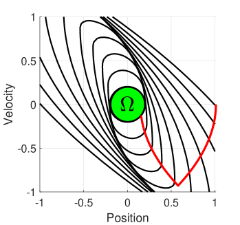
Figure 1: The double integrator example. The zero level set evolution solved at various times shown in black. Direct trajectory generation shown in red. The terminal set, $\Omega$, is shaded green.

The primal-dual method presented in Section III was implemented in MATLAB R2017a on a laptop equipped with an Intel Core i7-7500 CPU running at 2.70 GHz. For all experiments, $100$ time samples were used for the quadrature in $\left(\ref{eq: Generalized Hopf with quadrature}\right)$ and the dual step size was set to $\sigma=\frac{1}{\tau\left\|K\right\|^{2}}$, and $\theta=1$. The initial conditions for all examples is $p^{0}=\bar{p}^{0}=x_{0}$ for the primal variable and $y^{0}=Kp^{0}$ for the dual variable. Note that for some of the examples to follow, the action of the matrix exponential is known in closed form and that can be used for increased computational enhancement. Since in general this is not the case, we used [24] to numerically compute the action of the matrix exponential as to show dimensional scaling properties even for the most general case.

VI-A Double Integrator

We begin with the simple double integrator problem with system $\dot{x}=Ax+Bu$ with

$$A=\left[\begin{array}[]{cc}0&1\\ 0&0\end{array}\right]$$

and

$$B=\left[\begin{array}[]{c}0\\ 1\end{array}\right],$$

where the state $x\in\mathbb{R}^{2}$ is position and velocity. This problem is selected since closed form optimal solutions exist and is low enough dimension to compare the level set evolution to that of grid based numeric techniques such as that in [3, 29]. We consider the control to be constrained to $u\in\left[-1,1\right]$ and implies a control of $\mathcal{C}=\left\{u:\left|u\right|\leq 1\right\}$. After a change of variables $\left(\ref{eq:change of varibles}\right)$, the Hamiltonian becomes

$$H_{z}\left(p,t\right)=\left|\left(-e^{-\left(T-t\right)A}B\right)^{\top}p\right|.$$

We chose the terminal set to be an ellipsoidal with

$$\Omega=\left\{x:\left\langle x,W^{-1}x\right\rangle\leq 1\right\}.$$ (34)

where $W$ is symmetric positive definite. For the initial cost function $J_{x}$, the elements of $W$ are selected such that $\Omega$ is a circle with radius $r=0.2$. The terminal cost function becomes

$$J_{z}\left(z,0\right)=\left\langle z,V\left(0\right)z\right\rangle-1$$

where $V\left(t\right)=e^{\left(T-t\right)A^{\top}}W^{-1}e^{\left(T-t\right)A}$. This gives

$$J_{z}^{\star}\left(p,0\right)=\frac{1}{4}\left\langle p,V\left(0\right)^{-1}p\right\rangle+1.$$ (35)

In this example $\left(\ref{eq:G, for prox}\right)$ becomes

$$G\left(p\right)=\frac{1}{4}\left\langle p,V\left(0\right)^{-1}p\right\rangle-\left\langle z_{0},p\right\rangle+1,$$ (36)

which is quadratic and results in the following proximal point of $G$ at $p$:

$$\left(I+\tau\partial G\right)^{-1}\left(p\right)=\left(I+\frac{1}{2}\tau V\left(0\right)^{-1}\right)^{-1}\left(p+\tau z_{0}\right).$$ (37)

Note that we do not need to compute the inverse of $V\left(0\right)$ since

$$V\left(0\right)^{-1}=e^{-TA}We^{-TA^{\top}}.$$

Likewise, with $F_{i}^{\star}$ defined in $\left(\ref{eq:F_i}\right)$, the proximal points of each $F_{i}^{\star}$ at $y_{i}$ in $\left(\ref{eq:seperable prox}\right)$ is given by

$$\left(I+\sigma\partial F_{i}^{\star}\right)^{-1}\left(y_{i}\right)=\Delta t\,\text{sign}\left(w_{i}\right)\text{min}\left(\left|w_{i}\right|,1\right),$$

where $w_{i}=\frac{y_{i}}{\Delta t}$ and $\text{sign}\left(\beta\right)=1$ if $\beta\geq 0$ and $-1$ otherwise.

We computed the solution to the Hamilton–Jacobi equation at each point on a grid, $\left[-1,1\right]^{2}$, of 50 equally spaced points in each dimension. This was done to average execution time for a large number of initial conditions. The average computational time was $2.1\,ms$ per point on the grid and the zero contours of the value function for ten different times equally spaced on $t\in[0,T^{*}]$ are shown in Figure 1. The value of $T^{*}$ we set as by solving for the minimum time to the zero level set for the initial state $z_{0}=x_{0}=\left(1,0\right)^{\top}$ using the method presented in Section IV. The primal step size was set to $\tau=10$.

The optimal trajectory starting at $z_{0}$ was computed following $\left(\ref{eq:optimal trajectory at sample}\right)$ with

$$\gamma_{z}\left(T^{*}\right)=\frac{\partial}{\partial p}J_{z}^{\star}\left(p^{*},0\right)=\frac{1}{2}V\left(0\right)^{-1}p^{*},$$

since $J_{x}\left(x\right)$ is quadratic. The gradient of the Hamiltonian is

$$\frac{\partial}{\partial p}H_{z}\left(p^{*},t_{k}\right) =-e^{-\left(T^{*}-t_{k}\right)A}B$$

$$\times\text{sign}\left(\left(-e^{-\left(T^{*}-t_{k}\right)A}B\right)^{\top}p^{*}\right).$$

The trajectory as computed in $\left(\ref{eq:optimal trajectory at sample}\right)$ is shown in red in Figure 1.

VI-B Unscented Optimal Control

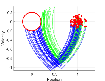
(a) 100 random samples of initial conditions with the existing control formulation. 66 samples reached the goal state and 34 missed.

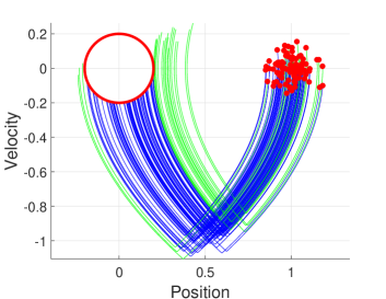
(b) 100 random samples of initial conditions with uncertainty modeled as an unscented control problem. 79 samples reached the goal state and 21 missed.

Figure 2: An example of unscented control applied to a time-optimal double integrator problem with uncertain initial state. Red are samples of the initial states. Blue trajectories are random initial states that reached the goal state and green are trajectories that missed the goal state. Best viewed in color.

We can utilize the favorable dimensional scaling of the proposed methods to generate solutions that are robust to system uncertainty. These uncertainties could be the initial state or system parameters such as mass, lift coefficients, or other properties. The idea is to augment the system to include samples that represent different initial conditions or parameters that share one, common control input. This system forms a tychastic [30] differential equation, since the parameters are fixed, but unknown at run time. The goal is to select a single control so the aggregate cost of all samples is optimized.

For uncertainties that can be modeled as Gaussian, we can choose the samples deterministically with the unscented transform [31], and these samples are typically referred to in literature as sigma points. This transform provides a second-order approximation of the moments of a Gaussian distribution propagated through a nonlinear function. It was developed for state estimation problems and in this context is known as the unscented Kalman filter [32, 33]. Using the unscented transform for sample selection to approximate the tychastic optimal control problem was developed by Ross et al. [34, 35]. The extra state dimensions that result from this technique is not as problematic with proximal splitting as it may be with other methods.

Let $x=\left(\chi^{\left[1\right]},\chi^{\left[2\right]},\ldots,\chi^{\left[2n+1\right]}\right)^{\top}$ , with $\chi^{\left[i\right]}\in\mathbb{R}^{n}$ represent the new state vector augmented by $2n+1$ states generated from the unscented transform and the new system becomes

$$\dot{x}=\left[\begin{array}[]{c}\dot{\chi}_{1}\\ \dot{\chi}_{2}\\ \vdots\\ \dot{\chi}_{2n+1}\end{array}\right]=\left[\begin{array}[]{c}f_{1}\left(\chi^{\left[1\right]},u\right)\\ f_{2}\left(\chi^{\left[2\right]},u\right)\\ \vdots\\ f_{2n+1}\left(\chi^{\left[2n+1\right]},u\right)\end{array}\right],$$

subject to initial condition $z_{0}=x_{0}=\left(\chi_{0}^{\left[1\right]},\chi_{0}^{\left[2\right]},\ldots,\chi_{0}^{\left[2n+1\right]}\right)$. Take for example the problem of uncertainty in initial condition, $x_{0}\sim\mathcal{N}\left(\mu,\Sigma\right)$. As an unscented control problem, the dynamics are the same, so $f_{1}=f_{2}=\cdots=f_{2n+1}=f$, and our augmented system is $\dot{x}=\tilde{A}x+\tilde{B}u$ with

$$\tilde{A}=\left[\begin{array}[]{cccc}A&\cdots&&0\\ \vdots&A&&\vdots\\ &&\ddots\\ 0&\cdots&&A\end{array}\right],$$

and

$$\tilde{B}=\left[\begin{array}[]{c}B\\ B\\ \vdots\\ B\end{array}\right].$$

The initial state becomes $x_{0}=\left\{\chi_{0}^{\left[i\right]}\right\}_{i=1,\ldots,2n+1}$, where each $\chi_{0}^{\left[i\right]}$ is formed by the unscented transform with mean $\mu$ and covariance $\Sigma$. The mean square error of the terminal state relative to some goal state, $\hat{x}_{T}$ is found with the unscented transform by

$$\text{MSE}\approx\sum_{i=1}^{2n+1}w_{m}^{\left[i\right]}\left(\chi_{T}^{\left[i\right]}-\hat{x}_{T}\right)^{\top}\left(\chi_{T}^{\left[i\right]}-\hat{x}_{T}\right),$$ (38)

where $w_{m}$ is the mean weight factor, and $\chi_{T}^{\left[i\right]}$ is the terminal state for the $i$-th unscented sigma point. For this example, we wish to find the minimum time to reach the origin subject to the constraint that the mean square error is less than some threshold $\ell$. This can be found from $\left(\ref{eq:UT recondtructed Cov}\right)$ with

$$\text{MSE}=\mathbb{E}\left[\left(\hat{x}_{T}-x\left(T\right)\right)^{\top}\left(\hat{x}_{T}-x\left(T\right)\right)\right]\leq\ell.$$

We select the origin as the goal with $\hat{x}=\left(0,0\right)^{\top}$, and formulate as an unscented control problem. The trace of the terminal covariance can be represented by the quadratic

$$J\left(z\right)=\left\langle z,V\left(0\right)z\right\rangle-\ell$$ (39)

with $V\left(t\right)=e^{\left(T-t\right)A^{\top}}W^{-1}e^{\left(T-t\right)A}$ and

$$W=\left[\begin{array}[]{ccc}\left(w_{m}^{\left[1\right]}\right)^{-1}I_{2}&\cdots&0\\ \vdots&\ddots&\vdots\\ 0&\cdots&\left(w_{m}^{\left[2n+1\right]}\right)^{-1}I_{2}\end{array}\right],$$

where $I_{2}$ is the $2\times 2$ identity matrix.

Figure 2 shows example trajectories when the initial condition has random perturbations, with $\mu=x_{0}$ and $\Sigma=\pi^{2}I_{2}$, for a double integrator problem. The standard deviation was set to $\pi=0.0667$. If the initial state is exactly what was used to compute the optimal control, then the trajectory generated reaches the goal and is time-optimal. However, if the initial state is perturbed, some trajectories miss the intended goal entirely. In this particular example, it is especially sensitive to perturbations to the “right” in the spatial $x$ direction and is shown in the Figure 2a on the left. Of $100$ random initial states, $34$ miss the goal state. For the resulting $10$ dimensional unscented control problem with $\tau=0.5$, the HJ solutions were found on average $4.0\,ms$ per point. Trajectory samples are shown in the Figure 2a on the right, the number of trajectories that miss the goal is reduced to only $5$.

VI-C Dimensional Scaling

Next we seek to analyze how the proposed method scales with dimension. We can construct a problem similar to that presented in Section VI-B but by selecting samples at random as opposed to using the unscented transform. Constructing a problem in this fashion is something not typically done in practice, but allows us to vary the number of random samples, and hence alter the dimension of the problem in a consistent and uniform way. The initial state for $k$ samples becomes $x_{0}=\left\{\chi_{0}^{\left[i\right]}\right\}_{i=1,\ldots,k}$, where each $\chi_{0}^{\left[i\right]}$ is an independent and identically distributed (iid) random vector drawn according to $\chi_{0}^{\left[i\right]}\sim\mathcal{N}\left(\mu,\Sigma\right)$. To again penalize the trace, the terminal cost function is the same as $\left(\ref{eq:Trace quadratic cost}\right)$ except $W$ is now defined by

$$W=\left[\begin{array}[]{ccc}kI_{2}&\cdots&0\\ \vdots&\ddots&\vdots\\ 0&\cdots&kI_{2}\end{array}\right].$$

Figure 3 shows the average computational time and average iterations to convergence for dimensions ranging from $30$ to $120$. The green line in the figure is the least squares polynomial fit for average computation time in milliseconds. If we let $d$ denote problem dimension for the experiments, the fit is $t_{\text{comp}}=2.382\times 10^{-4}d^{2}+0.0414d+2.598$. Note the extremely small quadratic coefficient.

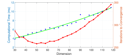
Figure 3: Dimensional scaling properties as described by the experiment in Section VI-C. The blue dots represent average computational time for an experiment and the green line is the least squares polynomial fit to computational time. The red displays average iterations to convergence.

VII Conclusion

Presented is a parallel primal-dual method to solve the Hamilton–Jacobi equation for time-optimal control using the generalized Hopf formula. We empirically showed how the method scales approximately quadratic with dimension, though with small quadratic coefficient. The experiments were shown using Matlab, and simple implementation in a compiled language could provide significant computational improvement. Future work includes increased experimentation with different systems, the use of more advanced quadrature methods, adaptive step sizes, time-varying systems, and state dependent Hamiltonians.

References

- [1] N. P. Osmolovskii, Calculus of Variations and Optimal Control. American Mathematical Society, 1998, vol. 180.
- [2] S. Osher and R. Fedkiw, Level Set Methods and Dynamic Implicit Surfaces. Springer Science & Business Media, 2006, vol. 153.
- [3] I. M. Mitchell, “The flexible, extensible and efficient toolbox of level set methods,” Journal of Scientific Computing, vol. 35, no. 2, pp. 300–329, 2008.
- [4] I. Mitchell, A. M. Bayen, and C. J. Tomlin, “A time-dependent Hamilton-Jacobi formulation of reachable sets for continuous dynamic games,” IEEE Transactions on Automatic Control, vol. 50, no. 7, pp. 947–957, 2005.
- [5] R. E. Bellman, Adaptive Control Processes: A Guided Tour. Princeton University Press, 2015.
- [6] ——, Dynamic Programming. Princeton University Press, 1957, vol. 1, no. 2.
- [7] J. Darbon and S. Osher, “Algorithms for overcoming the curse of dimensionality for certain Hamilton-Jacobi equations arising in control theory and elsewhere,” Research in the Mathematical Sciences, vol. 3, no. 1, p. 19, 2016.
- [8] M. R. Kirchner, R. Mar, G. Hewer, J. Darbon, S. Osher, and Y. T. Chow, “Time-optimal collaborative guidance using the generalized Hopf formula,” IEEE Control Systems Letters, vol. 2, no. 2, pp. 201–206, 2018.
- [9] N. F. Palumbo, R. A. Blauwkamp, and J. M. Lloyd, “Modern homing missile guidance theory and techniques,” Johns Hopkins APL Technical Digest, vol. 29, no. 1, pp. 42–59, 2010.
- [10] T. Goldstein and S. Osher, “The split Bregman method for L1-regularized problems,” SIAM Journal on Imaging Sciences, vol. 2, no. 2, pp. 323–343, 2009.
- [11] Y. T. Chow, J. Darbon, S. Osher, and W. Yin, “Algorithm for overcoming the curse of dimensionality for time-dependent non-convex Hamilton–Jacobi equations arising from optimal control and differential games problems,” Journal of Scientific Computing, pp. 1–27, 2016.
- [12] P. L. Combettes and J.-C. Pesquet, “Proximal splitting methods in signal processing,” in Fixed-point Algorithms for Inverse Problems in Science and Engineering. Springer, 2011, pp. 185–212.
- [13] N. Parikh and S. Boyd, “Proximal algorithms,” Foundations and Trends in Optimization, vol. 1, no. 3, pp. 127–239, 2014.
- [14] A. R. Bryson and Y.-C. Ho, Applied Optimal Control: Optimization, Estimation and Control. CRC Press, 1975.
- [15] L. C. Evans, Partial differential equations. Providence, R.I.: American Mathematical Society, 2010.
- [16] E. Hopf, “Generalized solutions of non-linear equations of first order,” Journal of Mathematics and Mechanics, vol. 14, pp. 951–973, 1965.
- [17] J.-B. Hiriart-Urruty and C. Lemaréchal, Fundamentals of convex analysis. Springer Science & Business Media, 2012.
- [18] A. B. Kurzhanski and P. Varaiya, Dynamics and Control of Trajectory Tubes: Theory and Computation. Springer, 2014, vol. 85.
- [19] I. M. Mitchell, “A toolbox of level set methods,” UBC Department of Computer Science, Tech. Rep. TR-2007-11, 2007.
- [20] A. Chambolle and T. Pock, “A first-order primal-dual algorithm for convex problems with applications to imaging,” Journal of Mathematical Imaging and Vision, vol. 40, no. 1, pp. 120–145, 2011.
- [21] J. H. Mathews and K. D. Fink, Numerical Methods using MATLAB. Prentice Hall, 1999, vol. 3.
- [22] I. M. Ross and M. Karpenko, “A review of pseudospectral optimal control: From theory to flight,” Annual Reviews in Control, vol. 36, no. 2, pp. 182–197, 2012.
- [23] T. Pock and A. Chambolle, “Diagonal preconditioning for first order primal-dual algorithms in convex optimization,” in 2011 IEEE International Conference on Computer Vision (ICCV). IEEE, 2011, pp. 1762–1769.
- [24] A. H. Al-Mohy and N. J. Higham, “Computing the action of the matrix exponential, with an application to exponential integrators,” SIAM Journal on Scientific Computing, vol. 33, no. 2, pp. 488–511, 2011.
- [25] T. Goldstein, M. Li, X. Yuan, E. Esser, and R. Baraniuk, “Adaptive primal-dual hybrid gradient methods for saddle-point problems,” arXiv preprint arXiv:1305.0546, 2013.
- [26] P. L. Lions and J.-C. Rochet, “Hopf formula and multitime Hamilton-Jacobi equations,” Proceedings of the American Mathematical Society, vol. 96, no. 1, pp. 79–84, 1986.
- [27] J. Darbon, “On convex finite-dimensional variational methods in imaging sciences and Hamilton-Jacobi equations,” SIAM Journal on Imaging Sciences, vol. 8, no. 4, pp. 2268–2293, 2015.
- [28] I. M. Ross, A primer on Pontryagin’s principle in optimal control. Collegiate Publishers, 2015.
- [29] I. M. Mitchell and J. A. Templeton, “A toolbox of Hamilton-Jacobi solvers for analysis of nondeterministic continuous and hybrid systems,” in HSCC, vol. 5. Springer, 2005, pp. 480–494.
- [30] J.-P. Aubin, L. Chen, O. Dordan, A. Faleh, G. Lezan, and F. Planchet, “Stochastic and tychastic approaches to guaranteed ALM problem,” Bulletin Français d’Actuariat, vol. 12, no. 23, pp. 59–95, 2012.
- [31] S. J. Julier, “The scaled unscented transformation,” in American Control Conference, 2002. Proceedings of the 2002, vol. 6. IEEE, 2002, pp. 4555–4559.
- [32] S. J. Julier and J. K. Uhlmann, “Unscented filtering and nonlinear estimation,” Proceedings of the IEEE, vol. 92, no. 3, pp. 401–422, 2004.
- [33] S. Thrun, W. Burgard, and D. Fox, Probabilistic Robotics. MIT press, 2005.
- [34] I. M. Ross, R. J. Proulx, and M. Karpenko, “Unscented guidance,” in American Control Conference (ACC), 2015. IEEE, 2015, pp. 5605–5610.
- [35] I. M. Ross, M. Karpenko, and R. J. Proulx, “Path constraints in tychastic and unscented optimal control: Theory, application and experimental results,” in American Control Conference (ACC), 2016. IEEE, 2016, pp. 2918–2923.