Nematic quantum phases in the bilayer honeycomb antiferromagnet

Abstract

The spin$-1/2$ Heisenberg antiferromagnet on the honeycomb bilayer lattice is shown to display a rich variety of semiclassical and genuinely quantum phases, controlled by the interplay between intralayer frustration and interlayer exchange. Employing a complementary set of techniques, comprising spin rotationally invariant Schwinger boson mean field theory, bond operators, and series expansions we unveil the quantum phase diagram, analyzing low-energy excitations and order parameters. By virtue of Schwinger bosons we scan the complete range of exchange parameters, covering both long range ordered as well as quantum disordered ground states and reveal the existence of an extended, frustration induced lattice nematic phase in a range of intermediate exchange unexplored so far.

Frustrated magnets are of great interest to a broad range of sub fields in physics, harboring new quantum states of condensed matter Moessner2006 ; Balents2010 , fueling progress on fundamental paradigms of topological ordering Wen1990 ; Wen2002 ; Kitaev2003 , providing realistic prospects for quantum computing Benjamin2015 ; Riste2015 ; Corcoles2015 and devices for thermal management technologies Zhitomirsky2003 ; Pakhira2017 , inspiring research on ultra cold atomic gases Kim2010 ; Struck2011 , realizing elementary excitations related to Grand Unified Theories (GUT) Castelnovo2008 ; Mengotti2011 ; Hooft1974 , and exhibiting correlations found in soft matter, liquid crystals, and even cosmic strings Jaubert2011 ; Austin1994 . Strong frustration in quantum magnets can ultimately lead to spin liquids, free of any broken symmetries, featuring long-range entanglement, topological order and anyonic excitations Balents2010 ; Savary2016 . Proximate to such liquids, a rich variety of additional exotic quantum matter, including valence bond crystals, also termed lattice nematics Matan2010 , chiral liquids Grohol2005 , multipolar states Damle2006 , and more complex phases compete for stability. Understanding such phases of matter and their interplay is a critically outstanding problem for theory and experiment. In this letter we take a major step forward into this direction and detail the emergence of lattice nematic order in a yet unexplored region of frustrated magnets on bilayer honeycomb lattices.

Recently, frustrated Heisenberg models on single layer honeycomb lattices have become a test-bed for competing spiral order, lattice nematicity and plaquette valence bond states Mulder et al. (2010); Okumura et al. (2010); Wang (2010); Mosadeq et al. (2011); Cabra et al. (2011a); Ganesh et al. (2011a); Albuquerque et al. (2011); Clark et al. (2011); Cabra et al. (2011b); Mezzacapo and Boninsegni (2012); Bishop et al. (2012); Li et al. (2012); Bishop et al. (2013); Gong et al. (2013); Ganesh et al. (2013); Zhu et al. (2013); Zhang and Lamas (2013). This interest has been propelled by the discovery of bismuth oxynitrate, Bi₃Mn₄O₁₂(NO₃) Smirnova et al. (2009), where Mn⁴⁺ ions of spin $3/2$ form honeycomb layers, with both, nearest and next-nearest neighbor antiferromagnetic (AFM) exchange. Early on however, it was noticed that in this compound Mn⁴⁺ ions are grouped into pairs along the c-axis, rendering the structure rather that of a bilayer honeycomb lattice. Despite a significant separation through bismuth atoms, density functional calculation Kandpal and van den Brink (2011) resulted in comparable inter- and intralayer exchange, consistent with experimental findings Matsuda et al. (2010). This has lead to first investigations of bilayer honeycomb systems Ganesh et al. (2011b); Oitmaa and Singh (2012); Zhang et al. (2014); Arlego et al. (2014); Zhang et al. (2016); Bishop and Li (2017); Krokhmalskii et al. (2017). Most of these studies have focused on the stability of the semi-classical phases, extending previous work on the single layer case.

First indications of quantum disordered phases, genuinely related to the bilayer geometry and not present in the single layer case have been provided in a small parameter window in Zhang et al. (2016), following ideas of Bose (1992); Bose and Gayen (1993) and similar works Honecker et al. (2000); Brenig and Becker (2001); Arlego and Brenig (2006); Lamas and Matera (2015); matera-lamas2 . However a complete understanding of the quantum phase diagram of the bilayer is missing. Therefore, in this letter we provide a comprehensive analysis of the quantum phases of the frustrated Heisenberg model on the honeycomb bilayer over a wide range of coupling strengths, including in particular the intermediate regime, where both, the interlayer exchange and intralayer frustration are comparable to the intralayer first neighbor couplings. This part of the phase diagram has remained largely unexplored, representing a challenge for most of the existing state-of-the-art numerical techniques. Here, by means of a combination of methods, among which Schwinger Bosons stand out for their ability to explore the full quantum phase diagram and to treat on equal footing quantum and semi-classical states, we unveil a rich structure of phases, where the interplay of frustration and interlayer coupling is most essential, destroying magnetic order and giving rise to exotic phases. Most noteworthy, we will provide evidence for a new lattice nematic phase in the intermediate coupling regime.

The model we consider is shown in Fig. 1. Its Hamiltonian reads

$$H=\sum_{i,l,m}J^{(l,m)}_{i}\vec{\bf{S}}_{l}(\vec{r})\cdot\vec{\bf{S}}_{m}(\vec{r}+\vec{e}_{i}),$$ (1)

$\vec{r}$ and $\vec{e}_{i}$ label sites and primitive vectors of the triangular Bravais lattice. $\vec{\bf{S}}_{l}(\vec{r})$ are spin operators at basis sites $\vec{r}$, $l{=}1...4$ of the bilayer. The couplings $J^{(l,m)}_{i}$ are non-zero, with values $J_{\bot}$, $J_{1}$ and $J_{2}$ as depicted in Fig. 1.

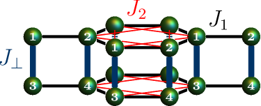
Figure 1: (Color online) Schematic representation of the model. The sites (green spheres) in each unit cell are labeled from 1 to 4. Bold vertical blue lines indicate $J_{\bot}$ interlayer couplings, whereas thin black and red lines indicate $J_{1}$ and $J_{2}$ first and second nearest neighbors, respectively.

Before describing our calculations, we focus on the main results, summarized in Fig. 2A. On the classical level, $S\rightarrow\infty$, and in the single plane limit, i.e. at $J_{\bot}=0$, there are two phases. Néel order for $J_{2}/J_{1}<1/6$ and spiral order for $J_{2}/J_{1}>1/6$. Allowing for interlayer coupling this single transition point extends into a line, independent of $J_{\bot}$. Quantum fluctuations lead to new non-classical intermediate phases and renormalize the Néel and spiral phases. Previous studies Zhang and Lamas (2013) have identified continuous transitions into two frustration induced genuine quantum phases. A gapped spin liquid (GSL) phase, preserving all lattice symmetries for $0.2075\lesssim J_{2}/J_{1}\lesssim 0.3732$ and a staggered-dimer lattice nematic phase (VBC1) which maintains the SU(2) spin rotational and lattice translational symmetries, but breaks $Z_{3}$ symmetry, corresponding to $2\pi/3$ rotations around an axis perpendicular to the plane for $0.3732\lesssim J_{2}/J_{1}\lesssim 0.398$. Another limiting case is $J_{\bot}\rightarrow\infty$. Here an interlayer dimer product phase (IDP) is formed.

Connecting these two limits, the interplay between the interlayer couplings $J_{\bot}$ and the frustration $J_{2}$ reveals the complex phase diagram we find in Fig. 2A. Starting from the limit of decoupled planes, we consider the semiclassical Néel and spiral phases first. Figure 2A shows, that small interlayer couplings extend each of their windows of stability along the $J_{2}$ direction, leading even to a region of competition. However for sufficiently large $J_{\bot}$ the semiclassical phases recess and are suppressed in favor of the IDP. Regarding the GSL and VBC1 phases, interlayer coupling has a dramatic consequence, suppressing them very rapidly, reentering semiclassical phases at finite $J_{\bot}$. Finally, the Néel-to-IDP is direct. This is not so for the Spiral-to-IPD transition. In fact we find yet another lattice nematic region (VBC2) which intervenes. To the best of our knowledge, this has not been observed before.

Next we detail how to arrive at our main result, i.e. Fig. 2, using three complementary techniques, namely, Schwinger bosons mean field theory (SBMFT)Cabra et al. (2011a), Bond operators (BO)Sachdev and Bhatt (1990) and series expansions (SE) Knetter and Uhrig (2000). While being a mean field approach, primarily gauged towards bosonic fixed point models, SBMFT is superior in addressing on equal footing both semi-classical as well as genuinely quantum phases, allowing to scan all of Eq. (1)’s parameter space. The other two methods are best suited to obtain additional information, for large interlayer coupling (BO), and for weak frustration (SE).

SBMFT.— Here, spin operators are represented by two bosons $\vec{\mathbf{S}}_{l}(\vec{r})=$ $\frac{1}{2}\vec{\mathbf{b}}_{l}^{{\dagger}}(\vec{r})\cdot\vec{\sigma}\cdot\vec{\mathbf{b}}_{l}(\vec{r})$ Auerbach and Arovas (1988); Auerbach (1994); Auerbach and Arovas (2011), where ${\vec{\bf b}^{\dagger}_{l}(\vec{r})}\!=\!({\bf b}^{\dagger}_{l,\uparrow}(\vec{r}),{\bf b}^{\dagger}_{l,\downarrow}(\vec{r}))$ is a spinor, $\vec{\sigma}$ are the Pauli matrices, and $\sum_{\sigma}\mathbf{b}^{{\dagger}}_{l,\sigma}(\vec{r})\mathbf{b}_{l,\sigma}(\vec{r})\!=\!2S$ is a local constraint. Using the rotationally invariant representation Zhang and Lamas (2013); Cabra et al. (2011a, b); Ceccatto et al. (1993); Trumper et al. (1997); Flint and Coleman (2009); Mezio et al. (2011); Messio et al. (2012, 2013), we define two $SU(2)$ invariants $\mathbf{A}_{lm}(\vec{x},\vec{y})=\frac{1}{2}\sum_{\sigma}\sigma\mathbf{b}_{l,\sigma}(\vec{x})\mathbf{b}_{m,-\sigma}(\vec{y})$ and $\mathbf{B}_{lm}(\vec{x},\vec{y})=\frac{1}{2}\sum_{\sigma}\mathbf{b}^{{\dagger}}_{l,\sigma}(\vec{x})\mathbf{b}_{m,-\sigma}(\vec{y})$, where the former generates a spin singlet between sites $l$ and $m$, and the latter a coherent hopping of the Schwinger bosons. At the mean field level, the exchange follows as $\langle(\vec{\mathbf{S}}_{l}(\vec{x})\cdot\vec{\mathbf{S}}_{m}(\vec{y}))_{MF}\rangle=|B_{lm}(\vec{x}-\vec{y})|^{2}-|A_{lm}(\vec{x}-\vec{y})|^{2},$ with $A^{*}_{lm}(\vec{x}-\vec{y})=\langle\mathbf{A}^{{\dagger}}_{lm}(\vec{x},\vec{y})\rangle$ and $B^{*}_{lm}(\vec{x}-\vec{y})=\langle\mathbf{B}^{{\dagger}}_{lm}(\vec{x},\vec{y})\rangle$. These equations are solved self-consistently taking into account the constraint in the number of bosons $B_{ll}(\vec{R}=\vec{0})=4N_{c}S$, whith $N_{c}$ representing the total number of unit cells and $S$ the spin strength Cabra et al. (2011a); Zhang and Lamas (2013).

After solving the mean-field equations on finite but large lattices we primarily extract the extrapolation of the elementary excitation gap $\Delta$. This is used to classify magnetic phases, for which $\Delta$ has to be zero. If $\Delta\neq 0$, Bose condensation cannot occur and the phase is quantum disordered. We can also obtain the real space spin correlation function $C_{l}$ and magnetization $m_{l}$ note:corr . Lattice nematic phases, which preserve the lattice translational invariance, but break $Z_{3}$ lattice symmetry have come under scrutiny early on in single layer honeycomb systems. These imply a nonzero order parameter $\rho=\frac{4}{3}|(\langle\vec{\mathbf{S}}_{1}(\vec{r})\cdot\vec{\mathbf{S}}_{2}(\vec{r})\rangle+e^{i2\pi/3}\langle\vec{\mathbf{S}}_{1}(\vec{r})\cdot\vec{\mathbf{S}}_{2}(\vec{r}+\vec{e}_{1})\rangle+e^{i4\pi/3}\langle\vec{\mathbf{S}}_{1}(\vec{r})\cdot\vec{\mathbf{S}}_{2}(\vec{r}-\vec{e}_{2})\rangle)|$ Okumura et al. (2010); Mulder et al. (2010). Here we have investigated this order parameter over all of the parameter space of Fig. 2A.

To clarify the procedure we detail our SBMFT results along the two paths (a-d), at $J_{2}=0.3$ and (f-g), at $J_{2}=0.38$ in a representative part of the phase diagram, depicted in Fig. 2B. The corresponding evolution of $\Delta$ (connected red dots) and $\rho$ (connected black dots) are shown in Fig. 2C and 2D for the paths (a-d) and (f-g), respectively.

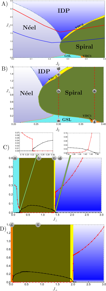
Figure 2: (Color online) Panel (A): the different colored regions identify the phases of model (1) in $J_{2}-J_{\bot}$ plane (in units of $J_{1}$) determined by SBMF. The blue and red lines represent the border of the IDP phase predicted by SE and BO respectively. Panel (B): Zoom of the phase diagram where two paths along $J_{\bot}$, for $J_{2}=0.3$ and $J_{2}=0.38$ are indicated with red dashed lines. Lower panels (C-D), depict the evolution of the gap (connected red dots) and the $Z_{3}$ directional symmetry-breaking order parameter $\rho$ (connected black dots), along the mentioned paths.

We start in the blue-light phase around point (a), where panel C) features a finite gap and unbroken $Z_{3}$ symmetry. This identifies the GSL phase. As $J_{\bot}$ increases from zero, the gap rapidly decreases and closes simultaneously with $\rho$ growing finite. A blowup of this is shown in the left upper inset of Fig. 2C. This behavior is consistent with a spiral phase, which is gapless and breaks $Z_{3}$ symmetry. As $J_{\bot}$ increases further, $\rho$ runs through a maximum and decreases up to a point where $\Delta\neq 0$ again. In stark contrast to the GSL however a narrow yellow region of broken $Z_{3}$ symmetry and gapful behavior surfaces around point (c). This characterizes the lattice nematic phase (VBC2). Right upper inset of Fig. 2C shows a blowup of this region. Very different than the VBC1 phase, VBC2 can be found in a much larger range of parameters running all along the upper spiral phase boundary. Finally, entering the blue region around point (d), there is a near 1st order jump to rather large values of $\Delta$ where $\rho$ turns zero, restoring $Z_{3}$ symmetry. This is consistent with the IDP, adiabatically connecting to the limit of decoupled dimers at $J_{\bot}=\infty$

Turning to the second path (points f and g), it is obvious from Fig. 2D, that the phases corresponding to point (g) is identical with the corresponding one at point (b). However, different from the GSL at (a), the phase VBC1 around (f) displays a behavior of $\Delta$ and $\rho$ identical to point (c), i.e. a lattice nematic. We cannot exclude the existence of observables beyond our study which allow for further discrimination between VBC1 and VBC2.

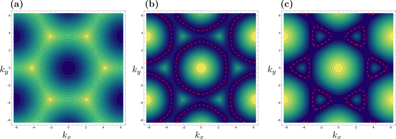
Figure 3: (Color online) Contour plot corresponding to the Bond operator boson dispersion close to condensation for (a): $J_{2}/J_{1}=0.1$, (b) $J_{2}/J_{1}=0.4$ and (c) $J_{2}/J_{1}=0.6$. Red dashed lines correspond to curves in the k space determining the classical manifold of spiral ground states.

Series Expansion and Bond Operator Approach.— For a complementary analysis of the evolution of the quantum disordered phases, starting from the limit of decoupled dimers, $J_{\bot}\rightarrow\infty$, we use both, series expansion (SE) Oitmaa et al. (2006) and bond operator theory (BOT) Chubukov (1989); Chubukov and Jolicoeur (1991); Sachdev and Bhatt (1990). In BOT, spins at the vertices of each dimer are written as $S^{\alpha}=(\pm s^{\dagger}t_{\alpha}\pm t^{\dagger}s-\sum_{\beta,\gamma}i\varepsilon_{\alpha\beta\gamma}t_{\beta}^{\dagger}t_{\gamma}^{\phantom{\dagger}})/2$, with the constraint $s^{\dagger}s+\sum_{\alpha}t_{\alpha}^{\dagger}t_{\alpha}^{\phantom{\dagger}}=1$, where $s^{\dagger}(t_{\alpha}^{\dagger})$ create singlet(triplet) states of the dimer, and $\alpha=1,2,3$ labels the triplet multiplet. BOT maps the spin model onto an interacting Bose gas, for which several schemes of treatment have been proposed Sachdev and Bhatt (1990); Chubukov (1989); Chubukov and Jolicoeur (1991); Kotov1998 ; Matsumoto2002 . Here we use the Holstein-Primakoff (HP) approximation Chubukov (1989); Chubukov and Jolicoeur (1991), where $s^{(\dagger)}$ is replaced by a $C$-number and $s=(1-\sum_{\alpha}t_{\alpha}^{\dagger}t_{\alpha}^{\phantom{\dagger}})^{1/2}$ is expanded to obtain a quadratic triplon Hamiltonian. Standard Bogoliubov diagonalization yields a ground state energy per unit cell of $E={-}\frac{9}{4}+\frac{3}{4N}\sum_{k,\pm}[1\pm\epsilon_{\pm}(k)]^{1/2}$, with the triplon dispersions $\epsilon_{\pm}(k)=$ $\frac{J_{1}}{J_{\bot}}[3{+}$ $2\cos(k_{x})+4\cos(k_{x}/2)$ $\cos(\sqrt{3}k_{y}/2)]^{1/2}$ $\pm 2\frac{J_{1}}{J_{\bot}}(\cos(k_{x})+$ $2\cos(k_{x}/2)$ $\cos(\sqrt{3}k_{y}/2))$. At $J_{1}{=}J_{2}{=}0$, and for the latter one recovers the bare singlet-triplet gap $\Delta=J_{\bot}$, and for the former $E={-}3J_{\bot}/4$ consistent with a bare singlet.

For SE we use the continuous unitary transformation (CUT) method Wegner (1994); Knetter and Uhrig (2000); Arlego and Brenig (2011, 2008, 2007, 2006) starting from the limit of decoupled dimers. This method allows to obtain analytical expressions for the ground state energy and the dispersion of the elementary triplon excitations of the IDP versus $J_{1,2}/J_{\bot}$. We have evaluated these up to $O(4)$. Their rather lengthy expressions are detailed elsewhere SuppMat .

In Fig. 2A we show the critical lines of the gap closure of the triplon dispersion of the IDP obtained from both, BOT-HP (red solid) and SE-CUT (blue dotted line). Clearly, contrasting them with regions of magnetic ordering obtained from SBMFT, the general trend, i.e. the breakdown of magnetic order versus $J_{2}$ and $J_{\bot}$ is fully consistent with the IDP gap closure. Quantitatively however, comparing SBMFT and BOT-HP to SE-CUT, the latter predicts a smaller range of stability for semiclassical phases. Since the former two are mean-field theories, such a tendency to prefer ordered phases is a well known shortcoming. In fact, SE-CUT locates the IDP-Néel transition at $J_{\bot}\simeq 1.6$ for $J_{2}=0$ in Fig. 2A, in excellent agreement with quantum Monte-Carlo calculations Ganesh et al. (2011b), and moreover SE-CUT is rather close to coupled-cluster results for finite, but small $J_{2}\lesssim 0.2$ Bishop and Li (2017). For larger $J_{2}$ the CUT-SE bcomes less reliable and we remain with only BOT-HP to compare to within the IDP.

Finally, we comment on the location in $\vec{k}$-space of Bose condensation within the BOT-HP, as compared to the classical magnetic pitch vector $\vec{Q}$ of the bilayer at $S\rightarrow\infty$. As mentioned previously, the latter is independent of $J_{\bot}$, comprising a Néel state for each plane for $0<J_{2}/J_{1}<1/6$ and for $1/6<J_{2}/J_{1}$ a set of classically degenerate coplanar spiral ground states with $\vec{S}_{l}(\vec{r})=(-1)^{l}S[\cos(\vec{Q}\cdot\vec{r}+\theta_{l})\hat{i}+\sin(\vec{Q}\cdot\vec{r}+\theta_{l})\hat{j}]$, where the pitch vector lies on the closed curve $\cos(Q_{x})+\cos(-Q_{x}/2+\sqrt{3}Q_{y}/2)+\cos(Q_{x}/2+\sqrt{3}Q_{y}/2)+3/2=(J_{1}/J_{2})^{2}/8$, and the phase $\theta_{i}$ obeys $\theta_{1,2}=\pi+\theta_{3,4}$ Mulder et al. (2010). Comparing this now, to the critical wave vector $\vec{Q}$ for Bose condensation within the BOT-HP, we first have $\vec{Q}=(0,0)$ corresponding to a Néel order for $J_{2}<\frac{1}{6}$. For $J_{2}>\frac{1}{6}$, condensation does not occur at a single point, but on lines in $\vec{k}$-space. Remarkably, these are identical to those from the classical states. This is illustrated in Fig. 3(a-c), where we plot contours of the boson dispersion close to condensation at $J_{2}=0.1,0.4$ and $0.6$ and incorporate the degenerate classical spiral pitch vector locations by red dashed lines. In turn, while quantum fluctuations may modify such agreement, it is nevertheless interesting to realize that BOT-HP provides some guidance as to the type of semiclassical phase to emerge upon gap closure.

In conclusion, the interplay between intralayer frustration and interlayer exchange allows for a rich variety of classical and quantum disordered phases to compete for stability in the bilayer honeycomb antiferromagnet. In this letter, evidence for these phases has been provided over a wide range of coupling constants using three complementary methods, yielding consistent results. Most noteworthy, at intermediate coupling, we have discovered a new lattice nematic phase, which exists in a region of parameter space substantially larger than similar phases observed previously in the model at small interlayer coupling. While we have carried out our analysis on a spin-$1/2$ model, our findings may be relevant to understand the absence of magnetic order in the spin-$3/2$ honeycomb bilayer materials Bi₃Mn₄O₁₂(NO₃) , where first principle calculations suggest exchange paths identical to our microscopic model and to be all of similar magnitude.

Acknowledgments: C.A.L gratefully acknowledges the support of NVIDIA Corporation. C.A.L. and M.A. are supported by CONICET (PIP 1691) and ANPCyT (PICT 2013-0009). H.Z. thanks Lu Yu for fruitful discussions, and the Institute of Physics, Chinese Academy of Sciences for financial support. Work of W.B. has been supported in part by the DFG through SFB 1143. W.B. also acknowledges kind hospitality of the PSM, Dresden.

References

- (1) R. Moessner and A.P. Ramirez, Phys. Today 59, 24 (2006).
- (2) L. Balents, Nature 464, 199 (2010).
- (3) X.-G. Wen, Int. J. Mod. Phys. B, 04, 239 (1990).
- (4) X.-G. Wen, Phys. Rev. B 65, 165113 (2002).
- (5) A. Kitaev, Ann. Phys. (N.Y.) 303, 2 (2003).
- (6) S. Benjamin and J. Kelly, Nat. Mater. 14, 561 (2015).
- (7) D. Ristè, S. Poletto, M.-Z. Huang, A. Bruno, V. Vesterinen, O.-P. Saira, and L. DiCarlo, Nat. Commun. 6, 7983 (2015).
- (8) A. D. Córcoles, E. Magesan, S. J. Srinivasan, A. W. Cross, M. Steffen, J. M. Gambetta, and J. M. Chow, Nat. Commun. 6, 7979 (2015).
- (9) M. E. Zhitomirsky, Phys. Rev. B 67, 104421 (2003).
- (10) S. Pakhira, C. Mazumdar, R. Ranganathan, and M. Avdeev, Nature Sci. Rep. 7, 7367 (2017).
- (11) K. Kim, M.-S. Chang, S. Korenblit, R. Islam, E. E. Edwards, J. K. Freericks, G.-D. Lin, L.-M. Duan, and C. Monroe, Nature 465, 590 (2010).
- (12) J. Struck, C. Ölschläger, R. L. Targat, P. Soltan-Panahi, A. Eckardt, M. Lewenstein, P. Windpassinger, and K. Sengstock, Science 333, 996 (2011).
- (13) G. ’t Hooft, Nucl. Phys. B 79 276 (1974).
- (14) C. Castelnovo, R. Moessner, and S. L. Sondhi, Nature 451, 42 (2008)
- (15) E. Mengotti, L. J. Heyderman, A. F. Rodríguez, F. Nolting, R. V. Hügli, and H.-B. Braun, Nat. Phys. 7 68 (2011).
- (16) L. D. C. Jaubert, M. Haque, and R. Moessner, Phys. Rev. Lett. 107, 177202 (2011).
- (17) D. Austin, E. J. Copeland, and R. J. Rivers, Phys. Rev. D 49, 4089 (1994).
- (18) L. Savary and L. Balents, Rep. Prog. Phys. 80, 016502 (2017).
- (19) K. Matan, T. Ono, Y. Fukumoto, T. J. Sato, J. Yamaura, M. Yano, K. Morita, and H. Tanaka, Nat. Phys. 6, 865 (2010).
- (20) D. Grohol, K. Matan, J.-H. Cho, S.-H. Lee, J. W. Lynn, D. G. Nocera, and Y. S. Lee, Nat. Mater. 4, 323 (2005).
- (21) K. Damle and T. Senthil, Phys. Rev. Lett. 97, 067202 (2006).
- Mulder et al. (2010) A. Mulder, R. Ganesh, L. Capriotti, and A. Paramekanti, Phys. Rev. B 81, 214419 (2010).
- Okumura et al. (2010) S. Okumura, H. Kawamura, T. Okubo, and Y. Motome, J. Phys. Soc. Jpn. 79, 114705 (2010).
- Wang (2010) F. Wang, Phys. Rev. B 82, 024419 (2010).
- Mosadeq et al. (2011) H. Mosadeq, F. Shahbazi, and S. Jafari, Journal of Physics: Condensed Matter 23, 226006 (2011).
- Cabra et al. (2011a) D. C. Cabra, C. A. Lamas, and H. D. Rosales, Phys. Rev. B 83, 094506 (2011a).
- Ganesh et al. (2011a) R. Ganesh, D. Sheng, Y.-J. Kim, and A. Paramekanti, Phys. Rev. B 83, 144414 (2011a).
- Albuquerque et al. (2011) A. F. Albuquerque, D. Schwandt, B. Hetényi, S. Capponi, M. Mambrini, and A. M. Läuchli, Phys. Rev. B 84, 024406 (2011).
- Clark et al. (2011) B. Clark, D. Abanin, and S. Sondhi, Phys. Rev. Lett. 107, 087204 (2011).
- Cabra et al. (2011b) D. Cabra, C. Lamas, and H. Rosales, Mod. Phys. Lett. B 25, 891 (2011b).
- Mezzacapo and Boninsegni (2012) F. Mezzacapo and M. Boninsegni, Phys. Rev. B 85, 060402(R) (2012).
- Bishop et al. (2012) R. F. Bishop, P. H. Y. Li., D. J. J. Farnell, and C. E. Campbell, J. Phys.: Condens. Matter 24, 236002 (2012).
- Li et al. (2012) P. H. Y. Li, R. F. Bishop, D. J. J. Farnell, and C. E. Campbell, Phys. Rev. B 86, 144404 (2012).
- Bishop et al. (2013) R. F. Bishop, P. H. Y. Li, D. J. J. Farnell, and C. E. Campbell, J. Phys.: Condens. Matter 25, 306002 (2013).
- Gong et al. (2013) S.-S. Gong, D. Sheng, O. I. Motrunich, and M. P. Fisher, Phys. Rev. B 88, 165138 (2013).
- Ganesh et al. (2013) R. Ganesh, J. van den Brink, and S. Nishimoto, Phys. Rev. Lett. 110, 127203 (2013).
- Zhu et al. (2013) Z. Zhu, D. A. Huse, and S. R. White, Phys. Rev. Lett. 110, 127205 (2013).
- Zhang and Lamas (2013) H. Zhang and C. Lamas, Phys. Rev. B 87, 024415 (2013).
- Smirnova et al. (2009) O. Smirnova, M. Azuma, N. Kumada, Y. Kusano, M. Matsuda, Y. Shimakawa, T. Takei, Y. Yonesaki, and N. Kinomura, Journal of the American Chemical Society 131, 8313 (2009).
- Kandpal and van den Brink (2011) H. C. Kandpal and J. van den Brink, Physical Review B 83, 140412 (2011).
- Matsuda et al. (2010) M. Matsuda, M. Azuma, M. Tokunaga, Y. Shimakawa, and N. Kumada, Phys. Rev. Lett. 105, 187201 (2010).
- Ganesh et al. (2011b) R. Ganesh, S. V. Isakov, and A. Paramekanti, Phys. Rev. B 84, 214412 (2011b).
- Oitmaa and Singh (2012) J. Oitmaa and R. Singh, Phys. Rev. B 85, 014428 (2012).
- Zhang et al. (2014) H. Zhang, M. Arlego, and C. A. Lamas, Phys. Rev. B 89, 024403 (2014).
- Arlego et al. (2014) M. Arlego, C. A. Lamas, and H. Zhang, J. Phys.: Conf. Ser. 568, 042019 (2014).
- Zhang et al. (2016) H. Zhang, C. A. Lamas, M. Arlego, and W. Brenig, Phys. Rev. B 93, 235150 (2016).
- Bishop and Li (2017) R. F. Bishop and P. H. Y. Li, Phys. Rev. B 95, 134414 (2017).
- Krokhmalskii et al. (2017) T. Krokhmalskii, V. Baliha, O. Derzhko, J. Schulenburg, and J. Richter, Phys. Rev. B 95, 094419 (2017).
- Bose (1992) I. Bose, Phys. Rev. B 45, 13072 (1992).
- Bose and Gayen (1993) I. Bose and S. Gayen, Phys. Rev. B 48, 10653(R) (1993).
- Honecker et al. (2000) A. Honecker, F. Mila, and M. Troyer, Eur. Phys. J. B 15, 227 (2000).
- Brenig and Becker (2001) W. Brenig and K. W. Becker, Phys. Rev. B 64, 214413 (2001).
- Arlego and Brenig (2006) M. Arlego and W. Brenig, Eur. Phys. J. B 53, 193 (2006).
- Lamas and Matera (2015) C. A. Lamas and J. M. Matera, Phys. Rev. B 92, 115111 (2015).
- (55) J.M. Matera, C.A. Lamas, J. Phys.: Condens. Matter 26 (2014) 326004
- Sachdev and Bhatt (1990) S. Sachdev and R. N. Bhatt, Phys. Rev. B 41, 9323 (1990).
- Knetter and Uhrig (2000) C. Knetter and G. S. Uhrig, The European Physical Journal B-Condensed Matter and Complex Systems 13, 209 (2000).
- Auerbach and Arovas (1988) A. Auerbach and D. P. Arovas, Phys. Rev. Lett. 61, 617 (1988).
- Auerbach (1994) A. Auerbach, Interacting Electrons and Quantum Magnetism (Springer-Verlag, New York, 1994).
- Auerbach and Arovas (2011) A. Auerbach and D. P. Arovas, in Introduction to Frustrated Magnetism (Springer, 2011).
- Ceccatto et al. (1993) H. Ceccatto, C. Gazza, and A. Trumper, Phys. Rev. B 47, 12329 (1993).
- Trumper et al. (1997) A. Trumper, L. Manuel, C. Gazza, and H. Ceccatto, Phys. Rev. Lett. 78, 2216 (1997).
- Flint and Coleman (2009) R. Flint and P. Coleman, Physical Review B 79, 014424 (2009).
- Mezio et al. (2011) A. Mezio, C. Sposetti, L. Manuel, and A. Trumper, Eur. Phys. Lett. 94, 47001 (2011).
- Messio et al. (2012) L. Messio, B. Bernu, and C. Lhuillier, Phys. Rev. Lett. 108, 207204 (2012).
- Messio et al. (2013) L. Messio, C. Lhuillier, and G. Misguich, Phys. Rev. B 87, 125127 (2013).
- (67) For the use of correlations and staggered magnetization to clasify magnetic phases see for example Phys. Rev. B 83, 094506 (2011).
- Oitmaa et al. (2006) J. Oitmaa, C. Hamer, and W. Zheng, Series expansion methods for strongly interacting lattice models (Cambridge University Press, 2006).
- Chubukov (1989) A. V. Chubukov, JETP Lett. 49, 129 (1989).
- Chubukov and Jolicoeur (1991) A. V. Chubukov and T. Jolicoeur, Phys. Rev. B 44, 12050(R) (1991).
- (71) V. N. Kotov, O. Sushkov, Zheng Weihong, and J. Oitmaa, Phys. Rev. Lett. 80, 5970 (1998).
- (72) M. Matsumoto, B. Normand, T. M. Rice, and M. Sigrist, Phys. Rev. Lett. 89, 077203 (2002).
- Wegner (1994) F. Wegner, Ann. Phys. 506, 77 (1994).
- Arlego and Brenig (2011) M. Arlego and W. Brenig, Phys. Rev. B 84, 134426 (2011).
- Arlego and Brenig (2008) M. Arlego and W. Brenig, Phys. Rev. B 78, 224415 (2008).
- Arlego and Brenig (2007) M. Arlego and W. Brenig, Phys. Rev. B 75, 024409 (2007).
- (77) The explicit form of these expressions is impractical to be presented here in written form, but they are available in the supplemental material.