Robust Detection of Covariate-Treatment Interactions in Clinical Trials

Abstract

Detection of interactions between treatment effects and patient descriptors in clinical trials is critical for optimizing the drug development process. The increasing volume of data accumulated in clinical trials provides a unique opportunity to discover new biomarkers and further the goal of personalized medicine, but it also requires innovative robust biomarker detection methods capable of detecting non-linear, and sometimes weak, signals. We propose a set of novel univariate statistical tests, based on the theory of random walks, which are able to capture non-linear and non-monotonic covariate-treatment interactions. We also propose a novel combined test, which leverages the power of all of our proposed univariate tests into a single general-case tool. We present results for both synthetic trials as well as real-world clinical trials, where we compare our method with state-of-the-art techniques and demonstrate the utility and robustness of our approach.

Keywords: Random Walks, Statistical Test, Personalized Medicine, Biomarker Selection, Drug Development

1 Introduction

Designing new and efficient therapies is a long and ever more costly process, with less than ten percent of new treatments entering Phase I finally being approved by the FDA and commercialized [1, 2]. One of the major challenges for the improvement of drug development is to better understand how drugs interact with patients, particularly for treatments displaying heterogeneous responses. Therefore, conducting a detailed analysis of clinical trial data is critical to find subgroups of patients with higher benefit-risk ratio or to understand why a drug does not work on some sub-population to improve existing therapeutic strategies.

Moreover, understanding the relationships of patient descriptors which compose the most responsive cross-section of the population is of great importance when planning a Phase III trial, for salvaging failed trials, or accelerating advances in personalized medicine. This process of biomarker identification is critical to detect sub-groups within a given indication, but, as shown recently for immunotherapies, can also provide the basis for pan-indication drug approval [3].

Identifying these patient subgroups, and understanding the descriptors, or covariates, which distinguish them, is the domain of subgroup analysis. This field of research has a long history in clinical biostatistics [4, 5, 6], and requires a very careful and rigorous methodological approach [7], both for confirmatory or exploratory analysis, due to multiplicity, reproducibility, and false detection issues. Furthermore, subgroup analysis has garnered even more attention recently from the pharmaceutical community with both the advent of cheap and extensive genomic measurements as well as the dawning of the era of so-called big-data. Now that incredibly detailed patient characterizations are available, the problem of subgroup identification has shifted from careful statistical analysis of select covariates, to data-mining and machine learning approaches. While the number of features is increasing by several order of magnitudes, the number of patients remains typically the same, which makes the statistical challenge even more difficult. Therefore, effective clinical trial data analysis requires highly sensitive tools capable of detecting covariate-response associations from noisy and weak treatment response measurements, including discontinuous and non-monotonic interactions, without inflating the Type-I error rate. Indeed, false positive detection is a major caveat in subgroup analysis [7], and controlling Type-I error is a crucial requirement for any reliable methodology. These tools can be used as a pre-processing step, pruning out insignificant covariates which might obfuscate accurate subgroup identification. They can also enable investigators to rank covariates by significance so as to focus laboratory studies to a few of the most promising biological pathways.

Many methods have been proposed for the detection of covariate-treatment interaction. In particular, we note modified outcome regression [8], outcome weighted learning [9], and change-point detection [10] methods as state-of-the art techniques which are useful in constructing baseline comparisons, as we do in this work. We refer the reader to the recent review of Lipkovich et al. [11], where the authors review various methodologies ranging from classic statistical approaches to more sophisticated machine learning methods. On the one hand, well-founded and analytically rich statistical techniques provide rigorous estimates of Type-I error, but often miss complex, non-linear interactions. On the other hand, machine learning approaches allow for the detection of these complex, and sometimes non-monotonic, interactions. However, in general they fail to provide a proper estimate of Type-I error for the impact of individual covariates; they do not possess the characteristics common to proper statistical tests. Thus, we note a lack of methods which take the best of both worlds, offering high sensitivity for interactions with complex dependencies, while also providing rich statistical analysis and a controlled Type-I error rate.

To address this shortfall, we propose a new series of statistical tests, each of which is designed to detect particular structures in the treatment response signal which are often observed in actual clinical trial data. The proposed tests are constructed from a cumulative process on the effect size obtained by ranking patients according to a given covariate. These processes characterize the complex dependency structure of the covariate-treatment effect. We introduce several observables which capture various facets of these interactions, going beyond a simple process maximum estimate, as used in [10]. When possible, we derive theoretical estimates to compute $p$-values thresholds characterizing Type-I error, and when not possible, we propose a Monte-Carlo sampling procedure. We also present a new combined test which leverages the power of all our proposed individual tests to provide robust detection of significant covariates, while also providing fine-grained control over the Type-I error rate. Our novel combined test compares favorably to existing state-of-the-art procedures, serving as an effective tool for the exploration of clinical trial data. We evaluate our approach on both synthetic and real clinical trial datasets. For the purpose of this work, we have also created a synthetic benchmark that captures many “corner cases”, i.e. parameter regimes where existing methods reveal their limitations. These benchmarks may prove useful for other researchers to evaluate their methods.

The paper is organized as follows. In Sec. 2, we present the treatment-response model and introduce some notations. Next, in Sec. 3, we review the current state-of-the-art in covariate-response correlation analysis and covariate selection. Subsequently, in Sec. 4.1, we demonstrate a simple correction based on treatment response correlations which addresses many variance issues observed in current techniques. Then, in Sec. 4.2, we present our novel individual cumulative response tests based on null-tests against Brownian motion, each of which is tailored to different features in the measured treatment response. Finally, in Sec. 4.3 we present an approach to merge these individual cumulative tests into a single combined test which is able to retain the performance of the individual tests while being robust to a priori unknown treatment response curves. To validate our approach, we present two numerical analyses. In our first synthetic analysis, reported in Sec. 5, we report objective results of significant covariate detection performance over a wide range of different treatment response models. In our second analysis, reported in Sec. 6, we take three real-world clinical trial datasets and report the significant variables discovered by our method. Finally, we conclude in Sec. 7 with a discussion of the applicability of our approach and possible avenues for future work.

2 Drug response model

Let us now describe the mathematical framework of the drug response model. The drug response model characterizes the observed outcome of a patient as a function of the patient’s covariates and the treatment which was administered to the patient. We will assume that this observed outcome is binary or real-valued measurement, e.g. cell counts or cholesterol levels.

Let us denote the treatment indicator as $T$. In the common setting of experimental treatment versus placebo, $T$ is a binary variable with $T=-1$ corresponding to the placebo and, $T=1$ to the experimental treatment. Given a vector of covariates $X$ belonging to a particular patient, we denote the observed outcome under treatment $T=t$ as as $R^{(t)}(X)$.

A trial dataset consists of $N$ patient records, which are assumed to be drawn i.i.d. randomly, each of which contains the patient’s covariate vector, the applied treatment, and the observed outcome, i.e. $(X_{i},T_{i},R_{i})_{1\leq i\leq N}$ where we define $R_{i}\triangleq R^{(T_{i})}(X_{i})$ for conciseness.

We are interested in the detection of patient covariates which correlate with the spread between the experimental treatment and the placebo, or treatment effectiveness

$$E(X)=R^{(1)}(X)-R^{(-1)}(X).$$ (1)

Such covariates can be helpful in the understanding of the treatment action mechanism and in the selection of patient subgroups where the treatment is the most efficient.

Of course, the spread is not directly observable in practice, as it would require two treatments to be carried out on the same patient, so we need special methods capable to estimate the correlation of interest from indirect measurements.

In the next section, we revise existing approaches that can be used for the detection of covariate-treatment interactions.

3 Existing approaches

The problem of identifying covariate-treatment interaction is directly related to the sub-group identification problem and methods developed for one can be often adapted for another. Many different approaches have been proposed to address these problems, starting from straightforward application of the standard multivariate regression techniques (with explicit modelling of the treatment-covariate interactions), to more advanced models such as modified covariates [8], outcome weighted learning [9] or change point statistics analysis [10]. In [12], Tian & Tibshirani describe an adaptive index model which can be used for risk stratification or sub-group selection. Other examples of decision tree based algorithms are model based recursive partitioning [13], SIDES method based differential effect search [14], virtual twins method [15], subgroup analysis via recursive partitioning, combined additive and tree based regression [16] and qualitative interaction trees [17].

In the following subsection, we describe standard statistical procedures as well as existing state of the art approaches that can be used to detect features correlated with the treatment effect.

3.1 Linear Regression Test

One naïve approach for the detection of significant covariates would be to simply apply a linear regression to the observed response variables and study the magnitude of the regression coefficients learned for each covariate, using, for instance, the F-test or $R^{2}$ values. To construct such a regression, one first defines a linear observational model for the measured response as a function of the covariate-treatment pair $(X,T)$,

$$R=\alpha^{T}X+T\cdot\beta^{T}X+\epsilon,$$ (2)

where $\epsilon$ is a centered random variable independent w.r.t. $(X,T)$. The vector of regression coefficients $\alpha$ describes the global impact of patient covariates on the outcome, irrespective of the applied treatment. This term is often referred to as the trend of the treatment response, and does not contain any information on treatment effectiveness. The significant coefficients the vector $\beta$ can be used as indicators of covariates which correlate with the treatment effect. In the univariate context, when we analyse a particular variable $X^{j}$, (3) is simplified to a simple linear regression with only two terms:

$$R=\alpha_{j}^{T}X^{j}+T\cdot\beta_{j}^{T}X^{j}+\epsilon.$$ (3)

3.2 Modified Outcome

The problem with the statistical test for the observational model defined in Eq. (3) one must estimate the coefficients $\alpha$ of the trend term jointly with the coefficients of $\beta$. Knowledge of $\alpha$ does not aid in the detection of covariate/treatment interaction, and it harms the estimation of $\beta$, the true variable of interest, by introducing additional variance.

In the modified outcome approach of [8], the authors propose a simple modification to the observed response prior to regression which removes the effect of the trend term, allowing for the direct estimation of the expected treatment effectiveness given a set of patient covariates, $\mathbb{E}\left[E(x)|X=x\right]$. The modification of the outcome, in the case of two treatments, consists of a multiplication of the observed response with the treatment indicator to create the modified outcome, $Y\triangleq R\times T$. In [8], it is shown that $\beta$ can then be estimated by a regression performed according to the observational model,

$$Y=\beta^{T}X+\epsilon.$$ (4)

Due to the nature of clinical trials, for each draw of $X$, we have only one observation of $R$ which is drawn from one of the potential arms of the trial at random (e.g. treatment or placebo). Thus, the modified outcome variable $Y$ may have a very large variance. Indeed, even if we assume that the per-treatment responses have small variance, the modified outcome $Y=R\times T$ may then contain multiple distinct tight modes, corresponding to each realization of the treatment variable.

These modes have the effect of inflating the variance of $Y$,

$$\mathbf{var}[Y|X] =\mathbb{E}[\mathbf{var}[Y|X,T]~{}|X]+\mathbf{var}[\mathbb{E}[Y|X,T]~{}|X].$$ (5)

Even if $\mathbf{var}[Y|X,T]$ is small for each treatment arm, thus causing the expectation of the variance to be small as well, the variance of the expectation can be arbitrarily large, especially if the treatment in question has a very strong global effect or if there is a strong shift in outcome distribution. We propose one possible approach to counteract this variance inflation in Sec. 4.1.

3.3 Outcome weighted learning

The outcome weighted learning (OWL) [9] approach was initially proposed for the identification of patient sub-groups, but similarly to modified covariates it can be easily adapted for the detection of covariate treatment interactions. The idea of this approach is based on the construction of a classifier $f(x)$ for the following weighted classification problem

$$\underset{f}{\mbox{argmin}}\sum_{i=1}^{N}w_{i}L(T_{i},f(X_{i})),\mbox{where}$$ (6)

$L$ is a classification loss function (hinge loss, for example) and $w_{i}$ are positive weights obtained from observed outcomes $R_{i}$, for example, $w_{i}=R_{i}-\mbox{min}_{i=1..N}R_{i}$. It wouldn’t make any sense to try to predict $T$ from $X$ since by construction, $T$ is generated to be independent of $X$. However, when we introduce weights, the classifier tries to separate above all, treatment and placebo patients with high outcome values, and it might be possible, if there is a pattern in patient to treatment response. Interestingly, if we adapt this to the univariate case, this approach becomes equivalent to modified outcome since basically we interested in a correlation between $T$ and $X^{j}$ weighted by $R$ which is nothing else than the correlation between $RT$ and $X^{j}$.

3.4 Discontinuous Treatment Response

Until now, we have discussed the use of linear models for the detection of covariate/treatment interaction. However, this is a very simple assumption to make about the treatment response. In some cases, a strong non-linear, discontinuous thresholding effect can be the dominant feature in the covariate-treatment response curve, as reported by Koziol & Wu in [10] for the case of erythropoietin treatment (r-HuEPO) for the prevention of post-surgery blood transfusion. Here the authors observed sharp cutoffs in treatment effectiveness as measured against baseline hemoglobin levels.

In order to detect responsive patient profiles for r-HuEPO treatment, the authors of [10] proposed to build a stochastic cumulative process test to detect the change-point in measured baseline hemoglobin. This univariate test is constructed by building a test around a cumulative process description of the treatment effectiveness. Specifically, both the placebo and r-HuEPO treatment response curves were sorted according to the value of the measured baseline hemoglobin for each patient record. Subsequently, a cumulative sum was taken for each treatment, and a test was constructed to observe the statistical significance of the difference between these cumulative sums under a specified threshold of baseline hemoglobin.

To construct the test itself, [10] made the observation that under the null-hypothesis ($\mathcal{H}_{0}$) of no covariate-treatment interaction, the treatment effectiveness should behave as a random walk when the scale of the covariate is mapped to $[0,1]$, as the observed response would, in this case, be independent of the covariate and its ordering. In the limit of of $N\rightarrow\infty$, this random walk converges to a Brownian motion process.

If we denote this random process under $\mathcal{H}_{0}$ as $W$, then the detection of statistically significant treatment effectiveness amounts to the detection of the measured cumulative process significantly diverging from $W$. In [10], the authors proposed a statistical test that was constructed around the maximum value of the measured cumulative process as compared to the most probable maximum value according to $W$. In Sec. 4.2, we will demonstrate a version of Koziol & Wu’s cumulative test, but within the modified outcome framework, and we will also present a series of new tests which are also based on the comparison between cumulative response and random process null-hypotheses.

4 Proposed Approach

Similar to the approach of [10] which we described in Sec. 3.4, we focus on univariate detection of significant covariates through statistical tests based on a null-hypothesis of random walks. Since real-world trial data can contain many pathological and idiosyncratic response features, we go further than [10] by introducing, in Sec. 4.2, a set of statistical tests which are designed to detect different features in the underlying response signal. Since it is impossible to predict a priori what the best hypothesis of the trial data response should be, we also propose the use of a combined statistical test. In this way, we are able to utilize our proposed statistical tests as feature detectors, whose outputs, taken as a whole, create a robust description of covariate significance.

Because of the specific structure of the test framework, namely repeated tests on individual variables under controlled randomization, we are able to do better than simple Bonferoni correction [18] for combining $p$-values obtained over multiple tests. We note that the combined test we propose in Sec. 4.3 can be utilized independently of the specific tests we construct, and can be seen as a general procedure for obtaining robust predictions of covariate significance in the setting where one posses many possible statistical tests but requires an interpretation of the aggregate results.

First, however, we turn our attention to transformations of the raw response data. As first shown in the modified outcome approach of [8], such transformations can lead to significant improvements in the detection of treatment response. We will show how one such transformation can both improve the signal-to-noise ratio for significant covariate detection, and also leads to new significance test for the cumulative process approach.

4.1 Centered Treatment Response

As discussed earlier in Sec. 3.2, it is possible that the separation of the treatment response curves can induce high variance in the treatment effectiveness, even when the per-treatment response variance is small. To counteract this effect, we propose the use of a per-treatment centering, removing the empirical average of the response conditioned on the treatment applied. This approach is similar in spirit to that of efficiency augmentation [8]. In the efficiency augmentation approach, one attempts to reduce estimator variance by removing the trend $\mathbb{E}[R|X]$, while in our approach we remove $\mathbb{E}[R|T]$. In general, it is possible to combine both approaches, however, we consider only per-treatment centering since explicit model fitting of $R(X)$ may represent a significant risk of over-fitting on trials with limited enrollment, where selecting a trend model a priori may introduce unnecessary bias.

For per-treatment centering, given the set of observed trial data $(X_{i},T_{i},R_{i})$, we modify the measured response,

$$\widetilde{R}_{i}\triangleq R_{i}-\mathbb{E}[R~{}|~{}T=T_{i}],$$ (7)

where $\mathbb{E}[R~{}|~{}T=T_{i}]$ is simply the empirical mean of all observed responses for a given treatment $T_{i}$. Next, for the case of two-arm trials, we apply the same modified outcome approach of [8] to remove the trend term by taking the difference of the two treatments,

$$\widetilde{Y}_{i}\triangleq\widetilde{R}_{i}\times T_{i}.$$ (8)

At first glance, such per-treatment centering would seem to remove the treatment effectiveness signal. However, we note that we are not interested in the magnitude of the treatment effectiveness itself, but rather the correlation of the treatment effectiveness with the covariate of study. This correlation is preserved by the centering, and becomes more easily detectable as the variance of the outcome terms is reduced.

To help motivate our choice of per-treatment centering, we first demonstrate that per-treatment centering minimizes the variance of the modified outcome.

Lemma 1.

Given a randomized trial with each treatment chosen i.i.d. with non-zero probability and independently of $X$, for the set of all possible modified outcomes of the form $\widehat{Y}=T\cdot(R+f(T))$, where $f(T)$ is an arbitrary function of the treatment, the function

$$f(T)=-\mathbb{E}[R|T]$$

provides the minimum achievable variance,

$$\mathbf{var}[\widehat{Y}]=\mathbb{E}[T^{2}\cdot\mathbf{var}[R|T]].$$

Proof.

See Appendix A.1. ∎

Additionally, we can observe that the original modified outcome of $Y_{\rm mod}=T\cdot R$, as proposed in [8], will always have a larger variance, except in the case that the per-treatment responses are already centered.

Lemma 2.

Given a randomized two-treatment trial, $T\in\left\{\pm 1\right\}$, whose measured data has the empirical mean and variance $\mu_{T}$ and $\sigma_{T}^{2}$, respectively, where each treatment is chosen with probability $\pi_{T}$, then $\mathbf{var}[\widetilde{Y}]\leq\mathbf{var}[Y_{\rm mod}]$, since $\mathbf{var}[\widetilde{Y}]=\gamma\cdot\mathbf{var}[Y_{\rm mod}]$ where $0\leq\gamma\leq 1$.

Proof.

See Appendix A.2. ∎

From Lemma 2, we see that, in the case of two treatment trials, the variance reduction provided by per-treatment response centering becomes more pronounced as the separation in expected response between the trials increases and the intra-treatment variance decreases. This shows the corrective effect of centering in correcting for the problem of multi-modal response distributions, as discussed earlier in Sec. 3.2.

Now that we have established that per-treatment centering is an effective form of variance reduction for the modified outcome, the question of treatment-response detection remains. We now investigate the effect of centering on the correlation between the modified response and treatment.

Lemma 3.

The centering $\widetilde{R}=R-\mathbb{E}[R|T]$ only alters the correlation between treatment and outcome for a specified covariate by a constant amount which does not depend on $X$,

$$\mathbf{cov}[\widetilde{R},T|X]=\mathbf{cov}[R,T|X]+\mathcal{C}_{R,T}.$$

Proof.

See Appendix A.3. ∎

Since covariance between outcome and treatment is modified only by a constant which does not depend on the covariate $X$, we see that the correlation conditioned on covariates is not lost by introducing a per-treatment centering, only translated.

Additionally, we can see that the centered modified outcome removes the effect of global effects on the covariate-conditioned signal.

Lemma 4.

For $\mathbb{E}[T]=0$, centering removes global dependence between the measured outcome and treatment, $\mathbf{cov}[\widetilde{R},T]=0.$

Proof.

See Appendix A.4. ∎

Corollary 1.

Controlling for the ordering of covariates, the partial correlation between the centered treatment response and the treatment indicator is zero, $\rho_{R,T\cdot X}\geq\rho_{\widetilde{R},T\cdot X}=0$.

From Lemma 4, we make the observation that since the global dependency is removed, then only conditioning on $X$ introduces a dependency between the treatment and centered response. Without centering, $\mathbf{cov}[R,T]=\mathbb{E}[T\cdot\mathbb{E}[R|T]]$. This leads to Corollary 1, which demonstrates that when using centered treatment response, all of the dependency between $R$ and $T$ is entirely mediated by the covariate $X$. In other words, for centered treatment response, we see that there remains no explanation of the covariance other than the effect of the covariate under investigation. This property provides a greater sensitivity when constructing significance tests, as we can be assured that the variability being observed in $\widetilde{Y}$ is only due to $X$.

4.2 Cumulative Tests

As discussed in Sec. 3.4, nonlinearities in the treatment response signal when conditioned on patient covariates can lead to poor detection of covariate-treatment correlations when using linear regression fits. Instead, methods such as [10] propose the use of non-linear tests based on a theory of random walks. We now discuss a set of novel tests for the detection of significant levels of covariate-treatment interaction according to $p$-value.

We first introduce the core transformation utilized by all of our proposed significance tests. Given some modified outcomes $Y$, centered or not, and a covariate of interest $X^{j}$, a sorting permutation $\mathbf{s}=[s_{1},\dots,s_{N}]$ is constructed such that $\bar{X}^{j}=[X^{j}_{s_{1}},X^{j}_{s_{2}},\dots,X^{j}_{s_{N}}]$ is the vector of patient covariate values sorted in ascending order. Here, we assume that the covariate in question has some interpretation that allows for a meaningful sense of ordering. However, it is still possible to use this procedure in the case of purely categorical covariates, as long as the arbitrarily chosen ordering remains consistent when repeated on the same covariate.

Subsequently, a cumulative response vector is then calculated as the cumulative sum,

$$C^{j}_{i}=\sum_{k=1}^{i}\quad Y_{s_{k}}.$$ (9)

Rather than constructing tests on the modified outcomes themselves, we evaluate the statistics of the cumulative response process $C^{j}$. By using the known statistics of random walks, we may construct a strong set of priors on the behavior of $C^{j}$ under the null-hypothesis of no covariate-treatment interaction,

$$\mathcal{H}_{0}:Y\perp X^{j}.$$ (10)

Detecting a significant interaction amounts to the detection of $C^{j}$ diverging significantly from the bulk where it is most explained by a random process.

Maximum Value Test.

We first turn our attention to small adaptation of the original cumulative maximum value test of [10], generalizing their change-point detection test to the case of interaction detection. We propose the use of the maximum value test as a baseline comparison when used in conjunction with the modified outcome of [8].

Specifically, we define the maximum normalized absolute value of the cumulative response as

$$M=\max_{i\in[1,N]}\quad\left\lvert\frac{1}{\sqrt{N\sigma_{N}^{2}}}\cdot C_{i}^{j}\right\rvert,$$ (11)

where $\sigma_{N}^{2}$ is the sample variance taken of the entries of the realized random walk $C^{j}$,

$$\sigma_{N}^{2}=\frac{1}{N-1}\sum_{i=1}^{N}\left(C^{j}_{i}-\sum_{k=1}^{N}C_{k}^{j}\right)^{2}.$$ (12)

Next, as mentioned earlier in Sec. 3.4, we observe that as $N\rightarrow\infty$, according to Donsker’s theorem [19], the cumulative process under $\mathcal{H}_{0}$ converges to a Weiner process. The distribution of the extreme values of a Wiener process is well known in the literature [10, 20, 21],

$$\mathbb{P} \left[\left\{\max_{0\leq t\leq 1}\left\lvert W_{t}\right\rvert\right\}>\alpha\right]=4\sum_{i=1}^{\infty}(-1)^{i+1}\Phi(-(2i-1)\alpha),$$ (13)

for any $\alpha>0$ where $\Phi$ is the standard normal cumulative distribution function (CDF). The final significance test is constructed from (13) by measuring the probability of the observed maximum value and comparing it to the probability that the null-hypothesis of the random walk could have produced such a result. In this case we are assuming that $N$ is large enough such that the approximation via Weiner process is accurate.

Brownian Bridge Test.

In the case of the maximum value test, we define this baseline using the standard modified outcome. However, we would like to make use of the per-treatment response centering we propose in Sec. 4.1 in order to aid in the detection of covariate-treatment correlation. However, by using this per-treatment centering, the cumulative process is no longer well described by Brownian motion. Once the mean is removed, the cumulative process is pinned to 0 not just at $t=0$, but also at the end of the process $t=1$. An example of such a process is shown in Fig. 1.

Specifically, if we construct the cumulative response using the per-treatment centered response,

$$\widetilde{C}^{j}_{i}=\sum_{k=1}^{i}\quad\widetilde{Y}_{s_{k}}$$ (14)

then, by application of Donsker’s theorem [19], $\widetilde{C}^{j}$ converges to a Brownian bridge process, $B_{t}$, as $N\rightarrow\infty$ instead of Wiener process. We can observe this convergence by rescaling the discrete range of patient indices $[1,N]\mapsto[0,1]$ via the product $tN$, to find

$$\frac{1}{\sqrt{N\sigma^{2}}}\sum_{k=1}^{\lfloor tN\rfloor}\left(\widetilde{Y}_{s_{k}}+\left(tN-\lfloor tN\rfloor\right)\widetilde{Y}_{s_{\lfloor tN\rfloor+1}}\right)\underset{N\rightarrow\infty}{\Longrightarrow}(B_{t})_{0\leq t\leq 1}.$$

The same transformation can be applied to the maximum absolute value of the process, as well.

Now, according to Slutsky’s theorem, we can replace $\sigma^{2}$ with its empirical estimate,

$$\underset{i\in[1,N]}{\max}\left\lvert\frac{1}{\sqrt{N\sigma_{N}^{2}}}\cdot\widetilde{C}_{i}^{j}\right\rvert\underset{N\rightarrow\infty}{\Longrightarrow}\underset{0\leq t\leq 1}{\max}\left\lvert B_{t}\right\rvert,$$ (15)

which shows that the scaled extremal value of the centered process converges in distribution to the extremal of the Brownian Bridge. Thus, we are able to construct the statistical significance test against $\mathcal{H}_{0}$ according to the distribution of extreme values of the Brownian Bridge process.

And the statistical test rejection zone can be computed according to

$$\mathbb{P}\left[\left\{\underset{0\leq t\leq 1}{\max}\lvert B_{t}\rvert\right\}>\alpha\right]=2\sum_{i=1}^{\infty}(-1)^{n-1}e^{-2i^{2}\alpha^{2}}.$$ (16)

While this extremal value test is a robust statistic for significant covariate detection, there are many examples of significant treatment-covariate interaction patterns which may be missed by constructing $\mathcal{H}_{0}$ from a Brownian Bridge process. In the next section, we discuss some of these shortcomings and demonstrate an extremal test on Brownian Excursion processes that succeeds where (16) fails.

Brownian Excursion Test.

The maximum absolute value is a good statistic for monotonic signals, where the treatment effect monotonically increases or decreases with the value of the covariate under study. However, when the covariate does not display monotonicity, then maximum value tests may produce false negatives with respect to covariate significance. An example of such a case might be a covariate for which the extreme values, low or high, are correlated with low treatment response, while mid-range values are correlated with high treatment response. The max value cumulative process approach may fail in this case as a particular realization in this case may first decrease, rise, and then decrease again without ever reaching a critical extremal value which would indicate a statistically significant deviation from $\mathcal{H}_{0}$. However, such a process might indeed be judged significant if the origin of the process were shifted to the beginning of the domain correlated with positive treatment effect. Thus, a thoroughly general, if cumbersome, approach might be to utilize a max value cumulative test evaluated from every possible start position.

Specifically, given a centered cumulative process for a specific covariate $\widetilde{C}$, consider the family of circle-shifted processes constructed from it,

$$\mathcal{C}=\{(\widetilde{C})_{l}~{}|~{}\forall l=0,1,\dots,N\},$$ (17)

where

$$(\widetilde{C}_{i})_{l}=\sum_{k=1}^{i}\widetilde{Y}_{s_{(k+l)~{}{\rm mod}~{}N}}~{}~{}.$$ (18)

Finding the extremal value for all possible shifts is then the solution to the double maximization,

$$\max_{\widetilde{C}\in\mathcal{C}}\max_{i\in[1,N]}~{}~{}\left|\widetilde{C}_{i}\right|.$$ (19)

The solution to this maximization over shifts and time can be be equally accomplished by generalizing the Brownian bridge process to a ring domain and subsequently defining the “start” of this process to occur at its minimum. Subsequently, finding the extremal of this resultant process would be equivalent to (19). An example of this construction is given in Fig. 1.

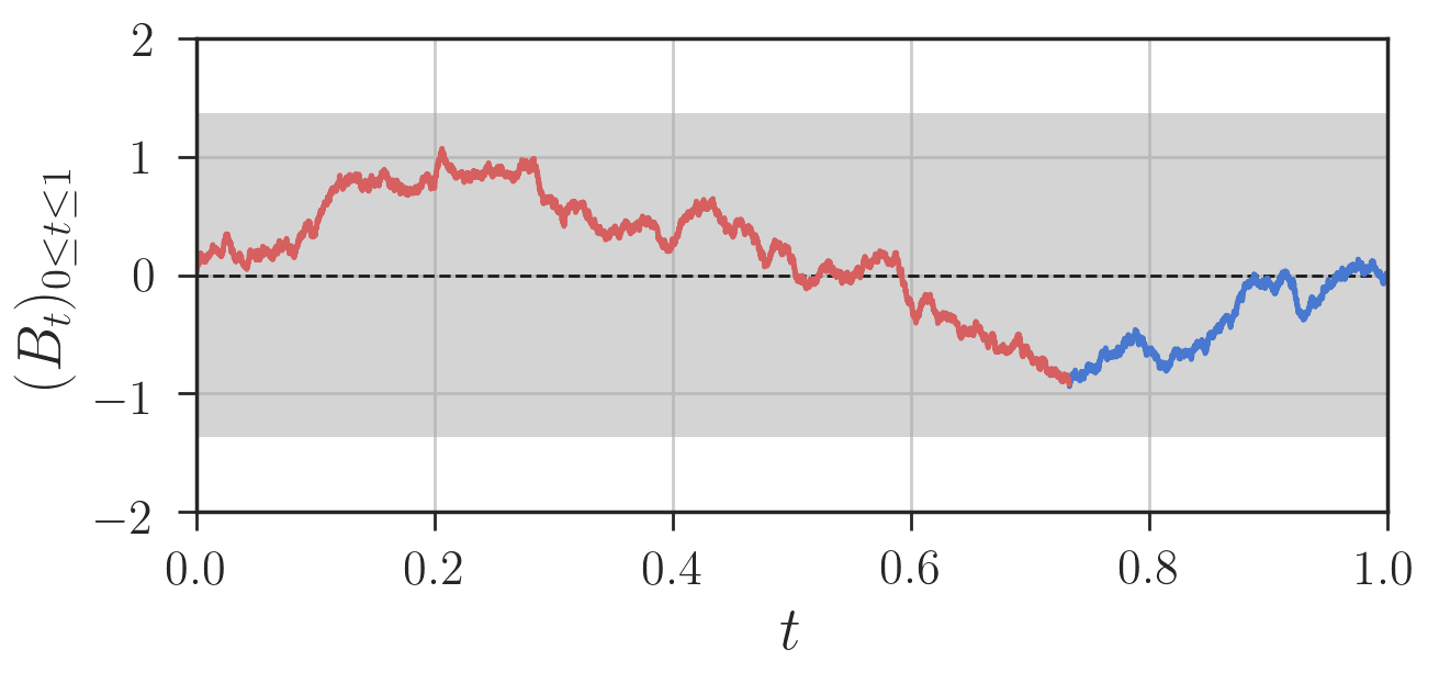
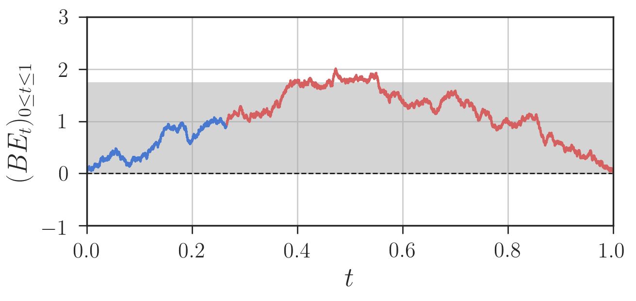
Figure 1: Example realizations of both the Brownian Bridge process (left) as well as the Brownian Excursion process, here constructed via circular shift of existing Brownian Bridge realization (right). Coloring indicates the re-arrangement used to construct the Brownian Excursion. For both processes, the 95% confidence region for the process is given in grey. In this case, a Brownian Bridge process well within the confidence interval ($\approx[-1.365,1.365]$) constructs a Brownian Excursion process whose maximum leaves the interval ($\approx[0,1.745]$).

The procedure we have just described is nothing more than finding the extremal value of a Brownian Excursion,

$$\underset{0\leq t\leq 1}{\max}BE_{t}=\underset{0\leq t\leq 1}{\max}B_{t}-\underset{0\leq t\leq 1}{\min}B_{t}.$$ (20)

The rejection zone can be computed according to

$$\mathbb{P}\left[\left\{\underset{0\leq t\leq 1}{\max}BE_{t}\right\}>\alpha\right]=2\sum_{i=1}^{\infty}(4i^{2}\alpha^{2}-1)e^{-2i^{2}\alpha^{2}}.$$ (21)

Process Normalization.

The overall maximum of a Brownian motion, or a Brownian bridge, are natural statistics to consider, however they treat the entire interval $[0,1]$ to be homogeneous. However, it is much more likely to observe the maximum value at the right extreme for Brownian motion, or the center for the Brownian bridge. Therefore, even if there is a signal in the zone of low variance, we compare it to the maximum over the entire interval and therefore it might easily be overlooked.

This problem can be solved by considering a rejection zone taking into account the changing variance of the underlying process. In the case of a Brownian motion, such normalization means that the rejection zone becomes a square root hull $t\alpha$, and in the case of a Brownian bridge, the hull shape is defined by $\sqrt{t(1-t)}$.

Area Tests.

Algorithm 1 Single Cumulative Test

Input:

$X$: Set of Patient Covariates

$T$: Treatment Indicators

$R$: Measured Outcome (endpoint)

$M$: Number of Monte-Carlo Simulations

Preprocessing

for $i\in 1,\dots,N$ do

     $R_{i}\leftarrow R_{i}-\mathbb{E}[R|T=T_{i}]$

     $T_{i}\leftarrow T_{i}-\mathbb{E}[T]$

     $Y_{i}\leftarrow R_{i}\cdot T_{i}$

$\mathcal{H}_{0}$ Statistics via MC

for $k\in 1,\dots,M$ do

     $\mathbf{q}$ $\leftarrow$ RandomPermute([1, 2, …, N])

     $C\leftarrow(\sum_{i=1}^{n}Y_{q_{i}})_{1\leq n\leq N}$

     $S[k]$ $\leftarrow$ Test statistics on $C$

Test on True Data

$\mathbf{s}\leftarrow{\rm SortPermutation}(X)$

$C\leftarrow(\sum_{i=1}^{n}Y_{s_{i}})_{1\leq n\leq N}$

$V$ $\leftarrow$ Test statistics on $C$

Output:

$p\text{-value}\leftarrow\frac{1}{M}\sum_{k=1}^{M}{\mathbf{1}_{S[k]>V}}$

Finally, we propose two more tests based on the total area under the curve (AUC) statistic, the idea behind the use of the entire area is that even if the maximum value does not reach the critical threshold, the fact that there are multiple points where the process approaches the limit may be indicative of a presence of a signal.

The test statistic in this case is computed as

$$A=\sum_{i\in[1,N]}\quad\left\lvert\frac{1}{\sqrt{N\sigma_{N}^{2}}}\cdot C_{i}^{j}\right\rvert.$$ (22)

We also consider a modification of this test where we sum squared values of the cumulative process,

$$SA=\sum_{i\in[1,N]}\quad\left(\frac{1}{\sqrt{N\sigma_{N}^{2}}}\cdot C_{i}^{j}\right)^{2}.$$ (23)

Implementation.

Depending on a prior knowledge about the type of the signal, other tests can be introduced as well. Since it is not always possible to have a closed form for the statistic distribution, we use a general numerical framework based on Monte-Carlo (MC) simulations to compute statistic critical values [22, 23]. We describe the process for this evaluation in Alg. 1.

4.3 Combined Test

As mentioned in the previous section, one may prefer different tests depending on the type of the signal one expects to observe in the data. However, it is not always possible, or desirable, to choose a particular test a priori. Instead, one might run all tests in parallel to see if some signal is detected by at least a single test. This procedure is a classical multiple test, and thus one needs to use a correction procedure for calculation of the final $p$-value in order to ensure that the Type-I error is not inflated. Standard correction procedures, such as Bonferoni correction [18], may be too severe, obfuscating the detection of significant covariates in practice. This is especially true in our case due to high correlation between our proposed significance tests, thus leading to a significant loss in combined test power. However, as in [24], it is possible to adapt our numeric procedure to run multiple tests simultaneously without any losses in Type-I or Type-II errors.

Test Name Description Baselines MoLin Modified outcome linear regression test Max Max of Brownian motion Proposed MaxB Max of Brownian bridge $\text{\it MaxB}_{N}$ Max of Brownian bridge, normalized via $\sqrt{t(1-t)}$ MaxBE Max of Brownian excursion $\text{\it MaxBE}_{N}$ Max of Brownian excursion normalized via $\sqrt{t(1-t)}$ AreaB Area under Brownian bridge SAreaB Squared area under Brownian bridge

Table 1: List of statistical tests for the identification of covariate-treatment interactions evaluated in this work.

Specifically, when calculating the combined significance test, for each covariate permutation of the centered treatment response, we compute the list of metrics defined by each statistical test included in the combined test, along with their corresponding $p$-values. Subsequently, we compare the vector of observed statistics with samples generated from random permutations of the centered treatment response. Then, of all the $p$-values for the individual tests in the combined test, we use the minimum $p$-value as the final aggregated statistic. From this minimum, we define the order on the set of vectors with $p$-values and also compute the $p$-value of the combined test. We present the pseudo-code for this combined test in Alg. 2.

In our experiments, we combine MaxB, MaxB_N, MaxBE, SAreaB, and SAreaB for our final combined significance test, thus accounting for many possible signal shapes. Selecting this subset, rather than applying all possible tests, reduces the computational burden of running the combined test. In practice, it is also possible to build a combined test tailored to a priori knowledge about a given dataset, as long as such a construction is fixed prior to any analysis of the dataset under investigation.

4

4.4 Multi-dose trials

Algorithm 2 Combined Test

Input:

$X$: Set of Patient Covariates

$T$: Treatment Indicators

$R$: Measured Outcome (endpoint)

$M$: Number of Monte-Carlo Simulations

$[F_{1},\dots,F_{L}]$: List of $L$ Tests to Combine

Preprocessing

for $i\in 1,\dots,N$ do

     $R_{i}\leftarrow R_{i}-\mathbb{E}[R|T=T_{i}]$

     $T_{i}\leftarrow T_{i}-\mathbb{E}[T]$

     $Y_{i}\leftarrow R_{i}\cdot T_{i}$

$\mathcal{H}_{0}$ Statistics via MC

for $m\in 1,\dots,M$ do

     $\mathbf{q}$ $\leftarrow$ RandomPermute([1, 2, …, N])

     $C\leftarrow(\sum_{i=1}^{n}Y_{q_{i}})_{1\leq n\leq N}$

     for $l\in 1,\dots,L$ do

         $S[l,m]$ $\leftarrow$ $F_{l}(C)$      

Distribution of Minimum $p$-value

for $k\in 1,\dots,M$ do

     $P[k]$ $\leftarrow$ $\underset{l}{\min}\quad\frac{1}{M}\sum_{m=1}^{M}{\mathbf{1}_{S[l,m]>S[l,k]}}$

Test on True Data

$\mathbf{s}\leftarrow{\rm SortPermutation}(X)$

$C\leftarrow(\sum_{i=1}^{n}Y_{s_{i}})_{\mathbf{1}\leq n\leq N}$

$V\leftarrow\underset{l}{\min}\quad\frac{1}{M}\sum_{m=1}^{M}{\mathbf{1}_{S[l,m]>F_{l}(C)}}$

Output:

Combined $p\text{-value}\leftarrow\frac{1}{M}\sum_{k=1}^{M}{\mathbf{1}_{P[k]>V}}$

Up to this point, we have considered the case of a clinical trial with only two treatment groups (e.g. placebo vs. treatment). However, in many cases, such as Phase II trials, multiple treatment doses are tested in parallel. In this section, we demonstrate how our approach may be generalized to the case of multiple doses trials. The generalization is quite straightforward: instead of $T\in\{\pm 1\}$ being a binary variable, we let instead $T\in\mathcal{T}\subset\mathbb{R}$ be a real-valued encoding of different doses. The set $\mathcal{T}$ may be a discrete scale encoding only dose order, or perhaps a more precise representation of the dosing amount, e.g. log value of the amount of administered treatment.

As in the binary case, the only important condition we need to ensure is that $\mathbb{E}[T]=0$. As long as this is true, then we can directly apply the modified outcome transformation and use the framework of cumulative processes without any additional modifications. In essence, in the binary case we focus on the conditional correlation between $R$ and a centered binary variable $T$ conditioned on $X$, and in the multi-dose case we do the same thing only with $T$ being simply centered.

5 Synthetic Experiments

In order to evaluate the efficiency of the proposed approach in an objective manner with known ground-truth, we generate a synthetic dataset of clinical trials. Although these models do not reflect the full complexity of such data in practice, we consider synthetic models for two main reasons: (i) to validate the ability of the evaluated statistical tests to accurately recover covariates which are known to be significantly correlated with the treatment, and (ii) to investigate particular cases of linear and non-linear interactions between covariates and treatment effects, demonstrating the strengths and weaknesses of each test. We list all of evaluated statistical tests in Table 1. Additionally, we demonstrate how to construct synthetic datasets for which each of the proposed test will fail, giving insight into the failure cases for each of the proposed statistical tests. We will also show that the combined test proposed in Sec. 4.3 provides near best-case accuracy for most of the tested synthetic models.

5.1 Synthetic models

For our experiments, we construct a wide array of synthetic treatment response curves whose purpose is to simulate the complex behavior observed in real-world clinical trials. Below, we describe each of the different synthetic models.

We consider three types of synthetic models, in order of increasing complexity, (i) a linear model, (ii) a set of piecewise-constant models, and (iii) a fully non-linear model.

For all these models, we generate covariates as i.i.d. uniform random variables over $[0,1]$. Next, given the full set of patient covariates $X$, we write the response model in the general form,

$$R[T|X] =W_{\rm trend}(X)+T\cdot W_{\rm interact}(X)+\epsilon,$$ (24)

where $\epsilon\sim\mathcal{N}(0,\Delta)$ is a noise term with variance $\Delta$, and $W_{\rm trend}(\cdot)$ and $W_{\rm interact}(\cdot)$ are functions operating across the set of covariates.

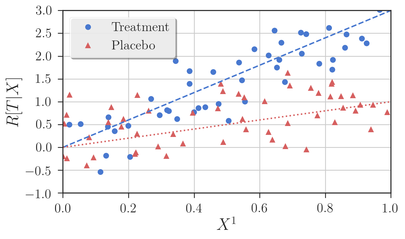
(a) L for $\Delta=0.25$, $W_{1}=2$, $W_{2}=1$

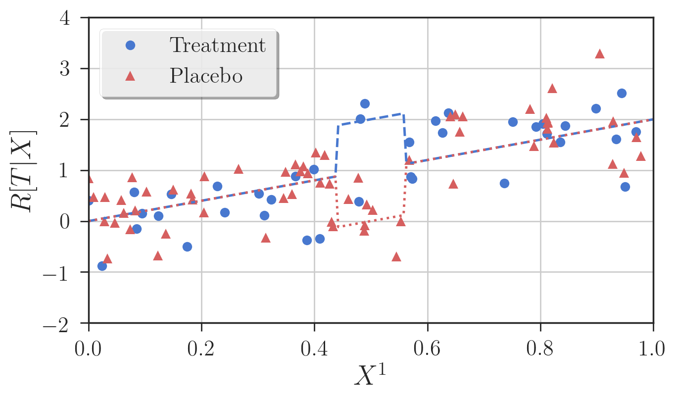
(b) PC-Int₂ for $\Delta=0.25$, $W_{1}=2$, $W_{2}=1$

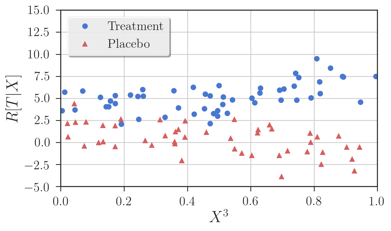
(c) NL for $\Delta=0.25$

Figure 2: Example $R[T|X]$ curves of different synthetic models for $N=100$.

Linear Model.

The linear model (L) corresponds to the case where $W_{\rm trend}$ and $W_{\rm interaction}$ are linear functions of the of the first covariate, in this case

$$W_{\rm trend}(X) =W_{1}X^{1},$$ (25)

$$W_{\rm interact}(X) =W_{2}X^{1}.$$ (26)

A successful test for L would report $X^{1}$ as a statistically significant covariate in terms of treatment interaction, and all other covariates would be rejected.

Piecewise-constant Models.

These proposed piecewise-constant (PC) synthetic models contain either one or two discontinuous jumps, denoted as thresholding and interval effects, respectively. Such discontinuities are not captured in linear models, however such effects are ubiquitous throughout biology and medicine.

We introduce four versions of PC models to capture these different configurations. All choices of $W_{\rm interaction}(X)$ are simple indicator functions with different supports to capture both thresholding and interval discontinuities. We present two thresholding models containing a single jump discontinuity, PC-Th₁ and PC-Th₂, as well as two interval models containing two jump discontinuities, PC-Int₁ and PC-Int₂,

$$W_{\rm interact}(X) =W_{2}\mathbf{1}_{[\nicefrac{{1}}{{2}},1]}(X^{1}),$$ (PC-Th₁)

$$W_{\rm interact}(X) =W_{2}\mathbf{1}_{[0,\nicefrac{{1}}{{8}}]}(X^{1}),$$ (PC-Th₂)

$$W_{\rm interact}(X) =W_{2}\mathbf{1}_{[\nicefrac{{1}}{{4}},\nicefrac{{3}}{{4}}]}(X^{1}),$$ (PC-Int₁)

$$W_{\rm interact}(X) =W_{2}\mathbf{1}_{[\nicefrac{{7}}{{16}},\nicefrac{{9}}{{16}}]}(X^{1}).$$ (PC-Int₂)

Finally, for each of the four different PC models, we use a linear baseline trend of $W_{\rm trend}(X)=W_{1}X^{1}$.

Non-linear model.

For the non-linear model (NL), we utilize the fourth synthetic scenario reported in Sec. 4 of [9]. Specifically, the covariate-treatment signal is generated according to

$$W_{\rm trend}(X) =1+2X^{1}+X^{2}+0.5X^{3},$$ (27)

$$W_{\rm interact}(X) =1-\left(X^{1}\right)^{3}+\exp\{\left(X^{3}\right)^{2}+X^{5}\}+0.6X^{6}-\left(X^{7}+X^{8}\right)^{2}.$$ (28)

We note that covariate $X^{4}$ is already a decoy covariate in this definition. Additionally, covariates $X^{7}$ and $X^{8}$ are symmetric.

Experimental Parameters.

For our experiments, we evaluated the proposed statistical tests on the given synthetic models over a range of easy and difficult settings. Overall,the difficulty of the task can be controlled by modifying $\Delta$, the ratio between baseline and treatment effect ($\nicefrac{{W_{1}}}{{W_{2}}}$), and the number of significant covariates versus total number of decoy covariates. Specifically, we construct our experiments along these three axes in the following manner.

• Noise: The variance of the noise term is evaluated over the range $\sqrt{\Delta}\in[1,8]$.

• W1: The ratio between the scale of the trend term (baseline coefficient) and the interaction term. Here, we fix $W_{2}=1$ while varying $W_{1}$ over $[1,5]$.

• Decoy: Given the fixed number of significant covariates, 1 for L and PC and 7 for NL, $D$ decoy covariates drawn i.i.d. randomly are added to the dataset. We vary $D$ over $[1,100]$.

Performance metrics.

Each of the evaluated significance tests are compared based on their statistical power when their Type-I errors are fixed. Specifically, after generating synthetic data several times and performing all with a $p$-value 0.05 significance threshold, we compare the significance tests by their ability to detect the known significant covariates in each synthetic model.

Since the test power is a function of many parameters describing various aspects of signal-to-noise ratio, in our experiments we also trace test sensitivity as a function of the experimental axes described in the previous section. We then compare the resulting curves to estimate which test provides the best performance over the tested range. Fig. 3 shows an example of such curves for different significance tests performed on the PC-Int₁ model under varying noise and baseline strength. As an aggregate measure for overall test performance, we compute the area under each curve. In this particular example, MaxBE is the best performing significance test, as it is capable of detecting the signal more often than alternative approaches.

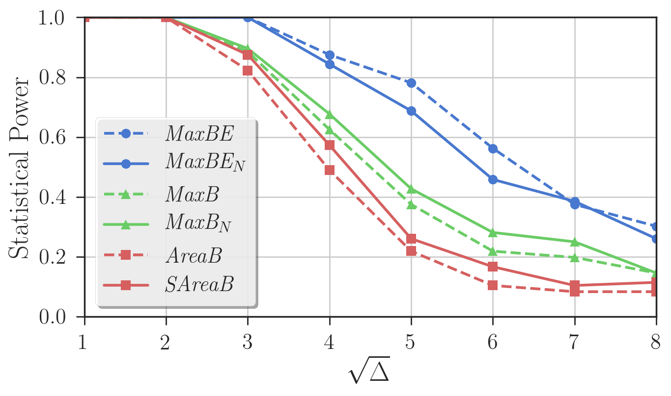
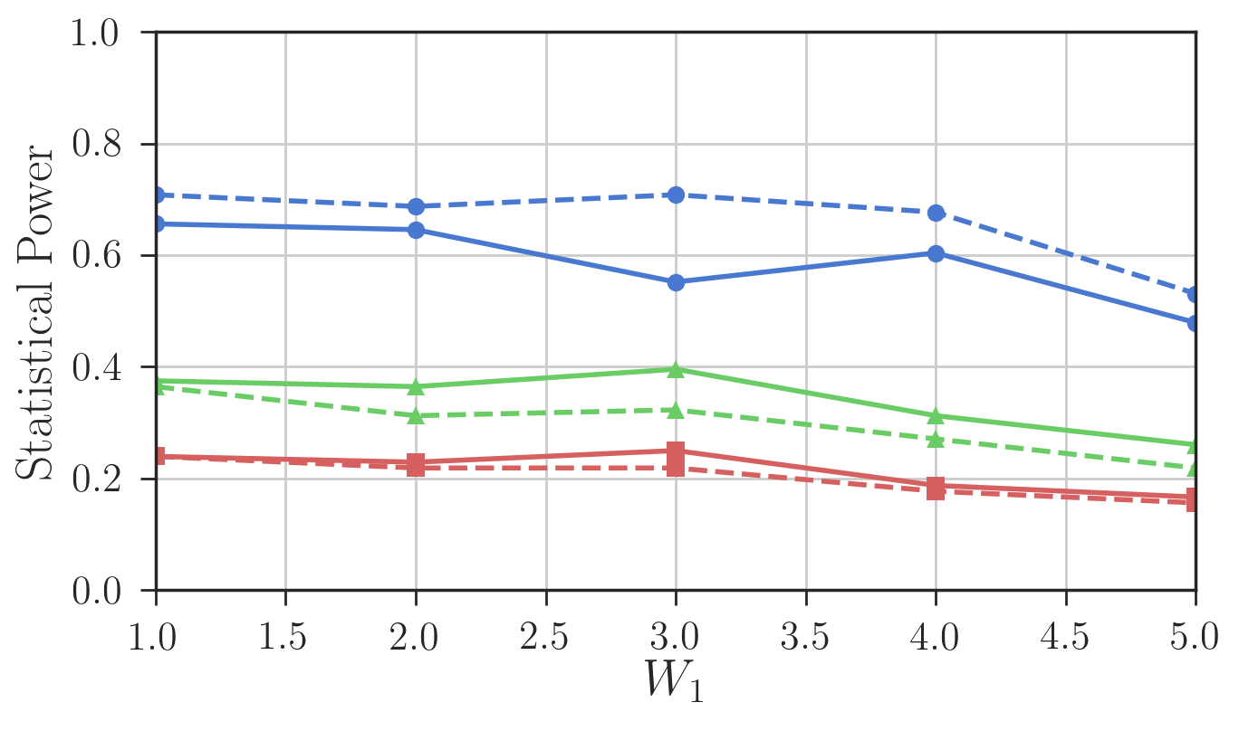
Figure 3: Comparison of individual tests for model PC-Int₁ under varying experimental parameters. Left Comparison over noise standard deviation, $\sqrt{\Delta}$. Right: Comparison over the value of the model baseline coefficient $W_{1}$. The legend remains consistent over both charts.

5.2 Results

Centering effect.

Fig. 4 shows the improvement made by removing the average values on each group of patients, comparing only the Max tests performed on either a Brownian-Motion-like process (no centering) or on a Brownian-Bridge-like process (centering). For visual convenience, the scores are normalized by the maximum value per dataset (column) such that there is alway a test with the performance score equal to 1 in each simulation scenario. As expected from our theoretical analysis, we observe that the test with centering correction (MaxB), in general, provides better significant covariate detection than the test with no centering correction (Max).

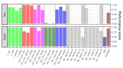
Figure 4: Detailed performance comparison between Brownian Motion (un-centered response) Max and Brownian Bridge (centered response) MaxB tests over the evaluated models and experimental parameters.

Main result summary.

A global summary of the main results is presented in Fig. 5 for the cumulative process tests MaxB, $\textit{MaxB}_{N}$, MaxBE, $\textit{MaxBE}_{N}$, AreaB, SAreaB, the baseline linear correlation test with modified outcome MoLin, and also for the combined test Comb. On this chart, each row corresponds to the designated test, while each column corresponds to a particular synthetic model and the varied parameter (noise, W1, or decoy), as described in Sec. 5.1.

The first set of columns corresponds to model L. We report that most of the tests have the same statistical power for the detection of the significant covariate $X^{1}$ for this model. As expected, the linear test MoLin performs very well, similarly to tests which are sensitive to a global measurements on the cumulative process, such as AreaB and SAreaB, since averaging over the whole curve provides more robustness. The MaxBE test does not perform well on linear data, as it is designed to capture transient correlations. Because of this feature, for L, it mostly detects unrelated fluctuations. The combined test Comb is also shown to perform very well in the linear setting.

The next four sets of columns correspond to the piecewise constant models (PC) and their associated experimental axes. For this class of models, the tests under study perform very differently, revealing the strengths of each individual test, which we now describe.

i) Threshold detection. As expected, MaxB performs the best for detection of threshold effects, at least when threshold is centrally located (PC-Th₁). Actually, this task appears relatively easy since most tests report good power, even MoLin. However, when the threshold is closer to the boundaries, and therefore more difficult to detect as in PC-Th₂, the MaxB test fails to recognize the significant covariate, as do most of the other tests. However, MaxBN performs very well in this setting due to the normalization hull which brings more power to the extreme sides of.

ii) Interval detection. This task appears to be very difficult for most tests, which fail catastrophically on both PC-Int₁ and PC-Int₂. The MaxB and $MaxB_{N}$ tests can only detect a single jump discontinuity, while AreaB, SAreaB, and MoLin are global measures which are unable to capture such a localized phenomenon. The only two tests which give strong positive results on this task is the MaxBE test and its normalized version $MaxBE_{N}$, since large excursions of the cumulative process correspond to a transient effect on the covariates.

We also see that Comb demonstrates very robust behavior across all the tested models and experimental parameters. While it does not always provide the best possible performance, its strength lies in its ability to operate in widely varied settings, from global linear trends to narrow threshold or interval effects.

Finally, to see how those tests would perform on less artificial models, the next set of columns correspond to experiments performed on the NL model. Here, we report the detection performance for each of the significant variables in NL. Once again, we observe that particular experimental configurations of this model can lead to individual test failures. However, once again we see that Comb demonstrates very robust performance across all tested experimental parameters.

These synthetic experiments have illustrated the ability of each individual test to detect known significant covariates under specific assumptions. When those assumptions are known a priori by the investigator (e.g. a known threshold effect), then it may be wiser to select the individual test according to this knowledge. However, when this knowledge is not available or too uncertain, our analysis suggests that Comb could be a robust solution. We present our full set of results both in terms of normalized AUC as well as raw statistical power in Appendix B.

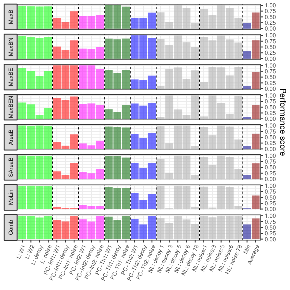
Figure 5: Visual representation of results obtained from all proposed statistical tests, along with the baseline MoLin, when performed over the synthetic treatment-interaction models (L, PC, and NL) described in Sec. 5. Evaluated significance tests are given as rows while synthetic models and the experimentation parameter are given as columns. Colors are used to indicate different synthetic models. Presented performance scores are given as the normalized area under the curve over the tested experimental parameter (noise, $W_{1}$, decoy). Normalization is performed over the significance tests such that the best-performing test reports a performance score of 1. The final two columns represent the aggregate minimum and average performance of each significance test over the set of tested models and experimentation parameters. Each significance is shown to perform well on some models but worse on others. Notably, the combined test (Comb, last row), shows robust performance across all experiments.

6 Exploration on Real Trials

We now turn our attention to the utility of our new individual tests and their combination in a more realistic setting. In this section, we describe results of application of our method to several real world clinical trial datasets. For these datasets, there are no known ground truths for significant covariates. However, as we control Type-I error, we can deduce that detecting more significant covariates is a desirable property for a successful statistical test on these real datasets.

6.1 CALGB 40603 (NCT00861705)

The primary objective of this study was to investigate whether adding bevacizumab to paclitaxel (+/- carboplatin) and subsequent dose-dense doxorubicin and cyclophosphamide (ddAC) significantly raises the rate of pathologic complete response (pCR) in the breast of patients with HR-poor/ HER2(-), resectable breast cancer [25]. The patient level data of this study can be retrieved from Project DataSphere [26]. The dataset contains the information on 443 patients randomly assigned to four different arms,

1. paclitaxel $\rightarrow$ ddAC,

2. paclitaxel + bevacizumab $\rightarrow$ ddAC + bevacizumab,

3. paclitaxel + carboplatin $\rightarrow$ ddAC,

4. paclitaxel + carboplatin + bevacizumab $\rightarrow$ ddAC + bevacizumab.

The dataset contains 45 covariates that can be used to explain the treatment effect when comparing the 4 arms.

Table 2 provides the number of significant variables (0.05 $p$-value significance threshold after Bonferoni correction) detected by the various tests when comparing Arm 1 versus 2, 1 versus 3, etc. For example, there two significant interactions when we compare Arms 2 and 4, the clinical N-stage (characterization of the regional lymph node involvement) and clinical T-stage (characterization of the size and extent of the tumor). We see that these covariates are detected only by the combined test, meaning that the application of individual test would not have been sufficient for the detection of this interaction. A similar phenomenon is observed when we analyze the results of the comparison of Arms 3 and 4. Two significant descriptors are detected: clinical N-stage and number of sentinel nodes examined. Again, only the combined test was capable of detecting both interactions simultaneously. Fig. 6 shows examples of the cumulative curves corresponding to significant variables for the comparison of Arms 3 and 4.

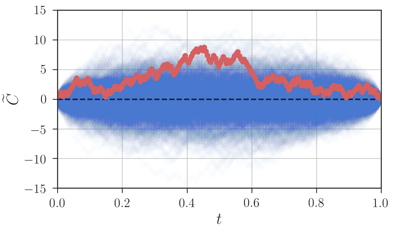
Figure 6: CALGB 40603 dataset, Arm 4 versus Arm 3. Cumulative processes generated from true covariate data (red) is contrasted with those constructed from random patient permutations (blue). Left: Evaluation of the clinical N-stage covariate. Right: Evaluation of the number of sentinal nodes examined covariate.

In both cases, the impact is negative, meaning that smaller covariate values correspond to larger differences between treatment and placebo (or reference treatment) arms, therefore implying that patients with smaller values of these covariates are more likely to benefit from the administration of bevacizumab. Since each of the detected covariates characterize the complexity of the tumor, the discovered dependencies suggest that patients at early stages of the disease are more likely to benefit from the addition of bevacizumab.

6.2 BCRP

The objective of this study was to compare the impact of nutritional and educational interventions on the psychological and physical adjustment after treatment for early-stage breast cancer [27]. The dataset was retrieved from the Quint package [28]. In total, there are 252 patients split into three arms: Arm 1: nutrition intervention ($N=85$), Arm 2: educational intervention ($N=83$), Arm 3: standard care ($N=84$). Similar to the CALGB results, as shown in Table 2, the combined test was the most sensitive test (0.05 $p$-value threshold after Bonferoni correction), indicating that the nationality covariate is a significant factor in determining the physical functioning score (SF36).

6.3 ACOSOG Z6051 (NCT00726622)

This is a randomized Phase-III trial evaluating the safety and efficacy of laparoscopic resection for rectal cancer [29]. The 462 patients were split into two groups: Arm 1 (open rectal resection) and Arm 2 (laparoscopic rectal resection). Among all tests, as shown in Table 2, the combined test and extermal of the normalized Brownian Bridge test were capable of detecting one covariate significantly correlated with the efficacy of the treatment regime (0.05 $p$-value significance threshold after Bonferoni correction): distance to nearest radial margin. The cumulative process corresponding to this variable is shown in Fig. 7, where patients with lower values of the distance to nearest radial margin covariate are shown to be more likely to benefit more from the laparoscopic rectal resection. The distance to nearest radial margin variable is not a parameter that can be assessed prior to the intervention, it is a characteristic that can be measured once the operation is complete. Therefore, it can not be used to guide the selection of the intervention type. However, such post-treatment dependencies can provide useful insights into the circumstances where a treatment of interest may prove most efficient.

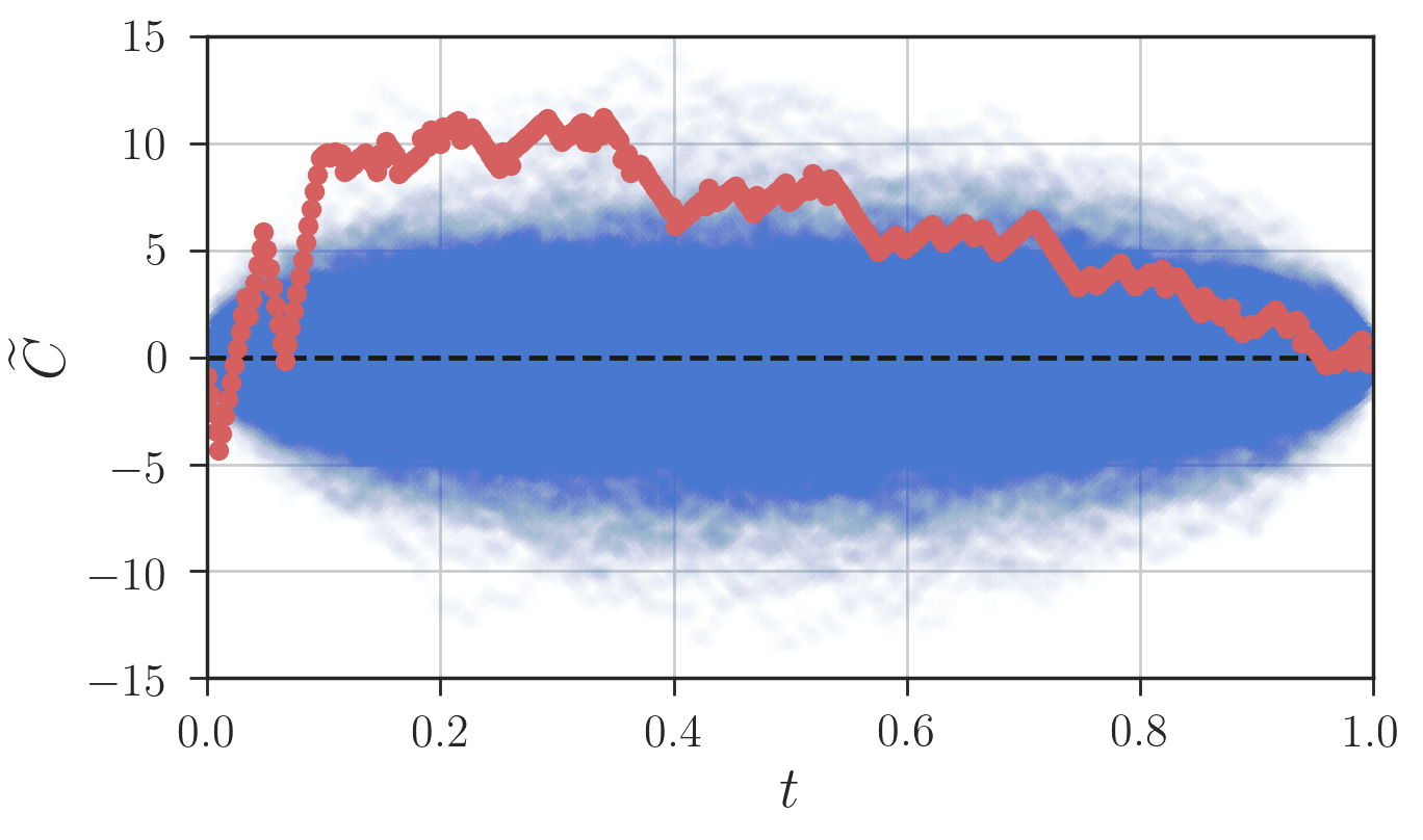
Figure 7: ACOSOG Z6051 dataset evaluated for the distance to nearest radial margin covariate. Cumulative processes generated from true covariate data (red) is contrasted with those constructed from random patient permutations (blue).

CALGB BCRP (C) BCRP (P) ACOSOG Test 1v2 1v3 1v4 2v4 3v4 1v3 2v3 1v3 2v3 1v2 Total MoLin 0 0 0 0 0 0 0 0 0 0 0 Max 0 0 0 0 0 0 0 0 0 0 1 $\textit{MaxB}_{N}$ 1 0 1 0 1 0 0 0 0 1 4 MaxBE 0 0 0 0 0 0 0 0 0 0 0 AreaB 0 0 0 0 1 0 0 0 0 0 1 SAreaB 0 0 0 0 1 0 0 0 0 0 1 Comb 1 0 2 2 2 0 0 0 1 1 9

Table 2: Number of significant features detected by various statistical tests in CALGB 40603, BCRP and ACOSOG Z6051 studies. BCRP (C) and (P) correspond to two different endpoints defined in the study: CESD score and SF36 scores. Each row corresponds to a particular test. See Table 1 for test name abbreviations. Columns names “AvB” describe comparisons between different arms of the study; see text for a more detail descriptions of study arms. The last column (Total) reports the total number of significant variables detected by each test across all evaluated studies.

7 Discussion

In this paper, we presented a series of new statistical tests tailored for the detection of complex, non-linear treatment-covariate dependencies in clinical trial datasets. We describe how to merge these tests into a single combined test capable of efficiently detecting different types of interactions. We illustrated the performance of the proposed approach on various synthetic models, where we compare it to existing approaches. We also describe an application of the proposed procedure to three real world clinical trial datasets where we observed that our proposed tests do indeed allow one to detect signals which can go undiscovered using existing approaches.

The proposed technique is a univariate procedure tailored for the detection of single biomarkers, and therefore is relatively easy to interpret with respect to multivariate approaches. However, this characteristics is also a significant limitation of the procedure since, as with any univariate approach, one needs to apply multiple testing correction (e.g. Bonferoni) to account for the number of covariates analyzed. In some cases, this correction might be too drastic. This issue can be partially resolved by imposing a pre-order on the list of covariates defined by an expert or by automatically extracting an ordering from the literature or an external dataset. Another consequence of the nature of univariate tests is that such a test can miss complex dependencies involving multiple covariates if each of them separately do not present statistically significant signals.

In our future research, we plan generalize our proposed cumulative tests to a multivariate setting, and explore the possibility of building a statistical test capable of detecting non-linear multivariate dependencies with a proper control over Type-I error. Another interesting direction is the incorporation of external data sources as prior knowledge. By continuing to analyze publicly available clinical trial datasets, we hope to find new and interesting covariate dependencies, as well as to construct a large benchmark of datasets for the comparison of covariate-detection methods.

In this article, we focused on the detection of covariates interacting with the treatment efficacy. Such covariates provide a natural basis for sub-group selection. The extension of the proposed statistical tests for sub-group identification is another important direction that we hope to address in our future work.

Appendix A Outcome Centering Proofs

A.1 Proof of Lemma 1

As stated in the lemma, we assume that a “general” modified outcome written in the form $\widehat{Y}=T\cdot(R+f(T))$, where $f(T)$ is an arbitrary function of $T$. Looking at the variance of this general modified outcome we have

$$\mathbf{var}[\widehat{Y}]=\mathbf{var}\left[T\cdot(R+f(T))\right].$$ (29)

Using the law of total variation, we next condition on the treatment, $T$,

$$\mathbf{var}[\widehat{Y}]= \mathbb{E}\left[\mathbf{var}_{R}\left[T\cdot(R+f(T))|T\right]\right]$$

$$+\mathbf{var}\left[\mathbb{E}_{R}\left[T\cdot(R+f(T))|T\right]\right].$$ (30)

The conditional variance can be written as

$$\mathbf{var}_{R}\left[T\cdot(R+f(T))|T\right] =T^{2}\cdot\mathbf{var}\left[R|T\right],$$ (31)

which follows from the application of the translational invariance property as well as the scaling identity. Subsequently, for the conditional expectation, we find

$$\mathbb{E}_{R} \left[T\cdot(R+f(T))|T\right]$$

$$=\mathbb{E}_{R}\left[T\cdot R|T\right]+\mathbb{E}_{R}\left[T\cdot f(T)|T\right]$$

$$=T\cdot(\mathbb{E}\left[R|T\right]+f(T)),$$ (32)

which follows from both the linearity of expectation as well as the independence of $T$ from $R$. Taken together, we have

$$\mathbf{var}[\widehat{Y}] =\mathbb{E}\left[T^{2}\cdot\mathbf{var}[R|T]\right]$$

$$\quad+\mathbf{var}[T\cdot(\mathbb{E}[R|T]+f(T))].$$ (33)

From the above, we see that the only a variance term is dependent upon the choice of $f(T)$. Since the variance must not be negative, the minimum variance $\sigma^{*}=\mathbb{E}[T^{2}\cdot\mathbf{var}[R|T]]$ is obtained when $\mathbf{var}\left[T\cdot(\mathbb{E}[R|T]+f(T))\right]=0$. It can be directly observed that $f(T)=-\mathbb{E}[R|T]$ is one such choice of $f(T)$ for which $\mathbf{var}[\widehat{Y}]=\sigma^{*}$. ∎

A.2 Proof of Lemma 2

We first calculate the variance of the modified outcome as presented in [8]. Recalling $Y_{\rm mod}=T\cdot R$, we see

$$\mathbf{var} [Y_{\rm mod}]=\mathbf{var}[R\cdot T],$$

$$=\mathbb{E}[\mathbf{var}_{R}[T\cdot R|T]]+\mathbf{var}[\mathbb{E}_{R}[T\cdot R|T]],$$

$$=\mathbb{E}[T^{2}\cdot\mathbf{var}[R|T]]+\mathbf{var}[T\cdot\mathbb{E}[R|T]].$$ (34)

which follows first from the law of total variation, and also from our earlier calculations in Appendix A.1.

We now make the calculation of this variance explicit through the empirical per-trial first and second moments, $\mu_{T}$ and $\sigma_{T}^{2}$, respectively. For the first term,

$$\mathbb{E}[T^{2}\cdot\mathbf{var} [R|T]]$$

$$=\sum_{t\in\{\pm 1\}}\pi_{t}\cdot t^{2}\cdot\mathbf{var}[R|T=t],$$

$$=\frac{1}{2}\cdot(\sigma_{1}^{2}+\sigma_{-1}^{2})^{2}.$$ (35)

Subsequently,

$$\mathbf{var} [T\cdot\mathbb{E}[R|T]]$$

$$=\mathbb{E}[(T\cdot\mathbb{E}[R|T])^{2}]-\mathbb{E}^{2}[T\cdot\mathbb{E}[R|T]],$$

$$=\sum_{t\in\{\pm 1\}}\pi_{t}\cdot t^{2}\cdot\mathbb{E}^{2}[R|T=t]$$

$$\quad\quad-\left(\sum_{t\in\{\pm 1\}}\pi_{t}\cdot t\cdot\mathbb{E}[R|T=t]\right)^{2},$$

$$=\frac{1}{4}(\mu_{1}-\mu_{-1})^{2}.$$ (36)

Finally, we have

$$\mathbf{var}[Y_{\rm mod}]=\frac{1}{2}(\sigma_{1}^{2}+\sigma_{-1}^{2})+\frac{1}{4}(\mu_{1}-\mu_{-1})^{2}.$$ (37)

In contrast, we have the value of the modified outcome with per-treatment centering, as shown in Lemma 1,

$$\mathbf{var}[\widetilde{Y}] =\mathbb{E}[T^{2}\cdot\mathbf{var}[R|T]],$$

$$=\frac{1}{2}(\sigma_{1}^{2}+\sigma_{-1}^{2}).$$ (38)

Thus, for the ratio $\gamma=\frac{\mathbf{var}[\widetilde{Y}]}{\mathbf{var}[Y_{\rm mod}]}$,

$$\gamma =\frac{\frac{1}{2}(\sigma_{1}^{2}+\sigma_{-1}^{2})}{\frac{1}{2}(\sigma_{1}^{2}+\sigma_{-1}^{2})+\frac{1}{4}(\mu_{1}-\mu_{-1})^{2}},$$

$$=\frac{1}{1+\frac{1}{2}\cdot\frac{(\mu_{1}-\mu_{-1})^{2}}{\sigma_{1}^{2}+\sigma^{2}_{-1}}},$$

$$=1-{\rm sig}\left[\log\frac{(\mu_{1}-\mu_{-1})^{2}}{\sigma_{1}^{2}+\sigma_{-1}^{2}}-\log 2\right].$$ (39)

where ${\rm sig}(x)=\frac{1}{1+e^{-x}}$ is the logistic sigmoid function. Since ${\rm sig}(x)$ is bounded in range $[0,1]$ over the domain $x\in\mathbb{R}$, we can see that $\gamma\in[0,1]$, as well. Additionally, we see directly that the only instance in which $\gamma=1$ is the case that $\mu_{1}=\mu_{-1}$, that is, when the measured responses for both treatments have the same expectation. ∎

A.3 Proof of Lemma 3

The conditional covariance of the centered outcome can be shown to be

$$\mathbf{cov} [\widetilde{R},T|X]$$

$$=\mathbf{cov}\left[R-\mathbb{E}[R|T],T|X\right],$$

$$=\mathbf{cov}[R,T|X]-\mathbf{cov}[\mathbb{E}[R|T],T|X],$$

$$=\mathbf{cov}[R,T|X]-\mathbb{E}[T\cdot\mathbb{E}[R|T]|X],$$

$$\quad+\mathbb{E}[\mathbb{E}[R|T]|X]\cdot\mathbb{E}[T|X].$$ (40)

Assuming a properly randomized trial such that $T\perp X$ and centered treatment variables, $\mathbb{E}[T]=0$, then the covariance becomes

$$\mathbf{cov} [\widetilde{R},T|X]$$

$$=\mathbf{cov}[R,T|X]-\mathbb{E}[T\cdot\mathbb{E}[R|T]|X].$$ (41)

However, since $T\perp X$ and the measured outcome $R$ is a fixed property of the dataset which does not change based on the covariate selection $X$, we note that $\mathbb{E}[T\cdot\mathbb{E}[R|T]|X]=\mathbb{E}[T\cdot\mathbb{E}[R|T]]$. Thus, the second term is constant with respect to the covariate under test and we write it as $\mathcal{C}_{R,T}$. ∎

A.4 Proof of Lemma 4

The unconditioned covariance between the centered treatment response and the treatment indicators is

cov $$[\widetilde{R},T]$$

$$=\textbf{cov}[R-\mathbb{E}[R|T],T],$$

$$=\textbf{cov}[R,T]-\mathbf{cov}[\mathbb{E}[R|T],T],$$ (42)

which follows from the simple distributional property of the covariance. Since we assume centered treatment indicator variables, $\mathbb{E}[T]=0$, this difference in covariances can be simplified to the difference,

$$\textbf{cov}[\widetilde{R},T]=\mathbb{E}[T\cdot R]-\mathbb{E}[T\cdot\mathbb{E}[R|T]].$$ (43)

However, we can see that these two terms are equivalent. Using the total expectation, we observe that $\mathbb{E}[T\cdot R]=\mathbb{E}_{T}[\mathbb{E}_{R}[T\cdot R|T]]$, where we use subscripts to make the expectations explicit. Moving the constant $T$ outside of the conditional expectation, we have $\mathbb{E}[T\cdot R]=\mathbb{E}[T\cdot\mathbb{E}[R|T]]$, which shows the equivalence of the two terms. Thus, $\textbf{cov}[\widetilde{R},T]=0$. ∎

Appendix B Full Synthetic Results

References

- [1] D. W. Thomas, J. Burns, J. Audette, A. Carroll, C. Dow-Hygelund, and M. Hay, “Clinical development success rates 2006-2015,” BIO Industry Analysis, Biomedtracker, 2016.
- [2] R. K. Harrison, “Phase II and phase III failures: 2013-2015,” Nautre Reviews: Drug Discovery, vol. 15, pp. 817–818, 2016.
- [3] U. Food and D. Administration, “FDA grants accelerated approval to pembrolizumab for first tissue/site agnostic indication,” https://www.fda.gov/Drugs/InformationOnDrugs/ApprovedDrugs/ucm560040.htm, 2017, U.S. FDA Press Release, May 2017.
- [4] S. J. Pocock, S. F. Assmann, L. E. Enos, and L. E. Kasten, “Subgroup analysis, covariate adjustment and baseline comparisons in clinical reporting: current practice and problems,” Statistics in Medicine, vol. 21, no. 19, pp. 2917–2930, 2002.
- [5] M. Halperin, J. H. Ware, D. P. Byar, N. Mantel, C. C. Brown, J. Koziol, M. Gail, and S. B. Green, “Testing for interaction in an contingency table,” Biometrika, vol. 64, no. 2, pp. 271–275, 1977.
- [6] R. Simon, “Patient subsets and variation in therapeutic efficacy,” vol. 14, no. 4, pp. 473–482, 1982.
- [7] R. Wang, S. W. Lagakos, J. H. Ware, D. J. Hunter, and J. M. Drazen, “Statistics in medicine—reporting of subgroup analyses in clinical trials,” New England Journal of Medicine, vol. 357, no. 21, pp. 2189–2194, 2007.
- [8] L. Tian, A. A. Alizadeh, A. J. Gentles, and R. Tibshirani, “A simple method for estimating interactions between a treatment and a large number of covariates,” Journal of the American Statistical Association, vol. 109, no. 508, pp. 1517–1532, 2014.
- [9] Y. Zhao, D. Zeng, A. J. Rush, and M. R. Kosorok, “Estimating individualized treatment rules using outcome weighted learning,” Journal of the American Statistical Association, vol. 107, no. 449, pp. 1106–1118, 2012.
- [10] J. A. Koziol and S.-C. H. Wu, “Changepoint statistics for assessing a treatment-covariate interaction,” Biometrics, vol. 52, no. 3, pp. 1147–1152, 1996.
- [11] I. Lipkovich and A. D. R. B. D. Sr., “Tutorial in biostatistics: data-driven subgroup identification and analysis in clinical trials,” Statistics in Medicine, vol. 36, no. 1, pp. 136–196, 2017.
- [12] L. Tian and R. Tibshirani, “Adaptive index models for marker-based risk stratification,” Biostatistics, vol. 12, no. 1, pp. 68–86, 01 2011. [Online]. Available: http://www.ncbi.nlm.nih.gov/pmc/articles/PMC3006126/
- [13] A. Zeileis, T. Hothorn, and K. Hornik, “Model-based recursive partitioning,” Journal of Computational and Graphical Statistics, vol. 17, no. 2, pp. 492–514, 2008.
- [14] I. Lipkovich, A. Dmitrienko, J. Denne, and G. Enas, “Subgroup identification based on differential effect search—a recursive partitioning method for establishing response to treatment in patient subpopulations,” Statistics in medicine, vol. 30, no. 21, pp. 2601–2621, 2011.
- [15] J. C. Foster, J. M. Taylor, and S. J. Ruberg, “Subgroup identification from randomized clinical trial data,” Statistics in Medicine, vol. 30, no. 24, pp. 2867–2880, 2011.
- [16] E. Dusseldorp, C. Conversano, and B. J. Van Os, “Combining an additive and tree-based regression model simultaneously: STIMA,” Journal of Computational and Graphical Statistics, vol. 19, no. 3, pp. 514–530, 2010.
- [17] E. Dusseldorp and I. Van Mechelen, “Qualitative interaction trees: a tool to identify qualitative treatment–subgroup interactions,” Statistics in Medicine, vol. 33, no. 2, pp. 219–237, 2014. [Online]. Available: http://dx.doi.org/10.1002/sim.5933
- [18] O. J. Dunn, “Multiple comparisons among means,” Jounrnal of the American Statistical Association, vol. 56, no. 293, pp. 52–64, 1961.
- [19] M. D. Donsker, “An invariance principle for certain probability limit theorems,” Memoirs of the American Mathematical Society, no. 6, 1951.
- [20] J.-M. Azaïs and L.-V. Lozada-Chang, “A toolbox on the distribution of the maximum of gaussian process,” 2013.
- [21] A. N. Borodin and P. Salminen, Handbook of Brownian Motion—Facts and Formulae. Springer Basel, 2002.
- [22] J. Shao and D. Tu, The jackknife and bootstrap. Springer Science & Business Media, 2012.
- [23] J. J. Higgins, Introduction to modern nonparametric statistics. Cengage Learning, 2003.
- [24] J. Gates, “Exact Monte Carlo tests using several statistics,” Journal of Statistical Computation and Simulation, vol. 38, no. 1-4, pp. 211–218, 1991.
- [25] V. G. Abramson and I. A. Mayer, “Molecular heterogeneity of triple-negative breast cancer,” Current Breast Cancer Reports, vol. 6, no. 3, pp. 154–158, 2014.
- [26] A. K. Green, K. E. Reeder-Hayes, R. W. Corty, E. Basch, M. I. Milowsky, S. B. Dusetzina, A. V. Bennett, and W. A. Wood, “The project data sphere initiative: accelerating cancer research by sharing data,” The Oncologist, vol. 20, no. 5, pp. 464–e20, 2015.
- [27] M. F. Scheier, V. S. Helgeson, R. Schulz, S. Colvin, S. L. Berga, J. Knapp, and K. Gerszten, “Moderators of interventions designed to enhance physical and psychological functioning among younger women with early-stage breast cancer,” Journal of Clinical Oncology, vol. 25, no. 36, pp. 5710–5714, 2007.
- [28] E. Dusseldorp, L. Doove, and I. Van Mechelen, “Quint: An R package for the identification of subgroups of clients who differ in which treatment alternative is best for them,” Behavior Research Methods, vol. 48, no. 2, pp. 650–663, 2016.
- [29] J. Fleshman, M. Branda, D. J. Sargent, A. M. Boller, V. George, M. Abbas, W. R. Peters, D. Maun, G. Chang, and A. Herline, “Effect of laparoscopic-assisted resection vs open resection of stage II or III rectal cancer on pathologic outcomes: the ACOSOG Z6051 randomized clinical trial,” Journal of the American Medical Association, vol. 314, no. 13, pp. 1346–1355, 2015.