Inelastic Surface Growth

Abstract

Inelastic surface growth associated with continuous creation of incompatibility on the boundary of an evolving body is behind a variety of natural and technological processes, including embryonic development and 3D printing. In this paper we extend the recently proposed stress-space-centered theory of surface growth (PRL 119, 048001, 2017) by shifting the focus towards growth induced strains. To illustrate the new development we present several analytically tractable examples.

The paper is dedicated to the memory of Gérard Maugin, a scientific visionary.

I Introduction

In the process of surface growth the configuration of a body is changing as a result of continuous deposition of new matter on its boundary Skalak ; DiCarlo ; MauginCiarletta ; Goriely17 ; Tomassetti . Despite the ubiquity of such processes in both living and inert systems, the mechanical theory of surface growth, accounting for the development of inelastic strains in the growing body, is still far from being complete. This is rather remarkable given that the mechanical theory of volumetric growth, assuming that mass supply takes place in the bulk of the body, is well advanced MauginEpstein ; MauginCFG ; Yavari ; Kuhl ; BenAmar ; Ateshian ; Ambrosi ; ChapmanJones .

The approach to inelastic surface growth developed in the present paper is focused on the elastic incompatibility created at the instant of deposition. The associated inelastic strain is not evolving after accretion and therefore depends exclusively on the deposition protocol. Recently, relying on some previous insights Goodman ; Fletcher ; Trincher ; Naumov ; Arutyunyan ; Gambarotta ; SozioYavari ; Papadopoulos , we were able to link explicitly the deposition strategy with the final incompatibility ZT17 . However, the proposed description was limited to the stress space, which was possible because the growing surface was assumed to be loaded in a soft device.

To handle the case of a hard device, one needs to address the kinematical issues that were bypassed in the stress-centered formulation. This is the goal of the present paper where we introduce the instantaneous displacement field for the particles materializing on the growing surface, allowing us to separate elastic and inelastic strains. We distinguish further between compatible and incompatible inelastic strains and we link the latter to the accumulation of residual stresses.

As an illustration, we consider a bar growing by one of its ends. To see the development of incompatibility in this minimal setting we laterally constrain the bar by attaching it to an elastic background. We show that even in this elementary case the obtained solutions depend nontrivially on deposition protocols, suggesting interesting applications for reinforced masonry and additive manufacturing.

Throughout the paper we assume that strains are small and that dynamical effects can be neglected. A more general theory will be presented elsewhere.

II General theory

Kinematics. In order to track the evolution of material points after accretion, we introduce a reference mass reservoir $\mathscr{B}_{t}=\left\{\textbf{\emph{x}}\,|\,\vartheta(\textbf{\emph{x}})\leq t\right\}$. For simplicity, in this study the scalar function $\vartheta$ will be prescribed, even though in many realistic growth processes its evolution would have to be found self-consistently. The Lagrangian velocity of $\partial\mathscr{B}_{t}$ is then $D_{0}=(\nabla\vartheta(\textbf{\emph{x}})\cdot\textbf{\emph{n}}_{0}(\textbf{\emph{x}}))^{-1}$ where $\textbf{\emph{n}}_{0}=\nabla\vartheta(\textbf{\emph{x}})/|\nabla\vartheta(\textbf{\emph{x}})|$ is the reference outward normal. We can decompose $\partial\mathscr{B}_{t}=\Omega_{t}\cup\Omega_{d}$, where the time dependent growing part $\Omega_{t}$ is such that $D_{0}\neq 0$ while the time independent non-growing part $\Omega_{d}$ has $D_{0}=0$. Writing the incremental advance of the material surface $\Omega_{t}$ as $\Delta\textbf{\emph{x}}=D_{0}\textbf{\emph{n}}_{0}\Delta t$, where $\Delta t$ is an infinitesimal time interval, we obtain $j_{0}=\rho_{0}D_{0}$, where $j_{0}$ is the mass flux per reference surface and $\rho_{0}(\textbf{\emph{x}})$ is the time-independent volumetric mass density in $\mathscr{B}_{t}$. Since the reference configuration is defined only for the material points already in $\mathscr{B}_{t}$, it can be always chosen to coincide with the instantaneous actual placement of the body in $\textbf{R}^{3}$.

For each instant $t\geq\vartheta(\textbf{\emph{x}})$, we can introduce displacement of the attached material particles $\textbf{\emph{u}}(\textbf{\emph{x}},t)$. In particular, the instantaneous (initial) displacement at the moment of deposition is $\mathring{\textbf{\emph{u}}}(\textbf{\emph{x}})=\textbf{\emph{u}}(\textbf{\emph{x}},\vartheta(\textbf{\emph{x}})).$ The presence of this displacement field makes the Eulerian normal velocity $D$ of the accreting surface in the actual space $\omega_{t}$ different from the Lagrangian velocity $D_{0}$. More specifically, we can write $D=D_{0}+D_{0}(\nabla\mathring{\textbf{\emph{u}}})\textbf{\emph{n}}_{0}\cdot\textbf{\emph{n}}$, where n is the normal to $\omega_{t}$.

The difference between $D$ and $D_{0}$ plays a fundamental role in surface growth. For instance, in the process of 3D printing, the velocity of the printing head can be controlled independently of the mass flux. Since in this paper we neglect geometrical nonlinearities, we can assume that $\textbf{\emph{n}}_{0}\sim\textbf{\emph{n}}$ and write the relation between $D_{0}$ and $D$ in the form $D/D_{0}-1=(\nabla\mathring{\textbf{\emph{u}}})\textbf{\emph{n}}\cdot\textbf{\emph{n}}.$

Elastic growth. Assume that the reference configuration $\mathscr{B}_{t}$ is a stress free state for the growing body. If body forces b and surface tractions s are controlled during growth, equilibrium of intermediate configurations requires that, for all $t\in(0,T)$, where $T$ corresponds to the end of accretion,

$$\left\{\begin{array}[]{lcc}\text{div}\boldsymbol{\sigma}(\textbf{\emph{x}},t)+\textbf{\emph{b}}(\textbf{\emph{x}})=\textbf{\emph{0}}&\text{in}&\mathscr{B}_{t}\\ \boldsymbol{\sigma}(\textbf{\emph{x}},t)=\mathbb{C}(\textbf{\emph{x}})\nabla_{s}\textbf{\emph{u}}(\textbf{\emph{x}},t)&\text{in}&\mathscr{B}_{t}\\ \boldsymbol{\sigma}(\textbf{\emph{x}},t)\textbf{\emph{n}}(\textbf{\emph{x}})=\textbf{\emph{s}}(\textbf{\emph{x}})&\text{on}&\Omega_{t}\\ \textbf{\emph{u}}(\textbf{\emph{x}},t)=\textbf{\emph{0}}&\text{on}&\Omega_{d}\end{array}\right.$$ (1)

where $\boldsymbol{\sigma}(\textbf{\emph{x}},t)$ is the (symmetric) Cauchy stress tensor, $\mathbb{C}$ is a positive definite and symmetric elasticity tensor and $\nabla_{s}=(\nabla+\nabla^{\textsf{T}})/2$. Here we have assumed that the material behavior of the body is linearly elastic and that the strains are fully defined by the gradient of the displacement field $\textbf{\emph{u}}(\textbf{\emph{x}},t)$.

For each $t\in(0,T)$ the problem (1) admits a unique solution. In anticipation of what follows, we note that one can use (1) to obtain the “deposition protocol” represented, for instance, by the combination of boundary displacements and surface stresses on $\Omega_{t}$,

$$\left\{\begin{array}[]{lcc}\mathring{\textbf{\emph{u}}}(\textbf{\emph{x}})=\textbf{\emph{u}}(\textbf{\emph{x}},\vartheta(\textbf{\emph{x}}))\\ \mathring{\boldsymbol{\sigma}}_{a}(\textbf{\emph{x}})=\mathbb{P}(\textbf{\emph{x}})\boldsymbol{\sigma}(\textbf{\emph{x}},\vartheta(\textbf{\emph{x}}))\mathbb{P}(\textbf{\emph{x}})\end{array}\right.\quad\textbf{\emph{x}}\in\Omega_{t}$$ (2)

where $\mathbb{P}=\textbf{I}-\textbf{\emph{n}}\otimes\textbf{\emph{n}}$ is the surface projector. From (2) one can also compute the current velocity $D$, which in general will be different from $D_{0}$.

Inelastic growth. To allow for inelastic growth we modify the equilibrium problem as follows

$$\left\{\begin{array}[]{lcc}\text{div}\boldsymbol{\sigma}(\textbf{\emph{x}},t)+\textbf{\emph{b}}(\textbf{\emph{x}})=\textbf{\emph{0}}&\text{in}&\mathscr{B}_{t}\\ \boldsymbol{\sigma}(\textbf{\emph{x}},t)=\mathbb{C}(\textbf{\emph{x}})\left(\nabla_{s}\textbf{\emph{u}}(\textbf{\emph{x}},t)-\boldsymbol{\epsilon}_{p}(\textbf{\emph{x}})\right)&\text{in}&\mathscr{B}_{t}\\ \boldsymbol{\sigma}(\textbf{\emph{x}},t)\textbf{\emph{n}}(\textbf{\emph{x}})=\textbf{\emph{s}}(\textbf{\emph{x}})&\text{on}&\Omega_{t}\\ \textbf{\emph{u}}(\textbf{\emph{x}},t)=\textbf{\emph{0}}&\text{on}&\Omega_{d}.\end{array}\right.$$ (3)

Here we still assume that the elastic response of the body is Hookean, but we introduce the inelastic strain $\boldsymbol{\epsilon}_{p}(\textbf{\emph{x}})$. As it was first observed in a biological setting Nikitin , the inelastic strain defines a relaxed (stress-free) configuration which may not be isometrically embeddable into $\textbf{R}^{3}$.

The linear elasticity problem (3) is under-determined since we still did not prescribe the procedure to find the six unknown functions $\boldsymbol{\epsilon}_{p}(\textbf{\emph{x}})$. The underlying continuous degeneracy of the elastic energy is due to the assumption that inelastic strains are not controlled self-consistently in the bulk of the body by, say, a flow rule of some kind, but instead these are prescribed rigidly at the moment of deposition. To deal with this degeneracy, we need to specify the deposition protocol and here it will be convenient to distinguish between a “direct problem”, where $\boldsymbol{\epsilon}_{p}$ is controlled by the appropriately chosen conditions on the accretion boundary, and an “inverse problem”, where a target $\accentset{\rule{2.79996pt}{0.8pt}}{\boldsymbol{\epsilon}}_{p}$ is prescribed while the associated deposition protocol is to be found.

If the field $\accentset{\rule{2.79996pt}{0.8pt}}{\boldsymbol{\epsilon}}_{p}(\textbf{\emph{x}})$ is prescribed the problem (3), or its modification with displacements boundary conditions on the growing surface, can be solved for each $t\in(0,T)$. Then, by evaluating the resulting displacement and stress on $\Omega_{t}$ we can find the “deposition protocol”, exemplified by the couple of functions $\mathring{\textbf{\emph{u}}}(\textbf{\emph{x}})$ and $\mathring{\boldsymbol{\sigma}}_{a}(\textbf{\emph{x}})$. In particular, for the elastic growth with $\accentset{\rule{2.79996pt}{0.8pt}}{\boldsymbol{\epsilon}}_{p}={\bf 0}$, the prescription of $\vartheta(\textbf{\emph{x}})$, $\textbf{\emph{b}}(\textbf{\emph{x}})$ and $\textbf{\emph{s}}(\textbf{\emph{x}})$ gives a unique distribution $(\mathring{\textbf{\emph{u}}},\mathring{\boldsymbol{\sigma}}_{a})$.

If the functions $\boldsymbol{\epsilon}_{p}(\textbf{\emph{x}})$ are unknown, 6 supplementary conditions are required to close the problem. Such conditions may take different forms depending on the specific aspects of mass deposition strategy. For instance, we can prescribe the mixed supplementary conditions in the form

$$\left\{\begin{array}[]{lcc}\textbf{\emph{u}}(\textbf{\emph{x}},\vartheta(\textbf{\emph{x}}))=\mathring{\textbf{\emph{u}}}(\textbf{\emph{x}})\\ \mathbb{P}(\textbf{\emph{x}})\boldsymbol{\sigma}(\textbf{\emph{x}},\vartheta(\textbf{\emph{x}}))\mathbb{P}(\textbf{\emph{x}})=\mathring{\boldsymbol{\sigma}}_{a}(\textbf{\emph{x}})\end{array}\right.\quad\textbf{\emph{x}}\in\Omega_{t}$$ (4)

where now $\mathring{\textbf{\emph{u}}}(\textbf{\emph{x}})$ is a prescribed displacement of the accreting surface, and $\mathring{\boldsymbol{\sigma}}_{a}$ is a prescribed active surface stress, assumed to be symmetric and satisfying $\mathring{\boldsymbol{\sigma}}_{a}\textbf{\emph{n}}=\textbf{\emph{0}}$.

Note that the term “active” is used to distinguish $\mathring{\boldsymbol{\sigma}}_{a}$ from the conventional “passive” stress $\mathring{\boldsymbol{\sigma}}_{s}=\textbf{\emph{s}}\otimes\textbf{\emph{n}}+\textbf{\emph{n}}\otimes\textbf{\emph{s}}-(\textbf{\emph{s}}\cdot\textbf{\emph{n}})\textbf{\emph{n}}\otimes\textbf{\emph{n}}$. The whole stress tensor $\mathring{\boldsymbol{\sigma}}(\textbf{\emph{x}})=\boldsymbol{\sigma}(\textbf{\emph{x}},\vartheta(\textbf{\emph{x}}))=\mathring{\boldsymbol{\sigma}}_{a}(\textbf{\emph{x}})+\mathring{\boldsymbol{\sigma}}_{s}(\textbf{\emph{x}})$ is therefore controlled on the accreting boundary which makes the corresponding elasticity problem unusual (cf. Trincher ; Gambarotta ). It is even more unconventional since we can also prescribe the displacement field $\mathring{\textbf{\emph{u}}}(\textbf{\emph{x}})$. Behind this “freedom” is, of course, the extreme degeneracy of the elastic energy allowing for unlimited “fluidity” of the arriving material.

Non-incremental approach. As we have already mentioned, with $\boldsymbol{\epsilon}_{p}(\textbf{\emph{x}})$ given, the linear elastic problem defined by (3)-(4) can be solved uniquely. The solution can be written in the form $\textbf{\emph{u}}(\textbf{\emph{x}},t)=\mathscr{U}(\textbf{\emph{x}},t;\boldsymbol{\epsilon}_{p})$, where we have indicated the parametric dependence of the solution on $\boldsymbol{\epsilon}_{p}(\textbf{\emph{x}})$.

If $\boldsymbol{\epsilon}_{p}(\textbf{\emph{x}})$ in unspecified, to find this field we need to use the solution of the linear problem $\textbf{\emph{u}}(\textbf{\emph{x}},t)=\mathscr{U}(\textbf{\emph{x}},t;\boldsymbol{\epsilon}_{p})$ together with (4), which leads to a time-independent system of 6 partial differential equations. It can be solved if the appropriate boundary conditions are provided, giving for instance the values of $\boldsymbol{\epsilon}_{p}$ on the initial domain.

Note that our “mixed” protocol (4) is not the only possibility, for instance, instead of $\mathring{\textbf{\emph{u}}}$, we may choose to control only the normal velocity $D$, which gives 1 scalar condition on the normal component of the derivative of $\mathring{\textbf{\emph{u}}}$. The remaining 2 conditions would have to reflect the microscopic details of the deposition process.

Incremental approach. Following ZT17 we now consider an alternative incremental formulation of the same problem which does not refer to the plastic strain $\boldsymbol{\epsilon}_{p}(\textbf{\emph{x}})$ explicitly. We begin by introducing incremental stress field $\dot{\boldsymbol{\sigma}}(\textbf{\emph{x}},t)$. Then the the total stress at time $t$ is

$$\boldsymbol{\sigma}(\textbf{\emph{x}},t)=\mathring{\boldsymbol{\sigma}}(\textbf{\emph{x}})+\int_{\vartheta(\textbf{\emph{x}})}^{t}\dot{\boldsymbol{\sigma}}(\textbf{\emph{x}},z)\,dz.$$ (5)

Field equations for the incremental displacements are found by time differentiation of (3)_1,2,4, which leads to a sequence of incremental problems for $t\in(0,T)$

$$\left\{\begin{array}[]{lrrr}\text{div}\dot{\boldsymbol{\sigma}}(\textbf{\emph{x}},t)=0&\mathscr{B}_{t}\\ \dot{\boldsymbol{\sigma}}(\textbf{\emph{x}},t)=\mathbb{C}\nabla_{s}\dot{\textbf{\emph{u}}}(\textbf{\emph{x}},t)&\mathscr{B}_{t}\\ \dot{\textbf{\emph{u}}}(\textbf{\emph{x}},t)=\textbf{\emph{0}}&\Omega_{d},\\ \end{array}\right.$$ (6)

where $\dot{\textbf{\emph{u}}}(\textbf{\emph{x}},t)$ is incremental displacement field. To close each of these equilibrium systems we need a condition on the growing part of the boundary. Since here $\boldsymbol{\sigma}(\textbf{\emph{x}},\vartheta(\textbf{\emph{x}}))\equiv\mathring{\boldsymbol{\sigma}}(\textbf{\emph{x}})$, we can take a divergence of this relation to obtain the Hadamard relation (see ZT17 for more detail)

$$\text{div}\boldsymbol{\sigma}\big{|}_{\Omega_{t}}=\text{div}\mathring{\boldsymbol{\sigma}}-D_{0}^{-1}\dot{\boldsymbol{\sigma}}\big{|}_{\Omega_{t}}\textbf{\emph{n}}.$$ (7)

Combined with (3)₁, this identity delivers the condition on on $\Omega_{t}$ prescribing the incremental tractions Trincher

$$\dot{\boldsymbol{\sigma}}(\textbf{\emph{x}},\vartheta(\textbf{\emph{x}}))\textbf{\emph{n}}(\textbf{\emph{x}})=D_{0}(\textbf{\emph{x}})\left[\text{div}\mathring{\boldsymbol{\sigma}}(\textbf{\emph{x}})+\textbf{\emph{b}}(\textbf{\emph{x}})\right].$$ (8)

Observe the appearance of the body force $\text{div}\mathring{\boldsymbol{\sigma}}+\textbf{\emph{b}}$, which represents a fictitious pre-stressing of the incoming material.

By solving this set of incremental problems we can find the stress $\boldsymbol{\sigma}(\textbf{\emph{x}},t)$ but we still need to find the inelastic strain $\boldsymbol{\epsilon}_{p}(\textbf{\emph{x}})$. However, since we know the incremental displacement field $\dot{\textbf{\emph{u}}}(\textbf{\emph{x}},t)$ and the instantaneous displacement field at the moment of deposition $\mathring{\textbf{\emph{u}}}(\textbf{\emph{x}})$, we can compute the total displacement field

$$\textbf{\emph{u}}(\textbf{\emph{x}},t)=\mathring{\textbf{\emph{u}}}(\textbf{\emph{x}})+\int_{\vartheta(\textbf{\emph{x}})}^{t}\dot{\textbf{\emph{u}}}(\textbf{\emph{x}},z)\,dz.$$ (9)

Then, by differentiating the identity $\textbf{\emph{u}}(\textbf{\emph{x}},\vartheta(\textbf{\emph{x}}))=\mathring{\textbf{\emph{u}}}(\textbf{\emph{x}})$ we obtain

$$\nabla\textbf{\emph{u}}\big{|}_{\Omega_{t}}=\nabla\mathring{\textbf{\emph{u}}}-\dot{\textbf{\emph{u}}}\big{|}_{\Omega_{t}}\otimes\nabla\vartheta,$$ (10)

which, combined with (3)₂, finally gives

$$\boldsymbol{\epsilon}_{p}(\textbf{\emph{x}})=\text{sym}\left(\nabla\mathring{\textbf{\emph{u}}}(\textbf{\emph{x}})-\dot{\textbf{\emph{u}}}\big{|}_{\Omega_{t}}\otimes\nabla\vartheta(\textbf{\emph{x}})\right)-\mathbb{C}^{-1}\mathring{\boldsymbol{\sigma}}(\textbf{\emph{x}}).$$ (11)

To compute $\dot{\textbf{\emph{u}}}\big{|}_{\Omega_{t}}=\dot{u}(\textbf{\emph{x}},\vartheta(\textbf{\emph{x}}))$ in (11) we need to know the incremental solution at $t=\vartheta(\textbf{\emph{x}})$ which makes this “constitutive” relation history dependent.

Incompatibility. The accumulated plastic strains affect both the distribution of residual stresses and the final shape of the body. To elucidate this aspect, we introduce the incompatibility tensor

$$\boldsymbol{\eta}(\textbf{\emph{x}})=-\text{curl}\text{curl}\boldsymbol{\epsilon}_{p}(\textbf{\emph{x}}),$$ (12)

whose role in the context of surface growth was discussed in detail in ZT17 , see also Naumov ; Gambarotta . For instance, this tensor (which is symmetric and satisfies $\text{div}\boldsymbol{\eta}=\bf 0$) is the only source of residual stresses $\boldsymbol{\tau}$ in a unloaded body $\mathscr{B}$, which can be determined by solving the system

$$\left\{\begin{array}[]{llll}\text{div}\boldsymbol{\tau}(\textbf{\emph{x}})=\textbf{\emph{0}}&\text{in}&\mathscr{B}\\ \text{curl}\text{curl}\mathbb{C}^{-1}(\textbf{\emph{x}})\boldsymbol{\tau}(\textbf{\emph{x}})=\boldsymbol{\eta}(\textbf{\emph{x}})&\text{in}&\mathscr{B}\\ \boldsymbol{\tau}(\textbf{\emph{x}})\textbf{\emph{n}}(\textbf{\emph{x}})=\textbf{\emph{0}}&\text{on}&\partial\mathscr{B}.\end{array}\right.$$ (13)

If at the end of accretion $\boldsymbol{\eta}=\bf 0$, the distribution of plastic strain is compatible, in the sense that there exists a vector field v such that $\boldsymbol{\epsilon}_{p}(\textbf{\emph{x}})=\nabla_{s}\textbf{\emph{v}}(\textbf{\emph{x}}).$

To illustrate the role of the compatible component of plastic strain $\nabla_{s}\textbf{\emph{v}}$, consider a stress-free body $\mathscr{B}$ which is fixed on $\Omega_{d}$, while, for simplicity, being traction free on $\Omega_{t}$. By introducing the displacement field $\textbf{\emph{w}}=\textbf{\emph{u}}-\textbf{\emph{v}}$, where u solves (3), we obtain

$$\left\{\begin{array}[]{lcccc}\text{div}\boldsymbol{\sigma}(\textbf{\emph{x}})=\textbf{\emph{0}}&\text{in}&\mathscr{B}\\ \boldsymbol{\sigma}(\textbf{\emph{x}})=\mathbb{C}(\textbf{\emph{x}})\nabla_{s}\textbf{\emph{w}}(\textbf{\emph{x}})&\text{in}&\mathscr{B}\\ \textbf{\emph{w}}(\textbf{\emph{x}})=-\textbf{\emph{v}}(\textbf{\emph{x}})&\text{on}&\Omega_{d}\\ \boldsymbol{\sigma}(\textbf{\emph{x}})\textbf{\emph{n}}(\textbf{\emph{x}})=\textbf{\emph{0}}&\text{on}&\Omega_{t}.\end{array}\right.$$ (14)

If $\textbf{\emph{v}}=\textbf{\emph{0}}$ on $\Omega_{d}$ we obtaine $\textbf{\emph{w}}=\textbf{\emph{0}}$ which means that the body is stress-free. If instead $\textbf{\emph{v}}\neq\textbf{\emph{0}}$ on $\Omega_{d}$, the body will be stressed and, in particular, there will be reactive forces exerted by this surface. If we detach the body from the constraint, it will change its shape as these stresses will relax. Linking such compatible inelastic strains with potentially complex relaxed shapes presents an interesting challenge in applications Danescu .

Compatible and incompatible growth. We define “compatible” growth by the condition that the final configuration has $\boldsymbol{\eta}\equiv\bf 0$. Otherwise, the growth will be “incompatible” and the outcome depends a priori on both controls $\mathring{\textbf{\emph{u}}}(\textbf{\emph{x}})$ and $\mathring{\boldsymbol{\sigma}}_{a}(\textbf{\emph{x}})$. However, as it was shown in ZT17 , only the latter affects the field $\boldsymbol{\eta}(\textbf{\emph{x}})$. Indeed, if we use (11), we obtain

$$\boldsymbol{\eta}=\mathring{\boldsymbol{\eta}}-\nabla\vartheta\times\left[\text{curl}(\mathbb{C}^{-1}\dot{\boldsymbol{\sigma}})\right]_{\Omega_{t}}^{\textsf{T}}-\text{curl}\left[\nabla\vartheta\times(\mathbb{C}^{-1}\dot{\boldsymbol{\sigma}}\big{|}_{\Omega_{t}})\right]$$ (15)

where $\mathring{\boldsymbol{\eta}}=\text{curl}\,\text{curl}(\mathbb{C}^{-1}\mathring{\boldsymbol{\sigma}})$ is the “arriving” incompatibility. The right hand side of (15) does not depend on $\mathring{\textbf{\emph{u}}}(\textbf{\emph{x}})$, which only affects the compatible part of inelastic strain represented by the field $\textbf{\emph{v}}(\textbf{\emph{x}})$.

The fact that incompatibility is independent of $\mathring{\textbf{\emph{u}}}(\textbf{\emph{x}})$ is important when the controlled surface growth targets a particular distribution $\accentset{\rule{2.79996pt}{0.8pt}}{\boldsymbol{\eta}}(\textbf{\emph{x}})$. In this case, the problem can be fully confined in the stress space ZT17 . For instance, if the whole surface of the growing body is unconstrained $(\Omega_{d}=\{\O\})$, the problem (3)-(4) can be formulated in a displacement-free form

$$\left\{\begin{array}[]{lcrr}\text{div}\boldsymbol{\sigma}(\textbf{\emph{x}},t)+\textbf{\emph{b}}(\textbf{\emph{x}})=0&&\mathscr{B}_{t}\\ \text{curl}\text{curl}\mathbb{C}^{-1}\boldsymbol{\sigma}(\textbf{\emph{x}},t)=\accentset{\rule{2.79996pt}{0.8pt}}{\boldsymbol{\eta}}(\textbf{\emph{x}})&&\mathscr{B}_{t}\\ \boldsymbol{\sigma}(\textbf{\emph{x}},t)\textbf{\emph{n}}_{0}(\textbf{\emph{x}})=\textbf{\emph{s}}(\textbf{\emph{x}})&&\Omega_{t}.\end{array}\right.$$ (16)

The solution to such generalized Beltrami-Mitchell problem Gupta gives the stress field $\boldsymbol{\sigma}(\textbf{\emph{x}},t)$, whose trace on the accreting surface defines corresponding protocol $\mathring{\boldsymbol{\sigma}}_{a}(\textbf{\emph{x}})=\mathbb{P}(\textbf{\emph{x}})\boldsymbol{\sigma}(\textbf{\emph{x}},\vartheta(\textbf{\emph{x}}))\mathbb{P}(\textbf{\emph{x}})$.

III 1D problem

As a first example, consider the growth of a bar at one of its ends. While this case is oversimplified because any 1D distribution of plastic strain is integrable, the accumulation of compatible inelastic strain can still take place during surface deposition.

We define the reference domain of the bar as $\mathscr{B}_{t}=\left\{x\in(0,\psi(t))\right\}$, where the prescribed monotone function $\psi(t)$ defines the position of the growing end. The Lagrangian velocity of the accreting front at $x$ is then $D_{0}(x)=1/\vartheta^{\prime}(x)$, where $\vartheta=\psi^{-1}$. The Eulerian velocity is $D(x)=D_{0}(x)(1+{\mathring{u}}^{\prime}(x))$ where $\mathring{u}(x)=u(x,\vartheta(x))$ is the scalar analogue of (2)₁. Note that in this case $\mathring{u}$ is completely defined by $D/D_{0}$ through

$$\mathring{u}(x)=\int_{0}^{x}\left(D(z)/D_{0}(z)-1\right)\,dz$$ (17)

where we have set $\mathring{u}(0)=0$.

Denote by $\sigma(x,t)$ the stress in the growing bar. If the end $x=0$ is fixed, the equilibrium conditions under body forces $b(x)$ and tractions on the growing-end $s(\psi(t))$ take the form

$$\left\{\begin{array}[]{llll}\partial_{x}\sigma(x,t)+b(x)=0&\mathscr{B}_{t}\\ \sigma(x,t)=E(\partial_{x}u(x,t)-\varepsilon_{p}(x))&\mathscr{B}_{t}\\ \sigma(\psi(t),t)=s(\psi(t))&\Omega_{t}\\ u(0,t)=0&\Omega_{d}.\end{array}\right.$$ (18)

This system is the 1D analog of (3). If the time-independent plastic strain $\varepsilon_{p}(x)$ is viewed as prescribed, the problem (18) can be solved explicitly

$$u(x,t)=x\left(\frac{s(\psi(t))}{E}-\varepsilon_{p}(\psi(t))\right)$$

$$\hskip 30.0pt+\int_{0}^{x}\int_{v}^{\psi(t)}\left(\frac{b(z)}{E}+\varepsilon_{p}^{\prime}(z)\right)dzdv.$$ (19)

From this expression we can compute the field $\mathring{u}(x)$ which is determined by the tractions, controlled on $\Omega_{t}$. We can also obtain the expression for the Eulerian velocity of the growing end

$$\frac{D}{D_{0}}-1={\mathring{u}}^{\prime}=\varepsilon_{p}+\frac{s}{E}+\frac{x}{E}\left(s^{\prime}+b\right).$$ (20)

which is controlled by the three factors: the imposed plastic deformation, the traction-induced elastic pre-strain in the incoming material and the body forces acting on the arriving material points. It is clear that instead of prescribing surface traction $s(x)$ and finding surface velocity $D(x)$, we could vice versa prescribe the velocity and find the traction.

If now the function $\varepsilon_{p}(x)$ is viewed as unknown, the problem must be completed with a single supplementary condition. Since there is no analogue in 1D of the surface stress $\mathring{\boldsymbol{\sigma}}_{a}$, the only option is to specialize $\mathring{u}(x)$ or, equivalently, ${\mathring{u}}^{\prime}=D/D_{0}-1$, from which we find the plastic strain $\varepsilon_{p}={\mathring{u}}^{\prime}-s/E-x\left(s^{\prime}+b\right)/E$. In particular, if $s=b=0$, we obtain that $\varepsilon_{p}(x)\equiv{\mathring{u}}^{\prime}(x)$, which shows that $\mathring{u}$ is the displacement field connecting the two stress free configurations of the bar: the initial and the final ones.

We can use this example to show that, in contrast to classical plasticity, our “pseudo-plastic” material behaves elastically while being both loaded and unloaded. Assume that during growth we impose, at the same time, both the velocity $D=D_{0}$ and the space dependent tractions $s(x)=Cx$, with $C$ a constant. In the absence of body forces we thus obtain $\varepsilon_{p}(x)=-2Cx/E$. Then for $t\geq\vartheta(x)$ the constitutive response is space dependent $\sigma(x,t)=E(\varepsilon(x,t)+2Cx/E)$, where $\varepsilon=\partial_{x}u$ is the total strain. We illustrate this stress-strain behavior in Fig.1, where the stress-strain relation at deposition, denoted by a dashed line, is the analog of the “yield curve”, since after deposition the material elements behave elastically.

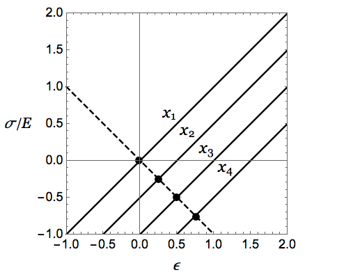
Figure 1: The constitutive behavior of the deposited material. The dashed line represents the “yield curve”, relating the initial stress with the total strain at deposition. The solid lines represent the elastic stress-strain curves for 4 material points deposited at $x_{1}=0$, $x_{2}=0.25$, $x_{3}=0.5$, $x_{4}=0.75$. They keep the memory of the initial state at deposition shown by the black circles. Here $L=1$, $C=-1$.

IV 1.5D problem

The goal of our second example is to create room for incompatibility without compromising the analytical transparency of the 1D setting. To this end we assume that the bar is laterally constrained by an elastic background, composed of leaf (shear) springs attached to a rigid wall. We will refer to such compound system as a “1.5D bar” because the problem remains to be ODE based.

Incompatibility. Consider first a fixed length 1.5D bar in a stress-free reference configuration $\mathscr{B}=\left\{x\,|\,0\leq x\leq L\right\}$. Denote by $u(x)$ the displacement field in $\mathscr{B}$ and by $\mathring{u}$ the shift of the attachment points of the shear springs relative to the background. Then the bar is subjected to a distributed live loading by the body forces $q(x)=-k(u(x)-\mathring{u}(x)).$ If no other loads act on the bar, equilibrium equations read

$$\left\{\begin{array}[]{lll}\sigma^{\prime}(x)+q(x)=0\\ \sigma(0)=\sigma(L)=0.\end{array}\right.$$ (21)

Supplementing this system by the constitutive relations $\sigma(x)=E(u^{\prime}(x)-\varepsilon_{p}(x))$ and eliminating $u$ we obtain

$$\sigma^{\prime\prime}(x)-\beta^{2}\sigma(x)=k(\varepsilon_{p}(x)-\mathring{u}^{\prime}(x))$$ (22)

where we have set $\beta^{2}=k/E$. Observe that $\beta$ has a dimension of inverse length scale and that the dimensionless ratio $\bar{\beta}=\beta L$ characterizes the role of elastic foundation: if $\bar{\beta}$ is small, the foundation can be neglected and if $\bar{\beta}$ is large the foundation dominates the response.

Observe also that Eq. (22) is the 1.5D counterpart of (13)_1,2, and that the function

$$\eta(x)=\varepsilon_{p}(x)-\mathring{u}^{\prime}(x)$$ (23)

can be viewed as the analog of incompatibility in this problem: a measure of the mismatch between the “external” (non-1D) and the “internal” (1D) pre-strains, cf. Basile17 . For instance, the residual stresses in this setting are defined by $\eta(x)$ rather than $\varepsilon_{p}(x)$ and even if $\varepsilon_{p}=0$ there may be equally “inelastic” strains $\mathring{u}^{\prime}$ in the system.

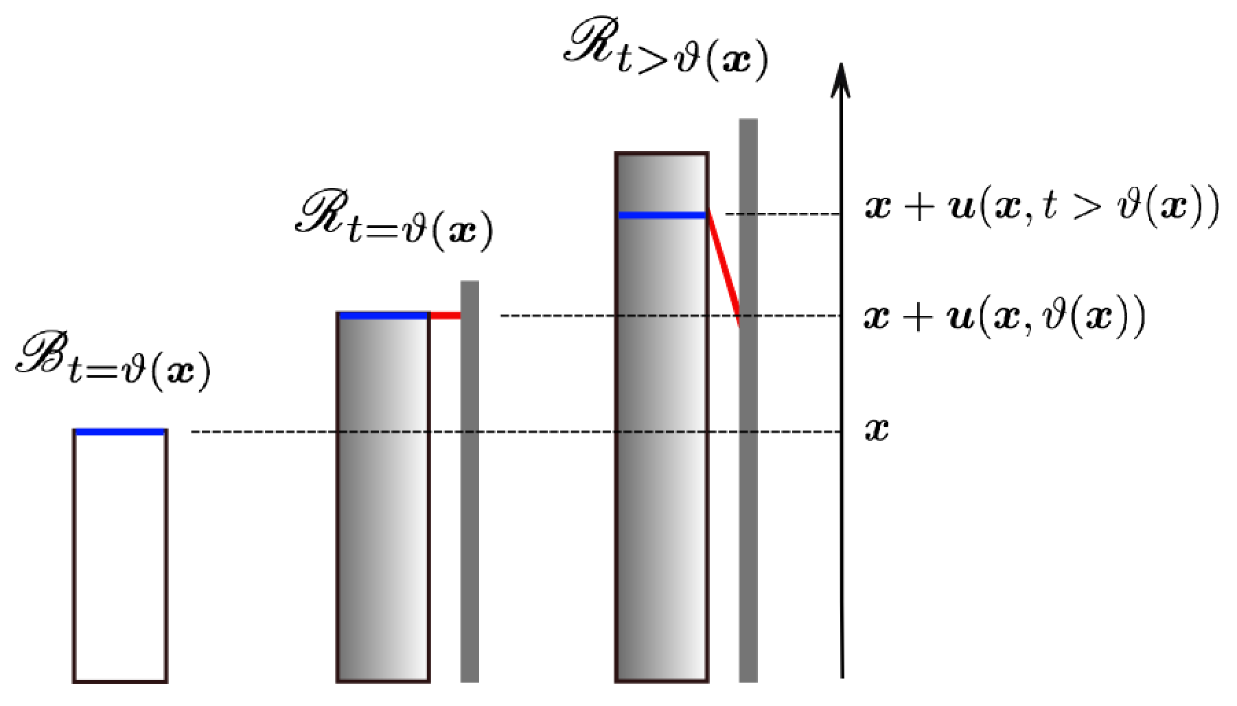
Figure 2: At the moment of deposition $t=t(x)$, the point $x$ (blue line) in the reference state occupies position $x+\mathring{u}(x))$ in the actual state. A shear spring (red line) is created at this instant, linking point $x$ to the background. At time $t>\vartheta(x)$ the point $x$ is no longer at the accretion surface and the spring is no longer undeformed.

Surface growth. Without loss of generality we can assume that the connecting springs are in a stress-free state at deposition so that $\mathring{u}(x))=u(x,\vartheta(x))$ and $q(x,\vartheta(x))=0$, see Fig. 2. Suppose also that the end $x=0$ is constrained and that the bar is exposed to the foundation-unrelated body forces $b(x)$ and the tractions $s(x)$ on the growing end. Then the equilibrium equations at time $t$ read

$$\left\{\begin{array}[]{llll}\partial_{x}\sigma(x,t)+k(\mathring{u}(x)-u(x,t))+b(x)=0&\mathscr{B}_{t}\\ \sigma(x,t)=E(\partial_{x}u(x,t)-\varepsilon_{p}(x))&\mathscr{B}_{t}\\ \sigma(\psi(t),t)=s(\psi(t))&\Omega_{t}\\ u(0,t)=0&\Omega_{d}.\end{array}\right.$$ (24)

If $\varepsilon_{p}(x)$ is prescribed, this linear problem can be solved analytically, in particular we obtain explicit representations

$$\begin{array}[]{llll}\displaystyle\mathring{u}^{\prime}(x)&=\varepsilon_{p}(x)+\displaystyle\frac{\beta s(x)+(s^{\prime}(x)+b(x))\tanh(\beta x)}{\beta E},\\ \displaystyle\eta(x)&=\displaystyle-\frac{\beta s(x)+(s^{\prime}(x)+b(x))\tanh(\beta x)}{\beta E}.\end{array}$$ (25)

If, instead, $\varepsilon_{p}(x)$ is unknown, we need to prescribe a supplementary condition on the growing end. For instance, by prescribing $\mathring{u}$, as we did in the 1D case, we obtain

$$\varepsilon_{p}=\mathring{u}^{\prime}-\frac{s}{E}-\frac{\tanh(\beta x)}{\beta E}(s^{\prime}+b).$$ (26)

Incremental approach. It is instructive to see how the incremental approach works in the 1.5D case. We can again define

$$\begin{array}[]{lll}u(x,t)=\mathring{u}(x)+\int_{\vartheta(x)}^{t}\dot{u}(x,z)\,dz\\ \sigma(x,t)=s(x)+\int_{\vartheta(x)}^{t}\dot{\sigma}(x,z)\,dz.\end{array}$$ (27)

and formulate the incremental equilibrium problem

$$\left\{\begin{array}[]{lccc}\partial_{x}\dot{\sigma}(x,t)-k\dot{u}(x,t)=0&\mathscr{B}_{t}\\ \dot{\sigma}(x,t)=E\,\partial\dot{u}(x,t)&\mathscr{B}_{t}\\ \dot{u}(0,t)=0&\Omega_{d}.\end{array}\right.$$ (28)

The boundary condition on the growing end takes the form

$$\dot{\sigma}(x,t)\big{|}_{t=\vartheta(x)}=D_{0}(x)\left(s^{\prime}(x)+b(x)\right).$$ (29)

The incremental problem (28)-(29) is the 1.5D counterpart of the 3D problem (6)-(8). If we set $\psi\equiv t$ for simplicity, so that $\vartheta(x)=x$ and $D_{0}=1$, we can write the incremental solution explicitly

$$\dot{u}(x,\psi)=\text{sech}(\beta\psi)\sinh(\beta x)(s^{\prime}(\psi)+b(\psi))/(E\beta).$$ (30)

After computing the incremental stress from (28)₂, we obtain from (27)₂ the explicit representation of the stress field

$$\sigma(x,\psi)=s(x)+\text{cosh}(\beta x)\int_{x}^{\psi}(s^{\prime}(z)+b(z))\,\text{sech}\,(\beta z)\,dz.$$ (31)

Note that we found the stress without knowing either the inelastic strain $\varepsilon_{p}(x)$ or the displacement $\mathring{u}(x)$.

If $\varepsilon_{p}$ is known, we can now integrate $\sigma(x,\psi)=E(\partial u(x,\psi)-\varepsilon_{p}(x))$ with a boundary condition $u(0,\psi)=0$ and find the displacement field $u(x,\psi)$. This gives us $\mathring{u}(\psi)=u(\psi,\psi)$ in full agreement with (25). If $\varepsilon_{p}(x)$ is unknown but either $\mathring{u}(x)$ or $D(x)$ are prescribed, the same Eq. (25) can be used to compute the inelastic strain.

V Illustrations

1.5D printing. Consider a printing device that can control the ratio $D/D_{0}$ during deposition and assume for simplicity the bar is elastic, so that $\varepsilon_{p}=0$. In this case the inelastic effects are due exclusively to the external pre-strain $\mathring{u}^{\prime}$.

If the target is a prescribed distribution of residual stress $\bar{\tau}(x)$ satisfying $\bar{\tau}(0)=\bar{\tau}(L)=0$, we can use (22) to compute the target incompatibility

$$\bar{\eta}=\left(\bar{\tau}^{\prime\prime}-\beta^{2}\bar{\tau}\right)/k.$$ (32)

The corresponding deposition protocol is then given by the equation

$$D/D_{0}-1=\left(\beta^{2}\bar{\tau}-\bar{\tau}^{\prime\prime}\right)/k.$$ (33)

The inverse problem can be solved similarly. Thus, if we assume that $D/D_{0}$ is given and integrate (33) with boundary conditions $\tau(0)=\tau(L)=0$, we obtain the resulting distribution of residual stresses. If, for example, the velocities $D,D_{0}$ are both constant, we obtain

$$\tau=\left(\small{\frac{D}{D_{0}}}-1\right)(1-\cosh(\beta x)+\frac{\sinh(\beta x)\tanh(\beta L/2))}{\beta^{2}}.$$ (34)

This stress distribution, illustrated in Fig.3, vanishes if $D=D_{0}$, however, when $D>D_{0}$ the grown bar is left in a state of residual traction while for $D<D_{0}$, the residual stresses are compressive.

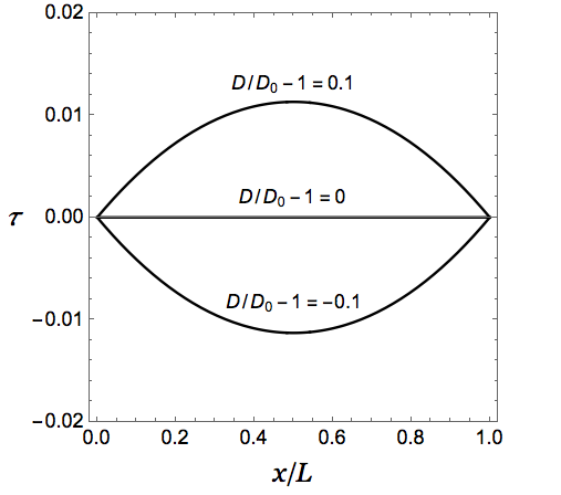
Figure 3: Residual stresses in a 1.5D bar printed with controlled mismatch between Lagrangian and Eulerian velocities of the growing surface. Here $\beta=1$ and $L=1$.

Brick tower. Consider a tower built by continuous deposition of “bricks” on one of its ends, while the other end is fixed. The tower is supported by a vertical wall to which the upcoming bricks are attached. We first illustrate the role of the body force distribution $b(x)$.

We compare two protocols: when the forces $b$ are present in the process of growth, and when they are introduced only after the growth process is completed. We can think about one brick tower manufactured vertically (under the continuous action of gravity) and another brick tower manufactured horizontally (in absence of gravity), and then turned vertically at the end of manufacturing. In both cases we assume that $s=0$ on the growing end, and neglect plastic strains in the bar.

In the first case (vertical tower) we have $b=-\rho g$, where $\rho$ is the linear mass density and $g$ is the acceleration of gravity. Then, from (23) and (25) we obtain

$$\eta(x)=\frac{\rho g\tanh(\beta x)}{\beta E},$$ (35)

and, from (31), the final stress distribution reads

$$\sigma(x)=\frac{\rho g}{\beta}\text{cosh}(\beta x)\left(\text{gd}(\beta x)-\text{gd}(\beta L)\right),$$ (36)

where $\text{gd}(x)=2\,\text{arctan}(\text{tanh}(x/2))$. In the limit $\beta\rightarrow 0$, when the foundation can be neglected, we obtain an elastic growth with $\eta(x)=0$ and $\sigma(x)=-\rho g(L-x)$. In the limit $\beta\rightarrow\infty$ the foundation dominates and carries the applied loads, so that the bar is stress free.

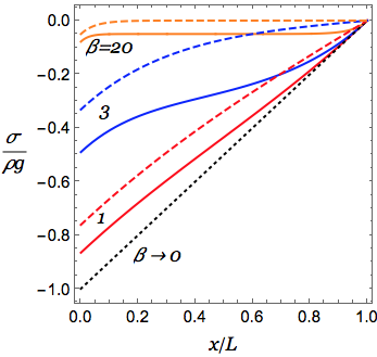
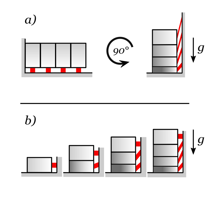
Figure 4: Dashed curves: stress distribution in the structure subjected to gravity after it is manufactured, see also (a). Continuous curves: stress in the structure manufactured under the action of gravity, see also ( b). The curves are distinguished by the value of the parameter $\beta$. The dotted line represents the stress in the limiting case when there is no foundation.

In the second case, we manufacture the tower without gravity while assuming that $D=D_{0}$, so that $\eta=0$. If we now rotate the structure (switch on gravity) the stress distribution can be found from (21) with boundary conditions $\sigma(L)=0$ and $u(0)=0$. With $b=-\rho g$ we obtain

$$\sigma(x)=-\frac{\rho g}{\beta}\text{sech}(\beta L)\text{sinh}(\beta(L-x)).$$ (37)

Also in this case, the purely elastic solution is recovered in the statically determined limit $\beta\rightarrow 0$, while in the limit $\beta\rightarrow\infty$ the stress in the bar drops to zero, as the applied load is fully carried by the foundation.

The stress distributions in the two brick towers, one manufactured vertically and the other one manufactured horizontally and then rotated, are illustrated in Fig.4. A comparison of the stress profiles at the same values of $\beta$ shows that the distributions are different, which highlights the inherent path dependence of the process of incompatible surface growth.

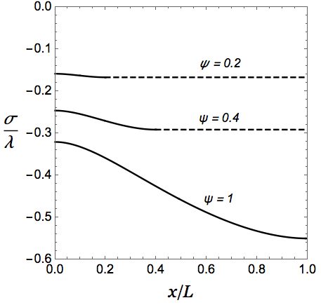
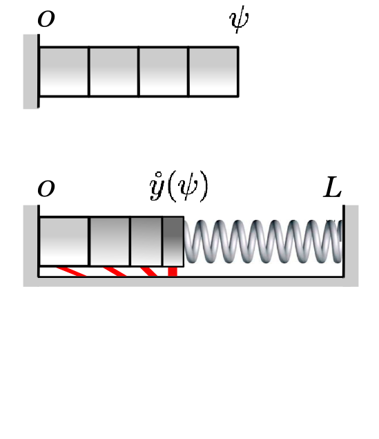
Figure 5: Left: stress in the bar (solid) and in the spring (dashed) for different positions $\psi/L$ of the interface, for $\beta=3$ and $\alpha=1$. Right: Reference (up) and current (down) configurations of the the growing bar, for a specific value of $\psi$.

Growth against an elastic constraint. Finally, consider a bar growing against an elastic constraint while the non-growing end is kept fixed. Also in this case we assume for analytical transparency that $\varepsilon_{p}=0$ and neglect body forces. The traction $s$ exerted by the elastic constraint depends on the current position $\mathring{y}(\psi)=\psi+\mathring{u}(\psi)$ of the accreting surface, so if $s=\bar{s}(\psi+\mathring{u}(\psi))$ is known, (25)₁ can be viewed as a first order ordinary differential equation for $\mathring{u}$, that can be integrated with an initial condition $\mathring{u}(0)=0$. For instance, if the growth resisting elastic force is linear $\bar{s}(z)=-\lambda z/L,$ where $\lambda$ is an elastic constant, integration gives

$$\begin{array}[]{lll}&\mathring{u}(x)=L\alpha^{-1}-x\\ &-e^{xLm\beta^{2}}L\alpha^{-1}\beta^{m}(\beta L\cosh(\beta x)+\alpha\sinh(\beta x))^{m}\end{array}$$ (38)

where we have set $\alpha=\lambda/E$ and $m=\alpha^{2}/(\alpha^{2}-L^{2}\beta^{2})$. We can now compute the surface traction $s$ and, by making use of (31), obtain the stress in the system. The results, illustrated in Fig.5, show that surface growth in this setting can produce highly inhomogeneous stress fields.

VI Conclusions

In this paper we have developed a non-incremental theory of inelastic surface growth allowing one to compute the distribution of plastic strains that were underplayed in the incremental approach presented in ZT17 . To illustrate the new ideas, we presented several analytically transparent examples where the general theory was applied to the growth of bars attached to a Winkler foundation. By explicit solutions we demonstrated the path-dependence of the process of inelastic growth and highlighted different roles played in the theory by compatible and incompatible inelastic strains. Surface growth in such 1.5D systems is of interest in various applications, for instance, in civil engineering of high-rise construction, in the study of self-propulsion of cells on rigid substrates and in micro-technologies based on “de-peeling” of programmable structures with non-trivial relaxed shapes.

References

- (1) Goriely A., The Mathematics and Mechanics of Biological Growth, Springer-Verlag New York (2017).
- (2) Tomassetti G., Cohen T., Abeyaratne R., Steady accretion of an elastic body on a hard spherical surface and the notion of a four-dimensional reference space, J. Mech. Phys. Solids, 96, 333–352 (2016).
- (3) Skalak R., Hoger A., Kinematics of surface growth. J. Math. Biol. 35, 869–907 (1997).
- (4) Di Carlo A., Quiligotti S., Growth and balance, Mech. Res. Comm., 29, 449–456 (2002).
- (5) Ciarletta P., Preziosi L., Maugin G.A., Mechanobiology of interfacial growth, J. Mech. Phys. Solids, 61, 852–872 (2013).
- (6) Epstein M., Maugin G.A., Thermomechanics of volumetric growth in uniform bodies, Int.J.Plast., 16, 951–978 (2000).
- (7) Maugin G.A., Configurational forces: thermomechanics, physics, mathematics, and numerics, CRC Press, Taylor Francis Group, Boca Raton London New York (2011).
- (8) Ambrosi D., Guana F., Stress-Modulated Growth, Math. Mech. Sol., 12, 319–342 (2007).
- (9) Yavari A., A geometric theory of growth mechanics. J. Nonlinear Sci. 20, 781–830 (2010).
- (10) Kuhl E., Holzapfel G.A., A continuum model for remodeling in living structures, J. Mater. Sci. 42(21), 8811–8823 (2007).
- (11) Ben Amar M., Goriely A., Growth and instability in elastic tissues, J. Mech. Phys. Solids 53, 2284–2319 (2005).
- (12) Jones G.W., Chapman S.J., Modeling Growth in Biological Materials, SIAM Review, 54(1), 52–118 (2012).
- (13) Ateshian G.A. , On the theory of reactive mixtures for modeling biological growth, Biomech. Model. Mechan., 6, 423–445 (2007).
- (14) Brown C.B., Goodman L.E., Proc.Royal Soc. London Sez.A, Math. and Phys. Sci., 276(1367), 571–576 (1963).
- (15) King W.D., Fletcher N.H., J.Phys.D: Appl.Phys. 6(18), 21–57 (1973).
- (16) Trincher V.K., Izv. AN SSSR. Mekhanika Tverdogo Tela, 19(2) 119-124 (1984).
- (17) Naumov V. E., Mechanics of growing deformable solids: a review, J. Eng. Mech.,120, 207-220 (1994).
- (18) Arutyunyan N. Kh., Metlov V. V.,Izv. Akad. Nauk SSSR, Mekh. Tverd. Tela 4, 142–152 (1983).
- (19) Bacigalupo A., Gambarotta L., Mechanics Based Design of Structures and Machines 40, 163–184 (2012).
- (20) Sozio F., Yavari A., Nonlinear mechanics of surface growth for cylindrical and spherical elastic bodies, JMPS 98, 12-48 (2017).
- (21) Hodge N. Papadopoulos P., A continuum theory of surface growth, Proc. R. Soc. A 466, 3135-3152 (2010).
- (22) Zurlo G., Truskinovsky L., Printing Non-Euclidean Solids, Phys. Rev. Lett., 119, 048001 (2017).
- (23) Kondaurov, V.I., Nikitin, L.V., Finite strains of viscoelastic muscle tissue. PMM J. Appl. Math. Mech. 51, 346-353 (1987).
- (24) Danescu A., Chevalier C., Grenet G., Regreny Ph., Letartre X., Leclercq J. L., Appl. Phys.Lett. 102, 123111 (2013).
- (25) Markenscoff X., Gupta A., Configurational balance laws for incompatibility in stress space, Proc. R. Soc. A 2007 463, 1379-1392 (2007).
- (26) Lestringant C., Audoly B., Elastic rods with incompatible strain: macroscopic versus microscopic buckling, JMPS (2017).