Chromatic splitting for the $K(2)$-local sphere at $p=2$

Abstract.

We calculate the homotopy type of $L_{1}L_{K(2)}S^{0}$ and $L_{K(1)}L_{K(2)}S^{0}$ at the prime 2, where $L_{K(n)}$ is localization with respect to Morava $K$-theory and $L_{1}$ localization with respect to $2$-local $K$ theory. In $L_{1}L_{K(2)}S^{0}$ we find all the summands predicted by the Chromatic Splitting Conjecture, but we find some extra summands as well. An essential ingredient in our approach is the analysis of the continuous group cohomology $H^{\ast}_{c}(\mathbb{G}_{2},E_{0})$ where $\mathbb{G}_{2}$ is the Morava stabilizer group and $E_{0}={{\mathbb{W}}}[[u_{1}]]$ is the ring of functions on the height $2$ Lubin-Tate space. We show that the inclusion of the constants ${{\mathbb{W}}}\to E_{0}$ induces an isomorphism on group cohomology, a radical simplification.

1. Introduction

The problem of understanding the homotopy groups of spheres has always been central to algebraic topology. A period of calculation beginning with Serre’s computation of the cohomology of Eilenberg- MacLane spaces and Toda’s work with the EHP sequence culminated, in the late 1970s, with the work of Miller, Ravenel, and Wilson on periodic phenomena in the homotopy groups of spheres and Ravenel’s nilpotence conjectures. The solutions to most of these conjectures in the middle 1980s established the primacy of the chromatic point of view, which uses the algebraic geometry of smooth $1$-parameter formal groups to organize the search for large scale phenomena in stable homotopy theory.

This has been remarkably successful. Much of what we know about stable homotopy theory can be motivated and conjectured by analyzing the moduli stack of formal groups and its quasi-coherent sheaves. See, for example, the table in Section 2 of [HG94]. In particular, this stack has a stratification by height and working along this stratification highlights two distinct lines of research. First, we’d like to discover all that can be learned by working at a single height; or, put another way, we make calculations in $K(n)$-local homotopy theory. Second, we need to assemble the information from different heights. This is the chromatic assembly problem.

In this paper, we give an analysis of the Chromatic Splitting Conjecture of Hopkins at $p=2$ and $n=2$. At first glance, this is a chromatic assembly question, but as we proceed here we need extensive information from height 2 calculations. Thus, the questions of single-height calculations and chromatic assembly remain closely related.

The Chromatic Splitting Conjecture predicts a splitting of $L_{1}L_{K(2)}S^{0}$. We do get a splitting, and it contains the expected summands, but it contains other summands as well. That there has to be more was already proved in [Bea17a], which in turn builds on the papers [Bea15] and [Bea17b], all by the first author. There are hints at extra summands in the work of Shimomura and Wang [Shi99, SW02] as well. This is discussed in 1.1.4.

Fix a prime $p$ and let $K(n)$ be the $n$th Morava $K$-theory spectrum; by convention, $K(0)=H\mathbb{Q}$, the rational homology spectrum. Let $L_{n}$ be localization with respect to the homology theory represented by $K(0)\vee K(1)\vee\cdots\vee K(n)$. This is the same as localization with respect to the Johnson-Wilson theory $E(n)$. Then for all spectra $X$ there is a natural localization map $L_{n}X\to L_{n-1}X\simeq L_{n-1}L_{n}X$. The Hopkins-Ravenel Chromatic Convergence Theorem of §8.6 of [Rav92] then says that if $X$ is a finite CW spectrum the induced map

$$X{{\longrightarrow\ }}\operatorname{holim}L_{n}X$$

is localization at the homology theory $H_{\ast}(-,{{\mathbb{Z}}}_{(p)})$.

Next, let $L_{K(n)}X$ be localization with respect to $K(n)$. Then the $K(n)$-localization of $L_{n}X$ is a map $L_{n}X\to L_{K(n)}X$ and, for any spectrum $X$, the natural map $L_{n}X\to L_{n-1}X$ can be recovered from the chromatic fracture square

(1.1.1)

That this square is a homotopy pull-back can be found in Theorem 6.19 of [HS99], but is implicit in [Rav84] as well.

The chromatic fracture square and chromatic convergence together imply that we can recover the homotopy type of a finite CW spectrum from $L_{K(n)}X$ for all $n$ and all $p$, provided we can complete the assembly process of (1.1.1).

Calculations of $L_{K(n)}X$ usually come down to analysis of the $K(n)$-local Adams-Novikov Spectral Sequence. The cohomology theory $K(n)^{\ast}$ is complex orientable and the associated formal group $\Gamma_{n}$ is of height $n$. Let $\mathbb{G}_{n}$ be the automorphisms of the pair $(\mathbb{F}_{p^{n}},\Gamma_{n})$ and let $E_{n}$ be the Morava $E$-theory associated to the pair $(\mathbb{F}_{p^{n}},\Gamma_{n})$. By the Goerss-Hopkins-Miller Theorem the profinite group $\mathbb{G}_{n}$ acts on $E_{n}$, and hence on $(E_{n})_{\ast}X:=\pi_{\ast}L_{K(n)}(E_{n}\wedge X)$. If $X$ is a finite CW spectrum, we then have a spectral sequence

(1.1.2) $$H_{c}^{s}(\mathbb{G}_{n},(E_{n})_{t}X)\Longrightarrow\pi_{t-s}L_{K(n)}X$$

where cohomology is continuous group cohomology. Much of $K(n)$-local homotopy theory comes down to the analysis of the group $\mathbb{G}_{n}$ and the action of $\mathbb{G}_{n}$ on $(E_{n})_{\ast}$. We give some more details in Section 2 and add references to the large literature on the subject there.

Even assuming we can master the $K(n)$-local calculations, there remains the assembly question. Let $M_{n}X$ be the fiber of $L_{n}X\to L_{n-1}X$; then the key result needed to establish the chromatic fracture square of (1.1.1) is that the induced map $M_{n}X\to M_{n}L_{K(n)}X$ is an equivalence. Crucial to assembly is the other fiber; that is, the fiber of $L_{n-1}X\to L_{n-1}L_{K(n)}X$. This is the main subject of this paper. In fact, we investigate the homotopy type of the map $L_{n-1}X\to L_{n-1}L_{K(n)}X$. The Chromatic Splitting Conjecture, due to Hopkins, is a very specific conjecture about this map. We will get into this below; before that, however, we will state our main results.

Let $p=2$ and write $E=E_{2}$ for our choice of Morava $E$-theory at height $2$. Let ${{\mathbb{W}}}$ be the Witt vectors on $\mathbb{F}_{4}$. Then there is an isomorphism $E_{\ast}\cong{{\mathbb{W}}}[[u_{1}]][u^{\pm 1}]$ where the power series ring is in degree $0$ and $u$ has degree $-2$. Our first result is a $K(2)$-local result. See 6.1.1 and 6.1.4

Theorem 1.1.1.

The inclusion of constants into the power series ring induce isomorphisms in group cohomology

$$H_{c}^{*}(\mathbb{G}_{2},\mathbb{F}_{4})\to H_{c}^{*}(\mathbb{G}_{2},E_{0}/2)$$

and

$$H_{c}^{*}(\mathbb{G}_{2},{{\mathbb{W}}})\to H_{c}^{*}(\mathbb{G}_{2},E_{0}).$$

This is a remarkable simplification. We conjecture that the analogous result is true at all heights and all primes.

Conjecture 1.1.2 (Chromatic Vanishing Conjecture).

For any prime $p$ and height $n$, the inclusion of constants into the power series ring induces isomorphisms in group cohomology

$$H_{c}^{*}(\mathbb{G}_{n},\mathbb{F}_{p^{n}})\to H_{c}^{*}(\mathbb{G}_{n},\pi_{0}E_{n}/p)$$

and

$$H_{c}^{*}(\mathbb{G}_{n},{{\mathbb{W}}})\to H_{c}^{*}(\mathbb{G}_{n},\pi_{0}E_{n})$$

We call this the Chromatic Vanishing Conjecture as it implies and is implied by the vanishing of the cohomology groups $H_{c}^{*}(\mathbb{G}_{n},(\pi_{0}E_{n}/p)/\mathbb{F}_{p^{n}})$ and $H_{c}^{*}(\mathbb{G}_{n},(\pi_{0}E_{n})/\mathbb{W})$ in all degrees.

This conjecture is true wherever it has been checked; that is, for $n\leq 2$ and all primes. If $n=1$ this is a tautology. For $n=2$ and $p>3$, it can be deduced from [SY95] (see also Corollaire 4.5 of [Lad13]). This basic case was also proved later in [Koh13] using different techniques. For $n=2$ and $p=3$ it can be deduced from [HKM13]; [GHM14]. The primes $2$ and $3$ are harder, as the group $\mathbb{G}_{2}$ contains $p$-torsion subgroups.

The next step is to calculate differentials in the Adams-Novikov spectral sequence (1.1.2) for $X=S^{0}$. By an old result of Lazard, applied by Morava in our case [Laz65, Mor85], we know that for all $n$ and $p$ the cohomology ring $H_{c}^{*}(\mathbb{G}_{n},{{\mathbb{W}}})\otimes\mathbb{Q}$ is an exterior algebra on $n$ generators of degree $2i-1$ for $1\leq i\leq n$; then 1.1.1 implies $\pi_{i}L_{K(2)}S^{0}$ has a torsion-free generator when $i=0$, $-1$, $-3$, or $-4$. To get further, we need to get some control on the torsion.

For all $n$ and $p$, the group $\mathbb{G}_{n}$ comes equipped with a determinant map

$$\det\colon\mathbb{G}_{n}\to{{\mathbb{Z}}}_{p}^{\times}$$

to the units in the $p$-adic integers. If $p=2$, there is an isomorphism ${{\mathbb{Z}}}_{2}^{\times}\cong{{\mathbb{Z}}}_{2}\times C_{2}$, where $C_{2}=\{\pm 1\}$ is the cyclic group of order $2$. We thus get a map

$$E(\zeta_{2})\otimes\mathbb{F}_{2}[{{\chi}}]\cong H_{c}^{\ast}({{\mathbb{Z}}}_{2}\times C_{2},\mathbb{F}_{2})\to H_{c}^{\ast}(\mathbb{G}_{2},\mathbb{F}_{2}).$$

Here $E(-)$ denotes the exterior algebra over $\mathbb{F}_{2}$. These cohomology classes will be discussed in 5.1.1. We will show in 5.3.1 (but see also Theorem 6.3.24 of [Rav86]), that this map induces an injection

Here is one place when the prime $2$ is fundamentally different. At odd primes, ${{\mathbb{Z}}}_{p}^{\times}\cong{{\mathbb{Z}}}_{p}\times C_{p-1}$, where $C_{p-1}$ is a cyclic group of order $p-1$. Thus, there is an isomorphism $H_{c}^{\ast}({{\mathbb{Z}}}_{p}^{\times},\mathbb{F}_{p})\cong E(\zeta_{2})$. The class ${{\chi}}$ only appears at $p=2$.

The class $\zeta_{2}$ is the reduction of a class of infinite order in $H_{c}^{1}(\mathbb{G}_{2},{{\mathbb{Z}}}_{2})$; that this class is a permanent cycle in the Adams-Novikov Spectral Sequence is well understood. In a standard abuse of notation we also write $\zeta_{2}\in\pi_{-1}L_{K(2)}S^{0}$ for a particular homotopy class detected by the cohomology class $\zeta_{2}$. See [DH04] and 2.2.1 for details. We will show that the Bockstein on the class ${{\chi}}$ is also a permanent cycle in $H_{c}^{2}(\mathbb{G}_{2},{{\mathbb{Z}}}_{2})$ and detects a class $x\in\pi_{-2}L_{K(2)}S^{0}$ of order $2$. We will then show that the Bockstein on $\zeta_{2}{{\chi}}$ detects the class $\zeta_{2}x\in\pi_{-3}L_{K(2)}S^{0}$, also of order $2$.

Let $V(0)$ be the mod $2$ Moore spectrum and let $\iota:S^{0}\to L_{K(2)}S^{0}$ be the unit. The classes $\iota$, $\zeta_{2}$, $x$ and $\zeta_{2}x$ together with choices for the torsion free generators of $\pi_{i}L_{K(2)}S^{0}$ for $i=-3$ and $i=-4$ can be used to define a map

(1.1.3) $$f:S^{0}\vee S^{-1}\vee S^{-3}\vee S^{-4}\vee\Sigma^{-2}V(0)\vee\Sigma^{-3}V(0){{\longrightarrow\ }}L_{K(2)}S^{0}$$

Our main result then describes chromatic splitting at $n=p=2$. Let $S^{n}_{2}$ denote the $2$-completed $n$-sphere.

Theorem 1.1.3.

The map $f$ defines a weak equivalence

$$L_{1}(S_{2}^{0}\vee S_{2}^{-1})\vee L_{0}(S_{2}^{-3}\vee S_{2}^{-4})\vee L_{1}(\Sigma^{-2}V(0)\vee\Sigma^{-3}V(0))\simeq L_{1}L_{K(2)}S^{0}.$$

In particular, $L_{1}S_{2}^{0}\rightarrow L_{1}L_{K(2)}S^{0}$ is a split inclusion.

Proving that the restriction of $f$ to $S^{-3}\vee S^{-4}$ factors through $L_{0}(S_{2}^{-3}\vee S_{2}^{-4})$ is part of the work necessary to prove the result. The spherical summands are predicted by the Chromatic Splitting Conjecture, but the Moore spectrum summands are the new phenomenon.

Remark 1.1.4.

Shimomura [Shi99] computes the Adams-Novikov $E_{2}$-term for $L_{2}V(0)$ and, with Wang [SW02], for $L_{2}S^{0}$ using the chromatic spectral sequence. For this reason, we cannot give a precise dictionary between our results. However, in Theorem 2.7 of [Shi99], the class $\zeta_{1}$ corresponds to the class we call $\chi$ later in this paper and gives rise to the Moore spectrum summands that are not predicted by the Strong Chromatic Splitting Conjecture. However, Shimomura and Wang do not compute the differentials in theses spectral sequences and their work settles neither the Strong nor Weak Chromatic Splitting Conjecture.

The strategy for proving 1.1.3 is to use the chromatic fracture square (1.1.1) to deduce the homotopy type $L_{1}L_{K(2)}S^{0}$. More precisely, we prove the following rational result. See 6.2.2 and 8.5.2.

Theorem 1.1.5.

Let $S^{n}_{2}$ be the $2$-complete $n$-sphere. Then the map $f$ of (1.1.3) induces a weak equivalence

$$L_{0}(S^{0}_{2}\vee S^{-1}_{2}\vee S^{-3}_{2}\vee S^{-4}_{2})\simeq L_{0}L_{K(2)}S^{0}.$$

Furthermore, we prove the following $K(1)$-local result. See 8.4.4.

Theorem 1.1.6.

The restriction of the map $f$ given in (1.1.3) to the wedge summand $S^{0}\vee S^{-1}\vee\Sigma^{-2}V(0)\vee\Sigma^{-3}V(0)$ induces a weak equivalence

$$L_{K(1)}\big{(}S^{0}\vee S^{-1}\vee\Sigma^{-2}V(0)\vee\Sigma^{-3}V(0)\big{)}\simeq L_{K(1)}L_{K(2)}S^{0}.$$

Much of the work in this paper goes into this last theorem. 1.1.3 then follows exactly as in the prime $3$ case; see [GHM14] and 8.5.2.

We conclude this introduction by revisiting the Chromatic Splitting Conjecture. This is due to Hopkins and can be found in the literature in [Hov95]. As we mentioned above, there is a result of Morava and Lazard that the cohomology ring $H_{c}^{*}(\mathbb{G}_{n},{{\mathbb{W}}})\otimes\mathbb{Q}$ is an exterior algebra on $n$ generators of degree $2i-1$ for $1\leq i\leq n$. Part of the Chromatic Splitting Conjecture is that, for some choice of generators $x_{i}\in H_{c}^{2i-1}(\mathbb{G}_{n},{{\mathbb{W}}})$, the exterior algebra $E_{{{\mathbb{Z}}}_{p}}(x_{1},\ldots,x_{n})$ over ${{\mathbb{Z}}}_{p}$ maps non-trivially to permanent cycles in $H_{c}^{*}(\mathbb{G}_{n},(E_{n})_{*})$. This would give a map out of a wedge of spheres to $L_{K(n)}S^{0}$ indexed on the monomial basis of the exterior algebra. The following would completely describe the gluing data (1.1.1).

Conjecture 1.1.7 (Strong Chromatic Splitting Conjecture).

This map out of the wedge of spheres induces an equivalence

$$L_{n-1}S_{p}^{0}\vee\bigvee_{1\leq i_{1}<\ldots<i_{j}\leq n}L_{n-i_{j}}S_{p}^{-2\left(\sum i_{k}\right)+j}\simeq L_{n-1}L_{K(n)}S^{0}\ .$$

The conjecture is known to hold for $n=1$ if $p\geq 2$ and for $n=2$ if $p\geq 3$ ([Beh12], [GHM14], [SY95]). However, the results of [Bea17a] already implies that 1.1.7 does not hold when $n=p=2$ and 1.1.3 makes this completely precise. We note that although 1.1.7 does not hold at $p=2$, there is no evidence that it should fail at odd primes, or at least when $p$ is large with respect to $n$. When $p=2$, our computations at $n=2$ beckon a reformulation of the Strong Chromatic Splitting Conjecture. We refer the reader to [Mil20, Section 5.6] for a discussion on this topic.

We can also write down a weaker form of the conjecture, which holds for all $p$ and $n\leq 2$; that is, for all cases where we’ve been able to check.

Conjecture 1.1.8 (Weak Chromatic Splitting Conjecture).

If $X$ is the $p$-completion of a finite spectrum, the map $L_{n-1}X\to L_{n-1}L_{K(n)}X$ is a split inclusion.

This second conjecture would imply that there are maps $L_{K(n)}S^{0}\rightarrow L_{K(n-1)}S^{0}$ such that $S^{0}\simeq\operatorname{holim}_{n}L_{K(n)}S^{0}$; that is, $S^{0}$ can be recovered from its Morava $K$-theory localizations.

Organization of the paper

In Section 2, we review some of the background from chromatic homotopy theory, including some of the more technical techniques at the prime $p=2$. In Section 3, we recall some classical results from homotopy theory; most of this can be summarized in the remark that extra care is needed because the order of the identity of the mod $2$ Moore spectrum is not equal to two. Then in Section 4 we give a detailed review of $K(1)$-local computations at the prime $p=2$ which are used in later sections. In Section 5, we begin our analysis of the case $n=p=2$. We describe the cohomology of various subgroups $G$ of $\mathbb{G}_{2}$. This is preliminary to Section 6, where we give the proof of 1.1.1 in 6.1.4. Section 7 is dedicated to one of the key technical results of the paper: the class ${{\chi}}$ is a $d_{3}$-cycle in the $K(2)$-local Adams-Novikov Spectral Sequence for the Moore spectrum. Section 8 contains the proof of 1.1.6. This theorem is shown by studying the $v_{1}$-localized Adams-Novikov Spectral Sequences computing $L_{K(1)}L_{K(2)}V(0)$ and especially $L_{K(1)}L_{K(2)}Y$ where $Y=V(0)\wedge C(\eta)$ for $C(\eta)$ the cofiber of $\eta\colon S^{1}\to S^{0}$. The spectrum $Y$ was used in Mahowald’s proof of the Telescope Conjecture at $p=2$ and $n=1$. See [Mah82]. We also deduce 1.1.3 and 1.1.5 at the end of Section 8.

We have been slightly disingenuous in our presentation above, as we actually prove 1.1.6 before constructing the map $f$ of (1.1.3); that is, we only construct the $K(1)$-localization of the map $f$ in Section 8. In Section 9 we complete the difficult task of constructing $f$.

Acknowledgements

This project had its genesis in conversations with Mark Mahowald, who was trying to come to terms with calculations of Shimomura and Wang [SW02]. Specifically, Mark thought that those authors had identified $v_{1}$-torsion-free summands in the $E_{2}$-term of the Adams-Novikov Spectral Sequence for $\pi_{\ast}L_{K(2)}V(0)$ which could not be explained by the Chromatic Splitting Conjecture. In some sense this entire paper, as well as [Bea17a] and [Bea17b], are an attempt to ratify and explain this insight.

Careful readers of Section 7 below will recognize that the techniques and ideas there are completely different from the rest of the paper. This lateral move arises from an insight of Mike Hopkins: namely, that the isomorphism of 1.1.1 could be extended to a homomorphism of homotopy fixed point spectral sequences. See the beginning of Section 7 for more details. We don’t completely prove that, but we do get enough information from this idea to prove our key 7.1.1. We extend heartfelt thanks to Hopkins for sharing this idea.

We also thank Mark Behrens, Irina Bobkova, Lars Hesselholt, Peter May and Zhouli Xu for useful conversations along the way, as well as two anonymous referees for their helpful comments.

Finally, this work has taken place over a number years and at a number of places. We thank the Hausdorff Institute of Mathematics, the Université de Strasbourg, and the University of Colorado Boulder all for providing such wonderful places to work.

2. Preliminaries

We begin by introducing the $K(n)$-local category, Morava $E$-theory, the Morava stabilizer group, and general convergence results for the $K(n)$-local Adams-Novikov Spectral Sequence. We then get specific at $n=2$ and $p=2$, discussing the role of formal groups from supersingular elliptic curves. We close the section with some background on algebraic and topological duality resolutions.

2.1. The $K(n)$-local category

Fix a prime $p$. Let $\Gamma_{n}$ be a formal group of height $n$ over the finite field $\mathbb{F}_{p}$ of $p$ elements and let $\mathop{\mathrm{End}}\nolimits(\Gamma_{n}/\mathbb{F}_{p})$ be the endomorphism ring of $\Gamma_{n}$ over $\mathbb{F}_{p}$. This ring is in fact the maximal order in a central division algebra over $\mathbb{Q}_{p}$ of Hasse invariant $1/n$ (see for example Appendix A.2 of [Rav86]). The unique map of rings ${{\mathbb{Z}}}_{p}\to\mathop{\mathrm{End}}\nolimits(\Gamma_{n}/\mathbb{F}_{p})$ is an inclusion into the center. Because $\Gamma_{n}$ is defined over $\mathbb{F}_{p}$ the Frobenius map $\xi(x)=x^{p}$ also defines an endomorphism of $\Gamma_{n}$. We will assume the endomorphism $\xi^{n}(x)=x^{p^{n}}$ satisfies an equation

(2.1.1) $$\xi^{n}(x)=[ap](x)\in\mathop{\mathrm{End}}\nolimits_{\mathbb{F}_{p^{n}}}(\Gamma_{n}/\mathbb{F}_{p})$$

where $a\in{{\mathbb{Z}}}_{p}^{\times}$ is a unit and $[\ell](x)$ denotes the $\ell$-series for $\ell\in{{\mathbb{Z}}}_{p}$. The Honda formal group of height $n$ satisfies these criteria: this has a formal group law which is $p$-typical and with $p$-series $[p](x)=x^{p^{n}}=\xi^{n}(x)$. However, if $n=2$ and $p=2$, then the formal group of a supersingular elliptic curve defined over $\mathbb{F}_{2}$ will also do, and this will be our preferred choice if $p=2$; see Section 2.4.

Let $i\colon\mathbb{F}_{p}\hookrightarrow k$ be any extension of $\mathbb{F}_{p}$ and let $\mathop{\mathrm{Aut}}\nolimits(\Gamma_{n}/k)$ be the group of automorphisms of $i^{\ast}\Gamma_{n}$ over $k$. Our assumption (2.1.1) implies that for any extension $\mathbb{F}_{p^{n}}\subseteq k$ there is an isomorphism

$$\mathop{\mathrm{Aut}}\nolimits(\Gamma_{n}/\mathbb{F}_{p^{n}})\mathop{\longrightarrow}^{\cong}\mathop{\mathrm{Aut}}\nolimits(\Gamma_{n}/k).$$

To shorten notation we define

(2.1.2) $$\mathbb{S}_{n}=\mathop{\mathrm{Aut}}\nolimits(\Gamma_{n}/\mathbb{F}_{p^{n}}).$$

If we choose a coordinate for $\Gamma_{n}$, then every element of $\mathbb{S}_{n}$ can be expressed as a power series $\phi(x)\in x\mathbb{F}_{p^{n}}[[x]]$ invertible under composition. The map $\phi(x)\mapsto\phi^{\prime}(0)$ defines a surjective map

$$\mathbb{S}_{n}\longrightarrow\mathbb{F}_{p^{n}}^{\times}.$$

We define $S_{n}$ to be the kernel of this map; this is the $p$-Sylow subgroup of the profinite group $\mathbb{S}_{n}$. The Teichmüller lift $\mathbb{F}_{p^{n}}^{\times}\to{{\mathbb{W}}}^{\times}\subseteq\mathbb{S}_{n}$ defines a section of this map, giving an isomorphism $S_{n}\rtimes\mathbb{F}_{p^{n}}^{\times}\cong\mathbb{S}_{n}$.

Define the extended Morava stabilizer group $\mathbb{G}_{n}$ as the automorphism group of the pair $(\mathbb{F}_{p^{n}},\Gamma_{n})$. Elements of $\mathbb{G}_{n}$ are pairs $(f,\phi)$ where $f\in\mathop{\mathrm{Aut}}\nolimits(\mathbb{F}_{p^{n}}/\mathbb{F}_{p})$ and $\phi\colon\Gamma_{n}\to f^{*}\Gamma_{n}$ is an isomorphism of formal groups. Since $\Gamma_{n}$ is defined over $\mathbb{F}_{p}$, there is an isomorphism

(2.1.3) $$\mathbb{G}_{n}\cong\mathop{\mathrm{Aut}}\nolimits(\Gamma_{n}/\mathbb{F}_{p^{n}})\rtimes\mathop{\mathrm{Gal}}\nolimits(\mathbb{F}_{p^{n}}/\mathbb{F}_{p})=\mathbb{S}_{n}\rtimes\mathop{\mathrm{Gal}}\nolimits(\mathbb{F}_{p^{n}}/\mathbb{F}_{p}).$$

We next define Morava $K$-theory; there are many variants, all of which have the same Bousfield class and define the same localization. To be specific, let $K(n)=K(\mathbb{F}_{p^{n}},\Gamma_{n})$ be the $2$-periodic ring spectrum with homotopy groups

$$K(n)_{\ast}=\mathbb{F}_{p^{n}}[u^{\pm 1}]$$

and with associated formal group $\Gamma_{n}$. Here the class $u$ is in degree $-2$. This slightly unclassical choice of $K(n)$ has the property that it receives a map $E_{n}\to K(n)$ from Morava $E$-theory defined below in (2.1.4).

We will spend a great deal of time working in the $K(n)$-local category and, when doing so, all our spectra will implicitly be localized. In particular, we emphasize that we will write $X\wedge Y$ for $L_{K(n)}(X\wedge Y)$, as this is the smash product internal to the $K(n)$-local category.

We now define the Lubin-Tate spectrum $E=E_{n}=E(\mathbb{F}_{p^{n}},\Gamma_{n})$. This is a complex oriented, Landweber exact, $2$-periodic, $E_{\infty}$-ring spectrum with

(2.1.4) $$E_{\ast}=(E_{n})_{\ast}\cong\mathbb{W}[[u_{1},\cdots,u_{n-1}]][u^{\pm 1}]$$

with $u_{i}$ in degree $0$ and $u$ in degree $-2$. Here $\mathbb{W}=W(\mathbb{F}_{p^{n}})$ is the ring of Witt vectors on $\mathbb{F}_{p^{n}}$. Note that $E_{0}$ is a complete local ring with residue field $\mathbb{F}_{p^{n}}$; the formal group over $E_{0}$ is a choice of universal deformation of the formal group $\Gamma_{n}$ over $\mathbb{F}_{p^{n}}$. (We will be specific about this choice at $n=p=2$ below in Section 2.4.) By the Goerss-Hopkins-Miller theorem, the group $\mathbb{G}_{n}=\mathop{\mathrm{Aut}}\nolimits(\Gamma_{n})\rtimes\mathop{\mathrm{Gal}}\nolimits(\mathbb{F}_{p^{n}}/\mathbb{F}_{p})$ acts on $E$ by maps of $E_{\infty}$-ring spectra [Rez98, GH04].

Definition 2.1.1.

If $X$ is a spectrum we let

$$E_{\ast}X=\pi_{\ast}L_{K(n)}(E\wedge X).$$

Warning 2.1.2.

Despite the notation, the functor $E_{\ast}(-)$ is not a homology theory, as it does not take wedges to sums in general. In [HS99], this is denoted by $E_{\ast}^{\vee}(-)$. Since it is our most important algebraic invariant intrinsic to the $K(n)$-local category, we use the simpler notation $E_{\ast}(-)$. Note that $E\wedge X\simeq L_{K(n)}(E\wedge X)$ whenever $X$ is a finite spectrum. However, $E_{*}E$ which we have defined to be $\pi_{*}L_{K(n)}(E\wedge E)$ is not isomorphic to $\pi_{*}(E\wedge E)$.

The $E_{\ast}$-module $E_{\ast}X$ is equipped with the $\mathfrak{m}$-adic topology where $\mathfrak{m}$ is the maximal ideal in $E_{0}$. This topology is always complete, but need not be separated in general. However, all the $E_{\ast}$-modules we consider in this paper will be complete and separated. For instance, sufficient conditions for the topology on $E_{*}X$ to be complete and separated are

1. if $E_{\ast}X$ is finitely generated as an $E_{*}$-module, or

2. if $K(n)_{*}X$ is concentrated in even degrees (Proposition 2.2 of [GHMR05]).

For all the spectra $X$ we consider in this paper, one of these two condition holds.

The action of $\mathbb{G}_{n}$ on $E_{n}$ determines a continuous action of $\mathbb{G}_{n}$ on $(E_{n})_{\ast}X$. If $n=1$, we can choose $E_{\ast}=K_{\ast}$, $p$-complete $K$-theory, and $\mathbb{G}_{1}={{\mathbb{Z}}}_{p}^{\times}$, the units in the $p$-adics. The action is then through the Adams operations and in that case we might write $\psi^{\ell}$ for the action of $\ell\in{{\mathbb{Z}}}_{p}^{\times}$; for example, as in (4.1.1). Not withstanding this, as general rule we will simply write $g_{\ast}$ for the action of $g\in\mathbb{G}_{n}$ on $E_{\ast}X$.

This action is twisted in the sense that if $g\in\mathbb{G}_{n}$, $a\in E_{\ast}$ and $x\in E_{\ast}X$, then $g_{\ast}(ax)=g_{\ast}(a)g_{\ast}(x)$. We will call such modules either Morava modules or twisted $E_{*}$-$\mathbb{G}_{n}$-modules. When we consider closed subgroups $H$ of $\mathbb{G}_{n}$ and $E_{*}$-modules with an action of $H$ satisfying the analogous formula for $h\in H$ then we call such modules twisted $E_{*}$-$H$-modules. See Section 1.3 [BG18] for a more lengthy discussion on Morava modules.

The $E_{\ast}$-algebra $E_{\ast}E$ has a $\mathbb{G}_{n}$-action on both the left and right factor. The action of the left factor defines the Morava module structure. Using the action on the right factor we get a composite map

where $m$ is induced by the multiplication $E\wedge E\to E$. The adjoint to this map is an isomorphism

(2.1.5) $$E_{\ast}E\cong\operatorname{map}_{cts}(\mathbb{G}_{n},E_{\ast})$$

of Morava modules. Here $\operatorname{map}_{cts}(-,-)$ denotes the set of continuous maps. On the right hand side of this equation, $E_{\ast}$ acts on the target and the $\mathbb{G}_{n}$-action is the diagonal action given by $(g_{\ast}\phi)(x)=g_{\ast}\phi(g_{\ast}^{-1}x)$.

Caution is needed here. The isomorphism (2.1.5) need not hold for the Lubin-Tate homology theory $E(k,\Gamma)$ for an arbitrary height $n$ formal group $\Gamma$ over a field $k\subseteq\overline{\mathbb{F}}_{p}$. In the literature (2.1.5) is proved for the Honda formal group; see, for example, Theorem 12 of [Str00, DH04, Hov04]. In examining the proof there we see that what is needed is our assumption from (2.1.1). The details needed to then produce the isomorphism of (2.1.5), and more information as well, can be found in §5 of [Hen18].

Now suppose $X$ is a finite $p$-local spectrum. From (2.1.5) it follows (again see [Str00]) that the $K(n)$-local $E$-based Adams Spectral Sequence for $X$ has the form

(2.1.6) $$H_{c}^{s}(\mathbb{G}_{n},E_{t}X)\Longrightarrow\pi_{t-s}L_{K(n)}X.$$

Group cohomology here is continuous group cohomology. There is extensive discussion of this spectral sequence in [DH04].

Complex orientations define maps of ring spectra

If we localize at a prime and if $X$ is a finite $p$-local spectrum, we get a diagram of spectral sequences where the upward arrows are isomorphisms

(2.1.7)

For example, let $F\subseteq\mathbb{G}_{n}$ be a closed subgroup. In [DH04] Devinatz and Hopkins defined and studied a homotopy fixed point spectrum $E^{hF}$ with the property that the isomorphism of (2.1.5) descends to an isomorphism of Morava modules

(2.1.8) $$E_{\ast}E^{hF}\cong\operatorname{map}_{cts}(\mathbb{G}_{n}/F,E_{\ast})$$

and a spectral sequence for $X$ a finite CW spectrum

(2.1.9) $$H_{c}^{s}(F,E_{t}X)\Longrightarrow\pi_{t-s}(E^{hF}\wedge X)\ .$$

If $F=\mathbb{G}_{n}$ itself this spectral sequence is the $K(n)$-local Adams-Novikov Spectral Sequence for $L_{K(n)}S^{0}$ and, if $F$ is finite, this spectral sequence is the homotopy fixed point spectral sequence for the action of $F$ on $E$. The Devinatz-Hopkins construction is natural in $F$ and, in particular, if $F_{1}\subseteq F_{2}$ are two closed subgroups, we have a commutative diagram of spectral sequences

(2.1.10)

where the vertical arrows are the natural maps induced by the inclusion of $F_{1}$ into $F_{2}$.

Again, some caution is needed here, as the Devinatz-Hopkins paper works only with the Lubin-Tate theory defined for the Honda formal group. However, a close reading of [DH04] shows that they need not have been so specific. They use only the Goerss-Hopkins-Miller theorem [GH04], which states that the space of $E_{\infty}$-self maps of $E(k,\Gamma_{n})$ is homotopically discrete, as well as the isomorphism of (2.1.5). The Goerss-Hopkins-Miller theorem holds for any Lubin-Tate spectrum $E(k,\Gamma)$ where $k\subseteq\overline{\mathbb{F}}_{p}$ and $\Gamma$ is of finite height. In addition, (2.1.5) holds for the formal group of Section 2.4. This caution will come up again below, but we won’t repeat this comment.

2.2. Subgroups of $\mathbb{G}_{n}$

Various subgroups of $\mathbb{G}_{n}$ will play a role in this paper; we discuss some here. Some finite subgroups will appear later, in Section 2.4, after we have introduced our choice of formal group.

The right action of $\SS_{n}=\mathop{\mathrm{Aut}}\nolimits(\Gamma_{n}/\mathbb{F}_{p^{n}})$ on $\mathop{\mathrm{End}}\nolimits(\Gamma_{n}/\mathbb{F}_{p^{n}})$ defines a determinant map $\det\colon\SS_{n}\to{{\mathbb{Z}}}_{p}^{\times}$ which extends to a determinant map

(2.2.1)

where $p_{1}$ is the projection onto the first factor of the product. Define the reduced determinant $N$ to be the composition

(2.2.2)

where $C\subseteq{{\mathbb{Z}}}_{p}^{\times}$ is the maximal finite subgroup. For example, $C=\{\pm 1\}$ if $p=2$. There are isomorphisms ${{\mathbb{Z}}}_{p}^{\times}/C\cong{{\mathbb{Z}}}_{p}$. We choose one for now, although we will be much more specific in 4.1.1 below. Write $\mathbb{G}_{n}^{1}$ for the kernel of $N$, $\mathbb{S}_{n}^{1}=\mathbb{S}_{n}\cap\mathbb{G}_{n}^{1}$, and $S_{n}^{1}=S_{n}\cap\mathbb{G}_{n}^{1}$. The map $N\colon S_{n}\to{{\mathbb{Z}}}_{p}$ is split surjective and we have semi-direct product decompositions for all of $\mathbb{G}_{n}$, $\mathbb{S}_{n}$, and $S_{n}$; for example, there is an isomorphism

$$\mathbb{S}_{n}^{1}\rtimes{{\mathbb{Z}}}_{p}\cong\mathbb{S}_{n}.$$

If $n$ is prime to $p$, we can choose a central splitting and the semi-direct product is actually a product, but that is not the case of interest here.

The surjective homomorphism $N\colon\mathbb{G}_{n}\to{{\mathbb{Z}}}_{p}$ defines a non-zero cohomology class $\zeta_{n}\in H_{c}^{1}(\mathbb{G}_{n},{{\mathbb{Z}}}_{p})$. Also write

(2.2.3) $$\zeta_{n}\in H_{c}^{1}(\mathbb{G}_{n},E_{0})$$

for the image of this class under the map induced by the unique continuous homomorphism of rings ${{\mathbb{Z}}}_{p}\to E_{0}$.

The class $\zeta_{n}$ detects a homotopy class in $\pi_{-1}L_{K(n)}S^{0}$. Let $\pi\in\mathbb{G}_{n}$ be any element so that $N(\pi)\in{{\mathbb{Z}}}_{p}$ is a topological generator. Then we have a fibration sequence

(2.2.4)

The following result can be found in Proposition 8.2 of [DH04].

Proposition 2.2.1.

The class $\zeta_{n}$ is a non-zero permanent cycle in the Adams-Novikov Spectral Sequence

$$H_{c}^{s}(\mathbb{G}_{n},E_{t})\Longrightarrow\pi_{t-s}L_{K(n)}S^{0}$$

detecting the image of the unit in $\pi_{0}E^{h\mathbb{G}_{n}^{1}}$ under the boundary map

$$\pi_{0}E^{h\mathbb{G}_{n}^{1}}{{\longrightarrow\ }}\pi_{-1}L_{K(n)}S^{0}.$$

In an abuse of notation we will call this homotopy class $\zeta_{n}$ as well.

For many purposes the action of the Galois group $\mathop{\mathrm{Gal}}\nolimits=\mathop{\mathrm{Gal}}\nolimits(\mathbb{F}_{p^{n}}/\mathbb{F}_{p})\subseteq\mathbb{G}_{n}$ is harmless. This can be made precise in the following two results, which are from Section 1 of [BG18].

Lemma 2.2.2.

Let $F\subseteq\mathbb{G}_{n}$ be a closed subgroup and let $F_{0}=F\cap\SS_{n}$. Suppose the canonical map

$$F/F_{0}{{\longrightarrow\ }}\mathbb{G}_{n}/\SS_{n}\cong\mathop{\mathrm{Gal}}\nolimits$$

is an isomorphism. Then for any twisted $\mathbb{G}_{n}$-module $M$ we have isomorphisms

$$H_{c}^{\ast}(F,M) \cong H_{c}^{\ast}(F_{0},M)^{\mathop{\mathrm{Gal}}\nolimits}$$

$$H_{c}^{\ast}(F_{0},M) \cong{{\mathbb{W}}}\otimes_{{{\mathbb{Z}}}_{p}}H_{c}^{\ast}(F,M)\ .$$

This has the following topological analog. If $X$ is a space, let $X_{+}$ denote $X$ with a disjoint basepoint.

Lemma 2.2.3.

Let $F\subseteq\mathbb{G}_{n}$ be a closed subgroup and let $F_{0}=F\cap\SS_{n}$. Suppose the canonical map

$$F/F_{0}{{\longrightarrow\ }}\mathbb{G}_{n}/\SS_{n}\cong\mathop{\mathrm{Gal}}\nolimits$$

is an isomorphism. Then there is a $\mathop{\mathrm{Gal}}\nolimits$-equivariant equivalence

$$\mathop{\mathrm{Gal}}\nolimits_{+}\wedge E^{hF}\to E^{hF_{0}}.$$

If $X$ is a finite spectrum $X$ and $F$ is a closed subgroup of $\mathbb{G}_{n}$, then the natural map $E^{hF}\wedge X\to(E\wedge X)^{hF}$ is an equivalence. Combining 2.2.2 and 2.2.3 thus yields an isomorphism of spectral sequences

where the differentials on the top line are the ${{\mathbb{W}}}$-linear differentials extended from the spectral sequence for $F$.

2.3. Strong vanishing lines

The $K(n)$-local Adams-Novikov Spectral Sequence satisfies a very strong horizontal vanishing line condition; see 2.3.1, 2.3.2, and 2.3.4 below. We will need this throughout Section 8. These results are in the literature, but a bit hard to pull together in complete detail, so we provide a summary here. The main reference is §5 [DH04], but there are also very similar ideas in the proof of Corollary 15 of [Str00].

Let us write

for a cofiber sequence (i.e., a triangle) $X\to Y\to Z\to\Sigma X$. Suppose we have a diagram, where each of the triangles is a cofiber sequence.

(2.3.1)

From (2.3.1) we obtain a spectral sequence (with $s\geq 0$)

(2.3.2) $$E_{1}^{s,t}=\pi_{t}F_{s}\Longrightarrow\pi_{t-s}X.$$

Recall that the spectral sequence (2.3.2) is strongly convergent if

(2.3.3) $$\mathrm{lim}_{s}\ \pi_{t+s}X_{s}=0=\mathrm{lim}^{1}_{s}\ \pi_{t+s}X_{s}$$

for all $t$.

Definition 2.3.1.

The spectral sequence of (2.3.2) has a strong horizontal vanishing line at $N$ if for all $s$ and $t$ the map $\pi_{t}X_{s}\to\pi_{t-N}X_{s-N}$ is zero.

The following result justifies this nomenclature. The proof is a diagram chase.

Lemma 2.3.2.

Suppose the spectral sequence of (2.3.2) has a strong horizontal vanishing line at $N$. Then

1. the spectral sequence is strongly convergent;

2. for all $s$ and $t$, $E_{N}^{s,t}\cong E_{\infty}^{s,t}$; and,

3. for all $s\geq N$, $E_{\infty}^{s,t}=0$.

Recall that we write $Y\wedge Z$ for $L_{K(n)}(Y\wedge Z)$ when we are in the $K(n)$-local category and we write $E=E_{n}$ for our chosen Morava $E$-theory at $n$. Then the $K(n)$-local Adams-Novikov Spectral Sequence is obtained from the standard exact couple diagram constructed from the $E$-based cobar complex in the $K(n)$-local category:

(2.3.4)

Given a spectrum $X$, the $K(n)$-local Adams-Novikov Spectral Sequence has $E_{2}$-term isomorphic to

$$E_{2}^{s,t}\cong\pi^{s}\pi_{t}L_{K(n)}(E^{\wedge\bullet}\wedge X).$$

If $Z$ is a finite spectrum and $G\subseteq\mathbb{G}_{n}$ is closed, then we can set $X=E^{hG}\wedge Z$. Then by Proposition 6.6 of [DH04] the $E_{2}$-term becomes

$$E_{2}^{s,t}\cong H_{c}^{s}(G,E_{t}Z).$$

We write $i_{1}=i\colon\overline{E}\to\Sigma L_{K(n)}S^{0}$ for the boundary map in the first triangle. Then the later boundary maps can be written as

$$i_{s}=i\wedge\overline{E}^{\wedge(s-1)}\colon\overline{E}^{\wedge s}\to\Sigma\overline{E}^{\wedge(s-1)}.$$

Furthermore we have identifications

$$i_{1}\circ\cdots\circ i_{s}=i^{\wedge s}\colon\overline{E}^{\wedge s}\to\Sigma^{s}L_{K(n)}S^{0}$$

and, more generally,

(2.3.5) $$i_{r+1}\circ\cdots\circ i_{s}=\overline{E}^{\wedge r}\wedge i^{\wedge(s-r)}\colon\overline{E}^{\wedge s}\to\Sigma^{s-r}\overline{E}^{\wedge r}.$$

The next result is proved using Lemma 5.11, Lemma 5.12, and the argument given for the proof of Theorem 5.3 in [DH04]. See also the proof of Corollary 15 of [Str00].

Theorem 2.3.3.

There is an integer $N=N_{S^{0}}$ so that

$$i^{N}:\overline{E}^{\wedge N}{{\longrightarrow\ }}\Sigma^{N}L_{K(n)}S^{0}$$

is null-homotopic.

Proof.

Here is a sketch. Consider the class of $K(n)$-local spectra $Z$ for which there exists an integer $N_{Z}$ depending only on $Z$ so that

$$i^{\wedge s}\wedge Z:\overline{E}^{\wedge s}\wedge Z\to\Sigma^{s}Z$$

is null-homotopic for $s\geq N_{Z}$. We first observe this is a thick subcategory of the homotopy category of $K(n)$-local spectra. To see this we note that if we have a cofiber sequence $Z_{1}\to Z_{2}\to Z_{3}$ and the result holds for $Z_{1}$ and $Z_{3}$ with integers $N_{1}$ and $N_{3}$ respectively, then the result holds for $Z_{2}$ with integer $N_{1}+N_{3}$, using (2.3.5). Additionally, if $Z_{0}$ is a retract of $Z$ and the result holds for $Z$ with integer $N_{Z}$, it also holds for $Z_{0}$ with integer $N_{Z}$.

Using this observation, we need only find a $K(n)$-local finite spectrum for which the result holds and which generates the same thick subcategory as the sphere. By a result of Hopkins and Ravenel (see §8.3 of [Rav92]) there is a torsion-free finite CW spectrum $X$ and an integer $M$ so that

$$H^{s}_{c}(\mathbb{G}_{n},E_{\ast}X)=0,\quad s>M.$$

An application of Lemma 5.11 of [DH04] finishes the argument. ∎

This result immediately has the following consequences.

Theorem 2.3.4.

For all spectra $X$, the $K(n)$-local Adams-Novikov Spectral Sequence has a strong horizontal vanishing line at an integer $N_{X}\leq N_{S^{0}}$.

Corollary 2.3.5.

For all $K(n)$-local finite spectra $Z$ and all closed subgroups $G\subseteq\mathbb{G}_{n}$, the $K(n)$-local Adams-Novikov Spectral Sequence

$$H_{c}^{s}(G,E_{t}Z)\Longrightarrow\pi_{t-s}(E^{hG}\wedge Z)$$

has a strong horizontal vanishing line at an integer $N\leq N_{S^{0}}$.

Corollary 2.3.6.

Let $Z$ be a finite complex with a self map $f:\Sigma^{k}Z\to Z$. Then for all closed subgroups $G\subseteq\mathbb{G}_{n}$, the localized $K(n)$-local Adams-Novikov Spectral Sequence

$$f_{\ast}^{-1}H_{c}^{s}(G,E_{t}Z)\Longrightarrow f_{\ast}^{-1}\pi_{t-s}(E^{hG}\wedge Z)$$

has a strong horizontal vanishing line at an integer $N\leq N_{S^{0}}$ and converges to the $f$-inverted homotopy groups.

At various points in this paper we use the following version of the Geometric Boundary Theorem to name elements in an Adams-Novikov Spectral Sequence.

Theorem 2.3.7 (Geometric Boundary Theorem).

Let $X{{\longrightarrow\ }}Y{{\longrightarrow\ }}Z$ be a cofiber sequence of spectra. Let

1. $R$ be a connected homotopy commutative ring spectrum, or

2. $R=E_{n}$ for some $n$.

In the latter case, let $R_{\ast}X=\pi_{\ast}L_{K(n)}(E_{n}\wedge X)$. Suppose that $R_{\ast}(-)$ applied to the cofiber sequence above gives a short exact sequence

$$0{{\longrightarrow\ }}R_{\ast}X{{\longrightarrow\ }}R_{\ast}Y{{\longrightarrow\ }}R_{\ast}Z{{\longrightarrow\ }}0\,$$

and thus a long exact sequence on the $E_{2}$-term of the (1) $R$-based, or (2) $E_{n}$-based $K(n)$-local Adams-Novikov Spectral Sequence.

If $x\in\pi_{t-s}Z$ is detected by a class $a\in E_{2}^{s,t}Z$, then the image of $x$ in $\pi_{t-s-1}X$ is detected by the image of $a$ under the connecting homomorphism

$$\delta\colon E_{2}^{s,t}Z\to E_{2}^{s+1,t}X.$$

Proof.

For the case (1) see Theorem 2.3.4 of [Rav86]. For the case (2) see Proposition A.10 of [DH04]. ∎

2.4. Elliptic curves and subgroups of $\mathbb{G}_{2}$ at $p=2$

Here we spell out what we need from the theory of elliptic curves at $p=2$; this will give us a preferred formal group and a preferred universal deformation. Choose $\Gamma_{2}$ to be the formal group obtained from the elliptic curve $C_{0}$ over $\mathbb{F}_{2}$ defined by the Weierstrass equation

(2.4.1) $$y^{2}+y=x^{3}.$$

This is a standard representative for the unique isomorphism class of supersingular curves over $\overline{\mathbb{F}}_{2}$; see [Sil86], Appendix A. As a result $\Gamma_{2}$ has height $2$, as the notation indicates. In addition, if $\xi$ is the Frobenius, we have $\xi^{2}=[-2]$ in the endomorphism ring of $\Gamma_{2}$ over $\mathbb{F}_{2}$. Thus this formal group satisfied our assumption from (2.1.1). See Lemma 3.1.1 of [Bea17b].

Following Strickland (see [Str18] and [Bea17b, Section 2]), let $C$ be the elliptic curve over $\mathbb{W}[[u_{1}]]$ defined by the Weierstrass equation

(2.4.2) $$y^{2}+3u_{1}xy+(u_{1}^{3}-1)y=x^{3}.$$

Remark 2.4.1.

The curve $C$ reduces to $C_{0}$ modulo $\mathfrak{m}=(2,u_{1})$. In the equation (2.4.2) note that the coefficient of $xy$ is congruent to $u_{1}$ modulo $2$; hence $v_{1}=u^{-1}u_{1}$ for the formal group of $C$ over $\mathbb{F}_{4}[[u_{1}]]$. See Proposition 6.1.1 of [Bea17b]. From this it follows that the formal group $C$ over ${{\mathbb{W}}}[[u_{1}]]$ is a choice of the universal deformation of $\Gamma_{2}$.

In [Bea17b], $C_{0}$ was called $\mathcal{C}$ and $C$ was called $\mathcal{C}_{U}$. The current notation is closer to what we find in the number theory literature.

Again turning to [Sil86], Appendix A we have

(2.4.3) $$\mathop{\mathrm{Aut}}\nolimits(C_{0}/\mathbb{F}_{4})\cong Q_{8}\rtimes\mathbb{F}_{4}^{\times}$$

where the action of $\mathbb{F}_{4}^{\times}\cong C_{3}$ on $Q_{8}$ is determined by a cyclic permutation of generators $i$, $j$ and their product $k=ij$. We will denote this group by $G_{24}$. For a choice of generator $\omega\in C_{3}$, we can choose them to satisfy

(2.4.4) $$\omega i\omega^{2}=j,\ \ \ \omega j\omega^{2}=k,\ \ \ \omega k\omega^{2}=i.$$

Define

(2.4.5) $$G_{48}=\mathop{\mathrm{Aut}}\nolimits(\mathbb{F}_{4},C_{0})\cong\mathop{\mathrm{Aut}}\nolimits(C_{0}/\mathbb{F}_{4})\rtimes\mathop{\mathrm{Gal}}\nolimits(\mathbb{F}_{4}/\mathbb{F}_{2}).$$

Since any automorphism of the pair $(\mathbb{F}_{4},C_{0})$ induces an automorphism of the pair $(\mathbb{F}_{4},\Gamma_{2})$ we get a map $G_{48}\to\mathbb{G}_{2}$. This map is an injection and we identify $G_{48}$ with its image.

Remark 2.4.2.

Let $C_{0}[3]$ be the subgroup scheme of $C_{0}$ consisting of points of order $3$; over $\mathbb{F}_{4}$, this becomes abstractly isomorphic to ${{\mathbb{Z}}}/3\times{{\mathbb{Z}}}/3$. The group $G_{48}$ acts linearly on $C_{0}[3]$ and choosing a basis for the $\mathbb{F}_{4}$-points of $C_{0}[3]$ determines an isomorphism $G_{48}\cong GL_{2}({{\mathbb{Z}}}/3)$.

We will be interested in various subgroups of $G_{48}$. The following subgroups will play an important role in this paper.

1. $C_{2}=\{\pm 1\}\subseteq Q_{8}$;

2. $C_{6}=C_{2}\times\mathbb{F}_{4}^{\times}$;

3. $G_{24}$ and $G_{48}$ themselves.

For the formal group $\Gamma_{2}$ of $C_{0}$, the group $\SS_{2}=\mathop{\mathrm{Aut}}\nolimits(\Gamma_{2}/\mathbb{F}_{2})$ has a very concrete description. See §3 of [Bea17b] for a proof of the following result.

Proposition 2.4.3.

Let ${{\mathbb{W}}}=W(\mathbb{F}_{4})$ be the Witt vectors on $\mathbb{F}_{4}$. The endomorphism ring of $\Gamma_{2}$ is the non-commutative extension of ${{\mathbb{W}}}$

$${{\mathbb{W}}}\langle T\rangle/(T^{2}=-2,a^{\sigma}T=Ta)$$

where $a\in\mathbb{W}$ and $(-)^{\sigma}$ is the action of the Frobenius on ${{\mathbb{W}}}$. Consequently, the group $\SS_{2}$ is the group of units in this ring.

Up to conjugacy in $\SS_{2}$, the subgroup $Q_{8}\subseteq\SS_{2}$ is the unique maximal finite $2$-primary subgroup. Similarly, up to conjugacy in $\SS_{2}$, $G_{24}$ is the unique maximal finite subgroup. See [Buj12] for a further discussion on these topics as well as Lemma 2.4.3 of [Bea15] for an explicit embedding of $G_{24}$ in $\mathbb{S}_{2}$. However, for $\SS^{1}_{2}$, neither of these statements remains true. More precisely, any finite subgroup of $\SS_{2}$ is necessarily in $\SS_{2}^{1}$, but if $\gamma\in\SS_{2}$ is any element such that $N(\gamma)$ is a topological generator of ${{\mathbb{Z}}}_{2}^{\times}/(\pm 1)$ for $N$ as defined in (2.2.2), then $\gamma G_{24}\gamma^{-1}$ is not conjugate to $G_{24}$ in $\SS_{2}^{1}$. Specifically, we define the following elements of ${{\mathbb{W}}}^{\times}\subseteq\mathbb{S}_{2}$ that will play a key role:

Definition 2.4.4.

For $\omega\in{{\mathbb{W}}}$ a primitive cube root of unity. Let

$$\pi=1+2\omega\in{{\mathbb{W}}}^{\times}$$

be as in (2.3.3) of [Bea15] and

$$\alpha=\frac{1-2\omega}{\sqrt{-7}}\in{{\mathbb{W}}}^{\times}$$

be as in (2.3.4) of [Bea15]. Here $\sqrt{-7}$ is the unique element of ${{\mathbb{W}}}^{\times}$ which squares to $-7$ and is congruent to $1$ modulo $4$.

The element $\pi$ of 2.4.4 satisfies $\det(\pi)=3$ and so

$$N(\pi)\equiv 3\in{{\mathbb{Z}}}_{2}^{\times}/(\pm 1).$$

We use this specific element to define

(2.4.6) $$G^{\prime}_{24}:=\pi G_{24}\pi^{-1}$$

The subgroup $G^{\prime}_{24}\subseteq\mathbb{S}_{2}^{1}$ is a representative of this other conjugacy class.

Remark 2.4.5.

The element $\alpha$ also arises at various points which is why we included it in 2.4.4. It satisfies $\det(\alpha)=-1$ and so $N(\alpha)\equiv 1\in{{\mathbb{Z}}}_{2}^{\times}/(\pm 1)$. Furthermore, from the definition of $\alpha$ and of $\mathbb{S}_{2}$ in 2.4.3 above, we have that

$$\alpha\equiv 1+\omega T^{2}+T^{4}\qquad\mathrm{modulo}\ (T^{6}).$$

We have been discussing $G_{24}$ as a subgroup of $\SS_{2}$, but it can also be thought of as a quotient as well. The following result combines facts that were shown in Section 2.5 of [Bea15]:

Proposition 2.4.6.

The group $\SS_{2}$ has a normal torsion-free pro-$2$-subgroup $K$ so that:

1. The group $K$ is a Poincaré duality group of dimension $4$.

2. For $\mathbb{S}_{2}^{1}$ as defined in Section 2.2, the group $K^{1}=\SS_{2}^{1}\cap K$ is a Poincaré duality group of dimension $3$.

3. The composition

   $$G_{24}{{\longrightarrow\ }}\SS_{2}{{\longrightarrow\ }}\SS_{2}/K$$

   is an isomorphism, giving rise decompositions $K\rtimes G_{24}\cong\SS_{2}$ and $K^{1}\rtimes G_{24}\cong\SS_{2}^{1}$.

4. The composition

   $$G_{24}^{\prime}{{\longrightarrow\ }}\SS_{2}{{\longrightarrow\ }}\SS_{2}/K$$

   remains an isomorphism and defines an alternate splitting.

The subgroups $K$ and $K^{1}$ play a key technical role in this paper, and we will supply more information when we need it below.

Remark 2.4.7.

In order to calculate the algebraic duality spectral sequences or topological duality spectral sequences defined below in Section 2.5 we will need some information on $H^{\ast}(F,E_{\ast})$ and $\pi_{\ast}E^{hF}$ for the finite subgroups $F=C_{6}$ and $F=G_{24}$. There is a detailed summary of literature in §2 of [BG18] and here we make only a few remarks. The spectral sequence

$$H^{s}(C_{6},E_{t})\Longrightarrow\pi_{t-s}E^{hC_{6}}$$

is relatively simple and can be deduced from [MR09]. The spectral sequence

$$H^{s}(G_{24},E_{t})\Longrightarrow\pi_{t-s}E^{hG_{24}}$$

is much harder, but extensively studied; see [Bau08] or [DFHH14]. For now we record that there are classes $c_{4}$, $c_{6}$, $\Delta$, and $j$ in $H^{0}(G_{24},E_{\ast})$, of degrees $8$, $12$, $24$, and $0$ respectively. These are the modular forms of the curve (2.4.2), hence necessarily invariant under the automorphisms of the curve. Then there is an isomorphism

$${{\mathbb{W}}}[[j]][c_{4},c_{6},\Delta^{\pm 1}]/I\cong H^{0}(G_{24},E_{\ast})$$

where $I$ is the ideal generated by

$$c_{4}^{3}-c_{6}^{2}=(12)^{3}\Delta\qquad\mathrm{and}\qquad j\Delta=c_{4}^{3}.$$

If we quotient out by $2$, there is also an isomorphism.

$$\mathbb{F}_{4}[[j]][v_{1},\Delta^{\pm 1}]/(j\Delta=v_{1}^{12})\cong H^{0}(G_{24},E_{\ast}/2)\ .$$

We will give more information in 9.1.1 below.

2.5. The duality resolutions

A key computational tool in this paper is the algebraic duality resolution of [Bea15] and its topological analog from [BG18]. We begin with the algebraic version.

If $X=\lim\ X_{\alpha}$ is a profinite set, define ${{\mathbb{Z}}}_{2}[[X]]=\lim_{n,\alpha}{{\mathbb{Z}}}/2^{n}[X_{\alpha}]$, where ${{\mathbb{Z}}}/2^{n}[Y]$ denotes the free ${{\mathbb{Z}}}/2^{n}$-module on the set $Y$. If $G$ is a profinite group let $IG\subseteq{{\mathbb{Z}}}_{2}[[G]]$ be the augmentation ideal; that is, the kernel of the augmentation $\epsilon\colon{{\mathbb{Z}}}_{2}[[G]]\to{{\mathbb{Z}}}_{2}$.

The following can be found in Theorems 1.2.1 and 1.2.6 of [Bea15]. The subgroups $G_{24}$, $C_{6}$, and $G^{\prime}_{24}$ have been defined in Section 2.4, and the subgroup $K^{1}$ appeared in 2.4.6.

Theorem 2.5.1 (Algebraic Duality Resolution).

Let $F_{0}=G_{24}$, $F_{1}=F_{2}=C_{6}$ and $F_{3}=G_{24}^{\prime}$.

1. There is an exact sequence of complete left ${{\mathbb{Z}}}_{2}[[\mathbb{S}_{2}^{1}]]$-modules

2. The maps $\partial_{1}$ and $\partial_{3}$ are trivial modulo $IK^{1}$. Furthermore, $\partial_{2}$ is multiplication by $2$ modulo $(8,IS_{2}^{1})$.

Remark 2.5.2.

Note that part (2) of 2.5.1 implies that modulo $I\SS_{2}^{1}$ we have $\partial_{1}=0=\partial_{3}$ and $\partial_{2}$ is multiplication by $2$ modulo $(8,I\SS_{2}^{1})$. For many arguments, this is all we will need.

Definition 2.5.3 (Algebraic Duality Spectral Sequence).

If $M$ is a profinite ${{\mathbb{Z}}}_{2}[[\SS_{2}^{1}]]$-module, we have a natural isomorphisms

(2.5.1) $$\mathrm{Ext}^{q}_{{{\mathbb{Z}}}_{2}[[\SS_{2}^{1}]]}({{\mathbb{Z}}}_{2}[[\SS_{2}^{1}/F_{p}]],M)\cong H^{q}(F_{p},M)$$

and part (1) of 2.5.1 immediately gives a spectral sequence

with differentials $d_{r}\colon E_{r}^{p,q}\to E_{r}^{p+r,q-r+1}$. We will call this the algebraic duality spectral sequence, which we may abbreviate as ADSS.

The construction of this spectral sequence is provided in Section 3.2 of [Bea15]. The facts needed about homological algebra over the completed group ring ${{\mathbb{Z}}}_{p}[\![G]\!]$ of a profinite groups $G$ can also be found in the Appendix of [Bea15] and a more extensive reference on this topic is [SW00].

We can induce the exact sequence of 2.5.1 up to an exact sequence of complete ${{\mathbb{Z}}}_{2}[[\mathbb{G}_{2}]]$-modules

$$0\to{{\mathbb{Z}}}_{2}[[\mathbb{G}_{2}/F_{3}]] \mathop{{{\longrightarrow\ }}}^{\partial_{3}}{{\mathbb{Z}}}_{2}[[\mathbb{G}_{2}/F_{2}]]$$

$$\mathop{{{\longrightarrow\ }}}^{\partial_{2}}{{\mathbb{Z}}}_{2}[[\mathbb{G}_{2}/F_{1}]]\mathop{{{\longrightarrow\ }}}^{\partial_{1}}{{\mathbb{Z}}}_{2}[[\mathbb{G}_{2}/F_{0}]]\to{{\mathbb{Z}}}_{2}[[\mathbb{G}_{2}/\SS_{2}^{1}]]\to 0\ .$$

For any closed subgroup of $F$ of $\mathbb{G}_{2}$, the isomorphism of (2.1.8) gives us an isomorphism of twisted $\mathbb{G}_{2}$-modules

$$E_{*}E^{hF}\cong\mathop{\mathrm{Hom}}\nolimits_{{{\mathbb{Z}}}_{2}}({{\mathbb{Z}}}_{2}[[\mathbb{G}_{2}/F]],E_{\ast}).$$

From these observations we get the following result. Note that since $G_{24}$ and $G^{\prime}_{24}$ are conjugate in $\mathbb{G}_{2}$, we have $E^{hG^{\prime}_{24}}\simeq E^{hG_{24}}$.

Corollary 2.5.4.

There is an exact sequence of twisted $E_{*}$-$\mathbb{G}_{2}$-modules

$$0\to E_{\ast}E^{h\SS_{2}^{1}}\to E_{\ast}E^{hG_{24}}\to E_{\ast}E^{hC_{6}}\to E_{\ast}E^{hC_{6}}\to E_{\ast}E^{hG_{24}}\to 0.$$

The following is the main theorem of [BG18]. This is the topological duality resolution. Note that it follows from 2.4.7 that multiplication by $\Delta^{k}$ induces an isomorphism of Morava modules $E_{\ast}\Sigma^{24k}E^{hG_{24}}\cong E_{\ast}E^{hG_{24}}$ for all $k$, but this extends to an equivalence $\Sigma^{24k}E^{hG_{24}}\simeq E^{hG_{24}}$ if and only if $k\equiv 0$ modulo $8$, as $\Delta^{k}$ is a permanent cycle in the homotopy fixed point spectral sequence only for those $k$. See [DFHH14] for history and details. This all means that the suspension factor on the last spectrum in the following topological resolution is significant.

Theorem 2.5.5.

The algebraic resolution of 2.5.4 can be realized by a sequence of spectra

$$E^{h\SS_{2}^{1}}\mathop{\longrightarrow}E^{hG_{24}}\rightarrow E^{hC_{6}}\rightarrow E^{hC_{6}}\rightarrow\Sigma^{48}E^{hG_{24}}.$$

In this sequence all compositions and all Toda brackets are zero modulo indeterminacy. The sequence can be refined to a tower of fibrations

(2.5.2)

Definition 2.5.6 (Topological Duality Spectral Sequence).

We will write $\scr{E}_{p}$ for the $p$th spectrum in the topological duality resolution of 2.5.5. Thus

$$\scr{E}_{p}=\begin{cases}E^{hG_{24}},\quad p=0;\\ E^{hC_{6}},\quad p=1,2;\\ \Sigma^{48}E^{hG_{24}},\quad p=3.\end{cases}$$

Using the notation of 2.5.3, we get spectral sequences

$$H^{s}(F_{p},E_{t})\Longrightarrow\pi_{t-s}\scr{E}_{p}.$$

As a complement to the spectral sequence of 2.5.3, the tower of (2.5.2) gives a spectral sequence

$$E_{1}^{p,q}=\pi_{q}\scr{E}_{p}\Longrightarrow\pi_{q-p}E^{h\SS_{2}^{1}}.$$

We refer to this spectral sequences as the topological duality spectral sequence. We may abbreviate this as the TDSS.

Remark 2.5.7.

There are variants we use; for example, we could smash the tower of (2.5.2) with a spectrum $Y$ to get a spectral sequence converging to the homotopy groups $\pi_{\ast}L_{K(2)}(E^{h\SS_{2}^{1}}\wedge Y)$.

Here are more details on the two duality spectral sequences. The resolution of 2.5.5 can be refined to a tower over $E^{h\SS_{2}^{1}}$

(2.5.3)

As before we write

for a cofiber sequence $X\to Y\to Z\to\Sigma X$. The dotted arrows in (2.5.3) have Adams-Novikov filtration 1. The resulting spectral sequence is isomorphic to the topological duality spectral sequence. For more details see Section 3 of [BG18].

If we apply $E_{\ast}(-)$ to the diagram (2.5.3), using the exactness of the sequence in 2.5.4, we get a sequence of short exact sequences and hence of long exact sequences in cohomology

Here the dotted arrow raised cohomological degree by $1$ and $D_{0}=E^{h\SS_{2}^{1}}$. Spliced together, these long exact sequences give a spectral sequence

$$E_{1}^{p,q}=H_{c}^{q}(\mathbb{G}_{2},E_{t}E^{hF_{p}})\Longrightarrow H_{c}^{p+q}(\mathbb{G}_{2},E_{t}E^{h\SS_{2}^{1}}).$$

Since $E_{\ast}E^{hF}\cong\operatorname{map}_{cts}(\mathbb{G}_{2}/F,E_{\ast})$ for any closed subgroup $F$, Schapiro’s Lemma implies

$$H_{c}^{\ast}(\mathbb{G}_{2},E_{\ast}E^{hF})\cong H_{c}^{\ast}(F,E_{\ast})$$

and this spectral sequence is isomorphic to the ADSS.

We now have two ways of calculating $\pi_{\ast}E^{h\SS_{2}^{1}}$ from $H^{\ast}(F_{p},E_{\ast})$ encoded in the two ways around the following square

In general these two methods have a relatively complicated relationship, but under certain hypotheses we can deduce certain information. We won’t need much. The hypotheses of the following result are crafted to ensure there are no exotic jumps of filtration in related Adams-Novikov Spectral Sequences.

Lemma 2.5.8.

Let $x\in\pi_{n}E^{h\SS_{2}^{1}}$. Suppose

1. the class $x$ is detected by $\alpha\in H^{p}(\SS_{2}^{1},E_{t})$ in the ANSS, so $n=t-p$;

2. the class $x$ is detected by $y\in\pi_{t}E^{hF_{p}}$ in the TDSS; and,

3. the class $y$ is detected by $\beta\in H^{0}(F_{p},E_{t})$.

Then $\alpha$ is detected by $\beta$ is the ADSS.

Proof.

We refer to (2.5.3) and the remarks on the ADSS and TDSS following. By hypothesis, there is a class $z\in\pi_{\ast}D_{p}$ which maps to $y\in\pi_{\ast}F_{p}$ and to $x\in\pi_{\ast}E^{h\SS_{2}^{1}}$. The hypothesis on $\beta$ forces $z$ to be detected by a class $\gamma\in H^{0}(\mathbb{G}_{2},E_{\ast}D_{p})$. By the Geometric Boundary Theorem 2.3.7 $x$ must be detected by the image of $\gamma$ under the map $H^{0}(\mathbb{G}_{2},E_{\ast}D_{p})\to H^{p}(\mathbb{G}_{2},E_{\ast}E^{h\SS_{2}^{1}})$. Since $x$ is detected by $\alpha$ the result follows. ∎

3. Recollections from homotopy theory

In this section we gather together some of the material we need from the homotopy theory literature. First, we discuss some qualitative aspects of the homotopy groups of $V(0)$, making explicit some interesting behavior which can be traced back to the fact that the order of the identity of $V(0)$ is not $2$. Then we give some basic background on how the Hopf map $\sigma\in\pi_{7}S^{0}$ appears in the Adams-Novikov Spectral Sequence. Both of these topics arise repeatedly in the following sections.

3.1. Some basic homotopy theory of $V(0)$

Let $\iota\colon S^{0}\to V(0)$ be the inclusion of the bottom cell and $p\colon V(0)\to S^{1}$ the collapse map onto the top cell so that

(3.1.3)

is the standard cofiber sequence for $V(0)$. For a spectrum $X$, let

$$j=X\wedge\iota\colon X\simeq X\wedge S^{0}\to X\wedge V(0)$$

and $q=X\wedge p\colon X\wedge V(0)\to\Sigma X$. We then have a cofiber sequence

We have a long exact sequence in homotopy

Definition 3.1.1.

We let $\beta\colon\pi_{n}(X\wedge V(0))\to\pi_{n-1}(X\wedge V(0))$ be the homomorphism induced by the composite

Remark 3.1.2.

Note that any element in the image of $\beta$ has order $2$ as the image of $j_{*}\colon\pi_{*}X\to\pi_{*}(X\wedge V(0))$ is isomorphic to $(\pi_{*}X)/2$.

Notation 3.1.3.

We will write $x\alpha\in\pi_{n+k}Y$ for the composition

If it is defined we will write $\langle x,\alpha,\beta\rangle$ for the Toda brackets of the triple of maps

We prove the following basic fact, which we use many places throughout this paper.

Lemma 3.1.4.

Let $x\in\pi_{n}X$ have order $2$. Then there is a class $y\in\pi_{n+1}(X\wedge V(0))$ such that $q_{\ast}(y)=x$ and

$$2y=j_{\ast}(x)\eta\in\pi_{n+1}(X\wedge V(0)).$$

Proof.

We begin with the basic case of $\iota\in\pi_{0}V(0)$. We have a short exact sequence in homotopy

$$0\to{{\mathbb{Z}}}/2\cong\pi_{1}V(0)\xrightarrow{j_{*}}\pi_{1}(V(0)\wedge V(0))\xrightarrow{q_{*}}\pi_{0}V(0)\cong{{\mathbb{Z}}}/2\to 0$$

where $\pi_{1}V(0)$ is generated by $\iota\eta$ and $\pi_{0}V(0)$ is generated by $\iota$. The cofiber sequence

cannot split, as the Steenrod operation $\mathrm{Sq}^{2}$ is non-zero in $H^{\ast}(V(0)\wedge V(0),\mathbb{F}_{2})$. Hence there can be no element of order $2$ in $\pi_{1}(V(0)\wedge V(0))$ that maps to $\iota$ and we have

$$\pi_{1}(V(0)\wedge V(0))\cong{{\mathbb{Z}}}/4.$$

If $y_{0}\in\pi_{1}(V(0)\wedge V(0))$ is either of the two elements with $q_{\ast}(y_{0})=\iota$, we have $2y_{0}=\iota\eta$.

Now consider the general case. Extend $x$ to a map $\overline{x}\colon\Sigma^{n}V(0)\to X$ and then contemplate the diagram

Then we can let $y$ be the image of a generator $y_{0}\in\pi_{1}(V(0)\wedge V(0))$ under the map $(\overline{x}\wedge V(0))_{\ast}$. ∎

Remark 3.1.5.

We can refine 3.1.4 in the case where $x=z\eta$ and $z\in\pi_{n-1}X$ itself has order $2$. Then the Toda bracket $\left<z,2,\eta\right>\subseteq\pi_{n}X$ is defined with indeterminacy

$$z\pi_{2}S^{0}+\pi_{n}X\eta=\pi_{n}X\eta.$$

It follows that $\left<z,2,\eta\right>2$ has no indeterminacy and we can shuffle

(3.1.4) $$\left<z,2,\eta\right>2=z\left<2,\eta,2\right>=z\eta^{2}.$$

Thus if we have $x=z\eta$ we can take any element of $y\in\left<z,2,\eta\right>$ and $2y=z\eta^{2}=x\eta$. We can turn this thought around as well: if $z$ has order $2$ and $z\eta^{2}\neq 0$, then $z\eta^{2}$ must be divisible by $2$.

Example 3.1.6.

Here are a few simple applications of 3.1.4 and 3.1.5. We will only use (3.1.5) in the sequel, but (3.1.6) and the charts of Figure 1 make for a more complete story.

Let $v_{1}\in\pi_{2}V(0)$ be either of the two classes which map to $\eta\in\pi_{1}V(0)$ under the boundary map $\pi_{2}V(0)\to\pi_{1}S^{0}$. Since $v_{1}\in\langle\iota,2,\eta\rangle$, (3.1.4) gives that

(3.1.5) $$2v_{1}=\eta^{2}\neq 0.$$

Let $i_{0}\in\pi_{0}(V(0)\wedge V(0))\cong{{\mathbb{Z}}}/2$ be the generator and $i_{1}\in\pi_{1}(V(0)\wedge V(0))\cong{{\mathbb{Z}}}/4$ be a choice of generator. (We will fix a choice below in (3.1.7).) Let us also write $v_{1}$ for $j_{\ast}(v_{1})\in\pi_{2}(V(0)\wedge V(0))$. The image of $j_{\ast}$ has order two in $\pi_{2}(V(0)\wedge V(0))$, and hence $2v_{1}=0$. We can then choose an element

$$v_{1}^{2}\in\langle v_{1},2,\eta\rangle\subseteq\pi_{4}(V(0)\wedge V(0)),$$

so named because of its Hurewicz image in $BP_{\ast}(V(0)\wedge V(0))$. Then 3.1.4 and (3.1.4) yield relations in $\pi_{\ast}(V(0)\wedge V(0))$:

(3.1.6) $$2i_{1} =i_{0}\eta$$

$$2v_{1}^{2} =v_{1}\eta^{2}\ .$$

The basic relations of (3.1.6) come as exotic extensions in any Adams-Novikov Spectral Sequence. Using the standard calculations of [MRW77] or even Table 2 of [Rav78], it is an exercise to compute the $BP$-based Adams-Novikov Spectral Sequence for $V(0)$ and $V(0)\wedge V(0)$ in a small range. The following two charts display the $E_{\infty}$-pages for $V(0)$ and $V(0)\wedge V(0)$ respectively. The charts display additive extensions, $\eta$-multiplications, and $\nu$-multiplications. A vertical line denotes an exotic multiplication by $2$. An important differential in the Adams-Novikov Spectral Sequence for $V(0)$ is $d_{3}(v_{1}^{2})=\eta^{3}$ (Theorem 5.13 (a) [Rav78]). This differential will appear often in this paper.

Figure 1. The Adams-Novikov $E_{\infty}$-pages for $\pi_{*}V(0)$ (left) and $\pi_{*}(V(0)\wedge V(0))$ (right).

We close this subsection with a lemma about Spanier-Whitehead duality. If $Y$ is a spectrum, let $DY$ denote its Spanier-Whitehead dual. We have natural isomorphisms of homotopy classes of maps

$$[X,Z\wedge DY]\cong[X\wedge Y,Z].$$

Explicitly, this isomorphism sends a homotopy class $f:X\to Z\wedge DY$ to the homotopy class $g:X\wedge Y\to Z$ given by the composition

where $m\colon DY\wedge Y\to S^{0}$ is the duality pairing. We call $g$ the SW-adjoint of $f$. If $X$ is a finite spectrum the natural map $X\to D^{2}X$ is an equivalence.

We now specialize to the Moore spectrum. If

$$f\colon S^{0}\to V(0)\wedge DV(0)=V(0)\wedge\Sigma^{-1}V(0)$$

is SW adjoint to the identity then

(3.1.7) $$i_{1}=\Sigma f:S^{1}\to V(0)\wedge V(0)$$

is a choice of generator of $\pi_{1}(V(0)\wedge V(0))\cong{{\mathbb{Z}}}/4$.

Lemma 3.1.7.

Let $y\colon S^{n}\to X\wedge V(0)$, let $x\colon\Sigma^{n-1}V(0)\simeq\Sigma^{n}DV(0)\to X$ be the SW-adjoint to $y$, and consider the map

$$x\wedge V(0)\colon\Sigma^{n-1}V(0)\wedge V(0){{\longrightarrow\ }}X\wedge V(0).$$

Then

$$x\wedge V(0)_{\ast}(i_{1}) =y$$

$$x\wedge V(0)_{\ast}(i_{0}) =\beta(y)$$

where $\beta\colon\pi_{n}(X\wedge V(0))\to\pi_{n-1}(X\wedge V(0))$ is the homomorphism of 3.1.1.

Proof.

The map $i_{1}:S^{1}\to V(0)\wedge V(0)$ is the suspension of the SW adjoint to the identity map $V(0)\to V(0)$, so the formula for $x\wedge V(0)_{\ast}(i_{1})$ follows. We then check that $\beta(i_{1})=i_{0}$ to get the formula for $x\wedge V(0)_{\ast}(i_{0})$. ∎

3.2. Finding $\sigma$ in the $K(n)$-local sphere

A crucial actor in our proof of the decomposition of $L_{K(1)}L_{K(2)}S^{0}$ is the Hopf class $\sigma\in\pi_{7}S^{0}\cong{{\mathbb{Z}}}/16$. This class remains non-zero in $\pi_{\ast}L_{K(2)}S^{0}$ and also in $\pi_{\ast}E^{h\SS_{2}^{1}}$, and here we discuss how it is detected.

We must be precise about what we mean by $\sigma$. It will be the generator of $\pi_{7}S^{0}$ detected in $\mathrm{Ext}_{BP_{*}BP}^{1,8}(BP_{*},BP_{*})$ by the Greek letter construction of Miller, Ravenel, and Wilson. Recall from Theorem 4.3.2 of [Rav86] that there is an isomorphism

$$\mathbb{F}_{2}[v_{1}]\cong\mathrm{Ext}^{0,\ast}_{BP_{\ast}BP}(BP_{\ast},BP_{\ast}/2)$$

and that the $\alpha$-family in $\mathrm{Ext}^{1,\ast}_{BP_{\ast}BP}(BP_{\ast},BP_{\ast})$ is defined by taking the image of the powers of $v_{1}$ under various Bockstein homomorphisms. Specifically, from Corollary 4.23 of [MRW77] we know that the class

(3.2.1) $$v:=v_{1}^{4}-8v_{1}v_{2}\in BP_{8}$$

becomes a comodule primitive in $BP_{8}/16$ and in fact we have an isomorphism

(3.2.2) $${{\mathbb{Z}}}/16\cong\mathrm{Ext}_{BP_{\ast}BP}^{0,8}(BP_{\ast},BP_{\ast}/16)$$

generated by $v$. Let $S^{0}/16$ be the cofiber of the map $16\colon S^{0}\to S^{0}$. The Adams-Novikov chart for $S^{0}/16$ in this range is displayed in Table 3 of [Rav78]. The class $v$ of (3.2.1) is clearly displayed there, which is why we have used that notation.

We define $\alpha_{4/4}$ to be the image of this class under the connecting Bockstein homomorphism associated to the short exact sequence

(3.2.5)

Then $\pi_{7}S^{0}\to\mathrm{Ext}_{BP_{*}BP}^{1,8}(BP_{*},BP_{*})$ is an isomorphism and we define $\sigma$ to be the unique homotopy class which maps to $\alpha_{4/4}$ under this map. We also write $\sigma$ for this class (that is, for $\alpha_{4/4}$) in $\mathrm{Ext}_{BP_{*}BP}^{1,8}(BP_{*},BP_{*})$. This is an abuse of notation, but a standard one: we typically do this for $\eta$ and $\nu$ as well.

Using the Geometric Boundary Theorem of 2.3.7 and the isomorphism of (3.2.2) it follows that the permanent cycle $v$ itself detects a class $x\in\pi_{8}(S^{0}/16)$ which maps to $\sigma$ under the map $\partial\colon\pi_{8}S^{0}/16\to\pi_{7}S^{0}$. The class $x$ is not unique, as the kernel of $\partial$ is ${{\mathbb{Z}}}/2\times{{\mathbb{Z}}}/2$, but the elements of the kernel all have higher Adams-Novikov filtration, so all choices of $x$ are detected by $v$.

Let $E=E_{n}$ be a choice of a Lubin-Tate theory at height $n$. We now write down a detection result for $\sigma\in\pi_{7}E^{hH}$, where $H\subseteq\mathbb{G}_{n}$ is a closed subgroup. We note that the image of $v_{1}\in\mathrm{Ext}_{BP_{*}BP}^{*,*}(BP_{*},BP_{*}/2)$ in $H_{c}^{*}(H,E_{*}/2)$ – see diagram (2.1.7) – is the element $v_{1}$ of 2.4.1. Consider the Bockstein homomorphism in cohomology

$$\delta^{(4)}=\delta^{(4)}_{H}\colon H_{c}^{0}(H,E_{8}/16)\to H_{c}^{1}(H,E_{8})$$

determined by the short exact sequence

Proposition 3.2.1.

Let $H\subseteq\mathbb{G}_{n}$ be a closed subgroup and let $R=H_{c}^{0}(H,E_{0})$. Let $c\in E_{8}/16$ and assume that

1. $c\equiv v_{1}^{4}$ modulo $2$,

2. $c$ is invariant under the action of $H$, and

3. $H_{c}^{0}(H,E_{8}/2)$ is a cyclic $R$-module generated by $v_{1}^{4}$.

Then, up to multiplication by a unit in $R$, the image of $\sigma\in\pi_{7}E^{hH}$ is detected in the spectral sequence

$$H_{c}^{s}(H,E_{t})\Longrightarrow\pi_{t-s}E^{hH}$$

by the class $\delta^{(4)}(c)\in H_{c}^{1}(H,E_{8})$.

Proof.

As above, let $x\in\pi_{8}(S^{0}/16)$ be any class which maps to $\sigma$ under the boundary map $\pi_{8}(S^{0}/16)\to\pi_{7}S^{0}$. We will follow this element through the following diagram of spectral sequences

To obtain this diagram we combine the diagram of spectral sequences in (2.1.7) with the diagram of spectral sequences in (2.1.10) with $F_{1}=H\subseteq\mathbb{G}_{2}=F_{2}$.

The class $x$ is detected by $v$ in $\mathrm{Ext}^{\ast,\ast}_{BP_{\ast}BP}(BP_{\ast},BP_{\ast}/16)$. Since $v\equiv v_{1}^{4}$ in $BP_{\ast}/2$, we have that $v$ maps to an element $w\in H_{c}^{0}(H,E_{8}/16)$ congruent to $v_{1}^{4}$ modulo $2$. Again we use the identification of $v_{1}$ from 2.4.1. It now follows that $x$ is non-zero in $\pi_{8}(E^{hH}\wedge S^{0}/16)$. Indeed, the image $w$ of $v$ is a non-zero permanent cycle and cannot be hit by a differential since it is in the lowest filtration. By the Geometric Boundary Theorem of 2.3.7, $\delta^{(4)}(w)$ detects $\sigma$. ∎

Now, we turn to the role of $c$. The assumptions imply that the element $c$ generates $H_{c}^{0}(H,E_{8}/16)$. It follows that $c=aw$ for some unit $a\in R/16$ and, therefore, that $c$ detects $ax$ for some unit $a\in R/16$. Therefore, $\delta^{(4)}(c)$ detects $a\sigma$.

Note that we are not asserting that $\sigma\neq 0\in\pi_{7}E^{hH}$. We will take this up at various points later. See Section 4 and Section 8 and, in particular, 4.1.8 and 8.2.3.

4. A review of calculations in $K(1)$-local homotopy theory at $p=2$

In our main arguments, we will identify wedge summands of $L_{K(1)}L_{K(2)}S^{0}$ equivalent to $L_{K(1)}S^{0}$ and $L_{K(1)}V(0)$. As background for this, we record here known results from $K(1)$-local homotopy theory at the prime $2$. For example, the class $\zeta_{1}\in\pi_{-1}L_{K(2)}S^{0}$ is closely related to the Hopf map $\sigma\in\pi_{7}S^{0}$ and it is important for us to make this relationship explicit. We will also discuss $L_{K(1)}V(0)$ and $L_{K(1)}Y$ where $Y=V(0)\wedge C(\eta)$ is the spectrum studied by Mahowald in his proof of the telescope conjecture at $n=1$ and $p=2$. Here, $C(\eta)$ denotes the cofiber of $\eta\colon S^{1}\to S^{0}$. See Section 2 of [Mah82].

None of the material in this section is new; it can be put together from [Mah82], [MRW77], and [Rav86] among many sources.

We begin with some basic calculations in the $K(1)$-local Adams-Novikov Spectral Sequence. As noted earlier, we can choose $2$-completed $K$-theory for our version of Lubin-Tate theory at height $1$, so we will write $K$ for $E_{1}$.

The group $\mathbb{G}_{1}={{\mathbb{Z}}}_{2}^{\times}$ acts on $K_{\ast}X=\pi_{\ast}L_{K(1)}(K\wedge X)$. We write the action of $k\in{{\mathbb{Z}}}_{2}^{\times}$ using the Adams operations notation; that is, if $x\in K_{\ast}X$, we write $\psi^{k}(x)$ for the action of $k$ on $x$.

We are interested in the spectral sequence

$$H_{c}^{s}({{\mathbb{Z}}}_{2}^{\times},K_{t}X)\Longrightarrow\pi_{t-s}L_{K(1)}X.$$

4.1. Calculating $\pi_{\ast}L_{K(1)}S^{0}$ and $\pi_{\ast}L_{K(1)}V(0)$

We begin with these, the most basic spectra. We take up the important auxiliary spectrum $Y=V(0)\wedge C(\eta)$ in Section 4.2.

Recall that $K_{2n}={{\mathbb{Z}}}_{2}u^{-n}$ where $u\in K_{-2}$. The operations $\psi^{k}$ are ${{\mathbb{Z}}}_{2}$-linear and

(4.1.1) $$\psi^{k}(u^{n})=k^{n}u^{n}.$$

Definition 4.1.1.

Here are a few crossed homomorphisms defining elements in the first cohomology groups $H_{c}^{1}({{\mathbb{Z}}}_{2}^{\times},K_{\ast})$.

1. $\chi_{1}\colon{{\mathbb{Z}}}_{2}^{\times}\to{{\mathbb{Z}}}/2=K_{0}/2$ is given by

   $$\chi_{1}(1+2k_{0})=\overline{k}_{0}.$$

   where $\overline{k}_{0}$ is the mod $2$ reduction of $k_{0}$.

2. $\zeta_{1}\colon{{\mathbb{Z}}}_{2}^{\times}\to{{\mathbb{Z}}}_{2}=K_{0}$ is defined as the composite

   $$\lx@xy@svg{\hbox{\raise 0.0pt\hbox{\kern 7.45555pt\hbox{\ignorespaces\ignorespaces\ignorespaces\hbox{\vtop{\kern 0.0pt\offinterlineskip\halign{\entry@#!@&&\entry@@#!@\cr&&&&\crcr}}}\ignorespaces{\hbox{\kern-7.45555pt\raise 0.0pt\hbox{\hbox{\kern 0.0pt\raise 0.0pt\hbox{\hbox{\kern 3.0pt\raise 0.0pt\hbox{$\textstyle{{{\mathbb{Z}}}_{2}^{\times}\ignorespaces\ignorespaces\ignorespaces\ignorespaces}$}}}}}}}\ignorespaces\ignorespaces\ignorespaces\ignorespaces{}{\hbox{\lx@xy@droprule}}\ignorespaces{\hbox{\kern 31.45555pt\raise 0.0pt\hbox{\hbox{\kern 0.0pt\raise 0.0pt\hbox{\lx@xy@tip{1}\lx@xy@tip{-1}}}}}}{\hbox{\lx@xy@droprule}}{\hbox{\lx@xy@droprule}}{\hbox{\kern 31.45555pt\raise 0.0pt\hbox{\hbox{\kern 0.0pt\raise 0.0pt\hbox{\hbox{\kern 3.0pt\raise 0.0pt\hbox{$\textstyle{{{\mathbb{Z}}}_{2}^{\times}/\{\pm 1\}\ignorespaces\ignorespaces\ignorespaces\ignorespaces}$}}}}}}}\ignorespaces\ignorespaces\ignorespaces\ignorespaces{}{\hbox{\lx@xy@droprule}}\ignorespaces\ignorespaces\ignorespaces{\hbox{\kern 82.74167pt\raise 6.15pt\hbox{{}\hbox{\kern 0.0pt\raise 0.0pt\hbox{\hbox{\kern 3.0pt\hbox{\hbox{\kern 0.0pt\raise-1.75pt\hbox{$\scriptstyle{\cong}$}}}\kern 3.0pt}}}}}}\ignorespaces{\hbox{\kern 100.36668pt\raise 0.0pt\hbox{\hbox{\kern 0.0pt\raise 0.0pt\hbox{\lx@xy@tip{1}\lx@xy@tip{-1}}}}}}{\hbox{\lx@xy@droprule}}{\hbox{\lx@xy@droprule}}{\hbox{\kern 100.36668pt\raise 0.0pt\hbox{\hbox{\kern 0.0pt\raise 0.0pt\hbox{\hbox{\kern 3.0pt\raise 0.0pt\hbox{$\textstyle{(1+4{{\mathbb{Z}}}_{2})\ignorespaces\ignorespaces\ignorespaces\ignorespaces}$}}}}}}}\ignorespaces\ignorespaces\ignorespaces\ignorespaces{}{\hbox{\lx@xy@droprule}}\ignorespaces\ignorespaces\ignorespaces{\hbox{\kern 159.66664pt\raise 6.5pt\hbox{{}\hbox{\kern 0.0pt\raise 0.0pt\hbox{\hbox{\kern 3.0pt\hbox{\hbox{\kern 0.0pt\raise-1.75pt\hbox{$\scriptstyle{\frac{1}{4}\log(-)}$}}}\kern 3.0pt}}}}}}\ignorespaces\ignorespaces\ignorespaces{\hbox{\kern 166.65276pt\raise-6.15pt\hbox{{}\hbox{\kern 0.0pt\raise 0.0pt\hbox{\hbox{\kern 3.0pt\hbox{\hbox{\kern 0.0pt\raise-1.75pt\hbox{$\scriptstyle{\cong}$}}}\kern 3.0pt}}}}}}\ignorespaces{\hbox{\kern 199.27776pt\raise 0.0pt\hbox{\hbox{\kern 0.0pt\raise 0.0pt\hbox{\lx@xy@tip{1}\lx@xy@tip{-1}}}}}}{\hbox{\lx@xy@droprule}}{\hbox{\lx@xy@droprule}}{\hbox{\kern 169.27776pt\raise 0.0pt\hbox{\hbox{\kern 0.0pt\raise 0.0pt\hbox{\hbox{\kern 3.0pt\raise 0.0pt\hbox{$\textstyle{}$}}}}}}}{\hbox{\kern 199.27776pt\raise 0.0pt\hbox{\hbox{\kern 0.0pt\raise 0.0pt\hbox{\hbox{\kern 3.0pt\raise 0.0pt\hbox{$\textstyle{{{\mathbb{Z}}}_{2}}$}}}}}}}\ignorespaces}}}}\ignorespaces. \textstyle{{{\mathbb{Z}}}_{2}^{\times}\ignorespaces\ignorespaces\ignorespaces\ignorespaces} \textstyle{{{\mathbb{Z}}}_{2}^{\times}/\{\pm 1\}\ignorespaces\ignorespaces\ignorespaces\ignorespaces} \scriptstyle{\cong} \textstyle{(1+4{{\mathbb{Z}}}_{2})\ignorespaces\ignorespaces\ignorespaces\ignorespaces} \scriptstyle{\frac{1}{4}\log(-)} \scriptstyle{\cong} \textstyle{{{\mathbb{Z}}}_{2}} \textstyle{{{\mathbb{Z}}}_{2}^{\times}\ignorespaces\ignorespaces\ignorespaces\ignorespaces} \textstyle{{{\mathbb{Z}}}_{2}^{\times}/\{\pm 1\}\ignorespaces\ignorespaces\ignorespaces\ignorespaces} \scriptstyle{\cong} \textstyle{(1+4{{\mathbb{Z}}}_{2})\ignorespaces\ignorespaces\ignorespaces\ignorespaces} \scriptstyle{\frac{1}{4}\log(-)} \scriptstyle{\cong} \textstyle{{{\mathbb{Z}}}_{2}}$$

   Here the first map is the projection, the second map is the inverse of the isomorphism defined by the composition

   $$1+4{{\mathbb{Z}}}_{2}\subseteq{{\mathbb{Z}}}_{2}^{\times}\to{{\mathbb{Z}}}_{2}^{\times}/\{\pm 1\}\ ,$$

   and $\log(1+x)=\sum_{n\geq 1}(-1)^{n+1}{x^{n}}/{n}$.

3. If $n$ is odd, $\alpha_{n}\colon{{\mathbb{Z}}}_{2}^{\times}\to K_{2n}$ is given by

   $$\alpha_{n}(k)=\frac{1}{2}(k^{-n}-1)u^{-n}.$$

4. If $n=2^{i}(2t+1)$ with $i>0$, then $\alpha_{n/(i+2)}\colon{{\mathbb{Z}}}_{2}^{\times}\to K_{2n}$ is given by

   $$\alpha_{n/(i+2)}(k)=\frac{1}{2^{i+2}}(k^{-n}-1)u^{-n}.$$

Remark 4.1.2.

We had a class $\alpha_{4/4}$ above; see after (3.2.1). 4.1.4 below implies that this new class $\alpha_{4/4}$ will be a unit multiple of the image of the older class, and we won’t need to distinguish between the two as we try to find $\sigma$ in the homotopy groups of the localizations of $V(0)$, $Y$ and $V(0)\wedge Y$. The class $\zeta_{1}$ was already discussed in §2. See (2.2.3), and 2.2.1.

Since we are at height one, we have $v_{1}=u^{-1}\in K_{2}/2$.

Lemma 4.1.3.

The crossed homomorphisms of 4.1.1 satisfy the following formulas:

1. if $n$ is odd, then $v_{1}^{n}\chi_{1}\equiv\alpha_{n}$ modulo $2$;

2. if $n$ is even, then $v_{1}^{n}\zeta_{1}\equiv\alpha_{n/(i+2)}$ modulo $2$.

Proof.

As a topological abelian group ${{\mathbb{Z}}}_{2}^{\times}$ is generated by $-1$ and $5$; thus we need only show that the identities hold when evaluating at these elements. The formula (1) is a simple calculation. For formula (2) we use

$$\frac{1}{4}\log(1+4k)\equiv k\qquad\mathrm{modulo}\ 2.\qed$$

We also have the following result, which is immediate from 4.1.1. Let $\delta^{(i)}$ be the $i$th Bockstein

$$\delta^{(i)}\colon H_{c}^{s}({{\mathbb{Z}}}_{2}^{\times},K_{\ast}/2^{i})\to H_{c}^{s+1}({{\mathbb{Z}}}_{2}^{\times},K_{\ast})\ .$$

Write $\delta=\delta^{(1)}$.

Lemma 4.1.4.

We have formulas for the Bockstein homomorphisms:

1. if $n$ is odd, $\delta(v_{1}^{n})=\alpha_{n}$;

2. if $n=2^{i}(2t+1)$ with $i>0$, then $\delta^{(i+2)}u^{-n}=\alpha_{n/(i+2)}$ and $u^{-n}$ reduces to $v_{1}^{n}$ modulo $2$.

The next proposition gives some basic detection results.

Proposition 4.1.5.

(1) The class $\eta\in\pi_{1}S^{0}$ is non-zero in $\pi_{\ast}L_{K(1)}S^{0}$ detected by $\alpha_{1}$.

(2) The class $\sigma\in\pi_{7}S^{0}$ is non-zero in $\pi_{\ast}L_{K(1)}S^{0}$ detected by a unit multiple of $\alpha_{4/4}$.

Proof.

Part (1) follows from 4.1.4 and the fact that $\eta$ is always detected by the Bockstein of $v_{1}$. Part (2) follows from 3.2.1, 4.1.4, and the isomorphisms

$$\mathbb{F}_{2}[v_{1}^{\pm 1}]\cong K_{\ast}/2\cong H_{c}^{0}({{\mathbb{Z}}}_{2}^{\times},K_{\ast}/2)\ .\qed$$

Remark 4.1.6.

Differentials in the $K(1)$-local Adams-Novikov Spectral Sequence at $p=2$ are largely determined by a standard $d_{3}$. We expand on this observation. In [Rav78, p.430], there is a generator

$$\alpha_{3}\in\mathrm{Ext}_{BP_{*}BP}^{1,6}(BP_{*},BP_{*})\cong{{\mathbb{Z}}}/2$$

which is the Bockstein on $v_{1}^{3}$. There, it is shown that $d_{3}(\alpha_{3})=\eta^{4}$. Furthermore, $\alpha_{3}$ reduces to $\eta v_{1}^{2}$ in $\mathrm{Ext}_{BP_{*}BP}^{1,6}(BP_{*},BP_{*}V(0))$, so that $\eta d_{3}(v_{1}^{2})=\eta^{4}$. Since there is no $\eta$ torsion on the $E_{3}$-term of the Adams-Novikov Spectral Sequence for $V(0)$ in bidegree $(3,6)$, this forces the differential $d_{3}(v_{1}^{2})=\eta^{3}$.

Since $\alpha_{3}$ is the Bockstein on $v_{1}^{3}$, it maps to the class we named $\alpha_{3}$ in 4.1.1. See 4.1.4.

In general, for a $2$-local $MU$-algebra spectrum $E$, the $E$-based Adams-Novikov Spectral Sequence for a spectrum $X$ is a module over the $BP$-based Adams-Novikov Spectral Sequence for the sphere. There is a universal $d_{3}$-differential

$$d_{3}(\alpha_{3}z)=\eta^{4}z+\alpha_{3}d_{3}(z).$$

Further, if $2$ annihilates $E_{*}(X)$, this gives a universal differential

$$d_{3}(\eta v_{1}^{2}z)=\eta^{4}z+\eta v_{1}^{2}d_{3}(z).$$

If there is no $\eta$-torsion on the $E_{3}$-term, this implies that $d_{3}(v_{1}^{2}z)=\eta^{3}z+v_{1}^{2}d_{3}(z)$.

Warning 4.1.7.

The spectrum $V(0)$ is not a ring spectrum. However, since $BP_{\ast}V(0)\cong BP_{\ast}/(2)$ is a graded commutative comodule algebra, the $E_{2}$-term of the Adams-Novikov Spectral Sequence for $V(0)$ is often a bigraded commutative ring. For this reason, we often write $E_{2}$-terms of Adams-Novikov spectral sequences for $V(0)$ as graded commutative rings. It is to be implicitly understood that the $E_{2}$-term is the corresponding underlying graded abelian group and that the spectral sequence is not multiplicative. Typically the pages of the spectral sequence loose their ring structure at $E_{3}$, where we have $d_{3}(v_{1})=0$ and $d_{3}(v_{1}^{2})=\eta^{3}$. See 4.1.6. These issues are classical, and we hope this doesn’t cause confusion.

4.1.6 implies the following well-known result. See Figure 2. We use that $V(0$) has a $v_{1}^{4}$-self map. The fact that $\zeta_{1}$ is a permanent cycle was covered in 2.2.1 and the additive extension is from (3.1.5). In this result, $E(-)$ denotes the exterior algebra over $\mathbb{F}_{2}$.

Proposition 4.1.8.

We have an isomorphism

$$\mathbb{F}_{2}[v_{1}^{\pm 1},\eta]\otimes E(\zeta_{1})\cong\mathbb{F}_{2}[v_{1}^{\pm 1},\eta]\otimes E(\sigma)\cong H_{c}^{\ast}({{\mathbb{Z}}}_{2}^{\times},K_{\ast}/2)$$

with $v_{1}^{4}\zeta_{1}=\sigma$. All non-zero differentials in the spectral sequence

$$H_{c}^{\ast}({{\mathbb{Z}}}_{2}^{\times},K_{\ast}/2)\Longrightarrow\pi_{\ast}L_{K(1)}V(0)$$

are determined by $v_{1}^{4}$-linearity, the facts that $v_{1}$, $\eta$, $\sigma$ and $\zeta_{1}$ are permanent cycles and

$$d_{3}(v_{1}^{2}x)=\eta^{3}x+v_{1}^{2}d_{3}(x).$$

The spectral sequence collapses at $E_{4}$ and the only additive extensions are implied by $v_{1}^{4}$-linearity, multiplication by $\zeta_{1}$, and

$$2v_{1}=\eta^{2}\ .$$

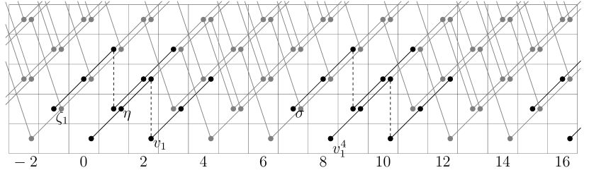
Figure 2. The spectral sequence computing the homotopy groups of $L_{K(1)}V(0)$. A $\bullet$ denotes a copy of ${{\mathbb{Z}}}/2$. Dashed vertical lines denote exotic multiplication by $2$.

Using 4.1.8 and naturality it is possible to work out the spectral sequence for the homotopy of $L_{K(1)}S^{0}$. See Figure 3. Here are the results in brief.

Proposition 4.1.9.

In the spectral sequence

$$H_{c}^{\ast}({{\mathbb{Z}}}_{2}^{\times},K_{\ast})\Longrightarrow\pi_{\ast}L_{K(1)}S^{0},$$

there are non-trivial differentials

$$d_{3}(\alpha_{4t+3}) =\eta^{3}\alpha_{4t+1}$$

$$d_{3}(\alpha_{2(2^{i}t+1)/3}) =\eta^{3}\alpha_{2^{i+1}t/i+3},\quad t\not\equiv 0\quad\mathrm{mod}\ 2$$

$$d_{3}(\alpha_{2/3}) =\eta^{3}\zeta_{1}\ .$$

The last formula can be thought of as a case of the second formula with $i=\infty$. There are additive extensions as well. In fact, by (3.1.4) we see that $\eta^{2}\alpha_{4t+1}$ must be divisible by $2$. This implies:

Corollary 4.1.10.

For any $t\in{{\mathbb{Z}}}$

$$4(2\alpha_{4t+2/3})=\eta^{2}\alpha_{4t+1}.$$

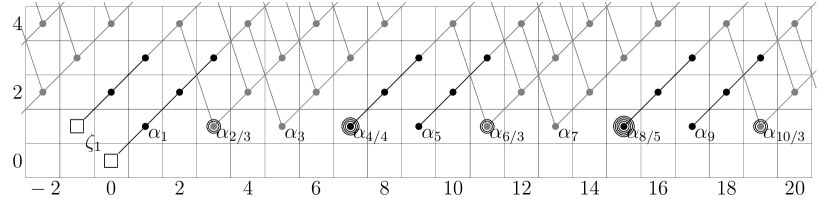
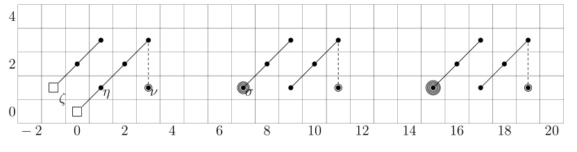
Figure 3. The $E_{2}$ (top) and $E_{\infty}$ (bottom) pages of the spectral sequence for the homotopy of $L_{K(1)}S^{0}$. Here, a $\Box$ denotes a copy of ${{\mathbb{Z}}}_{2}$, a $\bullet$ denotes a copy of ${{\mathbb{Z}}}/2$, a a copy of ${{\mathbb{Z}}}/4$ and so on. Dashed lines denote exotic multiplications by $2$.

4.1.8 has the following consequence. Recall that we are writing $\sigma$ for both the element in homotopy and the class in the $E_{2}$-term of the Adams-Novikov Spectral Sequence which detects it.

Corollary 4.1.11.

(1) In $H_{c}^{\ast}({{\mathbb{Z}}}_{2}^{\times},K_{\ast})$ we have

$$\alpha_{4/4}^{2}=0=\sigma^{2}.$$

(2) In $\pi_{\ast}L_{K(1)}S^{0}$ we have $\sigma^{2}=0$.

Proof.

For part (1), it is sufficient to prove $\alpha_{4/4}^{2}=0$ as $\sigma$ is a unit multiple of $\alpha_{4/4}$. We use that

$$H_{c}^{s}({{\mathbb{Z}}}_{2}^{\times},K_{\ast})\to H_{c}^{s}({{\mathbb{Z}}}_{2},K_{\ast}/2)$$

is an injection if $s>1$. By part (2) of 4.1.3 we have $\alpha_{4/4}\equiv v_{1}^{4}\zeta_{1}$ modulo $2$. Since $\zeta_{1}^{2}=0$, the result follows.

For part (2), we deduce from 4.1.8 that $\pi_{14}L_{K(1)}V(0)=0$. From the long exact sequence on homotopy groups, it follows that $\pi_{14}L_{K(1)}S^{0}=0$. Alternatively we could read part (2) off of Figure 3. ∎

4.1.8 is explicit about the Hopf maps $\eta$ and $\sigma$. The other Hopf map $\nu$ plays a more subtle role. See Figure 2 and Figure 3.

Proposition 4.1.12.

(1) Let $\nu\in\pi_{3}S^{0}\cong{{\mathbb{Z}}}/8$ be a generator. Then $\nu$ is non-zero in $\pi_{\ast}L_{K(1)}S^{0}$ and detected by a unit multiple of $2\alpha_{2/3}$.

(2) The class $\nu$ is non-zero in $\pi_{\ast}L_{K(1)}V(0)$ detected by $v_{1}\zeta_{1}\eta^{2}$.

(3) In $\pi_{\ast}L_{K(1)}V(0)$, $\nu$ is a multiple of $\eta$.

Proof.

From the discussion in Remark 4.1.8 we know that $\pi_{3}(L_{K(1)}S^{0})$ sits in a short exact sequence with kernel given by $E_{4}^{3,6}\cong{{\mathbb{Z}}}/2$ generated by $\eta^{3}$ and quotient given by $E_{4}^{1,4}\cong{{\mathbb{Z}}}/4$ generated by $2\alpha_{2/3}$. The result follows because of

$$4\nu=\eta^{3}\in\pi_{3}(S^{0}).$$

For the second statement, we have that $\nu\neq 0\in\pi_{\ast}L_{K(1)}V(0)$ and also that $2\alpha_{2/3}=0\in H_{c}^{\ast}({{\mathbb{Z}}}_{2}^{\times},K_{\ast}/2)$. It follows that $\nu$ must be detected by a class in filtration $s=2$ or higher and, by 4.1.8, the only class available at $E_{\infty}$ is $v_{1}\zeta_{1}\eta^{2}$.

For the third statement, we have that $\nu$ is detected by a class which is a multiple of $\eta$ in the $E_{\infty}$-page for $\pi_{\ast}L_{K(1)}V(0)$. Since there are no non-zero elements of higher filtration in the $t-s=3$ stem, the claim follows. ∎

4.2. The $K(1)$-local homotopy of the spectrum $Y$

Let $C(\eta)$ be the cone on $\eta\in\pi_{1}S^{0}$ and let $Y=V(0)\wedge C(\eta)$. The spectrum $Y$ is a type $1$ complex with a $v_{1}$-self map $v_{1}\colon\Sigma^{2}Y\to Y$. The map $v_{1}$ is not unique, but the induced map $\pi_{\ast}\Sigma^{2}L_{K(1)}Y\to\pi_{\ast}L_{K(1)}Y$ is independent of the choice. Indeed, for any $k$, $\pi_{k}L_{K(1)}Y$ is one-dimensional over ${{\mathbb{Z}}}/2$. See 4.2.2 below.

Remark 4.2.1.

By the construction of $Y$, there is a cofiber sequence

(4.2.3)

which, since $BP_{*}(V(0)\wedge\eta)=0$, gives rise to a short exact sequence of $BP_{\ast}BP$-comodules

$$0\to BP_{\ast}V(0)\to BP_{\ast}Y\to BP_{\ast}\Sigma^{2}V(0)\to 0\ .$$

This is not split, but is the non-zero element

$$\eta\in\mathrm{Ext}^{1}_{BP_{\ast}BP}(\Sigma^{2}BP_{\ast}/2,BP_{\ast}/2)\cong{{\mathbb{Z}}}/2.\$$

Proposition 4.2.2.

We have an isomorphism of $\mathbb{F}_{2}[v_{1}^{\pm 1}]$-modules

$$\mathbb{F}_{2}[v_{1}^{\pm 1}]\otimes E(\zeta_{1})\cong\mathbb{F}_{2}[v_{1}^{\pm 1}]\otimes E(\sigma)\cong H_{c}^{\ast}({{\mathbb{Z}}}_{2}^{\times},K_{\ast}Y)$$

with $v_{1}^{4}\zeta_{1}=\sigma$. The spectral sequence

$$H_{c}^{\ast}({{\mathbb{Z}}}_{2}^{\times},K_{\ast}Y)\Longrightarrow\pi_{\ast}L_{K(1)}Y$$

collapses. If $\iota\colon S^{0}\to Y$ is the inclusion of the bottom cell, then $\pi_{*}L_{K(1)}Y$ is a free module over $\mathbb{F}_{2}[v_{1}^{\pm 1}]$ on generators $\iota$ and $\iota\sigma$ of degrees $0$ and $7$ respectively.

Proof.

By Landweber exactness and 4.2.1 we have a short exact sequence of ${{\mathbb{Z}}}_{2}^{\times}$ modules

$$0\to K_{\ast}V(0)\to K_{\ast}Y\to K_{\ast}\Sigma^{2}V(0)\to 0\ .$$

Furthermore, in the long exact sequence in group cohomology, the boundary map is given by multiplication by $\eta$. The claim about $H_{c}^{\ast}({{\mathbb{Z}}}_{2}^{\times},K_{\ast}Y)$ now follows from 4.1.8. The spectral sequence for $\pi_{*}L_{K(1)}Y$ must collapse for degree reasons. ∎

Let $\iota\colon S^{0}\to Y$ and $p\colon Y\to S^{3}$ be the inclusion of the bottom cell and the collapse to the top cell of $Y$ respectively, and similarly for $\iota\colon S^{0}\to V(0)$ and $p\colon V(0)\to S^{1}$.

Proposition 4.2.3.

Let $2\colon Y\to Y$ be the degree $2$ map. Then there is a factoring

where $\nu$ is the composite After localization, the degree $2$ map

$$2\colon L_{K(1)}Y\to L_{K(1)}Y$$

is null-homotopic.

Proof.

We noted in the proof of 3.1.4 that $\pi_{\ast}V(0)$ has elements of order $4$; hence $0\neq 2:V(0)\to V(0)$. Consider the diagram

Since $S^{0}\xrightarrow{2}S^{0}\to V(0)$ is zero, the dotted factoring exists and must be non-zero. Since $\pi_{1}V(0)\cong{{\mathbb{Z}}}/2$ generated by $\eta$ we conclude there is factoring

We then have a diagram

Since $\eta=0$ in $\pi_{\ast}Y$, the dotted factoring exists and gives a factoring of $2\colon Y\to Y$ as a map

Since $K_{*}h\colon K_{\ast}Y\to K_{*}\Sigma^{2}V(0)$ is onto and $2K_{*}Y=0$, we have that $K_{*}f=0$. Since $\pi_{2}Y\to K_{2}Y$ is an injection onto the summand generated by $v_{1}$, this implies $f$ factors as a composition

The mod $2$ cohomology of $Y$ is cyclic over the Steenrod algebra and, hence, there can be no splitting

$$H^{*}(Y\wedge V(0))\cong H^{\ast}Y\oplus H^{\ast}\Sigma Y$$

as modules over the Steenrod algebra. Thus the order of the identity on $Y$ is not $2$ and we see $g\neq 0$. Finally, since $\pi_{3}Y\cong{{\mathbb{Z}}}/2$ generated by $\nu$, the first statement follows. The second statement follows as $\nu=0$ in $\pi_{\ast}L_{K(1)}Y$; indeed, we showed in 4.1.12 that $\nu$ is divisible by $\eta$ in $\pi_{\ast}L_{K(1)}V(0)$ and $Y=V(0)\wedge C(\eta)$. ∎

Recall that classes $i_{0}$ and $i_{1}$ in $\pi_{*}V(0)\wedge V(0)$ of degree $0$ and $1$ respectively were defined in 3.1.6. We abuse notation and let $i_{0}=(\jmath\wedge V(0))_{*}i_{0}$ and $i_{1}=(\jmath\wedge V(0))_{*}i_{1}$ be the corresponding classes in $\pi_{*}(Y\wedge V(0))$.

Corollary 4.2.4.

There is an equivalence

$$L_{K(1)}(Y\wedge V(0))\simeq L_{K(1)}Y\vee\Sigma L_{K(1)}Y\ .$$

Furthermore, $\pi_{*}L_{K(1)}(Y\wedge V(0))$ is a free module over $\mathbb{F}_{2}[v_{1}^{\pm 1}]\otimes E(\sigma)$ on generators $i_{0}$ and $i_{1}$ in degrees $0$ and $1$.

Proof.

This is an immediate consequence of 4.2.3. ∎

5. Height $2$ cohomology calculations

In this section we collect together some calculations of the group cohomology of $\mathbb{G}_{2}$ and many of its closed subgroups. Here we will focus on cohomology with coefficients in the Witt vectors ${{\mathbb{W}}}=W(\mathbb{F}_{4})$ and related quotient and subrings. The main result is 5.2.7 which gives a structure result for $H_{c}^{\ast}(\SS_{2}^{1},{{\mathbb{Z}}}_{2})$.

We will extend the calculations to other coefficients in the next section, when we prove 1.1.2 in the case $n=p=2$.

5.1. Preliminaries and recollections

A key to many of our calculations is the behavior and properties of the classes in $H_{c}^{1}(\mathbb{G}_{2},\mathbb{F}_{2})$; these play a central role in the story we are telling here. This is also a point where the prime $2$ has extra phenomena not seen at odd primes. The first part of this section is devoted to analyzing these cohomology classes. We will also include some material on the cohomology of some Poincaré duality subgroups of $\SS_{2}$ collected from [Bea15].

In (2.2.1) we defined the extended determinant map

$$\mathrm{det}\colon\mathbb{G}_{2}{{\longrightarrow\ }}{{\mathbb{Z}}}_{2}^{\times}\ .$$

We use it in the following definition of some key cohomological classes.

Definition 5.1.1.

Let

$$p_{1}\colon{{\mathbb{Z}}}_{2}^{\times}\to{{\mathbb{Z}}}_{2}^{\times}/\{\pm 1\}\cong{{\mathbb{Z}}}_{2}\qquad\mathrm{and}\qquad p_{2}\colon{{\mathbb{Z}}}_{2}^{\times}\to{{\mathbb{Z}}}/4^{\times}\cong\{\pm 1\}$$

be the natural projections. Using the explicit isomorphism ${{\mathbb{Z}}}_{2}^{\times}/\{\pm 1\}\cong{{\mathbb{Z}}}_{2}$ of 4.1.1, define surjective homomorphisms

(5.1.1) $${{\zeta}}_{2}:=p_{1}\circ\det\colon\mathbb{G}_{2}{{\longrightarrow\ }}{{\mathbb{Z}}}_{2}\qquad\mathrm{and}\qquad{{\chi}}_{2}:=p_{2}\circ\det\colon\mathbb{G}_{2}{{\longrightarrow\ }}{{\mathbb{Z}}}/2\ .$$

By abuse of notation, we call the corresponding cohomology classes by the same names; thus, we have classes ${{\zeta}}_{2}\in H_{c}^{1}(G,{{\mathbb{Z}}}_{2})$ and ${{\chi}}_{2}\in H_{c}^{1}(G,\mathbb{F}_{2})$ for any closed subgroup $G\subseteq\mathbb{G}_{2}$. We write ${{\zeta}}={{\zeta}}_{2}$ and ${{\chi}}={{\chi}}_{2}$ when there can be no confusion.

We will write ${{\zeta}}_{2}\in H_{c}^{1}(\mathbb{G}_{2},\mathbb{F}_{2})$ to be the reduction of ${{\zeta}}_{2}\in H_{c}^{1}(\mathbb{G}_{2},{{\mathbb{Z}}}_{2})$. We define

$${\widetilde{\chi}}\in H_{c}^{2}(\mathbb{G}_{2},{{\mathbb{Z}}}_{2})$$

to be the image of ${{\chi}}_{2}$ under the Bockstein $H_{c}^{1}(\mathbb{G}_{2},\mathbb{F}_{2})\to H_{c}^{2}(\mathbb{G}_{2},{{\mathbb{Z}}}_{2})$.

Remark 5.1.2.

The cohomology class ${{\zeta}}_{2}$ is the reduced determinant discussed earlier in (2.2.2) and (2.2.3); see also 2.2.1. The class ${{\chi}}_{2}$ is the analog of the class $\chi_{1}$ defined in 4.1.1 for $n=1$.

Looking back at 4.1.1 we see that the projections $p_{1}$ and $p_{2}$ of 5.1.1 have arisen before. In fact $p_{1}=\zeta_{1}$ and $p_{2}=\chi_{1}$, up to the isomorphism ${{\mathbb{Z}}}/4^{\times}\cong{{\mathbb{Z}}}/2$. We can write

$$\zeta_{2}=\zeta_{1}\circ\det\qquad\mathrm{and}\qquad\chi_{2}=\chi_{1}\circ\det.$$

Here are some more refined details about the behavior of $\zeta_{2}$ and $\chi_{2}$. From 2.4.6 we have decompositions $K\rtimes G_{24}\cong\SS_{2}$ and $K^{1}\rtimes G_{24}\cong\SS_{2}^{1}$. In 2.4.4, we introduced elements $\pi$ and $\alpha$ of ${{\mathbb{W}}}^{\times}\subseteq\SS_{2}$ that satisfy $\det(\pi)=3$ and $\det(\alpha)=-1$. Furthermore, $\alpha$ and $\pi$ are elements of $K\subseteq\SS_{2}$.

(1) Since $\mathrm{det}(\alpha)=-1$, it follows that ${{\chi}}_{2}(\alpha)=-1$ and ${{\zeta}}_{2}(\alpha)=0$. Thus $\alpha\in K^{1}$ and ${{\chi}}_{2}\colon\SS_{2}^{1}\to\mathbb{F}_{2}$ restricts to a non-zero class of the same name in $H_{c}^{1}(\SS_{2}^{1},\mathbb{F}_{2})$ and even in $H_{c}^{1}(K^{1},\mathbb{F}_{2})$. By definition $\SS_{2}^{1}$ is in the kernel of the reduced determinant; hence, ${{\zeta}}_{2}$ restricts to zero in $H_{c}^{1}(\SS_{2}^{1},{{\mathbb{Z}}}_{2})$.

(2) Note also that ${{\zeta}}_{2}^{2}=0$ in cohomology, wherever it appears, as it is the image of a generator of $H_{c}^{1}({{\mathbb{Z}}}_{2},{{\mathbb{Z}}}_{2})$. The exponent of ${{\chi}}_{2}$ is an important point addressed below in 5.3.1.

We now begin our calculations.

Lemma 5.1.3.

(1) The cohomology group $H_{c}^{1}(\SS_{2},\mathbb{F}_{2})$ is of dimension $2$ over $\mathbb{F}_{2}$ with basis ${{\chi}}_{2}$ and ${{\zeta}}_{2}$.

(2) The cohomology group $H_{c}^{1}(\SS_{2},{{\mathbb{Z}}}_{2})$ is free of rank one over ${{\mathbb{Z}}}_{2}$ generated by ${{\zeta}}_{2}$.

Proof.

The first statement follows from Theorem 6.3.12 of Ravenel [Rav86] by taking invariants with respect to the residual action of $\mathbb{F}_{4}^{\times}$. Alternatively, it follows from Corollary 5.4 of [Hen17] by noting that $H_{c}^{1}(\SS_{2},\mathbb{F}_{2})$ is dual to $H_{1}(\SS_{2},\mathbb{F}_{2})$ and that

$$H_{1}(\SS_{2},\mathbb{F}_{2})\cong H_{1}(S_{2},\mathbb{F}_{2})_{\mathbb{F}_{4}^{\times}}.$$

Specifically, in Proposition 5.2, we can take $c=\omega$. The class represented by $1+4\omega$ and the class represented by $1+\omega S^{2}$ are invariant for the residual action of $\mathbb{F}_{4}^{\times}$ (given by conjugation by $\omega$) while the generators $1+\omega S$, $1+\omega^{2}S$ and their product gets cyclicly permuted by $\mathbb{F}_{4}^{\times}$. The generator we call ${{\zeta}}_{2}$ is dual to the class detected by $1+4\omega$ and the generator we call ${{\chi}}_{2}$ is dual to the class detected by $1+\omega S^{2}$ in the proof of Proposition 5.2 of [Hen17].

We will see below in 5.2.9, that $0\neq{{\chi}}_{2}^{2}\in H_{c}^{2}(\SS_{2}^{1},\mathbb{F}_{2})$, and hence in $H_{c}^{2}(\SS_{2},\mathbb{F}_{2})$. The second statement then follows from examining the long exact sequence on coefficients induced by

$$0\to{{\mathbb{Z}}}_{2}\xrightarrow{2}{{\mathbb{Z}}}_{2}\to\mathbb{F}_{2}\to 0$$

and noting that the composite of the connecting homomorphism with reduction modulo $2$ (i.e., the Bockstein) is the squaring operation in cohomology. ∎

We now add some further recollections on the cohomology of the subgroups $K$ and $K^{1}$ of $\SS_{2}$. Since $\det(\pi)=3$, $\zeta_{2}(\pi)$ maps to a topological generator of ${{\mathbb{Z}}}_{2}^{\times}/\{\pm 1\}$. Then since $\pi\in K$ the composition

remains surjective and defines a non-zero cohomology class ${{\zeta}}_{2}\in H_{c}^{1}(K,{{\mathbb{Z}}}_{2})$. Any choice of splitting of this surjection will define isomorphisms $\SS_{2}^{1}\rtimes{{\mathbb{Z}}}_{2}\cong\SS_{2}$ and $K^{1}\rtimes{{\mathbb{Z}}}_{2}\cong K$. An obvious choice of a splitting sends a generator of ${{\mathbb{Z}}}_{2}$ to $\pi$.

The following can be found in Corollary 2.5.12 and Theorem 2.5.13 of [Bea15].

Lemma 5.1.4.

(1) The subgroups $K^{1}$ and $K$ are oriented Poincaré duality groups of dimensions $3$ and $4$ respectively.

(2) There is an isomorphism

$$H_{c}^{\ast}(K,\mathbb{F}_{2})\cong\mathbb{F}_{2}[{{\zeta}},{{\chi}},x_{1},x_{2}]/({{\zeta}}^{2},{{\chi}}^{2},x_{1}^{2}+{{\chi}}x_{1},x_{2}^{2}+{{\chi}}x_{2})$$

where ${{\zeta}},{{\chi}}$, $x_{1}$ and $x_{2}$ are in degree $1$.

(3) There is an isomorphism

$$H_{c}^{\ast}(K^{1},\mathbb{F}_{2})\cong\mathbb{F}_{2}[{{\chi}},x_{1},x_{2}]/({{\chi}}^{2},x_{1}^{2}+{{\chi}}x_{1},x_{2}^{2}+{{\chi}}x_{2})$$

where ${{\chi}}$, $x_{1}$ and $x_{2}$ are in degree $1$.

We also write down the cohomology of $Q_{8}\rtimes\mathbb{F}_{4}^{\times}\cong G_{24}$ and $C_{6}$. We collect these results in the following remark.

Remark 5.1.5.

Recall that $Q_{8}$ has periodic cohomology with a periodicity class $k\in H^{4}(Q_{8},{{\mathbb{Z}}}_{2})$ of order $8$. See, for example, [AM04, Ch. IV. Lemma 2.10]. We will also write $k\in H^{4}(Q_{8},\mathbb{F}_{2})$ for the reduction of $k$.

We have an isomorphism

$$\mathbb{F}_{2}[x,y,k]/(x^{2}+xy+y^{2},x^{2}y+xy^{2})\cong H^{\ast}(Q_{8},\mathbb{F}_{2})$$

where $x$ and $y$ are in degree $1$. For a choice $\omega\in\mathbb{F}_{4}$ of a primitive cube root of unity we have $\omega_{\ast}x=y$, $\omega_{\ast}y=x+y$, and $\omega_{\ast}k=k$; from this it follows that there is an isomorphism

$$\mathbb{F}_{2}[z,k]/(z^{2})\cong H^{\ast}(Q_{8},\mathbb{F}_{2})^{\mathbb{F}_{4}^{\times}}\cong H^{\ast}(G_{24},\mathbb{F}_{2})$$

where $z=x^{2}y=xy^{2}$. Finally, since $k$ has order $8$ in $H^{4}(Q_{8},{{\mathbb{Z}}}_{2})$, the Universal Coefficient Theorem gives an isomorphism

$${{\mathbb{Z}}}_{2}[k]/(8k)\cong H^{\ast}(G_{24},{{\mathbb{Z}}}_{2})\ .$$

Recall further that

$$H^{\ast}(C_{6},\mathbb{F}_{2})\cong\mathbb{F}_{2}[h]$$

for a class $h$ in degree $1$ and that

$$H^{\ast}(C_{6},{{\mathbb{Z}}}_{2})\cong{{\mathbb{Z}}}_{2}[g]/(2g)$$

for a class $g$ in degree $2$ which is the image of $h$ under the connecting homomorphism for ${{\mathbb{Z}}}_{2}\xrightarrow{2}{{\mathbb{Z}}}_{2}\to\mathbb{F}_{2}$. The inclusion $C_{6}=\{\pm 1\}\times\mathbb{F}_{4}^{\times}\subseteq G_{24}$ yields a map on cohomology

$$H^{\ast}(G_{24},{{\mathbb{Z}}}_{2})\cong{{\mathbb{Z}}}_{2}[k]/(8k)\to{{\mathbb{Z}}}_{2}[g]/(2g)\cong H^{\ast}(C_{6},{{\mathbb{Z}}}_{2})$$

sending $k$ to $g^{2}$. With $\mathbb{F}_{2}$ coefficients the map

$$H^{\ast}(G_{24},\mathbb{F}_{2})\cong\mathbb{F}_{2}[z,k]/(z^{2})\to\mathbb{F}_{2}[h]\cong H^{\ast}(C_{6},\mathbb{F}_{2})$$

sends $z$ to $0$ and $k$ to $h^{4}$.

5.2. The cohomology of $\SS_{2}^{1}$

In this section we use the algebraic duality spectral sequence of Section 2.5 to calculate the integral and mod $2$ cohomology of $\SS_{2}^{1}$ as graded modules over $H^{\ast}(G_{24},{{\mathbb{Z}}}_{2})$. From 2.5.3 we have

(5.2.1) $$\lx@xy@svg{\hbox{\raise 0.0pt\hbox{\kern 36.39523pt\hbox{\ignorespaces\ignorespaces\ignorespaces\hbox{\vtop{\kern 0.0pt\offinterlineskip\halign{\entry@#!@&&\entry@@#!@\cr&\crcr}}}\ignorespaces{\hbox{\kern-36.39523pt\raise 0.0pt\hbox{\hbox{\kern 0.0pt\raise 0.0pt\hbox{\hbox{\kern 3.0pt\raise 0.0pt\hbox{$\textstyle{E_{1}^{p,q}=H^{q}(F_{p},M)\ignorespaces\ignorespaces\ignorespaces\ignorespaces}$}}}}}}}\ignorespaces\ignorespaces\ignorespaces\ignorespaces{}{\hbox{\hbox{\kern 0.0pt\raise 1.0pt\hbox{\lx@xy@droprule}}\hbox{\kern 0.0pt\raise-1.0pt\hbox{\lx@xy@droprule}}}}\ignorespaces{\hbox{\kern 60.39523pt\raise 0.0pt\hbox{\hbox{\kern 0.0pt\raise 0.0pt\hbox{\lx@xy@tip{1.5}\lx@xy@tip{-1.5}}}}}}{\hbox{\hbox{\kern 0.0pt\raise 1.0pt\hbox{\lx@xy@droprule}}\hbox{\kern 0.0pt\raise-1.0pt\hbox{\lx@xy@droprule}}}}{\hbox{\hbox{\kern 0.0pt\raise 1.0pt\hbox{\lx@xy@droprule}}\hbox{\kern 0.0pt\raise-1.0pt\hbox{\lx@xy@droprule}}}}{\hbox{\kern 60.39523pt\raise 0.0pt\hbox{\hbox{\kern 0.0pt\raise 0.0pt\hbox{\hbox{\kern 3.0pt\raise 0.0pt\hbox{$\textstyle{H_{c}^{p+q}(\mathbb{S}_{2}^{1},M)}$}}}}}}}\ignorespaces}}}}\ignorespaces\ . \textstyle{E_{1}^{p,q}=H^{q}(F_{p},M)\ignorespaces\ignorespaces\ignorespaces\ignorespaces} \textstyle{H_{c}^{p+q}(\mathbb{S}_{2}^{1},M)} \textstyle{E_{1}^{p,q}=H^{q}(F_{p},M)\ignorespaces\ignorespaces\ignorespaces\ignorespaces} \textstyle{H_{c}^{p+q}(\mathbb{S}_{2}^{1},M)}$$

We are particularly interested in the cases $M={{\mathbb{Z}}}_{2}$ and $M=\mathbb{F}_{2}$.

This spectral sequence has a split edge homomorphism. The augmentation map ${{\mathbb{Z}}}_{2}[[\SS_{2}^{1}/G_{24}]]\to{{\mathbb{Z}}}_{2}$ induces, through the isomorphism of (2.5.1), an edge homomorphism

$$H_{c}^{\ast}(\SS_{2}^{1},{{\mathbb{Z}}}_{2})\to H^{\ast}(G_{24},{{\mathbb{Z}}}_{2})$$

of the spectral sequence (5.2.1). This is induced by the inclusion of $G_{24}\subseteq\SS_{2}^{1}$. By 2.4.6 there is a projection $\SS_{2}^{1}\to\SS_{2}^{1}/K^{1}\cong G_{24}$ which splits this inclusion, so we immediately have the following result.

Lemma 5.2.1.

Let $M={{\mathbb{Z}}}_{2}$ or $\mathbb{F}_{2}$. The map of algebras

$$H_{c}^{\ast}(\SS_{2}^{1},M)\to H^{\ast}(G_{24},M)$$

induced by the inclusion of the subgroup $G_{24}$ has an algebra splitting.

From 5.1.5 and 5.2.1 we get an injective map

$${{\mathbb{Z}}}_{2}[k]/(8k)\cong H^{\ast}(G_{24},{{\mathbb{Z}}}_{2})\to H_{c}^{\ast}(\SS_{2}^{1},{{\mathbb{Z}}}_{2}).$$

We confuse $k$ with its image in $H_{c}^{4}(\SS_{2}^{1},{{\mathbb{Z}}}_{2})$ and in the cohomology of its subgroups. An example of such a subgroup is $G^{\prime}_{24}$, the conjugate group defined in (2.4.6). Then the composition

$$H^{\ast}(G_{24},{{\mathbb{Z}}}_{2})\to H_{c}^{\ast}(\SS_{2}^{1},{{\mathbb{Z}}}_{2})\to H^{\ast}(G^{\prime}_{24},{{\mathbb{Z}}}_{2})$$

is an isomorphism; this follows from the fact that the inclusion $G^{\prime}_{24}\subseteq\SS_{2}^{1}$ also splits the projection $\SS_{2}^{1}\to G_{24}$. Also, as in 5.1.5, the map

$$H^{\ast}(G_{24},{{\mathbb{Z}}}_{2})\to H_{c}^{\ast}(\SS_{2}^{1},{{\mathbb{Z}}}_{2})\to H^{\ast}(C_{6},{{\mathbb{Z}}}_{2})\cong{{\mathbb{Z}}}_{2}[g]/(2g)$$

sends $k$ to $g^{2}$.

It will be useful to compare the algebraic duality spectral sequence for $\SS_{2}^{1}$ to a spectral sequence for a quotient group. Let $C_{2}=\{\pm 1\}\subseteq\SS_{2}$ be the central subgroup of order $2$. For any group $G\subseteq\mathbb{S}_{2}$ which contains $C_{2}$ define $PG=G/C_{2}$. Note that $C_{2}$ is a subgroup of all of the groups $\SS_{2}^{1}$, $C_{6}$, $G_{24}$, and $G_{24}^{\prime}$. Whenever $C_{2}\subseteq F$ we have isomorphisms of $\SS_{2}^{1}$-coset spaces $\SS_{2}^{1}/F\cong P\SS_{2}^{1}/PF$ and, hence isomorphisms of continuous $\SS_{2}^{1}$-modules

$${{\mathbb{Z}}}_{2}[[\SS_{2}^{1}/F]]\cong{{\mathbb{Z}}}_{2}[[P\SS_{2}^{1}/PF]]\ .$$

The resolution of 2.5.1 is in fact constructed as a resolution of continuous $P\SS_{2}^{1}$-modules

$$0\to{{\mathbb{Z}}}_{2}[[P\mathbb{S}_{2}^{1}/PF_{3}]] \mathop{{{\longrightarrow\ }}}^{\partial_{3}}{{\mathbb{Z}}}_{2}[[P\mathbb{S}_{2}^{1}/PF_{2}]]$$

(5.2.2) $$\mathop{{{\longrightarrow\ }}}^{\partial_{2}}{{\mathbb{Z}}}_{2}[[P\mathbb{S}_{2}^{1}/PF_{1}]]\mathop{{{\longrightarrow\ }}}^{\partial_{1}}{{\mathbb{Z}}}_{2}[[P\mathbb{S}_{2}^{1}/PF_{0}]]\to{{\mathbb{Z}}}_{2}\to 0\ .$$

We have

$$PF_{0} \cong A_{4}:=(C_{2}\times C_{2})\rtimes C_{3}$$

$$PF_{1} \cong PF_{2}\cong C_{3}$$

$$PF_{3} \cong A^{\prime}_{4}$$

with $A^{\prime}_{4}=\pi A_{4}\pi^{-1}$, where $\pi=1+2\omega\in{{\mathbb{W}}}^{\times}$. Note, in particular, that if $p=1$ or $2$, then ${{\mathbb{Z}}}_{2}[[P\mathbb{S}_{2}^{1}/PF_{p}]]\cong{{\mathbb{Z}}}_{2}[[P\mathbb{S}_{2}^{1}/C_{3}]]$ is a projective ${{\mathbb{Z}}}_{2}[[P\SS_{2}^{1}]]$-module. This often makes arguments with this resolution simpler. For example, if $M$ is a profinite $P\SS_{2}^{1}$ module we have an analog of the algebraic duality spectral sequence

$$H^{q}(PF_{p},M)\Longrightarrow H_{c}^{p+q}(P\mathbb{S}_{2}^{1},M)$$

with

(5.2.3) $$E_{1}^{p,q}=H^{q}(C_{3},M)=0$$

if $p=1$, $2$ and $q>0$.

Finally, these considerations give a diagram of spectral sequences for any profinite $P\SS_{2}^{1}$-module $M$

with the vertical maps are induced by the evident quotient homomorphisms.

Lemma 5.2.2.

Let $M={{\mathbb{Z}}}_{2}$ or $\mathbb{F}_{2}$. The spectral sequence

collapses at the $E_{2}$-page. Furthermore, if $M=\mathbb{F}_{2}$, it collapses at the $E_{1}$-page.

Proof.

Since $H^{q}(PF_{p},M)=0$ for $p=1,2$ and $q>0$, and since $H^{\ast}(PF_{0},M)$ is a retract of $H_{c}^{\ast}(P\SS_{2}^{1},M)$, the spectral sequence collapses at $E_{2}$. The $d_{1}$-differential is induced by the maps $\partial_{i}$ of 2.5.1. By part (2) of 2.5.1 we have that $d_{1}\equiv 0$ modulo $2$, so the spectral sequence collapses at $E_{1}$ for $M=\mathbb{F}_{2}$. ∎

It is also useful to compare these spectral sequences to yet another one defined for a subgroup of $\SS_{2}^{1}$. Recall there is a semidirect product decomposition $\SS_{2}^{1}\cong K^{1}\rtimes G_{24}$; this implies a decomposition $P\SS_{2}^{1}\cong K^{1}\rtimes A_{4}$. Thus, the resolution (5.2) is a resolution of projective ${{\mathbb{Z}}}_{2}[[K^{1}]]$-modules. For any profinite $P\SS_{2}^{1}$-module $M$, we get a diagram of spectral sequences

(5.2.4)

and in the bottom row the $\mathrm{Ext}$ groups vanish if $q>0$. This allows us to prove the following lemma. Note that part (1) of 5.1.4 implies $H_{c}^{3}(K^{1},M)\cong M$ for $M$ either ${{\mathbb{Z}}}_{2}$ or $\mathbb{F}_{2}$.

Lemma 5.2.3.

Let $M={{\mathbb{Z}}}_{2}$ or $\mathbb{F}_{2}$. The sequence

is split short exact, where the maps are induced by the projection to $A_{4}$ and the inclusion of $K^{1}$ in $P\SS_{2}^{1}\cong K^{1}\rtimes A_{4}$. Furthermore the restriction homomorphism

$$H_{c}^{3}(\SS_{2}^{1},M)\longrightarrow H_{c}^{3}(K^{1},M)$$

is split surjective.

Proof.

The second statement follows from the first since the map $H_{c}^{3}(P\SS_{2}^{1},M)\to H_{c}^{3}(K^{1},M)$ factors through $H_{c}^{3}(\SS_{2}^{1},M)\to H_{c}^{3}(K^{1},M)$.

For the first statement, we use the map of spectral sequences (5.2.4). Since ${{\mathbb{Z}}}_{2}[[P\SS_{2}^{1}/A^{\prime}_{4}]]\cong{{\mathbb{Z}}}_{2}[[K^{1}]]$ as a $K^{1}$-module, $\mathop{\mathrm{Hom}}\nolimits_{{{\mathbb{Z}}}_{2}[[K^{1}]]}({{\mathbb{Z}}}_{2}[[P\SS_{2}^{1}/A^{\prime}_{4}]],M)\cong M$ and, at $E_{1}^{3,0}$, the map (5.2.4) is the inclusion of the invariants

$$M^{A^{\prime}_{4}}\cong\mathop{\mathrm{Hom}}\nolimits_{{{\mathbb{Z}}}_{2}[[P\SS_{2}^{1}]]}({{\mathbb{Z}}}_{2}[[P\SS_{2}^{1}/A^{\prime}_{4}]],M)\to\mathop{\mathrm{Hom}}\nolimits_{{{\mathbb{Z}}}_{2}[[K^{1}]]}({{\mathbb{Z}}}_{2}[[P\SS_{2}^{1}/A^{\prime}_{4}]],M)\cong M.$$

The action of $A_{4}^{\prime}$ on $M$ is trivial, so this is an isomorphism.

By part (2) of 2.5.1, $E_{2}^{3,0}\cong E_{1}^{3,0}$ for both $K^{1}$ and $P\SS_{2}^{1}$ as the differential $d_{1}\colon E_{1}^{2,0}\to E_{1}^{3,0}$ is induced by the map $\partial_{3}$, which is zero modulo $IK^{1}$. Both spectral sequences collapse at the $E_{2}$-term. For $K^{1}$ this follows for degree reasons and for $P\SS_{2}^{1}$, this is 5.2.2. So the map in (5.2.4) at $E_{\infty}^{3,0}$ is an isomorphism. Finally, for $P\SS_{2}^{1}$ we have $E_{\infty}^{2,1}=E_{\infty}^{1,2}=0$ by (5.2.3). Since $E_{\infty}^{0,3}\cong H^{3}(PF_{0},M)$ is a retract of $H_{c}^{3}(P\SS_{2}^{1},M)$, the extension is split. ∎

Remark 5.2.4.

In results to follow we will use extra structure on the algebraic duality spectral sequence. For all profinite $\SS_{2}^{1}$-modules $M$, there is a natural action of

$$\mathrm{Ext}^{\ast}_{{{\mathbb{Z}}}_{2}[[\SS_{2}^{1}]]}({{\mathbb{Z}}}_{2},{{\mathbb{Z}}}_{2})\cong H_{c}^{\ast}(\SS_{2}^{1},{{\mathbb{Z}}}_{2})$$

on $\mathrm{Ext}^{\ast}_{{{\mathbb{Z}}}_{2}[[\SS_{2}^{1}]]}(M,{{\mathbb{Z}}}_{2})$ so, in particular, the algebraic duality spectral sequence

$$H^{q}(F_{p},{{\mathbb{Z}}}_{2})\Longrightarrow H_{c}^{p+q}(\SS_{2}^{1},{{\mathbb{Z}}}_{2})$$

is a spectral sequence of $H_{c}^{\ast}(\SS_{2}^{1},{{\mathbb{Z}}}_{2})$-modules. Furthermore, the action of $H_{c}^{\ast}(\SS_{2}^{1},{{\mathbb{Z}}}_{2})$ on $E_{1}^{p,\ast}\cong H^{\ast}(F_{p},{{\mathbb{Z}}}_{2})$ is through the restriction homomorphism induced by the inclusion $F_{p}\subseteq\SS_{2}^{1}$.

We go into more detail on this algebra action in Section 8.1; see the material after Lemma 8.1.1.

Remark 5.2.5.

We are now ready to use the algebraic duality spectral sequence to compute the cohomology of $\SS_{2}^{1}$ with ${{\mathbb{Z}}}_{2}$ and $\mathbb{F}_{2}$ coefficients. In arguments below we may use the notation $E_{r}^{\ast,\ast}(\mathbb{F}_{2})$ or $E_{r}^{\ast,\ast}({{\mathbb{Z}}}_{2})$ for the algebraic duality spectral sequences converging to $H_{c}^{\ast}(\SS_{2}^{1},\mathbb{F}_{2})$ or $H_{c}^{\ast}(\SS_{2}^{1},{{\mathbb{Z}}}_{2})$ respectively.

Figure 4 displays the $E_{1}$-term with $\mathbb{F}_{2}$-coefficients in the left column, the $E_{1}$-term with ${{\mathbb{Z}}}_{2}$-coefficients in the middle column, and the $E_{\infty}$-term with ${{\mathbb{Z}}}_{2}$-coefficients in the right column. We will have $E_{1}=E_{\infty}$ for $\mathbb{F}_{2}$-coefficients. See 5.2.8.

We explain the notation in this figure; let $M=\mathbb{F}_{2}$ or ${{\mathbb{Z}}}_{2}$. Then a vertical subcolumn in an $E_{1}$-term displays a copy of $H^{\ast}(F_{p},M)$ where $F_{p}=G_{24}$ if $p=0$, $C_{6}$ if $p=1$ or $2$, or $G^{\prime}_{24}$ if $p=3$. The cohomology rings of $G_{24}$ and $C_{6}$ were discussed in 5.1.5. The symbol denotes a copy of ${{\mathbb{Z}}}/8$, while a $\bullet$ denotes a copy of ${{\mathbb{Z}}}/2$. A $\square$ denotes a copy of ${{\mathbb{Z}}}_{2}$.

We write $\Delta_{0}\in H^{0}(F_{0},M)$, $b_{0}\in H^{0}(F_{1},M)$, $\overline{b}_{0}\in H^{0}(F_{2},M)$, $\overline{\Delta}_{0}\in H^{0}(F_{3},M)$ for the generators corresponding to the ring units. This notation is used to facilitate references to [Bea17b]. Thus, for example, $E^{1,\ast}_{1}\cong H^{\ast}(C_{6},M)b_{0}$ as a module over $H_{c}^{\ast}(\SS_{2}^{1},M)$.

The generators of $\Delta_{0}$, $b_{0}$, $\overline{b}_{0}$, and $\overline{\Delta}_{0}$ are, strictly speaking, each an element of $H^{0}(F_{p},M)$ for some $p$. In the next few results, when elements survive to the $E_{2}$-term, we will conflate them with their images under the edge homomorphism

$$E_{2}^{p,0}\longrightarrow E_{\infty}^{p,0}\subseteq H_{c}^{p}(\SS_{2}^{1},M)$$

of the algebraic duality spectral sequence.

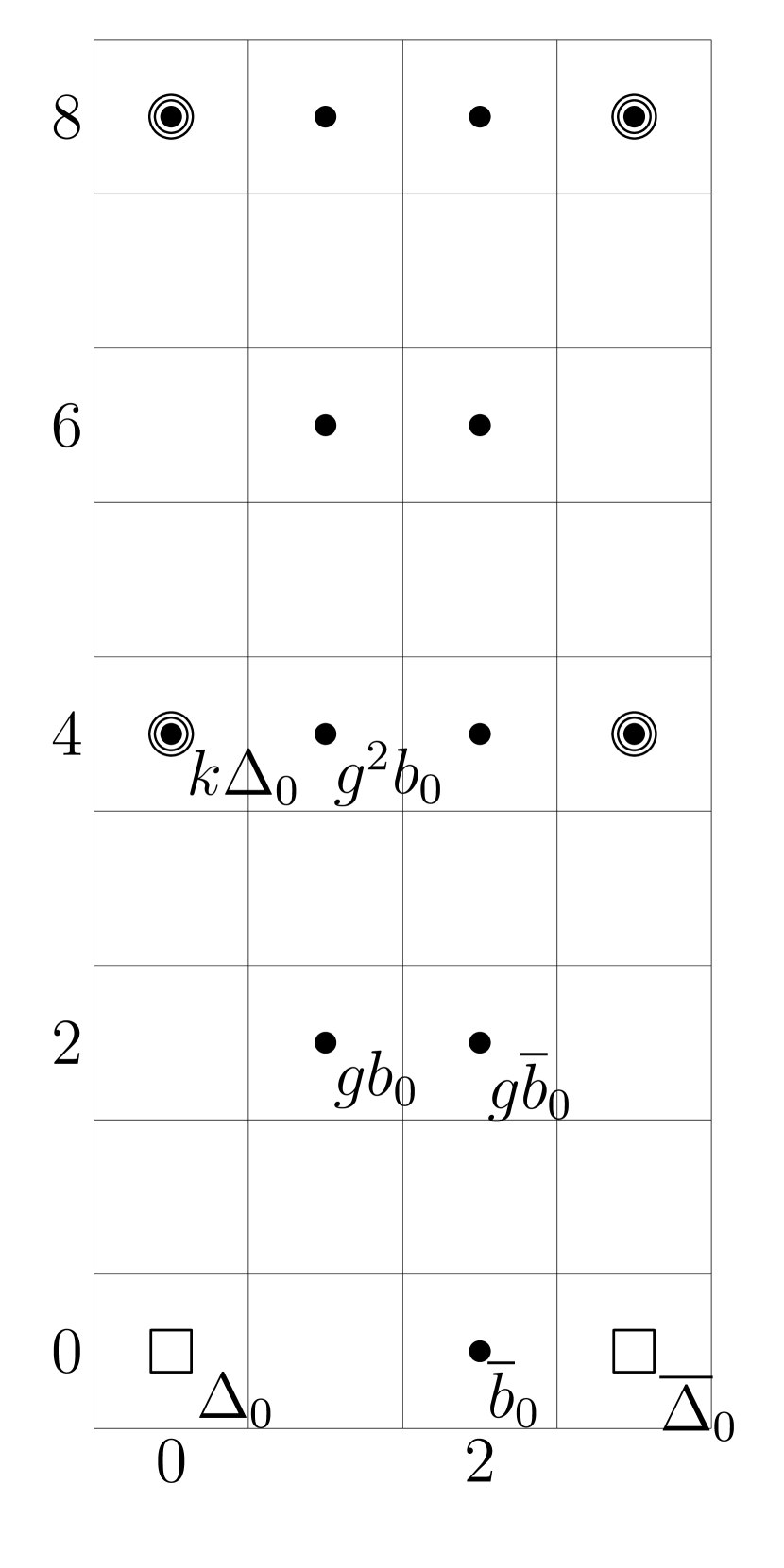
Figure 4. The $E_{1}=E_{\infty}$-term (left) of the ADSS for $H_{c}^{*}(\mathbb{S}_{2}^{1},\mathbb{F}_{2})$ and the $E_{1}$-term (center) and $E_{2}=E_{\infty}$-term (right) of the ADSS for $H_{c}^{*}(\mathbb{S}_{2}^{1},{{\mathbb{Z}}}_{2})$.

Before getting to our main theorems, we give some preliminary results about the classes $b_{0}$, $\overline{b}_{0}$, and $\overline{\Delta}_{0}$ in $E_{1}^{\ast,0}$ for both $\mathbb{F}_{2}$ and ${{\mathbb{Z}}}_{2}$. Recall from 5.1.1 that ${\widetilde{\chi}}\in H_{c}^{2}(\mathbb{G}_{2},{{\mathbb{Z}}}_{2})$ is the Bockstein on ${{\chi}}={{\chi}}_{2}\in H_{c}^{1}(\mathbb{G}_{2},\mathbb{F}_{2})$.

Lemma 5.2.6.

(1) The class $b_{0}\in E_{1}^{1,0}(\mathbb{F}_{2})$ detects ${{\chi}}\in H_{c}^{1}(\SS_{2}^{1},\mathbb{F}_{2})$.

(2) The class $\overline{b}_{0}\in E_{1}^{2,0}(\mathbb{F}_{2})$ detects ${{\chi}}^{2}\in H_{c}^{2}(\SS_{2}^{1},\mathbb{F}_{2})$, and the class $\overline{b}_{0}\in E_{1}^{2,0}({{\mathbb{Z}}}_{2})$ detects the class ${\widetilde{\chi}}\in H_{c}^{2}(\SS_{2}^{1},{{\mathbb{Z}}}_{2})$.

(3) There is a torsion-free class $e\in H_{c}^{3}(\SS_{2}^{1},{{\mathbb{Z}}}_{2})$ detected by $\overline{\Delta}_{0}\in E_{2}^{3,0}({{\mathbb{Z}}}_{2})$ which restricts to a generator of

$$H_{c}^{3}(K^{1},{{\mathbb{Z}}}_{2})\cong{{\mathbb{Z}}}_{2}.$$

Proof.

For part (1) we see that in the spectral sequence for $H_{c}^{\ast}(\SS_{2}^{1},\mathbb{F}_{2})$ (the left-hand column in Figure 4) we have $E_{\infty}^{1,0}(\mathbb{F}_{2})=\mathbb{F}_{2}$ generated by $b_{0}$ and $E_{\infty}^{0,1}=0$; hence $H_{c}^{1}(\SS_{2}^{1},\mathbb{F}_{2})\cong\mathbb{F}_{2}$. Since ${{\chi}}\in H_{c}^{1}(\SS_{2}^{1},\mathbb{F}_{2})$ is not zero, it must be detected by $b_{0}$.

For part (2) we recall from part (2) of 2.5.1 that in the integral spectral sequence (the central column in Figure 4)

$$d_{1}\colon E_{1}^{1,0}({{\mathbb{Z}}}_{2})\to E_{1}^{2,0}({{\mathbb{Z}}}_{2})$$

is multiplication by $2$. Indeed, we are working $2$-locally, $\partial_{1}\equiv 2$ modulo $(8,IS_{2}^{1})$ and the action of $IS_{2}^{1}$ on ${{\mathbb{Z}}}_{2}$ is trivial. Thus $H_{c}^{2}(\SS_{2}^{1},{{\mathbb{Z}}}_{2})\cong{{\mathbb{Z}}}/2$ generated by a class detected by $\overline{b}_{0}$. This implies that the connecting homomorphism $H_{c}^{1}(\SS_{2}^{1},\mathbb{F}_{2})\to H_{c}^{2}(\SS_{2}^{1},{{\mathbb{Z}}}_{2})$ must be non-zero. Since $H_{c}^{1}(\SS_{2}^{1},\mathbb{F}_{2})\cong\mathbb{F}_{2}$ generated by ${{\chi}}$, we must have that the generator of $H_{c}^{2}(\SS_{2}^{1},{{\mathbb{Z}}}_{2})$ is ${\widetilde{\chi}}$. From this it follows that $\overline{b}_{0}$ detects ${{\chi}}^{2}\in H_{c}^{2}(\SS_{2}^{1},\mathbb{F}_{2})$.

This leaves part (3). The integral algebraic duality spectral sequence has an edge homomorphism

$${{\mathbb{Z}}}_{2}\cong\mathop{\mathrm{Hom}}\nolimits_{{{\mathbb{Z}}}_{2}[[\SS_{2}^{1}]]}({{\mathbb{Z}}}_{2}[[\SS_{2}^{1}/G^{\prime}_{24}]],{{\mathbb{Z}}}_{2})=E_{1}^{3,0}\to H_{c}^{3}(\SS_{2}^{1},{{\mathbb{Z}}}_{2}).$$

This map is injective. To see this, note that $\overline{b}_{0}$ is a permanent cycle. Thus, the differential $d_{1}\colon E_{1}^{2,0}\to E_{1}^{3,0}$ is zero. All other differentials with target $E_{r}^{3,0}$ have zero source.

Let $e$ be the image of $\overline{\Delta}_{0}$. That $e$ restricts to a generator of $H_{c}^{3}(K^{1},{{\mathbb{Z}}}_{2})$ follows from 5.2.3. ∎

We can now give the calculation of $H_{c}^{\ast}(\SS_{2}^{1},{{\mathbb{Z}}}_{2})$ as a module over $H^{\ast}(G_{24},{{\mathbb{Z}}}_{2})$. We give the integral calculation first as there are fewer possible differentials. Some of the generators in this result are written as products; this is meant only to be evocative of their antecedents in the spectral sequence. Thus, for example, $g{{\chi}}$ is not a product in the cohomology ring $H_{c}^{\ast}(\SS_{2}^{1},{{\mathbb{Z}}}_{2})$, but a class detected by $gb_{0}$.

Theorem 5.2.7.

As an $H^{\ast}(G_{24},{{\mathbb{Z}}}_{2})\cong{{\mathbb{Z}}}_{2}[k]/(8k)$-module $H_{c}^{\ast}(\SS_{2}^{1},{{\mathbb{Z}}}_{2})$ is generated by elements

$$1,\ g{{\chi}},\ g^{2}{{\chi}},\ {\widetilde{\chi}},\ g{\widetilde{\chi}},\ e$$

of degrees $0$, $3$, $5$, $2$, $4$, and $3$ respectively and subject only to the relations

$$2g{{\chi}}=2g^{2}{{\chi}}=2{\widetilde{\chi}}=2g{\widetilde{\chi}}=0.$$

Proof.

As a reminder, we are using the algebraic duality spectral sequence of 2.5.3 with $M={{\mathbb{Z}}}_{2}$. The $E_{1}$-page is determined as an $H^{\ast}(G_{24},{{\mathbb{Z}}}_{2})$-module by 5.1.5 and the result is displayed in the center column of Figure 4. Then 2.5.1 part (2) implies that $0=d_{1}\colon E_{1}^{p,\ast}\to E_{1}^{p+1,\ast}$ if $p=0$ or $p=2$ and the same result implies

$$d_{1}\colon E_{1}^{1,q}\to E_{1}^{2,q}$$

is multiplication by $2$ and, hence, non-zero only if $q=0$. From $E_{2}$ onwards, the spectral sequence is too sparse for differentials. The result will now follow if we can show that there are no extensions.

Because we have a spectral sequence of modules over $H_{c}^{\ast}(\SS_{2}^{1},{{\mathbb{Z}}}_{2})$, as in 5.2.4, by 5.2.1 we also have a spectral sequence of $H^{\ast}(G_{24},{{\mathbb{Z}}}_{2})$-modules. By periodicity with respect to $k$, we need only check that the extensions

$$0\to{{\mathbb{Z}}}_{2}\cong E_{\infty}^{3,0}\to H_{c}^{3}(\SS_{2}^{1},{{\mathbb{Z}}}_{2})\to E_{\infty}^{1,2}\cong\mathbb{F}_{2}\to 0$$

and

$$0\to{{\mathbb{Z}}}/2\cong E_{\infty}^{2,2}\to H_{c}^{4}(\SS_{2}^{1},{{\mathbb{Z}}}_{2})\to E_{\infty}^{0,4}\cong{{\mathbb{Z}}}/8\to 0$$

are split. That the first is split follows from the second statement of 5.2.6 with $M={{\mathbb{Z}}}_{2}$. That the second is split follows from 5.2.1. ∎

We now turn to the calculation of $H_{c}^{\ast}(\SS_{2}^{1},\mathbb{F}_{2})$, again using the algebraic duality spectral sequence of 2.5.3 with $M=\mathbb{F}_{2}$. The result is displayed in the left column of Figure 4.

As is 5.1.5, write $H^{\ast}(G_{24},\mathbb{F}_{2})\cong\mathbb{F}_{2}[z,k]/(z^{2})$ and $H^{\ast}(C_{6},\mathbb{F}_{2})\cong\mathbb{F}_{2}[h]$. The class $k\in H^{4}(G_{24},{{\mathbb{Z}}}_{2})$ reduces to the class of the same name in $H^{4}(G_{24},\mathbb{F}_{2})$ and the class $g\in H^{2}(C_{6},{{\mathbb{Z}}}_{2})$ reduces to $h^{2}\in H^{2}(C_{6},\mathbb{F}_{2})$.

Corollary 5.2.8.

The algebraic duality spectral sequence for $H_{c}^{\ast}(\SS_{2}^{1},\mathbb{F}_{2})$ collapses at $E_{1}$. As a module over $\mathbb{F}_{2}[k]$, $H_{c}^{\ast}(\SS_{2}^{1},\mathbb{F}_{2})$ is freely generated by classes

$$1,\ z,\ e,\ ze,\ h^{i}{{\chi}},\ h^{i}{{\chi}}^{2}$$

with $0\leq i\leq 3$. These classes are of degrees $0$, $3$, $3$, $6$, $1+i$, $2+i$ respectively.

Proof.

The $E_{1}$-page of the spectral sequence is displayed in the left column of Figure 4. That this spectral sequence collapses follows from 5.2.1, the Universal Coefficient Theorem and 5.2.7. ∎

A key input for our main result on the homotopy type of $L_{K(1)}L_{K(2)}S^{0}$ is the exact nilpotence order of the class ${{\chi}}={{\chi}}_{2}\in H_{c}^{1}(\mathbb{G}_{2},\mathbb{F}_{2})$. The following is a preliminary step. The final result is below in 5.3.1.

Proposition 5.2.9.

Let ${{\chi}}\in H_{c}^{1}(\SS_{2}^{1},\mathbb{F}_{2})$ be the restriction of ${{\chi}}\in H_{c}^{1}(\mathbb{G}_{2},\mathbb{F}_{2})$. Then ${{\chi}}^{2}\neq 0$ and ${{\chi}}^{3}=0$ in $H_{c}^{\ast}(\SS_{2}^{1},\mathbb{F}_{2})$.

Proof.

We already have ${{\chi}}^{2}\neq 0$, by 5.2.8, so we need to show ${{\chi}}^{3}=0$. The homomorphism ${{\chi}}\colon\SS_{2}^{1}\to\mathbb{F}_{2}$ is trivial on the central element $-1\in\SS_{2}$, hence it comes from a unique class $b\in H_{c}^{1}(P\SS_{2}^{1},\mathbb{F}_{2})$. This class restricts to zero in $H^{1}(A_{4},\mathbb{F}_{2})$. We will show that $b^{3}=0$.

To see this, recall the decomposition $P\SS_{2}^{1}=K^{1}\rtimes A_{4}$. 5.2.3 implies that the map

$$H_{c}^{3}(P\SS_{2}^{1},\mathbb{F}_{2})\to H_{c}^{3}(K^{1},\mathbb{F}_{2})\times H^{3}(A_{4},\mathbb{F}_{2})$$

defined by the two restriction maps is an isomorphism. Then, from part (3) of 5.1.4, and the fact that ${{\chi}}$ (and hence $b$) restricts to the class with the same name in $H_{c}^{1}(K^{1},\mathbb{F}_{2})$, we have that $b^{3}$ restricts to $0$ in $H_{c}^{3}(K^{1},\mathbb{F}_{2})$. Since $b$ restricts to $0$ in $H^{1}(A_{4},\mathbb{F}_{2})$, the result follows. ∎

5.3. The exponent of ${{\chi}}_{2}$ in the cohomology of $\SS_{2}$

We next turn to the analysis of the cohomology of $\SS_{2}$ itself. It is natural to ask for a complete calculation of $H_{c}^{\ast}(\SS_{2},\mathbb{F}_{2})$; however, at this point, we have no succinct story to tell, and we won’t need this calculation in later sections, so we won’t follow this idea here. Some of the difficulty arises because we do not have an algebraic duality spectral sequence for $\SS_{2}$. For this reason, to prove the next result we will examine the Lyndon-Hochschild-Serre Spectral Sequence (LHSSS) for the split group extension $K\to\SS_{2}\to G_{24}$ of 2.4.6.

Proposition 5.3.1.

In $H_{c}^{\ast}(\SS_{2},\mathbb{F}_{2})$, the class ${{\chi}}={{\chi}}_{2}\in H_{c}^{1}(\SS_{2},\mathbb{F}_{2})$ has nilpotence order exactly 3; that is, ${{\chi}}^{2}\neq 0$ and ${{\chi}}^{3}=0$.

Proof.

We write $H^{\ast}(G)=H_{c}^{\ast}(G,\mathbb{F}_{2})$ in this argument. Recall from 5.2.9 that ${{\chi}}$ maps to the like-named class ${{\chi}}\in H^{1}(\SS_{2}^{1})$ and there we have ${{\chi}}^{2}\neq 0$ and ${{\chi}}^{3}=0$. It follows immediately that ${{\chi}}^{2}\neq 0$ in $H^{2}(\SS_{2})$. It remains to show ${{\chi}}^{3}=0$ in $H^{\ast}(\SS_{2})$.

We will use that ${{\chi}}^{3}$ restricts to zero in $H^{\ast}(\SS^{1}_{2})$ and a comparison of Lyndon-Hochschild-Serre Spectral Sequences induced by the inclusion $i\colon\SS_{2}^{1}\to\SS_{2}$:

(5.3.1)

From 5.1.4 we have a decomposition $H^{\ast}(K)\cong H^{\ast}(K^{1})\otimes E({{\zeta}})$. Since ${{\zeta}}$ lifts to $H^{\ast}(\mathbb{G}_{2})$, it is necessarily $G_{24}$-invariant; hence, this is an isomorphism of $G_{24}$-algebras and we have an isomorphism

$$H^{\ast}(G_{24},H^{\ast}(K))\cong H^{\ast}(G_{24},H^{\ast}(K^{1}))\otimes E({{\zeta}})\ .$$

Note that ${{\zeta}}\in E_{2}^{0,1}\cong H^{0}(G_{24},H^{1}(K))$; therefore, we can deduce an isomorphism

(5.3.2) $$E_{2}^{p,q}\cong H^{p}(G_{24},H^{q}(K))\cong H^{p}(G_{24},H^{q}(K^{1}))\oplus H^{p}(G_{24},H^{q-1}(K^{1})){{\zeta}}\ .$$

The map $i^{\ast}$ of $E_{2}$ terms in (5.3.1) is the algebra map sending ${{\zeta}}$ to zero. The class ${{\chi}}$ is detected in $E_{2}^{0,1}\cong H^{0}(G_{24},H^{1}(K))$.

As with any spectral sequence, the LHSSS gives a filtration

$$F^{3,0}\subseteq F^{2,1}\subseteq F^{1,2}\subseteq F^{0,3}=H^{3}(\SS_{2})$$

with

$$E_{\infty}^{p,q}=F^{p,q}/F^{p+1,q-1}$$

a subquotient of $E_{2}^{p,q}\cong H^{p}(G_{24},H^{q}(K))$. There is a similar filtration for $H^{2}(\SS_{2})$.

We will show that ${{\chi}}^{3}\in F^{3,0}$ and hence it is in the image of the map $H^{\ast}(G_{24})\to H^{\ast}(\SS_{2})$ induced by the projection $\SS_{2}\to G_{24}$. Since this map has a section by 5.2.1 and $\chi$ restricts to $0$ in $H^{1}(G_{24})=0$, we will have ${{\chi}}^{3}=0$ in $H^{\ast}(\SS_{2})$.

Since ${{\chi}}^{2}=0$ in $H^{2}(K)$ we have ${{\chi}}^{2}\in F^{1,1}$. Thus ${{\chi}}^{2}$ is detected by a permanent cycle

$${{\gamma}}\in H^{1}(G_{24},H^{1}(K))\ .$$

It follows that the class ${{\chi}}^{3}$ is detected at $E_{\infty}^{1,2}$ by the class ${{\chi}}{{\gamma}}$.

By 5.1.5 we know $H^{1}(G_{24})=H^{2}(G_{24})=0$. Then (5.3.2) forces the map

$$i^{\ast}\colon H^{p}(G_{24},H^{1}(K))\to H^{p}(G_{24},H^{1}(K^{1}))$$

at the $E_{2}^{p,1}$-term to be an isomorphism for $p=1,2$; in particular, if ${{\chi}}{{\gamma}}\neq 0$ in $H^{1}(G_{24},H^{2}(K))$ then $i^{\ast}({{\chi}}{{\gamma}})={{\chi}}i^{\ast}({{\gamma}})\neq 0$ in $H^{1}(G_{24},H^{2}(K^{1}))$. But ${{\chi}}^{3}=0$ in $H^{\ast}(\SS_{2}^{1})$, so we have ${{\chi}}{{\gamma}}=0$ and we can conclude ${{\chi}}^{3}\in F^{2,1}$.

Let ${{\chi}}^{3}\in H^{\ast}(\SS_{2})$ be detected by a permanent cycle ${{\varepsilon}}$ in $H^{2}(G_{24},H^{1}(K))$. Since ${{\chi}}^{3}=0$ in $H^{\ast}(\SS_{2}^{1})$ and $i^{*}$ is an isomorphism at $E_{2}^{2,1}$, we have an equation $d_{2}({{\omega}})=i^{\ast}({{\varepsilon}})$ in the LHSSS for $H^{\ast}(\SS_{2}^{1})$. Since the map $i^{\ast}$ of $E_{2}$-terms in (5.3.1) is a surjection, this implies ${{\varepsilon}}$ itself is in the image of $d_{2}$. Thus ${{\chi}}^{3}\in F^{3,0}$ as needed. ∎

6. The cohomology of $H_{c}^{\ast}(\mathbb{G}_{2},E_{0})$

We now come to one of the key results of the paper: we show the inclusion of ${{\mathbb{W}}}\to E_{0}\cong{{\mathbb{W}}}[[u_{1}]]$ of continuous $G$-modules yields an isomorphism

See 6.1.4 below. This verifies the Chromatic Vanishing Conjecture (see 1.1.2) in the case $n=p=2$. It is also a remarkable simplification and at the heart of much of what we can prove in $K(2)$-local homotopy theory. At the end of the section we give some related rational calculations.

6.1. Chromatic vanishing at $n=p=2$

We begin with the following basic case, which gives a tight control over the algebraic duality spectral sequence of 2.5.3 for $M=E_{0}/2$. As in 5.2.5 and 5.2.6 we write $\Delta_{0}$, $b_{0}$, $\overline{b}_{0}$, and $\overline{\Delta}_{0}$ for the obvious generator of $H^{0}(F_{p},\mathbb{F}_{2})$, for $p=0$ through $3$ respectively. This gives generators in $H^{0}(F_{p},E_{0}/2)$ as well.

Theorem 6.1.1.

Let $i\colon\mathbb{F}_{4}\to E_{0}/2\cong\mathbb{F}_{4}[[u_{1}]]$ be the inclusion of the constants. Then the induced map of algebraic duality spectral sequences

(6.1.1)

becomes an isomorphism at $E_{2}$ and yields an isomorphism

$$i_{\ast}\colon H_{c}^{*}(\mathbb{S}_{2}^{1},\mathbb{F}_{4})\xrightarrow{\cong}H_{c}^{*}(\mathbb{S}_{2}^{1},E_{0}/2).$$

Proof.

We first show that the map is one-to-one. Recall from 2.4.1 that $v_{1}=u^{-1}u_{1}$ for our formal group. This is a $\mathbb{G}_{2}$-invariant element modulo $2$; hence the quotient map

$$E_{\ast}/2\longrightarrow E_{\ast}/(2,v_{1})\cong\mathbb{F}_{4}[u^{\pm 1}]$$

is $\mathbb{G}_{2}$-equivariant. The composite map

$$H_{c}^{*}(\mathbb{S}_{2}^{1},\mathbb{F}_{4})\to H_{c}^{*}(\mathbb{S}_{2}^{1},E_{0}/2)\to H_{c}^{*}(\mathbb{S}_{2}^{1},E_{0}/(2,u_{1}))$$

is then an isomorphism because it is induced by the isomorphism $\mathbb{F}_{4}\cong E_{0}/(2,u_{1})$ on coefficients. For similar reasons the map on $E_{1}$-terms of (6.1.1) must also be an injection.

The hard part is to show that the map induced by $i$ is surjective on the $E_{2}$-term. Here we need Theorem 1.2.2 of [Bea17b]. From there we read that the $E_{2}=E_{\infty}$-term of the algebraic duality spectral sequence for $E_{0}/2$ is free over $\mathbb{F}_{4}[k]$ on elements

$$\Delta_{0} \in H^{0}(F_{0},E_{0}/2)$$

$$\nu^{2}y\Delta_{-1} \in H^{3}(F_{0},E_{0}/2)$$

$$h^{i}b_{0} \in H^{i}(F_{1},E_{0}/2),\qquad 0\leq i\leq 3,$$

$$h^{i}\overline{b}_{0} \in H^{i}(F_{2},E_{0}/2),\qquad 0\leq i\leq 3,$$

$$\overline{\Delta}_{0} \in H^{0}(F_{3},E_{0}/2)$$

$$\nu^{2}y\overline{\Delta}_{-1} \in H^{3}(F_{3},E_{0}/2)\ .$$

(Here, the elements $\Delta_{0},b_{0},\overline{b}_{0},\overline{\Delta}_{0}$ are the images of the same named generators from 5.2.5 under the natural maps $H^{0}(F_{p},\mathbb{F}_{2})\to H^{0}(F_{p},E_{0}/2)$.) This, the left column of Figure 4, and 5.2.8 imply that on the $E_{2}$-pages of spectral sequences (6.1.1) $i_{\ast}$ induces an injective homomorphism of free graded $\mathbb{F}_{4}[k]$-modules with the same number of generators in each bidegree. Thus our map must be onto. ∎

We can now give an integral statement. By 2.2.2 there is an isomorphism

(6.1.2) $${{\mathbb{W}}}\otimes_{{{\mathbb{Z}}}_{2}}H_{c}^{\ast}(\SS_{2}^{1},{{\mathbb{Z}}}_{2})\cong H_{c}^{\ast}(\SS_{2}^{1},{{\mathbb{W}}}).$$

Hence 5.2.7 gives an explicit computation of $H_{c}^{\ast}(\SS_{2}^{1},{{\mathbb{W}}})$ using the algebraic duality spectral sequence.

Corollary 6.1.2.

Let $i\colon{{\mathbb{W}}}\to E_{0}\cong{{\mathbb{W}}}[[u_{1}]]$ be the inclusion of the constants. Then $i$ induces an isomorphism

$$H_{c}^{*}(\mathbb{S}_{2}^{1},\mathbb{W})\cong H_{c}^{*}(\mathbb{S}_{2}^{1},E_{0}).$$

Proof.

That $i$ induces an isomorphism

$$H_{c}^{*}(\mathbb{S}_{2}^{1},\mathbb{W}/2^{n})\cong H_{c}^{*}(\mathbb{S}_{2}^{1},E_{0}/2^{n})$$

follows by induction on $n$. The base case, $n=1$, is 6.1.1. For the inductive step, we use the five lemma. The integral result is shown by taking inverse limits and using the $\lim^{1}$-exact sequence. ∎

We record the following companion result to 6.1.2 for use in the proof of 9.1.5. If $M$ is a profinite $\SS_{2}^{1}$-module, let $E^{p,q}_{r}(M)$ be the $r$th page of the algebraic duality spectral sequence of $M$. See 2.5.3. Recall that ${\widetilde{\chi}}\in H_{c}^{2}(\mathbb{G}_{2},{{\mathbb{Z}}}_{2})$ is the Bockstein on ${{\chi}}\in H_{c}^{1}(\mathbb{G}_{2},\mathbb{F}_{2})$.

Lemma 6.1.3.

(1) The unit map $i\colon{{\mathbb{W}}}\to E_{0}$ induces an isomorphism

$$E_{2}^{*,0}({{\mathbb{W}}})\to E_{2}^{*,0}(E_{0})$$

where $E_{2}^{*,*}(M)$ denotes the $E_{2}$-term of the algebraic duality spectral sequence for $M$.

(2) For $0\leq p\leq 3$ we have isomorphisms

$$E_{2}^{p,0}(E_{0})\cong\begin{cases}{{\mathbb{W}}}&p=0\\ 0&p=1\\ \mathbb{F}_{4}&p=2\\ {{\mathbb{W}}}&p=3\ .\end{cases}$$

Each of the non-zero groups $E_{2}^{p,0}(E_{0})$ is generated by the cohomology class of the unit in $E_{1}^{p,0}=H^{0}(F_{p},E_{0})$.

Proof.

For part (1) we use that $E_{2}^{*,0}(M)$ is the cohomology of the torsion-free cochain complexes $E_{1}^{*,0}=H^{0}(F_{*},M)$. Now, let $M={{\mathbb{W}}}$ or $E_{0}$. For both choices of $M$ and any $p$, $H^{1}(F_{p},M)=0$. For $M={{\mathbb{W}}}$ this follows from 5.1.5 and for $M=E_{0}$ this follows from [Bau08] and [MR09], but see also Section 2 of [BG18]. From this it follows that for all $n>1$ there is a short exact sequences of complexes

Thus we deduce that we have a short exact sequence of chain complexes

The map of cochain complexes

$$H^{0}(F_{\ast},{{\mathbb{W}}}/2)\longrightarrow H^{0}(F_{\ast},E_{0}/2)$$

induces an isomorphism in cohomology by 6.1.2. Then, using the five lemma, we have that

$$H^{0}(F_{\ast},{{\mathbb{W}}}/2^{n})\longrightarrow H^{0}(F_{\ast},E_{0}/2^{n})$$

is an isomorphism. The integral result then follows by taking inverse limits and using the $\lim^{1}$-exact sequence.

Part (2) is proved by combining (6.1.2), 5.2.6, and 5.2.7. ∎

We can now extend 6.1.2 to a larger class of groups which includes $\SS_{2}$, $\mathbb{G}_{2}$, and $\mathbb{G}_{2}^{1}$.

Theorem 6.1.4.

Let $G\subseteq\mathbb{G}_{2}$ be any closed subgroup which contains $\SS_{2}^{1}$ as a normal subgroup. Then the inclusion of ${{\mathbb{Z}}}_{2}[[G]]$-modules $i\colon\mathbb{W}\rightarrow E_{0}$ induces an isomorphism

$$i_{\ast}:H_{c}^{*}(G,\mathbb{W})\cong H_{c}^{*}(G,E_{0}).$$

Proof.

This follows from 6.1.2 and the following diagram of Lyndon-Hochschild-Serre Spectral Sequences

∎

Remark 6.1.5.

6.1.4 extends to an isomorphism

$$i_{\ast}:H_{c}^{*}(G,\mathbb{W}/2^{n})\cong H_{c}^{*}(G,E_{0}/2^{n})$$

for all $n\geq 1$.

Remark 6.1.6.

One point that might be worth clarifying is the effect of the extension of scalars ${{\mathbb{Z}}}_{2}\to{{\mathbb{W}}}$. Using 2.2.2 and 6.1.4 we can conclude that

$$H_{c}^{\ast}(\SS_{2},{{\mathbb{Z}}}_{2})\cong H_{c}^{\ast}(\mathbb{G}_{2},E_{0}).$$

Similar remarks apply to the inclusion $\SS_{2}^{1}\subseteq\mathbb{G}_{2}^{1}$.

Remark 6.1.7.

5.1.3 and 6.1.4 imply

$$H_{c}^{1}(\mathbb{G}_{2},E_{0})\cong{{\mathbb{Z}}}_{2}$$

generated by $\zeta_{2}$ and 5.1.3 and 6.1.5 imply

$$H_{c}^{1}(\mathbb{G}_{2},E_{0}/2)\cong{{\mathbb{Z}}}/2\times{{\mathbb{Z}}}/2$$

generated by $\zeta_{2}$ and ${{\chi}}_{2}$.

6.2. The rational cohomology of $\SS_{2}$ and $\mathbb{G}_{2}$

In this subsection we make the rational calculations needed to deduce the homotopy type of $L_{1}L_{K(2)}S^{0}$ from the homotopy type of $L_{K(1)}L_{K(2)}S^{0}$. The main result is 6.2.2, which completely calculates $H_{c}^{*}(\mathbb{G}_{2},E_{*})\otimes\mathbb{Q}$.

By 5.2.6, there exists a class

$$e\in H_{c}^{3}(\SS_{2}^{1},{{\mathbb{Z}}}_{2})$$

which maps to a generator of $H_{c}^{3}(K^{1},{{\mathbb{Z}}}_{2})\cong{{\mathbb{Z}}}_{2}$. Let $E_{\mathbb{Q}_{2}}(-)$ denote exterior algebras over $\mathbb{Q}_{2}\cong{{\mathbb{Z}}}_{2}\otimes\mathbb{Q}$.

Proposition 6.2.1.

(1) There is an isomorphism of graded rings

$$E_{\mathbb{Q}_{2}}(e)\cong H_{c}^{\ast}(\SS_{2}^{1},{{\mathbb{Z}}}_{2})\otimes\mathbb{Q}.$$

(2) There is an isomorphism of graded rings

$$E_{\mathbb{Q}_{2}}({{\zeta}},e)\cong H_{c}^{\ast}(\SS_{2},{{\mathbb{Z}}}_{2})\otimes\mathbb{Q}.$$

Proof.

The first part follows from 5.2.7. For the second part consider the diagram of Lyndon-Hochschild-Serre Spectral Sequences induced by the inclusion $K\subseteq\SS_{2}$:

Since $K\subseteq\SS_{2}$ and $K^{1}\subseteq\SS_{2}^{1}$ are finite index subgroups, the vertical maps are rational monomorphisms. By part (1) of 5.1.4, we have $H_{c}^{4}(K,{{\mathbb{Z}}}_{2})\otimes\mathbb{Q}\cong\mathbb{Q}_{2}$. Thus the action of ${{\mathbb{Z}}}_{2}$ on $H_{c}^{3}(K^{1},{{\mathbb{Z}}}_{2})\otimes\mathbb{Q}\cong\mathbb{Q}_{2}$ must be trivial, as needed. ∎

This extends immediately to a much larger calculation.

Theorem 6.2.2.

Let $i\colon{{\mathbb{W}}}\to E_{0}\cong{{\mathbb{W}}}[[u_{1}]]$ be the inclusion of the constants.This map induces an isomorphism

$$E_{\mathbb{Q}_{2}}(\zeta,e)\cong H_{c}^{\ast}(\mathbb{G}_{2},{{\mathbb{W}}})\otimes\mathbb{Q}\cong H_{c}^{*}(\mathbb{G}_{2},E_{*})\otimes\mathbb{Q}.$$

Proof.

From 6.1.4, 6.1.6, and 6.2.1 we get isomorphisms

$$E_{\mathbb{Q}_{2}}(\zeta,e)\cong H_{c}^{\ast}(\mathbb{G}_{2},{{\mathbb{W}}})\otimes\mathbb{Q}\cong H_{c}^{\ast}(\mathbb{G}_{2},E_{0})\otimes\mathbb{Q}.$$

To complete the proof, we must show $H_{c}^{\ast}(\mathbb{G}_{2},E_{t})$ is torsion for $t\neq 0$. This is very standard, but we give the proof as it is short.

Define ${{\mathbb{Z}}}_{2}^{\times}\to\SS_{2}\subseteq\mathbb{G}_{2}$ by sending $\ell$ to the $\ell$-series $[\ell](x)$ of our chosen formal group law. This identifies ${{\mathbb{Z}}}_{2}^{\times}$ with the center of $\mathbb{G}_{2}$. Let ${{\mathbb{Z}}}_{2}\subset{{\mathbb{Z}}}_{2}^{\times}$ be the subgroup topologically generated by an integer $\ell$ with $\ell\equiv 1$ modulo $4$. Now consider the Lyndon-Hochschild-Serre Spectral Sequence for the extension

$$0\to{{\mathbb{Z}}}_{2}\to\mathbb{G}_{2}\to\mathbb{G}_{2}/{{\mathbb{Z}}}_{2}\to 0.$$

If $t\neq 0$, then $\ell$ acts on $E_{2t}$ by multiplication by $\ell^{-t}$, hence $H_{c}^{0}({{\mathbb{Z}}}_{2},E_{2t})=0$ and $H_{c}^{1}({{\mathbb{Z}}}_{2},E_{2t})$ is torsion. Since $E_{2t+1}=0$, the result follows. ∎

Remark 6.2.3.

By 6.2.1 there must be a class in $\pi_{-3}L_{K(2)}S^{0}$ which maps to a multiple of $e\in\mathbb{Q}\otimes\pi_{-3}L_{K(2)}S^{0}$. We can be very specific about this. We will see below in 9.1.8 that

$$\pi_{-3}L_{K(2)}S^{0}\cong{{\mathbb{Z}}}_{2}\oplus{{\mathbb{Z}}}/2\subseteq H_{c}^{3}(\mathbb{G}_{2},E_{0})$$

generated by the classes $4e$ and $\zeta_{2}{\widetilde{\chi}}$.

A similar phenomenon happened at $p=3$ and $n=2$; there was a class $e$ so that $3e$ detects a copy of ${{\mathbb{Z}}}_{3}$. See [GHM14].

7. The class ${{\chi}}_{2}$ is a $d_{3}$-cycle

As should be clear by now, the class ${{\chi}}={{\chi}}_{2}\in H_{c}^{1}(\mathbb{G}_{2},E_{0}/2)$ is one key to the extra subtleties we encounter at $p=2$ in $K(2)$-local homotopy theory. Over the next few sections we will work on some of the specific implications of the existence of this class. We show that ${{\chi}}$ is a permanent cycle in the $K(2)$-local Adams-Novikov Spectral Sequence in 9.2.1; see also 8.3.3 for a $K(1)$-local application. However, it turns out that evaluating $d_{3}$ requires an entirely different set of techniques, which we isolate in this section. The central idea of this section is due to Mike Hopkins.

The goal is to prove the following result.

Theorem 7.1.1.

In the spectral sequence

$$E_{2}^{s,t}=H_{c}^{s}(\mathbb{G}_{2},E_{t}V(0))\Longrightarrow\pi_{t-s}L_{K(2)}V(0)$$

the classes ${{\chi}}$ and ${{\chi}}^{2}$ are $d_{3}$-cycles.

Before proving this, we give some background to explain our methods.

We proved above in 6.1.4 and 6.1.6 that the inclusion of the constant power series ${{\mathbb{Z}}}_{2}\to E_{0}$ induced an isomorphism

$$H_{c}^{\ast}(\SS_{2},{{\mathbb{Z}}}_{2})\cong H_{c}^{\ast}(\mathbb{G}_{2},{{\mathbb{W}}})\cong H_{c}^{\ast}(\mathbb{G}_{2},E_{0}).$$

We would like to exploit a homotopy fixed point spectral sequence for the trivial action of $\SS_{2}$ on the $2$-completed sphere $S^{0}_{2}$; the issue is that it would take considerable effort to define such a spectral sequence. Fortunately, the class ${{\chi}}^{i}\in H_{c}^{\ast}(\SS_{2},\mathbb{F}_{2})$ is the restriction of the non-zero class $h^{i}\in H^{\ast}(C_{2},\mathbb{F}_{2})$ under a quotient map ${{\chi}}\colon\mathbb{G}_{2}\to C_{2}$. See 5.1.1. We can then examine the map on cohomology

$$H^{\ast}(C_{2},\pi_{\ast}S^{0}_{2})\to H_{c}^{\ast}(\mathbb{G}_{2},\pi_{\ast}S^{0}_{2})\to H_{c}^{\ast}(\mathbb{G}_{2},E_{\ast}).$$

We will show below in 7.1.2 that this composite map does extend to a map of homotopy fixed point spectral sequences.

For the trivial action of $C_{2}$ on the $2$-completed sphere spectrum $S^{0}_{2}$, we have

$$(S^{0}_{2})^{hC_{2}}\simeq F({BC_{2}}_{+},S^{0}_{2})\simeq F(\mathbb{R}P^{\infty}_{+},S^{0}_{2}).$$

Here $F(X,Y)$ is the function spectrum. The homotopy fixed point spectral sequence

$$H^{s}(C_{2},\pi_{t}S^{0}_{2})\Longrightarrow\pi_{t-s}F({BC_{2}}_{+},S^{0}_{2})$$

is the Atiyah-Hirzebruch Spectral Sequence for the cohomotopy of ${\mathbb{R}P^{\infty}}$. It follows from Lin’s Theorem [LDMA80] that ${(S^{0}_{2})}^{hC_{2}}\simeq(S^{0}\vee\mathbb{R}P^{\infty}_{+})^{\wedge}_{2}$; hence, the homotopy fixed point spectral sequence is an impractical approach to Lin’s theorem. Low-dimensional calculations can still be informative, however, and we use them to give us the information we need.

We now set up the map of spectral sequences we will use. We recall some results from Devinatz [Dev05], especially sections 2 and 3. This paper by Devinatz undertakes a thorough analysis iterating the homotopy fixed point constructions. Let $H$ and $K$ be closed subgroups of $\mathbb{G}_{n}$ and suppose $H$ is normal in $K$. This implies that there is a $K/H$-equivariant map $E^{hK}\to E^{hH}$ of $E_{\infty}$-ring spectra. Let $X$ be an $E^{hK}$-module. Then, in the $K(n)$-local category of $E^{hK}$-modules, we can form an $E^{hH}$-based Adams-Novikov resolution of $E^{hK}$ and apply the mapping space functor $F_{E^{hK}}(X,-)$ to obtain a spectral sequence

$$H_{c}^{s}(K/H,\pi_{t}F_{E^{hK}}(X,E^{hH}))\Longrightarrow\pi_{t-s}F_{E^{hK}}(X,E^{hK}).$$

The subtle part is to identify the $E_{2}$-term. This is Theorem 3.1 of [Dev05]. If $Y$ is a finite CW-spectrum and $DY$ its Spanier-Whitehead dual, we can set $X=E^{hK}\wedge DY$ to obtain a spectral sequence

(7.1.1) $$H_{c}^{s}(K/H,\pi_{t}(E\wedge Y)^{hH})\Longrightarrow\pi_{t-s}(E\wedge Y)^{hK}.$$

Furthermore, in the Appendix of [Dev05], Devinatz shows that if $K/H$ is finite, then this is the usual homotopy fixed point spectral sequence.

This is natural in the pair $(K,H)$ in the sense that if $K_{0}\subseteq K$ and $H_{0}\subseteq H$ then we get a diagram of spectral sequences

(7.1.2)

Now let $H_{0}=\{e\}$, $K_{0}=K=\mathbb{G}_{2}$, and $H$ the kernel of the map

$${{\chi}}\colon\mathbb{G}_{2}\to({{\mathbb{Z}}}/4)^{\times}\cong C_{2}$$

of 5.1.1. Then $K/H\cong C_{2}$ and $K_{0}/H_{0}=\mathbb{G}_{2}$. If we set $Y=V(0)$, then (7.1.2) gives a diagram of spectral sequences

(7.1.3)

Now consider that map

$$V(0)\simeq S^{0}_{2}\wedge V(0)\to E^{hH}\wedge V(0)\simeq(E\wedge V(0))^{hH}$$

of $C_{2}$-equivariant spectra, with trivial action on $V(0)$. Since the top row of (7.1.3) is the usual homotopy spectral sequence we get a map of spectral sequences

(7.1.4)

The top spectral sequence here is in the usual (unlocalized) stable category. Many variants are possible here; for example, we could use the sphere as well.

We now have the following result.

Lemma 7.1.2.

There is a map of spectral sequences

(7.1.5)

from the homotopy fixed point spectral sequence for $V(0)$ to the Adams-Novikov Spectral Sequence of $L_{K(2)}V(0)$. The map $\varphi$ at the $E_{2}$-page is the map on cohomology induced by the quotient map ${{\chi}}\colon\mathbb{G}_{2}\to({{\mathbb{Z}}}/4)^{\times}\cong C_{2}$ and the Hurewicz map $\pi_{\ast}V(0)\to E_{\ast}V(0)$.

Proof.

Combine the maps of spectral sequences (7.1.3) with (7.1.4). Note the top spectral sequence of (7.1.4) is the homotopy fixed point spectral sequence for $V(0)$ with a trivial $C_{2}$ action. ∎

Since $E\wedge V(0)$ doesn’t have a ring structure, neither of the spectral sequences of (7.1.5) is a spectral sequence of rings. Nonetheless, the $E_{2}$-terms are graded commutative rings and the map $\varphi$ is a ring map. Let $h$ be the non-zero element in $H^{1}(C_{2},\pi_{0}V(0))\cong\mathbb{F}_{2}$ and write $h^{i}$ for its powers. Then, by definition, $\varphi(h^{i})={{\chi}}^{i}$.

Finally, since the homotopy fixed point spectral sequence for $V(0)$ is the Atiyah-Hirzebruch Spectral Sequence for $V(0)^{\ast}(\mathbb{R}P^{\infty}_{+})$ we have the following observation. The inclusion of the skeleton $\mathbb{R}P^{n}\to\mathbb{R}P^{\infty}$ induces a map of spectral sequences

where the lower spectral sequence is the Atiyah-Hirzebruch Spectral Sequence for $V(0)^{\ast}(\mathbb{R}P^{n}_{+})$.

Proof of 7.1.1..

To prove that ${{\chi}}$ is a $d_{3}$-cycle, we prove that $d_{2}(h)=0$ in the fixed point spectral sequence and that the only target for $d_{3}(h)$ maps to zero under the map $\varphi$ of (7.1.5). We will use our result 5.3.1 on the nilpotence order of ${{\chi}}$.

We begin by analyzing the $d_{2}$-differential. First, note that

$$Skel_{3}\colon H^{s}(C_{2},\pi_{t}V(0))\to H^{s}(\mathbb{R}P^{3}_{+},\pi_{t}V(0))$$

is an isomorphism if $0\leq s\leq 2$ and injective if $s=3$. Hence, to prove that $h$ is a $d_{2}$-cycle, it suffices to prove that this holds for $Skel_{3}(h)$.

First, note that $\mathbb{R}P^{3}_{+}\simeq S^{0}\vee\Sigma V(0)\vee S^{3}$. Hence,

$$D\mathbb{R}P^{3}_{+}\wedge V(0)\simeq V(0)\vee\Sigma^{-3}V(0)\vee(\Sigma^{-2}V(0)\wedge V(0)).$$

Therefore,

$$\pi_{-1}(D\mathbb{R}P^{3}_{+}\wedge V(0))\cong{{\mathbb{Z}}}/4\oplus{{\mathbb{Z}}}/4.$$

The needed calculations are elementary, but see also Section 3.1.

We now turn to the analysis of the relevant Atiyah-Hirzebruch spectral sequences. In the spectral sequence

$$E_{2}^{s,t}=H^{s}(\mathbb{R}P^{3}_{+},\pi_{t}V(0))\Longrightarrow\pi_{t-s}(D\mathbb{R}P^{3}_{+}\wedge V(0)),$$

the only non-zero contributions to $\pi_{-1}(D\mathbb{R}P^{3}_{+}\wedge V(0))$ in $E_{2}^{s,t}$ are:

$$E_{2}^{s,t}=\begin{cases}{{\mathbb{Z}}}/4\{v_{1}h^{3}\}&(s,t)=(3,2)\\ {{\mathbb{Z}}}/2\{\eta h^{2}\}&(s,t)=(2,1)\\ {{\mathbb{Z}}}/2\{h\}&(s,t)=(1,0).\end{cases}$$

Thus $d_{2}(h)$ must be zero, or the $E_{\infty}$-term would be too small to account for the size of $\pi_{-1}(D\mathbb{R}P^{3}_{+}\wedge V(0))$.

We turn to the $d_{3}$-differential. For this we do not need to restrict to any skeleton, but can directly use the diagram of spectral sequences (7.1.5). The targets for $d_{3}(h)$ are in

$$E_{2}^{4,2}=H^{4}(C_{2},\pi_{2}V(0))\cong{{\mathbb{Z}}}/2\{v_{1}h^{4}\}.$$

If $d_{3}(h)=\lambda v_{1}h^{4}$ for $\lambda\in{{\mathbb{Z}}}/2$, then, by naturality,

$$d_{3}({{\chi}})=\lambda v_{1}\varphi(h^{4})=\lambda v_{1}{{\chi}}^{4}.$$

However, by 5.3.1, ${{\chi}}^{4}=0$. This finishes the proof that ${{\chi}}$ is a $d_{3}$-cycle. By the Geometric Boundary Theorem (see 2.3.7) and the fact that ${{\chi}}^{2}$ is the Bockstein of ${{\chi}}$, we have that ${{\chi}}^{2}$ is also a $d_{3}$-cycle. ∎

8. The decomposition of $L_{K(1)}L_{K(2)}S^{0}$

In this section, we prove one of our main results; that is, we show that

$$L_{K(1)}L_{K(2)}S^{0}\simeq L_{K(1)}\big{(}S^{0}\vee S^{-1}\vee\Sigma^{-2}V(0)\vee\Sigma^{-3}V(0)\big{)}\ .$$

See 8.4.4 below. In Section 8.5 we will use this result to calculate $L_{1}L_{K(2)}S^{0}$.

The subtle point to the argument is to make an analysis of the action of the element $\zeta_{1}\in\pi_{\ast}L_{K(1)}S^{0}$ on $\pi_{\ast}L_{K(1)}L_{K(2)}S^{0}$. In 4.1.8 we saw that $v_{1}^{4}\zeta_{1}=\sigma\in\pi_{\ast}L_{K(1)}V(0)$, where $\sigma\in\pi_{7}S^{0}$ is the Hopf map. We gave some further background on the role of $\sigma$ in $K(n)$-local homotopy theory in Section 3.2, but now we get specific and analyze the action of $\sigma$ in $\pi_{\ast}L_{K(2)}S^{0}$.

8.1. A Bockstein Lemma and detecting products with $\sigma$

Fix a prime $p$ and let $C=(C^{\bullet},\partial_{C})$ be a torsion-free cochain complex over ${{\mathbb{Z}}}_{(p)}$. We assume all cochain complexes are zero in negative degrees. Write

$$\delta=\delta_{C}\colon H^{s}(C/p^{n})\longrightarrow H^{s+1}(C)$$

for the connecting homomorphism in the long exact sequence in cohomology induced by the short exact sequence of cochain complexes

This is, of course, the $n$th Bockstein homomorphism. We may write $\delta^{(n)}_{C}$ if we need to emphasize the $n$ and we may abbreviate the Bockstein to $\delta_{G}$ if $C$ is a complex for computing the group cohomology of a group $G$ with coefficients in some module.

In working with the Bockstein we write $\overline{a}$ for the image of $a\in C$ under the reduction to $C/p^{n}$ and likewise we write $\overline{y}$ for the image of $y\in H^{s}(C)$ under the reduction to $H^{s}(C/p^{n})$. By construction, if $x\in H^{s}(C/p^{n})$ is any cohomology class, then $\delta_{C}(x)$ is represented by $\partial_{C}(a)/p^{n}$, where $a\in C^{s}$ is such that $\overline{a}$ is a representative for $x$. The next result then follows from the Leibniz rule.

Lemma 8.1.1.

Let $A$ be a torsion-free differential graded algebra over ${{\mathbb{Z}}}_{(p)}$ and let $a\in H^{\ast}(A/p^{n})$ be a cohomology class. Let $M$ be a torsion-free differential graded module over $A$ and $y\in H^{\ast}(M)$. Then

$$\delta_{M}(a\overline{y})=\delta_{A}(a)y.$$

Let $A=(A^{\bullet},\partial_{A})$ be a torsion-free differential graded algebra and

(8.1.1)

a cochain complex of differential graded $A$-modules. This is a bicomplex, but the internal differentials $\partial_{M}\colon M_{p}^{q}\to M_{p}^{q+1}$ and the external differentials $d_{1}$ have different behavior with respect to the $A$-module structure:

(8.1.2) $$\partial_{M}(ax)=\partial_{A}(a)x+(-1)^{\deg(a)}a\partial_{M}(x)\qquad\mathrm{and}\qquad d_{1}(ax)=ad_{1}(x).$$

Nonetheless, we get a total complex $T(M)$ and, by filtering by degree in $p$, a spectral sequence

$$E_{1}^{p,q}=H^{q}M_{p}\Longrightarrow H^{p+q}T(M)$$

with $d_{1}=H^{\ast}(d_{1})$ and $d_{r}\colon E_{r}^{p,q}\to E_{r}^{p+r,q-r+1}$. It follows from (8.1.2) that this is a spectral sequence of $H^{\ast}(A)$ modules. Finally, there is an edge homomorphism

$$E_{2}^{p,0}=H^{p}(H^{0}(M_{\bullet}),d_{1})\longrightarrow H^{p}(T(M)).$$

The following result has generalizations, but will suffice for our purposes. The proof is a diagram chase.

Lemma 8.1.2.

Let $x\in H^{p}(T(M))$ be the image of a $d_{1}$-cocycle $y\in H^{0}(M_{p})$ under the edge homomorphism. Let $a\in H^{0}(A/p^{n})$ be a class so that there is an element $c\in A$ satisfying

1. the class $\overline{c}$ is a cocycle representing $a$, and

2. the class $cy$ is a cocycle for the coboundary operator $\partial\colon M_{p}^{0}\to M_{p}^{1}$.

Then $\delta^{(n)}_{T(M)}(a\overline{x})\in H^{p+1}(T(M))$ is the image under the edge homomorphism of

$$\Big{[}\frac{d_{1}(cy)}{p^{n}}\Big{]}\in H^{0}(M_{p+1})$$

where $[z]$ denotes the cohomology class of $z$.

We apply 8.1.2 to the algebraic duality spectral sequence of Section 2.5. Applying the functor $\mathop{\mathrm{Hom}}\nolimits_{cts}(-,E_{*})$ to the algebraic duality resolution of 2.5.1 gives us an exact sequence of twisted $E_{*}$-$\SS_{2}^{1}$-modules

$$0\to E_{\ast}\to \mathop{\mathrm{Hom}}\nolimits_{cts}({{\mathbb{Z}}}_{2}[[\SS_{2}^{1}/F_{0}]],E_{\ast})\to\mathop{\mathrm{Hom}}\nolimits_{cts}({{\mathbb{Z}}}_{2}[[\SS_{2}^{1}/F_{1}]],E_{\ast})$$

$$\to\mathop{\mathrm{Hom}}\nolimits_{cts}({{\mathbb{Z}}}_{2}[[\SS_{2}^{1}/F_{2}]],E_{\ast})\to\mathop{\mathrm{Hom}}\nolimits_{cts}({{\mathbb{Z}}}_{2}[[\SS_{2}^{1}/F_{3}]],E_{\ast})\to 0.$$

We now let $A=C^{\bullet}(\SS_{2}^{1},E_{\ast})$ be the differential graded algebra of continuous cochains with

$$C^{n}(\SS_{2}^{1},E_{*})=\operatorname{map}_{cts}(\SS_{2}^{1}\times\ldots\times\SS_{2}^{1},E_{*})\cong\mathop{\mathrm{Hom}}\nolimits_{cts}({{\mathbb{Z}}}_{2}[[\SS_{2}^{1}\times\ldots\times\SS_{2}^{1}]],E_{*})$$

with $n$ factors of $\SS_{2}^{1}$. Furthermore let $M_{p}$ for $0\leq p\leq 3$ be the differential graded $A$ module with

$$M_{p}^{n}=\mathop{\mathrm{Hom}}\nolimits_{cts}({{\mathbb{Z}}}_{2}[[\SS_{2}^{1}\times\ldots\times\SS_{2}^{1}]]\otimes{{\mathbb{Z}}}_{p}[[\SS_{2}^{1}/F_{p}]],E_{*})\ ,$$

again with $n$ factors of $\SS_{2}^{1}$. The tensor product has to be taken in the appropriate category of profinite ${{\mathbb{Z}}}_{2}[[\SS_{2}^{1}]]$-modules, so in fact it is a completed tensor product. Then we get a complex of differential graded $A$-modules

$$0\to M_{0}\to M_{1}\to M_{2}\to M_{3}\to 0$$

to which we will apply 8.1.2. Note that the cohomology of the differential graded algebra $A$ is equal to $H_{c}^{*}(\SS_{2}^{1},E_{*})$ while the cohomology of $M_{p}$ is given by $\mathrm{Ext}_{{{\mathbb{Z}}}_{2}[[\SS_{2}^{1}]]}^{*}({{\mathbb{Z}}}_{2}[[\SS_{2}^{1}/F_{p}]],E_{*})\cong H^{*}(F_{p},E_{*})$. The spectral sequence of the total complex $T(M)$ is isomorphic to the algebraic duality spectral sequence of 2.5.3 with $E_{1}$-term given as

$$E_{1}^{p,q}=H^{q}(F_{p},E_{*})\Longrightarrow H_{c}^{p+q}(\mathbb{S}_{2}^{1},E_{*}).$$

We now get specific about the class $c$ needed for 8.1.2. Recall from 2.4.1 that $v_{1}=u_{1}u^{-1}\in H_{c}^{0}(\mathbb{G}_{2},E_{2}/2)$. We record a list of facts that are used in applications of 8.1.2.

Lemma 8.1.3.

Let

$$c_{4}=9(u_{1}^{4}u^{-4}+8u_{1}u^{-4})\in E_{8}.$$

1. The class $c_{4}$ is invariant for the action of $G_{24}$ and defines a class

   $$c_{4}\in H^{0}(G_{24},E_{8}).$$

2. The reduction $\overline{c}_{4}\in E_{8}/16$ of $c_{4}$ is invariant with respect to the action of $\mathbb{G}_{2}$ and defines a class

   $$\overline{c}_{4}\in H_{c}^{0}(\mathbb{G}_{2},E_{8}/16)$$

   which reduces to $v_{1}^{4}$ modulo $2$. Furthermore, $H_{c}^{0}(\mathbb{G}_{2},E_{8}/2)\cong{{\mathbb{Z}}}/2$ generated by $v_{1}^{4}$.

Proof.

This all follows from Theorem 1.2.2 and Lemma 5.2.2 of [Bea17b]. ∎

We use 8.1.3 to deduce the following result. Let $\delta^{(4)}\colon H_{c}^{0}(H,E_{8}/16)\to H_{c}^{1}(H,E_{8})$ denote the Bockstein homomorphism.

Proposition 8.1.4.

(1) Let $H\subseteq\mathbb{G}_{2}$ be any closed subgroup. Up to multiplication by a unit in ${{\mathbb{Z}}}_{2}$, the image of $\sigma$ in $\pi_{\ast}E^{hH}$ is detected in the spectral sequence

$$H_{c}^{s}(H,E_{t})\Longrightarrow\pi_{t-s}E^{hH}$$

by the class $\delta^{(4)}(\overline{c}_{4})\in H_{c}^{1}(H,E_{8})$.

(2) If $H\subseteq G_{24}$ then

$$\delta^{(4)}(\overline{c}_{4})=0\in H_{c}^{1}(H,E_{8}).$$

Proof.

For part (1), first let $H=\mathbb{G}_{2}$ and $\overline{c}_{4}\in H^{0}(\mathbb{G}_{2},E_{8}/16)$. Part (2) of 8.1.3 implies $\overline{c}_{4}$ satisfies the assumptions of 3.2.1 in this case. Therefore, by that proposition, $\delta^{(4)}(\overline{c}_{4})\in H_{c}^{1}(\mathbb{G}_{2},E_{8})$ detects $\sigma$. For general $H$, the result follows by restriction in group cohomology.

For part (2), it is sufficient to do the case $H=G_{24}$. Part (1) of 8.1.3 says that $\overline{c}_{4}\in H^{0}(G_{24},E_{8}/16)$ is the reduction of $c_{4}\in H^{0}(G_{24},E_{8})$, so $\delta^{(4)}(\overline{c}_{4})=0\in H^{1}(G_{24},E_{8})$. ∎

If $H\subseteq\mathbb{G}_{2}$ is a closed subgroup which contains $\SS_{2}^{1}$, then $\sigma\neq 0\in\pi_{\ast}E^{hH}$. This will follow from 8.2.3 below. If $H\subseteq G_{24}$, then $\sigma=0\in\pi_{\ast}E^{hH}$. For now we have the following detection results.

Lemma 8.1.5.

Let $0\leq p<3$. Let $x\in H_{c}^{p}(\SS_{2}^{1},E_{*})$ be the image of a $d_{1}$-cocycle $y\in H^{0}(F_{p},E_{*})$ under the edge homomorphism

$$H^{p}(H^{0}(F_{\bullet},E_{\ast}),d_{1})\to H_{c}^{p}(\SS_{2}^{1},E_{\ast}).$$

Then $\delta^{(4)}(c_{4}\overline{x})\in H_{c}^{p+1}(\SS_{2}^{1},E_{\ast})$ is the image under the edge homomorphism of

$$\Big{[}\frac{d_{1}(c_{4}y)}{16}\Big{]}\in H^{p+1}(H^{0}(F_{\bullet},E_{\ast}),d_{1})\ .$$

Proof.

This is an immediate rephrasing of 8.1.2 in this context. ∎

8.1.1, 8.1.4 and 8.1.5 can be combined to prove the following result.

Proposition 8.1.6.

Let $0\leq s<3$. Let $x\in\pi_{t-s}E^{h\SS_{2}^{1}}$ be detected in the spectral sequence

$$H_{c}^{s}(\SS_{2}^{1},E_{t})\Longrightarrow\pi_{t-s}E^{h\SS_{2}^{1}}$$

by the image of a class $y\in H^{s}(H^{0}(F_{\bullet},E_{t}))$ under the edge homomorphism

$$H^{s}(H^{0}(F_{\bullet},E_{t}))\longrightarrow H_{c}^{s}(\SS_{2}^{1},E_{t})$$

of the algebraic duality spectral sequence. Then $\sigma x$ is detected in $H_{c}^{s+1}(\SS_{2}^{1},E_{t+8})$ by the image of the class

$$\Big{[}\frac{d_{1}(c_{4}y)}{16}\Big{]}\in H^{s+1}(H^{0}(F_{\bullet},E_{t+8}))\$$

under the edge homomorphism.

8.2. The group cohomology of $v_{1}^{-1}E_{\ast}V(0)$

In the next few results, we identify products with $\sigma$ in the algebraic duality spectral sequence and then use this to give a description of $v_{1}^{-1}H_{c}^{\ast}(\mathbb{G}_{2},E_{\ast}V(0))$. See 8.2.5 below. We begin with a connection to homotopy theory.

If $Z$ is a type $1$ complex with a $v_{1}$-self map $f\colon\Sigma^{d}Z\to Z$ and if $X$ is any spectrum, let

$$v_{1}^{-1}(X\wedge Z)=(1\wedge f)^{-1}(X\wedge Z).$$

This is independent of the choice of $f$ and functorial by the essential uniqueness of $v_{n}$-self maps. See [HS98]. For the same reason, this construction preserves cofiber sequences.

The Telescope Conjecture $n=1$ and $p=2$ gives a weak equivalence

$$v_{1}^{-1}(X\wedge Z)\simeq L_{K(1)}(X\wedge Z)$$

and, more generally, a weak equivalence

$$L_{K(1)}X\simeq\operatorname{holim}v_{1}^{-1}(X\wedge S/2^{n})$$

where $S/2^{n}$ is the mod $p^{n}$-Moore spectrum. See Section 2 of [Mah82].

From this we have that for any closed subgroup $G\subseteq\mathbb{G}_{2}$ there is a localized spectral sequence

$$v_{1}^{-1}H_{c}^{\ast}(G,E_{\ast}V(0))\Longrightarrow\pi_{\ast}L_{K(1)}(E^{hG}\wedge V(0))\ .$$

This spectral sequence has a strong horizontal vanishing line and converges strongly. See (2.3.3), 2.3.1, 2.3.2, and 2.3.6.

Recall from 4.1.7 that even though $V(0)$ is not a ring spectrum, we often describe the $E_{2}$-term of a spectral sequences for the homotopy of a localization of $V(0)$ as a ring. Again, the $E_{2}$-terms are the underlying graded abelian groups of the rings we write down and the spectral sequences are not multiplicative.

The following result from [Bea17b] is the key to all computations. The cohomology classes ${{\chi}}={{\chi}}_{2}$ and $e$ appeared in 5.2.8.

Theorem 8.2.1.

The localized cohomology group $v_{1}^{-1}H_{c}^{\ast}(\SS_{2}^{1},E_{\ast}V(0))$ is free on six generators over the subring $\mathbb{F}_{4}[v_{1}^{\pm 1},\eta]$. Specifically, in the algebraic duality resolution spectral sequence

$$H^{q}(F_{p},E_{t}V(0))\Longrightarrow H_{c}^{p+q}(\SS_{2}^{1},E_{t}V(0))$$

there are permanent cycles

1. $\Delta_{0}$ of degree $(p,q,t)=(0,0,0)$ detecting the unit;

2. $b_{0}$ of degree $(p,q,t)=(1,0,0)$ detecting ${{\chi}}$;

3. $b_{1}$ of degree $(p,q,t)=(1,0,6)$;

4. $\overline{b}_{0}$ of degree $(p,q,t)=(2,0,0)$ detecting ${{\chi}}^{2}$;

5. $\overline{b}_{1}$ of degree $(p,q,t)=(2,0,6)$;

6. $\overline{\Delta}_{0}$ of degree $(p,q,t)=(3,0,0)$ detecting $e$.

After inverting $v_{1}$, there is an isomorphism of $\mathbb{F}_{4}[v_{1}^{\pm 1},\eta]$-modules

(8.2.1) $$v_{1}^{-1}H_{c}^{*}(\mathbb{S}_{2}^{1},(E_{2})_{*}V(0))\cong\mathbb{F}_{4}[v_{1}^{\pm 1},\eta]\{\Delta_{0},b_{0},b_{1},\overline{b}_{0},\overline{b}_{1},\overline{\Delta}_{0}\}$$

Proof.

The only point to add to Corollary 1.2.3 of [Bea17b] is the explanation of why $b_{0}$ detects ${{\chi}}$, $\overline{b}_{0}$ detects ${{\chi}}^{2}$, and $\overline{\Delta}_{0}$ detects $e$. But this follows by combining 5.2.6 and 6.1.1. ∎

Remark 8.2.2.

The generators of $\Delta_{0}$, $b_{0}$, $b_{1}$, $\overline{b}_{0}$, $\overline{b}_{1}$ and $\overline{\Delta}_{0}$ of (8.2.1) are, strictly speaking, each an element of $H^{0}(F_{p},E_{\ast}V(0))$ for some $p$. We have conflated them with their images under the edge homomorphism

$$E_{2}^{p,0}\longrightarrow E_{\infty}^{p,0}\subseteq H_{c}^{p}(\SS_{2}^{1},E_{\ast}V(0))$$

of the algebraic duality spectral sequence. There should be no ambiguity. This issue was also discussed in 5.2.5. We also let $b_{1}$ and $\overline{b}_{1}$ denote the cohomology classes they detect in $H_{c}^{*}(\mathbb{S}_{2}^{1},E_{*}V(0))$. This allows us to avoid the proliferation of names.

Our main new computation is the following. It will allow us to rewrite the classes $b_{1}$, $\overline{b}_{1}$, and $\overline{\Delta}_{0}=e$ in terms of $\sigma$, $v_{1}$ and the other generators of 8.2.1. Note that this result is a statement about cohomology classes before $v_{1}$-localization.

Theorem 8.2.3.

Multiplication by $\sigma$ gives the following identities in the cohomology ring $H_{c}^{*}(\mathbb{S}_{2}^{1},(E_{2})_{*}V(0))$:

1. $\sigma=\sigma\Delta_{0}=v_{1}b_{1}$;

2. $\sigma\overline{b}_{0}=v_{1}^{4}\overline{\Delta}_{0}$ or, equivalently, $\sigma{{\chi}}^{2}=v_{1}^{4}\overline{\Delta}_{0}$; and,

3. $\sigma b_{0}=\epsilon_{0}v_{1}\overline{b}_{1}+\epsilon_{1}v_{1}^{4}\overline{b}_{0}$ for some $\epsilon_{0}\in\mathbb{F}_{4}^{\times}$ and $\epsilon_{1}\in\mathbb{F}_{4}$. Equivalently,

   $$\sigma{{\chi}}=\epsilon_{0}v_{1}\overline{b}_{1}+\epsilon_{1}v_{1}^{4}{{\chi}}^{2}.$$

This is proved below in 8.2.7, 8.2.8, and 8.2.9. For now we will draw some consequences. In the following two results, $E(-)$ denotes the exterior algebra over $\mathbb{F}_{2}$.

Theorem 8.2.4.

There is an isomorphism of graded algebras

$$\mathbb{F}_{4}[v_{1}^{\pm 1},\eta]\otimes E(\sigma)\otimes\mathbb{F}_{2}[{{\chi}}]/({{\chi}}^{3})\cong v_{1}^{-1}H_{c}^{*}(\mathbb{S}_{2}^{1},(E_{2})_{*}V(0))\ .$$

Proof.

By 4.1.11 and 5.3.1 we have $\sigma^{2}=0$ and ${{\chi}}^{3}=0$ in $v_{1}^{-1}H_{c}^{\ast}(\mathbb{S}_{2}^{1},(E_{2})_{*}V(0))$. The result now follows from (8.2.1), and 8.2.3. ∎

Theorem 8.2.5.

There are isomorphisms of graded algebras

$$\mathbb{F}_{2}[v_{1}^{\pm 1},\eta]\otimes E(\sigma)\otimes\mathbb{F}_{2}[{{\chi}}]/({{\chi}}^{3}) \cong v_{1}^{-1}H_{c}^{*}(\mathbb{G}_{2}^{1},(E_{2})_{*}V(0))$$

and

$$\mathbb{F}_{2}[v_{1}^{\pm 1},\eta]\otimes E(\sigma,{{\zeta}}_{2})\otimes\mathbb{F}_{2}[{{\chi}}]/({{\chi}}^{3}) \cong v_{1}^{-1}H_{c}^{*}(\mathbb{G}_{2},(E_{2})_{*}V(0))\ .$$

Proof.

The first statement follows immediately from 8.2.4 by taking Galois fixed points since $v_{1}$, $\eta$, $\sigma$ and ${{\chi}}$ are Galois invariant. See 2.2.3.

To prove the second statement, note that the elements $v_{1}$, $\eta$, $\sigma$ and ${{\chi}}$ are all in the image of the restriction map

$$H_{c}^{*}(\mathbb{G}_{2},(E_{2})_{*}V(0))\to H_{c}^{*}(\mathbb{G}_{2}^{1},(E_{2})_{*}V(0))\ .$$

Thus the Lyndon-Hochschild-Serre Spectral Sequence for the split extension $\mathbb{G}_{2}^{1}\to\mathbb{G}_{2}\to{{\mathbb{Z}}}_{2}$ reads

$$v_{1}^{-1}H_{c}^{*}(\mathbb{G}_{2}^{1},(E_{2})_{*}V(0))\otimes E(\zeta_{2})\Longrightarrow v_{1}^{-1}H_{c}^{*}(\mathbb{G}_{2},(E_{2})_{*}V(0)).$$

This must collapse and, since $\zeta_{2}^{2}=0$ in $H_{c}^{\ast}(\mathbb{G}_{2},E_{0})$, there can be no multiplicative extensions. ∎

We now turn to the proof of 8.2.3. Our basic computational tool is 8.1.6. The proofs involve studying $\sigma$ in the integral algebraic duality spectral sequence

(8.2.2) $$E_{1}^{p,q,\ast}\cong H^{q}(F_{p},E_{*})\Longrightarrow H_{c}^{p+q}(\mathbb{S}_{2}^{1},E_{*})$$

and then reducing modulo $2$. We need the following preliminary result.

Proposition 8.2.6.

Let $X$ be a finite spectrum. In the algebraic duality spectral sequence

$$E_{1}^{p,q}=H^{q}(F_{p},E_{*}X)\Longrightarrow H_{c}^{p+q}(\SS_{2}^{1},E_{*}X)$$

multiplication by $\sigma$ raises filtration in $p$.

Proof.

We saw in 5.2.4 that this is a spectral sequence of modules over $H_{c}^{*}(\SS_{2}^{1},E_{*})$. The module structure on the $E_{1}$-term is given via the restriction homomorphisms $H_{c}^{*}(\SS_{2}^{1},E_{*})\to H^{*}(F_{p},E_{*})$, hence it suffices to show that the restriction of $\sigma$ considered as a class in $H_{c}^{1}(\SS_{2}^{1},E_{8})$ restricts trivially to $H^{1}(F_{p},E_{8})$ for all $p$. Because $F_{1}=F_{2}\subset F_{0}$ it suffices to show this for $F_{0}=G_{24}$ and $F_{3}=G_{24}^{\prime}$. In fact, because $\sigma$ comes from $H_{c}^{1}(\SS_{2},E_{8})$ – and even from $H_{c}^{1}(\mathbb{G}_{2},E_{8})$ – and because $F_{0}$ and $F_{3}$ are conjugate in $\SS_{2}$, it suffices to consider the case of $G_{24}$. Now use Part (2) of 8.1.4. ∎

We now come to part (1) of 8.2.3.

Proposition 8.2.7.

The mod-$2$ reduction of $\sigma\in H_{c}^{1}(\mathbb{S}_{2}^{1},E_{8})$ to $H_{c}^{1}(\mathbb{S}_{2}^{1},E_{8}V(0))$ satisfies the equation

$$\sigma=\sigma\Delta_{0}=v_{1}b_{1}.$$

Proof.

By 8.2.1, the class

$${\Delta}_{0}\in H^{0}(G_{24},E_{0})=H^{0}(F_{0},E_{0})$$

detects the unit in $H_{c}^{\ast}(\SS_{2}^{1},E_{\ast}V(0))$. By 8.1.6, ${d_{1}(c_{4}{\Delta}_{0})}/{16}$ detects $\sigma{\Delta}_{0}$ in the algebraic duality spectral sequence. It follows from Definition 5.2.3 and Proposition 5.2.4 of [Bea17b] that

$$\frac{d_{1}(c_{4}{\Delta}_{0})}{16}\equiv v_{1}b_{1}\qquad\mathrm{mod}\ 2\ .$$

As a consequence,

$$\sigma\Delta_{0}=v_{1}b_{1}\in E_{\infty}^{1,0,8}\subseteq H_{c}^{1}(\SS_{2}^{1},E_{8}V(0)).\qed$$

The proof of the next result uses heavily the techniques and language of Section 5 of [Bea17b] and in particular the finer structure of the group $\SS_{2}$. Recall that in 2.4.4, we defined the element $\pi,\alpha\in{{\mathbb{W}}}^{\times}\subseteq\SS_{2}$ and $\alpha$ was discussed further in 2.4.5. In particular, $\alpha\equiv 1+\omega T^{2}+T^{4}$ modulo $(T^{6})$. Note that $\alpha$ and $\pi$ are both in ${{\mathbb{W}}}^{\times}$ and hence they commute in $\SS_{2}$. In Section 2.4 we also discussed the subgroup $Q_{8}\subseteq\SS_{2}$ and its elements $i$, $j$, and $k$. See (2.4.4).

We can now prove part (2) of 8.2.3.

Proposition 8.2.8.

In $H_{c}^{3}(\mathbb{S}_{2}^{1},(E_{2})_{8}V(0))$ there is an equation

$$\sigma{{\chi}}^{2}=v_{1}^{4}e.$$

Proof.

We show that $\sigma\overline{b}_{0}=v_{1}^{4}\overline{\Delta}_{0}$. In this proof we will write

$$E_{1}^{p,q,t}=H^{p}(F_{q},E_{t})\Longrightarrow H_{c}^{p+q}(\SS_{2}^{1},E_{t})$$

for the algebraic duality spectral sequence computing $H_{c}^{\ast}(\SS_{2}^{1},E_{\ast})$. As in Figure 4 and 5.2.5, we also write

$$\overline{b}_{0}\in H^{0}(C_{6},E_{0})=H^{0}(F_{2},E_{0})\cong E_{1}^{2,0,0}$$

for the integral lift of the class $\overline{b}_{0}$ of 8.2.1. This integral lift is the unit in $H^{0}(C_{6},E_{0})$ and detects ${\widetilde{\chi}}$ by 5.2.6. 8.1.6 implies that $\sigma{\widetilde{\chi}}$ is detected by $d_{1}(c_{4}\overline{b}_{0})/16$. By Theorem 1.1.1 of [Bea17b], $d_{1}\colon E_{1}^{2,0,t}\to E_{1}^{3,0,t}$ is given by the action of

$$\pi(e+i+j+k)(e-\alpha^{-1})\pi^{-1}=\pi(e+i+j+k)\pi^{-1}(e-\alpha^{-1}).$$

Here, $e,i,j,k\in Q_{8}\subseteq G_{24}$ correspond to the unit $e$ and generators $i,j,k$ as in (2.4.4).

Lemma 5.2.2 of [Bea17b] applied to $\alpha^{-1}\equiv 1+\omega T^{2}$ modulo $T^{3}$ together with the fact that $\pi^{-1}_{*}$ is an isomorphism congruent to the identity modulo $(2,u_{1})$ implies that

$$\pi^{-1}_{*}(e-\alpha^{-1})_{*}(c_{4})\equiv 16u_{1}u^{-4}=16v_{1}v_{2}\mod(32,16u_{1}^{2})$$

where $v_{1}=u_{1}u^{-1}$ and $v_{2}=u^{-3}$. Since $\pi$ and $\alpha$ commute with the elements of $C_{6}$, $\pi^{-1}_{*}(e-\alpha^{-1})_{*}(c_{4})$ is an element of $E_{8}^{C_{6}}$, and we can improve the congruence to

$$\pi^{-1}_{*}(e-\alpha^{-1})_{*}(c_{4})\equiv 16v_{1}v_{2}\mod(32,16u_{1}^{4}).$$

We compute the action of $e+i+j+k$ on the right hand side. Since we are reducing modulo $32$, it suffices to study the action modulo $2$.

The elements $i$, $j$ and $k$ fix $v_{1}\equiv u_{1}u^{-1}$ modulo $2$. Furthermore, modulo $2$ the formulas in Section 2.4 of [Bea17b] give

$$i_{*}(v_{2}) =v_{2}(u_{1}+1)^{3}, j_{*}(v_{2}) =v_{2}(\omega u_{1}+1)^{3}, k_{*}(v_{2}) =v_{2}(\omega^{2}u_{1}+1)^{3},$$

where $\omega\in{{\mathbb{W}}}$ is a third root of unity. A direct computation using the fact that $1+\omega+\omega^{2}=0$ implies that

$$(e+i+j+k)_{*}(v_{1}v_{2})=v_{1}^{4}\mod(2).$$

Since $e+i+j+k$ sends the ideal $(2,u_{1}^{4})$ to $(2,u_{1}^{5})$ and $\pi$ is an isomorphism congruent to the identity modulo $(2,u_{1})$, we conclude that

$$(\pi(e+i+j+k)\pi^{-1}(e-\alpha^{-1}))_{*}(c_{4})=16v_{1}^{4}\mod(32,16u_{1}^{5}).$$

Therefore $16^{-1}d_{1}(c_{4}\overline{b}_{0})\equiv v_{1}^{4}\overline{\Delta}_{0}\mod(2,u_{1}^{5})$, so that

$$\sigma\overline{b}_{0}\equiv v_{1}^{4}\overline{\Delta}_{0}\mod(2,u_{1}^{5})$$

in $E_{2}^{3,0,8}$.

By functoriality, this identity also holds in the Algebraic Duality Spectral Sequence with coefficients $E_{*}V(0)$. By Theorem 1.2.2 of [Bea17b] we have $\mathbb{F}_{4}\{v_{1}^{4}\overline{\Delta}_{0}\}\cong E_{\infty}^{3,0,8}\subseteq H_{c}^{3}(\SS_{2}^{1},E_{8}V(0))$ in that spectral sequence and this proves the claim. ∎

We now come to the proof of the final part of 8.2.3.

Proposition 8.2.9.

There exists $\epsilon_{0}\in\mathbb{F}_{4}^{\times}$ and $\epsilon_{1}\in\mathbb{F}_{4}$ such that

$$\sigma{{\chi}}=\epsilon_{0}v_{1}\overline{b}_{1}+\epsilon_{1}v_{1}^{4}{{\chi}}^{2}$$

in $H_{c}^{2}(\mathbb{S}_{2}^{1},(E_{2})_{8}V(0))$.

Proof.

We show that $\sigma b_{0}=\epsilon_{0}v_{1}\overline{b}_{1}+\epsilon_{1}v_{1}^{4}\overline{b}_{0}$ for $\epsilon_{0}$ and $\epsilon_{1}$ as in the statement of the proposition. Since $b_{0}\in E_{\infty}^{1,0,0}$ and, by 8.2.6, multiplication by $\sigma$ raises filtration in the algebraic duality spectral sequence,

$$\sigma b_{0}\in E_{\infty}^{2,0,8}\cong\mathbb{F}_{4}\{v_{1}\overline{b}_{1},v_{1}^{4}\overline{b}_{0}\}.$$

The calculation of $E_{\infty}^{2,0,8}$ is from Theorem 1.2.2 of [Bea17b]. Because of this, we have an equation

$$\sigma b_{0}=\epsilon_{0}v_{1}\overline{b}_{1}+\epsilon_{1}v_{1}^{4}\overline{b}_{0}$$

with $\epsilon_{i}\in\mathbb{F}_{4}$. Let $\beta$ be the Bockstein homomorphism for $H_{c}^{*}(\SS_{2}^{1},E_{*}V(0))$ associated to the short exact sequence

$$0\to(E_{2})_{*}/2\to(E_{2})_{*}/4\to(E_{2})_{*}/2\to 0\ .$$

Since $b_{0}$ detects ${{\chi}}$ and $\overline{b}_{0}$ detects ${{\chi}}^{2}$, we have $\beta(b_{0})=\overline{b}_{0}$. Then, because $\sigma$ is an integral class, we have

$$\beta(\sigma b_{0})=\sigma\overline{b}_{0}=v_{1}^{4}\overline{\Delta}_{0}\neq 0.$$

The second equality is 8.2.8. However, $v_{1}^{4}$ is invariant modulo $4$, so $\beta(v_{1}^{4}\overline{b}_{0})=v_{1}^{4}\beta(\overline{b}_{0})=0$. This implies that $\epsilon_{0}\neq 0$. ∎

8.3. The localized Adams-Novikov Spectral Sequence for $L_{K(1)}L_{K(2)}V(0)$

In 8.2.5 we calculated the $E_{2}$-term of the localized spectral sequence to be

$$\mathbb{F}_{2}[v_{1}^{\pm 1},\eta]\otimes E(\sigma,{{\zeta}}_{2})\otimes\mathbb{F}_{2}[{{\chi}}]/({{\chi}}^{3})\cong v_{1}^{-1}H_{c}^{*}(\mathbb{G}_{2},(E_{2})_{*}V(0))\ .$$

In this section, we compute the differentials and extensions. The classes $1$, $\eta$, $\sigma$ and ${{\zeta}}_{2}$ are permanent cycles. We will show that the classes ${{\chi}}$ and ${{\chi}}^{2}$ are permanent cycles as well, which is the key step in the computation. We will see below in 9.2.1 that, in fact, they are permanent cycles before $v_{1}$-localization, but that requires considerably more work.

We break up the computation into a number of results. We will use the universal differential of 4.1.6. There is no $\eta$-torsion at $E_{3}$ so this becomes

(8.3.1) $$d_{3}(v_{1}^{2}z)=v_{1}^{2}d_{3}(z)+\eta^{3}z\ .$$

Our first result is a list of basic structural properties of our spectral sequences.

Lemma 8.3.1.

The localized Adams-Novikov Spectral Sequences

$$v_{1}^{-1}H_{c}^{*}(\mathbb{G}^{1}_{2},(E_{2})_{*}V(0)) \Longrightarrow\pi_{\ast}L_{K(1)}(E^{\mathbb{G}_{2}^{1}}\wedge V(0))$$

$$v_{1}^{-1}H_{c}^{*}(\mathbb{G}_{2},(E_{2})_{*}V(0)) \Longrightarrow\pi_{\ast}L_{K(1)}L_{K(2)}V(0)$$

have the following properties:

1. Both spectral sequences are modules over $\mathbb{F}_{2}[v_{1}^{\pm 4},\eta]\otimes E(\sigma,\zeta_{2})$.

2. In the first spectral sequence $\zeta_{2}$ acts by zero.

3. In both spectral sequences $d_{2r}=0$ for all $r\geq 1$.

4. In both spectral sequences $\eta^{3}E_{4}^{\ast,\ast}=0$.

5. For the first spectral sequence $E^{s,t}_{4}=0$ for $s\geq 6$ and for the second spectral sequence $E_{4}^{s,t}=0$ for $s\geq 7$.

6. In both spectral sequences the classes $1$ and $v_{1}$ are permanent cycles.

Proof.

For the first statement we use that $\eta$, $\sigma$, and $\zeta_{2}$ are permanent cycles for the sphere and that $V(0)$ has a $v_{1}^{4}$ self-map. For the second statement, we use that $\zeta_{2}=0$ in $\pi_{\ast}E^{h\mathbb{G}_{2}^{1}}$. See 2.2.1. Since $E_{\ast}V(0)$ is concentrated in even degrees, the third statement is the standard sparseness result for the Adams-Novikov Spectral Sequence.

In particular the first differential is $d_{3}$. There is no $\eta$-torsion at $E_{3}$, so if $d_{3}(z)=0$, (8.3.1) gives $d_{3}(v_{1}^{2}z)=\eta^{3}z$. Part (4) follows.

To get the vanishing lines, note that every element at the $E_{2}$-term of the spectral sequence of $\pi_{\ast}L_{K(1)}L_{K(2)}V(0)$ is an $\eta$-multiple of the classes

$$v_{1}^{j}{{\chi}}^{i}\sigma^{\epsilon_{1}}\zeta_{2}^{\epsilon_{2}}$$

with $j\in{{\mathbb{Z}}}$, $0\leq i\leq 2$ and $\epsilon_{i}=0$ or $1$. These classes have $s$-filtration at most $4$, so the result follows from part (4). In the spectral sequence for $\pi_{\ast}L_{K(1)}(E^{h\mathbb{G}_{2}^{1}}\wedge V(0))$, we have $\epsilon_{2}=0$, and we get the better vanishing line.

The final statement is true for the $BP$-based Adams-Novikov Spectral Sequence for the sphere, so is true here as well. Compare Figure 1; see also (2.1.7). ∎

In the next proof we will use the homotopy Bockstein homomorphism

$$\beta\colon\pi_{n}L_{K(1)}L_{K(2)}V(0)\to\pi_{n-1}L_{K(1)}L_{K(2)}V(0).$$

See 3.1.1. Any element in the image of $\beta$ is of order $2$.

Our next result is a preliminary calculation with $E^{h\mathbb{G}_{2}^{1}}$. Figure 5 below gives a partial illustration.

Lemma 8.3.2.

For the spectral sequence

(8.3.2) $$v_{1}^{-1}H_{c}^{\ast}(\mathbb{G}_{2}^{1},(E_{2})_{*}V(0))\Longrightarrow\pi_{*}L_{K(1)}(E^{h\mathbb{G}_{2}^{1}}\wedge V(0))$$

we have the following:

1. The classes ${{\chi}}$, ${{\chi}}^{2}$, and $v_{1}{{\chi}}^{2}$, are permanent cycles. If $y$ is any class detected by ${{\chi}}$, then $\beta(y)$ is detected by ${{\chi}}^{2}$, and $2y=\beta(y)\eta$.

2. The spectral sequence collapses at $E_{4}$. The non-trivial differentials are determined by the differential

   $$d_{3}(v_{1}\chi)=\eta^{2}\chi^{2}$$

   and the fact that the spectral sequence is a module over $\mathbb{F}_{2}[v_{1}^{\pm 4},\eta]\otimes E(\sigma)$.

3. The class $\eta v_{1}{{\chi}}+v_{1}^{2}{{\chi}}^{2}$ is a permanent cycle. If $x$ is any class detected by $\eta v_{1}{{\chi}}+v_{1}^{2}{{\chi}}^{2}$, then $\beta(x)$ is detected by $\eta^{2}\chi+\eta v_{1}\chi^{2}$, and $2x=\beta(x)\eta$.

Proof.

Recall we have

$$\mathbb{F}_{2}[v_{1}^{\pm 1},\eta]\otimes E(\sigma)\otimes\mathbb{F}_{2}[{{\chi}}]/({{\chi}}^{3})\cong v_{1}^{-1}H_{c}^{*}(\mathbb{G}_{2}^{1},(E_{2})_{*}V(0))\ .$$

We begin part (1). The class ${{\chi}}$ is a $d_{3}$-cycle by 7.1.1, hence it must be a permanent cycle by part (5) of 8.3.1. Let $y$ be a class detected by ${{\chi}}$ in the spectral sequence (8.3.2). Since ${{\chi}}^{2}$ is the algebraic Bockstein of ${{\chi}}$, the Geometric Boundary Theorem (see 2.3.7) implies ${{\chi}}^{2}$ is a permanent cycle for this spectral sequence and detects the Bockstein $\beta(y)$. By 3.1.4 there must be an additive extension $2y=\beta(y)\eta$ in the spectral sequence.

To see $v_{1}{{\chi}}^{2}$ is a permanent cycle, note that 7.1.1 and the Geometric Boundary Theorem imply that ${\widetilde{\chi}}\in H_{c}^{2}(\mathbb{G}_{2},E_{0})$ is a $d_{3}$-cycle in the Adams-Novikov Spectral Sequence for $L_{K(2)}S^{0}$. Since ${{\chi}}^{2}$ is the reduction of ${\widetilde{\chi}}$ and $v_{1}$ is a $d_{3}$-cycles, we have ${{\chi}}^{2}v_{1}$ is a $d_{3}$-cycle. It is then a permanent cycle by the vanishing line of part (5) of 8.3.1.

We now take on part (2). Since the class $\eta{{\chi}}^{2}$ detects a class divisible by $2$, we must have $\eta^{2}{{\chi}}^{2}=0$ at $E_{\infty}$. It follows that there must be a non-trivial differential originating at $E_{3}^{1,2}$. This vector space has a basis given by $v_{1}^{-3}\sigma$ and $v_{1}{{\chi}}$. The class $v_{1}^{-3}\sigma$ is a permanent cycle, since $v_{1}$ is a permanent cycle and the spectral sequence is a module over $\mathbb{F}_{2}[v_{1}^{\pm 4},\sigma]$; hence, we must have the claimed differential

$$d_{3}(v_{1}{{\chi}})=\eta^{2}{{\chi}}^{2}.$$

We now apply 8.3.1 parts (1), (2), and (5) to get the collapse at $E_{4}$ and complete this step in the argument.

We now turn to part (3). From this, the differential from part (2), and (8.3.1), we can deduce the following differentials:

$$d_{3}(v_{1}^{2}{{\chi}}) =\eta^{3}{{\chi}} d_{3}(v_{1}^{2}{{\chi}}^{2}) =\eta^{3}{{\chi}}^{2}$$

$$d_{3}(v_{1}^{3}\chi^{2}) =\eta^{3}v_{1}{{\chi}}^{2} d_{3}(v_{1}^{3}{{\chi}}) =\eta^{3}v_{1}{{\chi}}+\eta^{2}v_{1}^{2}{{\chi}}^{2}.$$

Then $\eta v_{1}{{\chi}}+v_{1}^{2}{{\chi}}^{2}$ is a $d_{3}$-cycle and hence a permanent cycle, again by the the vanishing line from 8.3.1.

Now let $x$ be a class detected by $\eta v_{1}{{\chi}}+v_{1}^{2}{{\chi}}^{2}$. We have an equation for the algebraic Bockstein

$$\beta(\eta v_{1}{{\chi}}+v_{1}^{2}{{\chi}}^{2})=\beta(\eta v_{1}{{\chi}})=\eta^{2}\chi+\eta v_{1}\chi^{2}.$$

The Geometric Boundary Theorem implies $\eta^{2}\chi+\eta v_{1}\chi^{2}$ is a permanent cycle and detects the Bockstein $\beta(x)$. By 3.1.4 there must be an additive extension $2x=\beta(x)\eta$ in the spectral sequence. ∎

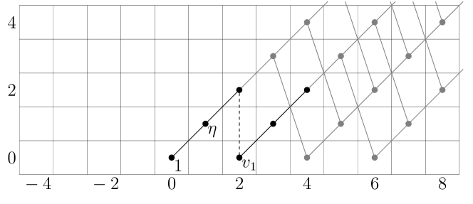
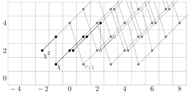
Figure 5. Patterns for the differentials on certain classes in the spectral sequences (8.3.2) and (8.3.3). The top figure illustrates the differential pattern on the unit $1$ and the bottom figure the differential pattern on $\chi$ and $\chi^{2}$. There, a $\circ$ denotes a copy of $\mathbb{F}_{2}$ generated by an $\eta$-multiple of the class $\eta v_{1}{{\chi}}+v_{1}^{2}{{\chi}}^{2}$. The dashed lines denote the extension by $2$ at $E_{\infty}$.

We now come to one the main calculations of this paper, 8.3.3. This result shows that the localized Adams-Novikov Spectral Sequence (8.3.3) for the spectrum $L_{K(1)}L_{K(2)}V(0)$ can be obtained from the spectral sequence of (8.3.2) for $L_{K(1)}(E^{h\mathbb{G}_{2}^{1}}\wedge V(0))$ by tensoring with the exterior algebra $E(\zeta_{2})$ and extending the differentials by the Leibniz rule. This is by no means formal. It requires a statement and argument which, on the surface, looks like a repetition of 8.3.2, but the logic requires us to prove part (2) of 8.3.2 before proving part (1) of 8.3.3.

Theorem 8.3.3.

The spectral sequence

(8.3.3) $$v_{1}^{-1}H_{c}^{*}(\mathbb{G}_{2},(E_{2})_{*}V(0))\Longrightarrow\pi_{*}L_{K(1)}L_{K(2)}V(0).$$

collapses at $E_{4}$. We have

1. The classes ${{\chi}}$, ${{\chi}}^{2}$, and $v_{1}{{\chi}}^{2}$, are permanent cycles. If $y$ is any class detected by ${{\chi}}$, then $\beta(y)$ is detected by ${{\chi}}^{2}$, and $2y=\beta(y)\eta$.

2. The spectral sequence collapses at $E_{4}$. The non-trivial differentials are determined by the differential

   $$d_{3}(v_{1}\chi)=\eta^{2}\chi^{2}$$

   and the fact that the spectral sequence is a module over $\mathbb{F}_{2}[v_{1}^{\pm 4},\eta]\otimes E(\sigma,\zeta_{2})$.

3. The class $\eta v_{1}{{\chi}}+v_{1}^{2}{{\chi}}^{2}$ is a permanent cycle. If $x$ is any class detected by $\eta v_{1}{{\chi}}+v_{1}^{2}{{\chi}}^{2}$, then $\beta(x)$ is detected by $\eta^{2}\chi+\eta v_{1}\chi^{2}$, and $2x=\beta(x)\eta$.

Proof.

We have

$$\mathbb{F}_{2}[v_{1}^{\pm 1},\eta]\otimes E(\sigma,\zeta_{2})\otimes\mathbb{F}_{2}[{{\chi}}]/({{\chi}}^{3})\cong v_{1}^{-1}H_{c}^{*}(\mathbb{G}_{2},(E_{2})_{*}V(0))\ .$$

We begin with part (1). The class ${{\chi}}$ is a $d_{3}$-cycle by 7.1.1. Thus, by parts (3) and (5) of 8.3.1, ${{\chi}}$ will be a permanent cycle if it is a $d_{5}$-cycle. Using part (4) of 8.3.1, we see that the only possible non-zero differential is

$$d_{5}({{\chi}})=v_{1}^{-4}\zeta_{2}\sigma\eta^{2}{{\chi}}^{2}.$$

However, by naturality with respect to the map $\mathbb{G}_{2}^{1}\to\mathbb{G}_{2}$ and by part (2) of 8.3.2, we have $d_{3}(v_{1}{{\chi}})=\eta^{2}{{\chi}}^{2}+\zeta_{2}x$ for some class $x\in E_{2}^{4,4}$. Since $\zeta_{2}^{2}=0$ in $H_{c}^{\ast}(\mathbb{G}_{2},E_{\ast})$, we can calculate

$$d_{3}(v_{1}^{-4}\zeta_{2}\sigma v_{1}{{\chi}})=v_{1}^{-4}\zeta_{2}\sigma d_{3}(v_{1}{{\chi}})=v_{1}^{-4}\zeta_{2}\sigma\eta^{2}{{\chi}}^{2}\ .$$

Hence $v_{1}^{-4}\zeta_{2}\sigma\eta^{2}{{\chi}}^{2}$ is zero on the $E_{4}$-term. We conclude that ${{\chi}}$ is a $d_{5}$-cycle. The remainder of the proof of part (1) goes through exactly as for part (1) of 8.3.2.

We now turn to part (2). As in part (2) of 8.3.2, there must be a class $a\in E_{3}^{1,2}$ with $d_{3}(a)=\eta^{2}{{\chi}}^{2}$. The vector space $E_{3}^{1,2}$ has basis $v_{1}{{\chi}}$, $v_{1}\zeta_{2}$, $v_{1}^{-3}\sigma$. The class $v_{1}\zeta_{2}$ is a permanent cycle by (1) and (3) of 8.3.1. The class $v_{1}^{-3}\sigma$ is a permanent cycle exactly as in the proof of (2) in 8.3.2 . Thus we have the indicated differential.

To get the collapse at $E_{4}$ we use 8.3.1 parts (1), (2), (3), and (5). Part (3) is proved exactly as in part (3) of 8.3.2. ∎

Remark 8.3.4.

We have not listed all the additive extensions in the spectral sequences (8.3.2) and (8.3.3). In fact we have missed only those exotic extensions by $2$ implied by the extension from $v_{1}$ to $\eta^{2}$ already visible in Figure 1 of Section 3. Indeed, it will follow from 8.4.4 below that all additive extensions are determined by $v_{1}^{4}$ and $\zeta_{2}$ multiplications and the exotic extensions by $2$ from $v_{1}$ to $\eta^{2}$, from ${{\chi}}$ to ${{\chi}}^{2}\eta$, and from $\eta v_{1}{{\chi}}+v_{1}^{2}{{\chi}}^{2}$ to

$$\eta^{3}{{\chi}}+\eta^{2}v_{1}{{\chi}}^{2}\equiv\eta^{2}v_{1}{{\chi}}^{2}.$$

The last equivalence follows from the fact that $\eta^{3}=0$ at $E_{4}$. These extension are all shown in Figure 5. The upper figure shows a pattern from $L_{K(1)}V(0)$, and the lower figure shows a pattern from $L_{K(1)}(V(0)\wedge V(0))$. Compare Figure 1 and Figure 2.

8.4. The homotopy type of $L_{K(1)}L_{K(2)}S^{0}$

We are now ready to prove the decomposition of the $K(1)$-localization of $L_{K(2)}S^{0}$. To begin we define a key map.

Definition 8.4.1.

Choose a class

$$y\in\pi_{-1}L_{K(1)}L_{K(2)}V(0)$$

detected by ${{\chi}}\in v_{1}^{-1}H_{c}^{1}(\mathbb{G}_{2},E_{\ast}V(0))$; this is possible by 8.3.3. If $D(-)$ denotes the Spanier-Whitehead duality functor, we let

$$x\colon\Sigma^{-2}V(0)=\Sigma^{-1}DV(0){{\longrightarrow\ }}L_{K(1)}L_{K(2)}S^{0}\$$

be the SW-adjoint of $y$; that is, the image of $y$ under the isomorphism

$$[S^{-1},L_{K(1)}L_{K(2)}V(0)]\cong[\Sigma^{-1}DV(0),L_{K(1)}L_{K(2)}S^{0}].$$

Remark 8.4.2.

The class $y$ is not unique. Any two choices of $y$ differ by an element of higher Adams-Novikov filtration. This implies that $x$ is not unique. However, the proof of 8.4.4 below comes down to an Adams-Novikov Spectral Sequence argument, and we will see that any choice of class $x$ will do. 9.2.1 below will allow us to refine our choice.

We prove the following preliminary result. In Section 3.1, we gave a short analysis of $\pi_{\ast}(V(0)\wedge V(0))$. In 3.1.6 and (3.1.7), we named classes $i_{0}$ and $i_{1}$ of degree $0$ and $1$ respectively with the property that $\beta(i_{1})=i_{0}$, where $\beta$ is the Bockstein in homotopy as in 3.1.1.

Lemma 8.4.3.

Let $x$ be as in 8.4.1. Then under the map

$$x\wedge V(0)\colon\Sigma^{-2}V(0)\wedge V(0){{\longrightarrow\ }}L_{K(1)}L_{K(2)}V(0)$$

the class $(x\wedge V(0))_{\ast}(i_{0})$ is detected by ${{\chi}}^{2}$ and $(x\wedge V(0))_{\ast}(i_{1})$ is detected by ${{\chi}}$ in the spectral sequence

$$v_{1}^{-1}H_{c}^{s}(\mathbb{G}_{2},(E_{2})_{t}V(0))\Longrightarrow\pi_{t-s}L_{K(1)}L_{K(2)}V(0).$$

Proof.

Since $x$ is the SW-adjoint of $y$ and $y$ is detected by ${{\chi}}$, 3.1.7 implies $(x\wedge V(0))_{\ast}(i_{1})=y$ is detected by ${{\chi}}$. The same result shows that $(x\wedge V(0))_{\ast}(i_{0})=\beta(y)$. Then the Geometric Boundary Theorem (see 2.3.7) implies that $(x\wedge V(0))_{\ast}(i_{0})$ is detected by the algebraic Bockstein of ${{\chi}}$, which is exactly $\chi^{2}$. ∎

We now have maps

$$\iota\colon S^{0} {{\longrightarrow\ }}L_{K(2)}S^{0}$$

$$\zeta_{2}\colon S^{-1} {{\longrightarrow\ }}L_{K(2)}S^{0}$$

$$x\colon\Sigma^{-2}V(0) {{\longrightarrow\ }}L_{K(1)}L_{K(2)}S^{0}$$

$$x\zeta_{2}\colon\Sigma^{-3}V(0) {{\longrightarrow\ }}L_{K(1)}L_{K(2)}S^{0}$$

The first of these maps is the unit; the second is the class of 2.2.1. These maps assemble into a map

(8.4.1) $$f=\iota\vee\zeta_{2}\vee x\vee x\zeta_{2}\colon S^{0}\vee S^{-1}\vee\Sigma^{-2}V(0)\vee\Sigma^{-3}V(0){{\longrightarrow\ }}L_{K(1)}L_{K(2)}S^{0}.$$

Here is one of our main results.

Theorem 8.4.4.

The map $f$ induces a $K(1)$-local equivalence

$$L_{K(1)}\big{(}S^{0}\vee S^{-1}\vee\Sigma^{-2}V(0)\vee\Sigma^{-3}V(0)\Big{)}\simeq L_{K(1)}L_{K(2)}S^{0}\ .$$

This is a consequence of 8.4.8, but to get there we need some preliminaries. The following result is standard.

Lemma 8.4.5.

Let $f\colon X_{1}\to X_{2}$ be a map of spectra. Suppose there is a type $n$ complex $Z$ so that $K(n)_{\ast}Z\neq 0$ and so that the induced map

$$L_{K(n)}(X_{1}\wedge Z)\to L_{K(n)}(X_{2}\wedge Z)$$

is an equivalence. Then $L_{K(n)}X_{1}\to L_{K(n)}X_{2}$ is an equivalence.

Proof.

It suffices to show that $K(n)_{*}f$ is an isomorphism. We have a diagram

The vertical maps are the Künneth isomorphisms for $K(n)_{*}$. Since $Z$ is of type $n$, $K(n)_{*}Z\neq 0$ and so is a faithful $K(n)_{*}$-module. Therefore, $K(n)_{*}f$ is an isomorphism. ∎

From this last result we see that it is enough to make a judicious choice of type $1$ complex. Recall that $Y=V(0)\wedge C(\eta)$. See Section 4.2.

Proposition 8.4.6.

There are isomorphisms of $\mathbb{F}_{2}[v_{1}^{\pm 1}]\otimes E(\sigma)$-modules

$$\mathbb{F}_{2}[v_{1}^{\pm 1}]\otimes E(\sigma)\otimes\mathbb{F}_{2}[{{\chi}}]/({{\chi}}^{3}) \cong v_{1}^{-1}H_{c}^{*}(\mathbb{G}_{2}^{1},E_{*}Y)$$

$$\mathbb{F}_{2}[v_{1}^{\pm 1}]\otimes E(\sigma,\zeta_{2})\otimes\mathbb{F}_{2}[{{\chi}}]/({{\chi}}^{3}) \cong v_{1}^{-1}H_{c}^{*}(\mathbb{G}_{2},E_{*}Y)\ .$$

Proof.

By Landweber exactness and 4.2.1 we have a short exact sequence of $\mathbb{G}_{2}$-modules

$$0\to E_{\ast}V(0)\to E_{\ast}Y\to E_{\ast}\Sigma^{2}V(0)\to 0\ .$$

Furthermore, in the long exact sequence in group cohomology, the boundary map is given be multiplication by $\eta$. We then get a long exact sequence for the localized cohomology groups $v_{1}^{-1}H_{c}^{*}(\mathbb{G}_{2},-)$ and the result follows from 8.2.5. ∎

Let $\iota\colon S^{0}\to Y$ be inclusion of the bottom cell and let $\zeta_{2}$ and $\sigma$ be the images of the same named class under the induced map

$$\iota_{*}\colon\pi_{*}L_{K(1)}L_{K(2)}S^{0}\to\pi_{*}L_{K(1)}L_{K(2)}Y\ .$$

Similarly, let $\jmath\colon V(0)\to Y$ be the inclusion of the bottom two cells; see(4.2.3). Let $y\in\pi_{-1}L_{K(1)}L_{K(2)}V(0)$ be as in 8.4.1 and call the images of $y$ and $\beta(y)$ under the induced map

$$\jmath_{*}\colon\pi_{*}L_{K(1)}L_{K(2)}V(0)\to\pi_{*}L_{K(1)}L_{K(2)}Y$$

by the same names.

Proposition 8.4.7.

The localized spectral sequence

$$v_{1}^{-1}H_{c}^{s}(\mathbb{G}_{2},(E_{2})_{t}Y)\Longrightarrow\pi_{t-s}L_{K(1)}L_{K(2)}Y$$

strongly converges, collapses at the $E_{2}$-term, and has no additive extensions.

Proof.

The $E_{2}$-term was calculated in 8.4.6. Convergence follows from 2.3.2 and 2.3.6. Since $Y$ has a $v_{1}$-self map, this is a spectral sequence of modules over $\mathbb{F}_{2}[v_{1}^{\pm 1}]\otimes E(\sigma,\zeta_{2})$. The class $\zeta_{2}$ is a permanent cycle by 2.2.1. The $E_{2}$-term has a horizontal vanishing line at $s=5$ and, by sparseness, $E_{2}=E_{3}$. By 7.1.1, the class ${{\chi}}$ is a $d_{3}$-cycle, and this forces the spectral sequence to collapse. It follows from 8.3.3 that $y$ is detected by ${{\chi}}$ and $\beta(y)$ is detected by ${{\chi}}^{2}$.

We turn to extensions; to do this, we must show $2$ annihilates the homotopy of $\pi_{\ast}L_{K(1)}L_{K(2)}Y$. In fact, we have

$$0=2\colon L_{K(1)}L_{K(2)}Y{{\longrightarrow\ }}L_{K(1)}L_{K(2)}Y.$$

To see this, recall that in 4.2.3 we showed there is a factoring

where $\nu\in\pi_{3}S^{0}$ is the Hopf map and $p$ is collapse onto the top cell. In 4.2.3, we also showed that $0=\nu\in\pi_{\ast}L_{K(1)}Y$; hence,

$$0=\nu\in\pi_{\ast}L_{K(1)}L_{K(2)}Y.\qed$$

8.4.4 now follows from 8.4.5 and the next result.

Theorem 8.4.8.

The map $f$ of (8.4.1) induces a $K(1)$-local equivalence

$$L_{K(1)}\big{(}S^{0}\vee S^{-1}\vee\Sigma^{-2}V(0)\vee\Sigma^{-3}V(0)\Big{)}\wedge Y\simeq L_{K(1)}L_{K(2)}Y\ .$$

Proof.

As a module over $\mathbb{F}_{2}[v_{1}^{\pm 1}]\otimes E(\sigma)$, $\pi_{\ast}L_{K(1)}Y$ is free of rank $1$ on a class $\iota$ of degree $0$ and $\pi_{\ast}L_{K(1)}(Y\wedge V(0))$ is free of rank $2$ on the classes $i_{0}$ and $i_{1}$ of degrees $0$ and $1$ respectively. See 4.2.2, 4.2.4, and the remarks before 4.2.4. By 8.4.6 and 8.4.7 we have that $\pi_{\ast}L_{K(1)}L_{K(2)}Y$ is free of rank $6$ over $\mathbb{F}_{2}[v_{1}^{\pm 1}]\otimes E(\sigma)$ on generators $\iota$, $\zeta_{2}$, $y$, $\beta(y)$, $\zeta_{2}y$ and $\zeta_{2}\beta(y)$ of degrees $0$, $-1$, $-1$, $-2$, $-2$ and $-3$ respectively. See the remarks before 8.4.7 as well.

We show that the maps

$$\iota\wedge Y\colon \ L_{K(1)}Y{{\longrightarrow\ }}L_{K(1)}L_{K(2)}Y$$

$$\zeta_{2}\wedge Y\colon \ \Sigma^{-1}L_{K(1)}Y{{\longrightarrow\ }}L_{K(1)}L_{K(2)}Y$$

$$x\wedge Y\colon \ \Sigma^{-2}L_{K(1)}(V(0)\wedge Y){{\longrightarrow\ }}L_{K(1)}L_{K(2)}Y$$

$$x\zeta_{2}\wedge Y\colon \ \Sigma^{-3}L_{K(1)}(V(0)\wedge Y){{\longrightarrow\ }}L_{K(1)}L_{K(2)}Y$$

are all injective on homotopy and exhaust the various summands.

The map

$$\iota\wedge Y\colon L_{K(1)}(S^{0}\wedge Y)\to L_{K(1)}L_{K(2)}(S^{0}\wedge Y)$$

is injective on homotopy and maps onto the $\mathbb{F}_{2}[v_{1}^{\pm 1}]\otimes E(\sigma)$ summand generated by $\iota$. Similarly $\zeta_{2}\wedge Y$ maps injectively onto the summand generated by $\zeta_{2}$.

This leaves the other four summands. Using the inclusion $\jmath\colon V(0)\to Y$ and 8.4.3 we have that

$$x\wedge Y\colon\Sigma^{-2}L_{K(1)}(V(0)\wedge Y){{\longrightarrow\ }}L_{K(1)}L_{K(2)}Y$$

sends the generators $i_{0}$ and $i_{1}$ in degrees $-2$ and $-1$ to non-zero classes detected by ${{\chi}}^{2}$ and ${{\chi}}$ respectively. By multiplying with $\zeta_{2}$ we can conclude that

$$x\zeta_{2}\wedge Y\colon\Sigma^{-3}L_{K(1)}(V(0)\wedge Y){{\longrightarrow\ }}L_{K(1)}L_{K(2)}Y$$

sends the generators $i_{0}$ and $i_{1}$ in degrees $-3$ and $-2$ to non-zero classes detected by ${{\chi}}^{2}\zeta_{2}$ and ${{\chi}}\zeta_{2}$ respectively. Since $y$ is detected by ${{\chi}}$ and $\beta(y)$ by ${{\chi}}^{2}$, the result follows from 8.4.6. ∎

8.5. The homotopy types of $L_{0}L_{K(2)}S^{0}$ and $L_{1}L_{K(2)}S^{0}$

We end this section by recording one of the main consequences of 8.4.4, which was stated in the introduction as 1.1.3. Recall that $X_{p}$ denote the $p$-completion of $X$.

Theorem 8.5.1 (Chromatic Splitting).

There is an equivalence

$$L_{1}L_{K(2)}S^{0}\simeq L_{1}(S^{0}_{2}\vee S^{-1}_{2})\vee L_{0}(S^{-3}_{2}\vee S^{-4}_{2})\vee L_{1}(\Sigma^{-2}V(0)\vee\Sigma^{-3}V(0))\ .$$

8.5.1 is proved exactly as in Theorem 5.11 of [GHM14], i.e. by examining the homotopy pull-back

For this, we need the following result which describes $L_{0}L_{K(2)}S^{0}$.

Theorem 8.5.2.

There is an equivalence

$$L_{0}L_{K(2)}S^{0}\simeq L_{0}(S^{0}_{2}\vee S^{-1}_{2}\vee S^{-3}_{2}\vee S^{-4}_{2}).$$

Proof.

By 6.2.2, the spectral sequence

$$E_{2}^{s,t}=H_{c}^{s}(\mathbb{G}_{2},E_{t})\otimes\mathbb{Q}\Longrightarrow\pi_{t-s}L_{0}L_{K(2)}S^{0}_{2}.$$

has $E_{2}$-term $E_{\mathbb{Q}_{2}}(\zeta_{2},e)$. It collapses with no extensions for degree reasons, and it converges by 2.3.2 and 2.3.6.

The homotopy classes detected by $1$, $\zeta_{2}$, $e$, $e\zeta_{2}$ combine to give a map

$$S^{0}_{2}\vee S^{-1}_{2}\vee S^{-3}_{2}\vee S^{-4}_{2}\to L_{0}L_{K(2)}S^{0}$$

which is a rational equivalence. ∎

9. Lifting to $L_{K(2)}S^{0}$

In Section 8 we constructed a map

$$x\vee x\zeta_{2}:\Sigma^{-2}V(0)\vee\Sigma^{-3}V(0){{\longrightarrow\ }}L_{K(1)}L_{K(2)}S^{0}$$

which became part of our $K(1)$-equivalence. The map $x$, which appeared in 8.4.1, was not unique, but any choice yielded the equivalence. In this section we show that there is a choice for this map that factors through the localization map

$$L_{K(2)}S^{0}\to L_{K(1)}L_{K(2)}S^{0}.$$

This is important for the chromatic assembly process.

The map $x$ is defined in 8.4.1 to be SW adoint to a class

$$y\in\pi_{-1}L_{K(1)}L_{K(2)}V(0)$$

detected by ${{\chi}}={{\chi}}_{2}\in v_{1}^{-1}H_{c}^{1}(\mathbb{G}_{2},E_{\ast}V(0))$. The key result of this section is 9.2.1, which shows that there is a choice of $y$ in the image of the map from $\pi_{-1}L_{K(2)}V(0)$.

There are two main steps: we first show $\pi_{-1}(E^{h\mathbb{G}_{2}^{1}}\wedge V(0))\cong{{\mathbb{Z}}}/4$ generated by a class detected by ${{\chi}}\in H_{c}^{1}(\mathbb{G}_{2}^{1},E_{0}/2)$; this uses the topological duality spectral sequence of 2.5.5. We then show this generator is in the image of the map

$$\pi_{-1}L_{K(2)}V(0){{\longrightarrow\ }}\pi_{-1}(E^{h\mathbb{G}_{2}^{1}}\wedge V(0))$$

using entirely different information, ultimately going back to 7.1.1.

9.1. Computing $\pi_{i}E^{h\mathbb{G}_{2}^{1}}$, $-3\leq i\leq 0$

For this calculation we use the topological duality spectral sequence of 2.5.6:

$$\pi_{q}\scr{E}_{p}\Longrightarrow\pi_{q-p}E^{h\mathbb{S}_{2}^{1}}.$$

We will use Lemmas 2.2.2 and 2.2.3 to deduce information about $\pi_{\ast}E^{h\mathbb{G}_{2}^{1}}$. The result is recorded in 9.1.5. The homotopy of $E^{h\mathbb{G}_{2}^{1}}$ in the indicated range is given in 9.1.6.

The first step is to record what we need about the homotopy groups of the fibers $\scr{E}_{p}$. Since we will be trying to compute $\pi_{i}E^{h\SS_{2}^{1}}$ for $i$ near $0$, we will only need information in a small range of dimensions.

Remark 9.1.1.

If $p=0$, then $\scr{E}_{p}=E^{hG_{24}}$; if $p=3$, then $\scr{E}_{p}=\Sigma^{48}E^{hG_{24}}$. Write $G_{48}=G_{24}\rtimes\mathop{\mathrm{Gal}}\nolimits$. Then the computation of $\pi_{\ast}E^{hG_{48}}$ can be mined from [Bau08] or [DFHH14]; it is very elaborate, but the part we need is fairly simple. We then have $\pi_{\ast}E^{hG_{24}}\cong{{\mathbb{W}}}\otimes\pi_{\ast}E^{hG_{48}}$. See 2.2.3.

Recall from 2.4.7 that there are classes $c_{4}$, $c_{6}$, $\Delta$, and $j$ in $H^{0}(G_{48},E_{\ast})$, of degrees $8$, $12$, $24$, and $0$ respectively, and an isomorphism

$${{\mathbb{Z}}}_{2}[[j]][c_{4},c_{6},\Delta^{\pm 1}]/I\cong H^{0}(G_{48},E_{\ast})$$

where $I$ is the ideal generated by

$$c_{4}^{3}-c_{6}^{2}=(12)^{3}\Delta\qquad\mathrm{and}\qquad j\Delta=c_{4}^{3}.$$

The class $j$ is a permanent cycle. The class $\Delta^{-2}$ is not a permanent cycle, but $4\Delta^{-2}$ and $j\Delta^{-2}$ are. This will explain the complicated form of $\pi_{-48}E^{hG_{24}}$ in (9.1.1) and the factor of $4$ in part (1) of 9.1.6. See also 6.2.3. Let $\eta$ and $\nu$ be the Hopf classes in the homotopy groups of spheres.

We pause to explain some notation. All homotopy groups $\pi_{\ast}E^{hG_{24}}$ are modules over ${{\mathbb{W}}}[[j]]\cong\pi_{0}E^{hG_{24}}$. For a quotient ring $R$ of ${{\mathbb{W}}}[[j]]$ we write $R\{x\}$ for the free $R$-module generated by $x$. If $J\subseteq R$ is an ideal, we write $J\{x\}\subseteq R\{x\}$ for the sub-$R$-module generated by $J$. The name of a generator, if given, is the label given to the class in the cohomology $H^{\ast}(G_{24},E_{\ast})\cong{{\mathbb{W}}}\otimes_{{{\mathbb{Z}}}_{2}}H^{\ast}(G_{48},E_{\ast})$ which detects the element in question. In all the degrees we list, $\pi_{i}E^{hG_{24}}$ is a sub-${{\mathbb{W}}}[[j]]$-module of a single cohomology group $E_{2}^{s,t}\cong H^{s}(G_{24},E_{t})$, and we indicate that cohomology group.

With this in mind we now record the homotopy groups we need.

(9.1.1) $$\pi_{i}E^{hG_{24}}\cong\begin{cases}\mathbb{W}[[j]]\cong E_{2}^{0,0}&i=0\\ \mathbb{F}_{4}[[j]]\{\eta^{i}\}\cong E_{2}^{i,2i}&i=1,2\\ {{\mathbb{W}}}/8\{\nu\}\cong E_{2}^{1,4}&i=3\\ 0&i=-3,-2,-1\\ (4,j)\{\Delta^{-2}\}\subseteq\mathbb{W}[[j]]\{\Delta^{-2}\}\cong E_{2}^{0,\text{-}48}&i=-{48}\\ (j)\{\eta\Delta^{-2}\}\subseteq\mathbb{F}_{4}[[j]]\{\eta\Delta^{-2}\}\cong E_{2}^{1,\text{-}46}&i=-47\\ (j)\{\eta^{2}\Delta^{-2}\}\subseteq\mathbb{F}_{4}[[j]]\{\eta^{2}\Delta^{-2}\}\cong E_{2}^{2,\text{-}44}&i=-46\\ \mathbb{W}/8\{\nu\Delta^{-2}\}\cong E_{2}^{1,\text{-}44}&i=-45\end{cases}$$

The edge homomorphism $h\mskip 0.5mu\colon\thinspace\pi_{i}E^{hG_{24}}\to E_{i}^{G_{24}}$ is an isomorphism when $i=0$ and injective when $i=-48$.

If $p=1$ or $2$, then $F_{p}=E^{hC_{6}}$. The following computation is relatively simple and can be read off of Section 4 of [MR09] or, more explicitly, from Section 2 of [BG18]. The notation is analogous to that in (9.1.1), except that $\pi_{3}E^{hC_{6}}\cong E_{\infty}^{3,6}$ is only a quotient of $E_{2}^{3,6}$.

(9.1.2) $$\pi_{i}E^{hC_{6}}\cong\begin{cases}0&i=-1,-2\\ \mathbb{W}[[u_{1}^{3}]]\cong E_{2}^{0,0}&i=0\\ \mathbb{F}_{4}[[u_{1}^{3}]]\{\eta^{i}\}\cong E_{2}^{i,2i}&i=1,2\\ \mathbb{F}_{4}\{\nu\}&i=3\\ \end{cases}$$

The edge homomorphism $h\mskip 0.5mu\colon\thinspace\pi_{0}E^{hC_{6}}\to E_{0}^{C_{6}}$ of the homotopy fixed point spectral sequence is an isomorphism.

Finally, we will need the following result in our calculations below.

Lemma 9.1.2.

Let $G=G_{24}$ and $G=C_{6}$. Multiplication by $\eta$ induces isomorphisms

$$\eta\colon H^{0}(G,E_{0}/2) \mathop{{{\longrightarrow\ }}}^{\cong}H^{1}(G,E_{2}/2)$$

$$\eta^{2}\colon H^{0}(G,E_{0}/2) \mathop{{{\longrightarrow\ }}}^{\cong}H^{2}(G,E_{4}/2).$$

Furthermore, for $i=1,2$ reduction modulo $2$ induces an isomorphism

Proof.

For these statements we will need some information about $H^{s}(G,E_{t})$ for low values of $s$ and $t$. There are many references for this; see [MR09] for $C_{6}$, [DFHH14] for $G_{24}$, or §2 of [BG18] for more references and a convenient chart for $G=G_{24}$.

From these references we see that there are isomorphisms

We also have that $H^{s}(G,E_{t})=0$ for $(s,t)=(1,0)$, $(2,2)$, and $(3,4)$. The result follows from the long exact sequence in group cohomology induced by the short exact sequence

$$\lx@xy@svg{\hbox{\raise 0.0pt\hbox{\kern 5.5pt\hbox{\ignorespaces\ignorespaces\ignorespaces\hbox{\vtop{\kern 0.0pt\offinterlineskip\halign{\entry@#!@&&\entry@@#!@\cr&&&&\crcr}}}\ignorespaces{\hbox{\kern-5.5pt\raise 0.0pt\hbox{\hbox{\kern 0.0pt\raise 0.0pt\hbox{\hbox{\kern 3.0pt\raise 0.0pt\hbox{$\textstyle{0\ignorespaces\ignorespaces\ignorespaces\ignorespaces}$}}}}}}}\ignorespaces\ignorespaces\ignorespaces\ignorespaces{}{\hbox{\lx@xy@droprule}}\ignorespaces{\hbox{\kern 29.5pt\raise 0.0pt\hbox{\hbox{\kern 0.0pt\raise 0.0pt\hbox{\lx@xy@tip{1}\lx@xy@tip{-1}}}}}}{\hbox{\lx@xy@droprule}}{\hbox{\lx@xy@droprule}}{\hbox{\kern 29.5pt\raise 0.0pt\hbox{\hbox{\kern 0.0pt\raise 0.0pt\hbox{\hbox{\kern 3.0pt\raise 0.0pt\hbox{$\textstyle{E_{\ast}\ignorespaces\ignorespaces\ignorespaces\ignorespaces}$}}}}}}}\ignorespaces\ignorespaces\ignorespaces\ignorespaces{}{\hbox{\lx@xy@droprule}}\ignorespaces\ignorespaces\ignorespaces{\hbox{\kern 50.78607pt\raise 5.54723pt\hbox{{}\hbox{\kern 0.0pt\raise 0.0pt\hbox{\hbox{\kern 3.0pt\hbox{\hbox{\kern 0.0pt\raise-1.9639pt\hbox{$\scriptstyle{\times 2}$}}}\kern 3.0pt}}}}}}\ignorespaces{\hbox{\kern 70.2583pt\raise 0.0pt\hbox{\hbox{\kern 0.0pt\raise 0.0pt\hbox{\lx@xy@tip{1}\lx@xy@tip{-1}}}}}}{\hbox{\lx@xy@droprule}}{\hbox{\lx@xy@droprule}}{\hbox{\kern 70.2583pt\raise 0.0pt\hbox{\hbox{\kern 0.0pt\raise 0.0pt\hbox{\hbox{\kern 3.0pt\raise 0.0pt\hbox{$\textstyle{E_{\ast}\ignorespaces\ignorespaces\ignorespaces\ignorespaces}$}}}}}}}\ignorespaces\ignorespaces\ignorespaces\ignorespaces{}{\hbox{\lx@xy@droprule}}\ignorespaces{\hbox{\kern 111.0166pt\raise 0.0pt\hbox{\hbox{\kern 0.0pt\raise 0.0pt\hbox{\lx@xy@tip{1}\lx@xy@tip{-1}}}}}}{\hbox{\lx@xy@droprule}}{\hbox{\lx@xy@droprule}}{\hbox{\kern 111.0166pt\raise 0.0pt\hbox{\hbox{\kern 0.0pt\raise 0.0pt\hbox{\hbox{\kern 3.0pt\raise 0.0pt\hbox{$\textstyle{E_{\ast}/2\ignorespaces\ignorespaces\ignorespaces\ignorespaces}$}}}}}}}\ignorespaces\ignorespaces\ignorespaces\ignorespaces{}{\hbox{\lx@xy@droprule}}\ignorespaces{\hbox{\kern 163.9971pt\raise 0.0pt\hbox{\hbox{\kern 0.0pt\raise 0.0pt\hbox{\lx@xy@tip{1}\lx@xy@tip{-1}}}}}}{\hbox{\lx@xy@droprule}}{\hbox{\lx@xy@droprule}}{\hbox{\kern 163.9971pt\raise 0.0pt\hbox{\hbox{\kern 0.0pt\raise 0.0pt\hbox{\hbox{\kern 3.0pt\raise 0.0pt\hbox{$\textstyle{0.}$}}}}}}}\ignorespaces}}}}\ignorespaces\qed \textstyle{0\ignorespaces\ignorespaces\ignorespaces\ignorespaces} \textstyle{E_{\ast}\ignorespaces\ignorespaces\ignorespaces\ignorespaces} \scriptstyle{\times 2} \textstyle{E_{\ast}\ignorespaces\ignorespaces\ignorespaces\ignorespaces} \textstyle{E_{\ast}/2\ignorespaces\ignorespaces\ignorespaces\ignorespaces} \textstyle{0.} \textstyle{0\ignorespaces\ignorespaces\ignorespaces\ignorespaces} \textstyle{E_{\ast}\ignorespaces\ignorespaces\ignorespaces\ignorespaces} \scriptstyle{\times 2} \textstyle{E_{\ast}\ignorespaces\ignorespaces\ignorespaces\ignorespaces} \textstyle{E_{\ast}/2\ignorespaces\ignorespaces\ignorespaces\ignorespaces} \textstyle{0.}$$

We now begin our calculation of the topological duality spectral sequence for $E^{h\SS_{2}^{1}}$. The result is illustrated in Figure 6. The main calculations needed to produce the $E_{2}$-term can be found in 6.1.3 and 9.1.5. There is an explanatory remark for these charts immediately following.

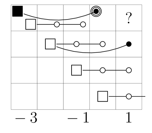
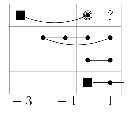
Figure 6. The $E_{1}$ (left) and $E_{2}$ (right) terms of the TDSS for $\pi_{*}(E^{h\mathbb{S}_{2}^{1}})$.

Remark 9.1.3.

The two charts are respectively the $E_{1}$-term and $E_{2}$-term of the topological duality spectral sequence of 2.5.6 for $\pi_{*}(E^{h\mathbb{S}_{2}^{1}})$. We use the Adams grading with $E_{1}^{p,q}$ in 2.5.6 in the $(q-p,p)$ box.

A $\Box$ denotes a copy of $\mathbb{W}[[j]]$ if $s=0,3$ and $\mathbb{W}[[u_{1}^{3}]]$ if $s=1,2$. Similarly, a $\circ$ denotes a copy of $\mathbb{F}_{4}[[j]]$ or $\mathbb{F}_{4}[[u_{1}^{3}]]$. A $\bullet$ is a copy of $\mathbb{F}_{4}$. A $\blacksquare$ is a copy of $\mathbb{W}$. The symbol denotes a copy of $\mathbb{W}/8$.

Horizontal and curved lines indicate multiplication by $\eta$ respectively $\nu$. The dashed vertical line on the $E_{2}$-term is there to indicate the additive extension on the $E_{\infty}$-term. See 9.1.5. In the top row of the left chart, we have depicted the ideal $(4,j)\{\Delta^{-2}\}\subseteq\pi_{-48}E^{hG_{24}}$ using the ${{\mathbb{W}}}$-module structure as ${{\mathbb{W}}}\{4\}\oplus{{\mathbb{W}}}[[j]]\{j\}\subseteq{{\mathbb{W}}}[[j]]$. The $\blacksquare$ represents ${{\mathbb{W}}}\{4\}$ and the $\Box$ represents ${{\mathbb{W}}}[[j]]\{j\}$.

The upper right corners of both charts contribute to $\pi_{1}E^{h\SS_{2}^{1}}$. The elements in these spots do not support differentials in the topological duality spectral sequence, so don’t come into the calculations of $\pi_{0}$. As they don’t affect our answers, we don’t include them in the discussion and leave these boxes marked with a question mark.

We now come to the calculation of $\pi_{\ast}E^{h\SS_{2}^{1}}$ in the range we need. We compute using the topological duality spectral sequence of 2.5.6:

$$\lx@xy@svg{\hbox{\raise 0.0pt\hbox{\kern 23.24538pt\hbox{\ignorespaces\ignorespaces\ignorespaces\hbox{\vtop{\kern 0.0pt\offinterlineskip\halign{\entry@#!@&&\entry@@#!@\cr&\crcr}}}\ignorespaces{\hbox{\kern-23.24538pt\raise 0.0pt\hbox{\hbox{\kern 0.0pt\raise 0.0pt\hbox{\hbox{\kern 3.0pt\raise 0.0pt\hbox{$\textstyle{E_{1}^{p,q}=\pi_{q}\scr{E}_{p}\ignorespaces\ignorespaces\ignorespaces\ignorespaces}$}}}}}}}\ignorespaces\ignorespaces\ignorespaces\ignorespaces{}{\hbox{\hbox{\kern 0.0pt\raise 1.0pt\hbox{\lx@xy@droprule}}\hbox{\kern 0.0pt\raise-1.0pt\hbox{\lx@xy@droprule}}}}\ignorespaces{\hbox{\kern 47.24538pt\raise 0.0pt\hbox{\hbox{\kern 0.0pt\raise 0.0pt\hbox{\lx@xy@tip{1.5}\lx@xy@tip{-1.5}}}}}}{\hbox{\hbox{\kern 0.0pt\raise 1.0pt\hbox{\lx@xy@droprule}}\hbox{\kern 0.0pt\raise-1.0pt\hbox{\lx@xy@droprule}}}}{\hbox{\hbox{\kern 0.0pt\raise 1.0pt\hbox{\lx@xy@droprule}}\hbox{\kern 0.0pt\raise-1.0pt\hbox{\lx@xy@droprule}}}}{\hbox{\kern 47.24538pt\raise 0.0pt\hbox{\hbox{\kern 0.0pt\raise 0.0pt\hbox{\hbox{\kern 3.0pt\raise 0.0pt\hbox{$\textstyle{\pi_{q-p}(E_{2}^{h\mathbb{S}_{2}^{1}})}$}}}}}}}\ignorespaces}}}}\ignorespaces. \textstyle{E_{1}^{p,q}=\pi_{q}\scr{E}_{p}\ignorespaces\ignorespaces\ignorespaces\ignorespaces} \textstyle{\pi_{q-p}(E_{2}^{h\mathbb{S}_{2}^{1}})} \textstyle{E_{1}^{p,q}=\pi_{q}\scr{E}_{p}\ignorespaces\ignorespaces\ignorespaces\ignorespaces} \textstyle{\pi_{q-p}(E_{2}^{h\mathbb{S}_{2}^{1}})}$$

We will use information from 9.1.1. The $E_{1}$-term is displayed in Figure 6. The notation $\Delta_{0}$, $b_{0}$, $\overline{b}_{0}$, and $\overline{\Delta}_{0}$ was explained in 5.2.5.

Theorem 9.1.4.

There are isomorphisms

1. $\pi_{-3}(E^{h\mathbb{S}_{2}^{1}})\cong{{\mathbb{W}}}$ with generator detected by $4\overline{\Delta}_{0}\in E_{1}^{3,0}=\pi_{0}\Sigma^{48}E^{hG_{24}}$.

2. $\pi_{-2}(E^{h\mathbb{S}_{2}^{1}})\cong\mathbb{F}_{4}$ detected by $\overline{b}_{0}\in E_{1}^{2,0}=\pi_{0}E^{hC_{6}}$.

3. $\pi_{-1}(E^{h\mathbb{S}_{2}^{1}})\cong\mathbb{F}_{4}$ with generator detected by $\eta\overline{b}_{0}$ in $E_{1}^{2,1}=\pi_{1}E^{hC_{6}}$.

4. $\pi_{0}(E^{h\mathbb{S}_{2}^{1}})\cong\mathbb{W}\oplus\mathbb{W}/4\oplus\mathbb{W}/8$.

Furthermore, for $\pi_{0}E^{h\SS_{2}^{1}}$,

1. a generator of the summand ${{\mathbb{W}}}$ is detected by the unit in $E_{1}^{0,0}=\pi_{0}E^{hG_{24}}$;

2. a generator of the summand $\mathbb{W}/4$ is detected by $\eta b_{0}\in E_{1}^{1,1}=\pi_{1}E^{hC_{6}}$;

3. a generator of the summand ${{\mathbb{W}}}/8$ is detected by $\nu\overline{\Delta}_{0}\in E_{1}^{3,3}=\pi_{3}\Sigma^{48}E^{hG_{24}}$.

If a class in $\pi_{0}E^{h\SS_{2}^{1}}$ is detected by $\eta b_{0}\in E_{1}^{1,1}$ then twice that class is detected by $\eta^{2}\overline{b}_{0}\in E_{1}^{2,2}\cong\pi_{2}E^{hC_{6}}$.

Proof.

This requires a multi-part argument and we break it into steps.

Calculating $d_{1}$ with $q=0$. The fundamental calculation is with the sequence

Using the calculations of 9.1.1, this can be fit into a diagram of chain complexes

The vertical maps down from the top row are edge homomorphisms. All but the last of these maps are isomorphisms. The last map is injective with image the ideal $(4,j)\subseteq{{\mathbb{W}}}[[j]]$. The map from the bottom to the middle row is induced by the unit map $i\colon{{\mathbb{W}}}\to E_{0}$; thus, by 6.1.3, the bottom two rows have the same cohomology. It then follows that in the topological duality spectral sequence we have

$$E_{2}^{0,0}\cong{{\mathbb{W}}}\qquad E_{2}^{1,0}=0\qquad E_{2}^{2,0}\cong\mathbb{F}_{4}\qquad E_{2}^{3,0}\cong{{\mathbb{W}}}.$$

The generator for $E_{2}^{2,0}$ is $\overline{b}_{0}$ and the generator for $E_{2}^{3,0}$ is $4\overline{\Delta}_{0}$.

Calculating $d_{1}$ with $q=1$. The next calculation is with the sequence

This can be fit into a diagram

Using the calculations of 9.1.1, we have all vertical maps from the top row are isomorphisms except the edge homomorphism on the right hand side. This is an inclusion onto the submodule $\mathbb{F}_{4}[[j]]\{j\eta\}\subseteq\mathbb{F}_{4}[[j]]\{\eta\}$. The maps from the second row to the third row are reduction modulo $2$ and the maps from the bottom row to the third row are multiplication by $\eta$. All are isomorphisms by 9.1.2. It follows that in the topological duality spectral sequence we have

$$E_{2}^{0,1}\cong\mathbb{F}_{4}\qquad E_{2}^{1,1}=\mathbb{F}_{4}\qquad E_{2}^{2,1}\cong\mathbb{F}_{4}\qquad E_{2}^{3,1}\cong 0.$$

The generator for $E_{2}^{0,1}$ is $\eta\Delta_{0}$, that for $E_{2}^{1,1}$ is $\eta b_{0}$ and the generator for $E_{2}^{2,1}$ is $\eta\overline{b}_{0}$.

Calculating $d_{1}$ with $q=2$. The exact same argument, with $\eta$ replaced by $\eta^{2}$, shows that

$$E_{2}^{0,2}\cong\mathbb{F}_{4}\qquad E_{2}^{1,2}=\mathbb{F}_{4}\qquad E_{2}^{2,2}\cong\mathbb{F}_{4}\qquad E_{2}^{3,2}\cong 0$$

and that the generator for $E_{2}^{0,2}$ is $\eta^{2}\Delta_{0}$, that for $E_{2}^{1,2}$ is $\eta^{2}b_{0}$ and the generator for $E_{2}^{2,2}$ is $\eta^{2}\overline{b}_{0}$.

Calculating $d_{1}$ with $q=3$. Finally, we calculate with the sequence

In this case we need a different style of argument. By 9.1.1 we have

$$E_{1}^{0,3}\cong{{\mathbb{W}}}/8\qquad E_{1}^{1,3}=\mathbb{F}_{4}\qquad E_{1}^{2,3}\cong\mathbb{F}_{4}\qquad E_{1}^{3,3}\cong{{\mathbb{W}}}/8$$

generated by $\nu\Delta_{0}$, $\nu b_{0}$, $\nu\overline{b}_{0}$, and $\nu\overline{\Delta}_{0}$ respectively. Then $d_{1}=0$ by the calculation for $q=0$ and the $\nu$-linearity of $d_{1}$.

Calculating $d_{2}$ and $d_{3}$. We first turn to $d_{2}$. By looking at Figure 6, we see that in the range $0\leq q-p\leq 1$, the only classes which could support a non-zero $d_{2}$ are the unit, detected by $\Delta_{0}$ and the classes detected by $\eta\Delta_{0}$ and $\eta^{2}b_{0}$ in $E_{2}^{0,1}$ and $E_{2}^{1,2}$. The unit and $\eta\Delta_{0}$ are evidently permanent cycles and $\eta^{2}b_{0}$ is an $\eta$-multiple of $\eta b_{0}$, which is permanent cycle. Thus $d_{2}=0$.

This leaves only $d_{3}$. But in the range $0\leq q-p\leq 1$, the only class which could support a non-zero $d_{3}$ is $\eta$ times the unit, so $d_{3}=0$ as well and we have shown

$$E_{2}^{p,q}\cong E_{\infty}^{p,q},\qquad-3\leq q-p\leq 0.$$

Settling extensions. At this point we have a filtration of the ${{\mathbb{W}}}$-module $\pi_{0}E^{hG_{24}}$

The unit $S^{0}\to E^{h\SS_{2}^{1}}$ induces a map ${{\mathbb{Z}}}_{2}\to\pi_{0}E^{h\SS_{2}^{1}}$ which extends to a Galois equivariant homomorphism $\mathbb{W}\to\pi_{0}E^{h\SS_{2}^{1}}$. This splits off the torsion-free summand. Thus we need only show that a generator of $E_{\infty}^{1,1}$ detects an element of order $4$. This follows from 3.1.5 and, in particular, from (3.1.4). Specifically, $\overline{b}_{0}\in E_{\infty}^{2,0}$ detects a unique Galois invariant homotopy class $z$ of order $2$ in $\pi_{-2}E^{h\SS_{2}^{1}}$. Since a generator $E_{\infty}^{2,2}$ is detected by $\eta^{2}\overline{b}_{0}$, we have $2\langle z,2,\eta\rangle=\eta^{2}z\neq 0$ and, in particular that $\langle z,2,\eta\rangle$ does not contain zero. Since $\langle z,2,\eta\rangle$ is Galois invariant, it can only be detected by $\eta b_{0}$. ∎

The next result describes how the generators of $\pi_{\ast}E^{h\SS_{2}^{1}}$ in our range are detected in the homotopy fixed point spectral sequence. In reading the statement, a bit of care is needed. The class $e$ is not a permanent cycle, so the class $\nu e$ of part (iii) is not a product; it is named by the class that detects it in the spectral sequence.

Theorem 9.1.5.

In the homotopy fixed point spectral sequence

$$H_{c}^{s}(\SS_{2}^{1},E_{t})\Longrightarrow\pi_{t-s}E^{h\SS_{2}^{1}}$$

1. a generator of $\pi_{-3}(E^{h\mathbb{S}_{2}^{1}})\cong{{\mathbb{W}}}$ is detected by $4e$ in $H_{c}^{3}(\SS_{2}^{1},E_{0})$;

2. a generator of $\pi_{-2}(E^{h\mathbb{S}_{2}^{1}})\cong\mathbb{F}_{4}$ is detected by ${\widetilde{\chi}}$ in $H_{c}^{2}(\SS_{2}^{1},E_{0})$;

3. a generator of $\pi_{-1}(E^{h\mathbb{S}_{2}^{1}})\cong\mathbb{F}_{4}$ is detected by $\eta{\widetilde{\chi}}$ in $H_{c}^{3}(\SS_{2}^{1},E_{2})$;

4. $\pi_{0}(E^{h\mathbb{S}_{2}^{1}})\cong\mathbb{W}\oplus\mathbb{W}/4\oplus\mathbb{W}/8$.

Furthermore, for $\pi_{0}E^{h\SS_{2}^{1}}$,

1. a generator of the summand ${{\mathbb{W}}}$ is detected by the unit in $H_{c}^{0}(\SS_{2}^{1},E_{0})$;

2. a generator of the summand $\mathbb{W}/4$ is detected by an element in the Massey product

   $${\langle{\widetilde{\chi}},2,\eta\rangle}\in H_{c}^{2}(\SS_{2}^{1},E_{1});$$

3. a generator of the summand ${{\mathbb{W}}}/8$ is detected by $\nu e\in H_{c}^{4}(\SS_{2}^{1},E_{4})$.

If a class in $\pi_{0}E^{h\SS_{2}^{1}}$ is detected by ${\langle{\widetilde{\chi}},2,\eta\rangle}$ then twice that class is detected by

$$\eta^{2}{\widetilde{\chi}}\in H_{c}^{4}(\SS_{2}^{1},E_{4}).$$

Proof.

This follows from 9.1.4 and 5.2.6, with judicious uses of 2.5.8.

For part (1) we know from 5.2.6 that $4\overline{\Delta}_{0}$ detects $4e$ in the algebraic duality spectral sequence, so 2.5.8 applies directly.

For part (2), the same result shows that $\overline{b}_{0}$ detects ${\widetilde{\chi}}$, and again we can use 2.5.8. Part (3) then follows from Part (2).

It remains to discuss $\pi_{0}E^{h\SS_{2}^{1}}$.

At the very end of the proof of 9.1.4 we argued that if $z\in\pi_{-2}E^{h\SS_{2}^{1}}$ and is the unique non-zero Galois invariant class, then the Toda bracket $\langle z,2,\eta\rangle$ does not contain zero and is detected in the topological duality spectral sequence by $\eta b_{0}$. This forces the Massey product ${\langle{\widetilde{\chi}},2,\eta\rangle}$ to be non-zero. Since $z$ is detected by ${\widetilde{\chi}}$ and $\eta^{2}z\neq 0$, the exotic extension follows from the standard juggling formula $2\langle z,2,\eta\rangle=\eta^{2}z$ of (3.1.4). ∎

We next pass to $\mathbb{G}^{1}_{2}$. The result is a corollary of 9.1.5 obtained by taking Galois fixed points.

Corollary 9.1.6.

There are isomorphisms

1. $\pi_{-3}E^{h\mathbb{G}_{2}^{1}}\cong{{\mathbb{Z}}}_{2}$ generated by a class detected by $4e\in H_{c}^{3}(\mathbb{G}_{2}^{1},E_{0})$;

2. $\pi_{-2}E^{h\mathbb{G}_{2}^{1}}\cong{{\mathbb{Z}}}/2$ generated by a class detected by ${\widetilde{\chi}}\in H_{c}^{2}(\mathbb{G}_{2}^{1},E_{0})$;

3. $\pi_{-1}E^{h\mathbb{G}_{2}^{1}}\cong{{\mathbb{Z}}}/2$ generated by a class detected by $\eta{\widetilde{\chi}}\in H_{c}^{3}(\mathbb{G}_{2}^{1},E_{2})$;

4. $\pi_{0}E^{h\mathbb{G}_{2}^{1}}\cong{{\mathbb{Z}}}_{2}\oplus{{\mathbb{Z}}}/4\oplus{{\mathbb{Z}}}/8$.

Furthermore, the summands of $\pi_{0}E^{h\mathbb{G}_{2}^{1}}$ are generated by the unit and classes detected by ${\langle{\widetilde{\chi}},2,\eta\rangle}\in H_{c}^{2}(\mathbb{G}_{2}^{1},E_{2})$ and $\nu e\in H_{c}^{4}(\mathbb{G}_{2}^{1},E_{4})$. If a class is detected by ${\langle{\widetilde{\chi}},2,\eta\rangle}$, then twice that class is detected by $\eta^{2}{\widetilde{\chi}}$.

For future reference we will also describe the multiplicative structure of $\pi_{0}E_{2}^{h\mathbb{G}_{2}^{1}}$.

Corollary 9.1.7.

In the kernel of the edge homomorphism of the Adams-Novikov Spectral Sequence

$$\pi_{0}E^{h\mathbb{G}_{2}^{1}}\to H^{0}(\mathbb{G}_{2}^{1},E_{0})$$

we have the following multiplicative relations.

1. The product of any two classes detected by $\nu e$ is $0$.

2. The product of any class detected by $\langle\widetilde{\chi},2,\eta\rangle$ and any class detected in filtration $4$ is trivial.

3. The product of two classes detected by $\langle\widetilde{\chi},2,\eta\rangle$ is detected by $\eta^{2}\widetilde{\chi}$ modulo $2\nu e$.

Proof.

Parts (1) and (2) are clear because in the spectral sequence

$$H^{s}_{c}(\mathbb{G}_{2}^{1},E_{t})\Longrightarrow\pi_{t-s}E^{h\mathbb{G}_{2}^{1}}$$

we have $E_{\infty}^{s,s}=0$ for $s>4$. This follows from 9.1.6.

For Part (3) we examine the reduction map map

$$H^{s}_{c}(\mathbb{G}_{2}^{1},E_{t}){{\longrightarrow\ }}H^{s}_{c}(\mathbb{G}_{2}^{1},E_{t}/2)$$

This map kills $2\nu e$. By definition is sends $\widetilde{\chi}$ to $\chi^{2}$; hence it sends the Massey product to $\eta\chi$. The result follows. ∎

Remark 9.1.8.

Using the fiber sequence of (2.2.4)

we can make analogous calculations for the sphere itself. For example

$$\pi_{-3}L_{K(2)}S^{0}\cong{{\mathbb{Z}}}_{2}\oplus{{\mathbb{Z}}}/2\subseteq H_{c}^{3}(\mathbb{G}_{2},E_{0})$$

generated by the classes $4e$ and $\zeta_{2}{\widetilde{\chi}}$.

We now pass to an analysis of $\pi_{\ast}(E^{h\mathbb{G}_{2}^{1}}\wedge V(0))$. Recall from Section 3.1 that $q$ and $j$ are defined by the cofiber sequence

From 3.1.1 we have $\beta=jq$. Let $z\colon S^{-2}\to E^{h\mathbb{G}_{2}^{1}}$ be the class detected by ${\widetilde{\chi}}$. Since this class has order two, it factors through

$$q\colon\Sigma^{-1}E^{h\mathbb{G}_{2}^{1}}\wedge V(0){{\longrightarrow\ }}E^{h\mathbb{G}_{2}^{1}}$$

and we get a map

(9.1.3) $$y_{1}\colon S^{-1}{{\longrightarrow\ }}E^{h\mathbb{G}_{2}^{1}}\wedge V(0).$$

such that $q_{*}(y_{1})=z$. We now have the following result.

Proposition 9.1.9.

There are isomorphisms

1. $\pi_{-1}(E^{h\mathbb{G}_{2}^{1}}\wedge V(0))\cong{{\mathbb{Z}}}/4$ generated by the class $y_{1}$. This class is detected by ${{\chi}}\in H_{c}^{1}(\mathbb{G}_{2}^{1},E_{0}/2)$.

2. $\pi_{-2}(E^{h\mathbb{G}_{2}^{1}}\wedge V(0))\cong{{\mathbb{Z}}}/2$. The generator is detected by ${{\chi}}^{2}\in H_{c}^{2}(\mathbb{G}_{2}^{1},E_{0}/2)$.

Furthermore, the class $2y_{1}$ is detected by $\eta{{\chi}}^{2}\in H_{c}^{3}(\mathbb{G}_{2}^{1},E_{2}/2)$.

Proof.

From 9.1.6 it follows that

$$\pi_{-2}(E^{h\mathbb{G}_{2}^{1}}\wedge V(0))\cong{{\mathbb{Z}}}/2$$

generated by $j_{*}(z)$. This class is detected by the image of ${\widetilde{\chi}}$ in $H_{c}^{2}(\mathbb{G}_{2}^{1},E_{0}/2)$, which is exactly ${{\chi}}^{2}$. From the same result we have a short exact sequence

$$0\to{{\mathbb{Z}}}/2\to\pi_{-1}(E^{h\mathbb{G}_{2}^{1}}\wedge V(0))\to{{\mathbb{Z}}}/2\to 0.$$

Since $j_{*}(z)$ is detected by the Bockstein on ${{\chi}}$ and $j_{*}(y_{1})=j_{*}q_{*}(z)=\beta(z)$, the Geometric Boundary Theorem (see 2.3.7) implies that the class $y_{1}$ is detected by ${{\chi}}$. The generator of the kernel is $\eta j_{*}(z)$, detected by $\eta\chi^{2}$. It remains to show $y_{1}$ has order $4$; this follows from 3.1.4. ∎

9.2. Producing the lifting

We now show that the class $y_{1}\in\pi_{-1}(E^{h\mathbb{G}_{2}^{1}}\wedge V(0))$ of order $4$ constructed above in 9.1.9 is in the image of the unit map $\pi_{\ast}L_{K(2)}V(0)\to\pi_{\ast}(E^{h\mathbb{G}_{2}^{1}}\wedge V(0))$. Recall from 8.3.3 that the class ${{\chi}}\in v_{1}^{-1}H_{c}^{1}(\mathbb{G}_{2},E_{\ast}V(0))$ is a non-zero permanent cycle in the localized Adams-Novikov Spectral Sequence computing $\pi_{\ast}L_{K(1)}L_{K(2)}V(0)$.

Theorem 9.2.1.

There is a class $y_{0}\in\pi_{-1}L_{K(2)}V(0)$ detected by ${{\chi}}\in H_{c}^{1}(\mathbb{G}_{2},E_{0}/2)$. Under the map

$$\pi_{-1}L_{K(2)}V(0){{\longrightarrow\ }}\pi_{-1}(E^{h\mathbb{G}_{2}^{1}}\wedge V(0))$$

the class $y_{0}$ maps to $y_{1}$ and under the map

$$\pi_{-1}L_{K(2)}V(0){{\longrightarrow\ }}\pi_{-1}L_{K(1)}L_{K(2)}V(0)$$

the class $y_{0}$ is non-zero and detected by the class ${{\chi}}\in v_{1}^{-1}H_{c}^{\ast}(\mathbb{G}_{2},E_{\ast}V(0))$.

Proof.

There is a fiber sequence

(9.2.1)

where $\pi\in\mathbb{G}_{2}$ is an element that generates $\mathbb{G}_{2}/\mathbb{G}_{2}^{1}\cong{{\mathbb{Z}}}_{2}$. Since $\pi_{-1}(E^{h\mathbb{G}_{2}^{1}}\wedge V(0))$ is isomorphic to ${{\mathbb{Z}}}/4$, we have that $\pi_{\ast}y_{1}=\pm y_{1}$ so either $(\pi-1)_{\ast}y_{1}=0$ or $(\pi-1)_{\ast}y_{1}=2y_{1}$.

If the first case applies, then we can choose a class $y_{2}\in\pi_{-1}L_{K(2)}V(0)$ which maps to $y_{1}$. By 6.1.7 we have an isomorphism

$$H_{c}^{1}(\mathbb{G}_{2},E_{0}V(0))\cong{{\mathbb{Z}}}/2\times{{\mathbb{Z}}}/2$$

with generators ${{\chi}}$ and $\zeta_{2}$. The class $\zeta_{2}$ maps to zero in $H_{c}^{1}(\mathbb{G}_{2}^{1},E_{0}V(0))$; hence, we have that $y_{2}$ is detected by ${{\chi}}+\epsilon\zeta_{2}$ where $\epsilon=0$ or $1$. Since $\zeta_{2}$ is a permanent cycle by 2.2.1 detecting a homotopy class also called $\zeta_{2}$, we set $y_{0}=y_{2}+\epsilon\zeta_{2}$. Then $y_{0}$ is detected by ${{\chi}}$. Finally, by 8.2.5, the map

$$H_{c}^{1}(\mathbb{G}_{2},E_{0}V(0))\to v_{1}^{-1}H_{c}^{\ast}(\mathbb{G}_{2},E_{\ast}V(0))$$

is an injection in degree $1$, so the final statement follows.

If the second case applies we would have that $y_{1}$ maps to a class of order $2$ in $\pi_{-2}L_{K(2)}V(0)$ under the boundary map in the long exact sequence in homotopy obtained from the cofiber sequence of (9.2.1). To rule this out, we use the following result, 9.2.2. ∎

Theorem 9.2.2.

Under the boundary homomorphism

$$\partial\colon\pi_{-1}(E^{h\mathbb{G}_{2}^{1}}\wedge V(0)){{\longrightarrow\ }}\pi_{-2}L_{K(2)}V(0)$$

the class $x_{1}=\partial(y_{1})$ is a class of exact order $4$ detected by ${{\zeta}}{{\chi}}\in H_{c}^{2}(\mathbb{G}_{2},E_{0}/2)$. The class $2x_{1}$ is detected by $\eta{{\zeta}}{{\chi}}^{2}\in H_{c}^{4}(\mathbb{G}_{2},E_{2}/2)$.

This is an application of the Geometric Boundary Theorem; see 2.3.7. The proof will be below, after we have given some background.

Since $E_{\ast}E^{\mathbb{G}_{2}^{1}}\cong\operatorname{map}_{cts}(\mathbb{G}_{2}/\mathbb{G}_{2}^{1},E_{\ast})$ we can apply $E_{\ast}$ to the cofiber sequence (9.2.1) and obtain a short exact sequence of Morava modules

(9.2.2)

and hence a diagram of spectral sequences

(9.2.3)

where $\delta$ is the algebraic connecting map

in the long exact sequence induced by the short exact sequence (9.2.2).

Lemma 9.2.3.

Suppose the class $a\in H_{c}^{s}(\mathbb{G}_{2}^{1},E_{*}/2)$ is the image of an element $b\in H_{c}^{s}(\mathbb{G}_{2},E_{*}/2)$ under the restriction

$$H_{c}^{s}(\mathbb{G}_{2},E_{*}/2)\to H_{c}^{s}(\mathbb{G}^{1}_{2},E_{*}/2)\ .$$

Then $\delta(a)={{\zeta}}_{2}b$.

Proof.

The connecting homomorphism $\delta$ is a homomorphism of $H_{c}^{*}(\mathbb{G}_{2},E_{*}/2)$-modules. By the definition of $\zeta_{2}$ (see 5.1.1), we have $\delta(1)=\zeta_{2}$, and the result follows. ∎

Proof of 9.2.2..

Using 9.2.3 and the diagram of spectral sequences (9.2.3) we have that $\partial(y_{1})\in\pi_{-2}L_{K(2)}V(0)$ is detected by ${{\zeta}}_{2}{{\chi}}\in H_{c}^{2}(\mathbb{G}_{2},E_{0}/2)$. Since $2y_{1}$ is detected by $\eta{{\chi}}^{2}$, we can again use 9.2.3 and the diagram of spectral sequences (9.2.3) to conclude that $\partial(2y_{1})\in\pi_{-2}L_{K(2)}V(0)$ is detected by

$${{\zeta}}_{2}\eta{{\chi}}^{2}\in H_{c}^{4}(\mathbb{G}_{2},E_{2}/2).$$

This class is non-zero by 8.2.5. Thus we need to check that this class cannot be a boundary in the spectral sequence. Since $E_{\ast}/2=0$ in odd degrees, the only possible differential is

$$d_{3}\colon H_{c}^{1}(\mathbb{G}_{2},E_{0}/2)\to H_{c}^{4}(\mathbb{G}_{2},E_{2}/2).$$

By 6.1.7 we have an isomorphism $H_{c}^{1}(\mathbb{G}_{2},E_{0}/2)\cong{{\mathbb{Z}}}/2\times{{\mathbb{Z}}}/2$ with generators ${{\zeta}}_{2}$ and ${{\chi}}$. We know by 2.2.1 that ${{\zeta}}_{2}$ is a permanent cycle and we know by 7.1.1 that ${{\chi}}$ is a $d_{3}$-cycle. Thus $d_{3}=0$ on $H_{c}^{1}(\mathbb{G}_{2},E_{0}/2)$ and the result follows. ∎

References

• [AM04] Alejandro Adem and R. James Milgram. Cohomology of finite groups, volume 309 of Grundlehren der Mathematischen Wissenschaften [Fundamental Principles of Mathematical Sciences]. Springer-Verlag, Berlin, second edition, 2004. URL: https://doi.org/10.1007/978-3-662-06280-7, doi:10.1007/978-3-662-06280-7.
• [Bau08] Tilman Bauer. Computation of the homotopy of the spectrum tmf. In Groups, homotopy and configuration spaces, volume 13 of Geom. Topol. Monogr., pages 11–40. Geom. Topol. Publ., Coventry, 2008. URL: https://doi.org/10.2140/gtm.2008.13.11.
• [Bea15] Agnès Beaudry. The algebraic duality resolution at $p=2$. Algebr. Geom. Topol., 15(6):3653–3705, 2015. URL: https://doi.org/10.2140/agt.2015.15.3653.
• [Bea17a] Agnès Beaudry. The chromatic splitting conjecture at $n=p=2$. Geom. Topol., 21(6):3213–3230, 2017. URL: https://doi.org/10.2140/gt.2017.21.3213.
• [Bea17b] Agnès Beaudry. Towards the homotopy of the $K(2)$-local Moore spectrum at $p=2$. Adv. Math., 306:722–788, 2017. URL: https://doi.org/10.1016/j.aim.2016.10.020.
• [Beh12] Mark Behrens. The homotopy groups of $S_{E(2)}$ at $p\geq 5$ revisited. Adv. Math., 230(2):458–492, 2012. URL: https://doi.org/10.1016/j.aim.2012.02.023.
• [BG18] Irina Bobkova and Paul G. Goerss. Topological resolutions in $K(2)$-local homotopy theory at the prime 2. Journal of Topology, 11(4):917–956, 2018. doi:10.1112/topo.12076.
• [Buj12] Cédric Bujard. Finite subgroups of extended Morava stabilizer groups. ArXiv e-prints, June 2012. arXiv:1206.1951.
• [Dev05] Ethan S. Devinatz. A Lyndon-Hochschild-Serre spectral sequence for certain homotopy fixed point spectra. Trans. Amer. Math. Soc., 357(1):129–150, 2005. URL: https://doi.org/10.1090/S0002-9947-04-03394-X.
• [DFHH14] Christopher L. Douglas, John Francis, André G. Henriques, and Michael A. Hill, editors. Topological modular forms, volume 201 of Mathematical Surveys and Monographs. American Mathematical Society, Providence, RI, 2014.
• [DH04] Ethan S. Devinatz and Michael J. Hopkins. Homotopy fixed point spectra for closed subgroups of the Morava stabilizer groups. Topology, 43(1):1–47, 2004. URL: https://doi.org/10.1016/S0040-9383(03)00029-6.
• [GH04] Paul G. Goerss and Michael J. Hopkins. Moduli spaces of commutative ring spectra. In Structured ring spectra, volume 315 of London Math. Soc. Lecture Note Ser., pages 151–200. Cambridge Univ. Press, Cambridge, 2004. URL: https://doi.org/10.1017/CBO9780511529955.009, doi:10.1017/CBO9780511529955.009.
• [GHM14] Paul G. Goerss, Hans-Werner Henn, and Mark E. Mahowald. The rational homotopy of the $K(2)$-local sphere and the chromatic splitting conjecture for the prime 3 and level 2. Doc. Math., 19:1271–1290, 2014.
• [GHMR05] Paul G. Goerss, Hans-Werner Henn, Mark E. Mahowald, and Charles Rezk. A resolution of the $K(2)$-local sphere at the prime 3. Ann. of Math. (2), 162(2):777–822, 2005. URL: https://doi.org/10.4007/annals.2005.162.777.
• [Hen17] Hans-Werner Henn. A Mini-Course on Morava Stabilizer Groups and Their Cohomology. ArXiv e-prints, February 2017. arXiv:1702.05033.
• [Hen18] Hans-Werner Henn. The centralizer resolution of the $K(2)$-local sphers at the prime $2$. HAL e-prints, hal-01697478, 2018.
• [HG94] Michael J. Hopkins and Benedict H. Gross. The rigid analytic period mapping, Lubin-Tate space, and stable homotopy theory. Bull. Amer. Math. Soc. (N.S.), 30(1):76–86, 1994. URL: https://doi.org/10.1090/S0273-0979-1994-00438-0.
• [HKM13] Hans-Werner Henn, Nasko Karamanov, and Mark E. Mahowald. The homotopy of the $K(2)$-local Moore spectrum at the prime 3 revisited. Math. Z., 275(3-4):953–1004, 2013. URL: https://doi.org/10.1007/s00209-013-1167-4.
• [Hov95] Mark Hovey. Bousfield localization functors and Hopkins’ chromatic splitting conjecture. In The Čech centennial (Boston, MA, 1993), volume 181 of Contemp. Math., pages 225–250. Amer. Math. Soc., Providence, RI, 1995. URL: https://doi.org/10.1090/conm/181/02036.
• [Hov04] Mark Hovey. Operations and co-operations in Morava $E$-theory. Homology Homotopy Appl., 6(1):201–236, 2004. URL: http://projecteuclid.org/euclid.hha/1139839552.
• [HS98] Michael J. Hopkins and Jeffrey H. Smith. Nilpotence and stable homotopy theory. II. Ann. of Math. (2), 148(1):1–49, 1998. URL: https://doi.org/10.2307/120991.
• [HS99] Mark Hovey and Neil P. Strickland. Morava $K$-theories and localisation. Mem. Amer. Math. Soc., 139(666):viii+100, 1999. URL: https://doi.org/10.1090/memo/0666.
• [Koh13] Jan Kohlhaase. On the Iwasawa theory of the Lubin-Tate moduli space. Compos. Math., 149(5):793–839, 2013. URL: https://doi.org/10.1112/S0010437X12000723.
• [Lad13] Olivier Lader. Une résolution projective pour le second groupe de Morava pour $p\geq 5$ et applications. Theses, Université de Strasbourg, October 2013. URL: https://tel.archives-ouvertes.fr/tel-00875761.
• [Laz65] Michel Lazard. Groupes analytiques $p$-adiques. Inst. Hautes Études Sci. Publ. Math., (26):389–603, 1965. URL: http://www.numdam.org/item?id=PMIHES_1965__26__389_0.
• [LDMA80] Wên Hsiung Lin, Donald M. Davis, Mark E. Mahowald, and John. F. F. Adams. Calculation of Lin’s Ext groups. Math. Proc. Cambridge Philos. Soc., 87(3):459–469, 1980. URL: https://doi.org/10.1017/S0305004100056899.
• [Mah82] Mark E. Mahowald. The image of $J$ in the $EHP$ sequence. Ann. of Math. (2), 116(1):65–112, 1982. URL: https://doi.org/10.2307/2007048.
• [Mil20] Haynes Miller, editor. Chromatic structures in stable homotopy theory. Handbooks in Mathematics Series. CRC Press, Taylor & Francis Group, Boca Raton, FL, 2020.
• [Mor85] Jack Morava. Noetherian localisations of categories of cobordism comodules. Ann. of Math. (2), 121(1):1–39, 1985. URL: https://doi.org/10.2307/1971192, doi:10.2307/1971192.
• [MR09] Mark E. Mahowald and Charles Rezk. Topological modular forms of level 3. Pure Appl. Math. Q., 5(2, Special Issue: In honor of Friedrich Hirzebruch. Part 1):853–872, 2009. URL: https://doi.org/10.4310/PAMQ.2009.v5.n2.a9.
• [MRW77] Haynes R. Miller, Douglas C. Ravenel, and W. Stephen Wilson. Periodic phenomena in the Adams-Novikov spectral sequence. Ann. of Math. (2), 106(3):469–516, 1977. URL: https://doi.org/10.2307/1971064.
• [Rav77] Douglas C. Ravenel. The cohomology of the Morava stabilizer algebras. Math. Z., 152(3):287–297, 1977. URL: https://doi.org/10.1007/BF01488970.
• [Rav78] Douglas C. Ravenel. A novice’s guide to the Adams-Novikov spectral sequence. In Geometric applications of homotopy theory (Proc. Conf., Evanston, Ill., 1977), II, volume 658 of Lecture Notes in Math., pages 404–475. Springer, Berlin, 1978.
• [Rav84] Douglas C. Ravenel. Localization with respect to certain periodic homology theories. Amer. J. Math., 106(2):351–414, 1984. URL: https://doi.org/10.2307/2374308.
• [Rav86] Douglas C. Ravenel. Complex cobordism and stable homotopy groups of spheres, volume 121 of Pure and Applied Mathematics. Academic Press, Inc., Orlando, FL, 1986.
• [Rav92] Douglas C. Ravenel. Nilpotence and periodicity in stable homotopy theory, volume 128 of Annals of Mathematics Studies. Princeton University Press, Princeton, NJ, 1992. Appendix C by Jeff Smith.
• [Rez98] Charles Rezk. Notes on the Hopkins-Miller theorem. In Homotopy theory via algebraic geometry and group representations (Evanston, IL, 1997), volume 220 of Contemp. Math., pages 313–366. Amer. Math. Soc., Providence, RI, 1998. URL: https://doi.org/10.1090/conm/220/03107, doi:10.1090/conm/220/03107.
• [Shi99] Katsumi Shimomura. The Adams-Novikov $E_{2}$-term for computing $\pi_{*}(L_{2}V(0))$ at the prime $2$. Topology Appl., 96(2):133–152, 1999. URL: https://doi.org/10.1016/S0166-8641(98)00048-0, doi:10.1016/S0166-8641(98)00048-0.
• [Sil86] Joseph H. Silverman. The arithmetic of elliptic curves, volume 106 of Graduate Texts in Mathematics. Springer-Verlag, New York, 1986. URL: https://doi.org/10.1007/978-1-4757-1920-8.
• [Str00] Neil P. Strickland. Gross-Hopkins duality. Topology, 39(5):1021–1033, 2000. URL: https://doi.org/10.1016/S0040-9383(99)00049-X.
• [Str18] Neil Strickland. Level three structures, 2018. arXiv:1803.09962.
• [SW00] Peter Symonds and Thomas Weigel. Cohomology of $p$-adic analytic groups. In New horizons in pro-$p$ groups, volume 184 of Progr. Math., pages 349–410. Birkhäuser Boston, Boston, MA, 2000.
• [SW02] Katsumi Shimomura and Xiangjun Wang. The Adams-Novikov $E_{2}$-term for $\pi_{*}(L_{2}S^{0})$ at the prime 2. Math. Z., 241(2):271–311, 2002. URL: https://doi.org/10.1007/s002090200415.
• [SY95] Katsumi Shimomura and Atsuko Yabe. The homotopy groups $\pi_{*}(L_{2}S^{0})$. Topology, 34(2):261–289, 1995. URL: https://doi.org/10.1016/0040-9383(94)00032-G.