Two-step solar filament eruptions

Abstract

Coronal mass ejections (CMEs) are closely related to eruptive filaments and usually are the continuation of the same eruptive process into the upper corona. There are failed filament eruptions when a filament decelerates and stops at some greater height in the corona. Sometimes the filament after several hours starts to rise again and develops into the successful eruption with a CME formation. We propose a simple model for the interpretation of such two-step eruptions in terms of equilibrium of a flux rope in a two-scale ambient magnetic field. The eruption is caused by a slow decrease of the holding magnetic field. The presence of two critical heights for the initiation of the flux-rope vertical instability allows the flux rope to stay after the first jump some time in a metastable equilibrium near the second critical height. If the decrease of the ambient field continues, the next eruption step follows.

1 Introduction

Solar filaments, or prominences as they are called when observed above the solar limb, can be observed in stable state for many days or weeks. Sometimes they suddenly start to ascend as a whole (full eruptions) (Joshi & Srivastava, 2011; Holman & Foord, 2015) or within limited sections of their length (partial eruptions) (Gibson & Fan, 2006; Kliem et al., 2014). The ascending of a filament can go on high into the corona (successful eruptions) and gives rise to a coronal mass ejection (CME) or can stop at some greater height in the corona (confined or failed eruptions) (Ji et al., 2003; Török & Kliem, 2005; Alexander et al., 2006; Kuridze et al., 2013; Kushwaha et al., 2015). Occasionally two-step eruptions are observed. A filament after the first jump decelerates and stops at a greater height as in failed eruptions, but after a rather short period of time it starts to rise again and develops into the successful eruption with a CME formation. Byrne et al. (2014) observed on 2011 March 8 at the solar limb the erupting loop system that stayed in a matastable intermediate position for an hour and then proceeded and formed the core of a CME. Gosain et al. (2016) analyzed observations of the eruption of a long quiescent filament on 2011 October 22 observed from three viewpoints by space observatories. A two-ribbon flare and the onset of a CME appeared 15 hours after the filament disappearance on the disc. The filament was not observed at the high metastable position but some coronal structures that can be attributed to a corresponding flux rope were recognized. A clear example of the two-step filament eruption on 2015 March 14-15 was reported by Wang et al. (2016) and Chandra et al. (2017). In this event, a part of a large filament separated from the main body of the filament at the height of $\approx$ 30 Mm and rose upwards to the height of $\approx$ 80 Mm, where it stayed for 12 hours clearly visible in chromospheric and coronal spectral lines. Finally it erupted and produced a halo CME.

Magnetic flux ropes are considered as one of the most probable magnetic configurations of eruptive prominences. The twisted structure is often observed in eruptive prominences and cores of CMEs in a field-of-view of spaceborn coronagraphs (Gary & Moore, 2004; Filippov & Zagnetko, 2008; Joshi et al., 2014; Patsourakos et al., 2013; Cheng et al., 2014; Gibson, 2015). The magnetic structure corresponding to a flux rope is measured in space in magnetic clouds arriving to the Earth’s orbit after launches of CMEs (Lepping et al., 1990; Dasso et al., 2007). While some doubts are raised whether flux ropes exist before eruptions (Martin, 1998; Panasenco et al., 2014), many alternative configurations transform into flux ropes via reconnection at the start of the eruptive process (DeVore & Antiochos, 2000; Aulanier et al., 2010).

One of the attractive qualities of the flux-rope models is the possibility of catastrophes in the system equilibrium. van Tend & Kuperus (1978) were first who showed that the equilibrium of a linear electric current in the coronal magnetic field can be stable or unstable depending on spatial properties of the coronal field. Priest & Forbes (1990) analyzed in detail the equilibrium and dynamics of a straight horizontal flux tube (or line electric current $I$) in a background magnetic field of a horizontal dipole $m$ located at the depth $d$ below the conductive surface (photosphere). Similar model with a vertical dipole was proposed earlier by Molodenskii & Filippov (1987). In both cases, there were found the existence of two equilibrium positions for a rather small value of the electric current. The lower position was stable, while the upper position was unstable. When the current increases, the two equilibrium points approaches closer to each other. They merge and disappear at the critical height $h_{c}$ when the current reaches the critical value. No equilibrium exists in this field for greater currents. A loss of equilibrium means an eruption of the filament.

The loss of equilibrium of the straight linear electric current happens at the point where so called ’decay index’ of the coronal field defined as (Filippov & Den, 2000, 2001)

$$n=-\frac{\partial\ln B_{t}}{\partial\ln h},$$ (1)

where $B_{t}$ is the tangential to the photosphere component of the coronal magnetic field and $h$ is the height above the photosphere, reaches the critical value $n_{c}=1$. The loss of equilibrium was studied in many works (Forbes & Isenberg, 1991; Isenberg et al., 1993; Forbes & Priest, 1995; Lin et al., 1998; Lin & van Ballegooijen, 2002; Schmieder et al., 2013; Longcope & Forbes, 2014).

When a twisted flux tube is curved, an extra force is present, called the hoop force (Shafranov, 1966; Bateman, 1978). A ring current is unstable against expansion if the external field decreases sufficiently rapidly in the direction of the major torus radius $R$. Kliem & Török (2006) following Bateman (1978) showed, that it occurs when the background magnetic field decreases along the expanding major radius of the flux rope $R$ faster than $R^{-1.5}$. They called the related instability as ’torus instability’. Thus $n_{c}=1.5$ for a thin circular current channel if the centre is in the photosphere plane. Démoulin & Aulanier (2010) showed that the critical decay index $n_{c}$ has similar values for both the circular and straight current channels in the range 1.1 - 1.3, if a current channel expands during an eruption, and in the range 1.2 - 1.5, if a current channel would not expand. Comparison of the measured heights of stable and eruptive filaments with the critical heights corresponding to $n_{c}=1$, calculated on the basis of photospheric magnetograms using a potential magnetic field approximation, showed that the heights of stable filaments are usually well below the critical heights, while the heights of filaments just before their eruption are close to the instability threshold (Filippov & Den, 2000, 2001; Filippov & Zagnetko, 2008; Filippov, 2013; Filippov et al., 2014).

Two catastrophes occur in the MHD model for the formation and eruption of solar quiescent prominences proposed by Zhang (2013). The first catastrophe leads to formation of a suspended flux rope in a quadrupolar magnetic field after emergence of the rope from below the photosphere. After the second catastrophe, the quiescent prominenceeither falls down onto the solar surface or erupts as a CME. However, the eruption of the prominence is possible only in a one-step process in this model.

In this paper, we show the possibility of the two-step eruption in a simple 2D model of the equilibrium of a straight flux tube in the coronal field with two characteristic spatial scales. We use the 2D approximation because we analyze the initial stages of filament eruptions when the length of of the filament is much greater than its height above the photosphere, and the curvature of the tube is small. In the later stages, when the tube takes the shape of a loop, the hoop force dominates over the diamagnetism of the photosphere, and 3D models are necessary.

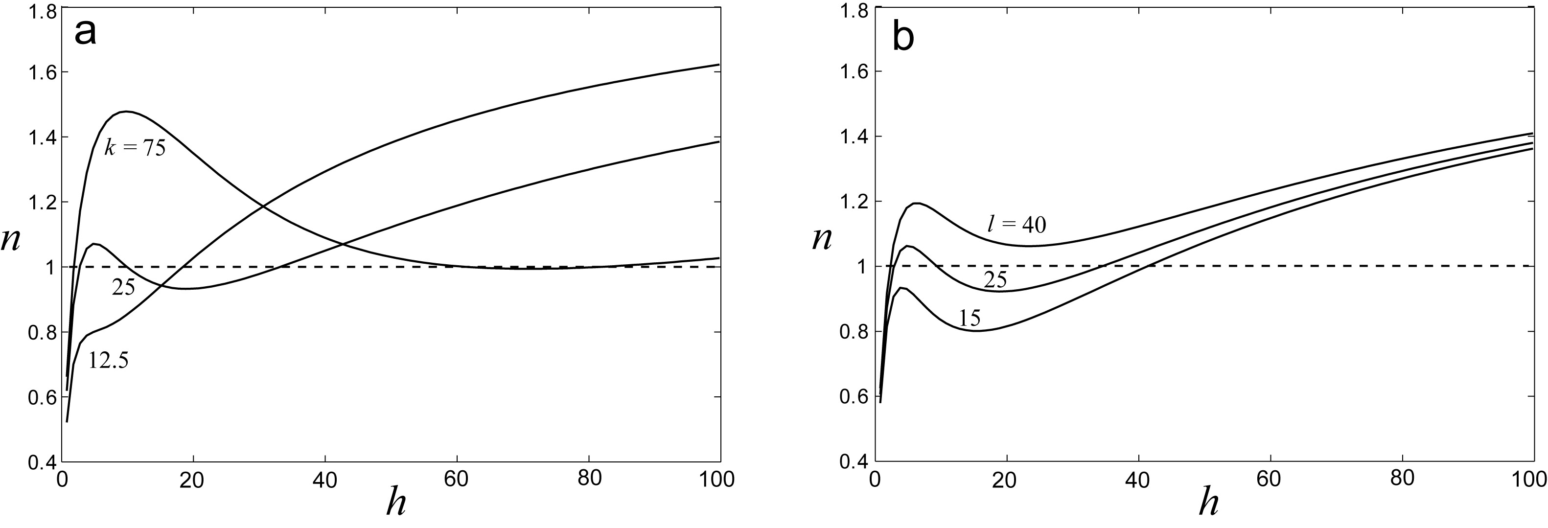
Figure 1: Decay index as a function of height with the value of the parameter $l=25$ and different $k$ (a), and with the value of the parameter $k=25$ and different $l$ (b).

2 Equilibrium of an electric current in a two-scale magnetic field

We extend the 2D model of Priest & Forbes (1990) by introducing another dipole at a larger depth, which produces the field of a larger scale above the surface. The additional source is able to create the additional equilibrium point, which may serve as an intermediate metastable state in a two-step eruption of a filament.

If the electric current is directed along the $y$-axis direction at the height $z=h$ within the plane $x=0$ above the surface of the photosphere $z=0$, the magnetic field of the current outside of the current tube is described by the only one component of the vector potential ${\bf A}=\{0,A_{y},0\}$

$$A_{y}^{I}=\frac{I}{c}[\log\left(x^{2}+(z+h)^{2}\right)-\log\left(x^{2}+(z-h)^{2}\right)],$$ (2)

where the influence of the conductive surface is taken into account as usual by introducing the mirror current $-I$.

For the equilibrium of an inverse polarity filament in the corona, the dipolar moments $m_{1}$ and $m_{2}$ of both two-dimensional dipoles should be directed opposite to the $x$-axis. Their vector potential may be written as

$$A_{y}^{m}=-m_{1}\frac{z+d_{1}}{x^{2}+(z+d_{1})^{2}}-m_{2}\frac{z+d_{2}}{x^{2}+(z+d_{2})^{2}},$$ (3)

where $d_{1}$ and $d_{2}$ are depths of the dipoles below the photosphere. Both dipoles are located also in the plane $x=0$. Then the horizontal component of the force acting on the current tube vanishes according the symmetry, while the vertical component (per unit length) is (van Tend & Kuperus, 1978; Molodenskii & Filippov, 1987; Priest & Forbes, 1990)

$$F_{z}(h)=\frac{I^{2}}{c^{2}h}-B_{x}^{m}(h)\frac{I}{c}-Mg,$$ (4)

where $M$ is the mass of the tube per unit length, $g$ is the free fall acceleration,

$$B_{x}^{m}(z)=-\frac{\partial A_{y}^{m}}{\partial z}.$$ (5)

Equilibrium is achieved at any given height $h$ with the value of the current as

$$I_{0}=c\left(\frac{B_{x}^{m}h}{2}\pm\sqrt{\frac{{B_{x}^{m}}^{2}h^{2}}{4}+Mgh}\right),$$ (6)

The sign (–) before the square root corresponds to a normal polarity filament, not interesting for our study. To solve Equation (4) with the zero left side analytically relative $h$ is not so easy even neglecting the last gravitational term, since we have quartic equation. We may expect, however, that there are two critical heights in this field, each of them corresponding to the scale of the field of each source $m_{1}$ and $m_{2}$.

It was shown (van Tend & Kuperus, 1978; Filippov & Den, 2000, 2001) that a constant straight linear current becomes unstable when the decay index of the background field exceeds unit:

$$n=-\frac{\partial\ln B_{x}}{\partial\ln h}>1.$$ (7)

In the field of a single dipole $m$, the decay index $n$ changes with height $h$ as

$$n(h)=\frac{2h}{h+d}.$$ (8)

For two dipoles (3) it is equal to

$$n(h^{\prime})=2\frac{\left(\frac{h^{\prime}+k}{h^{\prime}+1}\right)^{3}+l}{\left(\frac{h^{\prime}+k}{h^{\prime}+1}\right)^{2}+l}\frac{h^{\prime}}{h^{\prime}+k},$$ (9)

where $h^{\prime}=h/d_{1}$, $k=d_{2}/d_{1}$, $l=m_{2}/m_{1}$. Since it is difficult to solve the equation

$$n(h^{\prime})=1$$ (10)

analytically, we will analyze the right part of Equation (9) numerically in order to choose parameters $k$ and $l$ providing multiple solution of Equation (10).

Figure 1 shows the dependence of the decay index described by Equation (9) on height with different values of the parameters $k$ and $l$. When $k$ is relatively small, the dependence is monotonic, and Equation (10) has only unique solution (Fig. 1a). When $k$ is too large, the curve has extremums but it crosses the line $n=1$ only one time at a low height. Thus we choose $k=25$, which provides three distinct roots of Equation (10). Similarly, we choose the value of the parameter $l=25$ (Fig. 1b). Then we set all dimensionless parameters of the model as $m_{1}=-1,m_{2}=-25,d_{1}=2,d_{2}=50,M=10^{-7},g=30$. Our intention is to describe the equilibrium of a flux rope in the solar corona at a height of about 20 Mm in a magnetic field of about 10 gauss with the gravity force of about 1% of the Lorenz force. This gives that the dimensionless units correspond to: length - 10 Mm, time - $10^{3}$ s, mass - $10^{12}$ g, magnetic induction - 1 gauss. Figure 2 shows the field lines of the model with the equilibrium electric current (6) at the height of 1.5. The field lines are represented by isocontoures of the condition $A_{y}^{I}+A_{y}^{m}=const$.

Figure 3 shows the value of the equilibrium electric current $I_{0}$ as a function of height according to Equation (6). Crossings of the curve with horizontal lines determine equilibrium heights. There are intervals of current values where four, two or no equilibrium positions exist. Crossings with rising parts of the curve correspond to the stable equilibrium; crossings with descending parts correspond to the unstable equilibrium. Two maxima of the curve, at $h\approx 3$ and $h\approx 35$, indicate the places where catastrophic losses of equilibrium can happen. They are two critical heights in the model. As it is seen in Fig. 3, the value of the critical current at the lower point is a little smaller than the critical current at the higher point.

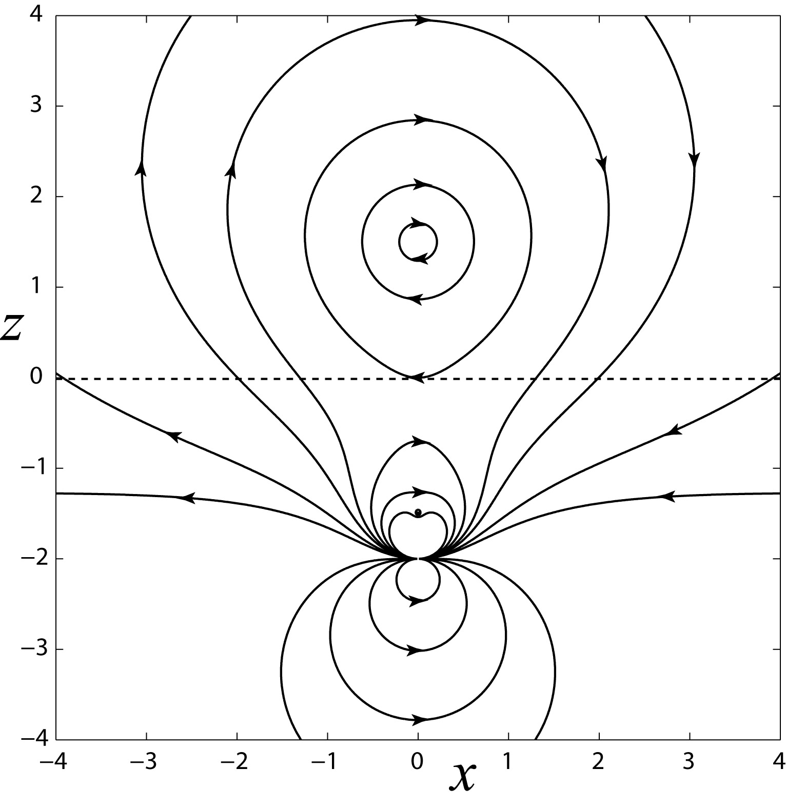
Figure 2: Magnetic field lines of the model with the equilibrium electric current at the height of 1.5.

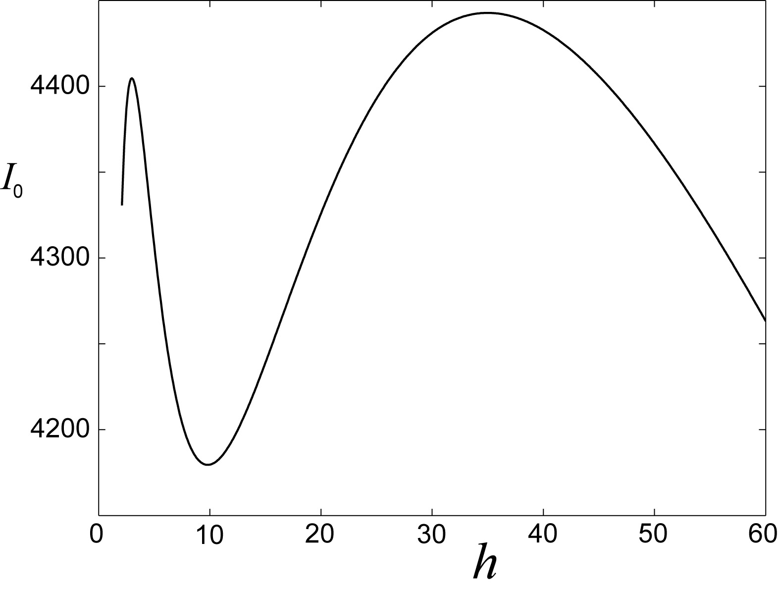
Figure 3: Value of the equilibrium electric current $I_{0}$ as a function of height according to Equation (6).

3 Dynamics of an electric current in the two-scale magnetic field

Let us consider the equation of motion of the current tube in the two-scale magnetic field:

$$M\frac{d^{2}h}{dt^{2}}=F_{z}(h)-\eta\frac{dh}{dt},$$ (11)

where $\eta$ is the coefficient of artificial dissipation (viscosity) introduced in order to avoid long oscillations of the tube. We solve Equation (11) numerically using MATLAB solver ’ode45’ based on an explicit Runge-Kutta formula. Figure 4 shows the relaxation of the tube after small disturbance near the equilibrium position at $h=1.5$. The value of $\eta$ is chosen as $10^{-6}$, which means that the decelerating force at the speed of 1000 km s^-1 is about 1% of the Lorenz force.

The presence of the additional dipole leads to the change of the critical height for the instability from $h_{c}=2$ to $h_{c}\approx 3$. We then put the current tube a little bit lower the critical height and change the both dipolar moments as

$$m_{i}={m_{0}}_{i}\exp\left(-\frac{t^{2}}{\tau^{2}}\right),$$ (12)

with $\tau=10^{3}$ in order to analyze the eruption of the tube. For finite displacements of the current tube we should take into account the changes of the current due to inductance. Priest & Forbes (1990) considered several possibilities to determine current $I$ as a function of $h$ (or $t$).

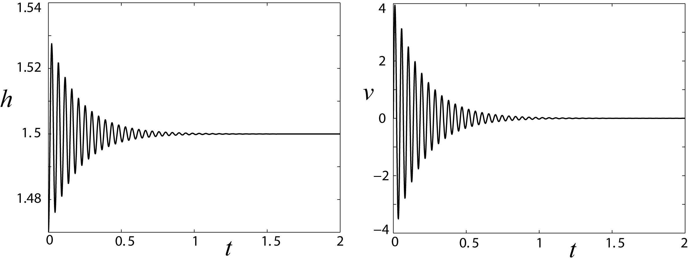
Figure 4: Relaxation of the tube after small disturbance near the equilibrium position at $h=1.5$.

3.1 Constant current

The simplest assumption is $I=const$. Priest & Forbes (1990) decided this case not the most realistic because it needs the source of energy to support the constancy of the current. However, in a case of a partial eruption, when only some section of the long flux rope is moving, the large self-inductance of the circuit can easily support the current to be nearly constant.

Figure 5: Height-time (left) and velocity-time (right) plots of the dynamics of the tube with the constant current.

Figure 5 shows the dynamics of the tube with the constant current starting from the point $h_{0}=2.95$ close to the critical height. After slow rising due to the decreasing the background field, the tube erupts very rapidly at $t=5$ but then decelerates and stops at the height of $h=28$. The tube stays approximately at this height, slowly rising again till to $t=80$. Then the next eruption happens.

The critical height in the field of a single dipole is $h_{c}=d$, while the critical value of the current is

$$I_{c}=\frac{cm}{4d}.$$ (13)

The presence of another dipole raises the critical height in the smaller-scale field from $h_{c}=2$ to $h_{c}\approx 3$ and lowers the critical height in the greater-scale field from $h_{c}=50$ to $h_{c}\approx 30$. Since we have chosen in our model $m_{1}/d_{1}=m_{2}/d_{2}$, the values of the critical current according Equation (13) are equal in both separate fields. In the total field, the critical current value at the higher critical height is a little higher than the critical current at the lower critical height. That is why the tube is able to stop at the intermediate height of $h\approx 30$ and to start the next eruption after the decrease of the background field by about 1%.

3.2 Constant magnetic twist

If we consider the cylindrical tube as a part of a rising three-dimensional loop with the ends anchored in the photosphere, a reasonable approximation is the constant net twist along the tube. Priest & Forbes (1990) showed that this condition leads to the inversion dependence of the current on height

$$I=I_{0}\frac{h_{0}}{h},$$ (14)

where $I_{0}$ is the initial current and $h_{0}$ is the initial height. Eruption becomes impossible under this condition because the equilibrium is stable at any height because the repulsive force (the first term in the right part of Equation (4)) decreases with height faster ($\sim h^{-3}$) than the attractive force (the second term, $\sim h^{-1}(h+d)^{-2}$) even neglecting the gravity.

3.3 Constant magnetic flux

A reasonable condition for determining $I$ is to fix the magnetic flux between the photosphere and the flux tube. Thanks to the translational symmetry the flux is determined by the vector potential

$$\Phi=A_{y}(0)-A_{y}(h-r_{0}),$$ (15)

where $r_{0}$ is the radius of the flux tube. Using Equations (2)-(3) and taking into account that $r_{0}\ll h$ we have

$$\Phi=-\frac{2I}{c}\log\frac{2h}{r_{0}}-m_{1}\frac{h}{d_{1}(d_{1}+h)}-m_{2}\frac{h}{d_{2}(d_{2}+h)}.$$ (16)

The condition $\Phi=const$ determines the dependence of the current value $I$ on height from Equation (16), if we specify the radius of the flux tube $r_{0}$. Figure 5 shows different vertical profiles of the current under various conditions. The lowest curve corresponds to the constant magnetic twist. Two other descending curves show changes of the current in the tube with a constant radius $r_{0}=0.01h_{0}$ and $r_{0}=0.001h_{0}$. Two upper curves correspond to the tubes with the same initial radii but linearly expanding with height. The smaller the tube radius, the weaker the dependence of the current with height.

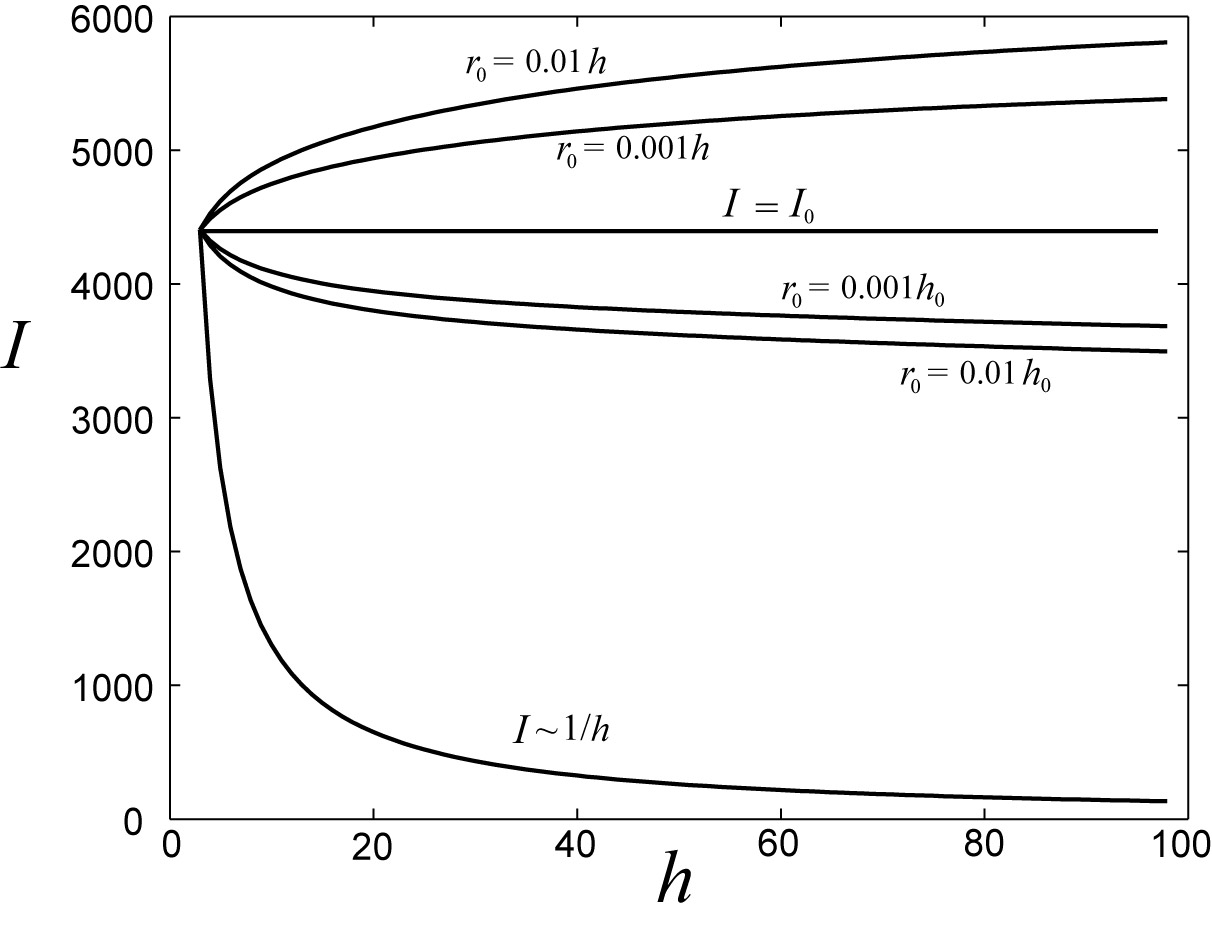
Figure 6: Electric current as a function of height under different conditions.

3.3.1 Constant magnetic flux-tube radius

The condition of the constant magnetic flux between the photosphere and the magnetic flux tube with a constant radius leads to decreasing of the current with height (Fig. 5). Figure 7 shows the rise of the tube of the constant radius $r_{0}=0.001h_{0}$ from the equilibrium position $h_{0}=2.95$, while Figure 8 corresponds to the radius $r_{0}=0.01h_{0}$. In both cases, eruptions start at later time and a larger height than in Fig. 5 since the current is decreasing with height. We see the two-step eruption similar to Fig. 5, but the jump of the tube in the first step is smaller (from $h\approx 3$ to $h\approx 8$) in Fig. 7 and very smooth in Fig. 8. The second-step eruption starts at $t\approx 450$ and $t\approx 550$, respectively. Velocities are lower than in Fig. 5 in the whole event, with the first peak lower than the second one in contrast to Fig. 5. Especially slow is the first eruption in Fig. 8.

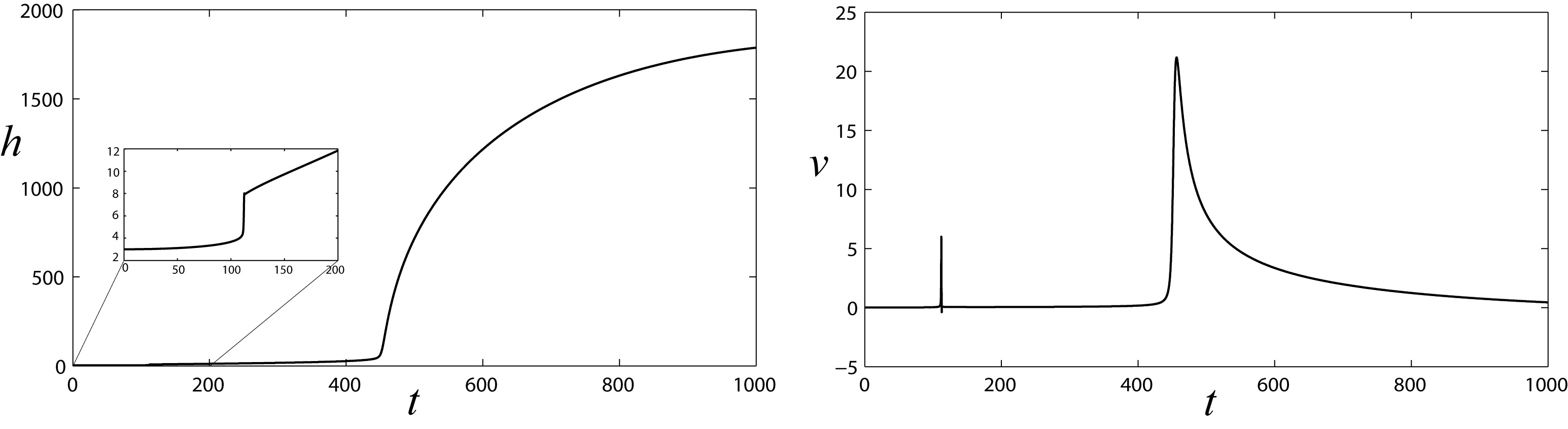
Figure 7: Height-time (left) and velocity-time (right) plots of the dynamics of the tube with the constant radius $r_{0}=0.001h_{0}$.

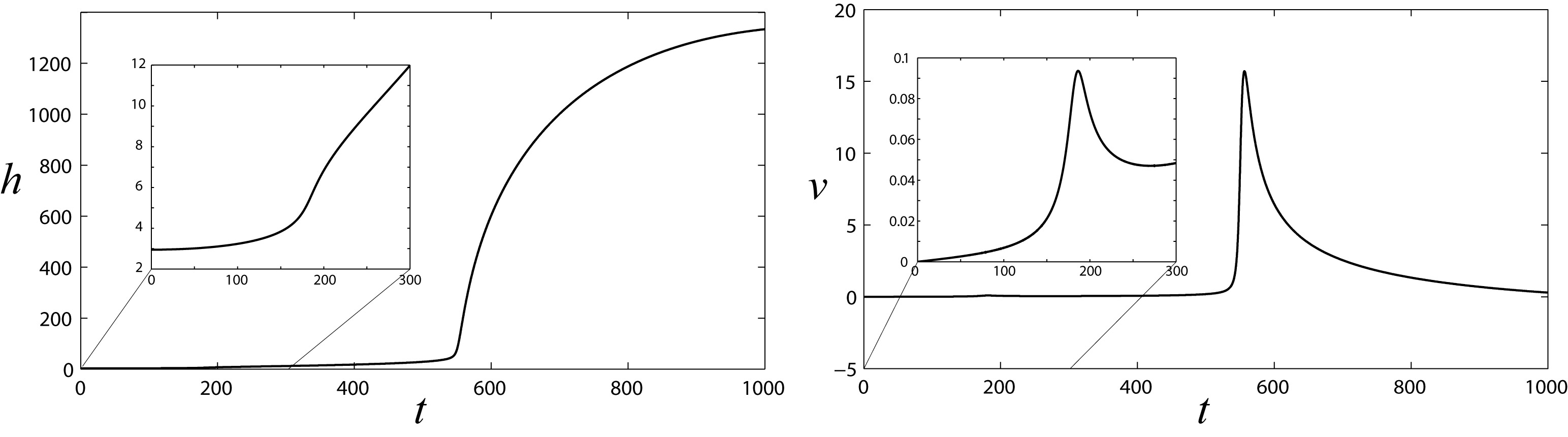
Figure 8: The same as in Figure 7 with the radius $r_{0}=0.01h_{0}$.

3.3.2 Expanding flux-tube

If the radius of the tube expands linearly with height, the current slowly increases with height (Fig. 6). Figure 9 shows the dynamics of the tube with $r_{0}=0.01h$ and $r_{0}=0.001h$ from the equilibrium position $h_{0}=2.95$. The eruption starts violently at $t\approx 0.5$ and does not show the two-step scenario. The tube obtains too high velocity, and the current increases too much for obtaining a higher equilibrium position. It is possible to put the tube at the higher equilibrium point on the rising section of the equilibrium curve in Fig. 3, but the eruption in this case is also a one-step eruption in the larger-scale field.

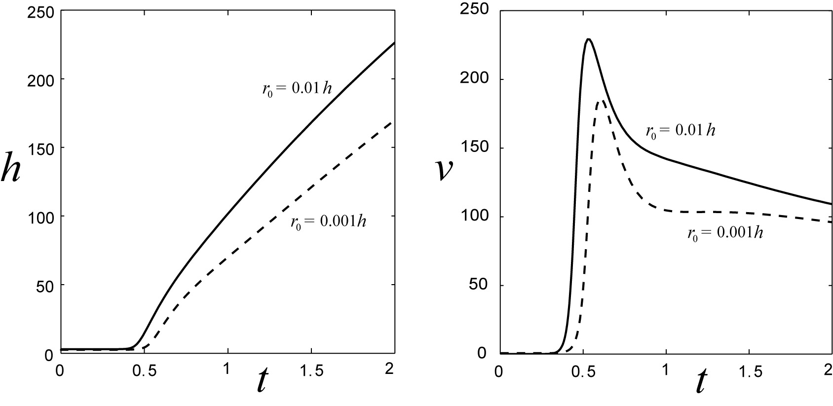
Figure 9: Height-time (left) and velocity-time (right) plots of the dynamics of the tube with the linearly increasing radius $r_{0}=0.001h$ (solid lines) and $r_{0}=0.01h$ (dashed lines).

4 Discussion and Conclusions

We analyzed a possibility of two-step eruptions using a simple 2D model of a twisted flux tube equilibrium in the two-scale coronal magnetic field. This field is created in the model by two 2D dipoles at different depths below the photosphere. We chose parameters of the dipoles in order to have four equilibrium positions for some values of the electric current within the flux tube. Two of them are stable and the other two are unstable. There are two values of the current when a sudden loss of equilibrium happens. Each critical value of the current corresponds to the critical height of the current above the photosphere. We tried to choose the parameters so that the critical heights are quite different but the critical current values are similar. Then, if the coronal field slowly decreases, the tube erupts starting from the lowest critical height. The following evolution of the tube depends on changes of the electric current within it. Owing to induction under different assumptions, it may increase, decrease or to be constant (Fig. 6). If some dissipation is present in the system, the tube can stop at the height between the two critical heights. After rather short time spent in the metastable state, the tube can erupt again from the higher critical height. Thus, the model shows possibility of the two-step eruption under reasonable conditions.

We can compare the vertical profile of the decay index in the model (Fig. 1) with the real distribution of the decay index in the region that produced the two-step eruption (Gosain et al., 2016) (Gosain et al. 2016). Figure 10 shows the distribution of the decay index $n$ calculated in a potential-field approximation on the basis of SDO/HMI magnetogram (the Helioseismic and Mangetic Imager (HMI) (Schou et al., 2012) onboard Solar Dynamics Observatory (SDO)) on 2011 October 18 at 00 UT in the horizontal plane at the height of 70 Mm and along the vertical line above the pre-eruptive position of the filament. The vertical profile has the similar shape as shown in Fig. 1. There are two zones of stability $(n<1)$: one at low heights $h\lesssim 100$ Mm and the second at heights between 350 and 500 Mm.

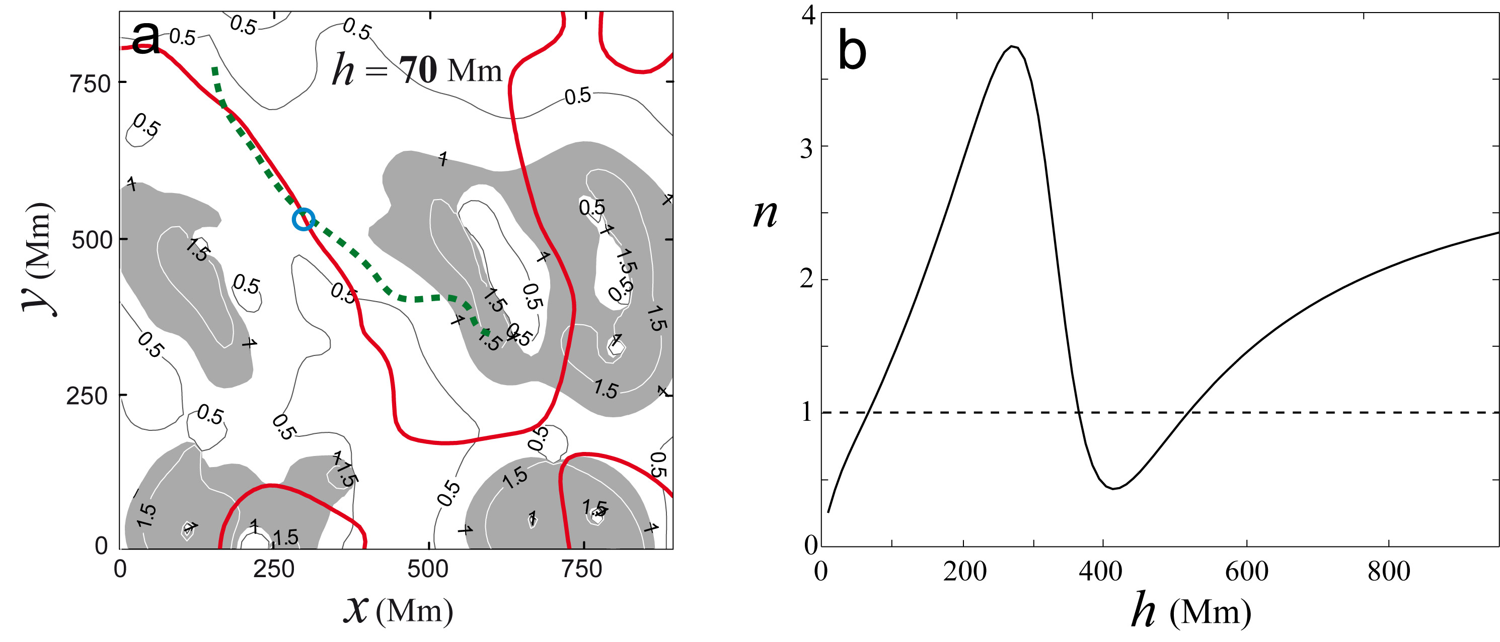
Figure 10: Distribution of the decay index $n$ in the $xy$-plane at the height of 70 Mm (a) and along the vertical line above the blue circle shown in the left panel (b) calculated in a potential-field approximation on the basis of SDO/HMI magnetogram on 2011 October 18 at 00 UT. The dashed green line indicates the position of the quiescent filament.

The eruption of the quiescent filament, shown by the dashed green line in Fig. 10a, started at about 03:40 UT on 2011 October 21. The initial height of the filament was about 100 Mm, close to the first cross of the curve with the line $n=1$ in Fig. 10b. The filament stopped at the height of about 350 Mm (Gosain et al., 2016), which corresponded to the stability zone $(n<1)$ in Fig. 10b. While most of the filament material drained back to the chromosphere shortly after it had stopped, the faint coronal structure was already recognizable before the filament started to ascend again at about 21 UT, more than 17 hours after the start of the first step. The second-step eruption might start near the upper border of the zone of stability at the height of about 500 Mm (Fig. 10b). Thus, the scenario of the event on 2011 October 21 is very similar to the predictions of our model. The two-step eruption owes to the special distribution of the photospheric magnetic field in the region, which manifests itself in owes its existence to the special distribution of the photospheric magnetic field in the region, which manifests itself in the non-monotonic behavior of the decay index in the corona.

An understanding of mechanisms of the two-step eruptions is significant for the perception of the whole picture of solar eruptive events and space weather implications. The large delay of a CME after the filament eruption start may influence on correlation statistics between the two manifestations of an eruption. For the on-disc events that result in faint halo CMEs, estimations of a CME arrival to the Earth on the basis of observations of filament activations may be not very precise. The structure of the coronal magnetic field influences essentially both on the time profile of the filament ascending and its trajectory in the corona.

References

- Alexander et al. (2006) Alexander D., Liu R., Gilbert H. R., 2006, ApJ, 653, 719
- Aulanier et al. (2010) Aulanier G., Török T., Démoulin P., DeLuca E. E., 2010, ApJ, 708, 314
- Bateman (1978) Bateman G., 1978, MHD instabilities
- Byrne et al. (2014) Byrne J. P., Morgan H., Seaton D. B., Bain H. M., Habbal S. R., 2014, Sol. Phys., 289, 4545
- Chandra et al. (2017) Chandra R., Filippov B., Joshi R., Schmieder B., 2017, Sol. Phys., 292, 81
- Cheng et al. (2014) Cheng X., et al., 2014, ApJ, 780, 28
- Dasso et al. (2007) Dasso S., Nakwacki M. S., Démoulin P., Mandrini C. H., 2007, Sol. Phys., 244, 115
- DeVore & Antiochos (2000) DeVore C. R., Antiochos S. K., 2000, ApJ, 539, 954
- Démoulin & Aulanier (2010) Démoulin P., Aulanier G., 2010, ApJ, 718, 1388
- Filippov (2013) Filippov B., 2013, ApJ, 773, 10
- Filippov & Den (2000) Filippov B. P., Den O. G., 2000, Astronomy Letters, 26, 322
- Filippov & Den (2001) Filippov B. P., Den O. G., 2001, J. Geophys. Res., 106, 25177
- Filippov & Zagnetko (2008) Filippov B., Zagnetko A., 2008, Journal of Atmospheric and Solar-Terrestrial Physics, 70, 614
- Filippov et al. (2014) Filippov B. P., Martsenyuk O. V., Den O. E., Platov Y. V., 2014, Astronomy Reports, 58, 928
- Forbes & Isenberg (1991) Forbes T. G., Isenberg P. A., 1991, ApJ, 373, 294
- Forbes & Priest (1995) Forbes T. G., Priest E. R., 1995, ApJ, 446, 377
- Gary & Moore (2004) Gary G. A., Moore R. L., 2004, ApJ, 611, 545
- Gibson (2015) Gibson S., 2015, in Vial J.-C., Engvold O., eds, Astrophysics and Space Science Library Vol. 415, Solar Prominences. p. 323 (arXiv:1702.02214), doi:10.1007/978-3-319-10416-4_13
- Gibson & Fan (2006) Gibson S. E., Fan Y., 2006, Journal of Geophysical Research (Space Physics), 111, A12103
- Gosain et al. (2016) Gosain S., Filippov B., Ajor Maurya R., Chandra R., 2016, ApJ, 821, 85
- Holman & Foord (2015) Holman G. D., Foord A., 2015, ApJ, 804, 108
- Isenberg et al. (1993) Isenberg P. A., Forbes T. G., Demoulin P., 1993, ApJ, 417, 368
- Ji et al. (2003) Ji H., Wang H., Schmahl E. J., Moon Y.-J., Jiang Y., 2003, ApJ, 595, L135
- Joshi & Srivastava (2011) Joshi A. D., Srivastava N., 2011, ApJ, 730, 104
- Joshi et al. (2014) Joshi N. C., Srivastava A. K., Filippov B., Kayshap P., Uddin W., Chandra R., Prasad Choudhary D., Dwivedi B. N., 2014, ApJ, 787, 11
- Kliem & Török (2006) Kliem B., Török T., 2006, Physical Review Letters, 96, 255002
- Kliem et al. (2014) Kliem B., Török T., Titov V. S., Lionello R., Linker J. A., Liu R., Liu C., Wang H., 2014, ApJ, 792, 107
- Kuridze et al. (2013) Kuridze D., Mathioudakis M., Kowalski A. F., Keys P. H., Jess D. B., Balasubramaniam K. S., Keenan F. P., 2013, A&A, 552, A55
- Kushwaha et al. (2015) Kushwaha U., Joshi B., Veronig A. M., Moon Y.-J., 2015, ApJ, 807, 101
- Lepping et al. (1990) Lepping R. P., Burlaga L. F., Jones J. A., 1990, J. Geophys. Res., 95, 11957
- Lin & van Ballegooijen (2002) Lin J., van Ballegooijen A. A., 2002, ApJ, 576, 485
- Lin et al. (1998) Lin J., Forbes T. G., Isenberg P. A., Demoulin P., 1998, ApJ, 504, 1006
- Longcope & Forbes (2014) Longcope D. W., Forbes T. G., 2014, Sol. Phys., 289, 2091
- Martin (1998) Martin S. F., 1998, in Webb D. F., Schmieder B., Rust D. M., eds, Astronomical Society of the Pacific Conference Series Vol. 150, IAU Colloq. 167: New Perspectives on Solar Prominences. p. 419
- Molodenskii & Filippov (1987) Molodenskii M. M., Filippov B. P., 1987, Soviet Ast., 31, 564
- Panasenco et al. (2014) Panasenco O., Martin S. F., Velli M., 2014, Sol. Phys., 289, 603
- Patsourakos et al. (2013) Patsourakos S., Vourlidas A., Stenborg G., 2013, ApJ, 764, 125
- Priest & Forbes (1990) Priest E. R., Forbes T. G., 1990, Sol. Phys., 126, 319
- Schmieder et al. (2013) Schmieder B., Démoulin P., Aulanier G., 2013, Advances in Space Research, 51, 1967
- Schou et al. (2012) Schou J., et al., 2012, Sol. Phys., 275, 229
- Shafranov (1966) Shafranov V. D., 1966, Reviews of Plasma Physics, 2, 103
- Török & Kliem (2005) Török T., Kliem B., 2005, ApJ, 630, L97
- Wang et al. (2016) Wang R., Liu Y. D., Zimovets I., Hu H., Dai X., Yang Z., 2016, ApJ, 827, L12
- Zhang (2013) Zhang Y. Z., 2013, ApJ, 777, 52
- van Tend & Kuperus (1978) van Tend W., Kuperus M., 1978, Sol. Phys., 59, 115