Quantum vacuum polarization around a Reissner-Nordström black hole in five dimensions

Abstract

WKB approximation methods are applied to the case of a massive scalar field around a five-dimensional Reissner-Nordström black hole. The divergences are explicitly isolated and the cancellation against the Schwinger-DeWitt counterterms are proven. The resulting finite quantity is evaluated for different values of the free parameters, namely the black hole mass and charge, and the scalar field mass. We thus extend our previous results on quantum vacuum polarization effects for uncharged asymptotically flat higher-dimensional black holes to electrically charged black holes.

I Introduction

In Flachi:2016bwr we have adapted the WKB method to higher-dimensional Schwarzschild black holes and explicitly calculated the scalar vacuum polarization for the case of five, i.e., (4+1), dimensions everywhere outside the horizon. Other works that have studied vacuum polarization in higher-dimensions are Frolov:1989rv in which the five-dimensional case is also treated, Shiraishi:1993ti in which odd-dimensional anti-de Sitter spacetime is considered, Decanini:2005eg ; Thompson:2008bk in which renormalization in higher-dimensions is developed with care, Breen:2015hwa which studied vacuum polarization on branes, and Breen:2016 ; Breen:2017 in which scalar vacuum polarization, using a mode-sum regularization prescription, is computed for higher-dimensional Schwarzschild black holes with explicit results up to 11 dimensions. The initial studies in vacuum polarization in curved spacetimes christensen ; Candelas:1980zt ; Candelas:1984pg ; Fawcett:1983dk ; Anderson:1989vg focused in four, i.e., (3+1), dimensions and had the aim of improving the understanding of particle production in curved spacetimes and various aspects of black hole evaporation.

Following Flachi:2016bwr , in which higher-dimensional Schwarzschild black holes were studied, here we adapt again the WKB method originally devised in Candelas:1980zt ; Candelas:1984pg to the case of higher-dimensional Reissner-Nordström black holes.

The paper is organized as follows. In Sec. II, we will outline the standard properties of the Green function and its mode-sum decomposition in a five-dimensional spacetime. In Sec. III, the WKB method is used to obtain a truncated approximation of the Green function. In Sec. IV, we use the point-splitting method to renormalize the coincidence limit of the Green function, i.e. the vacuum polarization, regularizing first the summation in the angular modes followed by the energy modes. In Sec. V, we numerically compute the previously calculated renormalized vacuum polarization, providing results for different values of black hole mass, charge and scalar field mass. In Sec. VI, we draw some conclusions.

II Vacuum Polarization in Higher-Dimensions

We are interested in the vacuum polarization $\braket{\phi^{2}(x)}$ of a scalar quantum field, which is given by the coincidence limit of the associated Euclidean Green function $G_{\textrm{E}}$, which satisfies the differential equation

$$\left(\square_{\textrm{E}}-\mu^{2}-\xi R\right)G_{\textrm{E}}(x,x^{\prime})=-{\delta(x-x^{\prime})\over\sqrt{|g|}}\,,$$ (1)

where $\square_{\textrm{E}}$ is the d’Alembertian operator with Euclidean signature, $\mu$ is the scalar field mass, $\xi$ is the coupling constant, $R$ is the spacetime curvature, and $x$ and $x^{\prime}$ are spacetime points.

In this work, we will consider the background to be a five-dimensional black hole described by a five-dimensional metric of the type

$$ds^{2}=-f(r)dt^{2}+{dr^{2}\over f(r)}+r^{2}d\Omega^{2}_{3}\,,$$ (2)

where $t$ and $r$ are the time and radial coordinates, respectively, $d\Omega^{2}_{3}$ represents the line element of a 3-sphere, and $f(r)$ is some function of $r$. We assume that at infinity $f(r)$ goes as $1/r^{2}$ as it should for a five-dimensional spherical asympotically flat spacetime, and we also assume that $f(r)$ contains a horizon at some radius $r_{+}$.

Performing a Wick rotation $t=-i\tau$ on the time coordinate, we obtain the Euclidean metric

$$ds_{\rm E}^{2}=f(r)d\tau^{2}+{dr^{2}\over f(r)}+r^{2}d\Omega^{2}_{3}\,,$$ (3)

which is positive definite everywhere outside the horizon. In order to avoid conical singularities in the Euclidean metric, the coordinate $\tau$ must be periodic with period $\beta$ equal to

$$\beta=4\pi\left({df\over dr}\right)^{-1}_{r=r_{+}}\,.$$ (4)

The quantity $T=\beta^{-1}$ will then be the characteristic temperature of the black hole.

Working in the Hartle-Hawking vacuum state, we may write the finite temperature Euclidean Green function in the mode-sum representation

$$G_{\rm E}(x,x^{\prime})={\alpha\over 4\pi^{3}}\sum^{\infty}_{n=-\infty}e^{i\omega_{n}\Delta\tau}\sum^{\infty}_{l=0}(l+1)C^{(1)}_{l}(\cos\gamma)G_{nl}(r,r^{\prime})$$ (5)

where $\alpha\equiv 2\pi/\beta$, $\Delta\tau=\tau-\tau^{\prime}$, $\omega_{n}\equiv\alpha n$, $\gamma$ is the geodesic distance in the 3-sphere, and $C^{(1)}_{l}(x)$ is a Gengenbauer polynomial. Inserting the mode-sum expansion, Eq. (5), in Eq. (1) leads to the differential equation for the radial Green function

$$\bigg{\{}{d\over dr} \left(r^{3}f(r){d\over dr}\right)-r^{3}\left({\omega^{2}_{n}\over f(r)}+\mu^{2}+\xi R\right)$$

$$\hskip 28.45274pt-l(l+2)r\bigg{\}}G_{nl}(r,r^{\prime})=-\delta(r-r^{\prime})\,.$$ (6)

The solution to Eq. (II) can be expressed in terms of solutions of the corresponding homogeneous equation. In particular, if $p_{nl}(r)$ and $q_{nl}(r)$ are solutions of the homogeneous equation regular at the horizon and infinity, respectively, then the radial Green function can be written as

$$G_{nl}(r,r^{\prime})=C_{nl}\,p_{nl}(r_{<})q_{nl}(r_{>})$$ (7)

where $r_{<}$ and $r_{>}$ denote the largest and the smallest values of the set $\{r,r^{\prime}\}$. The quantity $C_{nl}$ is a normalization constant, given by

$$C_{nl}=-{1\over r^{3}f(r)}{1\over\mathcal{W}(p_{nl}(r),q_{nl}(r))}$$ (8)

where ${\mathcal{W}}(p,q)$ is the Wronskian of the two functions.

We now want to find the solution of Eq. (II). We will first present the approximate limiting solutions at infinity and at the horizon and then we develop the general solution. The limiting solutions serve as boundary conditions for the general solution. In particular they are useful for numerical calculations checking.

III WKB approximation

III.1 Near-infinity and near-horizon solutions

The form of $p_{nl}$ and $q_{nl}$ of the Green function in Eq. (7), solution of Eq. (II), can be obtained by expressing the homogeneous equation in two limits, namely, the near-infinity limit and the near-horizon limit.

Starting with the near-infinity limit, i.e., the large $r$ limit, the homogeneous equation of Eq. (II) becomes

$$\left\{{d^{2}\over dr^{2}}+{3\over r}{d\over dr}-(\omega^{2}_{n}+\mu^{2}+\xi R)\right\}q_{nl}(r)=0\,,$$ (9)

the solution of which, regular at infinity, is of the form

$$q_{nl}(r)\sim r^{-3/2}e^{-r\sqrt{\omega^{2}_{n}+\mu^{2}+\xi R}}\,.$$ (10)

The near-horizon limit may be obtained by using the tortoise coordinate $r_{*}$, defined through $dr_{*}={dr\over f(r)}$, in terms of which, in the near-horizon limit and for $n\neq 0$, the homogeneous equation of Eq. (II) becomes

$$\left({d^{2}\over dr^{2}_{*}}-\omega^{2}_{n}\right)p_{nl}(r)=0\,.$$ (11)

The solution of Eq. (11), regular at the horizon, is given by

$$p_{nl}(r)\sim{e^{-\omega_{n}r_{*}}\over r}\,.$$ (12)

In the case $n=0$, the homogeneous equation of Eq. (II), in the near-horizon limit, becomes ${d\over dr}(\ln p_{0l}(r))={1\over f^{\prime}(r)}\left({l(l+2)\over r^{2}}+\mu^{2}+\xi R\right)$, the solution of which goes as

$$p_{0l}(r)\sim\exp\left\{\int^{r}_{r_{+}}\left({l(l+2)\over u^{2}}+\mu^{2}+\xi R\right){du\over f^{\prime}(u)}\right\}\,.$$ (13)

These limiting solutions will be especially important when performing numerical computations, since they will provide the boundary conditions necessary to solve Eq. (II) numerically.

III.2 WKB general solution

We shall now display a general solution of Eq. (II) by following the standard procedure developed in Candelas:1980zt ; Candelas:1984pg , which makes use of a WKB approximation. We begin by using the following ansatz for the solutions of the homogeneous equation for the radial Green function

$$p_{nl}(r) ={1\over\sqrt{r^{3}W(r)}}\exp\left\{+\int^{r}_{r_{+}}{W(u)\over f(u)}\,du\right\}\,,$$ (14)

$$q_{nl}(r) ={1\over\sqrt{r^{3}W(r)}}\exp\left\{-\int^{r}_{r_{+}}{W(u)\over f(u)}\,du\right\}\,,$$ (15)

where $W$ is the WKB function to be determined. The above expressions are chosen specifically to eliminate all sign dependent terms once inserted in the homogeneous equation of Eq. (II), while at the same time satisfying both the near-horizon and large $r$ limits which are going to be calculated below. We will omit the $n$ and $l$ indices in the WKB function $W(r)$ whenever necessary for notational convenience. In the end, we are left with the homogeneous equation

$$W^{2}=\Phi+a_{1}{W^{\prime}\over W}+a_{2}{W^{\prime 2}\over W^{2}}+a_{3}{W^{\prime\prime}\over W}\,,$$ (16)

where

$$\Phi =\left((l+1)^{2}-1\right){f\over r^{2}}+\sigma(r)\,,$$ (17)

$$\sigma =\omega^{2}_{n}+(\mu^{2}+\xi R)f+{3f^{2}\over 4r^{2}}+{3ff^{\prime}\over 2r}\,,$$ (18)

and

$$a_{1}={ff^{\prime}\over 2},\quad a_{2}=-{3\over 4}f^{2},\quad a_{3}={f^{2}\over 2}\,,$$ (19)

where a prime in the functions $W$ and $f$ denotes a derivative with respect to the coordinate $r$. Inserting Eqs. (14) and (15) in Eq. (7), taking the radial coincidence limit and using the fact the Wronskian is given by $\mathcal{W}(p(r),q(r))=-f/(2W)$, we obtain

$$G_{nl}(r,r)={1\over 2r^{3}W_{nl}(r)}$$ (20)

The solution to Eq. (16) can now be expressed iteratively as $W=W_{0}+W_{1}+\cdots$. At zeroth order, for example, we have $W_{0}=\sqrt{\Phi}$. The expansion we are interested in is

$${1\over W}={1\over\sqrt{\Phi}}(1+\delta\Phi+\delta^{2}\Phi+\ldots)$$ (21)

were $\delta^{n}\Phi/\sqrt{\Phi}$ represents the $n$th order WKB correction to $1/W$. For renormalization purposes, we may only be concerned with the first order approximation, for which one can check that

$$\delta\Phi=-{a_{1}\over 4}{\Phi^{\prime}\over\Phi^{2}}+\left({a_{3}-a_{2}\over 8}\right){\Phi^{\prime 2}\over\Phi^{3}}-{a_{3}\over 4}{\Phi^{\prime\prime}\over\Phi^{2}}\,.$$ (22)

We thus obtain the approximated solution $\tilde{W}$ truncated at first order,

$${1\over\tilde{W}}={1+\delta\Phi\over\sqrt{\Phi}}\,,$$ (23)

or, writing explicitly,

$${1\over\tilde{W}} ={1\over\sqrt{\Phi}}+\alpha_{1}{1\over\Phi^{5/2}}+\alpha_{2}{(l+1)^{2}\over\Phi^{5/2}}$$

$$\hskip 14.22636pt+\alpha_{3}{1\over\Phi^{7/2}}+\alpha_{4}{(l+1)^{2}\over\Phi^{7/2}}+\alpha_{5}{(l+1)^{4}\over\Phi^{7/2}}\,,$$ (24)

with

$$\alpha_{1} =\frac{r\left((a_{1}r-4a_{3})f^{\prime}-a_{1}r^{3}\sigma^{\prime}+a_{3}rf^{\prime\prime}-a_{3}r^{3}\sigma^{\prime\prime}\right)}{4r^{4}}$$

$$\hskip 14.22636pt+\frac{f(6a_{3}-2a_{1}r)}{4r^{4}}\,,$$ (25)

$$\alpha_{2} =\frac{f(2a_{1}r-6a_{3})-r\left((a_{1}r-4a_{3})f^{\prime}+a_{3}rf^{\prime\prime}\right)}{4r^{4}}\,,$$ (26)

$$\alpha_{3} =-\frac{(a_{2}-a_{3})\left(-rf^{\prime}+2f+r^{3}\sigma^{\prime}\right)^{2}}{8r^{6}}\,,$$ (27)

$$\alpha_{4} =-\frac{(a_{2}-a_{3})\left(rf^{\prime}-2f\right)\left(-rf^{\prime}+2f+r^{3}\sigma^{\prime}\right)}{4r^{6}}\,,$$ (28)

$$\alpha_{5} =-\frac{(a_{2}-a_{3})\left(rf^{\prime}-2f\right)^{2}}{8r^{6}}\,.$$ (29)

Taking the spatial coincidence limit, the Euclidean Green function given in Eq. (5) can then be approximated as

$$G_{\rm WKB}(x,x^{\prime})={\alpha\over 8\pi^{3}r^{3}}\sum^{\infty}_{n=-\infty}e^{i\omega_{n}\Delta\tau}\sum^{\infty}_{l=0}{(l+1)^{2}\over\tilde{W}_{nl}(r)}\,.$$ (30)

The Euclidean Green function in Eq. (30) is divergent both in the angular and energy modes, i.e., in the $l$ and $n$ modes, respectively. We take care of this in the following. The divergence in the angular $l$ modes is purely mathematical and can be promptly removed. On the other hand, the divergent terms in the energy $n$ modes are physical and must be canceled by some counterterms in order to obtain a fully renormalized result. First we regularize the $l$ modes and afterward the $n$ modes.

IV Renormalization

IV.1 Regularization in the $l$ modes

The summation in the angular modes for large $l$ will be divergent so long as terms of $(l+1)$ with powers larger than $-1$ are present. Expanding $(l+1)^{2}/\tilde{W}$ for large $(l+1)$, we obtain

$$\mathcal{T}_{l}(r)= {r\over\sqrt{f}}(l+1)+{r\over 32f^{3/2}(l+1)}(-16r^{2}\omega^{2}_{n}+16f$$

$$-4f^{2}-16f\sigma+4rff^{\prime\prime}+r^{2}f^{\prime 2}-4r^{2}ff^{\prime\prime})\,,$$ (31)

which diverges in the final sum of Eq. (30). This divergence is not physical, and can be removed by subtracting the quantity ${\alpha\over 8\pi^{3}r^{3}}\sum^{\infty}_{n=-\infty}e^{i\omega_{n}\Delta\tau}\sum^{\infty}_{l=0}\mathcal{T}_{l}(r)$, from Eq. (30). The term involving $\omega^{2}_{n}$ is irrelevant, since the summation in $n$ will give $\zeta(-2)$, which is zero. This means the dependence of $\mathcal{T}_{l}$ is purely on $l$, and so, ${\alpha\over 8\pi^{3}r^{3}}\sum^{\infty}_{n=-\infty}e^{i\omega_{n}\Delta\tau}\sum^{\infty}_{l=0}\mathcal{T}_{l}(r)$ is a multiple of $\delta(\alpha\Delta\tau)$. Therefore, since $\Delta\tau\neq 0$, we are effectively subtracting 0, canceling the divergent large $l$ behavior in the process. After the subtraction we may take the full coincidence limit, for which the Green function becomes

$$G_{\rm WKB}(x,x)={\alpha\over 8\pi^{3}r^{3}}\sum^{\infty}_{n=-\infty}\sum^{\infty}_{l=0}\left\{{(l+1)^{2}\over\tilde{W}_{nl}}-\mathcal{T}_{l}\right\}\,.$$ (32)

IV.2 Regularization in the $n$ modes

We now proceed to the regularization of the $n$ modes, physically associated to UV divergences. We will isolate the divergent pieces of Eq. (32) and explicitly see that they cancel with the counterterms provided by the point-splitting method developed in christensen .

The Green function (32) can be written as

$$G_{\rm WKB}(x,x)={\alpha\over 8\pi^{3}r^{3}}\left(G_{0}+2\sum^{\infty}_{n=1}G_{n}\right)\,,$$ (33)

where we have defined $G_{n}$ as

$$G_{n}=\sum^{\infty}_{l=0}\left({(l+1)^{2}\over\tilde{W}_{nl}}-\mathcal{T}_{l}\right)$$ (34)

and have made use of the fact that $\sum^{\infty}_{n=-\infty}G_{n}=G_{0}+2\sum^{\infty}_{n=1}G_{n}$. The term $G_{0}$ is finite by construction, so all divergences must be contained within $G_{n}$. In particular, powers of $n$ larger than $-1$ will result in infinity after the summation. To obtain an expression for $G_{n}$, we shall make use of the Abel-Plana sum formula

$$\sum^{\infty}_{l=j}f(l) =\int^{\infty}_{0}{dt\over e^{2\pi t}-1}[f(j+it)-f(j-it)]$$

$$\hskip 14.22636pt+{f(j)\over 2}+\int^{\infty}_{j}f(\tau)\,d\tau\,.$$ (35)

Applying Eq. (IV.2) to Eq. (34) and expanding for large $n$, we arrive at the following divergent part of the Green function

$$G_{\rm div} ={\alpha\over 8\pi^{3}f^{3/2}}\sum^{\infty}_{n=1}\bigg{[}\bigg{(}\mu^{2}f-{f\over r^{2}}+{6\xi f\over r^{2}}+{f^{2}\over r^{2}}-{6\xi f^{2}\over r^{2}}$$

$$+{5ff^{\prime}\over 4r}-{6\xi ff^{\prime}\over r}-{f^{\prime 2}\over 16}+{ff^{\prime\prime}\over 4}-\xi ff^{\prime\prime}\bigg{)}\ln\omega_{n}+\omega^{2}_{n}\ln\omega_{n}\bigg{]}\,.$$ (36)

The divergent terms of the form $1/\omega_{n}$ cancel out, as expected from spacetimes with odd dimensions; see Thompson:2008bk . To obtain a finite renormalized result we should subtract the counterterms given in Eq. (IV.2) from Eq. (32), i.e.,

$$G_{\rm reg}=G_{\rm WKB}-G_{\rm div}\,.$$ (37)

In order to check that Eq. (IV.2) is the correct divergent part we use the generic method devised by Christensen, i.e., the point-slpitting method christensen . Choosing the point split to lie in the $\tau$ coordinate, the geodesic separation $\sigma$ becomes

$$\sigma={f\over 2}\varepsilon^{2}-{ff^{\prime 2}\over 96}\varepsilon^{2}+\mathcal{O}(\varepsilon^{6})\,,$$ (38)

and the Schwinger-DeWitt counterterms are then given by

$$G_{\rm SD} =\lim_{\varepsilon\to 0}\bigg{\{}{1\over 16\pi\sqrt{f}\varepsilon}\left(\left({1\over 6}-\xi\right)R-\mu^{2}-{f^{\prime}\over 4r}+{f^{\prime 2}\over 16f}\right)$$

$$\hskip 19.91692pt+{1\over 8\pi^{2}f^{3/2}\varepsilon^{3}}\bigg{\}}\,.$$ (39)

Now, we must express the counterterms as a sum in energy modes, and in order to do that, we convert the inverse powers of $\varepsilon$ into sums by using the results

$$\lim_{\varepsilon\to 0}{1\over\varepsilon} =-{2\alpha\over\pi}\sum^{\infty}_{n=1}\ln\omega_{n}+\mathcal{O}(\varepsilon)\,,$$ (40)

$$\lim_{\varepsilon\to 0}{1\over\varepsilon^{3}} ={\alpha\over\pi}\sum^{\infty}_{n=1}\omega^{2}_{n}\ln\omega_{n}+\mathcal{O}(\varepsilon)\,,$$ (41)

derived in Flachi:2016bwr . Inserting Eqs. (40) and (41) into Eq. (IV.2), one immediately arrives at Eq. (IV.2), thus confirming its correctness.

V Numerical results for the five-dimensional electrically charged Reissner-Nordström black hole

In obtaining $G_{\rm reg}$ one has made use of the WKB approximation, since $G_{\rm reg}=G_{\rm WKB}-G_{\rm div}$. We want to go a step further and obtain a more exact result. The remainder $\delta G$ between the exact value of the Euclidean Green function $G_{\rm E}$ and the WKB approximated Green function $G_{\rm WKB}$, i.e., $\delta G=G_{\rm E}-G_{\rm WKB}$, is usually ignored because it is considered negligible. However, here, in our numerical calculation, we take care of this remainder $\delta G$. Thus, instead of writing the approximated vacuum polarization expression as usual, $\braket{\phi^{2}(x)}_{\textrm{ren.}}=G_{\rm reg}$, we use the exact value for the fully renormalized vacuum polarization as

$$\braket{\phi^{2}(x)}_{\textrm{ren.}}=G_{\rm reg}+\delta G\,.$$ (42)

The quantity $G_{\rm reg}$ can be evaluated directly using Eq. (37). In the numerical results that follow, we have used the WKB approximation up to second order and calculated numerically the remainder $\delta G$, which is the most computationally demanding term. In the process of numerically calculating the remainder, we used Eqs. (12) and (13) for the first point in the numerical range of the solution (near-horizon limit) and Eq. (10) for the last point (large radius limit). Of course, if we were to increase the order of the WKB approximation in $G_{\rm reg}$, it would reduce the magnitude of the remainder $\delta G$. We have opted to use the WKB approximation up to second order since it in general yields accurate results.

In what follows, we specify that the metric given in Eq. (2) is the metric for a five-dimensional electrically charged Reissner-Nordström black hole, such that $f(r)$ is given by

$$f(r)=1-{2m\over r^{2}}+{q^{2}\over r^{4}}\,,$$ (43)

where $m$ is the mass parameter and $q$ is the electrically charge parameter. The metric function $f(r)$ given in Eq. (43) has an event horizon with radius

$$r_{+}=\left(m+\sqrt{m^{2}-q^{2}}\right)^{1/2}\,.$$ (44)

It has another horizon, the Cauchy horizon, with radius $r_{-}=\left(m-\sqrt{m^{2}-q^{2}}\right)^{1/2}$, but it does not enter into our calculations. In addition, for the function $f(r)$ given in Eq. (43), the inverse Hawking temperature defined in Eq. (4) is

$$\beta={(m+\sqrt{m^{2}-q^{2}})^{5/2}\over(m^{2}-q^{2}+m\sqrt{m^{2}-q^{2}})}\pi\,.$$ (45)

For completeness we remark that the parameters $m$ and $q$ appearing in Eq. (43) are related to the black hole ADM mass $M$ and electrical charge $Q$, through the relations $m={4G_{5}M\over 3\pi}$ and $q^{2}={4\pi\over 3}G_{5}Q^{2}$, respectively, where $G_{5}$ is the gravitational constant for a five-dimensional spacetime.

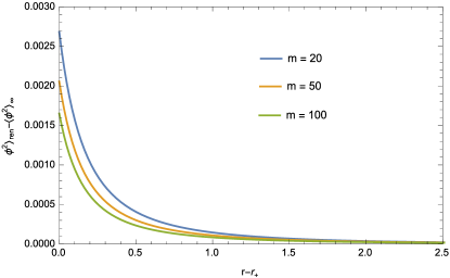
Figure 1: Plots of the vacuum polarization $\braket{\phi^{2}}_{\textrm{ren}}-\braket{\phi^{2}}_{\infty}$ as a function of the coordinate distance from the black hole horizon radius, i.e., $r-r_{+}$, for three black hole masses $m$. The charge and scalar field mass are fixed as $q=10$ and $\mu=0$, respectively.

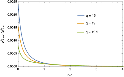
Figure 2: Plots of the vacuum polarization $\braket{\phi^{2}}_{\textrm{ren}}-\braket{\phi^{2}}_{\infty}$ as a function of the coordinate distance from the black hole horizon radius, i.e., $r-r_{+}$, for three black hole charges $q$. The back hole and scalar field masses are fixed as $m=20$ and $\mu=0$, respectively.

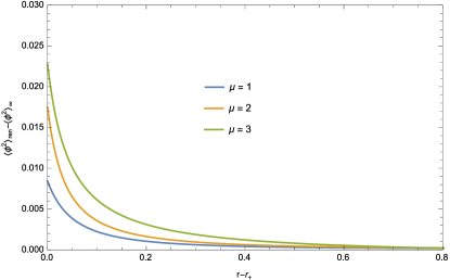
Figure 3: Plots of the vacuum polarization $\braket{\phi^{2}}_{\textrm{ren}}-\braket{\phi^{2}}_{\infty}$ as a function of the coordinate distance from the black hole horizon radius, i.e., $r-r_{+}$, for three scalar field masses $\mu$. The mass and charge of the black hole are fixed as $m=20$ and $q=10$, respectively.

In Figs. 1-3, we plot $\braket{\phi^{2}}_{\textrm{ren}}-\braket{\phi^{2}}_{\infty}$, i.e., the renormalized vacuum polarization normalized to zero at infinity, as a function of the coordinate distance from the five-dimensional Reissner-Nordström black hole horizon radius, i.e., $r-r_{+}$, for three different values of the black hole mass, black hole electric charge, and scalar field mass, respectively. For each parameter choice, we find finite values at the horizon with no problems of convergence. Note that, since we deal with a five-dimensional Reissner-Nordström black hole, the curvature $R$ is identically zero, and so the coupling constant $\xi$ is irrelevant in our calculations. In Fig. 1, we see that the value of the vacuum polarization at the horizon decreases with increasing black hole mass. This is expected, as the black hole temperature decreases and so it is harder to produce excitations in the quantum field. In Fig. 2, the value at the horizon decreases with increasing charge, i.e., as the black hole approaches the extremal limit. This is again expected, as an extremal black hole has zero temperature. In Fig. 3, we see that increasing scalar field mass induces a larger vacuum polarization at the horizon.

VI Conclusions

In this work we have extended our previous results Flachi:2016bwr and calculated the renormalized vacuum polarization for a massive scalar field around a five-dimensional electrically charged black hole. We have followed the standard approach which makes use of the WKB approximation to extract the infinities present both in the angular and energy modes of the mode-sum expanded Green function. We have also compared the explicit divergent part with the Schwinger-DeWitt counterterms to get a fully renormalized result for the vacuum polarization. Terms up to second order were used in the approximation, which provided numerical results illustrating the behavior of the vacuum polarization as a function of the various parameters. A simple understanding of the finer features of the vacuum polarization $\braket{\phi^{2}}_{{\rm ren}}$ in the various cases is difficult due to the complexity of the calculations involved.

VII Acknowledgments

G.Q. acknowledges Fundação para a Ciência e Tecnologia(FCT), (Portugal) through Grant No. SFRH/BD/92583/2013. A.F. acknowledges the MEXT-supported Program, Japan, for the Strategic Research Foundation at Private Universities “Topological Science,” Grant No. S1511006. J.P.S.L. acknowledges FCT for financial support through Project No. UID/FIS/00099/2013 and Grant No. SFRH/BSAB/128455/2017, and Coordenação de Aperfeiçoamento do Pessoal de Nível Superior (CAPES), Brazil, for support within the Programa CSF-PVE, Grant No. 88887.068694/2014-00.

References

- (1) A. Flachi, G. M. Quinta, and J. P. S. Lemos, Black hole quantum vacuum polarization in higher-dimensions, Phys. Rev. D 94, 105001 (2016); arXiv:1609.06794 [gr-qc].
- (2) V. P. Frolov, F. D. Mazzitelli, and J. P. Paz, Quantum effects near multidimensional black holes, Phys. Rev. D 40, 948 (1989).
- (3) K. Shiraishi and T. Maki, Vacuum polarization near asymptotically anti-de Sitter black holes in odd dimensions, Classical Quantum Gravity 11, 1687 (1994).
- (4) Y. Decanini and A. Folacci, Hadamard renormalization of the stress-energy tensor for a quantized scalar field in a general spacetime of arbitrary dimension, Phys. Rev. D 78, 044025 (2008); arXiv:0512118 [gr-qc].
- (5) R. T. Thompson and J. P. S. Lemos, DeWitt-Schwinger renormalization and vacuum polarization in dimensions, Phys. Rev. D 80, 064017 (2009); arXiv:0811.3962 [gr-qc].
- (6) C. Breen, M. Hewitt, A. C. Ottewill, and E. Winstanley, “Vacuum polarization on the brane”, Phys. Rev. D 92, 084039 (2015); arXiv:1507.05026 [gr-qc].
- (7) P. Taylor and C. Breen, A mode-sum prescription for vacuum polarization in odd dimensions, Phys. Rev. D 94, 125024 (2016); arXiv:1609.08166 [gr-qc].
- (8) P. Taylor and C. Breen, A mode-sum prescription for vacuum polarization in even dimensions, Phys. Rev. D 96, 105020 (2017); arXiv:1709.00316 [gr-qc].
- (9) S. M. Christensen, Vacuum expectation value of the stress tensor in an arbitrary curved background: The covariant point-separation method, Phys. Rev. D 14, 2490 (1976).
- (10) P. Candelas, Vacuum polarization in Schwarzschild space-time, Phys. Rev. D 21, 2185 (1980).
- (11) P. Candelas and K. W. Howard, Vacuum in Schwarzschild space-time, Phys. Rev. D 29, 1618 (1984).
- (12) M. S. Fawcett, The energy-momentum tensor near a black hole, Commun. Math. Phys. 89, 103 (1983).
- (13) P. R. Anderson, for massive fields in Schwarzschild space-time, Phys. Rev. D 39, 3785 (1989).