A bivariate polynomial interpolation problem for matrices

Abstract.

In this article, we propose a bivariate polynomial interpolation problem for matrices (BVPIPM), for real matrices of the order $m\times n$. In the process of solving the proposed problem, we establish the existence of a class of $mn$-dimensional bivariate polynomial subspaces (BVPS) in which the BVPIPM always posses a unique solution. Two formulas are presented to construct the respective polynomial maps from the space of real matrices of the order $m\times n$ to two of the particular established BVPS, which satisfy the BVPIPM, by introducing an approach of bivariate polynomial interpolation. Further, we prove that these polynomial maps are isomorphisms. Some numerical examples are also provided to validate and show the applicability of our theoretical findings.

1. Introduction

The finite-order real matrices and polynomials are used in a large scale to solve the computational problems, see [2, 5, 12]. Nowadays, a finite-order real matrix is commonly used data structure to store the complete information of the objects (independent of the contents) in several algorithms and methods of science and engineering. Particularly in image and signal processing [20], computer graphics [14], thermal engineering [19], computer aided design in control systems [7, 13], to name a few. For instance, an image captured by camera can be sampled by a continuous digital image function $f(x,y)$. Digital image functions are used for computerized image processing and represented by finite-order real matrices such that the domain is the region $\left\{(x,y):1\leq x\leq x_{m},1\leq y\leq y_{n}\right\}$, where $x_{m}$, $y_{n}$ are the maximal image natural coordinates in the plane (see [14, 20] for details).

As well, in the case of more than one variable, there is an important relation between the polynomial interpolation and the construction of the polynomial ideals. The bases of polynomial ideals have been used in the development of many ideas in computer algebra and numerical analysis. Some of the related review articles are summarized in [8, 9, 18]. For a specific application, see [15]. Moreover, the surface interpolation provides a crucial and essential contribution in the computer-assisted medical diagnosis and surgical planning through the construction (or reconstruction) of three-dimensional smooth interpolating surfaces from the given (sometimes constructed) data of the images, in medical imaging. The repairing of holes in the skull by generating the three-dimensional smooth interpolating surfaces (using radial basis functions) is discussed in [6].

In general, the polynomials are mostly used to approximate the continuous functions and smooth curves. The simple reason is that they are continuously differentiable, integrable and generate smooth interpolating surfaces with respect to the sampled data. Therefore, the construction of the polynomials in some of the finite-dimensional BVPS, of various total degree, with respect to the given information in form of a finite-order real matrix, can be advantageous in the several stages of analysis (or applications) in science and engineering.

1.1. Preliminaries

Let $\Pi^{d}$ be the $d$-variate polynomial space and $\Pi_{k}^{d}$ be ${k+d\choose{k}}$-dimensional subspace of $\Pi^{d}$, of total degree up to $k$, over the field of real numbers, where $d$ and $k$ are non-negative integers, [18]. Also, let $\mathbb{R}^{m\times n}$ be the space of $m\times n$ real matrices and $({\alpha_{ij}})\in\mathbb{R}^{m\times n}$ represent the matrix $A=({\alpha_{ij}})_{m\times n}$ in $\mathbb{R}^{m\times n}$, [1, 4].

Let $r\in\mathbb{N}$ and $\mathcal{X}=\left\{x_{1},x_{2},\ldots,x_{r}\right\}$ be the sequence of $r$-pairwise disjoint points in $\mathbb{R}^{d}$. For some given subspace $\mathcal{P}\subset\Pi^{d}$ and an associated vector $Y=(y_{1},y_{2},...,y_{r})$ of prescribed real values, find a polynomial $p\in\mathcal{P}$ such that

(1.1) $$\mathcal{X}p=Y,\quad i.e.,\quad p(x_{i})=y_{i}\textrm{ for all }i=1,2,...,r$$

can be read as $d$-variate Lagrange polynomial interpolation problem. The points $x_{i}$, $i=1,2,...$ are called interpolation points or nodes, [9, 17].

Definition 1.1.

[9, 17] The interpolation problem (1.1) with respect to $\mathcal{X}$ is called poised in $\mathcal{P}$, if a polynomial $p\in\mathcal{P}$ exists uniquely such that the condition (1.1) holds for every given choice of $Y$.

Proposition 1.2.

[17] The interpolation problem (1.1) with respect to $\mathcal{X}$ is poised in $\mathcal{P}$, iff

1. $r=\dim(\mathcal{P})$, and

2. the determinant of the sample matrix, $\mathcal{X}\mathcal{B}=\begin{bmatrix}xp:x\in\mathcal{X},p\in\mathcal{B}\end{bmatrix}\in\mathbb{R}^{{\mathcal{X}}\times\mathcal{B}}$, is non-zero for any choice of basis $\mathcal{B}$ of $\mathcal{P}$.

If the interpolation problem (1.1) with respect to $\mathcal{X}$ is poised in $\mathcal{P}$ then $\mathcal{P}$ is known as an interpolation space or correct space. It should be noted that the remaining part of work in this article focuses on bivariate case only, i.e., $d=2$.

Proposed Problem: For some given $m,n\in\mathbb{N}$ and a subspace $\mathcal{H}$ of $\Pi^{2}$, if we consider the problem to find the matrix $(a_{ij})\in\mathbb{R}^{m\times n}$, such that $a_{ij}=\wp(i,j)$ for all $i=1,2,\ldots,m$, $j=1,2,\ldots,n$, where $\wp\in\mathcal{H}$ be a known (or given) polynomial. Then, this problem can be solved easily and the required matrix $\left(\wp(i,j)\right)\in\mathbb{R}^{m\times n}$ can be constructed uniquely. Here, we are proposing the respective converse problem as follows.

$\bullet$ For a given $({\alpha_{ij}})\in\mathbb{R}^{m\times n}$ and subspace $\mathcal{H}$ of $\Pi^{2}$, find a polynomial $\wp\in\mathcal{H}$ with respect to the set $\Xi=\left\{(i,j):i=1,2,\ldots,m,j=1,2,\ldots,n\right\}$, of pair-wise disjoint interpolation points, such that

(*) $$\wp(i,j)={\alpha_{ij}}\quad\forall\;\;i=1,2,\ldots,m,\;j=1,2,\ldots,n$$

is called the BVPIPM.

Remark 1.3.

For any given $({\alpha_{ij}})\in\mathbb{R}^{m\times n}$, the BVPIPM (* ‣ 1.1) with respect to $\Xi$ cannot always be poised in ${k+2}\choose{k}$-dimensional subspace $\Pi_{k}^{2}$, for $k\in\mathbb{N}$, in view of the following facts:

1. If $k=mn-1$, then $mn=\dim\Pi_{mn-1}^{2}$ implies that either $m=0$ or $n=0$ or $m=n=1$.

2. If $k\neq mn-1$ and $mn=\dim\Pi_{k}^{2}$, then the determinant of the associated sample matrix becomes zero, in most of the cases, (see Appendix A).

3. If $k$ is such that $mn\neq\dim\Pi_{k}^{2}$, then the necessity of given nodes (or data points) can not be fulfilled.

The BVPIPM (* ‣ 1.1) is a particular case of the bivariate polynomial interpolation problem with respect to a finite-number of equally spaced interpolation points, proposed by the author Seimatsu Narumi in [16]. Therefore, the BVPIPM (* ‣ 1.1) can always be poised in $\Pi_{m}^{1}\times\Pi_{n}^{1}$, tensor product of two univariate polynomial spaces of dimension $mn$ with total degree $m+n-2$, suggested by the author Narumi in [16]. An overview of related literature is also included in [8]. In spite of this, for $d=2$, the BVPIPM (* ‣ 1.1) is also a particular case of Lagrange polynomial interpolation problem (1.1) with respect to a special set of $r$-pairwise distinct nodes $\Xi$. Due to Kergin interpolation [10], there always exist at least one $r$-dimensional subspace of $\Pi_{r-1}^{d}$ in which the interpolation problem (1.1) with respect to any set of $r$-pairwise distinct nodes in $\mathbb{R}^{d}$ can be poised. Therefore, there may exist more than one $mn$-dimensional subspace of $\Pi^{2}_{mn-1}$ in which the BVPIPM (* ‣ 1.1) with respect to $\Xi$ can always be poised for any given $({\alpha_{ij}})\in\mathbb{R}^{m\times n}$.

The main objective of this article is to establish the existence of some new $mn$-dimensional subspaces of $\Pi_{mn-1}^{2}$, in which the BVPIPM (* ‣ 1.1) with respect to $\Xi$, can always be poised for all $({\alpha_{ij}})\in\mathbb{R}^{m\times n}$. Present some formulas to construct the respective polynomial maps from $\mathbb{R}^{m\times n}$ to the established subspaces, discuss some of the algebraic properties of such polynomial maps such as linearity and invertibility, are the other objectives.

The remaining article is organized in the following manner. Section 2 includes the main results of this article. In section 3, some numerical examples are provided to validate and show the applicability of the results. The concluding remarks are discussed in section 4.

2. Main results

In this section, a class of $mn$-dimensional subspaces of $\Pi_{mn-1}^{2}$ is defined and the existence of these subspaces is established by proving that the BVPIPM (* ‣ 1.1) with respect to $\Xi$ is always poised in them, for all given $({\alpha_{ij}})\in\mathbb{R}^{m\times n}$. Some formulas are also presented to construct the respective polynomial maps from $\mathbb{R}^{m\times n}$ to two of the particular established subspaces, that satisfy the BVPIPM (* ‣ 1.1) with respect to $\Xi$. Moreover, it is proved that these polynomial maps are isomorphisms.

Definition 2.1.

For some real scalars $\alpha$ and $\beta$, let ${}_{\alpha}^{\beta}\Pi_{m,n}^{2}$ be the space of bivariate polynomials with real coefficients, of total degree up to $mn-1$, such that, if $P\in{{}_{\alpha}^{\beta}\Pi_{m,n}^{2}}$, then

(2.1) $$P(x,y)=\sum_{k=0}^{mn-1}{{\lambda_{k}}(\alpha x+\beta y)^{k}}.$$

Theorem 2.2.

The space ${}_{\alpha}^{\beta}\Pi_{m,n}^{2}$ is an $mn$-dimensional subspace of $\Pi_{mn-1}^{2}$.

Remark 2.3.

The set $\left\{1,(\alpha x+\beta y),(\alpha x+\beta y)^{2},\ldots,(\alpha x+\beta y)^{mn-1}\right\}$ is a basis of ${}_{n}^{1}\Pi_{m,n}^{2}$.

Theorem 2.4.

For every $({\alpha_{ij}})\in\mathbb{R}^{m\times n}$, there exists a unique $P\in{{}_{\alpha}^{\beta}\Pi_{m,n}^{2}}$ which satisfy the BVPIPM (* ‣ 1.1) with respect to $\Xi$, such that the pair $(\alpha,\beta)$ satisfy the condition,

(2.2) $$\alpha i_{1}+\beta j_{1}\neq\alpha i_{2}+\beta j_{2}\textrm{ for all }i_{1}\neq i_{2}\textrm{ and }j_{1}\neq j_{2}.$$

Proof.

Let $P\in{{}_{n}^{1}\Pi_{m,n}^{2}}$ be the polynomial that satisfy the BVPIPM (* ‣ 1.1) with respect to $\Xi$ and is given as

(2.3) $$P(x,y)=\sum_{k=0}^{mn-1}{{\lambda_{k}}(\alpha x+\beta y)^{k}}.$$

Therefore, we can write

(2.4) $${\alpha_{ij}}=\sum_{k=0}^{mn-1}{{\lambda_{k}}(\alpha x+\beta y)^{k}}\textrm{ for all }i=1,2,\ldots,m,\;\;j=1,2,\ldots,n,$$

where $\lambda_{k}$, $k=1,2,\ldots,mn-1$ are some coefficients. Thus, the coefficients must satisfy the system of equations of the form

(2.5) $${\Lambda}X=\mu,$$

where, $X={\begin{pmatrix}\lambda_{0}~{}\lambda_{1}~{}\ldots~{}\lambda_{n-1}~{}\lambda_{n}~{}\ldots~{}\lambda_{mn-1}\end{pmatrix}}$, $\mu={\begin{pmatrix}\alpha_{11}~{}\alpha_{12}~{}\ldots~{}\alpha_{1n}~{}\alpha_{21}~{}\ldots~{}\alpha_{mn}\end{pmatrix}}$, and

(2.6) $${\Lambda}={\begin{pmatrix}1&(\alpha+\beta)&(\alpha+\beta)^{2}&\ldots&(\alpha+\beta)^{mn-1}\\ 1&(\alpha+2\beta)&(\alpha+2\beta)^{2}&\ldots&(\alpha+2\beta)^{mn-1}\\ \vdots&\vdots&\vdots&&\vdots\\ 1&(\alpha+n\beta)&(\alpha+n\beta)^{2}&\ldots&(\alpha+n\beta)^{mn-1}\\ 1&(2\alpha+\beta)&(2\alpha+\beta)^{2}&\ldots&(2\alpha+\beta)^{mn-1}\\ \vdots&\vdots&\vdots&&\vdots\\ 1&(m\alpha+n\beta)&(m\alpha+n\beta)^{2}&\ldots&(m\alpha+n\beta)^{mn-1}\\ \end{pmatrix}},$$

The use of standard Vandermonde determinant ([11]) together with (2.2) implies that $\det(\Lambda)\neq 0$. This ensures the uniqueness as well as existence of the solution of the system (2.5) and completes the proof. ∎

Corollary 2.5.

For every $({\alpha_{ij}})\in\mathbb{R}^{m\times n}$, there exists a unique $\wp\in{{}_{n}^{1}\Pi_{m,n}^{2}}$ such that $\alpha_{ij}=\wp(i,j)$ for all $i=1,2,\ldots,m$, $j=1,2,\ldots,n$, and can be written as

(2.7) $$\wp(x,y)=\sum_{k=0}^{mn-1}{{{(nx+y)-(n+1)}\choose{k}}\Delta^{k}\alpha_{11}},$$

where $\Delta^{k}\alpha_{11}$ is $k$th, $k=1,2,\ldots,mn-1$ forward difference of $\alpha_{11}$ for Table 1.

Table 1. Forward row-wise ordered arrangements of the elements of the given matrix $({\alpha_{ij}})\in\mathbb{R}^{m\times n}$.

$\alpha_{11}$

$\alpha_{12}$

$\ldots$

$\alpha_{1n}$

$\alpha_{21}$

$\alpha_{22}$

…

$\alpha_{2n}$

…

$\alpha_{(m-1)1}$

$\alpha_{m1}$

$\alpha_{m2}$

…

$\alpha_{mn}$

Proof.

Let $({\alpha_{ij}})\in\mathbb{R}^{m\times n}$ be a given matrix and $\Omega_{K}$ be a sequence of length $K$, $K\in\mathbb{N}$. Let us consider a bijective linear map $\phi:\Xi\rightarrow\Omega_{mn}$, defined as

(2.8) $$\phi(i,j)=(i-1)n+j\textrm{ for all }i=1,2,\ldots,m,j=1,2,\ldots,n.$$

Using (2.8), the 2-dimensional nodes in $\Xi$ can be transformed into 1-dimensional nodes and in an ordered arrangement are written as

(2.9) $$\phi{(\Xi)}=\{\phi(1,1),\phi(1,2),...,\phi(1,n),\phi(2,1),\phi(2,2),...,\phi(2,n),...,\phi(m,1),\phi(m,2),...,\phi(m,n)\}.$$

Also, the consecutive nodes in $\phi{(\Xi)}$ (in the given order) are equidistant with step size 1. Therefore, the BVPIPM (* ‣ 1.1) with respect to $\Xi$ can be transformed into the problem

(2.10) $$\wp(\phi(i,j))={\alpha_{ij}}\textrm{ for all }i=1,2,\ldots,m,j=1,2,\ldots,n.$$

On applying the univariate Newton-Gregory forward interpolation formula ([3]), there exists a polynomial satisfying the BVPIPM (2.10) with respect to $\phi{(\Xi)}$ and can be written as

(2.11) $$\wp(x,y)={} \alpha_{11}+\frac{(\phi(x,y)-\phi(1,1))}{1!}{\Delta\alpha_{11}}+\frac{(\phi(x,y)-\phi(1,1))(\phi(x,y)-\phi(1,2))}{2!}{\Delta^{2}\alpha_{11}}+...$$

$$\hskip 113.81102pt+\frac{(\phi(x,y)-\phi(1,1))...(\phi(x,y)-\phi(m,n-1))}{(mn-1)!}{\Delta^{(mn-1)}\alpha_{11}},$$

The equation (2.11) together with (2.8) implies (2.7). Clearly, $\wp\in{{}_{n}^{1}\Pi_{m,n}^{2}}$ and uniqueness is followed by Theorem 2.4. ∎

Corollary 2.6.

For every $({\alpha_{ij}})\in\mathbb{R}^{m\times n}$, there is a unique $\wp\in{{}_{1}^{m}\Pi_{m,n}^{2}}$ such that $\alpha_{ij}=\wp(i,j)$ for all $i=1,2,\ldots,m$, $j=1,2,\ldots,n$, and can be written as

(2.12) $$\wp(x,y)=\sum_{k=0}^{mn-1}{{{(x+my)-(m+1)}\choose{k}}\Delta^{k}\alpha_{11}},$$

where $\Delta^{k}\alpha_{11}$ is $k$th, $k=0,1,2,\ldots,mn-1$ forward difference of $\alpha_{11}$ for Table 2.

Table 2. Forward column-wise ordered arrangements of the elements of the given matrix $({\alpha_{ij}})\in\mathbb{R}^{m\times n}$.

$\alpha_{11}$

$\alpha_{21}$

$\ldots$

$\alpha_{m1}$

$\alpha_{12}$

$\alpha_{22}$

…

$\alpha_{m2}$

…

$\alpha_{1(n-1)}$

$\alpha_{1n}$

$\alpha_{2n}$

…

$\alpha_{mn}$

Proof.

The proof is similar as in Corollary 2.5. Using the bijective linear map $\phi:\Xi\rightarrow\Omega_{mn}$, given by

$$\phi(i,j)=i+(j-1)m\textrm{ for all }i=1,2,\ldots,m,j=1,2,\ldots,n,$$

in place of (2.8) completes the proof. ∎

Theorem 2.7.

Let $(\alpha,\beta)$ satisfy the condition (2.2) and $\wp_{A}\in{{}_{\alpha}^{\beta}\Pi_{m,n}^{2}}$ be the respective unique interpolating polynomial which satisfies the BVPIPM (* ‣ 1.1) with respect to $\Xi$, for the given matrix $A=(\alpha_{ij})\in\mathbb{R}^{m\times n}$. Then, the map $\mathcal{T}:\mathbb{R}^{m\times n}\rightarrow\;_{\alpha}^{\beta}\Pi_{m,n}^{2}$, given by

(2.13) $$\mathcal{T}(A)=\wp_{A}(x,y)\textrm{ for all }A\in\mathbb{R}^{m\times n}$$

is an isomorphism.

Proof.

Let $A,B\in\mathbb{R}^{m\times n}$ be two matrices given as $A=({\alpha_{ij}})_{m\times n}$ and $B=(\beta_{ij})_{m\times n}$. Then, $A+B=(\alpha_{ij}+\beta_{ij})_{m\times n}$ and ${k}A=({k}{\alpha}_{ij})_{m\times n}$ for some real scalar ${k}$. Then, there exists unique polynomials $\wp_{A}\in\;_{\alpha}^{\beta}\Pi_{m,n}^{2}$, $\wp_{B}\in\;_{\alpha}^{\beta}\Pi_{m,n}^{2}$, $\wp_{A+B}\in\;_{\alpha}^{\beta}\Pi_{m,n}^{2}$, and $\wp_{{k}A}\in\;_{\alpha}^{\beta}\Pi_{m,n}^{2}$ which satisfy the respective BVPIPM’s

(2.14) $$\wp_{A}(i,j)={\alpha}_{ij}\textrm{ for all }i=1,2,\ldots,m,\;\;j=1,2,\ldots,n,$$

(2.15) $$\wp_{B}(i,j)={\beta}_{ij}\textrm{ for all }i=1,2,\ldots,m,\;\;j=1,2,\ldots,n,$$

(2.16) $$\wp_{A+B}(i,j)={\alpha}_{ij}+{\beta}_{ij}\textrm{ for all }i=1,2,\ldots,m,\;\;j=1,2,\ldots,n,$$

(2.17) $$\textrm{and }\wp_{{k}A}(i,j)={k}{\alpha}_{ij}\textrm{ for all }i=1,2,\ldots,m,\;\;j=1,2,\ldots,n,$$

with respect to $\Xi$, such that the condition (2.2) holds. Using (2.14), (2.15), (2.16) and (2.14), (2.17) respectively, we get $\wp_{A}(i,j)+\wp_{B}(i,j)=\wp_{A+B}(i,j)$ and $\wp_{{k}A}(i,j)={k}\wp_{A}(i,j)$ for all $i=1,2,\ldots,m,\;j=1,2,\ldots,n$. The poisedness of the BVPIPM’s (2.14), (2.15), (2.16), and (2.17) with respect to $\Xi$ in $\;{}_{n}^{1}\Pi_{m,n}^{2}$ implies that the map (2.13) is linear. Again, for every $\wp\in\;_{\alpha}^{\beta}\Pi_{m,n}^{2}$, there always exists a unique matrix $({\alpha_{ij}})\in\mathbb{R}^{m\times n}$ such that $\alpha_{ij}=\wp(i,j)$ for all $i=1,2,\ldots,m$, $j=1,2,\ldots,n$, i.e., the map (2.13) is invertible. This completes the proof. ∎

Remark 2.8.

Let ${\mathcal{S}}:\;_{\alpha}^{\beta}\Pi_{m,n}^{2}\rightarrow\mathbb{R}^{m\times n}$ be a linear map, given as

(2.18) $${\mathcal{S}}(\wp(x,y))={\left(\wp(i,j)\right)}_{m\times n}\textrm{ for all }\wp\in{{}_{\alpha}^{\beta}\Pi_{m,n}^{2}}.$$

Then, the maps (2.18) and (2.13) are the inverse maps of each other.

3. Numerical experiments

Let $\wp_{A}(x,y)$, ${\mathrm{p}}_{A}(x,y)$, and $P_{A}(x,y)$ represents the unique interpolating polynomials in ${{}_{n}^{1}\Pi_{m,n}^{2}}$, ${{}_{1}^{m}\Pi_{m,n}^{2}}$, and $\Pi_{m}^{1}\times\Pi_{n}^{1}$ respectively, which satisfy the respective BVPIPM (* ‣ 1.1) with respect to $\Xi$ for the given matrix $A\in\mathbb{R}^{m\times n}$. In this section, some examples are considered to validate and show the applicability of the results.

Example 3.1.

Let $\Theta\in\mathbb{R}^{1\times 3}$, $\Psi\in\mathbb{R}^{2\times 2}$ be two matrices given as, $\Theta=\begin{pmatrix}1&-1&-2\end{pmatrix}$ and $\Psi=\begin{pmatrix}-15&36\\ -1&96\end{pmatrix}$. Then, there exists unique $\wp_{\Theta}\in{{}_{3}^{1}\Pi_{1,3}^{2}}$, ${\mathrm{p}}_{\Theta}\in{{}_{1}^{1}\Pi_{1,3}^{2}}$, $\wp_{\Psi}\in{{}_{2}^{1}\Pi_{2,2}^{2}}$, and ${\mathrm{p}}_{\Psi}\in{{}_{1}^{2}\Pi_{2,2}^{2}}$, such that

(3.1) $$\wp_{\Theta}(x,y) ={~{}}\frac{1}{2}(3x+y)^{2}-\frac{13}{2}(3x+y)+19,$$

(3.2) $${\mathrm{p}}_{\Theta}(x,y) ={~{}}\frac{1}{2}(x+y)^{2}-\frac{9}{2}(x+y)+8,$$

(3.3) $$\wp_{\Psi}(x,y) ={~{}}37t^{3}-488t^{2}+2098t-2916,\textrm{ where }t=2x+y,$$

(3.4) $${\mathrm{p}}_{\Psi}(x,y) ={~{}}\frac{23}{2}v^{2}-\frac{133}{2}v+81,\textrm{ where }v=x+2y.$$

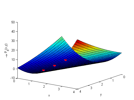
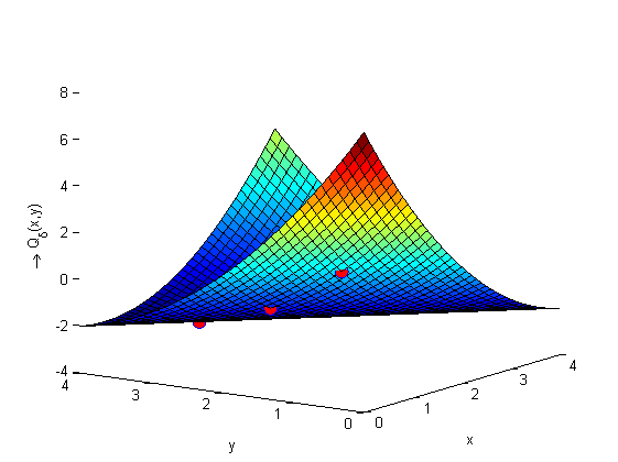
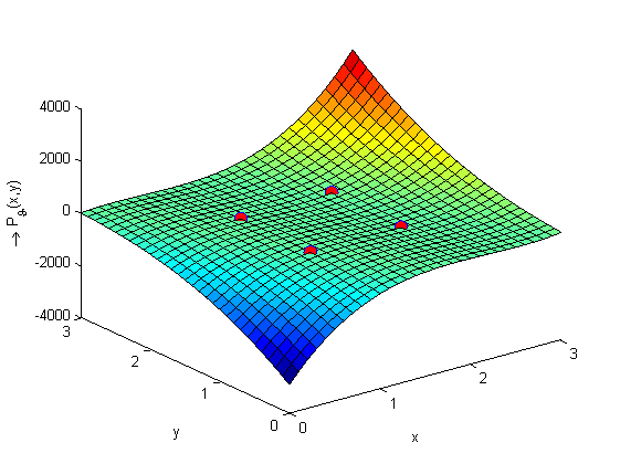
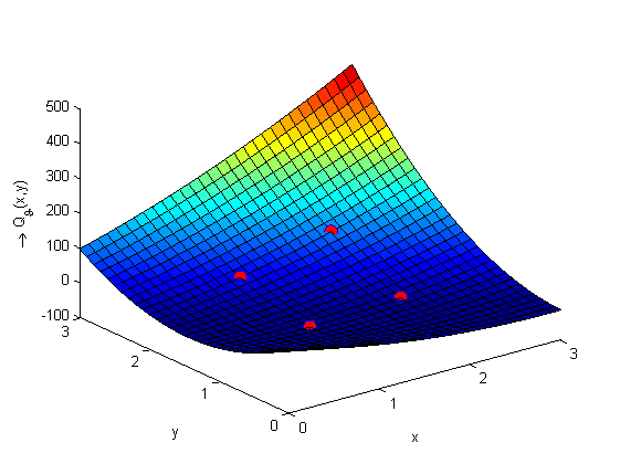
The surface diagrams in Figure 1 are demonstrating that the polynomials (3.1), (3.2), (3.3), and (3.4) satisfy all of the the data points of the matrices $\Theta$ and $\Psi$.

(a) $\wp_{\Theta}\in{{}_{1}^{3}\Pi_{1,3}^{2}}$

(b) ${\mathrm{p}}_{\Theta}\in{{}_{1}^{1}\Pi_{1,3}^{2}}$

(c) $\wp_{\Psi}\in{{}_{2}^{1}\Pi_{2,2}^{2}}$

(d) ${\mathrm{p}}_{\Psi}\in{{}_{1}^{2}\Pi_{2,2}^{2}}$

Figure 1. Surface diagrams of the interpolating polynomials (3.1), (3.2), (3.3) and (3.4) in the associated subspaces, showing the data points of the given matrices $\Theta$ and $\Psi$.

Example 3.2.

Let $\zeta\in\mathbb{R}^{2\times 2}$ is given as $\zeta=\begin{pmatrix}-1&2\\ 3&-4\end{pmatrix}$ and $I_{2}$ be the identity matrix of order 2. Then, $\zeta^{2}=\begin{pmatrix}7&-10\\ -15&22\end{pmatrix}$, and there exists unique $\wp_{\zeta},\wp_{\zeta^{2}},\wp_{I_{2}}\in{{}_{2}^{1}\Pi_{2,2}^{2}}$, such that

$$\wp_{\zeta}(x,y)=-(2x+y)^{3}+11(2x+y)^{2}-37(2x+y)+38,$$

$$\wp_{\zeta^{2}}(x,y)=5(2x+y)^{3}-54(2x+y)^{2}+176(2x+y)-170,$$

and $$\wp_{I_{2}}(x,y)=\frac{1}{2}(2x+y)^{2}-\frac{9}{2}(2x+y)+10.$$

This implies, $\wp_{\zeta^{2}}(x,y)-tr(\zeta).\wp_{\zeta}(x,y)+det(\zeta).\wp_{I_{2}}(x,y)=0$, where $tr(\zeta)=-5$ and $det(\zeta)=-2$. Hence, the associated polynomials satisfy the result of Cayley-Hamilton theorem in ${{}_{2}^{1}\Pi_{2,2}^{2}}$ for the given square matrix $\zeta$ in $\mathbb{R}^{2\times 2}$.

Example 3.3.

Let us consider the map ${\mathcal{T}}:\mathbb{R}^{2\times 2}\rightarrow\;_{2}^{1}\Pi_{2,2}^{2}$ defined by (2.13) and given as

(3.5) $${\mathcal{T}}{\left[\begin{pmatrix}a&b\\ c&d\end{pmatrix}\right]}= \frac{(-a+3b-3c+d)}{6}(2x+y)^{3}++\frac{(5a-14b+13c-4d)}{2}(2x+y)^{2}$$

$$+\frac{(-74a+189b-162c+47d)}{6}(2x+y)+(20a-45b+36c-10d).$$

Therefore, for every $A,B\in\mathbb{R}^{2\times 2}$ and some non-zero real scalar $\alpha$, we get

$${\mathcal{T}}{(\alpha A+B)}=\alpha{\mathcal{T}}(A)+{\mathcal{T}}(B),$$

i.e., the map (3.5) is linear.

Since $\mathfrak{B}_{1}=\left\{\begin{pmatrix}1&0\\ 0&0\end{pmatrix},\begin{pmatrix}0&1\\ 0&0\end{pmatrix},\begin{pmatrix}0&0\\ 1&0\end{pmatrix},\begin{pmatrix}0&0\\ 0&1\end{pmatrix}\right\}$ and $\mathfrak{B}_{2}={\{1,(2x+y),(2x+y)^{2},(2x+y)^{3}\}}$ be the standard bases of $\mathbb{R}^{2\times 2}$ and ${}_{2}^{1}\Pi_{2,2}^{2}$ respectively. Therefore,

$$\mathcal{T}{\left[\begin{pmatrix}1&0\\ 0&0\end{pmatrix}\right]}=20-\frac{37}{3}{(2x+y)}+\frac{5}{2}{(2x+y)^{2}}-\frac{1}{6}{(2x+y)^{3}},$$

$$\mathcal{T}{\left[\begin{pmatrix}0&1\\ 0&0\end{pmatrix}\right]}=-45+\frac{63}{2}{(2x+y)}-7{(2x+y)^{2}}+\frac{1}{2}{(2x+y)^{3}},$$

$$\mathcal{T}{\left[\begin{pmatrix}0&0\\ 1&0\end{pmatrix}\right]}=36-27{(2x+y)}+\frac{13}{2}{(2x+y)^{2}}-\frac{1}{2}{(2x+y)^{3}},$$

and $$\mathcal{T}{\left[\begin{pmatrix}0&0\\ 0&1\end{pmatrix}\right]}=-10+\frac{47}{6}{(2x+y)}-2{(2x+y)^{2}}+\frac{1}{6}{(2x+y)^{3}}.$$

Hence, the associated co-ordinate matrix with respect to the bases $\mathfrak{B}_{1}$ and $\mathfrak{B}_{2}$ is

(3.6) $$[{\mathcal{T}}]_{\mathfrak{B}_{1}}^{\mathfrak{B}_{2}}=\begin{pmatrix}20&-45&36&-10\\ -\frac{37}{3}&\frac{63}{2}&-27&\frac{47}{6}\\ \frac{5}{2}&-7&\frac{13}{2}&-2\\ -\frac{1}{6}&\frac{1}{2}&-\frac{1}{2}&\frac{1}{6}\end{pmatrix}.$$

Clearly, $det{\left([{\mathcal{T}}]_{\mathfrak{B}_{1}}^{\mathfrak{B}_{2}}\right)}\neq 0$, i.e., $\ker{\mathcal{T}}\neq 0$. Hence, the polynomial map (3.5) is invertible and thus consequently an isomorphism. Again, the map ${\mathcal{S}}:\;_{2}^{1}\Pi_{2,2}^{2}\rightarrow\mathbb{R}^{2\times 2}$ can be written as

(3.7) $${\mathcal{S}}{\left(a+bX+cX^{2}+dX^{3}\right)}=\begin{pmatrix}a+3b+9c+27d&a+4b+16c+64d\\ a+5b+25c+125d&a+6b+36c+216d\end{pmatrix},$$

where $X=2x+y$. The associated co-ordinate matrix with respect to the bases $\mathfrak{B}_{2}$ and $\mathfrak{B}_{1}$ is

(3.8) $$[{\mathcal{S}}]_{\mathfrak{B}_{2}}^{\mathfrak{B}_{1}}=\begin{pmatrix}1&3&9&27\\ 1&4&16&64\\ 1&5&25&125\\ 1&6&36&216\end{pmatrix},$$

such that $det{\left([{\mathcal{S}}]_{\mathfrak{B}_{2}}^{\mathfrak{B}_{1}}\right)}\neq 0$. Using (3.6) and (3.8), we get

$$[{\mathcal{T}}]_{\mathfrak{B}_{1}}^{\mathfrak{B}_{2}}.[{\mathcal{S}}]_{\mathfrak{B}_{2}}^{\mathfrak{B}_{1}}=\begin{pmatrix}1&0&0&0\\ 0&1&0&0\\ 0&0&1&0\\ 0&0&0&1\end{pmatrix}=[{\mathcal{S}}]_{\mathfrak{B}_{2}}^{\mathfrak{B}_{1}}.[{\mathcal{T}}]_{\mathfrak{B}_{1}}^{\mathfrak{B}_{2}}.$$

This shows that the maps given by (3.7) and (3.5) are inverse maps of each other.

Note 3.4.

The result of Corollary 2.5 and Theorem 2.7 are proved using a numerical approach of bivariate polynomial interpolation. The Example 3.2 and 3.3 validate them using some of the well-defined approaches and results of linear algebra. They also indicate a possible application of the results in the linear algebra community.

Example 3.5.

Let $\Omega=\left(f(i,j)\right)\in\mathbb{R}^{2\times 2}$ be a matrix generated by the real-valued function $f(x,y)=3{x^{2}}+2{y^{3}}-{x^{2}}y+2x{y^{2}}+x-y+10$. Then,

(3.9) $${\mathrm{p}}_{\Omega}(x,y) ={~{}}\frac{1}{2}{(x+2y)^{3}}-6(x+2y)^{2}+\frac{65}{2}{(x+2y)}-41,$$

(3.10) $$P_{\Omega}(x,y) ={~{}}3xy+6x+15y-8.$$

Therefore, the absolute error of the interpolating polynomial ${\mathrm{p}}_{\Omega}\in{{}_{1}^{2}\Pi_{2,2}^{2}}$ can be given as

(3.11) $$E_{{\mathrm{p}}_{\Omega}\in{{}_{1}^{2}\Pi_{2,2}^{2}}}=\lvert f(x,y)-{\mathrm{p}}_{\Omega}(x,y)\rvert,\quad(x,y)\in[1,2]\times[1,2],$$

and the absolute error of the interpolating polynomial $P_{\Omega}\in\Pi_{2}^{1}\times\Pi_{2}^{1}$ can be given as

(3.12) $$E_{P_{\Omega}\in\Pi_{2}^{1}\times\Pi_{2}^{1}}=\lvert f(x,y)-{P}_{\Omega}(x,y)\rvert,\quad(x,y)\in[1,2]\times[1,2].$$

The computation of the difference of errors, given by (3.11) and (3.11), of the interpolating polynomials (3.9) and (3.10) in ${{}_{1}^{2}\Pi_{2,2}^{2}}$ and $\Pi_{2}^{1}\times\Pi_{2}^{1}$ respectively, at equally spaced interpolating bivariate mesh-grid points with step-size 0.1 in $(x,y)\in[1,2]\times[1,2]$, is shown in Table 3.

Table 3. Absolute error difference of interpolating polynomials in the interpolation spaces ${{}_{1}^{2}\Pi_{2,2}^{2}}$ and $\Pi_{2}^{1}\times\Pi_{2}^{1}$, corresponds to the respective BVPIPM with respect to 2 by 2 grid points, for the matrix $\Omega=\left(f(i,j)\right)\in\mathbb{R}^{2\times 2}$ which is generated by a given function (smooth) $f:\mathbb{R}^{2}\rightarrow{\mathbb{R}}$.

Calculation of the error difference, $E_{{\mathrm{p}_{\Omega}}\in{{}_{1}^{2}\Pi_{2,2}^{2}}}-E_{P_{\Omega}\in\Pi_{2}^{1}\times\Pi_{2}^{1}}$ = $\lvert f(x,y)-{\mathrm{p}}_{\Omega}(x,y)\rvert-\lvert f(x,y)-P_{\Omega}(x,y)\rvert$,
at the equally spaced mesh-grid points in $(x,y)\in[1,2]\times[1,2]$ with step size 0.1, up to 4 decimal places.
$\downarrow\textbf{y}$ $\rightarrow\textbf{x}$	1	1.1	1.2	1.3	1.4	1.5	1.6	1.7	1.8	1.9	2
1	0	0.0855	0.1439	0.1785	0.1920	0.1875	0.1679	0.1365	0.0959	0.0495	0
1.1	0.1439	0.1485	0.1320	0.0975	0.0479	-0.0135	-0.0839	-0.1605	-0.2400	-0.3195	-0.3959
1.2	0.1920	0.1275	0.0479	-0.0435	-0.1440	-0.2505	-0.3599	-0.4695	-0.5759	-0.6765	-0.7680
1.3	0.1679	0.0465	-0.0840	-0.2205	-0.3599	-0.4995	-0.6359	-0.7665	-0.8880	-0.9975	-1.0919
1.4	0.0959	-0.0705	-0.2399	-0.4095	-0.5760	-0.7365	-0.8880	-1.0275	-1.1519	-1.2585	-1.3440
1.5	0	-0.1995	-0.3959	-0.5865	-0.7680	-0.9375	-1.0919	-1.2285	-1.3440	-1.4355	-1.5000
1.6	-0.0959	-0.3165	-0.5280	-0.7275	-0.9119	-1.0785	-1.2239	-1.3455	-1.4399	-1.5045	-1.5360
1.7	-0.1680	-0.3975	-0.6119	-0.8085	-0.9840	-1.1355	-1.2600	-1.3545	-1.4160	-1.4415	-1.4280
1.8	-0.1919	-0.4185	-0.6240	-0.8055	-0.9600	-1.0845	-1.1760	-1.2315	-1.2480	-1.2225	-1.1519
1.9	-0.1440	-0.3555	-0.5399	-0.6945	-0.8160	-0.9015	-0.9480	-0.9525	-0.9119	-0.8235	-0.6840
2	0	0.0045	0.0159	0.0315	0.0480	0.0625	0.0719	0.0735	0.0640	0.0405	0

From Table 3, it can be observed that the absolute error of the interpolating polynomial ${\mathrm{p}_{\Omega}}(x,y)$ in ${{}_{1}^{2}\Pi_{2,2}^{2}}$ is moreover less in comparison of the interpolating polynomial $P_{\Omega}(x,y)$ in $\Pi_{2}^{1}\times\Pi_{2}^{1}$, at most of the interpolating points in $(x,y)\in[1,2]\times[1,2]$.

4. Concluding remarks

In this article, the existence of a specific class of $mn$-dimensional interpolation spaces, in a space of BVPS of the form ${}_{\alpha}^{\beta}\Pi_{m,n}^{2}$, has been established for a proposed BVPIPM (* ‣ 1.1) with respect to a set of special nodes $\Xi$. Also, some exclusive isomorphisms from $\mathbb{R}^{m\times n}$ to ${}_{n}^{1}\Pi_{mn-1}^{2}$ and ${}_{1}^{m}\Pi_{mn-1}^{2}$ are formulated, which satisfy an additional condition of the BVPIPM (* ‣ 1.1) with respect to $\Xi$. For this, a different approach of bivariate polynomial interpolation is applied. The BVPIPM (* ‣ 1.1) is reduced to a univariate polynomial interpolation problem, using a transformation $\phi:\Xi\rightarrow\mathbb{R}$,$(i,j)\rightarrow{\alpha i+\beta j}$ and $z=\alpha x+\beta y$, where $\alpha>0$ and $\beta>0$ such that $\phi$ is bijective. In these cases, it can be said that the solution of the BVPIPM (* ‣ 1.1) is equivalent to the univariate polynomial interpolation when all of the points are projected to a line orthogonal to $\alpha x+\beta y=0$, which are chosen such that all projections are different.

To be sure, the polynomial space ${}_{\alpha}^{\beta}\Pi_{m,n}^{2}$ is correct for any $m$ by $n$ rectangular grid for uncountably many choices of $\alpha$ and $\beta$ and fulfills the necessary condition of correctness. In spite of this, this polynomial space has an unfortunate bias: all its elements are constant in the direction $(-\beta,\alpha)$, which is somehow quite unnatural for interpolation on a rectangular mesh. It can be said that the established interpolation spaces do not perfectly fulfill the respective sufficient condition for ‘good’ interpolation. However, for some of the BVPIPM’s with respect to $m$ by $n$ rectangular grid points, the associated interpolating polynomials in some of these interpolation spaces possibly reduce the absolute error as compared to the bivariate interpolating polynomials in the standard tensor product space of two univariate polynomial subspaces (see Example 3.5). Overall, the outcomes of the article are adding some additional tools to linear algebra and numerical linear algebra community.

The authors are working to submit some potential applications of the BVPIPM (* ‣ 1.1) in mathematics and some other branches of science and engineering. We take these as our future objectives and the possible suggestions or work in this direction would be highly complementary.

5. Acknowledgement

The first author is thankful to University Grant Commission (UGC), India, for the award of a research fellowship under NET/JRF scheme with reference number 1086/(OBC)(CSIR-UGC NET DEC. 2016).

Appendix A Non-poisedness of the BVPIPM

In this section, we are providing some illustrations to demonstrate that the BVPIPM (* ‣ 1.1) with respect to $\Xi$ cannot be always poised in ${k+2}\choose{k}$-dimensional subspace $\Pi_{k}^{2}$, for a given $\alpha_{ij}\in\mathbb{R}^{m\times n}$, even if $\dim\Pi_{k}^{2}=mn$.

Exercise A.1.

Let $({\alpha_{ij}})\in\mathbb{R}^{3\times 1}$ be a given matrix. Then, for the known three data points $((1,1),a_{11})$, $((2,1),a_{21})$, and $((3,1),a_{31})$, the respective BVPIPM (* ‣ 1.1) can be written as

(A.1) $$\wp(i,j)=\alpha_{ij}\textrm{ for all }i=1,2,3,\;j=1.$$

Since $\dim\Pi_{1}^{2}=3$, the known set of data points may define an interpolating polynomial $\wp\in\Pi_{1}^{2}$. Let us assume that

(A.2) $$\wp(x,y)=ax+by+c,$$

where $a,b$ and $c$ are real constants. If the polynomial (A.2) satisfies the BVPIPM (A.1), the coefficients $a,b$ and $c$ must satisfy the system of equations

(A.3) $$a+b+c=\alpha_{11},2a+b+c=\alpha_{21},\textrm{ and }3a+b+c=\alpha_{31}.$$

The system of equations (A.3) is equivalent to

(A.4) $${\begin{pmatrix}1&1&1\\ 1&0&0\\ 0&0&0\end{pmatrix}}{\begin{pmatrix}a\\ b\\ c\end{pmatrix}}={\begin{pmatrix}\alpha_{11}\\ \alpha_{21}-\alpha_{11}\\ \alpha_{31}-2\alpha_{21}+\alpha_{11}\end{pmatrix}},$$

i.e., the determinant of the associated sample matrix (equivalently coefficient matrix) is zero. Hence, the BVPIPM (A.1) with respect to the interpolation points $(1,1)$, $(2,1)$, and $(3,1)$ cannot be poised in $\Pi_{1}^{2}$ for any given matrix in $\mathbb{R}^{3\times 1}$. Similarly, the BVPIPM (A.1) with respect to the interpolation points $(1,1)$, $(1,2)$, and $(1,3)$ cannot be poised in $\Pi_{1}^{2}$ for any given matrix in $\mathbb{R}^{1\times 3}$.

Exercise A.2.

Let $(\alpha_{ij})\in\mathbb{R}^{3\times 2}$ be a given matrix. Then, for the known six data points $((1,1),b_{11})$, $((1,2),b_{12})$, $((2,1),b_{21})$, $((2,2),b_{22})$, $((3,1),b_{31})$, and $((3,2),b_{32})$, the respective BVPIPM (* ‣ 1.1) can be written as

(A.5) $$\wp(i,j)=\alpha_{ij}\textrm{ for all }i=1,2,3,\;\;j=1,2.$$

Since $\dim\Pi_{2}^{2}=6$, the known set of data points may define an interpolating polynomial $\wp\in\Pi_{2}^{2}$. Let us assume that

(A.6) $$\wp(x,y)=a_{1}x^{2}+a_{2}xy+a_{3}y^{2}+a_{4}x+a_{5}y+a_{6},$$

where $a_{k},k=1,2,\ldots,6$ are real constants. If the polynomial (A.6) satisfies the BVPIPM (A.5), then the coefficients must satisfy

(A.7) $$\alpha_{ij}=a_{1}i^{2}+a_{2}ij+a_{3}j^{2}+a_{4}i+a_{5}j+a_{6};\;\;i=1,2,3,\;\;j=1,2.$$

The system of equations (A.7) is equivalent to

(A.8) $${\begin{pmatrix}1&1&1&1&1&1\\ 0&1&3&0&1&0\\ 4&2&1&2&1&1\\ 0&1&0&0&0&0\\ 9&3&1&3&1&1\\ 0&0&0&0&0&0\end{pmatrix}}{\begin{pmatrix}a_{1}\\ a_{2}\\ a_{3}\\ a_{4}\\ a_{5}\\ a_{6}\end{pmatrix}}={\begin{pmatrix}\alpha_{11}\\ \alpha_{12}-\alpha_{11}\\ \alpha_{21}\\ \alpha_{22}-\alpha_{21}-\alpha_{12}+\alpha_{11}\\ \alpha_{31}\\ \alpha_{32}-2\alpha_{22}+\alpha_{12}-\alpha_{31}+2\alpha_{21}-\alpha_{11}\end{pmatrix}}.$$

Therefore, the determinant of the associated sample matrix is zero. Hence, the BVPIPM (A.5) with respect to the nodes $(1,1),(1,2),(2,1),(2,2),(3,1)$, and $(3,2)$ cannot be poised in $\Pi_{2}^{2}$ for any given matrix in $\mathbb{R}^{3\times 2}$. Similarly, the BVPIPM (A.5) with respect to the nodes $(1,1),(1,2),(1,3),(2,1),(2,2)$, and $(2,3)$ cannot be poised in $\Pi_{2}^{2}$ for any given matrix in $\mathbb{R}^{2\times 3}$.

In the similar manner, we have verified that for the subspace $\Pi_{3}^{2}$ ($\dim\Pi_{3}^{2}=10)$, the determinant of the associated sample matrix, corresponding to the BVPIPM (* ‣ 1.1) with respect to $\Xi$ for any given matrix of the all possible orders $1\times 10$, $2\times 5$, $5\times 2$ and $10\times 1$, is zero.

Remark A.3.

For $\Pi_{k}^{2}$, such that $mn=\dim\Pi_{k}^{2}$, the construction of respective sample matrix of the order $\frac{(k+1)(k+2)}{2}\times\frac{(k+1)(k+2)}{2}$, corresponding to the BVPIPM (* ‣ 1.1) with respect to $\Xi$ for any given $(\alpha_{ij})\in\mathbb{R}^{m\times n}$, is analytically intractable for large $k$. Using a suitable computer program, it is verified that for any given matrix $(\alpha_{ij})\in\mathbb{R}^{m\times n}$, for which $mn=\dim\Pi_{k}^{2}$, the associated sample matrix of the BVPIPM (* ‣ 1.1) with respect to $\Xi$ is singular, upto $k\leq 30$. We conjecture that it is true for all $k\in\mathbb{N}$.

References

- [1] Fausto Saleri Alfio Quarteroni, Riccardo Sacco, Numerical mathematics, Texts in Applied Mathematics, Springer, Berlin, Heidelberg, 2007.
- [2] Martin Gander Anne Bourlioux, Modern methods in scientific computing and applications, 75, Springer Netherlands, 2002.
- [3] K. Atkinson, Elementary numerical analysis, Wiley, New York, 1985.
- [4] Sheldon Jay Axler, Linear algebra done right, third ed., Undergraduate Texts in Mathematics, Springer International Publishing, 2015.
- [5] Dario Bini and Victor Y. Pan, Polynomial and matrix computations (vol. 1): Fundamental algorithms, Birkhauser Verlag, Basel, Switzerland, Switzerland, 1994.
- [6] Jonathan C Carr, W Richard Fright, and Richard K Beatson, Surface interpolation with radial basis functions for medical imaging, IEEE transactions on medical imaging 16 (1997), no. 1, 96–107.
- [7] Z.Y. Chen, Computer aided design in control systems 1988: Selected papers from the 4th ifac symposium, beijing, prc, 23-25 august 1988, IFAC Symposia Series, Elsevier Science, 2017.
- [8] Mariano Gasca and Thomas Sauer, On the history of multivariate polynomial interpolation, Journal of Computational and Applied Mathematics 122 (2000), no. 1, 23 – 35, Numerical Analysis in the 20th Century Vol. II: Interpolation and Extrapolation.
- [9] by same author, Polynomial Interpolation in Several Variables, Advances in Computational Mathematics 12 (2000), 377–410.
- [10] Paul Kergin, A natural interpolation of ck functions, Journal of Approximation Theory 29 (1980), no. 4, 278–293.
- [11] Allen Klinger, The Vandermonde Matrix, The American Mathematical Monthly 74 (1967), no. 5, 571–574.
- [12] U. Langer and P. Paule, Numerical and symbolic scientific computing: Progress and prospects, Texts & Monographs in Symbolic Computation, Springer Vienna, 2011.
- [13] P.M. Larsen and N.E. Hansen, Computer aided design in control and engineering systems: Advanced tools for modern technology, IFAC proceedings series, Elsevier Science, 2014.
- [14] S. Levy, L. Velho, A.C. Frery, and J. Gomes, Image processing for computer graphics and vision, Texts in Computer Science, Springer London, 2009.
- [15] H Michael Möller and Thomas Sauer, H-bases for polynomial interpolation and system solving, Advances in Computational Mathematics 12 (2000), no. 4, 335–362.
- [16] Seimatsu Narumi, Some formulas in the theory of interpolation of many independent variables, Tohoku Mathematical Journal, First Series 18 (1920), 309–321.
- [17] Thomas Sauer, Polynomial Interpolation in Several Variables: Lattices, Differences, and Ideals, Studies in Computational Mathematics 12 (2006), 191–230.
- [18] Thomas Sauer and Yuan Xu, On multivariate lagrange interpolation, Mathematics of Computation 64 (1995), no. 211, 1147–1170.
- [19] E. Sciubba, G. Manfrida, and U. Desideri, Ecos 2012 the 25th international conference on efficiency, cost, optimization and simulation of energy conversion systems and processes (perugia, june 26th-june 29th, 2012), Proceedings e report, Firenze University Press, 2012.
- [20] M. Sonka, V. Hlavac, and R. Boyle, Image processing, analysis, and machine vision, Cengage Learning, 2014.