Simple Impedance Response Formulas for the Dispersive Interaction Rates in the Effective Hamiltonians of Low Anharmonicity Superconducting Qubits

Abstract

For superconducting quantum processors consisting of low anharmonicity qubits such as transmons we give a complete microwave description of the system in the qubit subspace. We assume that the qubits are dispersively coupled to a distributed microwave structure such that the detunings of the qubits from the internal modes of the microwave structure are stronger than their couplings. We define “qubit ports” across the terminals of the Josephson junctions and “drive ports” where transmission lines carrying drive signals reach the chip and we obtain the multiport impedance response of the linear passive part of the system between the ports. We then relate interaction parameters in between qubits and between the qubits and the environment to the entries of this multiport impedance function: in particular we show that the exchange coupling rate $J$ between qubits is related in a simple way to the off-diagonal entry connecting the qubit ports. Similarly we relate couplings of the qubits to voltage drives and lossy environment to the entries connecting the qubits and the drive ports. Our treatment takes into account all the modes (possibly infinite) that might be present in the distributed electromagnetic structure and provides an efficient method for the modeling and analysis of the circuits.

I Introduction

Superconducting circuits are a promising platform for the realization of quantum computers. Operated at microwave frequencies they include Josephson junctions for the non-linearity needed to obtain qubit modes without introducing significant loss. Coherence times of the superconducting qubits have been improved by several orders of magnitude in the last two decades and the Transmon qubit Koch-Transmon ; Zombie-paper-Gambetta (and its several variations Xmon ; Dicarlo ) has now become the superconducting qubit of choice in many groups around the world due to its simplicity of design and its superior coherence. Fidelities of the single qubit gates are now routinely below Martinis-Nature ; Sarah-Single-Qubit and those of the two-qubit gates are at the fault-tolerance threshold levels required by the surface code Martinis-Nature ; Sarah-CR ; Maika-Parity . The challenge now is to scale the circuits up while maintaining and improving further the qubit coherence times and gate fidelities Nick . Many important engineering problems however arise in the design of larger multi-qubit devices such as signal crosstalk and qubit-qubit crosstalk which show the need for better models/tools to understand and improve the operation of the superconducting quantum processors.

Several methods have been used to model and study the physics of superconducting qubit circuits. The Jaynes-Cummings model Jaynes-Cummings originally introduced in quantum optics has routinely been applied to the study of the so-called circuit-QED architecture Blais-xQED ; Wallraff in which superconducting qubits are coupled to readout resonators for their control and readout and two-qubit gate operations are mediated by the bus resonators. Readout and bus resonators are typically designed to be detuned away from the qubits to operate in the so-called dispersive regime. In that regime one can eliminate the resonators up to desired order in the bare qubit-resonator couplings and get an effective description of the system in the qubit subspace. However calculation of the dispersive quantities such as the exchange coupling or Purcell decay rates Controlling Spontaneous Emission - Houck of the qubits with the single mode Jaynes-Cummings model showed significant discrepancy with the experimental measurements and attempts to include higher harmonics of the resonators with multi-mode extensions of the Jaynes-Cummings model failed due to divergence issues Bourassa-Multi-Mode-circuit-QED . Gely-Adrian-Solano showed the convergence of the Lamb shift in the specific case of a Josephson junction atom coupled to a multimode resonator in the Rabi model. More recently Adrian-Long studied the convergence of the bare couplings between the superconducting qubits and multimode resonators in various general coupling configurations.

Combination of lumped element circuit quantization methods Devoret-Les-Houches ; BKD ; Burkard with classical circuit synthesis techniques Foster ; Brune ; Newcomb resulted in “blackbox quantization” methods BBQ-Yale ; Brune-Quantization ; Solgun which allowed extraction of the parameters in the quantum Hamiltonian models of the superconducting circuits from the electromagnetic finite-element simulations. The simulations correspond to the linear passive part of the circuits which is usually a distributed microwave structure as seen looking into the ports defined across the Josephson junctions. Although such an approach allows an accurate treatment of very general structures consisting possibly of multiple microwave modes simulation of large multi-qubit devices might quickly become computationally demanding.

Following a similar approach we show here that for superconducting processors consisting of low anharmocity qubits like transmons the dispersive interaction parameters such as exchange coupling and Purcell decay rates of the qubits and their coupling to the voltage drives are related in a simple way to the microwave impedance response functions as seen at the “qubit ports” and “drive ports”. This reduces a large portion of the design of multi-qubit superconducting devices into a classical microwave engineering problem (up to the assumptions and approximations we are making here) and allows one to avoid any numerical multi-mode block-diagonalization or fitting of electromagnetic finite-element simulations over a range of frequencies which are both expensive if not prohibitive computational procedures.

We propose the following effective Hamiltonian to desribe a multi-qubit superconducting device consisting of low anharmonicity qubits coupled to each other and to the external world through a linear passive distributed microwave structure:

$$\hat{\mathcal{H}}/\hbar = \stackrel{{\scriptstyle[}}{{i}}=1]{N}{\sum}\omega_{i}\hat{b}_{i}^{\dagger}\hat{b}_{i}+\frac{\delta_{i}}{2}\hat{b}_{i}^{\dagger}\hat{b}_{i}(\hat{b}_{i}^{\dagger}\hat{b}_{i}-1)+\underset{i,j}{\sum}J_{ij}(\hat{b}_{i}\hat{b}_{j}^{\dagger}+\hat{b}_{i}^{\dagger}\hat{b}_{j})+\stackrel{{\scriptstyle[}}{{i}}=1]{N}{\sum}\stackrel{{\scriptstyle[}}{{d}}=1]{N_{D}}{\sum}\varepsilon_{id}(\hat{b}_{i}-\hat{b}_{i}^{\dagger})V_{d}$$ (1)

$$+ \underset{i,k}{\sum}\chi_{ik}\hat{b}_{i}^{\dagger}\hat{b}_{i}\hat{a}_{k}^{\dagger}\hat{a}_{k}+\stackrel{{\scriptstyle[}}{{k}}=1]{M}{\sum}\omega_{R_{k}}\hat{a}_{k}^{\dagger}\hat{a}_{k}+\frac{\chi_{kk}^{(R)}}{2}\hat{a}_{k}^{\dagger}\hat{a}_{k}(\hat{a}_{k}^{\dagger}\hat{a}_{k}-1)+\underset{k,k^{\prime}}{\sum}J_{kk^{\prime}}^{\left(R\right)}(\hat{a}_{k}\hat{a}_{k^{\prime}}^{\dagger}+\hat{a}_{k}^{\dagger}\hat{a}_{k^{\prime}})$$

where we have $N$ qubit modes and $M$ resonator modes represented as Duffing oscillators in the harmonic oscillator basis and $N_{D}$ voltage drives. In the first line we have terms corresponding to the qubit subspace: $\hat{b}_{i}^{(\dagger)}$ is the annihilation(creation) operator of the qubit mode $i$ of frequency $\omega_{i}$ and anharmonicity $\delta_{i}$. In the second line we have the resonator terms: $\hat{a}_{k}^{(\dagger)}$ is the annihilation(creation) operator of the resonator mode $k$ with frequency $\omega_{R_{k}}$ and anharmonicity (or self-Kerr) $\chi_{kk}^{(R)}$ (We will be using the terms “resonator” and “internal mode” interchangibly below to refer to the microwave modes of the distributed linear passive structure the qubits are connected to). Such an approximate description in the harmonic basis is valid for qubits with low anharmonicity $\delta_{i}\ll\omega_{i}$ such as transmons. Qubit modes $i$ and $j$ are coupled to each other at exchange coupling rate $J_{ij}$ and the only remaining interaction between the qubit and resonator modes are the dispersive energy shifts $\chi_{ik}$’s.

We show that the exchange coupling rate $J_{ij}$ between qubit modes $i$ and $j$ in such an effective description is a simple function of the impedance response defined between the “qubit ports”

$$J_{ij}=-\frac{1}{4}\sqrt{\frac{\omega_{i}\omega_{j}}{L_{i}L_{j}}}\mathrm{Im}\left[\frac{Z_{ij}\left(\omega_{i}\right)}{\omega_{i}}+\frac{Z_{ij}\left(\omega_{j}\right)}{\omega_{j}}\right]$$ (2)

where $\omega_{i}$ is the frequency of the qubit $i$ given by $\omega_{i}=\omega_{J_{i}}-\frac{E_{C}^{(i)}/\hbar}{1-E_{C}^{(i)}/(\hbar\omega_{J_{i}})}$ with $\omega_{J_{i}}=1/\sqrt{L_{J_{i}}C_{i}}$ and $E_{C}^{(i)}=\frac{e^{2}}{2C_{i}}$ being the charging energy of the qubit $i$ of total shunt capacitance $C_{i}$. $L_{i}$ and $L_{j}$ are the “qubit inductances” corresponding to the qubits $i$ and $j$, respectively; related to the bare junction inductances $L_{J_{i}}$’s by $L_{i}=L_{J_{i}}/(1-\frac{2E_{C}^{(i)}}{\hbar\omega_{i}}$) such that $\omega_{i}=1/\sqrt{L_{i}C_{i}}$. $Z_{ij}\left(\omega\right)$ is the $\left(i,j\right)$-entry of the multiport impedance matrix $\mathbf{Z}(\omega)$ connecting $i^{th}$ qubit’s port to the $j^{th}$ qubit’s port. Qubit ports are defined between the terminals of the Josephson junctions; i.e. port voltages are voltages developed across and the port currents are the currents flowing through the Josephson junctions (See also Appendix (VIII.3) for how to define qubit ports as lumped ports in electromagnetic simulators). The multiport impedance matrix $\mathbf{Z}(\omega)$ is to be computed between the qubit ports with Josephson junctions removed. $\mathbf{Z}(\omega)$ then gives the response of the linear part of the circuit seen by looking into the qubit ports; in particular $Z_{ij}(\omega)$ is the voltage developed across $i^{th}$ qubit’s port while a current of unit magnitude and frequency $\omega$ is driving $j^{th}$ qubit’s port while all other qubit ports left open. We note here that the formula in Eq. (2) holds in the case of a distributed microwave structure consisting of multiple internal modes(possibly infinite) coupling the qubits.

$V_{d}$ in Eq. (1) is the voltage source driving the $d$-th drive line for $1\leq d\leq N_{D}$ (Assuming there are a total of $N_{D}$ lines driving the system as shown in Fig. LABEL:fig:Cauer-circuit-with-drives) and $\varepsilon_{id}$ is the matrix entry giving the coupling of the qubit $i$ to the voltage source $V_{d}$. In Section (VIII.2) we show that (under the assumption that no off-chip crosstalk is happening between the drive lines)

$$\varepsilon_{id}=\sqrt{\frac{\omega_{i}}{2\hbar L_{i}}}\mathrm{Im}\left[Z_{i,p(d)}(\omega_{i})\right]\frac{e^{i\theta_{d}}C_{p(d)}}{\sqrt{1+\omega_{d}^{2}Z_{0}^{2}C_{p(d)}^{2}}}$$ (3)

where $\theta_{d}=\frac{\pi}{2}-\arctan(\omega_{d}Z_{0}C_{p(d)})$ and $Z_{i,p(d)}(\omega_{i})$ is the entry of the multiport impedance matrix connecting the drive port(with port index $p(d)$) corresponding to the voltage source $V_{d}$ (for the definition of drive ports see Section (III.1) and Appendix (VIII.3)) to the qubit port $i$ evaluated at the frequency $\omega_{i}$ of qubit $i$; $\omega_{d}$ is the frequency of the voltage source $V_{d}$(assuming a single tone sinusoidal signal), $Z_{0}$ is the characteristic impedance of the drive lines which is typically $Z_{0}=50\Omega$ and $C_{p(d)}$ is the shunting capacitance of the drive port corresponding to the voltage source $V_{d}$. Since the drive ports are defined where the drive lines reach the chip the factor $\mathrm{Im}\left[Z_{i,p(d)}(\omega_{i})\right]$ in Eq. (3) gives the classical crosstalk happening at the trasition region where the lines land onto the chip or on the chip. We also calculate below the following in units of $dB$ as a measure of the classical crosstalk assuming similar values for qubit parameters in Eq. (3)

$$X_{ij}=20\mathrm{log}_{10}\left(\frac{\mathrm{Im}[Z_{i,d(j)}(\omega_{i})]}{\mathrm{Im}[Z_{j,d(j)}(\omega_{j})]}\right)$$ (4)

where $d(j)$ is the port index of the drive of the qubit $j$ . $X_{ij}$ is the voltage crosstalk in $dB$ seen by qubit $i$ while driving qubit $j$.

The resonance frequency $\omega_{R_{k}}$ of the resonator $k$ gets the dispersive shift $\chi_{ik}$ depending on the state of the qubit $i$. We calculate $\chi_{ik}$ in Section (V) similar to what has been done in BBQ-Yale by including the fourth order nonlinear terms in the junction potentials

$$\chi_{ik}=8\delta_{i}\left(\frac{g_{ik}\omega_{R_{k}}}{\omega_{R_{k}}^{2}-\omega_{i}^{2}}\right)^{2}$$ (5)

where $\delta_{i}$ is the anharmonicity of the qubit mode $i$ given in Eq. (57) as $\delta_{i}=-E_{C}^{(i)}(\omega_{J_{i}}/\omega_{i})^{2}$ and $g_{ik}$ is the bare coupling rate between the qubit mode $i$ and the resonator mode $k$ given in Eq. (11) below.

We assume that the losses in the system are small; in particular we neglect any internal loss. Hence $\mathrm{Im}[\mathbf{Z}(\omega)]$ describes the lossless part of the system to a very good approximation. In Section (IV) we describe how to include the effect of external losses due to the coupling to drive lines by computing Purcell rates for the qubit modes. We show that the Purcell loss rate $\frac{1}{T_{1}^{i,d}}$ of qubit $i$ due to the drive line $d$

$$\frac{1}{T_{1}^{i,d}}=\frac{2}{L_{i}}\mathrm{Im}\left[Z_{i,p(d)}\left(\omega_{i}\right)\right]^{2}\frac{\omega_{i}^{2}Z_{0}C_{p(d)}^{2}}{1+\omega_{i}^{2}Z_{0}^{2}C_{p(d)}^{2}}$$ (6)

We note here that all the dispersive rates of qubit-qubit interactions and of interactions of qubits with the external electronics are functionals of the the multiport impedance function $\mathbf{Z}(\omega)$ and bare junction inductances $L_{J_{i}}$’s since the shunting capacitances $C_{i}$’s of the qubit ports are related to the residue $\mathbf{A}_{0}$ of $\mathbf{Z}(\omega)$ at DC as given in Eq. (61) (Same argument applies to the shunt capacitances $C_{p(d)}$’s of the drive ports) and the qubit frequencies $\omega_{i}$’s and anharmonicities $\delta_{i}$’s are functions of qubit shunt capacitances and bare junction inductances.

$J_{kk^{\prime}}^{\left(R\right)}$ in the second line in Eq. (1) are exchange coupling rates between resonator modes mediated by the qubits. We note here that terms of the form $\chi_{iikk^{\prime}}\hat{b}_{i}^{\dagger}\hat{b}_{i}\hat{a}_{k}^{\dagger}\hat{a}_{k^{\prime}}$ that are usually dropped by rotating wave approximation might be comparable to other terms in Eq. (1) if the frequencies $\omega_{R_{k}}$, $\omega_{R_{k^{\prime}}}$ of resonators $k$, $k^{\prime}$ are not detuned enough. In Eq. (1) we also neglected drive terms on the resonators.

II Derivation of the Formula for the Exchange Coupling Rates between the Qubits

Assuming we have $N$ Josephson junctions in the circuit we define the $N\times N$ multiport impedance matrix $\mathbf{Z}$ seen looking into qubit ports defined across the junction terminals ($\mathbf{Z}$ has to be evaluated without shunting the qubit ports by Josephson junctions). Neglecting all the losses we can write the following partial fraction expansion for the imaginary part of $\mathbf{Z}\left(\omega\right)$ as a function of the frequency variable $\omega$ Newcomb

$$\mathbf{Z}_{I}\left(\omega\right) = \mathrm{Im}\left[\mathbf{Z}\left(\omega\right)\right]$$ (7)

$$= -\frac{\mathbf{A}_{0}}{\omega}+\stackrel{{\scriptstyle[}}{{k}}=1]{M}{\sum}\frac{\mathbf{A}_{k}\omega}{\omega_{R_{k}}^{2}-\omega^{2}}+\mathbf{A}_{\infty}\omega$$

where $\omega_{R_{k}}$’s are the frequencies of the internal modes corresponding to readout and bus resonators and $\mathbf{A}_{k}$’s are rank-1 DDV real symmetric $N\times N$ matrices for $1\leq k\leq M$. Although we have truncated the part corresponding to internal modes to $M$ terms as we will see below the formula in Eq. (2) stays valid in the limit of an infinite number of modes $M\rightarrow\infty$ (more generally one can think of the multiport impedance expansion in Eq. (7) as being corresponding to any distributed electromagnetic structure seen by the junctions).

Starting with the expansion in Eq. (7) we can synthesize a lossless multiport lumped element circuit Newcomb as shown in Fig. (LABEL:fig:Cauer-circuit). We see $N$ qubit ports on the left in Fig. (LABEL:fig:Cauer-circuit) which are shunted by Josephson junctions. Using the method described in Burkard we can identify the degrees of freedom in this circuit and derive the following Hamiltonian (see Appendix (VIII.1))

$$\mathcal{H}=\frac{1}{2}\mathbf{Q}^{T}\mathbf{C}^{-1}\mathbf{Q}+\frac{1}{2}\mathbf{\Phi}^{T}\mathbf{M}_{0}\mathbf{\Phi}-\stackrel{{\scriptstyle[}}{{i}}=1]{N}{\sum}E_{J_{i}}\cos\left(\varphi_{J_{i}}\right)$$ (8)

where $\mathbf{\Phi}=\left(\Phi_{J_{1}},\ldots,\Phi_{J_{N}},\Phi_{R_{1}},\ldots,\Phi_{R_{M}}\right)^{T}$ being the flux coordinate vector. $\varphi_{J_{i}}$ is the phase of the junction $i$ related to the flux across it by the Josephson relation $\Phi_{J_{i}}=\frac{\mathrm{\Phi}_{0}}{2\pi}\varphi_{J_{i}}$, for $1\leq i\leq N$. $\Phi_{R_{k}}$ is the flux across the inductor of the internal mode $k,$ $1\leq k\leq M$. $E_{J_{i}}$ is the Josephson energy of junction $i$ related to its inductance $L_{J_{i}}$ by $E_{J_{i}}=\left(\frac{\mathrm{\Phi}_{0}}{2\pi}\right)^{2}\frac{1}{L_{J_{i}}}$. The capacitance matrix $\mathbf{C}$ is given by

$$\mathbf{C}=\left(\begin{array}[]{cc}\mathbf{C}_{0}&-\mathbf{C}_{0}\mathbf{R}^{T}\\ -\mathbf{R}\mathbf{C}_{0}&\mathbf{1}_{M\times M}+\mathbf{R}\mathbf{C}_{0}\mathbf{R}^{T}\end{array}\right)$$ (9)

where $\mathbf{C}_{0}$ is diagonal with entries $\left(C_{1},\ldots,C_{N}\right)$, $C_{i}$ being the total capacitance shunting the junction $i$. This is a valid physical assumption since it corresponds to having no direct electrostatic dipole-dipole interaction between junction terminals. Such an assumption will keep our discussion simple although the case of non-diagonal $\mathbf{C}_{0}$ will not change any of the results. In such a case one can treat the non-diagonal part of $\mathbf{C}_{0}$ at frequency $\epsilon$ like the other terms at finite frequencies $\omega_{R_{k}}$’s in the impedance expansion in Eq. (7) and apply the Scrieffer-Wolff transformation as described below in the limit of $\epsilon\rightarrow 0$ (A more rigorous algorithm in the case of non-diagonal $\mathbf{C}_{0}$ would be to remove as much diagonal part of $\mathbf{C}_{0}$ as possible while keeping the rest still positive semidefinite and apply the small $\epsilon$ frequency treatment we just described to an eigendecomposition of the non-diagonal part).

$\mathbf{R}$ is a $M\times N$ matrix generating the couplings between qubits and internal modes. $\mathbf{R}$ consists of row vectors $r_{k}=\left(r_{k1}\ldots r_{kN}\right)$ with $r_{k}^{T}r_{k}=\mathbf{A}_{k}$. $\mathbf{M}_{0}$ matrix is diagonal with entries $\left(1/L_{1},\ldots,1/L_{N},1/L_{R_{1}},\ldots,1/L_{R_{M}}\right)$ where $L_{R_{k}}=1/\omega_{R_{k}}^{2}$ for $1\leq k\leq M$. Here we replaced the Josephson junction $i$ with the qubit inductance $L_{i}$ such that $1/\sqrt{L_{i}C_{i}}=\omega_{i}$. An important point to note here is that the choice of $L_{i}$ over the bare junction inductance $L_{J_{i}}$ makes the two-body terms(that appear after expanding the nonlinear terms in the junction potentials and normal ordering) in Eq. (10) of BBQ-Yale vanish up to the order of interest here. This is crucial since these terms might contain significant residual couplings between qubit and internal modes. We refer the reader to Appendix (VIII.4) for details.

We do a capacitance rescaling Brito $\mathbf{\Phi}_{J}\rightarrow\mathbf{C}_{0}^{1/2}\mathbf{\Phi}_{J}$ to transform the capacitance matrix $\mathbf{C}$ as follows

$$\mathbf{C}\rightarrow\left(\begin{array}[]{cc}\mathbf{1}_{N\times N}&-\mathbf{C}_{0}^{1/2}\mathbf{R}^{T}\\ -\mathbf{R}\mathbf{C}_{0}^{1/2}&\mathbf{1}_{M\times M}+\mathbf{R}\mathbf{C}_{0}\mathbf{R}^{T}\end{array}\right)$$ (10)

and $\mathbf{M}_{0}$ transforming into the diagonal matrix with entries $(\omega_{1}^{2},\ldots,\omega_{N}^{2},\omega_{R_{1}}^{2},\ldots,\omega_{R_{M}}^{2})$. At this point we note that the coupling $g_{ik}$ between the qubit mode $i$ and internal mode $k$ is given by

$$g_{ik}=\frac{\sqrt{\omega_{i}\omega_{R_{k}}}}{2}r_{ki}\sqrt{C_{i}}$$ (11)

where we also note that $r_{ki}\sqrt{C_{i}}$ is a small parameter i.e. $r_{ki}\sqrt{C_{i}}\ll 1$. We then apply the transformation

$$\mathbf{T}=\left(\begin{array}[]{cc}\mathbf{1}_{N\times N}&\mathbf{C}_{0}^{1/2}\mathbf{R}^{T}\\ \mathbf{0}_{M\times N}&\mathbf{1}_{M\times M}\end{array}\right)$$ (12)

to reduce the capacitance matrix to identity

$$\mathbf{C}\rightarrow\mathbf{T}^{T}\mathbf{C}\mathbf{T}=\mathbf{1}$$ (13)

Then $\mathbf{M}_{0}$ transforms to $\mathbf{M}_{1}$ as

$$\mathbf{M}_{1} = \mathbf{T}^{T}\mathbf{C}_{0}^{-1/2}\mathbf{M}_{0}\mathbf{C}_{0}^{-1/2}\mathbf{T}$$ (16)

$$= \left(\begin{array}[]{cc}\mathbf{\Omega}_{J}^{2}&\mathbf{\Omega}_{J}^{2}\mathbf{C}_{0}^{1/2}\mathbf{R}^{T}\\ \mathbf{R}\mathbf{C}_{0}^{1/2}\mathbf{\Omega}_{J}^{2}&\mathbf{\Omega}_{R^{\prime}}^{2}\end{array}\right)$$

where $\mathbf{\Omega}_{R^{\prime}}^{2}=\mathbf{\Omega}_{R}^{2}+\mathbf{R}\mathbf{C}_{0}^{1/2}\mathbf{\Omega}_{J}^{2}\mathbf{C}_{0}^{1/2}\mathbf{R}^{T}$, $\mathbf{\Omega}_{J}$ is diagonal with entries $\left(\omega_{1},\ldots,\omega_{N}\right)$, $\omega_{i}=1/\sqrt{L_{i}C_{i}}$ for $1\leq i\leq N$ and $\mathbf{\Omega}_{R}$ is diagonal with entries $\left(\omega_{R_{1}},\ldots,\omega_{R_{M}}\right)$. Here we observe that the resonator frequencies get small corrections that we will neglect in the following and the couplings in between the modes in the resonator subspace are of order $\Omega_{J}(g/\Omega_{R})^{2}$ where $g$ is the bare coupling strength between qubit and resonator modes. The resonator subspace being diagonal to order $\Omega_{J}(g/\Omega_{R})^{2}$ is important in the application of the Schrieffer-Wolff transformation below as it allows to capture small couplings by only a second order Schrieffer-Wolff transformation that would otherwise require higher order corrections.

We now block-diagonalize $\mathbf{M}_{1}$ by applying a Schrieffer-Wolff transformation to get

$$\widetilde{\mathbf{M}}_{1}=\exp\left(-\mathbf{S}\right)\mathbf{M}_{1}\exp\left(\mathbf{S}\right)$$ (17)

where $\mathbf{S}$ is skew-symmetric and $\widetilde{\mathbf{M}}_{1}$ block-diagonal which can be computed up to desired order in the bare couplings using Eqs. (B.12) and (B.15) in Winkler . We note that since this transformation is unitary it will keep the capacitance matrix identity such that we have the following block-diagonal Hamiltonian in the final frame

$$\mathcal{H}=\frac{1}{2}\boldsymbol{q}^{T}\boldsymbol{q}+\frac{1}{2}\boldsymbol{\phi}^{T}\widetilde{\mathbf{M}}_{1}\boldsymbol{\phi}+\mathcal{O}(\varphi_{J}^{4})$$ (18)

where the final coordinate fluxes $\boldsymbol{\phi}$ are related to the initial coordinates $\mathbf{\Phi}$ by

$$\mathbf{\Phi}=\left(\begin{array}[]{c}\mathbf{\Phi}_{J}\\ \mathbf{\Phi}_{R}\end{array}\right)=\left(\begin{array}[]{cc}\mathbf{C}_{0}^{-1/2}&\mathbf{0}\\ \mathbf{0}&\mathbf{1}\end{array}\right)\mathbf{T}\exp(\mathbf{S})\boldsymbol{\phi}$$ (19)

and $\mathcal{O}(\varphi_{J}^{4})$ term standing for higher order nonlinear corrections giving anharmonicities and dispersive shifts between modes calculated in Appendix (VIII.4).

Using Eq. (B.15c) in Winkler , to second order in the bare couplings

$$\left(\widetilde{\mathbf{M}}_{1}\right)_{ij}=\frac{1}{2}\underset{k}{\sum}\left(\mathbf{M}_{1}\right)_{ik}\left(\mathbf{M}_{1}\right)_{kj}\left[\frac{1}{\omega_{i}^{2}-\omega_{R_{k}}^{2}}+\frac{1}{\omega_{j}^{2}-\omega_{R_{k}}^{2}}\right]$$ (20)

where again $i$ and $j$ are qubit labels and $k$ labels internal modes. $\left(\mathbf{M}_{1}\right)_{ik}$ is the $\left(i,k\right)$-th entry of the matrix $\mathbf{M}_{1}$ and from Eq. (16) we have

$$\left(\mathbf{M}_{1}\right)_{ik}=\omega_{i}^{2}C_{i}^{1/2}r_{ki}$$ (21)

Noting again $r_{k}^{T}r_{k}=\mathbf{A}_{k}$ we can write

$$\left(\mathbf{M}_{1}\right)_{ik}\left(\mathbf{M}_{1}\right)_{kj} = \omega_{i}^{2}\omega_{j}^{2}C_{i}^{1/2}C_{j}^{1/2}r_{ki}r_{kj}$$ (22)

$$= \omega_{i}^{2}\omega_{j}^{2}C_{i}^{1/2}C_{j}^{1/2}\left(\mathbf{A}_{k}\right)_{ij}$$

Hence we can re-write Eq. (20)

$$\left(\widetilde{\mathbf{M}}_{1}\right)_{ij} = \frac{1}{2}\underset{k}{\sum}\omega_{i}^{2}\omega_{j}^{2}C_{i}^{1/2}C_{j}^{1/2}\left[\frac{\left(\mathbf{A}_{k}\right)_{ij}}{\omega_{i}^{2}-\omega_{R_{k}}^{2}}+\frac{\left(\mathbf{A}_{k}\right)_{ij}}{\omega_{j}^{2}-\omega_{R_{k}}^{2}}\right]$$ (23)

$$= -\frac{1}{2}\omega_{i}^{2}\omega_{j}^{2}C_{i}^{1/2}C_{j}^{1/2}\mathrm{Im}\left[\frac{Z_{ij}(\omega_{i})}{\omega_{i}}+\frac{Z_{ij}(\omega_{j})}{\omega_{j}}\right]$$

Quantizing the system by introducing the annihilation and creation operators for the qubit modes in the final frame by $\hat{\phi}_{i}=\sqrt{\frac{\hbar Z_{i}}{2}}(\hat{b}_{i}+\hat{b}_{i}^{\dagger})$ for $1\leq i\leq N$ and noting that the characteristic impedance $Z_{i}$ for the qubit mode $i$ is $Z_{i}=1/\omega_{i}$ in that frame

$$J_{ij} = \frac{1}{2}\sqrt{Z_{i}Z_{j}}\left(\widetilde{\mathbf{M}}_{1}\right)_{ij}$$ (24)

$$= -\frac{1}{4}\sqrt{\frac{\omega_{i}\omega_{j}}{L_{i}L_{j}}}\mathrm{Im}\left[\frac{Z_{ij}\left(\omega_{i}\right)}{\omega_{i}}+\frac{Z_{ij}\left(\omega_{j}\right)}{\omega_{j}}\right]$$

$J_{ij}$ in the above formula is in the units of radians per second. We note that this formula takes into account all the modes(possibly infinite) that might be present in the electromagnetic structure coupling the qubits.

II.1 Example 1: Two transmons coupled through a single mode $LC$ resonator bus

Figure 1: Example circuit of two transmons capacitively coupled through a single mode bus. Both transmons have the same shunting capacitance $C_{q}$ and the same coupling capacitances $C_{c}$ to the bus.

In this section we will apply the formula in Eq. $\eqref{eq:The-impedance-formula-for-J}$ for the $J$-coupling rate derived in the previous section to the simple circuit of two transmons coupled through a lumped $LC$ resonator as shown in Fig. (1) and compare it to the expression derived in Jay-Juelich :

$$J=\frac{g_{1}g_{2}\left(\omega_{1}+\omega_{2}-2\omega_{r}\right)}{2\left(\omega_{1}-\omega_{r}\right)\left(\omega_{2}-\omega_{r}\right)}$$ (25)

where $g_{1}$, $g_{2}$ are couplings of qubits $1,2$ to the bus, $\omega_{1}$, $\omega_{2}$ and $\omega_{r}$ are qubit and resonator frequencies; respectively.

The circuit in Fig. (1) has the following Hamiltonian

$$H=\frac{1}{2}\mathbf{Q}^{T}\mathbf{C}^{-1}\mathbf{Q}+\frac{1}{2}\mathbf{\Phi}^{T}\mathbf{M}_{0}\mathbf{\Phi}-E_{J_{1}}\cos\left(\varphi_{1}\right)-E_{J_{2}}\cos\left(\varphi_{2}\right)$$ (26)

where

$$\mathbf{C} = \left(\begin{array}[]{ccc}C_{q}+C_{c}&0&-C_{c}\\ 0&C_{q}+C_{c}&-C_{c}\\ -C_{c}&-C_{c}&C_{r}+2C_{c}\end{array}\right)$$ (30)

$\mathbf{M}_{0}$ diagonal with entries $\left(0,0,1/L_{r}\right)$ and the coordinate vector $\mathbf{\Phi}=(\Phi_{J_{1}},\Phi_{J_{2}},\Phi_{r})^{T}$ holds the fluxes across the inductive branches. Typically $C_{c}\ll C_{q}\ll C_{r}$ holds so that we can approximately write

$$\mathbf{C}^{-1}\cong\left(\begin{array}[]{ccc}1/C_{q}&\frac{C_{c}^{2}}{C_{q}^{2}C_{r}}&\frac{C_{c}}{C_{q}C_{r}}\\ \frac{C_{c}^{2}}{C_{q}^{2}C_{r}}&1/C_{q}&\frac{C_{c}}{C_{q}C_{r}}\\ \frac{C_{c}}{C_{q}C_{r}}&\frac{C_{c}}{C_{q}C_{r}}&1/C_{r}\end{array}\right)$$ (31)

so that we have

$$g_{1} = \frac{1}{2\sqrt{Z_{1}Z_{r}}}\frac{C_{c}}{C_{q}C_{r}}$$ (32)

$$g_{2} = \frac{1}{2\sqrt{Z_{2}Z_{r}}}\frac{C_{c}}{C_{q}C_{r}}$$ (33)

where $Z_{i}=\sqrt{L_{i}/C_{q}}$ and $Z_{r}=\sqrt{L_{r}/C_{r}}$. We note here that although there is no direct electrostatic dipole coupling between qubits in Eq. (30) a mediated coupling $J_{0}$ appears in Eq. (31). As we will see below the magnitude of $J_{0}$ is non-negligible compared to $J$ in Eq. (25) hence one should compute $J+J_{0}$ for the total exchange coupling rate as we did in Fig. (2). We note that

$$J_{0} = \frac{1}{2\sqrt{Z_{1}Z_{2}}}\frac{C_{c}^{2}}{C_{q}^{2}C_{r}}$$ (34)

$$= \frac{2}{\omega_{r}}g_{1}g_{2}$$

We now apply the impedance formula for the $J$-coupling in Eq. (2) to the circuit in Fig. (1). We need to first compute the two-port impedance matrix between the ports shunted by Josephson junctions. This can be done by an $ABCD$-matrix analysis Pozar , for example. One then gets

$$\mathrm{Im}\left[Z_{12}\left(\omega\right)\right]=\frac{C_{c}^{2}L_{r}\omega/\left(C_{q}+C_{c}\right)}{C_{q}\left(1-\omega^{2}/\omega_{r}^{2}\right)+C_{c}\left(1-2\omega^{2}/\omega_{qr}^{2}-\omega^{2}/\omega_{r}^{2}\right)}$$ (35)

where $\omega_{r}=1/\sqrt{L_{r}C_{r}}$ and $\omega_{qr}=1/\sqrt{L_{r}C_{q}}$. We note that in actual devices $C_{q}\ll C_{r}$ hence $\omega_{r}\ll\omega_{qr}$. We can then neglect the term $-2\omega^{2}/\omega_{qr}^{2}$ appearing in the denominator compared to the term $-\omega^{2}/\omega_{r}^{2}$ such that

$$\mathrm{Im}\left[Z_{12}\left(\omega\right)\right]\cong\frac{C_{c}^{2}L_{r}\omega}{\left(C_{q}+C_{c}\right)^{2}\left(1-\omega^{2}/\omega_{r}^{2}\right)}$$ (36)

Noting also $C_{c}\ll C_{q}$ we have

$$\mathrm{Im}\left[Z_{12}\left(\omega\right)\right] \cong \frac{C_{c}^{2}L_{r}\omega}{C_{q}^{2}\left(1-\omega^{2}/\omega_{r}^{2}\right)}$$ (37)

$$= \frac{1}{2}\frac{C_{c}^{2}L_{r}\omega_{r}\omega}{C_{q}^{2}}\left(\frac{1}{\omega_{r}-\omega}+\frac{1}{\omega_{r}+\omega}\right)$$

hence by Eq. (2)

$$J^{\left(Z\right)} =-\frac{1}{8}\frac{\sqrt{\omega_{1}\omega_{2}}}{\sqrt{L_{1}L_{2}}}\frac{C_{c}^{2}L_{r}\omega_{r}}{C_{q}^{2}}\left(\frac{1}{\omega_{r}-\omega_{1}}+\frac{1}{\omega_{r}-\omega_{2}}+\right.$$

$$+\left.\frac{1}{\omega_{r}+\omega_{1}}+\frac{1}{\omega_{r}+\omega_{2}}\right)$$ (38)

where we used the superscript $Z$ to indicate the application of the impedance $J$-coupling formula in Eq. (2).

If we interpret the first two terms inside the paranthesis in Eq. (38) as the RWA-terms we can write

$$J_{RWA}^{\left(Z\right)} =- \frac{1}{8}\frac{\sqrt{\omega_{1}\omega_{2}}}{\sqrt{L_{1}L_{2}}}\frac{C_{c}^{2}L_{r}\omega_{r}}{C_{q}^{2}}\left(\frac{1}{\omega_{r}-\omega_{1}}+\frac{1}{\omega_{r}-\omega_{2}}\right)$$ (39)

$$= \left(\frac{\omega_{1}\omega_{2}}{\omega_{r}^{2}}\right)\frac{g_{1}g_{2}\left(\omega_{1}+\omega_{2}-2\omega_{r}\right)}{2\left(\omega_{1}-\omega_{r}\right)\left(\omega_{2}-\omega_{r}\right)}$$

$$= \left(\frac{\omega_{1}\omega_{2}}{\omega_{r}^{2}}\right)J$$

We note here that the standard expression for the exchange coupling $J$ in Eq. (25) is obtained with a RWA; this is why we only kept the first two terms inside the paranthesis in Eq. (38) and defined $J_{RWA}^{\left(Z\right)}$ in Eq. (39).

We now compare the formulas obtained above in Fig. (2) with the following set of realistic parameter values $g_{1}=g_{2}=100\,MHz$, $\omega_{1}=2\pi(4.90\,GHz)$ and $\omega_{2}=2\pi\left(5.10\,GHz\right)$, $\delta_{1}=\delta_{2}=-340\,MHz$.

Figure 2: Comparison of $J$-coupling expressions $J^{\left(Z\right)},$ $J_{RWA}^{\left(Z\right)}$, $J$ and $J$+$J_{0}$ for bus frequency $f_{r}$ ranging from $5.5\,GHz$ to $10\,GHz$ for the circuit in Fig. (1) with the following set of parameter values $g_{1}=g_{2}=100\,MHz$, $\omega_{1}=2\pi(4.90\,GHz)$ and $\omega_{2}=2\pi\left(5.10\,GHz\right)$, $\delta_{1}=\delta_{2}=-340\,MHz$. Vertical axis is $J$-coupling rate in $MHz$.

II.2 Example 2: Scaling of $J$ coupling rates in a multi-qubit device

Figure 3: 2x8 device connectivity: 16 qubits are arranged in 2 rows. Nodes respresent the qubits while edges linking the qubits represent buses. There are two qubits connected to each bus and there is a total of $22$ buses.

Figure 4: 2x8 device with four qubits per bus arrangement. Scaling of the $J$ couplings over the lattice is compared to the arrangement in Fig. (3). Crossed links represent bus resonators each connected to 4 qubits and there are $7$ buses in total.

In this section we apply the impedance formula in Eq. (2) for the exchange couplings $J_{ij}$ to the multi-qubit device shown in Fig. (3) to calculate the decay of $J$ over the chip. This is a simplified model of an actual multi-qubit device recently released by IBM in its online cloud environment for quantum computing: IBM Q Experience IBM-Q-Experience . The device consists of $16$ qubits arranged in two rows and connected to each other by $22$ bus resonators with two qubits per bus. To compare we also apply the impedance formula for $J$ coupling to the arrangement shown in Fig. (4) where we have four qubits on each bus. We model each bus as a simple $LC$ resonator at $6.30\,GHz$ capacitively coupled to qubits. Using realistic parameter values corresponding to a real device fabricated at IBM we obtain the decay plots in Fig. (5) which confirm exponential decay of $J$ couplings over the chips.

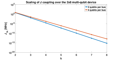
Figure 5: Exponential decay of the $J_{1k}$ coupling rate for $k=2,\ldots 8$ as measured from the first qubit $Q_{1}$ to the right in the upper rows in Figs. (3) and (4) as a function of qubit index $k$. $J_{12}$ is $-4.9\,MHz$ and $-6.1\,MHz$ in the devices in Figs. (3) and (4), respectively.

III Couplings of the Qubits to the Voltage Drives

Qubits are coupled to room temperature electronics for their readout and control. Readout and control signals pass through several amplification/attenuation stages as they travel through different stages in a dilution fridge. In between these stages they are carried over transmission lines like coaxial cables or the lines on a printed circuit board. We will content ourselves here with modeling this coupling mechanism simply by voltage sources driving the quantum chip through transmission lines(which we assume to be inifinite in extent to keep things simple here and represent them simply by resistors $Z_{0}$’s) as shown in Fig. (LABEL:fig:Cauer-circuit-with-drives). This circuit is an augmented version of the multiport canonical circuit in Fig. (LABEL:fig:Cauer-circuit) where $N_{D}$ “drive ports” are added. The drive ports are defined at positions where drive lines reach the chip (see Appendix (VIII.3) for more details on how to define the drive ports in an 3D finite-element electromagnetic simulator). They are connected to transmission lines of characteristic impedance $Z_{0}$ (typically $Z_{0}=50\Omega$) which in turn are shunted by the voltage sources $V_{d}$ for $1\leq d\leq N_{D}$. Such a simple circuit model will allow us to derive expressions for the couplings $\varepsilon_{id}$ of the qubits to voltage drives in this section. A similar analysis in Section (IV) will allow us to compute Purcell loss rates of the qubit modes due to their coupling to the drive lines.

As we show in Appendix (VIII.2) the circuit in Fig. (LABEL:fig:Cauer-circuit-with-drives) has the following Hamiltonian given in Eq. (120) in the final block-diagonalized frame corresponding to $\widetilde{\mathbf{M}}_{1}$ in Eq. (18)

$$H=\frac{1}{2}\left(\boldsymbol{q}-\mathbf{C}_{q}*\mathbf{V}_{V}\right)^{T}\left(\boldsymbol{q}-\mathbf{C}_{q}*\mathbf{V}_{V}\right)+\frac{1}{2}\boldsymbol{\phi}^{T}\widetilde{\mathbf{M}}_{1}\boldsymbol{\phi}+\mathcal{O}(\boldsymbol{\varphi}_{J}^{4})$$ (40)

where the $(N+M)\times N_{D}$ matrix $\mathbf{C}_{q}$ gives the coupling of the voltage sources $\mathbf{V}_{V}=(V_{1},\ldots,V_{N_{D}})$ to the charge degrees of freedom $\boldsymbol{q}$ of the circuit. After quantizing this Hamiltonian by introducing the harmonic mode operators $\hat{q}_{i}=-i\sqrt{\frac{\hbar}{2Z_{i}}}(\hat{b}_{i}-\hat{b}_{i}^{\dagger})$ for the qubit modes and computing the projection of $\mathbf{C}_{q}$ onto the qubit subspace one obtains the following drive term acting in the qubit subspace

$$H_{id}^{D} = i\sqrt{\frac{\hbar\omega_{i}}{2L_{i}}}\mathrm{Im}\left[Z_{i,p(d)}(\omega_{i})\right]\frac{C_{p(d)}V_{d}(\hat{b}_{i}-\hat{b}_{i}^{\dagger})}{1+i\omega_{d}Z_{0}C_{p(d)}}$$ (41)

from which we get

$$\varepsilon_{id}=\sqrt{\frac{\omega_{i}}{2\hbar L_{i}}}\mathrm{Im}\left[Z_{i,p(d)}(\omega_{i})\right]\frac{e^{i\theta_{d}}C_{p(d)}}{\sqrt{1+\omega_{d}^{2}Z_{0}^{2}C_{p(d)}^{2}}}$$ (42)

for the coupling matrix $\varepsilon_{id}$ appearing in the Hamiltonian in Eq. (1) and giving the coupling of the qubit modes to the voltage drives. Here $\theta_{d}=\frac{\pi}{2}-\arctan(\omega_{d}Z_{0}C_{p(d)})$ and $Z_{i,p(d)}$ is the impedance entry connecting the qubit port $i$ to drive port(with port index $p(d)$) corresponding to the voltage source $V_{d}$. $C_{p(d)}$ is the total capacitance shunting the $d$-th drive port, $\omega_{d}$ is the frequency of the signal driving the qubit $j$ and $Z_{0}$ is the characteristic impedance of the drive lines (typically $Z_{0}=50\Omega$). The last factor in Eq. (41) is just a voltage division factor giving how much of the drive voltage $V_{d}$ is seen across the $d$-th drive port. The factor $\mathrm{Im}\left[Z_{i,p(d)}(\omega_{i})\right]$ gives on the other hand the classical crosstalk.

III.1 The classical crosstalk and the location of the drive ports

We define the classical crosstalk as the unwanted drive the qubit $i$ experiences when we excite the device only through the drive line of the qubit $j$. For the purpose of understanding the classical cross-talk we will be only interested in the relative magnitudes of the voltages seen by different qubits and according to the analysis in Appendix (VIII.2)

$$X_{ij}=20\mathrm{log}_{10}\left(\frac{\mathrm{Im}[Z_{i,d(j)}(\omega_{i})]}{\mathrm{Im}[Z_{j,d(j)}(\omega_{j})]}\right)$$ (43)

is a good measure of the classical cross-talk in units of $dB$. Here $Z_{i,d(j)}(\omega_{i})$ is the impedance entry connecting the drive port $d(j)$ of the qubit $j$ to the qubit port $i$.

Although we have already stated in the previous sections that we defined the drive ports where the drive lines reach the chip we give a more precise description here on how we choose the locations of the drive ports. As the drive signals travel over the transmission lines towards the chip they will eventually reach the transition region (before launching onto the chip) where they will no longer see a constant impedance but a discontinuity off which some portion of the signal will be reflected back. Ideally one would like to define the drive ports at positions where this discontinuity first starts to appear. The exact positions can be determined with a TDR (time-domain reflectometry) measurement/simulation for example. In the absence of TDR information one can make a safe choice by keeping the drive ports far enough from the chip boundary. In electromagnetic finite-element simulators such ports will typically be defined as wave ports on the planes (perpendicular to the direction of propagation) in the cross-sections of the drive lines. Such a choice for the drive ports will include any crosstalk happening in the transition region (such as a spurious chip boundary mode Wirebond-Crosstalk-Martinis for example) in our crosstalk measures defined above. See Appendix (VIII.3) for more details on how to define the drive ports in electromagnetic finite-element simulators.

III.2 Example: Classical crosstalk in a multi-qubit device

Figure 6: Top: Augmented 2x8 device model with readout resonators and drive ports added. Readout resonators are represented with edges linking qubits $Q_{k}$’s to their drive ports $P_{k}$’s. Bottom: How much of the drive voltage leaks into other qubits in the upper row in the 2x8 multi-qubit device on the top figure above when only the qubit $Q_{1}$ is excited through its drive port $P_{1}$: classical crosstalk decays exponentially as a function of distance from the qubit $Q_{1}$ to the right in the first row of the circuit in the figure on the top.

In this section we augment our model for the 2x8 multi-qubit device by adding the readout resonators and the drive ports as shown on the left in Fig. (6) and apply the the formula in Eq. (43) to evaluate the cross-talk in the device. We plot $X_{1k}$ which gives the crosstalk between the drive line of the qubit $Q_{1}$ and the other qubits on the first row in Fig. (6) as a function of the qubit label $k=2,\ldots,8$ in Fig. (6).

IV Purcell Loss Rates of The Qubit Modes

Qubits are coupled to external electronics for their readout and control. In Section III we analyzed couplings of the qubits to voltage drives. The same coupling mechanism causes relaxation of the excitations in the qubit modes which is called the “Purcell Loss”. In this section we compute rates for the Purcell loss of the qubit modes we identified in the earlier sections.

As in Section (III) the coupling of the qubits to external electronics is modeled with the idealized circuit model in Fig. (LABEL:fig:Cauer-circuit-with-drives) and we will use the same coupling matrices of the formalism in Burkard that we calculated in Appendix (VIII.2) for the drive couplings. We have $N_{D}$ baths corresponding to tranmission lines of characteristic impedances $Z_{0}$’s driving the qubits as shown in Fig. (LABEL:fig:Cauer-circuit-with-drives). Assuming couplings of qubits to the lines are small, to first order in these couplings, we will assume that $T_{1}$ rates can be computed separately for each bath. The total rate will then be the sum of rates due to each line.

We start by noting that when we have only the bath due to the drive line of the voltage source $V_{d}$ with port index $p(d)$ $\mathbf{C}_{D}$ defined in Eq. (85) is a scalar $C_{p(d)}$ for $1\leq d\leq N_{D}$. Hence $\bar{\mathbf{m}}$ in Eq. (106) is

$$\bar{\mathbf{m}}_{d}=-C_{p(d)}\left(\begin{array}[]{c}\mathbf{0}_{N\times 1}\\ \mathbf{v}_{d}\end{array}\right)$$ (44)

where $\mathbf{v}_{d}=(\begin{array}[]{ccc}v_{1d}&\ldots&v_{Md}\end{array})^{T}$ is the $d$-th column of the matrix $\mathbf{V}$ corresponding to the drive line with port index $p(d)$. After the Schrieffer-Wolff transformation by Eq. (118)

$$m_{id}=C_{p(d)}\mathrm{Im}\left[Z_{i,p(d)}\left(\omega_{i}\right)\right]/\sqrt{L_{i}}$$ (45)

where $m_{id}$ is the coupling of the bath due to the $d$-th drive line to the qubit mode $i$.

We need to now compute the spectral densities of the baths corresponding to the transmission lines. $\bar{\mathbf{C}}_{Z}\left(\omega\right)$ matrix defined in Eq. (84) is also a scalar in the case of a single bath corresponding to the $d$-th drive line and is given by

$$\bar{C}_{Z,d}\left(\omega\right)=-\frac{i\omega Z_{0}}{1+i\omega C_{p(d)}Z_{0}}$$ (46)

Kernel of the bath due to the $d$-th drive line is given in Eq. (35) of Burkard as

$$K_{d}\left(\omega\right)=\frac{\bar{C}_{Z,d}\left(\omega\right)}{1+\bar{\mathbf{m}}_{d}^{T}\mathbf{C}^{-1}\bar{\mathbf{m}}_{d}\bar{C}_{Z,d}\left(\omega\right)}$$ (47)

The term $\bar{\mathbf{m}}_{d}^{T}\mathbf{C}^{-1}\bar{\mathbf{m}}_{d}$ can be evaluated in the final frame using Eq. (45) and noting that $\mathbf{C=1}$ in the final frame. Hence

$$\bar{\mathbf{m}}_{d}^{T}\mathbf{C}^{-1}\bar{\mathbf{m}}_{d}=C_{p(d)}^{2}\underset{i}{\sum}\left(\mathrm{Im}\left[Z_{i,p(d)}\left(\omega_{i}\right)\right]\right)^{2}/L_{i}$$ (48)

The spectrum of the bath is given by

$$J_{d}\left(\omega\right) = -\mathrm{Im}\left[K_{d}\left(\omega\right)\right]$$ (49)

$$= \frac{\omega Z_{0}}{1+\omega^{2}Z_{0}^{2}\left(C_{p(d)}+\bar{\mathbf{m}}_{d}^{T}\mathbf{C}^{-1}\bar{\mathbf{m}}_{d}\right)^{2}}$$

$$\simeq \frac{\omega Z_{0}}{1+\omega^{2}Z_{0}^{2}C_{p(d)}^{2}}$$

assuming $\left(\bar{\mathbf{m}}_{j}^{T}\mathbf{C}^{-1}\bar{\mathbf{m}}_{j}\right)/C_{p(d)}\ll 1$ which holds for typical parameter values and frequencies.

Finally $T_{1}$ rate of the qubit mode $i$ due to the $d$-th drive line can be calculated using Eq. (44) of Burkard

$$\frac{1}{T_{1}^{i,d}} = \frac{4}{\hbar}\left|\left\langle 0\right|m_{id}\mathbf{\hat{Q}}_{i}\left|1_{i}\right\rangle\right|^{2}J_{d}\left(\omega_{i}\right)\coth(\frac{\hbar\omega_{i}}{2k_{B}T})$$ (50)

which can be simplified assuming $\coth(\frac{\hbar\omega_{i}}{2k_{B}T})\simeq 1$ for the typical chip temperatures as

$$\frac{1}{T_{1}^{i,d}} =\frac{4}{\hbar}\left|\left\langle 0\right|m_{id}\mathbf{\hat{Q}}_{i}\left|1_{i}\right\rangle\right|^{2}J_{d}\left(\omega_{i}\right)$$

$$=\frac{2}{L_{i}}\mathrm{Im}\left[Z_{i,p(d)}\left(\omega_{i}\right)\right]^{2}\frac{\omega_{i}^{2}Z_{0}C_{p(d)}^{2}}{1+\omega_{i}^{2}Z_{0}^{2}C_{p(d)}^{2}}$$ (51)

Figure 7: Example circuit of a Transmon qubit coupled to a readout resonator which in turn coupled to external drive line of characteristic impedance $Z_{0}$. $C_{d}$ is the shunt capacitance of the drive port.

To see that Purcell rates $\frac{1}{T_{1}^{i,d}}$’s are independent of the drive port shunt capacitances $C_{p(d)}$’s we workout $Z_{i,p(d)}(\omega_{i})$ for the example circuit shown in Fig. (7). Assuming $C_{r}\gg C_{\kappa}$, $C_{q}\gg C_{c}$ and $C_{d}\gg C_{\kappa}$ one can show that

$$\mathrm{Im}\left[Z_{12}(\omega)\right]\simeq\frac{\left(\frac{C_{c}C_{\kappa}}{C_{q}C_{d}}\right)L_{r}\omega}{1-(\omega/\omega_{r})^{2}}$$ (52)

with $\omega_{r}=1/\sqrt{L_{r}C_{r}}$ and port $1$ being defined across the Josephson junction and port $2$ across $C_{d}$. So that the Purcell rate $\frac{1}{T_{1}^{i,j}}$ derived in Eq. (51) gives

$$1/T_{1} =\frac{2}{L_{q}}\mathrm{Im}\left[Z_{12}\left(\omega_{q}\right)\right]^{2}\frac{\omega_{q}^{2}Z_{0}C_{d}^{2}}{1+\omega_{q}^{2}Z_{0}^{2}C_{d}^{2}}$$

$$=\frac{2}{L_{q}}\left(\frac{C_{c}C_{\kappa}}{C_{q}C_{r}}\right)^{2}\frac{(\omega_{q}/\omega_{r})^{4}}{\left[1-(\omega_{q}/\omega_{r})^{2}\right]^{2}}\left(\frac{Z_{0}}{1+\omega_{q}^{2}Z_{0}^{2}C_{d}^{2}}\right)$$ (53)

where $\omega_{q}$ is the qubit frequency and $L_{q}$ qubit inductance. The expression in the Eq. (53) above will be independent of $C_{d}$, the total shunt capacitance of the drive port, in the limit of $\omega_{d}^{2}Z_{0}^{2}C_{d}^{2}\ll 1$ which holds for typical parameter values in the actual experiments.

One can similarly calculate coupling of the qubit to the voltage source $V_{d}$ using Eqs. (42) and (52) to get

$$\varepsilon_{12} =e^{i\theta_{2}}\sqrt{\frac{\omega_{q}}{2\hbar L_{q}}}\mathrm{Im}\left[Z_{12}(\omega_{q})\right]C_{d}$$

$$=\frac{1}{\sqrt{2\hbar Z_{q}}}\left(\frac{C_{c}C_{\kappa}}{C_{q}C_{r}}\right)\frac{(\omega_{q}/\omega_{r})^{2}}{1-(\omega_{q}/\omega_{r})^{2}}\left(\frac{e^{i\theta_{2}}}{\sqrt{1+\omega_{d}^{2}Z_{0}^{2}C_{d}^{2}}}\right)$$ (54)

where $\theta_{2}=\frac{\pi}{2}-\arctan(\omega_{d}Z_{0}C_{d})$ and $Z_{q}=\sqrt{L_{q}/C_{q}}$. Above expression for the coupling $\varepsilon_{12}$ of the qubit to its voltage source $V_{d}$ will be again independent of $C_{d}$ in the limit of $\omega_{d}^{2}Z_{0}^{2}C_{d}^{2}\ll 1$ which holds for typical parameter values.

V Expressions for the Qubit Anharmonicities and the Dispersive Shifts in the Resonator Frequencies

In this section we derive expressions for the anharmonicity $\delta_{i}$ of the qubit mode $i$ and dispersive shift $\chi_{ik}$ in the frequency $\omega_{R_{k}}$ of the resonator mode $k$ due to qubit mode $i$ using the results of Appendix (VIII.4). Anharmonicities and dispersive shifts are generated by the nonlinear terms in the expansion of the junction potentials.

From the term $H_{\beta}$ in Eq. (128) in the expansion in Eq. (126) originally given in BBQ-Yale we note the following

$$\delta_{i} = -12\beta_{iiii}$$ (55)

$$\chi_{ik} = -24\beta_{iikk}$$ (56)

Using the expression for $\beta_{pp^{\prime}qq^{\prime}}$ in Eq. (140) and Eqs. (134) and (136) we obtain

$$\delta_{i} = -E_{C}^{(i)}\left(\frac{\omega_{J_{i}}}{\omega_{i}}\right)^{2}$$ (57)

$$\chi_{ik} = -2E_{C}^{(i)}\left(\frac{\omega_{J_{i}}^{2}}{\omega_{i}\omega_{R_{k}}}\right)r_{ki}^{2}C_{i}\left(\frac{\omega_{R_{k}}^{2}}{\omega_{R_{k}}^{2}-\omega_{i}^{2}}\right)^{2}$$ (58)

From Eq. (9) we note

$$r_{ik}=\frac{2g_{ik}}{\sqrt{C_{i}\omega_{i}\omega_{R_{k}}}}$$ (59)

Hence

$$\chi_{ik} = -2E_{C}^{(i)}\left(\frac{\omega_{J_{i}}^{2}}{\omega_{i}\omega_{R_{k}}}\right)\left(\frac{4g_{ik}^{2}}{\omega_{i}\omega_{R_{k}}}\right)\left(\frac{\omega_{R_{k}}^{2}}{\omega_{R_{k}}^{2}-\omega_{i}^{2}}\right)^{2}$$ (60)

$$= 8\delta_{i}\left(\frac{g_{ik}\omega_{R_{k}}}{\omega_{R_{k}}^{2}-\omega_{i}^{2}}\right)^{2}$$

VI Conclusion & Outlook

We have analyzed superconducting quantum processors consisting of low anharmonicity transmon qubits. We have shown that the exchange coupling rates between qubits is related in a simple way to the off-diagonal entry of the multiport impedance matrix connecting the qubit ports evaluated at qubit frequencies. Qubit ports are defined across the Josephson junctions. Similarly coupling of the qubits to their drives and Purcell relaxation rates of the qubit modes are related to the entry of the multiport impedance matrix connecting the qubits and the drive ports. This gives a complete microwave description of the system in the qubit subspace. The formulas requiring only evaluation at qubit frequencies(no need for frequency sweeps and fitting) make modeling and simulation of the chips much more efficient.

Simple relations of the qubit exchange coupling rates and the couplings of the qubits to the voltage drives to the impedance response allow application of microwave engineering techniques to improve the performance of the two-qubit gates. One application could be to use microwave coupler or filtering structures to shape the response profile to reduce unwanted terms in two-qubit gates.

VII Acknowledgements

We thank Easwar Magesan and Hanhee Paik for useful discussions and Salvatore Olivadese for support with microwave simulations. DD acknowledges support from Intelligence Advanced Research Projects Activity (IARPA) under contract W911NF-16-0114.

VIII Appendix

VIII.1 Derivation of the Hamiltonian for the Canonical Multiport Cauer Circuit

Any multiport lossless impedance response can be synthesized with the canonical Cauer circuit shown in Fig. (LABEL:fig:Cauer-circuit). The Cauer circuit consists of $N$ “qubit ports” on the left shunted by the Josephson junctions in our case and $M$ internal modes synthesized as parallel $LC$ tank circuits on the right. Couplings between the ports and the internal modes are mediated by the multiport Belevitch transformers (see Newcomb for details). A purely capacitive stage (upper right) provides total shunt capacitances of the junctions. In the most general form shown in Fig. (LABEL:fig:Cauer-circuit) there is a purely inductive stage shown in the lower right corner. This stage is responsible of the purely inductive energy storage in the system. However in most of the physical situations arising with distributed electromagnetic structures this stage will be absent since any distributed inductor will always have a finite parasitic capacitance. For cases where such a stage is really necessary the degrees of freedoms associated with it can be eliminated with a Born-Oppenheimer analysis Brito .

The synthesis of the canonical Cauer circuit in Fig. (LABEL:fig:Cauer-circuit) proceeds as follows: first we do the eigendecomposition of the residue at DC $\mathbf{A}_{0}$ in Eq. (7)

$$\mathbf{A}_{0}=\mathbf{U}\mathbf{C}_{0}^{-1}\mathbf{U}^{T}$$ (61)

where $\mathbf{U}$ is the $N\times N$ orthonormal matrix holding the eigenvectors of $\mathbf{A}_{0}$ and $\mathbf{C}_{0}$ is the diagonal matrix with entries $\left(C_{1},\ldots,C_{N}\right)$, inverses of eigenvalues of $\mathbf{A}_{0}$. Entries of $\mathbf{U}$ are the turns ratios of the multiport Belevitch transformer corresponding to the purely capacitive stage in Fig. (LABEL:fig:Cauer-circuit). In the case of no direct electrostatic interaction between the qubit port terminals $\mathbf{U}$ will be simply the identity matrix.

For the internal modes of frequency $\omega_{R_{k}}=1/\sqrt{L_{R_{k}}C_{R_{k}}}$ we choose a characteristic impedance of $Z_{0}=1/\omega_{R_{k}}$ that will make all $C_{R_{k}}=1$ for $1\leq k\leq M$. There is a freedom in the choice of this characteristic impedance; this choice should have no effect on the physical coupling rates. With this choice we have $L_{R_{k}}=1/\omega_{R_{k}}^{2}$. Then with $\mathbf{A}_{k}$’s being rank-1 matrices DDV and with our choice of $C_{R_{k}}=1$

$$\mathbf{A}_{k}=r_{k}^{T}r_{k}$$ (62)

where $r_{k}$ is the row-vector $r_{k}=(r_{k1},\ldots,r_{kN})$ for $1\leq k\leq M$. $r_{k}$’s constitute rows of turn ratios of the multiport Belevitch transformer matrix $\mathbf{R}$ connecting the internal modes to the ports.

The final purely inductive stage can be synthesized in a similar way to the purely capacitive DC stage with a eigendecomposition of the $\mathbf{A}_{\infty}$ matrix

$$\mathbf{A}_{\infty}=\mathbf{T}^{T}\mathbf{L}_{\infty}\mathbf{T}$$ (63)

with $\mathbf{T}$ being the orthonormal matrix holding the eigenvectors and the diagonal matrix $\mathbf{L}_{\infty}$ holding the inductances $(L_{1}^{\infty},\ldots,L_{N}^{\infty})$.

Using the lumped element circuit quantization method in Burkard together with a technique to handle multiport Belevitch transformers Solgun we can identify the degrees of freedom in the Cauer circuit in Fig. (LABEL:fig:Cauer-circuit) and write an equation of motion. The effective fundamental loop matrix defined in Eq. (21) of Burkard is

$$\mathbf{F}_{C}=\left(\begin{array}[]{c}\mathbf{U}\\ -\mathbf{R}\mathbf{U}\end{array}\right)$$ (64)

The Hamiltonian is

$$\mathcal{H}=\frac{1}{2}\mathbf{Q}^{T}\mathbf{C}^{-1}\mathbf{Q}+\frac{1}{2}\mathbf{\Phi}^{T}\mathbf{M}_{0}\mathbf{\Phi}-\stackrel{{\scriptstyle[}}{{i}}=1]{N}{\sum}E_{J_{i}}\cos\left(\varphi_{J_{i}}\right)$$ (65)

where $\mathbf{\Phi}=(\Phi_{J_{1}},\ldots,\Phi_{J_{N}},\Phi_{R_{1}},\ldots,\Phi_{R_{M}})^{T}$ being the flux coordinate vector. $\varphi_{J_{i}}$ is the phase of the junction $i$ related to the flux across it by the Josephson relation $\Phi_{J_{i}}=\frac{\mathrm{\Phi}_{0}}{2\pi}\varphi_{J_{i}}$, for $1\leq i\leq N$. $\Phi_{R_{k}}$ is the flux across the inductor of the internal mode $k,$ $1\leq k\leq M$. $E_{J_{i}}$ is the Josephson energy of junction $i$ related to its inductance $L_{J_{i}}$ by $E_{J_{i}}=\left(\frac{\mathrm{\Phi}_{0}}{2\pi}\right)^{2}\frac{1}{L_{J_{i}}}$. The capacitance matrix $\mathbf{C}$ is given by

$$\mathbf{C} =\mathbf{F}_{C}\mathbf{C}_{0}\mathbf{F}_{C}^{T}+\mathbf{C}_{R}$$

$$=\left(\begin{array}[]{cc}\mathbf{U}\mathbf{C}_{0}\mathbf{U}^{T}&-\mathbf{U}\mathbf{C}_{0}\mathbf{U}^{T}\mathbf{R}^{T}\\ -\mathbf{R}\mathbf{U}\mathbf{C}_{0}\mathbf{U}^{T}&\mathbf{C}_{R}+\mathbf{R}\mathbf{U}\mathbf{C}_{0}\mathbf{U}^{T}\mathbf{R}^{T}\end{array}\right)$$ (68)

The capacitance matrix becomes

$$\mathbf{C}=\left(\begin{array}[]{cc}\mathbf{C}_{0}&-\mathbf{C}_{0}\mathbf{R}^{T}\\ -\mathbf{R}\mathbf{C}_{0}&\mathbf{1}_{M\times M}+\mathbf{R}\mathbf{C}_{0}\mathbf{R}^{T}\end{array}\right)$$ (69)

in the absence of direct electrostatic dipole interactions between the ports since $\mathbf{U}$ is the identity matrix in that case and with our choice of $\mathbf{C}_{R}=\mathbf{1}_{M\times M}$ for the capacitances of the internal modes.

$\mathbf{M}_{0}$ is the diagonal matrix holding the inverses of the inductances of the internal modes on its diagonal

$$\mathbf{M}_{0}=\left(\begin{array}[]{cccc}\mathbf{0}_{N\times N}&&&\mathbf{0}\\ &1/L_{R_{1}}\\ &&\ddots\\ \mathbf{0}&&&1/L_{R_{M}}\end{array}\right)$$ (70)

VIII.2 Derivation of the Couplings Rates of the Qubits to the Voltage Drives

In this appendix we augment the canonical Cauer circuit in Fig. (LABEL:fig:Cauer-circuit) by including the drive lines as shown in Fig. (LABEL:fig:Cauer-circuit-with-drives). We added $N_{D}$ drive lines hence $N_{D}$ more ports. Drive line for the qubit $i$ consists of the voltage source $V_{d(i)}$ driving the transmission line of characteristic impedance $Z_{0}$ whose other end is connected to the drive port $d(i)$ (Here we are assuming that $d(i)$ is the index number of the drive port corresponding to the qubit $i$). Synthesis of such a circuit from an impedance matrix $\mathbf{Z}(\omega)$ proceeds as described in the previous section, this time with $N+N_{D}$ ports.

Again using the method in Burkard we obtain the following Hamiltonian for the augmented Cauer circuit in Fig. (LABEL:fig:Cauer-circuit-with-drives)

$$\mathcal{H}=\frac{1}{2}(\mathbf{Q}-\mathbf{C}_{Q}\ast\mathbf{V}_{V})^{T}\mathbf{C}^{-1}(\mathbf{Q}-\mathbf{C}_{Q}\ast\mathbf{V}_{V})+\frac{1}{2}\mathbf{\Phi}^{T}\mathbf{M}_{0}\mathbf{\Phi}-\stackrel{{\scriptstyle[}}{{i}}=1]{N}{\sum}E_{J_{i}}\cos\left(\varphi_{J_{i}}\right)$$ (71)

where as in the previous section $\mathbf{\Phi}=\left(\Phi_{J_{1}},\ldots,\Phi_{J_{N}},\Phi_{R_{1}},\ldots,\Phi_{R_{M}}\right)^{T}$ is the flux coordinate vector. The capacitance matrix $\mathbf{C}$ is given by

$$\mathbf{C}=\mathbf{F}_{C}\mathbf{C}_{S}\mathbf{F}_{C}^{T}+\mathbf{C}_{R}$$ (72)

where $\mathbf{C}_{S}$ is the diagonal matrix holding the total shunt capacitances seen at the ports

$$\mathbf{C}_{S}=\left(\begin{array}[]{cc}\mathbf{C}_{0}&\mathbf{0}\\ \mathbf{0}&\mathbf{C}_{D}\end{array}\right)$$ (73)

where $\mathbf{C}_{0}$ and $\mathbf{C}_{D}$ are $N\times N$ and $N_{D}\times N_{D}$ diagonal matrices holding total capacitances shunting the qubit and drive ports, respectively such that

$$\mathbf{C}_{0}=\left(\begin{array}[]{ccc}C_{1}&&\mathbf{0}\\ &\ddots\\ \mathbf{0}&&C_{N}\end{array}\right)$$ (74)

$$\mathbf{C}_{D}=\left(\begin{array}[]{ccc}C_{N+1}&&\mathbf{0}\\ &\ddots\\ \mathbf{0}&&C_{N+N_{D}}\end{array}\right)$$ (75)

where capacitances $(C_{1},\ldots,C_{N},C_{N+1},\ldots,C_{N+N_{D}})$ are shown in Fig.LABEL:fig:Cauer-circuit-with-drives in the purely capacitive stage coupled to the rest of the circuit with the multiport Belevitch transformer $\mathbf{U}$. $\mathbf{C}_{R}$ is again the identity matrix in the resonator subspace and neglecting any electrostatic dipole interaction between the ports (i.e. $\mathbf{U}=\mathbf{1}$) the fundamental loop matrix $\mathbf{F}_{C}$ is given by

$$\mathbf{F}_{C}=\left(\begin{array}[]{cc}\mathbf{1}_{N\times N}&\mathbf{0}_{N\times N_{D}}\\ -\mathbf{R}&-\mathbf{V}\end{array}\right)$$ (76)

where $\mathbf{F}_{C}$, $\mathbf{R}$ and $\mathbf{V}$ are $(N+M)\times(N+N_{D})$ , $(M\times N)$ and $(M\times N_{D})$ matrices, respectively. Matrices $\mathbf{R}$ and $\mathbf{V}$ are multiport Belevitch transformer matrices (with turn ratio entries $r_{ki}$ and $v_{kd}$ as shown in Fig. (LABEL:fig:Cauer-circuit-with-drives) for $1\leq k\leq M$, $1\leq i\leq N$ and $1\leq d\leq N_{D}$) mediating the couplings of the internal modes to the qubits and the voltage sources, respectively. The diagonal matrix $\mathbf{M}_{0}$ again holds the inverses of the inductances of the internal modes on its diagonal

$$\mathbf{M}_{0}=\left(\begin{array}[]{cccc}\mathbf{0}_{N\times N}&&&\mathbf{0}\\ &1/L_{R_{1}}\\ &&\ddots\\ \mathbf{0}&&&1/L_{R_{M}}\end{array}\right)$$ (77)

$\mathbf{V}_{V}=(V_{1},\ldots,V_{N_{D}})$ is the vector of voltage sources and $\ast$ is the time convolution operator. $\mathbf{C}_{Q}$ is the $(N+M)\times N_{D}$ matrix coupling the voltage source $\mathbf{V}_{V}$ vector to the charge coordinates $\mathbf{Q}$ and is given by

$$\mathbf{C}_{Q}=\mathrm{\mathbf{C}}_{V}+\mathcal{C}_{V}$$ (78)

As we will show below $\mathrm{\mathbf{C}}_{V}$ is frequency independent whereas $\mathcal{C}_{V}$ is non-zero only for AC voltage drives. $\mathrm{\mathbf{C}}_{V}$ is given in Eq. (23) in Burkard as

$$\mathrm{\mathbf{C}}_{V}=\mathbf{F}_{C}\mathbf{C}_{S}\mathbf{F}_{VC}^{T}$$ (79)

where the loop matrix $\mathbf{F}_{VC}$ is given by

$$\mathbf{F}_{VC}=\left(\begin{array}[]{cc}\mathbf{0}_{N\times N}&\mathbf{1}_{N\times N_{D}}\end{array}\right)$$ (80)

$\mathcal{C}_{V}(\omega)$ is given in Eq. (7.25) of Solgun which is an extension of Eq. (23) of Burkard to AC voltage sources

$$\mathcal{C}_{V}(\omega)=\bar{\mathbf{m}}\bar{\mathbf{C}}_{Z}\bar{\mathbf{m}}_{V}^{T}$$ (81)

where from Eqs. (7.19-7.21) in Solgun

$$\bar{\mathbf{m}} = \mathbf{F}_{C}\mathbf{C}_{S}\mathbf{F}_{ZC}^{T}$$ (82)

$$\bar{\mathbf{m}}_{V} = \mathbf{F}_{VC}\mathbf{C}_{S}\mathbf{F}_{ZC}^{T}$$ (83)

$$\bar{\mathbf{C}}_{Z}(\omega) = -i\omega\mathbf{Z}_{0}\left[\mathbf{1}+i\omega\mathbf{F}_{ZC}\mathbf{C}_{S}\mathbf{F}_{ZC}^{T}\mathbf{Z}_{0}\right]^{-1}$$ (84)

Here $\mathbf{F}_{ZC}=\mathbf{F}_{VC}$ given in Eq. (80) and $\mathbf{Z}_{0}$ is the $N_{D}\times N_{D}$ matrix giving the multiport impedance seen at the drive ports looking into the environment away from the chip and is simply the diagonal matrix consisting of diagonal entries $Z_{0}$’s.

We observe that $\mathrm{\mathbf{C}_{V}=\bar{\mathbf{m}}}$ since $\mathbf{F}_{VC}=\mathbf{F}_{ZC}$. Noting

$$\mathbf{F}_{ZC}\mathbf{C}_{S}\mathbf{F}_{ZC}^{T}=\mathbf{C}_{D}$$ (85)

we write

$$\bar{\mathbf{C}}_{Z}(\omega)=-i\omega\mathbf{Z}_{0}\left[\mathbf{1}+i\omega\mathbf{C}_{D}\mathbf{Z}_{0}\right]^{-1}$$ (86)

We now work out $\bar{\mathbf{m}}$ using Eqs. (82), (73), (76), (80) and noting $\mathbf{F}_{ZC}=\mathbf{F}_{VC}$

$$\bar{\mathbf{m}} = \mathbf{F}_{C}\mathbf{C}_{S}\mathbf{F}_{ZC}^{T}$$ (92)

$$= \left(\begin{array}[]{cc}\mathbf{1}&\mathbf{0}\\ -\mathbf{R}&-\mathbf{V}\end{array}\right)\left(\begin{array}[]{cc}\mathbf{C}_{0}&\mathbf{0}\\ \mathbf{0}&\mathbf{C}_{D}\end{array}\right)\left(\begin{array}[]{cc}\mathbf{0}&\mathbf{1}\end{array}\right)^{T}$$

$$= \left(\begin{array}[]{c}\mathbf{0}\\ -\mathbf{V}\mathbf{C}_{D}\end{array}\right)$$ (95)

Applying the capacitance rescaling $\mathbf{\Phi}_{J}\rightarrow\mathbf{C}_{0}^{1/2}\mathbf{\Phi}_{J}$ and the transformation in Eq. (12) to $\bar{\mathbf{m}}$ in Eq. (95)

$$\bar{\mathbf{m}}\rightarrow\mathbf{T}^{t}\left(\begin{array}[]{cc}\mathbf{C}_{0}^{-1/2}&\mathbf{0}\\ \mathbf{0}&\mathbf{1}\end{array}\right)\bar{\mathbf{m}}$$ (96)

we get

$$\bar{\mathbf{m}} = \left(\begin{array}[]{cc}\mathbf{1}&\mathbf{0}\\ \mathbf{R}\mathbf{C}_{0}^{1/2}&\mathbf{1}\end{array}\right)\left(\begin{array}[]{cc}\mathbf{C}_{0}^{-1/2}&\mathbf{0}\\ \mathbf{0}&\mathbf{1}\end{array}\right)\left(\begin{array}[]{c}\mathbf{0}\\ -\mathbf{V}\end{array}\right)\mathbf{C}_{D}$$ (103)

$$= \left(\begin{array}[]{c}\mathbf{0}\\ -\mathbf{V}\mathbf{C}_{D}\end{array}\right)$$ (106)

We note that $\bar{\mathbf{m}}$ is unaffected by this transformation. Since $\mathrm{\mathbf{C}_{V}=\bar{\mathbf{m}}}$ we have after the transformations

$$\mathrm{\mathbf{C}}_{V}=\left(\begin{array}[]{c}\mathbf{0}\\ -\mathbf{V\mathbf{C}}_{D}\end{array}\right)$$ (107)

Noting

$$\bar{\mathbf{m}}_{V} = \mathbf{F}_{VC}\mathbf{C}\mathbf{F}_{ZC}^{T}$$ (108)

$$= \mathbf{F}_{ZC}\mathbf{C}\mathbf{F}_{ZC}^{T}$$

$$= \mathbf{C}_{D}$$

we can write Eq. (81) as

$$\mathcal{C}_{V}(\omega) = \bar{\mathbf{m}}\bar{\mathbf{C}}_{Z}\bar{\mathbf{m}}_{V}^{T}$$ (111)

$$= \left(\begin{array}[]{c}\mathbf{0}\\ \mathbf{V}\end{array}\right)\widetilde{\mathbf{C}}_{Z}(\omega)$$

where we defined the $N_{D}\times N_{D}$ matrix

$$\widetilde{\mathbf{C}}_{Z}\left(\omega\right)=i\omega\mathbf{C}_{D}\mathbf{Z}_{0}\left[\mathbf{1}+i\omega\mathbf{C}_{D}\mathbf{Z}_{0}\right]^{-1}\mathbf{C}_{D}$$ (112)

We have one final step to do, that is to apply the Schrieffer-Wolff transformation to $\mathrm{\mathbf{C}}_{V}$ and $\mathcal{C}_{V}(\omega)$ such that

$$\mathrm{\mathbf{C}}_{V} \rightarrow \exp(-\mathbf{S})\mathrm{\mathbf{C}}_{V}$$ (113)

$$\mathcal{C}_{V}(\omega) \rightarrow \exp(-\mathbf{S})\mathcal{C}_{V}(\omega)$$ (114)

Using Eqs. (B.4) and (B.12a) of Winkler and noting block structures of matrices $\mathbf{S}$, $\mathrm{C}_{V}$ and $\mathcal{C}_{V}(\omega)$ we first define the following $(N+M)\times N_{D}$ matrix $\mathbf{D}$ having the $\left(i,d\right)$-th entry $D_{id}$ in the qubit subspace:

$$D_{id} = \left[\exp(-\mathbf{S})\left(\begin{array}[]{c}\mathbf{0}\\ -\mathbf{V}\end{array}\right)\right]_{id}$$

$$= -\underset{k}{\sum}\left(\mathbf{M}_{1}\right)_{ik}\frac{v_{kd}}{\omega_{i}^{2}-\omega_{R_{k}}^{2}}$$

$$=- \omega_{i}^{2}C_{i}^{1/2}\underset{k}{\sum}\frac{r_{ki}v_{kd}}{\omega_{i}^{2}-\omega_{R_{k}}^{2}}$$

$$= -\omega_{i}^{2}C_{i}^{1/2}\underset{k}{\sum}\frac{[\mathbf{A}_{k}]_{i,p(d)}}{\omega_{i}^{2}-\omega_{R_{k}}^{2}}$$

$$= \omega_{i}C_{i}^{1/2}\mathrm{Im}\left[Z_{i,p(d)}(\omega_{i})\right]$$

$$= \mathrm{Im}\left[Z_{i,p(d)}\left(\omega_{i}\right)\right]/\sqrt{L_{i}}$$ (118)

where $v_{kd}$ is the $\left(k,d\right)$-th entry of $\mathbf{V}$ for $1\leq k\leq M$ and $1\leq d\leq N_{D}$. In the third line above we used Eq. (21) to replace $\left(\mathbf{M}_{1}\right)_{ik}$ with $\omega_{i}^{2}C_{i}^{1/2}r_{ki}$ and in the fourth line $[\mathbf{A}_{k}]_{i,p(d)}=r_{ki}v_{kd}$ where $[\mathbf{A}_{k}]_{i,p(d)}$ is the entry of the residue matrix $\mathbf{A}_{k}$ in the impedance expansion in Eq. (7) for the circuit in Fig. (LABEL:fig:Cauer-circuit-with-drives) connecting the qubit port $i$ to drive port (with port index $p(d)$) corresponding to the voltage source $V_{d}$. Hence $\mathbf{C}_{Q}$ transforms to

$$\mathbf{C}_{Q}\rightarrow\mathbf{C}_{q}=\mathbf{D}\left(\mathbf{C}_{D}-\widetilde{\mathbf{C}}_{Z}(\omega)\right)$$ (119)

Then one can write the following Hamiltonian in the final frame corresponding to $\widetilde{\mathbf{M}}_{1}$ in Eq. (17)

$$H=\frac{1}{2}\left(\boldsymbol{q}-\mathbf{C}_{q}*\mathbf{V}_{V}\right)^{T}\left(\boldsymbol{q}-\mathbf{C}_{q}*\mathbf{V}_{V}\right)+\frac{1}{2}\boldsymbol{\phi}^{T}\widetilde{\mathbf{M}}_{1}\boldsymbol{\phi}+\mathcal{O}(\boldsymbol{\varphi}_{J}^{4})$$ (120)

with the $(N+M)\times N_{D}$ matrix $\mathbf{C}_{q}$ giving the couplings of the voltage drives $\mathbf{V}_{V}$ to the momentum degrees of freedom $\boldsymbol{q}$ in the final frame. After quantization by introducing $\hat{q}_{i}=-i\sqrt{\frac{\hbar}{2Z_{i}}}(\hat{b}_{i}-\hat{b}_{i}^{\dagger})$ and noting that the characteristic impedance $Z_{i}$ of the qubit mode $i$ is $Z_{i}=1/\omega_{i}$ we get the drive term on qubit $i$ due to voltage source $V_{d}$

$$H_{id}^{D}=i\sqrt{\frac{\hbar\omega_{i}}{2}}\left[\mathbf{C}_{q}(\omega_{d})\right]_{i,d}V_{d}(\hat{b}_{i}-\hat{b}_{i}^{\dagger})$$ (121)

where $\left[\mathbf{C}_{q}(\omega_{d})\right]_{i,d}$ is $(i,d)$-th entry of $\mathbf{C}_{q}$ evaluated at the frequency $\omega_{d}$ (We assumed that $V_{d}$ is a single-tone sinusoidal voltage drive at frequency $\omega_{d}$). In the case of zero off-chip crosstalk $\widetilde{\mathbf{C}}_{Z}$ is diagonal and using Eqs. (118) and (119) we have

$$H_{id}^{D} = i\sqrt{\frac{\hbar\omega_{i}}{2L_{i}}}\mathrm{Im}\left[Z_{i,p(d)}(\omega_{i})\right]\frac{C_{p(d)}V_{d}(\hat{b}_{i}-\hat{b}_{i}^{\dagger})}{1+i\omega_{d}Z_{0}C_{p(d)}}$$ (122)

where $C_{p(d)}$ is the $d$-th diagonal entry of $\mathbf{C}_{D}$. We note here that $\varepsilon_{id}$ in Eq. (1) is

$$\varepsilon_{id}=i\sqrt{\frac{\omega_{i}}{2\hbar L_{i}}}\mathrm{Im}\left[Z_{i,p(d)}(\omega_{i})\right]\left(\frac{C_{p(d)}}{1+i\omega_{d}Z_{0}C_{p(d)}}\right)$$ (123)

which can be also written as

$$\varepsilon_{id}=\sqrt{\frac{\omega_{i}}{2\hbar L_{i}}}\mathrm{Im}\left[Z_{i,p(d)}(\omega_{i})\right]\frac{e^{i\theta_{d}}C_{p(d)}}{\sqrt{1+\omega_{d}^{2}Z_{0}^{2}C_{p(d)}^{2}}}$$ (124)

with $\theta_{d}=\frac{\pi}{2}-\arctan(\omega_{d}Z_{0}C_{p(d)})$.

One can then define the following quantity (in units of $dB$) as a measure of classical on-chip cross-talk on qubit $i$ while driving qubit $j$

$$X_{ij} = 20\mathrm{log}_{10}\left(\sqrt{\frac{\omega_{i}L_{J_{j}}}{\omega_{j}L_{J_{i}}}}\right)+20\mathrm{log}_{10}\left(\frac{\mathrm{Im}[Z_{i,d(j)}(\omega_{i})]}{\mathrm{Im}[Z_{j,d(j)}(\omega_{j})]}\right)$$ (125)

$$\simeq 20\mathrm{log}_{10}\left(\frac{\mathrm{Im}[Z_{i,d(j)}(\omega_{i})]}{\mathrm{Im}[Z_{j,d(j)}(\omega_{j})]}\right)$$

In the definition of the above crosstalk measure we neglected the term involving qubit frequencies and junction inductances assuming similar values.

VIII.3 Defining the Qubit Ports and the Drive Ports in the 3D Finite-Element Electromagnetic Simulators

In the main text we described in words how to define the qubit ports and the drive ports. In this appendix we illustrate the definition of the ports with the help of the 3D model of a 7-Qubit device in HFSS HFSS as shown in Fig. (LABEL:fig:Port-Definitions) (HFSS is a high-frequency finite-element electromagnetics simulator). The device consists of a quantum chip (shown in light blue in the middle) packaged together with a PCB (Printed Circuit Board) supporting transmission lines carrying the drive and readout signals to/from the chip. The metallization of the PCB is shown in orange and the dielectric of the PCB is shown in burgundy color in Fig. (LABEL:fig:Port-Definitions). For the definition of the drive ports we choose a bounding box enclosing the quantum chip and some part of the PCB. The boundaries of the box should be chosen far enough from the chip. As we stated in the main text the exact position of this boundary can be determined with a TDR (Time-Domain Reflectometry) experiment/simulation. Ideally we would like to put the boundary at the location where signals traveling in the transmission lines of the PCB start to see a change in the constant impedance of the transmission lines. This happens where the signals enter the discontinuity region between the PCB and the chip. The drive ports are usually defined as wave ports in HFSS to which it is assumed that a constant impedance transmission line is connected. An example of a drive port is shown in the sub-figure (d) in Fig. (LABEL:fig:Port-Definitions) as the magenta rectangle on one of the side surfaces of the bounding box shown in sub-figure (b) in Fig. (LABEL:fig:Port-Definitions).

Qubit Ports are defined as lumped ports in HFSS. This is shown in sub-figures (e) and (f) in Fig. (LABEL:fig:Port-Definitions). The qubit port is the small magenta square shown in sub-figure (f) in Fig. (LABEL:fig:Port-Definitions). HFSS puts a differential excitation between the edges of this square touching the junction terminals.

VIII.4 Expansion of the junction potentials

Qubit anharmonicities and dispersive shifts between the modes are obtained after including the nonlinear terms in the junction potentials. For this we use the normal ordered expansion as given in Eq. (16) of BBQ-Yale :

$$H=H_{0}+H_{\gamma}+H_{\beta}+\mathcal{O}(\hat{\varphi}_{J}^{6})$$ (126)

with

$$H_{\gamma} = -\underset{pp^{\prime}}{\sum}\gamma_{pp^{\prime}}(2\hat{a}_{p}^{\dagger}a_{p^{\prime}}+\hat{a}_{p}\hat{a}_{p^{\prime}}+\hat{a}_{p}^{\dagger}\hat{a}_{p^{\prime}}^{\dagger})$$ (127)

$$H_{\beta} = \underset{pp^{\prime}qq^{\prime}}{-\sum}\beta_{pp^{\prime}qq^{\prime}}(6\hat{a}_{p}^{\dagger}\hat{a}_{p^{\prime}}^{\dagger}\hat{a}_{q}\hat{a}_{q^{\prime}}+4\hat{a}_{p}^{\dagger}\hat{a}_{p^{\prime}}^{\dagger}\hat{a}_{q}^{\dagger}\hat{a}_{q^{\prime}}+4\hat{a}_{p}^{\dagger}\hat{a}_{p^{\prime}}\hat{a}_{q}\hat{a}_{q^{\prime}}+\hat{a}_{p}\hat{a}_{p^{\prime}}\hat{a}_{q}\hat{a}_{q^{\prime}}+\hat{a}_{p}^{\dagger}\hat{a}_{p^{\prime}}^{\dagger}\hat{a}_{q}^{\dagger}\hat{a}_{q^{\prime}}^{\dagger})$$ (128)

where $H_{0}$ is the linearized part of the Hamiltonian obtained after replacing the junctions with linear inductors, $p$, $p^{\prime}$, $q$, $q^{\prime}$ are the labels of the harmonic modes in the basis defined by $H_{0}$ and $\hat{a}_{p}(\hat{a}_{p}^{\dagger})$ is the annihilation(creation) operator of the mode $p$. This expansion was originally done in BBQ-Yale in a diagonal frame whereas here we will expand in the block-diagonalized frame corresponding to the matrix $\widetilde{\mathbf{M}}_{1}$ in Eq. (17). That is the linearized Hamiltonian $H_{0}$ in our case is the linear part of the Hamiltonian given in Eq. (18)

$$H_{0}=\frac{1}{2}\boldsymbol{q}^{T}\boldsymbol{q}+\frac{1}{2}\boldsymbol{\phi}^{T}\widetilde{\mathbf{M}}_{1}\boldsymbol{\phi}$$ (129)

In that frame the capacitance matrix is unity and the coordinate vector holds the flux variables $\boldsymbol{\phi}=(\phi_{1}\ldots\phi_{N+M})$. The first $N$ coordinates correspond to qubit modes and the last $M$ coordinates correspond to the resonator modes(or internal modes). $\boldsymbol{q}$ is the vector of momenta conjugate to coordinates $\boldsymbol{\phi}$ . The flux operators $\boldsymbol{\phi}$ of the modes in the final frame can be related to the fluxes $\mathbf{\Phi}$ in the initial frame by the total coordinate transformation

$$\mathbf{\Phi}=\left(\begin{array}[]{c}\mathbf{\Phi}_{J}\\ \mathbf{\Phi}_{R}\end{array}\right)=\left(\begin{array}[]{cc}\mathbf{C}_{0}^{-1/2}&\mathbf{0}\\ \mathbf{0}&\mathbf{1}\end{array}\right)\boldsymbol{\alpha}\boldsymbol{\phi}$$ (130)

where $\boldsymbol{\alpha}=\mathbf{T}\exp(\mathbf{S})$; matrices $\mathbf{C}_{0}$, $\mathbf{T}$, $\mathbf{S}$ are defined in the text in Eqs. (9), (12) and (17), respectively. In particular

$$\mathbf{\Phi}_{J} = \left(\begin{array}[]{cc}\mathbf{C}_{0}^{-1/2}&\mathbf{0}_{N\times M}\end{array}\right)\boldsymbol{\alpha}\boldsymbol{\phi}$$ (132)

where $\mathbf{\Phi}_{J}=(\Phi_{J_{1}}\ldots\Phi_{J_{N}})^{T}$ is the vector of fluxes across the Josephson junctions. Hence

$$\Phi_{J_{i}}=\frac{1}{\sqrt{C_{i}}}\left[\stackrel{{\scriptstyle[}}{{j}}=1]{N}{\sum}\alpha_{ij}\phi_{j}+\stackrel{{\scriptstyle[}}{{k}}=1]{M}{\sum}\alpha_{i,k+N}\phi_{k}\right]$$ (133)

where indices $i$, $j$ label qubit modes and $k$ labels resonator modes with $1\leq i,j\leq N$ and $1\leq k\leq M$. The $(N+M)\times(N+M)$ matrix $\boldsymbol{\alpha}$ has the entries

$$\alpha_{ii} = 1-\mathrm{Im}[Z_{ii}^{(AC)}(\omega_{i})]/Z_{i}$$ (134)

$$\alpha_{ij} = -\mathrm{Im}[Z_{ij}(\omega_{i})]/Z_{i}$$ (135)

$$\alpha_{i,k+N} = r_{ki}C_{i}^{1/2}\left(\frac{\omega_{R_{k}}^{2}}{\omega_{R_{k}}^{2}-\omega_{i}^{2}}\right)$$ (136)

In the dispersive regime we have $\left|\mathrm{Im}[Z_{ii}^{(AC)}(\omega_{i})]/Z_{i}\right|\ll 1$ hence $\alpha_{ii}\simeq 1$, $\left|\alpha_{ij}\right|=\left|\mathrm{Im}[Z_{ij}(\omega_{i})]/Z_{i}\right|\ll 1$ for $1\leq i,j\leq N$ and $\left|\alpha_{i,k+N}\right|=\left|r_{ki}C_{i}^{1/2}\left(\frac{\omega_{R_{k}}^{2}}{\omega_{R_{k}}^{2}-\omega_{i}^{2}}\right)\right|\ll 1$ for $1\leq k\leq M$ hence we can treat $\alpha_{ij}$ and $\alpha_{i,k+N}$’s as small parameters. $\mathrm{Im}[Z_{ii}^{(AC)}(\omega_{i})]=\stackrel{{\scriptstyle[}}{{k}}=1]{M}{\sum}\frac{\left[A_{k}\right]_{ii}\omega_{i}}{\omega_{R_{k}}^{2}-\omega_{i}^{2}}$ is the AC part of $\mathrm{Im}[Z_{ii}(\omega_{i})]$.

Similarly resonator fluxes $\mathbf{\Phi}_{R}=(\Phi_{R_{1}},\ldots,\Phi_{R_{M}})$ in the initial frame can also be related to the flux coordinates $\boldsymbol{\phi}$ in the final frame

$$\Phi_{R_{k}}=\stackrel{{\scriptstyle[}}{{i}}=1]{N}{\sum}\alpha_{k+N,i}\phi_{i}+\phi_{k}$$ (137)

where

$$\alpha_{k+N,i} = r_{ki}C_{i}^{1/2}\left(\frac{\omega_{i}^{2}}{\omega_{i}^{2}-\omega_{R_{k}}^{2}}\right)$$ (138)

and $\alpha_{k+N,k+N}=1$ for $1\leq k\leq M$ by Eq. (137).

The expression for the coefficients $\beta_{pp^{\prime}qq^{\prime}}$ is given in BBQ-Yale as

$$\beta_{pp^{\prime}qq^{\prime}}=\stackrel{{\scriptstyle[}}{{s}}=1]{N}{\sum}\frac{e^{2}}{24L_{J}^{(s)}}\xi_{sp}\xi_{sp^{\prime}}\xi_{sq}\xi_{sq^{\prime}}$$ (139)

where $L_{J}^{(s)}$ is the inductance of the $s^{th}$ junction. In our case $\xi_{sp}=\alpha_{sp}/\sqrt{\omega_{p}}$ after the introduction of mode operators as $\hat{\phi}_{p}=\sqrt{\frac{\hbar Z_{p}}{2}}(\hat{a}_{p}+\hat{a}_{p}^{\dagger})$ in the final frame with characteristic impedance $Z_{p}=1/\omega_{p}$ one gets

$$\beta_{pp^{\prime}qq^{\prime}}=\stackrel{{\scriptstyle[}}{{s}}=1]{N}{\sum}\frac{E_{C}^{(s)}}{12}\omega_{J_{s}}^{2}\left(\omega_{p}\omega_{p^{\prime}}\omega_{q}\omega_{q^{\prime}}\right)^{-1/2}\alpha_{sp}\alpha{}_{sp^{\prime}}\alpha{}_{sq}\alpha_{sq^{\prime}}$$ (140)

where $E_{C}^{(s)}=\frac{e^{2}}{2C_{s}}$ and $\omega_{J_{s}}=1/\sqrt{L_{J_{s}}C_{s}}$.

$\gamma_{pp^{\prime}}$ is given in BBQ-Yale as

$$\gamma_{pp^{\prime}}=6\stackrel{{\scriptstyle[}}{{q}}=1]{N+M}{\sum}\beta_{qqpp^{\prime}}$$ (141)

We observe that $\gamma_{pp}$ is of order $E_{C}^{(s)}$. Since $E_{C}^{(s)}$ is already small compared to qubit frequencies we will be only interested in the first order expansion of $\gamma_{pp^{\prime}}$ in the small parameters $\alpha_{ij}$’s and $\alpha_{i,k+N}$’s. Then we can write the diagonal entries as

$$\gamma_{ii} \simeq 6\beta_{iiii}$$ (142)

$$\simeq \frac{E_{C}^{(i)}\omega_{J_{i}}^{2}}{2\omega_{i}^{2}}\alpha_{ii}^{2}$$

The off-diagonal entry $\gamma_{ij}$ between qubit modes $i$ and $j$ is

$$\gamma_{ij} \simeq 6(\beta_{iiij}+\beta_{jjij})$$ (143)

$$\simeq \frac{E_{C}^{(i)}\omega_{J_{i}}^{2}}{2\omega_{i}}\frac{\alpha_{ii}\alpha_{ij}}{\sqrt{\omega_{i}\omega_{j}}}+\frac{E_{C}^{(j)}\omega_{J_{j}}^{2}}{2\omega_{j}}\frac{\alpha_{jj}\alpha_{ji}}{\sqrt{\omega_{i}\omega_{j}}}$$

The off-diagonal entry $\gamma_{ik}$ between the qubit mode $i$ and the resonator mode $k$ is

$$\gamma_{ik} \simeq 6\beta_{iiik}$$ (144)

$$\simeq \frac{E_{C}^{(i)}\omega_{J_{i}}^{2}}{2\omega_{i}}\frac{\alpha_{ii}\alpha_{i,k+N}}{\sqrt{\omega_{i}\omega_{R_{k}}}}$$

And the diagonal resonator entries $\gamma_{kk}\simeq 0$ to first order in $\alpha_{ij}$ and $\alpha_{i,k+N}$’s. Hence we can write

$$\boldsymbol{\gamma}=\sqrt{\mathbf{z}}\boldsymbol{\alpha}^{T}\boldsymbol{\Lambda}\mathbf{\boldsymbol{\alpha}}\sqrt{\mathbf{z}}$$ (145)

where $\boldsymbol{\Lambda}$ is the $(N+M)\times(N+M)$ diagonal matrix with entries $\frac{E_{C}^{(i)}\omega_{J_{i}}^{2}}{2\omega_{i}}$’s for $1\leq i\leq N$ and zero otherwise, that is

$$\boldsymbol{\Lambda}=\left(\begin{array}[]{cccc}\frac{E_{C}^{(1)}\omega_{J_{1}}^{2}}{2\omega_{1}}&&&\mathbf{0}\\ &\ddots\\ &&\frac{E_{C}^{(N)}\omega_{J_{N}}^{2}}{2\omega_{N}}\\ \mathbf{0}&&&\mathbf{0}_{M\times M}\end{array}\right)$$ (146)

and $\sqrt{\mathbf{z}}$ is the diagonal matrix holding the square roots of the characteristic impedances $Z_{i}=1/\omega_{i}$ of the modes in the final frame

$$\sqrt{\mathbf{z}}=\left(\begin{array}[]{ccc}1/\sqrt{\omega_{1}}\\ &\ddots\\ &&1/\sqrt{\omega_{N+M}}\end{array}\right)$$ (147)

$H_{\gamma}$ in Eq. (127) can then be written as

$$H_{\gamma}=-\underset{pp^{\prime}}{\sum}\gamma_{pp^{\prime}}(2\hat{a}_{p}^{\dagger}a_{p^{\prime}}+\hat{a}_{p}\hat{a}_{p^{\prime}}+\hat{a}_{p}^{\dagger}\hat{a}_{p^{\prime}}^{\dagger})=-\frac{1}{2}\hat{\boldsymbol{\phi}}^{T}\boldsymbol{\gamma}^{\prime}\hat{\boldsymbol{\phi}}$$ (148)

where

$$\boldsymbol{\gamma}^{\prime}=\left(\frac{4}{\hbar}\right)\sqrt{\mathbf{z}}^{-1}\boldsymbol{\gamma}\sqrt{\mathbf{z}}^{-1}$$ (149)

Using Eq. (145)

$$\boldsymbol{\gamma}^{\prime}=\left(\frac{4}{\hbar}\right)\mathbf{\boldsymbol{\alpha}}^{T}\boldsymbol{\Lambda}\boldsymbol{\mathbf{\alpha}}$$ (150)

Then one can show that $H_{\gamma}$ when transformed back to the original frame becomes

$$H_{\gamma} = -\frac{1}{2}\boldsymbol{\phi}^{T}\boldsymbol{\gamma}^{\prime}\boldsymbol{\phi}$$ (155)

$$= -\frac{2}{\hbar}\boldsymbol{\phi}^{T}\mathbf{\boldsymbol{\alpha}}^{T}\boldsymbol{\varLambda}\mathbf{\boldsymbol{\alpha}}\boldsymbol{\phi}$$

$$= -\frac{2}{\hbar}\mathbf{\mathbf{\Phi}}^{T}\left(\begin{array}[]{cc}\mathbf{C}_{0}^{1/2}&\mathbf{0}\\ \mathbf{0}&\mathbf{1}\end{array}\right)\boldsymbol{\varLambda}\left(\begin{array}[]{cc}\mathbf{C}_{0}^{1/2}&\mathbf{0}\\ \mathbf{0}&\mathbf{1}\end{array}\right)\mathbf{\mathbf{\Phi}}$$

$$= -\frac{1}{2}\mathbf{\Phi}_{J}^{T}\mathbf{L}_{0}^{-1}\mathbf{\Phi}_{J}$$ (156)

where $\mathbf{L}_{0}$ is a diagonal inductance matrix

$$\mathbf{L}_{0}=\mathbf{L}_{J}\left(\begin{array}[]{ccc}\frac{\hbar\omega_{1}}{2E_{C}^{(1)}}&&\boldsymbol{0}\\ &\ddots\\ \boldsymbol{0}&&\frac{\hbar\omega_{N}}{2E_{C}^{(N)}}\end{array}\right)$$ (157)

Now if we write the initial Hamiltonian $H_{0}$ by adding and subtracting the term $H_{\gamma}$ as

$$H_{0} = H_{0}+H_{\gamma}-H_{\gamma}$$ (158)

$$= H^{\prime}_{0}-H_{\gamma}$$

where $H^{\prime}_{0}=H_{0}+H_{\gamma}$. So instead of starting our treatment with $H_{0}$ if we start with an initial linear Hamiltonian $H^{\prime}_{0}$ we would cancel out the term $H_{\gamma}$ that is generated by the non-linearities. This requires an update of the junction inductances in the initial frame as follows

$$\mathbf{L}_{J}^{-1} \rightarrow \mathbf{L}_{J}^{-1}-\mathbf{L}_{0}^{-1}$$ (159)

That is

$$L_{J_{i}}^{-1}\rightarrow L_{J_{i}}^{-1}\left(1-\frac{2E_{C}^{(i)}}{\hbar\omega_{i}}\right)$$ (160)

Hence we can write the equation for $\omega_{i}$

$$\omega_{i}^{2}=\omega_{J_{i}}^{2}\left(1-\frac{2E_{C}^{(i)}}{\hbar\omega_{i}}\right)$$ (161)

or if we put $r=\frac{E_{C}^{(i)}}{\hbar\omega_{J_{i}}}$ and $x=\omega_{i}/\omega_{j}$

$$x^{2}=\left(1-2r/x\right)$$ (162)

In the limit of small anharmonicities $r\ll 1$ the solution is $x=1-r/(1-r)$ or

$$\omega_{i}=\omega_{J_{i}}-\frac{E_{C}^{(i)}/\hbar}{1-E_{C}^{(i)}/(\hbar\omega_{J_{i}})}$$ (163)

References

- (1) J. Koch, T. M. Yu, J. Gambetta, A. A. Houck, D. I. Schuster, J. Majer, A. Blais, M. H. Devoret, S. M. Girvin, and R. J. Schoelkopf, Phys. Rev. A 76, 042319 (2007).
- (2) Gambetta J. M., Murray C. E., Fung Y. K. K., McClure D. T., Dial O., Shanks W., Sleight J. and Steffen M., IEEE Trans. Appl. Supercond. 27 1700205 (2016).
- (3) R. Barends, J. Kelly, A. Megrant, D. Sank, E. Jeffrey, Y. Chen, Y. Yin, B. Chiaro, J. Mutus, C. Neill, P. O’Malley, P. Roushan, J. Wenner, T. C. White, A. N. Cleland, and John M. Martinis Phys. Rev. Lett. 111, 080502 (2013).
- (4) D. Ristè, C.C. Bultink, M.J. Tiggelman, R.N. Schouten, K.W. Lehnert, and L. DiCarlo, Nature Communications 4, 1913 (2013).
- (5) R. Barends, J. Kelly, A. Megrant, A. Veitia, D. Sank, E. Jeffrey, T. C. White, J. Mutus, A. G. Fowler, B. Campbell, Y. Chen, Z. Chen, B. Chiaro, A. Dunsworth, C. Neill, P. O’Malley, P. Roushan, A. Vainsencher, J. Wenner, A. N. Korotkov, A. N. Cleland, John M. Martinis Nature 508, 500-503 (2014).
- (6) Sarah Sheldon, Lev S. Bishop, Easwar Magesan, Stefan Filipp, Jerry M. Chow, and Jay M. Gambetta Phys. Rev. A 93, 012301 (2016).
- (7) Sarah Sheldon, Easwar Magesan, Jerry M. Chow, and Jay M. Gambetta Phys. Rev. A 93, 060302(R) (2016).
- (8) Maika Takita, A. D. Córcoles, Easwar Magesan, Baleegh Abdo, Markus Brink, Andrew Cross, Jerry M. Chow, and Jay M. Gambetta Phys. Rev. Lett. 117, 210505 (2016).
- (9) Nicholas T. Bronn, Vivekananda P. Adiga, Salvatore B. Olivadese, Xian Wu, Jerry M. Chow, David P. Pappas, arXiv:1709.02402.
- (10) E. Jaynes and F. Cummings, Proceedings of the IEEE 51, 89 (1963).
- (11) Alexandre Blais, Ren-Shou Huang, Andreas Wallraff, S. M. Girvin, and R. J. Schoelkopf Phys. Rev. A 69, 062320 (2004).
- (12) A. Wallraff, D. I. Schuster, A. Blais, L. Frunzio, R.- S. Huang, J. Majer, S. Kumar, S. M. Girvin, and R. J. Schoelkopf, Nature (London) 431, 162 (2004).
- (13) A. A. Houck, J. A. Schreier, B. R. Johnson, J. M. Chow, Jens Koch, J. M. Gambetta, D. I. Schuster, L. Frunzio, M. H. Devoret, S. M. Girvin, and R. J. Schoelkopf, Phys. Rev. Lett. 101, 080502, (2008).
- (14) Jerome Bourassa, Jay M. Gambetta, and Alexandre Blais, “Multi-mode circuit quantum electrodynamics,”, Abstract Y29.00005, APS March Meeting, Dallas, 2011.
- (15) Mario F. Gely, Adrian Parra-Rodriguez, Daniel Bothner, Ya. M. Blanter, Sal J. Bosman, Enrique Solano, Gary A. Steele, Phys. Rev. B 95, 245115 (2017).
- (16) A. Parra-Rodriguez, E. Rico, E. Solano, I. L. Egusquiza, arXiv:1711.08817.
- (17) Michel H. Devoret, in Quantum fluctuations, Les Houches, Elsevier, Amsterdam, (1997).
- (18) G. Burkard, R. H. Koch, and D. P. DiVincenzo, Phys. Rev. B 69, 064503 (2004).
- (19) Guido Burkard, Phys. Rev. B 71, 144511, (2005).
- (20) Foster, R. M., “A reactance theorem”, Bell Systems Technical Journal, vol.3, no. 2, pp. 259–267, November 1924.
- (21) O. Brune, Synthesis of a finite two-terminal network whose driving-point impedance is a prescribed function of frequency, Doctoral thesis, MIT, 1931.
- (22) Robert W. Newcomb, Linear Multiport Synthesis, McGraw-Hill, 1966.
- (23) S. E. Nigg, H. Paik, B. Vlastakis, G. Kirchmair, S. Shankar, L. Frunzio, M. H. Devoret, R. J. Schoelkopf, and S. M. Girvin, Phys. Rev. Lett. 108, 240502 (2012).
- (24) Firat Solgun, David W. Abraham, and David P. DiVincenzo, Phys. Rev. B 90, 134504, (2014).
- (25) Firat Solgun and David P. DiVincenzo, Annals of Physics, Vol. 361, pp. 605-669, October 2015.
- (26) Although Newcomb considers general full-rank matrices which would correspond to having multiple degenerate internal modes we argue that in real physical systems small couplings will remove any such degeneracy.
- (27) David M. Pozar, Microwave Engineering, 3rd ed., John Wiley & Sons, 2005.
- (28) D. P. DiVincenzo, Frederico Brito, and Roger H. Koch, Phys. Rev. B 74, 014514 (2006).
- (29) Roland Winkler, Spin-Orbit Coupling Effects in Two-Dimensional Electron and Hole Systems, STMP 191, 201-205, Springer-Verlag Berlin Heidelberg, 2003.
- (30) Jay M. Gambetta, Lecture Notes of the IFF Spring School “Quantum Information Processing” (Forschungszentrum Jülich, 2013).
- (31) J. Wenner, M. Neeley, Radoslaw C. Bialczak, M. Lenander, Erik Lucero, A. D. O’Connell, D. Sank, H. Wang, M. Weides, A. N. Cleland, John M Martinis Superconductor Science and Technology 24, 065001 (2011).
- (32) IBM Q Experience, https://quantumexperience.ng.bluemix.net/.
- (33) Ansys HFSS (High Frequency Structural Simulator), http://www.ansys.com.