$T[SU(N)]$ duality webs: mirror symmetry, spectral duality and gauge/CFT correspondences

Abstract

We study various duality webs involving the $3d$ $FT[SU(N)]$ theory, a close relative of the $T[SU(N)]$ quiver tail. We first map the partition functions of $FT[SU(N)]$ and its $3d$ spectral dual to a pair of spectral dual $q$-Toda conformal blocks. Then we show how to obtain the $FT[SU(N)]$ partition function by Higgsing a $5d$ linear quiver gauge theory, or equivalently from the refined topological string partition function on a certain toric Calabi-Yau three-fold. $3d$ spectral duality in this context descends from $5d$ spectral duality. Finally we discuss the $2d$ reduction of the $3d$ spectral dual pair and study the corresponding limits on the $q$-Toda side. In particular we obtain a new direct map between the partition function of the 2d $FT[SU(N)]$ GLSM and an $(N+2)$-point Toda conformal block.

ITEP/TH-43/17

1 Introduction

Over the last decade, following Nekrasov’s Nekrasov:2002qd and Pestun’s Pestun:2007rz seminal works, the application of the localization technique to SUSY gauge theories on various manifolds, has produced an unprecedented amount of exact results (for a comprehensive review see Pestun:2016zxk and references therein).

Localized partition functions (or vevs of BPS observables) depend on various parameters such as fugacities for the global symmetries and data specifying the background. For certain backgrounds partition functions do not depend on the gauge coupling and can be used to test Seiberg-like dualities and mirror symmetry in various dimensions.

The exact results obtained via localization have also led to the discovery of AGT-like correspondences which provide dictionaries to map objects in the gauge theories (partition functions, Wilson loops vevs etc…) to objects in different systems such as $2d$ CFTs or TQFTs Alday:2009aq ; Gadde:2009kb .

It is interesting to study what happens when we take different limits of the parameters appearing in the partition functions triggering some sort of RG flows. For example, focusing on the global symmetry parameters we can explicitly check how certain dualities can be obtained by taking massive deformations of other dualities. We can also consider limits involving the data specifying the background. For manifolds of the form $M_{d-1}\times S^{1}$ we can explore what happens when the circle shrinks and in particular gather hints on the fate of dualities in $d$ dimensions: do they reduce to dualities in $d-1$ dimensions? In recent years these questions have been reconsidered systematically in a series of papers Aharony:2013dha ; Aharony:2013kma ; Aharony:2016jki ; Aharony:2017adm .

Another interesting procedure, the so-called Higgsing, involves turning on the vev of some operator in a certain UV theory $T^{\prime}$ which triggers an RG flow to an IR theory $T$ that contains a codimension two defect, the prototypical case being a surface operator in a $4d$ theory. At the level of localized partition functions this procedure can be implemented very efficiently and involves tuning the gauge and flavor parameters of the mother theory $T$ to specific values. At these values $T$ typically develops some poles and picking up their residues we obtain the partition function of the theory $T$ with a codimension two defect Gaiotto:2012xa ; Mironov:2009qt ; Kozcaz:2010af ; Dimofte:2010tz ; Dorey:2011pa ; Nieri:2013vba ; Gaiotto:2014ina .

In this note we provide a concrete example where all these ideas and techniques come together. We discuss $3d$ mirror symmetry, spectral duality and gauge/CFT correspondences and explore how they behave under dimensional reduction and how they arise via Higgsing.

Our starting point is the $3d$ $T[SU(N)]$ quiver theory introduced in Gaiotto:2008ak as boundary conditions for the $4d$ ${\cal N}=4$ supersymmetric Yang-Mills theories. $T[G]$ has a global symmetry group $G\times G^{L}$ acting respectively on the Higgs and Coulomb branch. The $T[G]$ has the remarkable property of being invariant (or self-mirror) under $3d$ mirror symmetry which acts by exchanging the Higgs and the Coulomb branches of the theory.

In this work we will consider a closely related quiver theory, the $FT[SU(N)]$ theory, which contains an additional set of gauge singlet fields. The $FT[SU(N)]$ theory is also self-dual under a duality which we call 3d spectral duality since it descends from $5d$ spectral duality.

In particular we discuss three webs of dualities:

• In Duality web I, we relate the $3d$ spectral pair $FT[SU(N)]\leftrightarrow\hat{FT}[SU(N)]$ to a pair of spectral dual $q$-CFT blocks via gauge/CFT correspondence.

• In Duality web II, we view the $3d$ spectral dual pair as the result of Higgsing a pair of $5d$ spectral dual theories and the CY three-folds which geometrically engineer them.

• In Duality web III, we reduce the $3d$ spectral dual pair to $2d$ and study the corresponding limit of the $q$-CFT blocks.

Duality web I

Duality web I is shown in Fig. 1.

Figure 1: Duality web I represents the relation between $3d$ $FT[SU(N)]$ quiver gauge theories and DF representations of the $N+2$-point $A_{N-1}$ $q$-Toda conformal blocks with $N$ degenerate primaries. $3d$ mirror symmetry of the gauge theories upstairs corresponds to the spectral duality of the CFTs downstairs.

In the top left corner we have $\mathcal{B}^{D_{2}\times S^{1}}_{FT[SU(N)]}$, the $D_{2}\times S^{1}$ partition function, or holomorphic block, of the $FT[SU(N)]$ theory. For this theory we turn real mass deformations for all the flavors and topological symmetries, so that this theory has $N!$ isolated vacua. As we will see the $FT[SU(N)]$ theory is self-dual under the action of the spectral duality and correspondingly in the top right corner we find the partition function $\hat{\cal B}^{D_{2}\times S^{1}}_{FT[SU(N)]}$ of the dual theory. This edge of the web is a genuine duality between two theories flowing to the same IR SCFT. However, here we are only looking at the map of the mass deformed $D_{2}\times S^{1}$ partition functions which can be regarded as a refinement of the map between the effective twisted super-potential evaluated on the Bethe vacua Nekrasov:2009uh ; Nekrasov:2009ui of the two theories Gaiotto:2013bwa . A thorough discussion of this duality will be provided in APZ .

In Section 2 we discuss in detail the nontrivial map of the $T[SU(N)]$ and $FT[SU(N)]$ holomorphic blocks under mirror symmetry and spectral duality using various approaches including direct residue computations, the relation of the holomorphic blocks to the integrable Ruijsenaars-Schneider (RS) system as in Bullimore:2014awa and, in Sec. 3, using the relation between holomorphic blocks, $5d$ gauge theories and refined topological strings.

The vertical edges of the web in Fig. 1 represent correspondences between gauge theories and conformal blocks akin to the AGT correspondence Alday:2009aq ; Wyllard:2009hg ; Mironov:2009by . One can observe that the holomorphic block integrals $\mathcal{B}^{D_{2}\times S^{1}}$ of $3d$ quiver theories can be directly identified with the Dotsenko-Fateev (DF) integral representation of the conformal blocks in $q$-deformed Toda theory. This correspondence is part of the so called triality proposed in Aganagic:2013tta ; Aganagic:2014kja and generalized in Nieri:2015dts ; Iqbal:2015fvd ; Nedelin:2016gwu ; Lodin:2017lrc .

In the particular case of the $FT[SU(N)]$ theory we find that the holomorphic block ${\cal B}^{D_{2}\times S^{1}}_{FT[SU(N)]}$ can be mapped to the conformal block ${q{\rm DF}}^{A_{N-1}}_{N+2}$ involving $N$ fully-degenerate and two generic primaries, and a particular choice of screening charges in the $q$-deformed $A_{N-1}$ Toda theory. The dual holomorphic block $\hat{\cal B}^{D_{2}\times S^{1}}_{FT[SU(N)]}$ is also mapped to a ${q{\rm DF}}$ integral block $\hat{q{\rm DF}}^{A_{N-1}}_{N+2}$ which is related to ${q{\rm DF}}^{A_{N-1}}_{N+2}$ by a “degenerate” version of spectral duality. An exact meaning of this statement should become clear at the end of the discussion of the Duality web II.

The details of the correspondence between holomorphic blocks of the $FT[SU(N)]$ theory and $q$-Toda integral blocks as well as spectral duality are presented in the Sec. 2.

Duality web II

Duality web I in fig. 1 can actually be understood as a consequence of another web of dualities involving $5d$ $\mathcal{N}=1$ quiver theories and correlators of generic (non-degenerate) $q$-deformed Toda vertex operators. More precisely, we consider the duality web II shown in Fig. 2 where duality web I corresponds to the bottom face (face 1) of the cube.

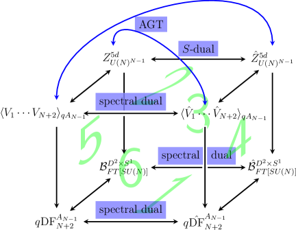
Figure 2: Duality web II incorporates duality web I (face 1 of the cube) in a more general context of $3d$-$5d$-CFT triality.

In the top left corner we have the $5d$ $\mathcal{N}=1$ linear quiver gauge theory with $(N-1)$ $U(N)$ gauge nodes and $N$ (anti-)fundamental matter hypermultiplets on each end of the quiver. This theory is self-dual under $5d$ spectral duality which relates $U(N)^{M-1}$ to $U(M)^{N-1}$ linear quiver theories compactified on a circle.

This is a duality between two low energy descriptions of the same strongly interacting UV SCFT which can be conveniently understood using brane setup Aharony:1997bh . The details of the maps of the parameters of the two theories are nontrivial and have been recently discussed in Bao:2011rc and Bergman:2013aca . This duality has been studied also in the context of integrability in Mironov:2013xva ; Mironov:2012uh ; Mitev:2014isa ; Isachenkov:2014eya ; Zenkevich:2014lca . The term spectral for this duality comes from this interpretation.

We will be focusing on the $\mathbb{R}^{4}\times S^{1}$ instanton partition function which can be realised using geometric engineering as the refined topological string partition function $Z_{\mathrm{top}}$ associated to the square toric diagram depicted in Fig. 7 a). Then one can immediately understand invariance of the square quiver theory under spectral duality as the fiber-base duality corresponding to the reflection along the diagonal of the diagram.

The instanton or topological string partition functions are actually based on $U(N)$ quivers, so if we are interested in the $SU(N)$ case, we should strip off the $U(1)$ contribution. This procedure is discussed for example in Bergman:2013aca . However, for the purpose of this paper, where we discuss instanton partition functions, we can keep the $U(1)$ parts and work with the duality relating $U(N)^{M-1}$ to $U(M)^{N-1}$ theories.

In the other two vertices of face 2 we have an $(N+2)$-point correlator in the the $q$-deformed $A_{N-1}$ Toda theory and its spectral dual.

The $q$-Toda correlators also enjoy the spectral duality relating $(K+2)$-point correlators in $A_{N-1}$ $q$-Toda to $(N+2)$-point correlators in $A_{K-1}$ $q$-Toda theory Zenkevich:2014lca ; Morozov:2015xya which is the avatar of the $5d$ spectral duality relating $U(N)^{M-1}$ to $U(M)^{N-1}$ $5d$ quivers. The identification between $5d$ instanton partition functions and $q$-Toda correlators is the $5d$ uplift of the AGT correspondence Awata:2010yy ; Awata:2009ur . More precisely, the AGT map corresponds to the diagonal edges (shown in blue in Fig. 2), while the map along the edges of face 2 are from the triality approach Aganagic:2013tta ; Aganagic:2014kja .

The vertical arrows going down from the $5d$ web (face 2) to the $3d$ web (face 1) indicate a tuning procedure where the parameters are fixed to specific discrete values. On the gauge theory side (face 3) this tuning corresponds to the so called Higgsing procedure Gaiotto:2012xa ; Mironov:2009qt ; Kozcaz:2010af ; Dimofte:2010tz ; Dorey:2011pa ; Nieri:2013vba ; Gaiotto:2014ina . By tuning the $5d$ Coulomb branch parameters one can degenerate the $5d$ partition function into the partition function of a coupled $5d$–$3d$ system describing co-dimension two defect coupled to the remaining $5d$ bulk theory. We consider particular tuning of the parameters so that the square $5d$ quiver is Higgsed completely, i.e. it reduces to the $3d$ $FT[SU(N)]$ theory coupled to some free $5d$ hypers. We demonstrate this in Sec. 3. Repeating the Higgsing procedure on the spectral dual side we land on the $3d$ spectral dual $FT[SU(N)]$ theory. We then see that $3d$ (self)-duality for $FT[SU(N)]$ follows via Higgsing from the $5d$ spectral duality for the square quiver.

On the $q$-Toda side (face 6) the tuning procedure corresponds to the tuning of the momenta of the vertex operators to special values (corresponding to fully degenerate vertex operators) and to a given assignment of screening charges (corresponding to conditions on the internal momenta, or Coulomb branch parameters). In this way the $q$-Toda $A_{N-1}$ correlator with $N$ semi-degenerate and two full primary operators reduces to the $q$-DF representation of the conformal block.

This explains our previous statement that the integral blocks ${q{\rm DF}}^{A_{N-1}}_{N+2}$ and $\hat{q{\rm DF}}^{A_{N-1}}_{N+2}$ are related by a degenerate version of spectral duality.

Duality web III

Finally, starting from duality web I in Fig. 1 we can obtain another interesting duality web by taking a suitable limit $q\to 1$ as shown in Fig. 3, where the duality web I corresponds to face 1 of the cube.

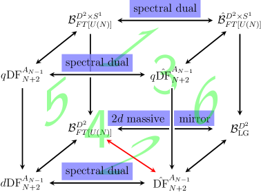
Figure 3: Duality web III. Fig. 1 is the top face (face  1) of the cube. The arrows going downstairs correspond to $q\to 1$ limits. Notice that the two theories related by the spectral duality tend to different theories under $q\to 1$. This asymmetry appears because one needs to choose the scaling of the parameters with $q$ and the spectral duality map relates two different choices.

Let’s consider face 3 in Fig. 3. Here we are performing the reduction of a $3d$ spectral pair of theories on $D_{2}\times S^{1}$ from $3d$ to $2d$ by considering the $q\to 1$ limit, which corresponds to shrinking the $S^{1}$ radius. Taking this limit is subtle, as recently discussed in Aharony:2017adm (and before in Aganagic:2001uw ), since there exist in fact several meaningful limits. Concretely, one can consider the situation when some of the $3d$ real mass parameters are scaled to infinity when going from $3d$ to $2d$ so that $m_{3d}R=m_{2d}$ remains finite as $R\to 0$.

Starting from $\mathcal{B}^{D_{2}\times S^{1}}_{FT[SU(N)]}$ we take the so called Higgs limits which reduces it to the $\mathcal{N}=(2,2)$ gauged linear sigma-model (GLSM) $\mathcal{B}^{D_{2}}_{FT[SU(N)]}$. In the Higgs limit the real mass scaled to infinity is the FI parameter, while the matter remains light, hence the name. This limit generally reduces a $3d$ gauge theory to a $2d$ gauge theory. However, here we want to lift also the Higgs branch and we turn on all the mass deformations so that the $2d$ gauge theory is massive and has $N!$ isolated vacua.

Since spectral duality, similarly to mirror symmetry, swaps Higgs and Coulomb branch parameters, on the dual side the limit has a very different effect. The dual block $\hat{\cal B}^{D_{2}\times S^{1}}_{FT[SU(N)]}$ in the $q\to 1$ limit (which is now a Coulomb limit) reduces to the partition function of a theory of twisted chiral multiplets with twisted Landau-Ginzburg superpotential on $D_{2}$. The horizontal link in face 2 of the cube in Fig. 3 is, therefore, a duality of Hori-Vafa type Hori:2000kt for mass deformed theories.

In general claiming that a duality for mass deformed theories implies a duality for massless theories is dangerous. In particular, in this context the subtleties of inferring a genuine IR $2d$ duality from a duality for $2d$ mass deformed theories obtained from the reduction of pairs of dual theories have been discussed in Aharony:2016jki ; Aharony:2017adm . Here we are not interested in removing the mass deformations since, as we are about to see, the holomorphic blocks for the mass deformed theories can be directly mapped to CFT conformal blocks.

Indeed if we look at face 4 of the duality web III in Fig. 3, we see that we are taking several different $q\to 1$ limits of the $q$-Toda conformal blocks in DF representation. Similarly to the gauge theory side there are several possible ways to take the limit. The limit when we scale the momenta of the vertex operators and keep the insertion points fixed is natural from the CFT point of view and reduces $q$-Toda conformal blocks to conformal blocks of the undeformed Toda CFT. This is exactly the limit we take when we reduce the spectral dual block $q\hat{{\rm DF}}^{A_{N-1}}_{N+2}$ down to the undeformed conformal block $\hat{{\rm DF}}^{A_{N-1}}_{N+2}$ in $2d$ Toda theory. Therefore, we have just discovered that the $2d$ $FT[SU(N)]$ GLSM holomorphic block $\mathcal{B}^{D_{2}}_{FT[SU(N)]}$ is mapped to a $2d$ CFT conformal block $\hat{{\rm DF}}^{A_{N-1}}_{N+2}$ (red diagonal on the face 4). In other terms we have derived the familiar gauge/CFT correspondence between $S^{2}$ partition functions and degenerate CFT correlators discussed in Gomis:2014eya ; Gomis:2016ljm ; Doroud:2012xw as a limit of our $3d$ spectral duality web.

Finally to complete the picture we study what is the effect of the $q\to 1$ limit on the $q{\rm DF}^{A_{N-1}}_{N+2}$ conformal block. This is a less familiar limit which reduces the $q{\rm DF}^{A_{N-1}}_{N+2}$ to a block in the channel with the vertex operators of certain bosonized algebra, which we denote by $d$-$W_{N}$, where $d$ stands for difference in the same way as $q$ in $q$-$W_{N}$ is for quantum. The algebra $d$-$W_{N}$ is a particular limit of the $q$-$W_{N}$ algebra when $q\to 1$. We briefly describe the algebra, correlators and screening charges, leaving a more detailed investigation for the future vertex:future .

The Duality web III is discussed in Sec. 4.

2 Duality web I: $3d$ $FT[SU(N)]$ and $q$-Toda blocks

In this section we study Duality web I shown in Fig. 1. We first introduce the $3d$ holomorphic block ${\cal B}^{D_{2}\times S^{1}}_{T[SU(N)]}(\vec{\mu},\vec{\tau},q,t)$, then we show the effect of adding the flipping fields and discuss the mirror and spectral duals of the theory. Finally we introduce the DF representation for the $q$-Toda blocks and determine the gauge/$q$-DF dual to ${\cal B}^{D_{2}\times S^{1}}_{FT[SU(N)]}(\vec{\mu},\vec{\tau},q,t)$.

2.1 $3d$ blocks for $T[SU(N)]$, flipping fields, mirror and spectral duals

2.1.1 $3d$ holomorphic blocks

We begin by introducing our main character ${\cal B}^{D_{2}\times S^{1}}_{T[SU(N)]}(\vec{\mu},\vec{\tau},q,t)$, the $D_{2}\times S^{1}$ partition function, or $3d$ holomorphic block integral for the $T[SU(N)]$ theory. The $\mathcal{N}=4$ $T[SU(N)]$ theory is a quiver theory with gauge group $U(1)\times U(2)\times\cdots\times U(N-1)$, with bifundamental hypers connecting the $U(N_{a})$ and $U(N_{a+1})$ nodes for $a=1,\cdots,N-2$ and $N$ hypermultiplets at the final node. As an example we present the quiver diagram of the $T[SU(4)]$ theory on Fig. 4.

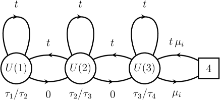
Figure 4: $3d$ $T[SU(4)]$ gauge theory. $\tau_{a}$ are the FI parameters. The masses of the chirals are indicated over or under the corresponding arrows.

We turn on real masses $M^{3d}_{a}$ in the Cartan of the $SU(N)_{H}$ symmetry rotating the Higgs branch and $T^{3d}_{a}$ in the Cartan of the $SU(N)_{C}$ symmetry rotating the Coulomb branch. We also turn on an extra real axial mass deformation $m^{3d}$ for $U(1)_{A}$, the anti-diagonal combination of $U(1)_{C}\times U(1)_{H}\in SU(2)_{C}\times SU(2)_{H}$, which breaks the super-symmetry down to ${\cal N}=2^{*}$. We define the dimensionless mass parameters $M^{\prime}_{a}=RM^{3d}_{a}$, $T^{\prime}_{a}=RT^{3d}_{a}$ and $m^{\prime}=Rm^{3d}$ and the parameter $q=e^{\hbar}=e^{R\epsilon}$, where $R$ is the $S^{1}$ circle radius and $\epsilon$ is the equivariant parameter rotating the cigar $D_{2}$ (see footnote ${}^{\ref{fn:1}}$).

The holomorphic block integral for this theory can be constructed as explained in Beem:2012mb and reads:

$${\cal B}^{D_{2}\times S^{1}}_{T[SU(N)]}(\vec{\mu},\vec{\tau},q,t)=F(q,t,\vec{\tau})\int_{\Gamma}\prod\limits_{a=1}^{N-1}\prod\limits_{i=1}^{a}\left(\frac{dx_{i}^{(a)}}{x_{i}^{(a)}}e^{X_{i}^{(a)}\left(T_{a}-T_{a+1}\right)/\hbar}\,t^{-X_{i}^{(a)}/\hbar}\right)\times\\ \prod\limits_{a=1}^{N-1}\frac{\prod\limits_{i\neq j}^{a}\Big{(}\frac{x^{(a)}_{j}}{x^{(a)}_{i}};q\Big{)}_{\infty}}{\prod\limits_{i,j=1}^{a}\Big{(}t\frac{x^{(a)}_{j}}{x^{(a)}_{i}};q\Big{)}_{\infty}}\prod\limits_{a=1}^{N-2}\prod\limits_{i=1}^{a}\prod\limits_{j=1}^{a+1}\frac{\Big{(}t\frac{x^{(a+1)}_{j}}{x^{(a)}_{i}};q\Big{)}_{\infty}}{\Big{(}\frac{x^{(a+1)}_{j}}{x^{(a)}_{i}};q\Big{)}_{\infty}}\,\prod\limits_{p=1}^{N}\prod\limits_{i=1}^{N-1}\frac{\Big{(}t\frac{\mu_{p}}{x^{(N-1)}_{i}};q\Big{)}_{\infty}}{\Big{(}\frac{\mu_{p}}{x^{(N-1)}_{i}};q\Big{)}_{\infty}}\,,$$ (1)

where the prefactor $F(q,t,\vec{\tau})$ is given by

$$F(q,t,\vec{\tau})=e^{-\frac{2}{3}N(N-1)(2N-1)\hbar\beta(1-\beta)}e^{-\frac{m^{\prime 2}N}{4\hbar}}e^{(1-\beta)\sum_{a=1}^{N-1}\frac{a^{2}}{2}(T_{a+1}-T_{a})}\,.$$ (2)

The integral is performed over the Cartan of the gauge group. For each gauge node we have the contribution of vector and adjoint chiral multiplets (first factor in the second line) given by a ratio of $q$-Pochhammer symbols defined as

$$(x;\,q)_{\infty}=\prod\limits_{k=0}^{\infty}\left(1-xq^{k}\right)\,.$$ (3)

The other factors in the second line are the contributions of the bifundamental chirals and of the fundamentals attached to the last node.

More precisely $(qx^{-1};q)_{\infty}$ is the contribution to the block integral of a chiral multiplet of zero $r$-charge and charge $+1$ under a flavor symmetry with associated real mass $x$, plus a $-\frac{1}{2}$ Chern-Simons unit. This corresponds to a chiral multiplet with Dirichlet boundary conditions along $\partial(D_{2}\times S^{1})=T^{2}$ in Yoshida:2014ssa . A chiral multiplet of $r$-charge $+2$, charge $-1$ and $\frac{1}{2}$ Chern-Simons unit contributes as $(x;q)^{-1}_{\infty}$ and corresponds to Neumann boundary conditions.

If we assemble the matter contribution to the block integrals taking some chirals with Dirichlet and some with Neumann boundary conditions we induce mixed Chern-Simons couplings (because of the attached $\frac{1}{2}$ units) which we might need to compensate by adding extra Chern-Simons terms to the action. With our symmetric choice of boundary conditions the induced dynamical Chern-Simons couplings vanishes automatically, the induced mixed gauge-flavor couplings (the $t^{\frac{-X^{(a)}_{i}}{\hbar}}$ factor in the integrand (1)) renormalize the FI parameters, while the background mixed couplings contribute as the prefactor $F(q,t,\vec{\tau})$.

To present the block in a form more convenient for the following we have shifted the integration variables and identified a new set of exponentiated mass parameters

$$x^{(a)}_{i}=e^{X^{(a)}_{i}},\quad\mu_{p}=e^{M_{p}}=e^{M^{\prime}_{p}}\left(\frac{q}{t}\right)^{N/2},$$

$$\quad\tau_{p}=e^{T_{p}}=e^{T^{\prime}_{p}}t^{N/2},\quad t=q^{\beta}=-q^{1/2}e^{-m^{\prime}}.$$ (9)

An alternative procedure to write down the block integrand $\Upsilon$ is to view it as “square root” of the integrand of the partition function on a compact manifold. Details of this procedure are presented in the Appendix A. This construction also indicates that the contribution of (mixed) Chern-Simons coupling to the partition function should actually be expressed in terms of ratios of theta functions rather than exponents

$$e^{\frac{AB}{\hbar}}\leadsto\frac{\theta_{q}(e^{A})\theta_{q}(e^{B})}{\theta_{q}(e^{A+B})(q;q)_{\infty}}\,$$ (10)

as we discuss in Appendix A. However, for the purpose of this paper we can avoid introducing theta functions and work with the exponents provided that on the integration contours on which we are going to evaluate the blocks, the theta functions and the exponents have no poles and contribute with the same residue. One can check that for $T[SU(N)]$ blocks (1) this will indeed be the case. As will be shown below, the residues of the integrals (1) come in geometric progressions, i.e. a pole $x_{*}$ is accompanied by a string of poles at $q^{k}x_{*}$ with $k\in\mathbb{Z}_{\geq 0}$. Notice then that both sides of Eq. (10) transform in the same way under the $\hbar$-shifts of $A$ and $B$ variables, i.e. under $q$-shifts of $e^{A}$ and $e^{B}$. Thus, their contributions to the residues in the string differ only by an overall constant factor, independent of $k$. This overall constant can be factored out of the integral and included in the normalization factors.

Finally we need to discuss the integration contour on which we evaluate the block integral. The integration in Eq. (1) is performed over a basis of integration contours $\Gamma=\Gamma_{\alpha}$, with $\alpha=1,\ldots,N!$ which are in one to one correspondence with the SUSY vacua, the critical points of the one-loop twisted superpotential $\mathcal{W}^{\mathbb{R}^{2}\times S^{1}}$. The label of the integration contour $\alpha$ is essentially an element of the permutation group $\mathfrak{S}_{N}$. One can understand the origin of the contours $\Gamma_{\alpha}$ as follows.

The integrations in Eq. (1) can be done step by step starting from $x_{i}^{(N-1)}$ and proceeding to $x_{1}^{(1)}$. There are $(N-1)$ integration variables at the first step. The poles of the integrand in $x_{i}^{(N-1)}$ correspond to zeroes of $\prod_{p=1}^{N}\prod_{i=1}^{N-1}(\mu_{p}/x^{(N-1)}_{i};q)_{\infty}$. Moreover, upon closer examination one can see that each $x_{i}^{(N-1)}$ should be of the form $q^{k_{i}^{(N-1)}}\mu_{p}$ with integer $k_{i}^{(N-1)}$ and distinct values of $p$, i.e. each of $(N-1)$ variables $x_{i}^{(N-1)}$ settles at a pole close to its own mass $\mu_{p}$ and no two of the variables can sit near the same mass. Therefore, there are $N$ possible configurations with $(N-1)$ variables filling $N$ places (the integrand is symmetric in $x_{i}^{(N-1)}$). Evaluating the residues in $x_{i}^{(N-1)}$ we can proceed to the next step of integration. Here the situation is repeated: there are $(N-2)$ integration variables $x_{i}^{(N-2)}$ and $(N-1)$ variables $x_{i}^{(N-1)}$ from the previous step play the role of $\mu_{p}$ for them. The poles in $x_{i}^{(N-2)}$ are located at $q^{k_{i}^{(N-2)}-k_{i}^{(N-1)}}x_{j}^{(N-1)}$ with integer $k_{i}^{(N-2)}\geq k_{i}^{(N-1)}$ and again no two variables $x_{i}^{(N-2)}$ can sit near the same $x_{j}^{(N-1)}$. There are $(N-1)$ possibilities at this step. Proceeding further, one notices the general pattern: the poles at each step sit near the poles of the previous step with one free place. Equivalently, there are $(N-1)$ strings of poles with lengths $1$, $2$, …, $(N-1)$, in each of which the poles are close together, e.g. for a string of length $a$ we get

$$x^{(a)}_{a}=q^{k_{a}^{(a)}-k_{a}^{(a+1)}}x^{(a+1)}_{a}=q^{k_{a}^{(a)}-k_{a}^{(a+2)}}x^{(a+2)}_{a}=\ldots=q^{k_{a}^{(a)}-k_{a}^{(N-1)}}x^{(N-1)}_{a}=q^{k_{a}^{(a)}}\mu_{p}$$ (11)

where $k^{(a)}_{i}$ are all integers and we have used the symmetry of the integrand in $x_{1}^{(a)}$, …, $x_{a}^{(a)}$ to set all the lower indices in the string to $a$. Each string terminates at the the free place, not filled by the pole on the next step. Choosing the integration contour is equivalent to specifying which string (of length $a$) sits near which mass $\mu_{p}$. Evidently, any choice can be obtained from a given one by the unique permutaiton of masses $\mu_{p}$. There are therefore $N!$ choices in total, each one corresponding to an element of the symmetric group $\mathfrak{S}_{N}$.

We will do the calculations for a certain convenient reference choice of contour $\alpha=\alpha_{0}$, i.e. in the reference vacuum in which

$$x_{i}^{(a)}=q^{k_{i}^{(a)}}\mu_{i}\qquad\text{(in vacuum $\alpha_{0}$).}$$ (12)

In this vacuum one can expand the vortex partition function as a double series in $\frac{\mu_{i}}{\mu_{i+1}}$ and $\frac{\tau_{i}}{\tau_{i+1}}$, i.e. it is implicitly assumed that the theory sits in the chamber of the moduli space where $\frac{\tau_{i}}{\tau_{i+1}}\ll 1$. Blocks for other vacua can be obtained from the block in the reference vacuum by analytic continuation in $\frac{\tau_{i}}{\tau_{i+1}}$, taking into account the intricate (theta-function) connection coefficients. Let us also notice that since the block is self-dual under mirror symmetry, analytic continuation in $\mu_{i}$ and $\tau_{i}$ will give the same results.

The integration over $\Gamma_{\alpha_{0}}$ yields

$${\cal B}^{D_{2}\times S^{1},\,(\alpha_{0})}_{T[SU(N)]}=Z^{3d,\,(\alpha_{0})}_{\textrm{cl}}Z^{3d,\,(\alpha_{0})}_{1\mathrm{-loop}}Z^{3d,\,(\alpha_{0})}_{\mathrm{vort}}$$ (13)

where $Z^{3d,\,(\alpha_{0})}_{\textrm{cl}}$, $Z^{3d,\,(\alpha_{0})}_{1\mathrm{-loop}}$ and $Z^{3d,\,(\alpha_{0})}_{\mathrm{vort}}$ denote the classical, perturbative one-loop and nonperturbative vortex contributions respectively. We have

$$Z^{3d,\,(\alpha_{0})}_{\textrm{cl}}(\vec{\mu},\vec{\tau},q,t)=F(q,t,\vec{\tau})\,(q;q)_{\infty}^{-\frac{N(N-1)}{2}}\prod_{i=1}^{N}e^{\frac{(T_{i}-T_{N})M_{i}}{\hbar}}t^{-\frac{(N-i)M_{i}}{\hbar}}\prod_{i<j}^{N}\frac{\theta_{q}\left(t\frac{\mu_{j}}{\mu_{i}}\right)}{\theta_{q}\left(\frac{\mu_{j}}{\mu_{i}}\right)}.$$ (14)

The one-loop factor is given by:

$$Z_{1-\mathrm{loop}}^{3d,\,(\alpha_{0})}(\vec{\mu},\vec{\tau},q,t)=\prod_{i<j}\frac{\left(q\frac{\mu_{i}}{\mu_{j}};q\right)_{\infty}}{\left(\frac{q}{t}\frac{\mu_{i}}{\mu_{j}};q\right)_{\infty}}.$$ (15)

Notice that there are cancellations between the theta-functions in classical part and the $q$-Pochhammer functions in the one-loop part. The vortex part reads

$$Z_{\mathrm{vort}}^{3d,\,(\alpha_{0})}(\vec{\mu},\vec{\tau},q,t)=\\ =\sum_{k^{(a)}_{i}\in(\ref{eq:411s})}\prod_{a=1}^{N-1}\left[\left(t\frac{\tau_{a}}{\tau_{a+1}}\right)^{\sum_{i=1}^{a}k^{(a)}_{i}}\prod_{i\neq j}^{a}\frac{\left(t\frac{\mu_{i}}{\mu_{j}};q\right)_{k^{(a)}_{i}-k^{(a)}_{j}}}{\left(\frac{\mu_{i}}{\mu_{j}};q\right)_{k^{(a)}_{i}-k^{(a)}_{j}}}\prod_{i=1}^{a}\prod_{j=1}^{a+1}\frac{\left(\frac{q}{t}\frac{\mu_{i}}{\mu_{j}};q\right)_{k_{i}^{(a)}-k_{j}^{(a+1)}}}{\left(q\frac{\mu_{i}}{\mu_{j}};q\right)_{k_{i}^{(a)}-k_{j}^{(a+1)}}}\right]$$ (16)

where we assume $k^{(N)}_{i}=0$ and the sum is over sets of integers $k_{i}^{(a)}$ satisfying the inequalities

$$\begin{array}[]{ccccc}k^{(1)}_{1}\geq&k^{(2)}_{1}\geq&k^{(3)}_{1}\geq&\cdots\geq&k^{(N-1)}_{1}\geq 0\\ &k^{(2)}_{2}\geq&k^{(3)}_{2}\geq&\cdots\geq&k^{(N-1)}_{2}\geq 0\\ &&k^{(3)}_{3}\geq&\cdots\geq&k^{(N-1)}_{3}\geq 0\\ &&&\ddots&\vdots\\ &&&&k^{(N-1)}_{N-1}\geq 0\\ \end{array}$$ (17)

The block can actually be expressed through higher $q$-hypergeometric functions. This representation also allows one to deduce the monodromy properties of the block under the permutation of parameters $\tau_{i}\to\tau_{\sigma(i)}$. However, these issues will not be considered in the present work. In the semiclassical limit ${\cal B}^{D_{2}\times S^{1},\,(\alpha)}_{T[SU(N)]}\sim e^{\mathcal{W}^{\mathbb{R}^{2}\times S^{1}}_{(\alpha)}/\hbar}$ where $\mathcal{W}^{\mathbb{R}^{2}\times S^{1}}_{(\alpha)}$ is the one-loop twisted superpotential evaluated on the $\alpha$-th vacuum.

2.1.2 Mirror duality

We will consider two similar but subtly different dualities of the $T[SU(N)]$ theory: the mirror duality and the spectral duality, explaining the relationship between them and their differences.

The mirror duality Intriligator:1996ex (which in this case is a self-duality Gaiotto:2008ak ) swaps the Higgs and Coulomb branches and consequently the vector masses and FI parameters $M_{i}\leftrightarrow T_{i}$ and sends $m\leftrightarrow-m$ or in terms of the exponentiated parameters:

$$\mu_{i}\leftrightarrow\tau_{i}\,,\quad t\to\frac{q}{t}\,.$$ (18)

The mirror block is given by:

$$\check{\cal B}^{D_{2}\times S^{1},\,(\alpha)}_{T[SU(N)]}(\vec{\mu},\vec{\tau},q,t)=\mathcal{B}^{D_{2}\times S^{1},\,(\alpha)}_{T[SU(N)]}\left(\vec{\tau},\vec{\mu},q,\frac{q}{t}\right)=\\ =\check{F}(q,t,\vec{\tau})\int_{\Gamma_{\alpha}}\prod\limits_{a=1}^{N-1}\prod\limits_{i=1}^{a}\frac{dx_{i}^{(a)}}{x_{i}^{(a)}}\prod\limits_{a=1}^{N-1}\prod\limits_{i=1}^{a}e^{X_{i}^{(a)}\left(M_{a}-M_{a+1}\right)/\hbar}\left(\frac{t}{q}\right)^{X_{j}^{(a)}/\hbar}\,\times\\ \times\prod\limits_{a=1}^{N-1}\frac{\prod\limits_{i\neq j}^{a}\Big{(}\frac{x^{(a)}_{j}}{x^{(a)}_{i}};q\Big{)}_{\infty}}{\prod\limits_{i,j=1}^{a}\Big{(}\tfrac{q}{t}\frac{x^{(a)}_{j}}{x^{(a)}_{i}};q\Big{)}_{\infty}}\prod\limits_{a=1}^{N-2}\prod\limits_{i=1}^{a}\prod\limits_{j=1}^{a+1}\frac{\Big{(}\tfrac{q}{t}\frac{x^{(a+1)}_{j}}{x^{(a)}_{i}};q\Big{)}_{\infty}}{\Big{(}\frac{x^{(a+1)}_{j}}{x^{(a)}_{i}};q\Big{)}_{\infty}}\,\prod\limits_{p=1}^{N}\prod\limits_{i=1}^{N-1}\frac{\Big{(}\tfrac{q}{t}\frac{\tau_{p}}{x^{(N-1)}_{i}};q\Big{)}_{\infty}}{\Big{(}\frac{\tau_{p}}{x^{(N-1)}_{i}};q\Big{)}_{\infty}}\,.$$ (19)

Showing that the $T[SU(N)]$ holomorphic block is self-dual, i.e. that

$${\cal B}^{D_{2}\times S^{1},\,(\alpha)}_{T[SU(N)]}(\vec{\mu},\vec{\tau},q,t)=\check{\cal B}^{D_{2}\times S^{1},\,(\alpha^{\prime})}_{T[SU(N)]}(\vec{\mu},\vec{\tau},q,t)$$ (20)

or equivalently

$${\cal B}^{D_{2}\times S^{1},\,(\alpha)}_{T[SU(N)]}(\vec{\mu},\vec{\tau},q,t)=\mathcal{B}^{D_{2}\times S^{1},\,(\alpha^{\prime})}_{T[SU(N)]}\left(\vec{\tau},\vec{\mu},q,\frac{q}{t}\right)$$ (21)

is fairly complicated. As discussed in Beem:2012mb if we want to describe how the bases of contours $\alpha$ and $\alpha^{\prime}$ are related we need to take into account Stokes phenomena. One approach is to use mirror-invariant combinations of blocks, e.g. squashed sphere partition functions.

Here we take a different approach showing that the space of blocks is invariant under the mirror map. Following Bullimore:2014awa we can view the space of blocks for the $T[SU(N)]$ theory as the space of solutions to a system of linear difference equations:

$$H_{r}(\mu_{i},q^{\mu_{i}\partial_{\mu_{i}}},q,t){\cal B}^{D_{2}\times S^{1},\,(\alpha)}_{T[SU(N)]}(\vec{\mu},\vec{\tau},q,t)=e_{r}(\vec{\tau}){\cal B}^{D_{2}\times S^{1},\,(\alpha)}_{T[SU(N)]}(\vec{\mu},\vec{\tau},q,t)$$ (22)

where the difference operators are quantum Ruijsenaars-Schneider Hamiltonians Ruijsenaars:1986vq ; Ruijsenaars:1986pp :

$$H_{r}=t^{\frac{r(r-1)}{2}}\sum_{\begin{smallmatrix}I\subset\{1,\ldots,N\}\\ |I|=r\end{smallmatrix}}\prod_{\begin{smallmatrix}i\in I\\ j\notin I\end{smallmatrix}}\frac{t\mu_{i}-\mu_{j}}{\mu_{i}-\mu_{j}}q^{\sum_{i\in I}\mu_{i}\partial_{\mu_{i}}}$$ (23)

and the eigenvalues $e_{r}(\vec{\tau})$ are elementary symmetric polynomials

$$e_{r}(\vec{\tau})=\sum_{i_{1}<\cdots<i_{r}}^{N}\tau_{i_{1}}\cdots\tau_{i_{r}}.\qquad$$ (24)

We give a short proof of Eq. (22) for $r=1$ in Appendix D.1. From the theory of integrable systems it is known that Ruijsenaars-Schneider system has a peculiar duality symmetry called $p$-$q$ duality. It implies that for certain choice of normalization the eigenfunctions of the Ruijsenaars-Schneider Hamiltonian are actually also eigenfunctions of the dual Ruijsenaars-Schneider Hamiltonian. The dual operator is obtained by the mirror map: $\vec{\tau}$ and $\vec{\mu}$ are exchanged as are $t$ and $\frac{q}{t}$. We therefore have:

$$H_{r}\left(\tau_{i},q^{\tau_{i}\partial_{\tau_{i}}},q,\frac{q}{t}\right){\cal B}^{D_{2}\times S^{1},\,(\alpha)}_{T[SU(N)]}(\vec{\mu},\vec{\tau},q,t)=e_{r}(\vec{\mu}){\cal B}^{D_{2}\times S^{1},\,(\alpha)}_{T[SU(N)]}(\vec{\mu},\vec{\tau},q,t)$$ (25)

We prove the simplest case of Eq. (25) for $r=1$, $N=2$ in Appendix D.2. The self-mirror property of the blocks (21) follows from Eqs. (22) and (25).

Alternatively we can check mirror symmetry by “brute force” computation of the partition function. Using explicit expressions (14), (15) and (16) for the one-loop and vortex parts of the partition function we can see that

$$Z_{1\mathrm{-loop}}^{3d,\,(\alpha_{0})}(\vec{\mu},\vec{\tau},q,t)Z_{\mathrm{vort}}^{3d,\,(\alpha_{0})}(\vec{\mu},\vec{\tau},q,t)=Z_{1\mathrm{-loop}}^{3d,\,(\alpha_{0})}\left(\vec{\tau},\vec{\mu},q,\frac{q}{t}\right)Z_{\mathrm{vort}}^{3d\,(\alpha_{0})}\left(\vec{\tau},\vec{\mu},q,\frac{q}{t}\right)$$ (26)

and using the conditions (8) for the sum of masses and FI parameters (up to the equivalence (10)):

$$Z_{\mathrm{cl}}^{3d,\,(\alpha_{0})}(\vec{\mu},\vec{\tau},q,t)=Z_{\mathrm{cl}}^{3d,\,(\alpha_{0})}\left(\vec{\tau},\vec{\mu},q,\frac{q}{t}\right)\,.$$ (27)

As a very simple test of the mirror symmetry (26) consider two degenerate limits of the $T[SU(N)]$ block:

1. $t=q$. In this case all the terms of the vortex series, except the first one vanish:

   $$Z_{\mathrm{vort}}^{3d,(\alpha_{0})}(\vec{\mu},\vec{\tau},q,q)=1.$$ (28)

   The one-loop factor also simplifies and reads

   $$Z_{1\mathrm{-loop}}^{3d,(\alpha_{0})}(\vec{\mu},\vec{\tau},q,q)=\prod_{i<j}\frac{1}{1-\frac{\mu_{i}}{\mu_{j}}}.$$ (29)

2. $t=1$. In this case the vortex sum factorizes into a product of geometric progressions:

   $$Z_{\mathrm{vort}}^{3d,(\alpha_{0})}(\vec{\mu},\vec{\tau},q,1)=\prod_{i<j}\frac{1}{1-\frac{\tau_{i}}{\tau_{j}}}.$$ (30)

   The one-loop part becomes trivial:

   $$Z_{1\mathrm{-loop}}^{3d,(\alpha_{0})}(\vec{\mu},\vec{\tau},q,1)=1.$$ (31)

Two degenerate cases are mirror dual to each other and one immediately sees that Eq. (26) indeed holds in this limit.

2.1.3 Flipping fields and spectral duality

We now introduce the modification of the $T[SU(N)]$ model, in which we add $N^{2}$ singlets fields, the flipping flieds, transforming in the adjoint of the $SU(N)$ flavor symmetry group. These fields modify the $T[SU(N)]$ superpotential by the extra term

$$\mathcal{W}=F_{ij}Q_{ij},$$ (32)

where $Q_{ij}$ is the meson matrix, built from the bifundamental chirals $q_{i}^{a}$ at the rightmost node of the quiver from Fig. 4:

$$Q_{ij}=\sum_{a=1}^{N-1}q_{i}^{a}\bar{q}_{j}^{a},$$ (33)

so that if the bifundamental has $R$-charge $r$, then $R[Q_{ij}]=2r$ and $R[F_{ij}]=2-2r$ . We call the resulting theory $FT[SU(N)]$, where $F$ indicates the flipping of the Higgs branch operators (the meson).

Since flipping fields are gauge singlets, they simply modify the $D_{2}\times S^{1}$ partition function of $T[SU(N)]$ by multiplicative factors in front of the integral:

$${\cal B}^{D_{2}\times S^{1},\,(\alpha)}_{FT[SU(N)]}(\vec{\mu},\vec{\tau},q,t)=f(\vec{\mu},q,t)^{-1}{\cal B}^{D_{2}\times S^{1},\,(\alpha)}_{T[SU(N)]}(\vec{\mu},\vec{\tau},q,t),$$ (34)

where

$$f(\vec{\mu},q,t)=e^{(1-2\beta)\sum_{i=1}^{N}(i-1)M_{i}}\prod_{k<l}^{N}\frac{\left(t\frac{\mu_{k}}{\mu_{l}};q\right)_{\infty}}{\left(\frac{q}{t}\frac{\mu_{k}}{\mu_{l}};q\right)_{\infty}}.$$ (35)

The factor $f(\vec{\mu},q,t)$ crucially modifies the action of the RS Hamiltonians (23) on the block. One proves by direct computation that

$$H_{r}\left(\mu_{i},q^{\mu_{i}\partial_{\mu_{i}}},q,\frac{q}{t}\right)=f(\vec{\mu},q,t)^{-1}H_{r}(\mu_{i},q^{\mu_{i}\partial_{\mu_{i}}},q,t)f(\vec{\mu},q,t).$$ (36)

Since the block ${\cal B}^{D_{2}\times S^{1},\,(\alpha)}_{T[SU(N)]}$ is the eigenfunction of $H_{r}(\mu_{i},q^{\mu_{i}\partial_{\mu_{i}}},q,t)f(\vec{\mu},q,t)$, the holomorphic blocks of the flipped theory $FT[SU(N)]$ are eigenfunctions of $H_{r}\left(\mu_{i},q^{\mu_{i}\partial_{\mu_{i}}},q,\frac{q}{t}\right)$ with the same eigenvalues. Moreover, since $f(\vec{\mu},q,t)$ does not depend on $\tau$, the flipped block $f(\vec{\mu},q,t)^{-1}{\cal B}^{D_{2}\times S^{1}}_{T[SU(N)]}(\vec{\mu},\vec{\tau},q,t)$ is still an eigenfunction of the dual RS Hamiltonians $H_{r}(\tau_{i},q^{\tau_{i}\partial_{\tau_{i}}},q,\frac{q}{t})$. Hence we conclude that because ${\cal B}^{D_{2}\times S^{1}}_{T[SU(N)]}(\vec{\mu},\vec{\tau},q,t)$ is invariant under the mirror duality (18), the flipped block ${\cal B}^{D_{2}\times S^{1}}_{FT[SU(N)]}(\vec{\mu},\vec{\tau},q,t)$ is invariant under the spectral duality:

$$\mu_{i}\leftrightarrow\tau_{i}\,,\quad t\to t\,.$$ (37)

We denote the spectral dual block by $\hat{\mathcal{B}}^{D_{2}\times S^{1},(\alpha)}_{FT[SU(N)]}(\vec{\mu},\vec{\tau},q,t)$ (notice the hat instead of the tick, which we have used for the mirror block). For our special contour $\alpha_{0}$ we have

$$\hat{\mathcal{B}}^{D_{2}\times S^{1},(\alpha_{0})}_{FT[SU(N)]}(\vec{\mu},\vec{\tau},q,t)=\mathcal{B}^{D_{2}\times S^{1},(\alpha_{0})}_{FT[SU(N)]}(\vec{\tau},\vec{\mu},q,t).$$ (38)

We will discuss the origin of the spectral duality when we come to the brane description of the flipped theory in sec. 3. In APZ we will examine in the detail this duality together with another duality obtained from $T[SU(N)]$ by flipping simultaneously the Higgs and Coulomb branch operators.

2.2 $q$-Toda blocks

In a series of works Aganagic:2014kja ; Aganagic:2013tta ; Nedelin:2016gwu partition functions of $3d$ theories have been shown to match conformal blocks in $q$-deformed Toda theories. In this section we will demonstrate the details of the correspondence between holomorphic blocks of the $FT[SU(N)]$ theory and conformal blocks of the $q$-Toda CFT. For this we will first review basic aspects of $A_{n}$ Toda CFT and derive Dotsenko-Fateev (DF) integrals describing conformal blocks in certain channel. In this part we will closely follow Fateev:2007ab ; Aganagic:2014kja ; Aganagic:2013tta . Then we will briefly describe quantum deformation of the Toda theory and corresponding $q\mathrm{DF}$ integrals. Finally we will describe the map between parameters of $FT[SU(N)]$ theory and $q$-Toda CFT that will allow us to manifestly match holomorphic blocks and $q\mathrm{DF}$ integrals on two sides of the correspondence.

2.2.1 Warm-up: conformal block of ordinary Toda

We begin by quickly introducing the integral representation of the Toda conformal blocks, for more detailed review see Fateev:2007ab . The action of the theory is given by

$$S_{\mathrm{Toda}}=\int dz\,d\bar{z}\,\sqrt{g}\left[g^{z\bar{z}}(\partial_{z}\vec{\phi},\partial_{\bar{z}}\vec{\phi})+{\cal Q}_{\beta}(\vec{\rho},\vec{\phi})\,R+\sum\limits_{a=1}^{n}e^{\sqrt{\beta}(\vec{\phi},\,\vec{e}_{(a)})}\right]\,,$$ (39)

where $\vec{\phi}$ is the $(n+1)-$component vector whose components $\phi^{(a)}$ are bososnic fields in $2d$ Toda CFT. $\vec{\rho}$ and $\vec{e}_{(a)}$ are the Weyl vector and the simple roots of the $A_{n}$ Lie algebra respectively:

$$\left(\vec{\rho},\,\vec{\phi}\right)=\frac{1}{2}\sum\limits_{a=1}^{n+1}\left(n-2a+2\right)\phi^{(a)},$$

$$\left(\vec{\phi},\,\vec{e}_{(a)}\right)=\phi^{(a)}-\phi^{(a+1)}.$$ (40)

The first term in the action (39) is just the canonical kinetic term with (inverse) background metric $g^{z\bar{z}}$, while $(.\,,.)$ denote the standard scalar product on ${\mathbb{R}}^{n+1}$. Second term in the action is responsible for the nonminimal coupling of $\vec{\phi}$ to the background curvature $R$. Coefficient of the coupling ${\cal Q}_{\beta}$ is

$${\cal Q}_{\beta}=\sqrt{\beta}-\frac{1}{\sqrt{\beta}}\,,$$ (41)

where $\beta$ is a convenient parameter, which will be used throughout this paper. Finally the last term in (39) is the Toda potential. The theory described above possess $W_{n+1}$ symmetry, which has Virasoro subalgebra with the central charge parametrized by $\beta$ in the following way:

$$c=n-n(n+1)(n+2)\mathcal{Q}_{\beta}^{2}\,.$$ (42)

Basic ingredients we will need for finding correlators in Toda CFT are screening currents

$$S_{(a)}(x)=\,\mathopen{:}\,\exp\left[\sqrt{\beta}\sum\limits_{k\neq 0}\sum\limits_{b=1}^{n+1}\frac{1}{k}c_{k}^{(b)}\,e_{b}^{(a)}\,x^{-k}\right]\,\mathclose{:}\,\exp\left[\sqrt{\beta}\sum\limits_{b=1}^{n+1}Q^{(b)}e_{b}^{(a)}\right]\,x^{\sqrt{\beta}\sum\limits_{b=1}^{n+1}e_{b}^{(a)}P^{(b)}}=\\ =\,\mathopen{:}\,\exp\left[\sqrt{\beta}\sum\limits_{k\neq 0}\left(c_{k}^{(a)}-c_{k}^{(a+1)}\right)\frac{x^{-k}}{k}\right]\,\mathclose{:}\,e^{\sqrt{\beta}\left(Q^{(a)}-Q^{(a+1)}\right)}\,x^{\sqrt{\beta}\left(P^{(a)}-P^{(a+1)}\right)},$$ (43)

where the index $a$, which we call the sector number, runs from $1$ to $n$ for $A_{n}$ theory. We will also need vertex operators defined as follows:

$$V_{\vec{\alpha}}(z)=\,\mathopen{:}\,\exp\left[\frac{1}{\sqrt{\beta}}\sum\limits_{k\neq 0}\sum\limits_{a=1}^{n+1}c_{k}^{(a)}\,\alpha_{a}\,\frac{z^{-k}}{k}\right]\,\mathclose{:}\,e^{\frac{1}{\sqrt{\beta}}\sum\limits_{a=1}^{n+1}Q^{(a)}\alpha_{a}}\,z^{\frac{1}{\sqrt{\beta}}\sum\limits_{a=1}^{n+1}\alpha_{a}P^{(a)}},$$ (44)

where $\vec{\alpha}$ is the $(n+1)-$component weight of the operator. Bosonic operators $c_{k}^{(a)}$ satisfy the Heisenberg algebra

$$[c_{k}^{(a)},c_{m}^{(b)}]=k\,\delta_{k+m,0}\,\delta_{a,b}\,,$$ (45)

and $P^{(a)},\,Q^{(a)}$ are zero-modes satisfying usual commutation relations:

$$\left[P^{(a)},Q^{(b)}\right]=\delta_{a,b}\,.$$ (46)

Now assume that we would like to calculate the following chiral half of the correlator of $(l+2)$ primary vertex operators in Toda theory

$$\langle V_{\vec{\alpha}^{(\infty)}}(\infty)\, V_{\vec{\alpha}^{(1)}}\left(z_{1}\right)\cdots V_{\vec{\alpha}^{(l)}}\left(z_{l}\right)\,V_{\vec{\alpha^{(0)}}}(0)\,\rangle_{\mathrm{Toda}}\,=$$ (47)

$$\int D\vec{\phi}~{}V_{\vec{\alpha}^{(\infty)}}\left(\infty\right)\,V_{\vec{\alpha}^{(1)}}\left(z_{1}\right)\cdots V_{\vec{\alpha}^{(l)}}\left(z_{l}\right)\,V_{\vec{\alpha}^{(0)}}\left(0\right)\,e^{-S_{\mathrm{Toda}}}\,,$$

where $z_{k}$ and $\vec{\alpha}^{(k)}$ are positions and weights of corresponding vertex operator insertions. In general, due to the complicated interaction potential, evaluation of this correlator is extremely hard. However, one can treat Toda potential perturbatively. In this case the full answer for the correlator can be written as the sum of the following correlators in the theory of $(n+1)$ free bosons:

$$\mathrm{DF}_{l+2}^{A_{n}}(z_{1},\ldots,z_{l},\vec{\alpha}^{(0)},\vec{\alpha}^{(1)},\ldots,\vec{\alpha}^{(l)},\vec{N},\beta)\stackrel{{\scriptstyle\mathrm{def}}}{{=}}\langle\vec{\alpha}^{(\infty)}|\,V_{\vec{\alpha}^{(1)}}\left(z_{1}\right)\dots V_{\vec{\alpha}^{(l)}}\left(z_{l}\right)\,\prod_{a=1}^{n}Q_{(a)}^{N_{a}}|\vec{\alpha}^{(0)}\rangle_{\mathrm{free}}\,,$$ (48)

which play the role of the conformal blocks in Toda theory and are usually referred to as Dotsenko-Fateev $\left(\mathrm{DF}\right)$ integrals Dotsenko:1984nm . Here $Q_{(a)}$ are screening charges defined as the integrals of the corresponding screening currents:

$$Q_{(a)}\stackrel{{\scriptstyle\mathrm{def}}}{{=}}\oint dx\,S_{(a)}\left(x\right),$$ (49)

and the states $|\vec{\alpha}^{(0)}\rangle$ and $|\vec{\alpha}^{(\infty)}\rangle$ are defined as follows:

$$|\vec{\alpha}\rangle=\frac{1}{\sqrt{\beta}}e^{\sum\limits_{a=1}^{n+1}\alpha_{a}\,Q^{(a)}}|0\rangle$$ (50)

so that it is the eigenstate of the momentum operators $P^{(a)}$ and is annihilated by the positive modes:

$$P^{(a)}|\vec{\alpha}\rangle=\frac{1}{\sqrt{\beta}}\alpha_{a}|\vec{\alpha}\rangle,$$ (51)

$$c^{(a)}_{n}|\alpha\rangle=0,\qquad\forall n>0.$$ (52)

Due to the operator-state correspondence the ket state $|\vec{\alpha}\rangle$ can be created by the insertion of the vertex operator (44) of weight $\vec{\alpha}$ at point $z=0$. Bra state $\langle\vec{\alpha}|$ is created by inserting the corresponding operator at $z=\infty$. We understand the weight $\vec{\alpha}^{(0)}$ of the vertex operator at zero to be a free parameter of the correlator. Then the weight $\vec{\alpha}^{(\infty)}$ is determined uniquely by the momentum conservation relation, which needs to be satisfied in order for the correlator (48) to be nonzero:

$$2\sqrt{\beta}{\cal Q}_{\beta}\vec{\rho}=\vec{\alpha}^{(0)}+\vec{\alpha}^{(\infty)}+\sum\limits_{j=1}^{l}\vec{\alpha}^{(j)}+\beta\sum\limits_{a=1}^{n}N_{a}\vec{e}_{(a)}\,,$$ (53)

where $\vec{\rho}$ and $\vec{e}_{(k)}$ are given by Eqs. (40). The calculation of the free field correlator (48) is presented in Appendix B.1 and results in

$${\rm DF}^{A_{n}}_{l+2}(z_{1},\ldots,z_{l},\vec{\alpha}^{(0)},\vec{\alpha}^{(1)},\ldots,\vec{\alpha}^{(l)},\vec{N},\beta)\sim\\ \sim\prod\limits_{p<k}^{l}\left(z_{p}-z_{k}\right)^{\frac{1}{\beta}\left(\vec{\alpha}^{(p)},\,\vec{\alpha}^{(k)}\right)}\oint\prod\limits_{a=1}^{n}\prod\limits_{i=1}^{N_{a}}dx^{(a)}_{i}\prod\limits_{a=1}^{n}\prod\limits_{i=1}^{N_{a}}\left(x_{i}^{(a)}\right)^{\beta(N_{a}-N_{a+1}-1)+(\alpha_{a}^{(0)}-\alpha_{a+1}^{(0)})}\times\\ \times\prod\limits_{a=1}^{n}\prod\limits_{i\neq j}^{N_{a}}\left(1-\frac{x_{j}^{(a)}}{x_{i}^{(a)}}\right)^{\beta}\prod_{a=1}^{n-1}\prod\limits_{i=1}^{N_{a}}\prod\limits_{j=1}^{N_{a+1}}\left(1-\frac{x_{j}^{(a+1)}}{x_{i}^{(a)}}\right)^{-\beta}\prod\limits_{p=1}^{l}\prod\limits_{a=1}^{n}\prod\limits_{i=1}^{N_{a}}\left(1-\frac{x_{i}^{(a)}}{z_{p}}\right)^{\alpha_{a}^{(p)}-\alpha_{a+1}^{(p)}}.$$ (54)

In the Virasoro $(A_{1})$ case, the free field integrals are of Selberg type and can be calculated. In the higher rank case the situation is much more complicated and it is known how to evaluate the integrals only for special values of the momenta of the vertex operators. As we will see in this paper we are indeed interested in special value of the momenta for which we can calculate the integrals.

2.2.2 $q$-Toda conformal blocks

The $A_{n}$ Toda theory admits a $q$-deformation which is described in detail in Feigin:1995sf ; Shiraishi:1995rp ; Awata:1996dx . Below we will use free boson representation of this deformed algebra in order to derive the corresponding conformal blocks of the $A_{n}$ $q$-Toda CFT. For our calculations we use screening currents and vertex operators from Aganagic:2013tta ; Aganagic:2014kja , which are given by

$$S^{q}_{(a)}(x)=\,\mathopen{:}\,\exp\left(-\sum\limits_{k>0}\frac{1-t^{k}}{1-q^{k}}c_{k}^{(a)}\frac{x^{-k}}{k}+\sum\limits_{k>0}c_{-k}^{(a)}\frac{x^{k}}{k}\right)\times\\ \times\exp\left(\sum\limits_{k>0}\frac{1-t^{k}}{1-q^{k}}v^{k}\,c_{k}^{(a+1)}\frac{x^{-k}}{k}-\sum\limits_{k>0}v^{k}\,c_{-k}^{(a+1)}\frac{x^{k}}{k}\right)\,\mathclose{:}\,\times\\ \times e^{\sqrt{\beta}Q^{(a)}}\,x^{\sqrt{\beta}P^{(a)}}\,e^{-\sqrt{\beta}Q^{(a+1)}}\,x^{-\sqrt{\beta}P^{(a+1)}}\,$$ (55)

where $t=q^{\beta}$ and we have introduced $v=\sqrt{\frac{q}{t}}$. Similarly to the undeformed case the sector index $a$ runs between $1$ and $n$. Bosonic operators $c_{k}^{(a)},\,Q^{(a)},\,P^{(a)}$ satisfy the Heisenberg algebra (45)

$q$-deformed primary vertex operator is chosen to have the form

$$V^{q}_{\vec{\alpha}}\left(z\right)=\,\mathopen{:}\,\exp\left(\sum\limits_{k>0}\sum\limits_{a=1}^{n+1}\frac{q^{k\alpha_{a}}-1}{1-q^{k}}c_{k}^{(a)}v^{-ka}\frac{z^{-k}}{k}+\right.$$

$$\hskip 17.07164pt\left.\sum\limits_{k>0}\sum\limits_{a=1}^{n+1}\frac{\left(q^{-k\alpha_{a}}-v^{2k\left(N-a-1\right)}\right)}{1-t^{k}}c_{-k}^{(a)}v^{ka}\frac{z^{k}}{k}\right)\,\mathclose{:}\,\times\textrm{e}^{\frac{1}{\sqrt{\beta}}\sum\limits_{a=1}^{n+1}\alpha_{a}\,Q^{(a)}}\,z^{\frac{1}{\sqrt{\beta}}\sum\limits_{a=1}^{n+1}\alpha_{a}\,P^{(a)}}\,,$$ (56)

where $\vec{\alpha}$ is the weight vector just as in Eq. (44). Essentially this is the vertex operator of the same form as the one that can be found in Aganagic:2013tta ; Aganagic:2014kja . However in the latter case authors have omitted central part of the operator, i.e. $\vec{\alpha}$-independent part that commutes with the screening current $S(x)$ given in (55). As we will see this part appears to be essential for us so we keep it.

As in the non-deformed case we are interested in the following free field correlator

$$q\mathrm{DF}_{l+2}^{A_{n}}(z_{1},\ldots,z_{l},\vec{\alpha}^{(0)},\vec{\alpha}^{(1)},\ldots,\vec{\alpha}^{(l)},\vec{N},q,t)\stackrel{{\scriptstyle\mathrm{def}}}{{=}}\langle\vec{\alpha}^{(\infty)}|\,V^{q}_{\vec{\alpha}^{(1)}}\left(z_{1}\right)\dots V^{q}_{\vec{\alpha}^{(l)}}\left(z_{l}\right)\,\prod_{a=1}^{n}Q_{(a)}^{N_{a}}|\vec{\alpha}^{(0)}\rangle_{\mathrm{free}}\,,$$ (57)

where $Q_{(a)}$ are screening charges related to the screening currents (55) in the same way as in non-deformed case (49). Initial and final states $|\vec{\alpha}^{(0)}\rangle$, $|\vec{\alpha}^{(\infty)}\rangle$ are defined in Eq. (50). Conservation relation (53) that constraints weights of the vertex operators also holds in the $q$-deformed case.

The free field calculation in the $q$-Toda conformal block is similar to the undeformed case and is presented in Appendix B.2. The final result is given by the following matrix integral:

$$q{\rm DF}^{A_{n}}_{l+2}(z_{1},\ldots,z_{l},\vec{\alpha}^{(0)},\vec{\alpha}^{(1)},\ldots,\vec{\alpha}^{(l)},\vec{N},q,t)\sim C_{{\rm vert}}^{q}\left(\vec{\alpha},z\right)\prod\limits_{p}^{l}z_{p}^{\frac{1}{\beta}\left(\vec{\alpha}^{(p)},\vec{\alpha}^{(0)}\right)+\sum\limits_{a=1}^{N}N_{a}\left(\alpha_{a}^{(p)}-\alpha_{a+1}^{(p)}\right)}\times\\ \oint\prod\limits_{a=1}^{n}\prod\limits_{i=1}^{N_{a}}dx^{(a)}_{i}\prod\limits_{a=1}^{n}\prod\limits_{i=1}^{N_{a}}\left(x_{i}^{(a)}\right)^{\beta(N_{a}-N_{a+1}-1)+(\alpha_{a}^{(0)}-\alpha_{a+1}^{(0)})+\sum\limits_{p=1}^{l}\left(\alpha_{a}^{(p)}-\alpha_{a+1}^{(p)}\right)}\times\\ \times\prod\limits_{a=1}^{n}\prod\limits_{i\neq j}^{N_{a}}\frac{\left(\frac{x_{j}^{(a)}}{x_{i}^{(a)}};q\right)_{\infty}}{\left(t\frac{x_{j}^{(a)}}{x_{i}^{(a)}};q\right)_{\infty}}\prod_{a=1}^{n-1}\prod\limits_{i=1}^{N_{a}}\prod\limits_{j=1}^{N_{a+1}}\frac{\left(u\frac{x_{j}^{(a+1)}}{x_{i}^{(a)}};q\right)_{\infty}}{\left(v\frac{x_{j}^{(a+1)}}{x_{i}^{(a)}};q\right)_{\infty}}\prod_{p=1}^{l}\prod_{a=1}^{n}\prod_{i=1}^{N_{a}}\frac{\left(q^{1-\alpha^{(p)}_{a}}v^{a}\frac{z_{p}}{x_{i}^{(a)}};q\right)_{\infty}}{\left(q^{1-\alpha^{(p)}_{a+1}}v^{a}\frac{z_{p}}{x_{i}^{(a)}};q\right)_{\infty}}\,,$$ (58)

where $u=\sqrt{qt}$ and $C_{{\rm vert}}$ is the prefactor coming from ordering different vertex operators. Precise form of this prefactor is given in (142). The expression appears to be very complicated. However, as we will see further, in cases relevant for us, in particular when some of the vertices are (semi-)degenerate, this expression simplifies drastically.

2.3 Map between $FT[SU(N)]$ and $q$-Toda blocks

The $q$-Toda blocks in DF representation have been shown to map to the holomorphic blocks of the handsaw quiver theory Aganagic:2013tta ; Aganagic:2014kja . Here we are interested in the simpler case of the $FT[SU(N)]$ holomorphic block which can be mapped to a $A_{N-1}$ $q$-Toda block with full primary initial and final states and $N$ fully degenerate primary vertex operators between them (we again omit the prefactors in front of both integrals in holomorphic and conformal blocks):

$${\cal B}^{D_{2}\times S^{1}}_{FT[SU(N)]}\sim q\mathrm{DF}^{A_{N-1}}_{N+2}\,.$$ (59)

with the identification of parameters which we give momentarily.

We begin by considering an $(N+2)-$point conformal block with the weights of the vertex operators satisfying the following relation:

$$\alpha_{a+1}^{(p)}=\alpha_{a}^{(p)},\qquad a=1,\dots,N-2,\quad p=1,\dots,N\,.$$ (60)

The initial state has generic weight $\vec{\alpha}^{(0)}$ and the weight $\vec{\alpha}^{(\infty)}$ is fixed by the charge conservation condition  (53). We also specify the number of screening charges to be $N_{a}=a$ for $a=1,\ldots,N-1$. With this choice of momenta (60) and screening charges $q$-Toda conformal block (58) reduces to the following expression

$$\langle\vec{\alpha}^{(\infty)}|V^{q}_{\vec{\alpha}^{(1)}}(z_{1})\cdots V^{q}_{\vec{\alpha}^{(N)}}(z_{N})\prod\limits_{a=1}^{N-1}\left(Q_{(a)}^{q}\right)^{a}|\vec{\alpha}^{(0)}\rangle\sim\oint\prod\limits_{a=1}^{N-1}\prod\limits_{i=1}^{a}dy^{(a)}_{i}\times\\ \times\prod\limits_{i=1}^{N-1}\left(y_{i}^{(N-1)}\right)^{\beta\left(N-2\right)+\alpha_{N-1}^{(0)}-\alpha_{N}^{(0)}+\sum\limits_{p=1}^{N}\left(\alpha_{N-1}^{(p)}-\alpha_{N}^{(p)}\right)}\prod\limits_{a=1}^{N-2}\prod\limits_{i=1}^{a}\left(y_{i}^{(a)}\right)^{-2\beta+\alpha_{a}^{(0)}-\alpha_{a+1}^{(0)}}\times\\ \times\prod\limits_{a=1}^{N-1}\prod\limits_{i\neq j}^{a}\frac{\left(\frac{y_{j}^{(a)}}{y_{i}^{(a)}};q\right)_{\infty}}{\left(t\frac{y_{j}^{(a)}}{y_{i}^{(a)}};q\right)_{\infty}}\prod_{a=1}^{N-2}\prod\limits_{i=1}^{a}\prod\limits_{j=1}^{a+1}\frac{\left(u\frac{y_{j}^{(a+1)}}{y_{i}^{(a)}};q\right)_{\infty}}{\left(v\frac{y_{j}^{(a+1)}}{y_{i}^{(a)}};q\right)_{\infty}}\prod\limits_{p=1}^{N}\prod\limits_{i=1}^{N-1}\frac{\left(q^{1-\alpha^{(p)}_{N-1}}v^{N-1}\frac{z_{p}}{y_{i}^{(N-1)}};q\right)_{\infty}}{\left(q^{1-\alpha^{(p)}_{N}}v^{N-1}\frac{z_{p}}{y_{i}^{(N-1)}};q\right)_{\infty}}\,,$$ (61)

where we have omitted prefactors coming from the ordering of the vertices to concentrate only on the integral for the moment. Expression on the r.h.s of (61) is almost of the same form as the integral in ${\cal B}^{D_{2}\times S^{1}}_{FT[SU(N)]}$ block  (1). To complete the map we need to impose a further restriction on the $q$-Toda vertex operator parameters. First of all looking on the one-loop contribution of the vector and adjoint multiplets in the block integral (1) we can see that the gauge theory parameter $t$ related to the $3d$ axial mass is identified with the $t$-parameter of Toda CFT deformation. Then in order to match the contribution of the bifundamental hypers with the corresponding term in the correlator (61) we need to make the following identification between the integration variables $y$ in the $q$-DF integral (61) and $x$ in the holomorphic block integral (1):

$$y_{i}^{(a)}=x_{i}^{(a)}v^{-a}.$$ (62)

To identify the last product in the third line of Eq. (61) with the contribution of the fundamental chiral multiplets we need

$$\mu_{p}=q^{1-\alpha_{N}^{(p)}}\,v^{2N-2}z_{p}\,,$$

$$t\mu_{p}=q^{1-\alpha_{N-1}^{(p)}}v^{2N-2}z_{p}\,,$$ (63)

which amounts to requiring

$$\alpha_{N}^{(p)}-\alpha_{N-1}^{(p)}=\beta\,.$$ (64)

Eq. (64) together with the condition (60) completely fixes all the components of the vertex weight vectors in terms of the last components so that all weights have the form

$$\vec{\alpha}^{(p)}=(g_{p}-\beta)\vec{1}+\beta\vec{\omega}_{N-1}\,,$$ (65)

where $g_{p}$ is arbitrary constant and $\vec{\omega}_{N-1}$ is the highest weight vector of $A_{N-1}$. The map (63) give us freedom to choose $g_{p}$ freely. For example we can absorbe it into the definition of the insertion points $z^{\prime}_{p}=q^{\beta-g_{p}}z_{p}$ and consequently have $\mu_{p}=v^{2N}z^{\prime}_{p}$. Alternatively we can simultaneously shift of all the components of the vertex operator weight. This operation does not affect the $q$-DF integral (54) as it only contribute an overall factor in front of the integral which we omit anyway. So we choose to set $g_{p}=\beta$ corresponding to vertices with fully degenerate momenta (corresponding to simple degenerate punctures in the AGT setup):

$$\vec{\alpha}^{(p)}=\beta\vec{\omega}_{N-1}\,.$$ (66)

Finally we need to identify the FI parameters of the $FT[SU(N)]$ theory with the components of the initial and final momenta of $q$-Toda CFT $\alpha_{a}^{(0)}$. This can be done by looking at the powers of $y_{i}^{(a)}$ in the $q$-DF integral (61) and $e^{X_{i}^{(a)}}$ powers in the block integral (1). We arrive at the following relation:

$$\alpha_{a}^{(0)}-\alpha_{a+1}^{(0)}+1-2\beta=\frac{T_{a}-T_{a+1}}{\hbar}-\beta,$$ (67)

and thus

$$T_{a}=\hbar\left(\alpha_{a}^{(0)}+\left(\beta-1\right)a\right).$$ (68)

Summarizing, the dictionary between the ${\cal B}^{D_{2}\times S^{1}}_{FT[SU(N)]}$ block (1) and the $q$-Toda block $q{\rm DF}^{A_{N-1}}_{N+2}\left(z_{1},\ldots,z_{N},\vec{\alpha}^{(0)},\beta\vec{\omega}_{N},\ldots,\beta\vec{\omega}_{N},[1,2,\ldots,N-1],q,q^{\beta}\right)$ is given in Table 1.

${\cal B}^{D_{2}\times S^{1}}_{FT[SU(N)]}$	Identification	$q\mathrm{DF}^{A_{N-1}}_{N+2}$
Integration parameters $x_{i}^{(a)}$	$y_{i}^{(a)}=x_{i}^{(a)}v^{-a}$	Screening current positions $y_{i}^{(a)}$
Axial mass $t$	$t=q^{\beta}$	Central charge parameter $\beta$
Vector masses $\mu_{p}$	$\mu_{p}=v^{2N}z_{p}$	Positions of the vertex operators $z_{p}$
FI parameters $T_{a}$	$T_{a}=\hbar\left(\alpha_{a}^{(0)}+(\beta-1)a\right)$	Initial state momentum vector $\vec{\alpha}^{(0)}$

Table 1: Map between the parameter of the $FT[SU(N)]$ holomorphic block (1) and the conformal block (58) of the $q$-Toda theory.

It is important to notice here that with the choice (66) of the vertex operator weights and the map of parameters specified in Table 1 the prefactor $C_{{\rm vert}}^{q}$ in the $q\mathrm{DF}$ integral (58) simplifies drastically and reduces to:

$$C_{{\rm vert}}^{q}\rightarrow\prod\limits_{p<r}\mu_{p}^{\beta}\frac{\left(\frac{q}{t}\frac{\mu_{r}}{\mu_{p}};q\right)_{\infty}}{\left(t\frac{\mu_{r}}{\mu_{p}};q\right)_{\infty}}\,.$$ (69)

As we can see ratio of $q$-Pochhammers in this expression exactly reproduces contribution (35) of the flipping singlets into holomorphic block of $FT\left[SU(N)\right]$ theory. However we still omit mixed Chern-Simons terms since their matching would require more delicate calculation of conformal blocks.

To complete the discussion of Duality web I in Fig. 1 we need to comment on the counterpart of the $3d$ spectral duality relating the $3d$ holomorphic blocks ${\cal B}^{D_{2}\times S^{1}}_{FT[SU(N)]}$ and $\hat{\cal B}^{D_{2}\times S^{1}}_{FT[SU(N)]}$ by the map (37). In this context the spectral duality reads:

$$\hat{C}~{}q\hat{{\rm DF}}^{A_{N-1}}_{N+2}\left(\hat{z}_{1},\ldots,\hat{z}_{N},\hat{\vec{\alpha}}^{(0)},\hat{\beta}\vec{\omega}_{N},\ldots,\hat{\beta}\vec{\omega}_{N},[1,2,\ldots,N-1],q,q^{\hat{\beta}}\right)=\\ =C~{}q{\rm DF}^{A_{N-1}}_{N+2}\left(z_{1},\ldots,z_{N},\vec{\alpha}^{(0)},\beta\vec{\omega}_{N},\ldots,\beta\vec{\omega}_{N},[1,2,\ldots,N-1],q,q^{\beta}\right)\,.$$ (70)

The parameters of the dual DF integrals are related by the spectral duality map:

$$\hat{\beta}=\beta,$$

$$\hat{\alpha}^{(0)}_{p}=\frac{1}{\hbar}\log z_{p}+(1-\beta)(N+p),$$ (71)

$$\hat{z}_{p}=q^{\alpha_{p}^{(0)}+(N+p)(\beta-1)},$$

which swaps the coordinates of the vertex operators with the momenta. The prefactor $C=C\left(z_{1},\ldots,z_{N},\vec{\alpha}^{(0)},\beta\right)$ (and similarly $\hat{C}$) is given by the product of the omitted factor in front of integral in the $q$-Toda conformal block (58) and $F^{-1}(q,\,t,\,\vec{\tau})$ from the holomorphic block (1).

3 Duality web II: $FT[SU(N)]$ and its spectral dual via Higgsing

In this section we will describe how to obtain the partition function of the $3d$ $\mathcal{N}=2$ $FT[SU(N)]$ gauge theory on $\mathbb{R}^{2}_{q}\times S^{1}$ by Higgsing the $5d$ $\mathcal{N}=1$ square linear quiver theory on the $\Omega$-background $\mathbb{R}^{4}_{q,t}\times S^{1}$.

We consider the $3d$-$5d$ version of the setup of Hanany:2003hp ; Hanany:2004ea ; Dorey:2011pa ; Aganagic:2013tta . Physically the $3d$ theory lives on the worldvolume of the vortices appearing in the Higgs phase of the $5d$ theory. Using a Type IIB brane setup with NS5 and D5 branes to engineer the $5d$ linear quiver theory we can realise the $3d$ vortex theory as the low energy theory on the D3 branes stretched between NS5 and D5 branes. The spectral self-duality of the $FT[SU(N)]$ theory descends from IIB S-duality which swaps NS5 and D5 branes.

3.1 $5d$ instanton partition function, Higgs branch and the vortex theory

Consider the $5d$ $\mathcal{N}=1$ square quiver gauge theory with gauge group $U(N)^{N-1}$ in $\Omega$-background. An example of such theory for $N=4$ is depicted in Fig. 5. The parameters of the theory are:

1. Vacuum expectation values (vevs) of the adjoint scalar fields. We denote the exponentiated vev of the $i$-th diagonal component of the adjoint scalar of the $a$-the gauge group by $a_{i}^{(a)}$, $i=1,\ldots,N$, $a=1,\ldots,N-1$.

2. Couplings $\Lambda_{a}$, $a=1,\ldots,(N-1)$ of the gauge groups.

3. Masses $m_{i}$ (resp. $\bar{m}_{i}$) of the fundamental (resp. antifundamental) hypermultiplets coupled to the first (resp. the last) gauge groups in the linear quiver.

4. Bifundamental masses $m_{\mathrm{bif}}^{(a,a+1)}$. Since we consider the $U(N)$ case these parameters could be eliminated by shifting the ratio of trace parts $\prod_{i=1}^{N}\frac{a^{(a)}_{i}}{a^{(a+1)}_{i}}\to\prod_{i=1}^{N}\frac{a^{(a)}_{i}}{m_{\mathrm{bif}}^{(a,a+1)}a^{(a+1)}_{i}}$. However, we will keep them as separate parameters to make the formulas more symmetric.

5. Parameters $q$ and $t$ of the $\Omega$-deformation.

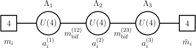
Figure 5: $5d$ linear “square” quiver gauge theory with gauge group $U(4)^{3}$. $a^{(a)}_{i}$ are the exponentiated vevs of the adjoint scalars. $m_{\mathrm{bif}}^{(a,a+1)}$, $m_{i}$, $\bar{m}_{i}$ and $\Lambda^{(a)}$ are the exponentiated masses and gauge couplings.

The $\Omega$-background partition function of the theory is given by (the $5d$ version of) the instanton partition function Nekrasov:2002qd . It is the product of three factors: the classical piece $Z_{\mathrm{cl}}^{5d}$, the one-loop determinant $Z_{1-\mathrm{loop}}^{5d}$ and the instanton part $Z_{\mathrm{inst}}^{5d}$, of which we write down explicitly only the last one:

$$Z_{\mathrm{inst}}^{5d}(a^{(a)}_{i},m_{i},\bar{m}_{i},m_{\mathrm{bif}}^{(a,a+1)},\Lambda_{a})=\sum_{\vec{Y}^{(1)},\ldots,\vec{Y}^{(N-1)}}\prod_{a=1}^{N-1}\Lambda_{a}^{|\vec{Y}^{(a)}|}\times\\ \times z_{\mathrm{fund}}(\vec{m},\vec{a}^{(1)},\vec{Y}^{(1)})\frac{\prod_{a=1}^{N-2}z_{\mathrm{bif}}(m_{\mathrm{bif}}^{(a,a+1)},\vec{a}^{(a+1)},\vec{a}^{(a)},\vec{Y}^{(a+1)},\vec{Y}^{(a)})}{\prod_{a=1}^{N-1}z_{\mathrm{vect}}(\vec{a}^{(a)},\vec{Y}^{(a)})}\,z_{\overline{\mathrm{fund}}}(\vec{\bar{m}},\vec{a}^{(N-1)},\vec{Y}^{(N-1)})$$ (72)

where $\vec{Y}^{(a)}$, $a=1,\ldots,(N-1)$ each denote the $N$-tuple of Young diagrams, $\vec{Y}^{(a)}=\{Y^{(a)}_{1},\ldots,Y^{(a)}_{N}\}$ and

$$z_{\mathrm{fund}}(\vec{m},\vec{a},\vec{Y})=\prod_{r=1}^{N}\prod_{s=1}^{N}\prod_{(i,j)\in Y_{r}}\left(1-\frac{a_{r}}{m_{s}}q^{j-1}t^{1-i}\right),$$ (73)

$$z_{\overline{\mathrm{fund}}}(\vec{m},\vec{a},\vec{Y})=\prod_{r=1}^{N}\prod_{s=1}^{N}\prod_{(i,j)\in Y_{r}}\left(1-\frac{m_{s}}{a_{r}}q^{1-j}t^{i-1}\right),$$ (74)

$$z_{\mathrm{bif}}(m_{\mathrm{bif}},\vec{a},\vec{b},\vec{Y},\vec{W})=\prod_{r=1}^{N}\prod_{s=1}^{N}\prod_{(i,j)\in Y_{r}}\left(1-\frac{a_{r}}{m_{\mathrm{bif}}b_{s}}q^{Y_{r,i}-j}t^{W^{\mathrm{T}}_{s,j}-i+1}\right)\times$$ (75)

$$\times\prod_{(k,l)\in W_{s}}\left(1-\frac{a_{r}}{m_{\mathrm{bif}}b_{s}}q^{-W_{s,i}+j-1}t^{-Y^{\mathrm{T}}_{r,j}+i}\right),$$ (76)

$$z_{\mathrm{vect}}(\vec{a},\vec{Y})=z_{\mathrm{bif}}(1,\vec{a},\vec{a},\vec{Y},\vec{Y}).$$ (77)

We are now going to show how the instanton partition functions can be reduced via Higgsing to the $3d$ vortex partition function for the $FT[SU(N)]$ theory. As mentioned in the Introduction, Higgsing a $5d$ partition function typically produces the partition function of a coupled $5d$-$3d$ system describing a codimension-two surface operator coupled to the bulk theory. Here we are interested in the case where the $5d$ bulk theory is trivial, consisting only of a bunch of decoupled hypermultiplets and so rather than reducing to a coupled system, the Higgsing directly yields the $3d$ vortex theory.

$FT[SU(2)]$ case

Let us start with the simplest example of the square $U(2)$ theory, i.e. the $U(2)$ gauge theory with two fundamental and two antifundamental multiplets. The Higgs branch touches the Coulomb branch at the point $a_{i}=m_{i}$, $i=1,2$. The theory on the Higgs branch contains nonabelian vortex strings with worldvolumes spanning $\mathbb{R}_{q}^{2}\times S^{1}\subset\mathbb{R}^{4}_{q,t}\times S^{1}$. The $3d$ theory on charge $M$ vortices is the $\mathcal{N}=2$ $U(M)$ theory with

• adjoint multiplet with mass $t$,

• two fundamental multiplets with masses $\mu_{i}=m_{i}$,

• two antifundamental multiplets with masses $\bar{\mu}_{i}\frac{q}{t}=\bar{m}_{i}$.

When the 3d FI parameter is turned on the $3d$ theory is on the Higgs branch and the gauge group is broken to $U(M_{1})\times U(M_{2})$ with $M_{1}+M_{2}=M$.

The vortex theory is actually dual to the theory at certain discrete points on the Coulomb branch without any vortices Dorey:2011pa . In particular the $5d$ theory on the Higgs branch with $U(M_{1})\times U(M_{2})$ vortex is equivalent to the theory on the Coulomb branch with

$$a_{i}=m_{i}\,t^{M_{i}},\qquad i=1,2.$$ (78)

Indeed for $a_{i}=m_{i}\,t^{M_{i}}$ the sum over Young tableaux in the instanton partition function $Z_{\mathrm{inst}}^{5d}$ (72) truncates so that only the diagrams $Y_{i}$ of length $l(Y_{i})\leq M_{i}$ contribute. The surviving diagrams correspond to the values of the $3d$ adjoint scalar fields fixed under the localization, which in the IR are diagonal $M_{1}\times M_{1}$ and $M_{2}\times M_{2}$ matrices. The instanton contributions for these diagrams indeed match those of the vortex expansion $Z_{\mathrm{vort}}^{3d}$ of the $3d$ theory Aganagic:2013tta with the following dictionary:

$5d$ square $U(2)$		$3d$ vortex theory
coupling	$\Lambda$	$\tau$	FI parameter
fundamental masses	$m_{i}$	$\mu_{i}$	fundamental masses
antifundamental masses	$\bar{m}_{i}$	$\bar{\mu}_{i}=\frac{q}{t}\bar{m}_{i}$	antifundamental masses
Coulomb parameters	$a_{i}=m_{i}t^{M_{i}}$	$U(M_{1})\times U(M_{2})$	rank of the gauge groups
$\Omega$-parameter	$t$	$t$	adjoint mass
$\Omega$-parameter	$q$	$q$	$\Omega$-parameter

To obtain the $FT[SU(2)]$ vortex partition functions one needs to further tune the parameters of the $3d/5d$ setup choosing $M_{1}=1$ and $M_{2}=0$ and setting the antifundamental masses to $\bar{m}_{i}=\frac{t^{2}}{q}m_{i}$ (consistent with the cubic superpotential of the $\mathcal{N}=2^{*}$ theory).

$FT[SU(N)]$ case

The Higgsing procedure described above can be easily extended to the $FT[SU(N)]$ case which can be obtained from the square $U(N)^{N-1}$ $5d$ by tuning the masses and the Coulomb parameters to the following values:

$$\begin{array}[]{c}a^{(1)}_{1}=m_{1}t,\\ a^{(1)}_{2}=m_{2},\\ a^{(1)}_{3}=m_{3},\\ \vdots\\ a^{(1)}_{N-1}=m_{N-1},\\ a^{(1)}_{N}=m_{N},\end{array}\qquad\begin{array}[]{c}a^{(2)}_{1}=m_{1}t,\\ a^{(2)}_{2}=m_{2}t,\\ a^{(2)}_{3}=m_{3},\\ \vdots\\ a^{(2)}_{N-1}=m_{N-1},\\ a^{(2)}_{N}=m_{N},\end{array}\cdots\qquad\begin{array}[]{c}a^{(N-1)}_{1}=m_{1}t,\\ a^{(N-1)}_{2}=m_{2}t,\\ a^{(N-1)}_{3}=m_{3}t,\\ \vdots\\ a^{(N-1)}_{N-1}=m_{N-1}t,\\ a^{(N-1)}_{N}=m_{N},\end{array}\qquad\begin{array}[]{c}\bar{m}_{1}=m_{1}\frac{t^{2}}{q},\\ \bar{m}_{2}=m_{2}\frac{t^{2}}{q},\\ \bar{m}_{3}=m_{3}\frac{t^{2}}{q},\\ \vdots\\ \bar{m}_{N-1}=m_{N-1}\frac{t^{2}}{q},\\ \bar{m}_{N}=m_{N}\frac{t^{2}}{q},\end{array}$$ (79)

and $m_{\mathrm{bif}}^{(r,r+1)}=1$ for all $r$. After this specialization the instanton sum in (72) over $N$-tuples of Young diagrams $\vec{Y}^{(a)}$ truncates: the only surviving terms are those with $\vec{Y}^{(a)}$ of the following form:

$$\begin{array}[]{c}Y^{(1)}_{1}=[k^{(1)}_{1}],\\ Y^{(1)}_{2}=\varnothing,\\ Y^{(1)}_{3}=\varnothing,\\ \vdots\\ Y^{(1)}_{N-1}=\varnothing,\\ Y^{(1)}_{N}=\varnothing,\end{array}\qquad\begin{array}[]{c}Y^{(2)}_{1}=[k^{(2)}_{1}],\\ Y^{(2)}_{2}=[k^{(2)}_{2}],\\ Y^{(2)}_{3}=\varnothing,\\ \vdots\\ Y^{(2)}_{N-1}=\varnothing,\\ Y^{(2)}_{N}=\varnothing,\end{array}\qquad\cdots\qquad\begin{array}[]{c}Y^{(N-1)}_{1}=[k^{(N-1)}_{1}],\\ Y^{(N-1)}_{2}=[k^{(N-1)}_{2}],\\ Y^{(N-1)}_{3}=[k^{(N-1)}_{3}],\\ \vdots\\ Y^{(N-1)}_{N-1}=[k^{(N-1)}_{N-1}],\\ Y^{(N-1)}_{N}=\varnothing,\end{array}$$ (80)

where the integers $k^{(a)}_{i}$ satisfy the constraints (17). We then see that the instanton partition function reduces exactly to the vortex series (16).

3.2 $(p,q)$-webs, topological strings and the geometric transition

We can realize $3d$ and $5d$ theories in terms of $(p,q)$-brane webs in Type IIB string theory Aharony:1997bh . The $(p,q)$-brane web $\mathfrak{S}$ for the $U(N)^{N-1}$ theory consists of $N$ NS5 branes (vertical) and $N$ D5’ branes (horizontal) as shown in Fig. 6, a). The NS5 and D5’ branes fuse to form $(1,1)$-branes, which are diagonal in Fig. 6. The tensions of the branes are balanced regardless of their relative positions, therefore the system has moduli, corresponding to the parameters of the gauge theory. The $5d$ theory obtained in this way lies on the Coulomb branch, so some of the brane moduli are Coulomb parameters. Others correspond to masses and gauge couplings. Concretely, changing the Coulomb moduli means changing the positions of the internal branes, while fixing the semi-infinite ones.

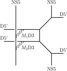
a)	b)

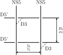
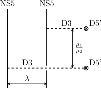
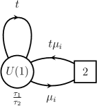
c)	d)	e)

Figure 6: a) $(p,q)$-brane web $\mathfrak{S}$, corresponding to the $5d$ $U(2)$ square gauge theory. The picture can also be viewed as the toric diagram of the CY. Compactifying M-theory on this CY one arrives at the same gauge theory. b) One NS5 brane is separated in the transverse direction, so that the gauge theory goes onto the Higgs branch. The dashed lines denote two stacks of $M_{1}$ and $M_{2}$ D3 branes respectively stretching between the NS5 and D5’ branes. One can also view this picture as describing the CY background after the geometric transition. c) The brane setup corresponding to the $3d$ $FT[SU(2)]$ theory where $M_{1}=1$ and $M_{2}=0$. The masses $\mu_{1,2}$ and FI parameters $\tau_{1,2}$ of the gauge theory are encoded in the positions of the branes as shown. Notice that the second NS5 brane is also detached from the web and a single D3 is stretched between it and the second D5’ brane. This imposes the condition $\bar{\mu}_{i}=t\mu_{i}$. d) Another projection of the brane setup c). The distance between the NS5 branes in the transversal directions $\lambda$ corresponds to the coupling constant of the $3d$ theory which does not enter the holomorphic block. e) The $3d$ $FT[SU(2)]$ gauge theory obtained form the brane setup c), d). The deformation parameter $t$ giving mass to the adjoint multiplet originates from the $\Omega$-background in the $\mathbb{R}^{4}_{q,t}$ part of the $10d$ geometry.

Where is the Higgs branch in the brane setup? The origin of the Higgs branch appears when at least one NS5 brane does not fuse with any of the D5’ branes passing vertically through the whole picture. The NS5 brane can then be separated from the rest of the $(p,q)$-web in the directions perpendicular to the plane of the picture, as shown in Fig. 6, b). The position of the NS5 brane in these directions corresponds to the Higgs branch moduli. The vortex strings appearing in the Higgs phase of the $5d$ theory correspond to the D3 branes stretching between the D5’ branes and the separated NS5 brane. $3d$ $FT[SU(N)]$ theory is obtained by further tuning the positions of the branes as shown in Fig. 6.

Notice that we need also to detach the last NS5 brane from the web and stretch a single D3 between it and one of the D5’ brane. This imposes the condition on the fundamental chiral masses $\bar{\mu}_{i}=t\mu_{i}$. Notice the resulting diagonal pattern of the D3 branes.

To find the matter content of the $3d$ theory on the D3 branes it is instructive to look at a different projection of the brane setup shown in Fig. 6, d). The D3 segment between the two NS5 branes supports $4d$ $U(1)$ theory, which in the IR becomes $3d$, since the length of the segment is finite, while open strings stretching between D3 branes across NS5 branes give rise to bifundamental filelds. The flipping fields arise, because the D3 branes can move along the five-branes in the directions perpendicular to those drawn in Fig. 6.

The distance between the D5’ branes $\frac{\mu_{1}}{\mu_{2}}$ determines the masses of the fundamental multiplets while the distance between the NS5 branes in the “Coulomb” direction $\frac{\tau_{1}}{\tau_{2}}$ gives the FI parameter of the $3d$ $FT[SU(2)]$ gauge theory.

We can now observe that the brane web in Fig. 6, c) under the action of Type IIB $S$-duality which exchanges the NS5 and D5’ branes, thus effectively taking the mirror image along the diagonal, is sent into an identical web diagram with mass and FI parameters exchanged. This is due to two properties.

1. We have $N$ NS5 and $N$ D5’ branes. This is the reason why we call it square theory.

2. The number of D3 branes sitting at each intersection is tuned so that the whole collection is symmetric along the diagonal.

This construction indicates that the $3d$ spectral self-duality of the $FT[SU(N)]$ theory follows from Type IIB $S$-duality.

We can see this very explicitly if we transform our Type IIB $(p,q)$-brane web into a purely geometric background of M-theory without any five-branes (this technique is known as geometric engineering of gauge theories). The background is a toric CY three-fold $\mathfrak{S}$ with toric diagram copied after the $(p,q)$-brane web. One can then compute the partition function of M-theory on $\mathfrak{S}\times\mathbb{R}^{4}_{q,t}\times S^{1}$ by computing the refined (with $(q,t)$-deformation) topological string partition function $Z_{\mathrm{top}}[X]$ Aganagic:2003db ; Iqbal:2007ii .

The positions of the five-branes become complexified Kähler parameters of the CY $\mathfrak{S}$. It will be natural for us to trade the Kähler parameters of the compact two-cycles on CY for the so-called spectral parameters living on the edges of the diagram. They are defined so that for two parallel lines on the diagram with spectral parameters $z$ and $w$ the Kähler parameter of the two-cycle between the lines is given by $\frac{z}{w}$:

(81)

and are conserved at the brane junctions:

(82)

The toric diagram of the CY background $\mathfrak{S}$ corresponding to the $5d$ $U(4)^{3}$ square gauge theory is shown in Fig. 7 (we use the shorthand notation for the resolved conifold pieces of the geometry, as shown in b)). The Higgs branch of the $5d$ gauge theory appears when all the conifold resolutions along one of the vertical lines become degenerate, i.e. their Kähler parameters vanish. In this case the CY can be deformed, so that each crossing looks like a deformed conifold geometry, locally a $T^{*}S^{3}$. Resolved and deformed backgrounds of (refined) topological strings are related by the geometric transition Gopakumar:1998ki ; Aganagic:2012hs , i.e. at quantized values of the conifold Kähler parameter $Q=\sqrt{\frac{q}{t}}t^{N}$ the resolution is equivalent to the deformed geometry with a stack of $N$ Lagrangian branes wrapped over the compact three-cycle. The background after the geometric transition can be illustrated by Fig. 6 b) and c) with dashed lines now playing the role of Lagrangian branes. Quantized values of the Kähler parameters correspond to the points (78) on the Coulomb branch of the $5d$ gauge theory, while the deformed geometry with Lagrangian branes corresponds to $5d$ theory on the Higgs branch with a collection of vortices, on which the $3d$ $FT[SU(N)]$ theory leaves. We call the Higgsed version of CY $\mathfrak{S}$ by $\mathcal{S}$ (so that $\mathcal{S}$ represents a particular point in the Kähler moduli space of $\mathfrak{S}$). In this way, geometric transition explains the Higgsing procedure described above.

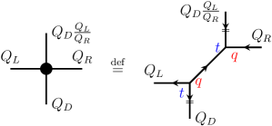
a)	b)

Figure 7: a) The toric diagram $\mathfrak{S}$ producing the square gauge theory from Fig. 5. The labels of the lines correspond to the spectral parameters on the toric diagram and encode the parameters of the gauge theory. b) The shorthand notation for the crossings: black circles denote the resolved conifold geometries with general Kähler parameters. Notice that the spectral parameter on the upper vertical leg is determined by the “conservation law”.

a)	b)

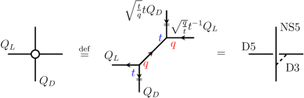
c)

Figure 8: a) The toric diagram $\mathcal{S}$ for the higgsed gauge theory, i.e. for parameters tuned as in Eq. (79). We have rotated the picture compared to Fig. 6 by $\frac{\pi}{2}$ to aid explicit refined topological string computations. b) The “empty crossing” denotes the fully degenerate refined conifold amplitude. c) The “higgsed crossing” denote refined conifold amplitude corresponding to the geometric transition of the deformed geometry with a single brane wrapping $S^{3}$.

We can then calculate the closed topological string partition $Z_{\mathrm{top}}(\vec{\mu},\vec{\tau},q,t)$ for the CY background $\mathcal{S}$ with tuned Kähler paramters in Fig. 8 using the refined topological vertex Aganagic:2003db ; Iqbal:2007ii or using the techniques of Awata:2016riz ; Mironov:2016yue and check that it reproduces the vortex plus one loop factor of the holomorphic block ${\cal B}^{D_{2}\times S^{1}}_{FT[SU(N)]}(\vec{\mu},\vec{\tau},q,t)$:

$$\prod_{i<j}\frac{\left(\frac{q}{t}\frac{\mu_{i}}{\mu_{j}};q\right)_{\infty}}{\left(t\frac{\mu_{i}}{\mu_{j}};q\right)_{\infty}}Z_{1\mathrm{-loop}}^{3d,\,(\alpha_{0})}(\vec{\mu},\vec{\tau},q,t)Z_{\mathrm{vort}}^{3d,\,(\alpha_{0})}(\vec{\mu},\vec{\tau},q,t)=Z_{\mathrm{top}}(\vec{\mu},\vec{\tau},q,t)$$ (83)

where we have omitted an overall constant independent of $\vec{\mu}$ and $\vec{\tau}$ in $Z_{\mathrm{top}}$. The first factor in the l.h.s. of Eq. (83) is the contribution of the flipping fields (it is essentially $f(\vec{\mu},q,t)^{-1}$ up to a power factor).

Notice how the two sides of Eq. (83) behave in the unrefined limit $t=q$. The topological string partition function for $t=q$ simplifies, and in particular empty crossings become really non-interacting, so that the whole diagram in Fig. 8 a) splits into a product of non-interacting resolved conifold pieces, so that $Z_{\mathrm{top}}(\vec{\mu},\vec{\tau},q,q)=1$. This agrees with the behavior of the one-loop and vortex partition functions we have observed in Eqs. (28), (29).

3.3 Fiber-base and spectral duality

Finally we discuss how the spectral self-duality of the $FT[SU(N)]$ holomorphic block appears from the geometric engineering perspective. The CY background $\mathcal{S}$ in Fig. 8 is invariant under the action of the fiber-base duality (reflection along the diagonal) which swaps fiber and base Kähler parameters or, equivalently, exchanges $\mu_{i}$ with $\tau_{i}$. So is the corresponding refined topological string partition function which satisfies:

$$Z_{\mathrm{top}}(\vec{\mu},\vec{\tau},q,t)=Z_{\mathrm{top}}(\vec{\tau},\vec{\mu},q,t)\,.$$ (84)

Notice that the parameters $q$ and $t$ of the refined topological string are left invariant by the action of the fiber-base duality.

Considering the Higgsing relation (83) we see that Eq. (84) implies

$$\prod_{i<j}\frac{\left(\frac{q}{t}\frac{\mu_{i}}{\mu_{j}};q\right)_{\infty}}{\left(t\frac{\mu_{i}}{\mu_{j}};q\right)_{\infty}}Z_{1\mathrm{-loop}}^{3d,\,(\alpha_{0})}(\vec{\mu},\vec{\tau},q,t)Z_{\mathrm{vort}}^{3d,\,(\alpha_{0})}(\vec{\mu},\vec{\tau},q,t)=\\ =\prod_{i<j}\frac{\left(\frac{q}{t}\frac{\tau_{i}}{\tau_{j}};q\right)_{\infty}}{\left(t\frac{\tau_{i}}{\tau_{j}};q\right)_{\infty}}Z_{1\mathrm{-loop}}^{3d,\,(\alpha_{0})}(\vec{\tau},\vec{\mu},q,t)Z_{\mathrm{vort}}^{3d,\,(\alpha_{0})}(\vec{\tau},\vec{\mu},q,t)\,.$$ (85)

We can then easily check that the contact terms in $f(\vec{\mu},q,t)$ satisfy the following relation

$$e^{-(1-2\beta)\sum_{i=1}^{N}(i-1)M_{i}}Z^{3d,\,(\alpha_{0})}_{\textrm{cl}}(\vec{\mu},\vec{\tau},q,t)=e^{-(1-2\beta)\sum_{i=1}^{N}(i-1)T_{i}}Z^{3d,\,(\alpha_{0})}_{\textrm{cl}}(\vec{\tau},\vec{\mu},q,t).$$ (86)

Hence we conclude that

$${\cal B}^{D_{2}\times S^{1}}_{FT[SU(N)]}\left(\vec{\tau},\vec{\mu},q,t\right)=\prod_{i<j}\frac{\left(\frac{q}{t}\frac{\mu_{i}}{\mu_{j}};q\right)_{\infty}}{\left(t\frac{\mu_{i}}{\mu_{j}};q\right)_{\infty}}Z_{1\mathrm{-loop}}^{3d,\,(\alpha_{0})}(\vec{\mu},\vec{\tau},q,t)Z_{\mathrm{vort}}^{3d,\,(\alpha_{0})}(\vec{\mu},\vec{\tau},q,t)=\\ =\prod_{i<j}\frac{\left(\frac{q}{t}\frac{\tau_{i}}{\tau_{j}};q\right)_{\infty}}{\left(t\frac{\tau_{i}}{\tau_{j}};q\right)_{\infty}}Z_{1\mathrm{-loop}}^{3d,\,(\alpha_{0})}(\vec{\tau},\vec{\mu},q,t)Z_{\mathrm{vort}}^{3d,\,(\alpha_{0})}(\vec{\tau},\vec{\mu},q,t)={\cal B}^{D_{2}\times S^{1}}_{FT[SU(N)]}\left(\vec{\mu},\vec{\tau},q,t\right)$$ (87)

This is one of our main results: we have an explicit realization of how the $3d$ spectral duality relation (37) follows from the fiber-base self-duality of the CY background $\mathcal{S}$.

We will provide more examples of this idea in APZ .

3.3.1 Symmetries of the blocks: the Ding-Iohara-Miki algebra approach

In this section we briefly discuss the algebraic version of the topological vertex formalism Awata:2011ce based on the representation theory of Ding-Iohara-Miki (DIM) algebra $U_{q,t}(\widehat{\widehat{\mathfrak{gl}}}_{1})$ 1996q.alg…..8002D ; doi:10.1063/1.2823979 . This algebra is a central extension and quantum deformation of the algebra of double loops in $\mathbb{C}$, i.e. of the polynomials $x^{n}y^{m}$, $n,m\in\mathbb{Z}$. The deformation parameters $q$ and $t$ correspond to the parameters of the $\Omega$-background in the $5d$ gauge theory, or to the parameters of the $\mathcal{N}=2$ deformation of the $3d$ $\mathcal{N}=4$ $T[SU(N)]$ theory. The algebra is symmetric under any permutation of the triplet of parameters $(q,t^{-1},\frac{t}{q})$. However, the representations retain only part of this symmetry. The simplest representation is the representation on the Fock space $\mathcal{F}$ with convenient choice of basis given by Macdonald polynomials $M_{Y}^{(q,t)}(a_{-n})|\mathrm{vac}\rangle$. It (along with its tensor powers) corresponds to the action of the algebra on the equivariant cohomology of instanton moduli space of the $5d$ gauge theory. The representation is invariant under the exchange of $q$ and $t^{-1}$, provided one maps the creation operators $a_{-n}$ into $-\frac{1-q^{n}}{1-t^{n}}a_{-n}$. In particular, in the basis of Macdonald polynomials the symmetry corresponds to the transposition of the Young diagram $Y$:

$$M_{Y^{\mathrm{T}}}^{(t^{-1},q^{-1})}(a_{-n})|\mathrm{vac}\rangle=M_{Y}^{(q,t)}\left(-\frac{1-q^{n}}{1-t^{n}}a_{-n}\right)|\mathrm{vac}\rangle$$ (88)

From physical point of view this symmetry is natural, since $q$ and $t^{-1}$ are two equivariant parameters acting along two orthogonal planes in the $\mathbb{R}^{4}_{q,t}$.

In the algebraic construction of refined topological strings each leg of the brane web corresponds to a Fock representation. The direction of the leg corresponds to vector of two central charges $(k_{1},k_{2})$ of the DIM algebra. Thus we call Fock representations vertical or horizontal depending on the value of the central charges. Brane junction corresponds to DIM algebra intertwining operator acting from the tensor product of two Fock spaces (e.g. vertical and horizontal) into a single Fock space (e.g. diagonal) or vice versa. Gluing of vertices corresponds to the composition of intertwiners. Spectral duality of the brane web corresponds to the Miki automorphism of the DIM algebra, which in particular takes the mirror image of the central charge vector $(k_{1},k_{2})\mapsto(k_{2},-k_{1})$. Mirror image of charge vectors implies mirror image of all the brane web. Miki automorphism does not change $q$ and $t$ parameters. Thus, we conclude that partition function of refined topological string corresponding to the brane web in Fig. 8, a) is invariant under the symmetry (84).

When composing two intertwiners (or gluing two vertices in the brane web) we need to perform the sum over intermediate states belonging to the Fock representation, i.e. over all Young diagrams $Y$. However, for the specific choice of spectral parameters corresponding to the higgsed theory, only a subset of diagrams yields nonzero matrix elements. In the setup shown in Fig. 8. Those are diagrams with at most one column, i.e. $Y=[k]$. The sum over these diagrams corresponds to the sum over $k_{i}^{(a)}$ in the vortex partition function (16). The subspace of the Fock representation $\mathcal{F}$ retains larger symmetry of the original DIM algebra. In particular it turns out that, besides the standard $q\leftrightarrow t^{-1}$ symmetry, the symmetry $t\leftrightarrow\frac{q}{t}$ is also secretly preserved in the partition function. A simple example of such situation occurs in the basis of Macdonald polynomials. The polynomials corresponding to totally antisymmetric reps do not depend on $q$ and $t$, so they do not feel the exchange of $t$ and $\frac{q}{t}$. We plan to return to this point in the future.

4 Duality web III

In this section we study the Duality web III depicted in Fig. 3.

4.1 $2d$ GLSM, Hori-Vafa dual and Toda blocks

On the gauge theory side (face 3) we consider the limit where we shrink the $S^{1}$ circle and reduce the $FT[SU(N)]$ theory from $D_{2}\times S^{1}$ to the cigar $D_{2}$. This corresponds to taking $q=e^{\hbar}\to 1$ since $\hbar=R\epsilon$ where $R$ is the circle radius and $\epsilon$ is the equivariant parameter rotating the cigar which we keep fixed (and indeed can set its numerical value to one).

As we have already mentioned in the Introduction there are various ways to take the $2d$ limit, here we consider the limit which is the ordinary dimensional reduction of the $3d$ $FT[SU(N)]$ theory down to the theory with the same matter content in $2d$. This limit is called the Higgs limit in Aharony:2017adm ; Aganagic:2001uw , since the $3d$ FI parameters are large and lift the Coulomb branch while the matter fields remain light.

In our conventions (where the $3d$ real mass parameters are dimensionless as they have already been rescaled by $R$), this limit is implemented by taking $T_{a}$ finite as $\hbar\to 0$ and

$$\mu_{j}=e^{M_{j}}\equiv e^{\hbar f_{j}}=q^{f_{j}},\quad t=q^{\beta}\,.$$ (89)

We identify $f_{j}$ and $\beta$ as the (dimensionless) twisted mass parameters for the $SU(N)\times U(1)_{A}$ symmetries. We will keep all these deformations finite to ensure that the theory has N isolated massive vacua.

When we take the limit on the partition functions we also have to consider possible rescaling of the integration variable which can single out the contribution for vacua located at infinite distances. In the Higgs limit case the vacua remain at finite distances which corresponds to taking:

$$x^{(a)}_{i}=e^{X^{(a)}_{i}}=e^{\hbar w^{(a)}_{i}}=q^{w^{(a)}_{i}}\,.$$ (90)

With this parameterisation, using the following limit discussed in the Appendix C

$$\lim\limits_{q\to 1}\frac{(q^{x};q)_{\infty}}{(q;q)_{\infty}}=\left(-\hbar\right)^{1-x}\frac{1}{\Gamma(x)}\,,$$ (91)

we can take the $q\to 1$ limit of the block ${\cal B}^{D_{2}\times S^{1}}_{\mathrm{FT[SU(N)]}}$ and find:

$$\lim_{q\to 1}{\cal B}^{D_{2}\times S^{1}}_{\mathrm{FT[SU(N)]}}=\hbar^{\frac{N(N-1)(\beta-1)}{2}}(-1)^{\frac{1}{2}N(N-1)\beta}\prod\limits_{a=1}^{N-1}e^{(1-\beta)a^{2}\left(T_{a+1}-T_{a}\right)}\prod_{k<l}^{N}\frac{\Gamma(f_{k}-f_{l}+\beta)}{\Gamma(f_{k}-f_{l}+1-\beta)}\times\\ \int\prod\limits_{a=1}^{N-1}\prod\limits_{i=1}^{a}dw_{i}^{(a)}\prod\limits_{a=1}^{N-1}\prod\limits_{i=1}^{a}e^{w_{i}^{(a)}\left(T_{a}-T_{a+1}\right)}\prod\limits_{a=1}^{N-1}\frac{\prod\limits_{i,j}^{a}\Gamma\left(\beta+w_{i}^{(a)}-w_{j}^{(a)}\right)}{\prod\limits_{i\neq j}^{a}\Gamma\left(w_{i}^{(a)}-w_{j}^{(a)}\right)}\,\times\\ \times\prod\limits_{a=1}^{N-2}\prod\limits_{i=1}^{a}\prod\limits_{j=1}^{a+1}\frac{\Gamma\left(w_{j}^{(a+1)}-w_{i}^{(a)}\right)}{\Gamma\left(\beta+w_{j}^{(a+1)}-w_{i}^{(a)}\right)}\,\prod\limits_{p=1}^{N}\prod\limits_{i=1}^{N-1}\frac{\Gamma\left(f_{p}-w_{i}^{(N-1)}\right)}{\Gamma\left(\beta+f_{p}-w_{i}^{(N-1)}\right)}=\\ \sim\hbar^{\frac{N(N-1)(\beta-1)}{2}}{\cal B}^{D_{2}}_{\mathrm{FT[SU(N)]}}\,.$$ (92)

The divergent $\hbar$ prefactor in the above expressions is the leading contribution to the saddle point and we will have to match it to analogue divergence arising from the limit of the dual block. Then we identified up to a contact term the $D_{2}$ partition functions ${\cal B}^{D_{2}}_{\mathrm{FT[SU(N)]}}$ of the ${\cal N}=(2,2)$ $FT[SU(N)]$ theory which can be written down following Hori:2013ika ; Honda:2013uca . The chiral multiplets contributions to the partition function are now given by Gamma functions which sit in the numerator or in the denominator depending whether they correspond to Neumann or Dirichlet boundary conditions as in the $3d$ case. Our symmetric choice of the boundary condition for the chiral multiplets corresponds to a particular boundary condition.

On the spectral dual side, where the FI and mass parameters are swapped the limit we have just described acts very differently and it corresponds to the so called Coulomb limit. Indeed now the chirals are massive and the Higgs branch is lifted. As before however we keep all the deformations parameters non zero so that the $2d$ theory still has isolated vacua. This time however the vacua are at infinity. In our convention this means that the $3d$ Coulomb brach parameters $x^{(a)}_{i}=e^{X^{(a)}_{i}}$ stay finite as $\hbar\to 0$.

In this case we will use the following property of $q$-Pochhammer symbols

$$\lim\limits_{q\to 1}\frac{(q^{a}x;q)_{\infty}}{(q^{b}x;q)_{\infty}}=(1-x)^{b-a}\,,$$ (93)

which is proven in the Appendix C and find that:

$$\lim_{q\to 1}\hat{\cal B}^{D_{2}\times S^{1}}_{FT[SU(N)]}=(-\hbar)^{\frac{N(N-1)}{2}(\beta-1)}\Gamma(\beta)^{\frac{N(N-1)}{2}}e^{(2\beta-1)\sum_{a=1}^{N}(a-1)T_{a}}\prod_{k<l}^{N}(1-\tfrac{\tau_{k}}{\tau_{l}})^{{2\beta-1}}\times\\ \times\int\prod\limits_{a=1}^{N-1}\prod\limits_{i=1}^{a}\frac{dx^{(a)}_{i}}{x_{i}^{(a)}}\prod\limits_{a=1}^{N-1}\prod\limits_{i=1}^{a}\left(x_{i}^{(a)}\right)^{f^{(a)}-f^{(a+1)}-\beta}\prod\limits_{a=1}^{N-1}\prod\limits_{i\neq j}^{a}\left(1-\frac{x_{j}^{(a)}}{x_{i}^{(a)}}\right)^{\beta}\times\\ \times\prod_{a=1}^{N-2}\prod\limits_{i=1}^{a}\prod\limits_{j=1}^{a+1}\left(1-\frac{x_{j}^{(a+1)}}{x_{i}^{(a)}}\right)^{-\beta}\prod\limits_{p=1}^{N}\prod\limits_{i=1}^{N-1}\left(1-\frac{\tau_{p}}{x_{i}^{(N-1)}}\right)^{-\beta}\sim\\ \sim\hbar^{\frac{N(N-1)(\beta-1)}{2}}\hat{DF}^{A_{N-1}}_{N+2}\,.$$ (94)

We notice first of all that the divergent prefactor in the above expression matches the one we found by taking the limit on the spectral dual side, which guarantees that we are comparing the right set of vacua on both sides of the duality.

In the last equality we identified the integral block $\hat{\mathrm{DF}}^{A_{N-1}}_{N+2}$ of $\left(N+2\right)$ vertex operators in $A_{N-1}$ Toda CFT with screening charges $N_{a}=a$ and the following identification of parameters:

$$\hat{\vec{\alpha}}^{(p)}=\beta\vec{\omega}_{N-1}\,,\quad\hat{\alpha}_{a}^{(0)}=f^{(a)}+(1-\beta)a\,,\quad\hat{z}_{p}=\tau_{p}\,,\quad\hat{\beta}=\beta\,.$$ (95)

As before we put $\sim$ in (94) because we omitted the overall $z_{p}$ dependent factor in the Toda conformal block (54).

Thus we have obtained the red diagonal link in the web 3 which relates the $2d$ gauge theory to the CFT block. Notice that the map (95) between the parameters of the gauge theory and Toda block is consistent with the $\hbar\to 0$ limit of the previously derived gauge/CFT correspondence map (see Table 1) after the spectral duality transformation $\tau_{p}\leftrightarrow\mu_{p}$, $\beta\rightarrow\beta$.

To make contact with the Hori-Vafa dual theory of twisted chiral multiplets which we expect to find on the bottom right corner of face 3 in Fig. 3 we simply need to exponentiate the integrand $\mathcal{I}$ in eq. (94) as $\mathcal{I}=\exp(\log\mathcal{I})$ and identify $\log(\mathcal{I})$ with $\mathcal{W}$ the twisted superpotential contribution to the $D_{2}$ partition function of the Hori-Vafa dual theory. The dual theory also has $N(N-1)/2$ un-gauged chiral multiplets which yield the $\Gamma(\beta)$ factors.

Notice that we keep all the FI and the twisted mass deformations on. This is necessary for the convergence of the integrals (and to relate them to CFT) so the match of the $D_{2}$ partition functions is a check of the duality for the mass deformed theories with isolated vacua. As recently discussed in Aharony:2016jki ; Aharony:2017adm it is quite subtle to understand what happens when these deformations are lifted and generically we are not guaranteed to find a proper IR duality for massless theories.

4.2 $2d$ GLSM and the $d$-Virasoro algebra

Finally the remaining corner of face 2, labelled $d$DF${}^{A_{N-1}}_{N+2}$ is to be interpreted as a conformal block of an unconventional limit of the $q$-$W_{N}$ algebra. Here we briefly sketch the construction of this theory restricting ourselves to the case $N=2$. We then start from the $q$-Virasoro algebra which is generated by the current $T(z)$ satisfying the quadratic relation:

$$f\left(\frac{w}{z}\right)T(z)T(w)-f\left(\frac{z}{w}\right)T(w)T(z)=-\frac{(1-q)(1-t^{-1})}{1-\frac{q}{t}}\left(\delta_{\times}\left(\frac{q}{t}\frac{w}{z}\right)-\delta_{\times}\left(\frac{t}{q}\frac{w}{z}\right)\right)$$ (96)

where

$$f(x)=\exp\left[\sum_{n\geq 1}\frac{(1-q^{n})(1-t^{-n})}{1+\left(\frac{q}{t}\right)^{n}}\frac{x^{n}}{n}\right]=\frac{\left(qx;\frac{q^{2}}{t^{2}}\right)_{\infty}\left(t^{-1}x;\frac{q^{2}}{t^{2}}\right)_{\infty}}{(1-x)\left(\frac{q^{2}}{t}x;\frac{q^{2}}{t^{2}}\right)_{\infty}\left(\frac{q}{t^{2}}x;\frac{q^{2}}{t^{2}}\right)_{\infty}}$$ (97)

and $\delta_{\times}(x)=\sum_{n\in\mathbb{Z}}x^{n}$ is the multiplicative delta-function. One can understand $\delta_{\times}(x)$ as the delta function on the unit circle, where $x=e^{i\phi}$, since

$$\sum_{n\in\mathbb{Z}}e^{in\phi}=\sum_{m\in\mathbb{Z}}\delta_{+}(\phi-2\pi m),$$

and $\delta_{+}(u)$ is the standard (additive) Dirac delta delta-function.

The $q$-Virasoro algebra in the familiar limit $q=e^{\hbar}\to 1$ and $t=q^{\beta}$ with fixed $\beta$ reduces to the Virasoro algebra. This can be seen by taking the above limit in eq. (96) keeping fixed also the positions of the currents $z$ and $w$. In this case one recovers the quadratic relation for the ordinary Virasoro algebra. The current $T(z)$ also reduces to the Virasoro current $L(z)$:

$$T(z)=2+\beta\hbar^{2}\left(z^{2}L(z)+\frac{1}{4}\left(\sqrt{\beta}-\frac{1}{\sqrt{\beta}}\right)^{2}\right)+\ldots$$ (98)

We can also take an unconventional limit of the quadratic relation (96) where positions $z$ and $w$ scale as powers of $q$:

$$z=q^{u},\qquad w=q^{v},$$ (99)

and the current $t(u)=\lim_{q\to 1}T(q^{u})$ remains finite then the relations of the algebra become

$$g(v-u)t(u)t(v)-g(u-v)t(v)t(u)=-\frac{\beta}{1-\beta}\left(\delta_{+}(v-u+1-\beta)-\delta_{+}(v-u-1+\beta)\right)$$ (100)

where the structure function becomes

$$g(u)=\frac{2(1-\beta)}{u}\frac{\Gamma\left(\frac{u+2-\beta}{2(1-\beta)}\right)\Gamma\left(\frac{u+1-2\beta}{2(1-\beta)}\right)}{\Gamma\left(\frac{u+1}{2(1-\beta)}\right)\Gamma\left(\frac{u-\beta}{2(1-\beta)}\right)}.$$ (101)

The main effect of the limit is that the $q$-Pochhammer symbols in the definition of the $q$-Virasoro structure function (97) turn into Euler gamma functions. Essentially this algebra, which we will call $d$-Virasoro algebra, is the additive analogue of the $q$-Virasoro algebra.

We claim that conformal blocks of the $d$-Virasoro algebra have the DF representation which coincides with the GLSM localization integrals. Moreover, these blocks are spectral dual to the ordinary CFT conformal blocks, so that the positions of the vertex operators in $d$-Virasoro become momenta in the dual CFT and vice versa.

The algebra (100) can be bosonized as follows. We express the current as:

$$t(u)=\Lambda_{1}(u)+\Lambda_{2}(u),$$ (102)

where

$$\Lambda_{1}(u)=e^{\tilde{Q}}\left(g(u)\right)^{\tilde{P}}\,\mathopen{:}\,\exp\Bigl{[}\sum_{n\geq 1}\frac{1}{n}c_{-n}\left(u^{n}-(u-\beta)^{n}\right)-\\ -\sum_{k\geq 0}\sum_{n\geq 1}\frac{1}{n}c_{n}(-1)^{k}\left((u-(1-\beta)k)^{-n}-(u-1-(1-\beta)k)^{-n}\right)\Bigr{]}\,\mathclose{:}\,,$$ (103)

$$\Lambda_{2}(u)=e^{-\tilde{Q}}\left(g(u)\right)^{-\tilde{P}}\,\mathopen{:}\,\exp\Bigl{[}-\sum_{n\geq 1}\frac{1}{n}c_{-n}\left((u+\beta-1)^{n}-(u-1)^{n}\right)+\\ +\sum_{k\geq 0}\sum_{n\geq 1}\frac{1}{n}c_{n}(-1)^{k}\left\{(u+\beta-1-(1-\beta)k)^{-n}-(u+\beta-2-(1-\beta)k)^{-n}\right\}\Bigr{]}\,\mathclose{:}\,$$ (104)

and the generators $c_{n}$, $\tilde{Q}$ and $\tilde{P}$ obey the Heisenberg algebra. Notice that the sums over $k$ in the exponentials converge for generic $u$.

The screening current commuting with the generator $t(u)$ up to total difference is given by

$$s(x)=e^{\tilde{Q}+Q}\left(\frac{\Gamma(\beta-u)\Gamma(1-u)}{\Gamma(-u)\Gamma(1-\beta-u)}\right)^{\tilde{P}}e^{\beta xP}\,\mathopen{:}\,\exp\Bigl{[}-\sum_{n\geq 1}\frac{u^{n}}{n}c_{-n}+\\ +\sum_{n\geq 1}\sum_{k\geq 0}\frac{1}{n}c_{n}\left\{(u-k)^{-n}-(u-\beta-k)^{-n}+(u+\beta-1-k)^{-n}-(u-1-k)^{-n}\right\}\Bigr{]}\,\mathclose{:}\,$$ (105)

where we have introduced an additional pair of zero modes $P$ and $Q$, which commute with the Heisenberg algebra formed by $\tilde{P}$, $\tilde{Q}$ and $c_{n}$.

We can immediately check that the normal ordering of the screening currents correctly reproduces the gamma function measure of the GLSM integral measure:

$$\prod_{i=1}^{n}s(w_{i})=\,\mathopen{:}\,\prod_{i=1}^{n}s(w_{i})\,\mathclose{:}\,\prod_{i<j}\frac{\Gamma(w_{j}-w_{i}+\beta)\Gamma(w_{j}-w_{i}+1)}{\Gamma(w_{j}-w_{i})\Gamma(w_{j}-w_{i}+1-\beta)}=\\ =\,\mathopen{:}\,\prod_{i=1}^{n}s(w_{i})\,\mathclose{:}\,\prod_{i<j}\frac{\sin(\pi(w_{i}-w_{j}+\beta))}{\sin(\pi(w_{i}-w_{j}))}\prod_{i\neq j}\frac{\Gamma(w_{j}-w_{i}+\beta)}{\Gamma(w_{j}-w_{i})}\,.$$ (106)

We then introduce vertex operators:

$$v_{\alpha}(x)=e^{\alpha\tilde{Q}+\alpha Q}\left(\frac{\Gamma(-\alpha-x)}{\Gamma(-x)}\right)^{\tilde{P}}e^{\alpha xP}\times\\ \times\,\mathopen{:}\,\exp\left[\sum_{n\geq 1}\frac{x^{n}}{n}c_{-n}-\sum_{n\geq 1}\sum_{k\geq 0}\frac{1}{n}c_{n}\left\{(x-k)^{-n}-(x+\alpha-k)^{-n}\right\}\right]\,\mathclose{:}\,\,,$$ (107)

and assume that the initial state $|\alpha_{(0)}\rangle$ of the conformal block is annihilated by $\tilde{P}$ and is the eigenfunction of $P$:

$$\tilde{P}|\alpha_{(0)}\rangle=0,\qquad P|\alpha_{(0)}\rangle=\alpha_{(0)}|\alpha_{(0)}\rangle.$$ (108)

We can then combine all the pieces and calculate our $d$-DF integral for $(n+2)$-point conformal block which as expected reproduces the $FT[SU(N)]$ partition function Eq. (92):

$$d\mathrm{DF}_{n+2}^{A_{1}}(u_{1},\ldots,u_{n},\alpha_{(0)},\alpha_{(1)},\ldots,\alpha_{(n)},N,\beta)\stackrel{{\scriptstyle\mathrm{def}}}{{=}}\\ \stackrel{{\scriptstyle\mathrm{def}}}{{=}}\langle\alpha_{(\infty)}|v_{\alpha_{(1)}}(u_{1})\cdots v_{\alpha_{(n)}}(u_{n})\left(\oint dw\,s(w)\right)^{N}|\alpha_{(0)}\rangle\sim\\ \sim\int d^{N}w\,e^{(\alpha_{(0)}+N)\sum_{i=1}^{N}w_{i}}\prod_{i\neq j}\frac{\Gamma(w_{i}-w_{j}+\beta)}{\Gamma(w_{i}-w_{j})}\prod_{i=1}^{N}\prod_{p=1}^{n}\frac{\Gamma(w_{i}-u_{p})}{\Gamma(w_{i}-u_{p}-\alpha_{(p)})}.$$ (109)

The Duality web in (face 4) Fig. 3 indicates that the $d$-DF blocks are dual to the DF block of the ordinary $W_{n}$ algebra. This is a consequence of the spectral duality for deformed Toda correlators. In particular in the $N=2$ case we have a duality between the four-point $d$-Virasoro block and the 4-points ordinary Virasoro block. Notice that while the evaluation of the DF blocks is quite intricate (even in the simple cases involving vertices with degenerate momenta) the evaluation $d$-DF blocks can be performed quite easily on contours encircling the poles of the $\Gamma$ functions. One can than regard the map of ordinary DF blocks to $d$-DF blocks or to GLSM partition functions as an efficient computational strategy. We will continue this discussion in  vertex:future .

5 Conclusions and Outlook

In this work we have studied several webs of dualities for the $FT[SU(N)]$ quiver theory: the spectral duality, the $q$-deformed Dotsenko-Fateev representation and its realisation via Higgsing. We have proven these dualities and correspondences focusing on the $D_{2}\times S^{1}$ partition function $\mathcal{B}^{D_{2}\times S^{1}}_{FT[SU(N)]}$.

The main results of our paper are:

1. derivation of the $3d$ spectral duality for the $FT[SU(N)]$ theory from fiber-base duality of $5d$ gauge theories,

2. identification of the gauge/Toda correspondence Gomis:2014eya ; Gomis:2016ljm ; Doroud:2012xw between the ${\cal N}=(2,2)$ $FT[SU(N)]$ theory and the Dotsenko-Fateev block with $(N+2)$ vertex operators in $A_{N-1}$ Toda CFT as a limit of our $3d$ spectral duality.

Our results open up a vista full of possible directions for future research. Below we propose a number of projects which can provide better understanding and further expand our conjectures.

First of all in our paper we have focused on the $FT[SU(N)]$ theory, however via Higgsing, we can generate infinitely many $3d$ spectral dual pairs (some examples will be given in APZ ). For each of them we could construct duality webs similar to those considered in above. In particular, by taking the $q\to 1$ limits we should obtain pairs of $2d$ GLSMs and Dotsenko-Fateev blocks related by the standard GLSM/CFT correspondence.

The duality web III shown in Fig. 3 has two more corners which we have not discussed much in our paper. One corner contains partition function ${\cal B}_{LG}^{D^{2}}$ of the Landau-Ginzburg theory on $D_{2}$. According to the logic of the duality web III it should be connected to the DF integral in Toda CFT by simple identification of the parameters. However at the moment this interesting connection between two seemingly distinct objects seems not completely obvious.

Another corner of the web contains what we called $d\mathrm{DF}^{A_{N-1}}_{N+2}$ integrals. These integrals correspond to conformal blocks with $(N+2)$ primary vertex operators of the $d$-$W_{N}$ algebra. In Sec.4 we have described this algebra for the case of $N=2$, wrote down its bosonization and conformal blocks. It would be interesting to generalize this construction to the case of $d$-$W_{N}$ algebra with general $N$ and study its properties and possible relations to integrable models. We plan to do it in vertex:future .

Appendix A Partition function on $D_{2}\times S^{1}$

In this appendix we quickly record the steps to obtain the holomorphic block integral for the $T[SU(N)]$ theory from the factorisation of the $S_{b}^{3}$ partition function. For details and notation we refer the reader to Beem:2012mb ; Pasquetti:2016dyl . The key point is the following chain of relations relating the partition function on a compact three-manifold which can be obtained gluing to solid tori $D_{2}\times S^{1}$ with some $SL(2,Z)$ element, which in the squashed three sphere case $S_{b}^{3}$ is the element $S$ and the $3d$ holomorphic blocks:

$$Z_{S^{3}_{b}}=\int\left|\left|\Upsilon\right|\right|^{2}_{S}=\sum_{\alpha}\left|\left|\int_{\Gamma_{\alpha}}\Upsilon\right|\right|^{2}_{S}=\sum_{\alpha}\left|\left|\mathcal{B}^{D_{2}\times S^{1}}_{\alpha}\right|\right|^{2}_{S}\,.$$ (110)

This very non-trivial chain of identities provides us with a practical way to obtain the block integrand $\Upsilon$ by factorising the integrand of the $S_{b}^{3}$ partition function which consists of the classical contribution of the mixed Chern-Simons couplings and the one-loop contribution of the vector and chiral multiplets:

$$Z_{S^{3}_{b}}=\int Z_{CS}Z_{vec}Z_{matter}\,.$$ (111)

The factorisation of the $S_{b}^{3}$ integrand follows from the fact that the vector and matter contributions are expressed in terms of the double sine function $S_{2}(X)$ which can be factorised as:

$$S_{2}(X)=e^{\frac{i\pi}{2}B_{22}(X)}\left(e^{2\pi ibX};\,e^{2\pi ib^{2}}\right)_{\infty}\,\left(e^{2\pi ib^{-1}X};\,e^{2\pi ib^{-2}}\right)_{\infty}\\ \equiv e^{\frac{i\pi}{2}B_{22}(X)}\left|\left|\left(e^{2\pi ibX};\,e^{2\pi ib^{2}}\right)_{\infty}\right|\right|_{S}^{2}\,,$$ (112)

where $B_{22}(X)$ stands for the quadratic Bernoulli polynomial

$$B_{22}(X)=\left(X-\frac{\omega}{2}\right)^{2}-\frac{1}{12}\left(b^{2}+b^{-2}\right)\,,$$ (113)

where $\omega=b+b^{-1}$. Using this property we can factorise the one-loop contributions to the $T[SU(N)]$ partition function on $S_{b}^{3}$:

1. Bifundamental hypermultiplet of mass $\tilde{m}$ conneting nodes $a$ and $b$:

   $$Z_{\mathrm{bifund}}^{(a,b)}\left[S_{b}^{3}\right]=\prod_{\pm}\prod_{i=1}^{N_{a}}\prod_{j=1}^{N_{b}}S_{2}^{-1}\left(\frac{\omega}{4}-i\frac{\tilde{m}}{2}\pm i\left(\tilde{X}_{i}^{(a)}-\tilde{X}_{j}^{(b)}\right)\right)=\\ =\prod_{i=1}^{N_{a}}\prod_{j=1}^{N_{b}}\frac{S_{2}\left(\frac{3\omega}{4}+i\frac{\tilde{m}}{2}+i\left(\tilde{X}_{i}^{(a)}-\tilde{X}_{j}^{(b)}\right)\right)}{S_{2}\left(\frac{\omega}{4}-\frac{i\tilde{m}}{2}+i\left(\tilde{X}_{i}^{(a)}-\tilde{X}_{j}^{(b)}\right)\right)}\,,$$ (114)

   and using the factorization formula (112) can be expressed as:

   $$Z_{\mathrm{bifund}}^{(a,b)}\left[S_{b}^{3}\right]=\prod_{i=1}^{N_{a}}\prod_{j=1}^{N_{b}}e^{\frac{i\pi}{2}\left[B_{22}\left(\frac{3\omega}{4}+\frac{i\tilde{m}}{2}+i\left(\tilde{X}_{i}^{(a)}-\tilde{X}_{j}^{(b)}\right)\right)-B_{22}\left(\frac{\omega}{4}-\frac{i\tilde{m}}{2}+i\left(\tilde{X}_{i}^{(a)}-\tilde{X}_{j}^{(b)}\right)\right)\right]}\times\\ \times\left|\left|\frac{\left(e^{2\pi ib\left[\frac{3\omega}{4}+\frac{i\tilde{m}}{2}+i\left(\tilde{X}_{i}^{(a)}-\tilde{X}_{j}^{(b)}\right)\right]};\,q\right)_{\infty}}{\left(e^{2\pi ib\left[\frac{\omega}{4}-\frac{i\tilde{m}}{2}+i\left(\tilde{X}_{i}^{(a)}-\tilde{X}_{j}^{(b)}\right)\right]};\,q\right)_{\infty}}\right|\right|_{S}^{2}$$ (115)

   This general expression can be significantly simplified in for the matter content of $T[SU(N)]$ theory. In this case only two adjacent nodes are connected with the bifundamental hypermultiplet so that we should take $b=a+1$ in the expression above. Also we fix the ranks of the gauge groups in the following form $N_{a}=a$. Then we can write the contribution of all bifundamental hypers in $T[SU(N)]$ quiver in the following form:

   $$Z_{\mathrm{bifund}}\left[S_{b}^{3}\right]=\prod_{a=1}^{N-2}Z_{bifund}^{(a,a+1)}\left[S_{b}^{3}\right]=e^{-\frac{\hbar}{12}N(N-1)(N-2)\beta(1-\beta)}\prod\limits_{j=1}^{N-1}t^{-(N-2)X_{j}^{(N-1)}/2\hbar}\times\\ \times\prod\limits_{a=1}^{N-2}\prod\limits_{i=1}^{a}t^{X_{i}^{(a)}/\hbar}\prod\limits_{a=1}^{N-1}\prod\limits_{i,j=1}^{a}\left|\left|\frac{\left(tx_{j}^{(a+1)}/x_{i}^{(a)};\,q\right)_{\infty}}{\left(x_{j}^{(a+1)}/x_{i}^{(a)};\,q\right)_{\infty}}\right|\right|^{2}_{S}\,,$$ (116)

   where we made the following identification with the holomorphic block variables:

   $$e^{2\pi ib^{2}}\equiv q=e^{\hbar}\,,\quad e^{2\pi b\tilde{X}_{i}^{(a)}}e^{2\pi iba\left(\frac{\omega}{4}-i\frac{\tilde{m}}{2}\right)}\equiv e^{X_{i}^{(a)}}=x_{i}^{(a)}\,,\quad e^{2\pi ib\left(\frac{\omega}{2}+i\tilde{m}\right)}\equiv-q^{1/2}e^{-m^{\prime}}=t\,.\\$$

   So we identify $2\pi b\tilde{m}\equiv m^{\prime}$ where $\tilde{m}$ are the dimensionless real masses parameters (use $S^{3}_{b}$ radius) entering in the $S^{3}_{b}$ partition function while $m^{\prime}=Rm^{3d}$ is the dimensionless axial mass appearing in the holomorphic block. And the $S^{3}_{b}$ and $D_{2}\times S^{1}$ Coulomb branch variables $2\pi b\tilde{X}_{i}^{(a)}\equiv{X^{\prime}}_{i}^{(a)}$ which is then further shifted to $X_{i}^{(a)}$.

2. $N_{f}$ hypers of masses $\tilde{M}_{p}$ ($p=1,\dots,N_{f}^{(a)}$) connected to the $U(N-1)$ node. Factorising the double sine as in the previous case and expressing the result in terms of the shifted exponentiated variables we find:

   $$Z_{\mathrm{fund}}\left[S_{b}^{3}\right]=e^{-\frac{\hbar}{4}N(N^{2}-1)\beta(1-\beta)}\prod\limits_{i=1}^{N-1}t^{NX_{i}^{(N-1)}/2\hbar}\prod\limits_{i=1}^{N-1}\prod\limits_{p=1}^{N}\left|\left|\frac{\left(t\mu_{p}/x_{i}^{(N-1)};\,q\right)_{\infty}}{\left(\mu_{p}/x_{i}^{(N-1)};\,q\right)_{\infty}}\right|\right|^{2}_{S}\,,$$ (117)

   where we also introduced

   $$\mu_{p}=e^{2\pi b\tilde{M}_{p}}e^{2\pi ibN\left(\frac{\omega}{4}-i\frac{\tilde{m}}{2}\right)}=e^{M_{p}^{(a)}}\,.$$ (118)

   again we have the identification $2\pi b\tilde{M}_{p}=M^{\prime}_{p}$ between the dimensionless mass parameters $\tilde{M}_{p}$ on $S^{3}_{b}$ and the dimensionless mass parameters $M^{\prime}_{p}=RM^{3d}_{p}$ on $D_{2}\times S^{1}$.

3. Vector+adjoint multiplet of mass $\tilde{m}$ at node $a$. Finally the contribution of vector and adjoint hypers is given by:

   $$Z_{\mathrm{vec}+\mathrm{adj}}\left[S_{b}^{3}\right]=e^{\frac{\hbar}{4}N(N-1)\beta(1-\beta)}e^{-\frac{{m^{\prime}}^{2}}{4\hbar}N}\left|\left|\prod_{a=1}^{N-1}\frac{\prod\limits_{i\neq j}^{N_{a}}\left(x_{j}^{(a)}/x_{i}^{(a)};\,q\right)_{\infty}}{\prod\limits_{i,j}^{N_{a}}\left(tx_{j}^{(a)}/x_{i}^{(a)};\,q\right)_{\infty}}\right|\right|_{S}^{2}\,.$$ (119)

4. Mixed Chern-Simon terms. Finally we need to discuss the contribution of the mixed Chern-Simon terms. In the $T[SU(N)]$ theory we have turned on real masses $T_{a+1}-T_{a}$ for the topological symmetry of the $a$-th gauge node. These mixed Chern-Simons terms contribute to partition function as:

   $$Z_{\mathrm{FI}}^{(a)}\left[S_{b}^{3}\right]=e^{\frac{aN_{a}}{2}(1-\beta)\left(T_{a+1}-T_{a}\right)}\prod\limits_{i=1}^{N_{a}}e^{X_{i}^{(a)}(T_{a}-T_{a+1})/\hbar}\,,$$ (120)

   where the first factor comes from the change of variables from $\tilde{X}_{i}^{(a)}$ to $X_{i}^{(a)}$.

   Other mixed gauge-flavor Chern-Simons coupling are induced by the factorisation of the chiral multiplets (linear in $X_{i}^{(a)}$) in (116), (117). Finally all the remaining exponential terms in (116), (117) and (119) are mixed background Chern-Simons contributions.

At this point we should express these Chern-Simons contributions as squares. To do so one can use the following rewriting of the modular transformation of the Jacobi-theta function:

$$e^{-\tfrac{(X-(i\pi+\hbar/2))^{2}}{2\hbar}}=\theta_{q}(x)\theta_{\tilde{q}}(\tilde{x})=\left|\left|\theta_{q}(x)\right|\right|_{S}^{2}$$ (121)

where $\theta_{q}(x)=(qx^{-1};q)_{\infty}(x;q)_{\infty}$. Using this identity we can convert quadratic exponential into squares of theta functions and deduce the combination of theta functions which represent the contribution of the Chern-Simons coupling to the block integral. For more details we refer the reader to Beem:2012mb . In Yoshida:2014ssa the theta functions appearing in the block integrals have been shown to arise as one-loop contributions of $2d$ multiplets on the boundary torus.

Appendix B Calculation of free field correlators

In this appendix we show how to get the DF representation of the conformal blocks in Toda theory and its $q$-deformed version.

B.1 Toda conformal block

To calculate free field correlators of the form (48) we normal order all our expressions using the standard normal ordering identity valid for the operators $v_{i}$ commuting on a $c$-number:

$$\prod\limits_{i}\,\mathopen{:}\,e^{v_{i}}\,\mathclose{:}\,=\,\mathopen{:}\,\prod\limits_{i}e^{v_{i}}\,\mathclose{:}\,\,\prod\limits_{i<j}e^{[v_{i}^{+},\,v_{j}^{-}]}.$$ (122)

Then using the Heisenberg algebra (45) it is straightforward to obtain the following relations for the normal ordering of the screening currents (43) and vertex operators (44).

1. Normal ordering the screening currents from the same sector

   $$\prod\limits_{i=1}^{N_{a}}S_{(a)}\left(x_{i}^{(a)}\right)=C^{(a,a)}\left(x^{(a)}\right)\,\mathopen{:}\,\prod\limits_{i=1}^{N_{a}}S_{(a)}\left(x_{i}^{(a)}\right)\,\mathclose{:}\,,$$ (123)

   $$C^{(a,a)}\left(x^{(a)}\right)=\prod_{i}\left(x_{i}^{(a)}\right)^{\beta(N-1)}\prod\limits_{i\neq j}\left(1-\frac{x_{j}^{(a)}}{x_{i}^{(a)}}\right)^{\beta}.$$ (124)

2. Normal ordering the screening currents from different sectors

   $$\,\mathopen{:}\,\prod\limits_{i=1}^{N_{a}}S_{(a)}\left(x_{i}^{(a)}\right):\;:\prod\limits_{j=1}^{N_{b}}S_{(b)}\left(x_{j}^{(b)}\right)\,\mathclose{:}\,=\\ =C^{(a,b)}\left(x^{(a)},x^{(b)}\right)\,\mathopen{:}\,\prod\limits_{i=1}^{N_{a}}S_{(a)}\left(x_{i}^{(a)}\right)\prod\limits_{j=1}^{N_{b}}S_{(b)}\left(x_{j}^{(b)}\right)\,\mathclose{:}\,,$$ (125)

   where

   $$C^{(a,b)}\left(x^{(a)},\,x^{(b)}\right)=(\delta_{b,a+1}+\delta_{b,a-1})\prod\limits_{i=1}^{N_{a}}\left(x_{i}^{(a)}\right)^{-\beta\,N_{b}}\prod\limits_{i=1}^{N_{a}}\prod\limits_{j=1}^{N_{b}}\left(1-\frac{x_{j}^{(b)}}{x_{i}^{(a)}}\right)^{-\beta}.$$ (126)

3. Normal ordering the screening currents and vertex operators

   $$V_{\vec{\alpha}}\left(z\right)\prod\limits_{i=1}^{N_{a}}S_{(a)}\left(x_{i}^{(a)}\right)=C^{(a)}\left(x^{(a)},z,\vec{\alpha}\right)\,\mathopen{:}\,V_{\vec{\alpha}}\left(z\right)\prod\limits_{i=1}^{N_{a}}S_{(a)}\left(x_{i}^{(a)}\right)\,\mathclose{:}\,,$$

   $$C^{(a)}\left(x^{(a)},z,\vec{\alpha}\right)\sim\prod\limits_{i=1}^{N_{a}}\left(1-\frac{x_{i}^{(a)}}{z}\right)^{\alpha_{a}-\alpha_{a+1}},$$ (127)

   where we have omitted an overall constant factor.

4. Normal ordering of different vertex operators

   $$\prod\limits_{p=1}^{l}V^{T}_{\vec{\alpha}^{(p)}}(z_{p})=C_{\mathrm{vert.}}(\vec{\alpha},\,z)\,\,\mathopen{:}\,\prod\limits_{p=1}^{l}V^{T}_{\vec{\alpha}^{(p)}}(z_{p})\,\mathclose{:}\,\,,$$ (128)

   where

   $$C_{\mathrm{vert.}}\left(\vec{\alpha},\,z\right)=\prod\limits_{p<k}^{l}\left(z_{p}-z_{k}\right)^{\frac{1}{\beta}\left(\vec{\alpha}^{(p)},\,\vec{\alpha}^{(k)}\right)}\,.$$ (129)

5. Vertex operator at the origin. To evaluate it we notice that after the normal ordering under the integral we get the term of the form

   $$\prod\limits_{a=1}^{n}\prod\limits_{i=1}^{N_{a}}\left(x_{i}^{(a)}\right)^{\sqrt{\beta}\left(P^{(a)}-P^{(a+1)}\right)}|\vec{\alpha}^{(0)}\rangle=\prod\limits_{a=1}^{n}\prod\limits_{i=1}^{N_{a}}\left(x_{i}^{(a)}\right)^{\left(\alpha^{(0)}_{a}-\alpha^{(0)}_{a+1}\right)}|\vec{\alpha}^{(0)}\rangle.$$ (130)

   Another way to obtain the factor (130) is to take $z\to 0$ limit of Eq. (127).

Finally collecting all the factors we have derived above we find that the free field correlator (48) becomes the following matrix integral:

$${\rm DF}^{A_{n}}_{l+2}\sim\prod\limits_{p<k}^{l}\left(z_{p}-z_{k}\right)^{\frac{1}{\beta}\left(\vec{\alpha}^{(p)},\,\vec{\alpha}^{(k)}\right)}\oint\prod\limits_{a=1}^{n}\prod\limits_{i=1}^{N_{a}}dx^{(a)}_{i}\prod\limits_{a=1}^{n}\prod\limits_{i=1}^{N_{a}}\left(x_{i}^{(a)}\right)^{\beta(N_{a}-N_{a+1}-1)+(\alpha_{a}^{(0)}-\alpha_{a+1}^{(0)})}\times\\ \times\prod\limits_{a=1}^{n}\prod\limits_{i\neq j}^{N_{a}}\left(1-\frac{x_{j}^{(a)}}{x_{i}^{(a)}}\right)^{\beta}\prod_{a=1}^{n-1}\prod\limits_{i=1}^{N_{a}}\prod\limits_{j=1}^{N_{a+1}}\left(1-\frac{x_{j}^{(a+1)}}{x_{i}^{(a)}}\right)^{-\beta}\prod\limits_{p=1}^{l}\prod\limits_{a=1}^{n}\prod\limits_{i=1}^{N_{a}}\left(1-\frac{x_{i}^{(a)}}{z_{p}}\right)^{\alpha_{a}^{(p)}-\alpha_{a+1}^{(p)}}$$ (131)

where we have omitted some of the coefficients of the conformal block, that stands in front of the integral. In general this coefficient depends on the coordinates of the vertex operators insertions.

B.2 $q$-Toda conformal block

Repeating the normal ordering calculation of the previous section for the screening currents (55) and vertex operators (56) we obtain the following relations:

1. Normal ordering the screening currents from the same sector

   $$\prod\limits_{i=1}^{N_{a}}S^{q}_{(a)}\left(x_{i}^{(a)}\right)=\left[\prod\limits_{i<j}\left(\frac{x_{i}^{(a)}}{x_{j}^{(a)}}\right)^{\beta}\left(1-\frac{x_{j}^{(a)}}{x^{(a)}_{i}}\right)\frac{\left(\frac{q}{t}\frac{x^{(a)}_{j}}{x_{i}^{(a)}};q\right)_{\infty}}{\left(t\frac{x_{j}^{(a)}}{x_{i}^{(a)}};q\right)_{\infty}}\right]\,\mathopen{:}\,\prod\limits_{i=1}^{N_{a}}S^{q}_{(a)}\left(x_{i}^{(a)}\right)\,\mathclose{:}\,$$ (132)

   We notice that the function

   $$\prod\limits_{i<j}\left(\frac{x_{i}}{x_{j}}\right)^{\beta}\frac{\left(tx_{i}\,x_{j}^{-1};q\right)_{\infty}\,\left(qt^{-1}x_{j}\,x_{i}^{-1};q\right)_{\infty}}{\left(x_{i}\,x_{j}^{-1};q\right)_{\infty}\,\left(qx_{j}\,x_{i}^{-1};q\right)_{\infty}}\,,$$ (133)

   is $q$-periodic and thus yields an overall constant in front of the integral. We can then rewrite previous expression in a more convenient form

   $$\prod\limits_{i=1}^{N_{a}}S^{q}_{(a)}\left(x_{i}^{(a)}\right)=C_{q}^{(a,a)}\left(x^{(a)}\right)\,\mathopen{:}\,\prod\limits_{i=1}^{N_{a}}S^{q}_{(a)}\left(x_{i}^{(a)}\right)\,\mathclose{:}\,,$$ (134)

   $$C_{q}^{(a,a)}\left(x^{(a)}\right)=\prod\limits_{i=1}^{N_{a}}\left(x_{i}^{(a)}\right)^{\beta(N_{a}-1)}\prod\limits_{i\neq j}^{N_{a}}\frac{\left(\frac{x_{j}^{(a)}}{x_{i}^{(a)}};q\right)_{\infty}}{\left(t\frac{x_{j}^{(a)}}{x_{i}^{(a)}};q\right)_{\infty}}\,.$$ (135)

2. Normal ordering the screening currents from different sectors

   $$\,\mathopen{:}\,\prod\limits_{i=1}^{N_{a}}S^{q}_{(a)}\left(x_{i}^{(a)}\right):\;:\prod\limits_{j=1}^{N_{b}}S^{q}_{(b)}\left(x_{j}^{(b)}\right)\,\mathclose{:}\,=C_{q}^{(a,b)}\left(x^{(a)},x^{(b)}\right):\prod\limits_{i=1}^{N_{a}}S^{q}_{(a)}\left(x_{i}^{(a)}\right)\prod\limits_{j=1}^{N_{b}}S^{q}_{(b)}\left(x_{j}^{(b)}\right):\,,$$ (136)

   where

   $$C_{q}^{(a,b)}\left(x^{(a)},\,x^{(b)}\right)=\left(\delta^{(b,a+1)}+\delta^{(b,a-1)}\right)\,\prod\limits_{i=1}^{N_{a}}\left(x_{i}^{(a)}\right)^{-\beta\,N_{b}}\prod\limits_{i=1}^{N_{a}}\prod\limits_{j=1}^{N_{b}}\frac{\left(u\frac{x_{j}^{(b)}}{x_{i}^{(a)}};q\right)_{\infty}}{\left(v\frac{x_{j}^{(b)}}{x_{i}^{(a)}};q\right)_{\infty}}\,,$$ (137)

   and $v=\sqrt{qt^{-1}},\,u=\sqrt{qt}$.

3. Normal ordering the screening currents and vertex operators

   $$V^{q}_{\vec{\alpha}}(z)\prod\limits_{i=1}^{N_{a}}S^{q}_{(a)}\left(x_{i}^{(a)}\right)=C_{q}^{(a)}\left(x^{(a)},z,\vec{\alpha}\right)\,:V^{q}_{\vec{\alpha}}(z)\,\prod\limits_{i=1}^{N_{a}}S^{q}_{(a)}\left(x_{i}^{(a)}\right):\,,$$ (138)

   where

   $$C_{q}^{(a)}\left(x^{(a)},z,\vec{\alpha}\right)\sim\prod\limits_{i=1}^{N_{a}}\frac{\left(q^{\alpha_{a+1}}v^{-a}\frac{x_{i}^{(a)}}{z};q\right)_{\infty}}{\left(q^{\alpha_{a}}v^{-a}\frac{x_{i}^{(a)}}{z};q\right)_{\infty}}=\\ =\prod\limits_{i=1}^{N_{a}}c_{q}\left(x_{i}^{(a)},\vec{\alpha},z\right)\left(x_{i}^{(a)}\right)^{\alpha_{a}-\alpha_{a+1}}\frac{\left(q^{1-\alpha_{a}}v^{a}\frac{z}{x_{i}^{(a)}};q\right)_{\infty}}{\left(q^{1-\alpha_{a+1}}v^{a}\frac{z}{x_{i}^{(a)}};q\right)_{\infty}}\,,$$ (139)

   where we have omitted an overall $z$-dependent factor and we have also introduced the following $q$-periodic function:

   $$c_{q}\left(x_{i}^{(a)},\vec{\alpha},z\right)=\left(x_{i}^{(a)}\right)^{\alpha_{a+1}-\alpha_{a}}\frac{\theta_{q}\left(q^{\alpha_{a+1}}v^{-a}\frac{x_{i}^{(a)}}{z}\right)}{\theta_{q}\left(q^{\alpha_{a}}v^{-a}\frac{x_{i}^{(a)}}{z}\right)}$$ (140)

4. Normal ordering of different vertex operators

   $$\prod_{p=1}^{l}V_{\vec{\alpha}^{(p)}}=C_{\rm{vert}}^{q}\left(z,\vec{\alpha}\right)\,\mathopen{:}\,\prod_{p=1}^{l}V_{\vec{\alpha}^{(p)}}\,\mathclose{:}\,\,,$$ (141)

   where

   $$C_{\rm{vert}}^{q}\left(z,\vec{\alpha}\right)=\prod\limits_{p<r}^{l}\exp\left[\sum\limits_{a=1}^{n}\sum\limits_{k>0}\frac{q^{k}\left(q^{k\alpha_{a}^{(p)}}-1\right)\left(q^{-k\alpha_{a}^{(r)}}-v^{2k(n-a-1)}\right)}{\left(1-q^{k}\right)\left(1-t^{k}\right)}\times\right.$$

   $$\left.\frac{1}{k}\left(\frac{z_{r}}{z_{p}}\right)^{k}\right]\prod\limits_{p<r}^{l}z_{p}^{\frac{1}{\beta}\left(\vec{\alpha}^{(p)},\vec{\alpha}^{(r)}\right)}=\prod\limits_{a=1}^{n}\prod\limits_{p<r}^{l}\frac{\left(q^{1-\alpha_{a}^{(r)}}\frac{z_{r}}{z_{p}};q,t;q\right)_{\infty}}{\left(q^{1+\alpha_{a}^{(p)}-\alpha_{a}^{(r)}}\frac{z_{r}}{z_{p}};q,t;q\right)_{\infty}}\times$$

   $$\frac{\left(q^{1+\alpha_{a}^{(p)}}v^{2(n-a-1)}\frac{z_{r}}{z_{p}};q,t;q\right)_{\infty}}{\left(qv^{2(n-a-1)}\frac{z_{r}}{z_{p}};q,t;q\right)_{\infty}}\prod_{p<r}^{l}z_{p}^{\frac{1}{\beta}\left(\vec{\alpha}^{(p)},\vec{\alpha}^{(r)}\right)}\,,$$ (142)

   where we have used the definition of $q$-Pochhammer symbol with multiple parameters defined as follows

   $$\left(x;\,q_{1},\dots,\,q_{n}\right)\stackrel{{\scriptstyle\mathrm{def}}}{{=}}\prod\limits_{k_{1},\dots,\,k_{n}\geq 1}\left(1-x\,q_{1}^{k_{1}}\cdots q_{n}^{k_{n}}\right)\,.$$ (143)

5. Initial and final states yield the same factor (130) as in the non-deformed case. Notice however, that in the $q$-deformed case one cannot use the operator-state correspondence to argue that the initial and final states are limits of the vertex operators (127) for $z\to 0$ and $z\to\infty$ respectively. We need simply to define the initial state (50) separately as the momentum operator eigenstate.

Collecting all the factors we have obtained above, the free field correlator of $(l+2)$ vertex operators is given by the following matrix integral:

$$q{\rm DF}^{A_{n}}_{l+2}\sim C_{{\rm vert}}^{q}\left(\vec{\alpha},z\right)\prod\limits_{p}^{l}z_{p}^{\frac{1}{\beta}\left(\vec{\alpha}^{(p)},\vec{\alpha}^{(0)}\right)+\sum\limits_{a=1}^{n}N_{a}\left(\alpha_{a}^{(p)}-\alpha_{a+1}^{(p)}\right)}\times\\ \oint\prod\limits_{a=1}^{n}\prod\limits_{i=1}^{N_{a}}dx^{(a)}_{i}\prod\limits_{a=1}^{n}\prod\limits_{i=1}^{N_{a}}\left(x_{i}^{(a)}\right)^{\beta(N_{a}-N_{a+1}-1)+(\alpha_{a}^{(0)}-\alpha_{a+1}^{(0)})+\sum\limits_{p=1}^{l}\left(\alpha_{a}^{(p)}-\alpha_{a+1}^{(p)}\right)}\times\\ \times\prod\limits_{a=1}^{n}\prod\limits_{i\neq j}^{N_{a}}\frac{\left(\frac{x_{j}^{(a)}}{x_{i}^{(a)}};q\right)_{\infty}}{\left(t\frac{x_{j}^{(a)}}{x_{i}^{(a)}};q\right)_{\infty}}\prod_{a=1}^{n-1}\prod\limits_{i=1}^{N_{a}}\prod\limits_{j=1}^{N_{a+1}}\frac{\left(u\frac{x_{j}^{(a+1)}}{x_{i}^{(a)}};q\right)_{\infty}}{\left(v\frac{x_{j}^{(a+1)}}{x_{i}^{(a)}};q\right)_{\infty}}\prod_{p=1}^{l}\prod_{a=1}^{n}\prod_{i=1}^{N_{a}}\frac{\left(q^{1-\alpha^{(p)}_{a}}v^{a}\frac{z_{p}}{x_{i}^{(a)}};q\right)_{\infty}}{\left(q^{1-\alpha^{(p)}_{a+1}}v^{a}\frac{z_{p}}{x_{i}^{(a)}};q\right)_{\infty}}\,,$$ (144)

where we have omitted a $q$-periodic function of $z_{p}$ in front of the integral. Notice that in the $q\to 1$ limit the expression above reduces to Eq. (54). To see this we should employ the following identity for the $q\to 1$ limit of the ratio of two $q$-Pochhammer symbols:

$$\lim_{q\to 1}\frac{\left(q^{c}x;q\right)_{\infty}}{\left(x;q\right)_{\infty}}=(1-x)^{-c},$$ (145)

which we derive in the Appendix C. Using this formula get

$$\lim_{q\to 1}q{\rm DF}^{A_{n}}_{l+2}\sim\prod\limits_{p<r}z_{p}^{\frac{1}{\beta}\left(\vec{\alpha}^{(p)},\vec{\alpha}^{(r)}\right)}\left(1-\frac{z_{r}}{z_{p}}\right)^{\frac{1}{\beta}\left(\vec{\alpha}^{(p)},\vec{\alpha}^{(r)}\right)+\sum_{a=1}^{n}\left(\beta^{-1}-1\right)(n-a-1)\alpha_{a}^{(p)}}\\ \oint\prod\limits_{a=1}^{n}\prod\limits_{i=1}^{N_{a}}dx^{(a)}_{i}\prod\limits_{a=1}^{n}\prod\limits_{i=1}^{N_{a}}\left(x_{i}^{(a)}\right)^{\beta(N_{a}-N_{a+1}-1)+(\alpha_{a}^{(0)}-\alpha_{a+1}^{(0)})+\sum\limits_{p=1}^{l}\left(\alpha_{a}^{(p)}-\alpha_{a+1}^{(p)}\right)}\times\\ \times\prod\limits_{a=1}^{n}\prod\limits_{i\neq j}^{N_{a}}\left(1-\frac{x_{j}^{(a)}}{x_{i}^{(a)}}\right)^{\beta}\prod_{a=1}^{n-1}\prod\limits_{i=1}^{N_{a}}\prod\limits_{j=1}^{N_{a+1}}\left(1-\frac{x_{j}^{(a+1)}}{x_{i}^{(a)}}\right)^{-\beta}\prod\limits_{p=1}^{l}\prod\limits_{a=1}^{n}\prod\limits_{i=1}^{N_{a}}\left(1-\frac{z_{p}}{x_{i}^{(a)}}\right)^{\alpha_{a}^{(p)}-\alpha_{a+1}^{(p)}}\sim\\ \sim{\rm DF}^{A_{n}}_{l+2}\,,$$ (146)

which coincides with the ordinary Toda conformal block (54) up to $z$-dependent prefactor coming from the normal ordering of vertices. This discrepancy happens since $q$-deformed vertex we defined in (55) includes so called $U(1)$ factor, which is required to match Toda conformal blocks with Nekrasov partition functions. For details see discussion after Eq.(94) and toda:paper .

Appendix C $q\to 1$ limits

In our work we use various formulas for the $q\to 1$ limit of $q$-Pochhammer symbols. In this appendix we give proofs for these formulas.

We start with the derivation of the standard formula for the following limit:

$$\lim_{q\to 1}\frac{\left(q^{a}\,x;\,q\right)_{\infty}}{\left(q^{b}\,x;\,q\right)_{\infty}}=\left(1-x\right)^{b-a}\,,$$ (147)

with $x$ variable held fixed during the limit. To prove this formula we need to take logarithm of the right hand side, use $q$-Pochhammer definition and perform expansion of the logarithms:

$$\lim_{q\to 1}\sum\limits_{n=0}^{\infty}\log\left(\frac{1-q^{a+n}x}{1-q^{b+n}x}\right)=\lim_{q\to 1}\sum\limits_{n=0}^{\infty}\sum\limits_{k=1}^{\infty}\frac{q^{bk}-q^{ak}}{k}x^{k}\frac{1}{1-q^{k}}=\\ \sum\limits_{k=1}^{\infty}(a-b)\frac{x^{k}}{k}=\log(1-x)^{b-a}\,,$$

which completes the proof of (147).

Second formula we would like to discuss is given in (91):

$$\lim\limits_{q\to 1^{-}}\frac{(q;q)_{\infty}}{(q^{x};q)_{\infty}}=\left(-\hbar\right)^{x-1}\Gamma(x)\,.$$ (148)

To prove this relation we need to use the definition of $q$-Gamma function:

$$\Gamma_{q}(x)\equiv\frac{(q;q)_{\infty}}{(q^{x};q)_{\infty}}(1-q)^{-x}\,,$$ (149)

Then it is known that

$$\lim\limits_{q\to 1^{-}}\Gamma_{q}(x)=\Gamma(x)\,.$$ (150)

Here we provide the short proof of this limit due to Gasper Gasper ; Andrews . First of all we notice

$$\prod\limits_{n=1}^{\infty}\left(\frac{1-q^{n+1}}{1-q^{n}}\right)^{x}=\frac{1}{(1-q)^{x}}\,.$$ (151)

Using this identity we can rewrite the limit of $\Gamma_{q}(x+1)$ in the following form:

$$\lim\limits_{q\to 1^{-}}\Gamma_{q}(x+1)=\lim\limits_{q\to 1^{-}}\prod\limits_{n=1}^{\infty}\frac{(1-q^{n})(1-q^{n+1})^{x}}{(1-q^{n+x})(1-q^{n})^{x}}=\\ \prod\limits_{n=1}^{\infty}\left(1+\frac{x}{n}\right)^{-1}\left(1+\frac{1}{n}\right)^{x}=x\Gamma(x)=\Gamma(x+1)\,,$$

which completes the proof of (149).

Appendix D RS Hamiltonians and $T[SU(N)]$ holomorphic blocks

In this Appendix we prove that $T[SU(N)]$ holomorphic block ${\cal B}^{D_{2}\times S^{1},\,(\alpha)}_{T[SU(N)]}(\vec{\mu},\vec{\tau},q,t)$ is an eigenfunction of the first RS Hamiltonian and its $p$-$q$ dual. In other words, we prove Eq. (22) and Eq. (25) for $r=1$.

The integral representation of the holomorphic block (1) has the form

$${\cal B}^{D_{2}\times S^{1},\,(\alpha)}_{T[SU(N)]}(\vec{\mu},\vec{\tau},q,t)=e^{\frac{T_{N}\sum_{i=1}^{N}M_{i}}{\hbar}+(1-\beta)\sum_{i=1}^{N}\left(\frac{1}{2}-i\right)T_{i}}\int_{\Gamma_{\alpha}}\prod_{a=1}^{N-1}\prod_{i=1}^{a}\left(\frac{dx_{i}^{(a)}}{x_{i}^{(a)}}(x_{i}^{(a)})^{\frac{T_{a}-T_{a+1}}{\hbar}-\beta}\right)\times\\ \times\frac{\Delta^{(q,t)}(\vec{x}^{(2)})\cdots\Delta^{(q,t)}(\vec{x}^{(N-1)})}{\bar{\Delta}^{(q,t)}(\vec{x}^{(1)},\vec{x}^{(2)})\cdots\bar{\Delta}^{(q,t)}(\vec{x}^{(N-2)},\vec{x}^{(N-1)})\bar{\Delta}^{(q,t)}(\vec{x}^{(N-1)},\vec{\mu})}$$ (152)

where

$$\Delta^{(q,t)}(\vec{x}^{(a)})=\frac{1}{(t;q)_{\infty}^{a}}\prod_{i\neq j}^{a}\frac{\left(\frac{x_{i}^{(a)}}{x_{j}^{(a)}};q\right)_{\infty}}{\left(t\frac{x_{i}^{(a)}}{x_{j}^{(a)}};q\right)_{\infty}},\qquad\bar{\Delta}^{(q,t)}(\vec{x}^{(a)},\vec{x}^{(a+1)})=\prod_{i=1}^{a+1}\prod_{j=1}^{a}\frac{\left(\frac{x_{i}^{(a+1)}}{x_{j}^{(a)}};q\right)_{\infty}}{\left(t\frac{x_{i}^{(a+1)}}{x_{j}^{(a)}};q\right)_{\infty}}$$ (153)

D.1 Hamiltonian in $\vec{\mu}$ variables

The Hamiltonian is given by

$$H_{1}(\mu_{i},q^{\mu_{i}\partial_{\mu_{i}}},q,t)=\sum_{i=1}^{N}\prod_{j\neq i}^{N}\frac{t\mu_{i}-\mu_{j}}{\mu_{i}-\mu_{j}}q^{\mu_{i}\partial_{\mu_{i}}}.$$ (154)

When the Hamiltonian acts on ${\cal B}^{D_{2}\times S^{1},\,(\alpha)}_{T[SU(N)]}(\vec{\mu},\vec{\tau},q,t)$ it acts on the last factor $\bar{\Delta}^{(q,t)}(\vec{x}^{(N-1)},\vec{\mu})$. The result is

$$H_{1}(\mu_{i},q^{\mu_{i}\partial_{\mu_{i}}},q,t)\frac{1}{\bar{\Delta}^{(q,t)}(\vec{x}^{(N-1)},\vec{\mu})}=\frac{1}{\bar{\Delta}^{(q,t)}(\vec{x}^{(N-1)},\vec{\mu})}\sum_{i=1}^{N}\prod_{j\neq i}^{N}\frac{t\mu_{i}-\mu_{j}}{\mu_{i}-\mu_{j}}\prod_{l=1}^{N-1}\frac{x_{l}^{(N-1)}-\mu_{i}}{x_{l}^{(N-1)}-t\mu_{i}}$$ (155)

Next we use we write the r.h.s. of Eq. (155) as a contour integral in auxiliary variable $z$:

$$\sum_{i=1}^{N}\prod_{j\neq i}^{N}\frac{t\mu_{i}-\mu_{j}}{\mu_{i}-\mu_{j}}\prod_{l=1}^{N-1}\frac{x_{l}^{(N-1)}-\mu_{i}}{x_{l}^{(N-1)}-t\mu_{i}}=\frac{1}{t-1}\oint_{\mathcal{C}_{\mu}}\frac{dz}{z}\prod_{j=1}^{N}\frac{tz-\mu_{j}}{z-\mu_{j}}\prod_{l=1}^{N-1}\frac{x_{l}^{(N-1)}-z}{x_{l}^{(N-1)}-tz}$$ (156)

where $\mathcal{C}_{\mu}$ encircles all the points $\mu_{i}$. We can now deform the contour $\mathcal{C}_{\mu}$ so that it encircles all the other poles of the integral. Those are located at

1. $z=0$:

   $$-\frac{1}{t-1}\oint_{\mathcal{C}_{0}}\frac{dz}{z}\prod_{j=1}^{N}\frac{tz-\mu_{j}}{z-\mu_{j}}\prod_{l=1}^{N-1}\frac{x_{l}^{(N-1)}-z}{x_{l}^{(N-1)}-tz}=-\frac{1}{t-1}$$ (157)

2. $z=\infty$:

   $$-\frac{1}{t-1}\oint_{\mathcal{C}_{\infty}}\frac{dz}{z}\prod_{j=1}^{N}\frac{tz-\mu_{j}}{z-\mu_{j}}\prod_{l=1}^{N-1}\frac{x_{l}^{(N-1)}-z}{x_{l}^{(N-1)}-tz}=-\frac{t}{t-1}$$ (158)

3. $z=\frac{x_{l}^{(N-1)}}{t}$ for $l=1,\ldots N-1$:

   $$-\frac{1}{t-1}\oint_{\mathcal{C}_{\frac{x}{t}}}\frac{dz}{z}\prod_{j=1}^{N}\frac{tz-\mu_{j}}{z-\mu_{j}}\prod_{l=1}^{N-1}\frac{x_{l}^{(N-1)}-z}{x_{l}^{(N-1)}-tz}=\\ =t\sum_{i=1}^{N}\prod_{j\neq i}^{N-1}\frac{x_{i}^{(N-1)}-tx_{j}^{(N-1)}}{x_{i}^{(N-1)}-x_{j}^{(N-1)}}\prod_{p=1}^{N}\frac{x_{i}^{(N-1)}-\mu_{p}}{x_{i}^{(N-1)}-t\mu_{p}}$$ (159)

Summing the residues we get an identity:

$$\sum_{i=1}^{N}\prod_{j\neq i}^{N}\frac{t\mu_{i}-\mu_{j}}{\mu_{i}-\mu_{j}}\prod_{j=1}^{N-1}\frac{x_{j}^{(N-1)}-\mu_{i}}{x_{j}^{(N-1)}-t\mu_{i}}=\\ =1+t\sum_{i=1}^{N-1}\prod_{j\neq i}^{N-1}\frac{x_{i}^{(N-1)}-tx_{j}^{(N-1)}}{x_{i}^{(N-1)}-x_{j}^{(N-1)}}\prod_{p=1}^{N}\frac{x_{i}^{(N-1)}-\mu_{p}}{x_{i}^{(N-1)}-t\mu_{p}}.$$ (160)

On the next step we express the last product in the r.h.s. of Eq. (160) as the action of difference operator in $x_{i}^{(N-1)}$ on $\bar{\Delta}^{(q,t)}(\vec{x}^{(N-1)},\vec{\mu})$:

$$\prod_{p=1}^{N}\frac{x_{i}^{(N-1)}-\mu_{p}}{x_{i}^{(N-1)}-t\mu_{p}}\frac{1}{\bar{\Delta}^{(q,t)}(\vec{x}^{(N-1)},\vec{\mu})}=q^{-x_{i}^{(N-1)}\partial_{x_{i}^{(N-1)}}}\frac{1}{\bar{\Delta}^{(q,t)}(\vec{x}^{(N-1)},\vec{\mu})}$$ (161)

We can now shift the integration variable $x_{i}^{(N-1)}$ by $q$ under the integral (provided that the new contour $q\Gamma_{\alpha}$ contains the same poles as $\Gamma_{\alpha}$). The shift can be understood as integration by parts:

$$\oint_{\Gamma}\frac{dx}{x}f(x)q^{-x\partial_{x}}g(x)=\oint_{q\Gamma}\frac{dx}{x}\left(q^{x\partial_{x}}f(x)\right)g(x).$$ (162)

The shift operator $q^{x_{i}^{(N-1)}\partial_{x_{i}^{(N-1)}}}$ thus acts on all the $x_{i}^{(N-1)}$-dependent parts of the integrand except $\bar{\Delta}^{(q,t)}(\vec{x}^{(N-1)},\vec{\mu})$:

1. The FI parameters:

   $$q^{x_{i}^{(N-1)}\partial_{x_{i}^{(N-1)}}}(x_{i}^{(N-1)})^{\frac{T_{N-1}-T_{N}}{\hbar}-\beta}=\frac{\tau_{N-1}}{t\tau_{N}}(x_{i}^{(N-1)})^{\frac{T_{N-1}-T_{N}}{\hbar}-\beta}$$ (163)

2. The remaining terms in the Hamiltonian:

   $$q^{x_{i}^{(N-1)}\partial_{x_{i}^{(N-1)}}}\prod_{j\neq i}^{N-1}\frac{x_{i}^{(N-1)}-tx_{j}^{(N-1)}}{x_{i}^{(N-1)}-x_{j}^{(N-1)}}=\prod_{j\neq i}^{N-1}\frac{qx_{i}^{(N-1)}-tx_{j}^{(N-1)}}{qx_{i}^{(N-1)}-x_{j}^{(N-1)}}$$ (164)

3. The $q$-Vandermond determinant $\Delta^{(q,t)}(\vec{x}^{N-1})$:

   $$q^{x_{i}^{(N-1)}\partial_{x_{i}^{(N-1)}}}\Delta^{(q,t)}(\vec{x}^{N-1})=\prod_{j\neq i}^{N-1}\frac{(qx^{(N-1)}_{i}-x^{(N-1)}_{j})(tx^{(N-1)}_{i}-x^{(N-1)}_{j})}{(x^{(N-1)}_{i}-x^{(N-1)}_{j})(qx^{(N-1)}_{i}-tx^{(N-1)}_{j})}\Delta^{(q,t)}(\vec{x}^{N-1})$$ (165)

4. The interaction term between $x_{i}^{(N-1)}$ and $x_{i}^{(N-2)}$ $\bar{\Delta}^{(q,t)}(\vec{x}^{(N-2)},\vec{x}^{(N-1)})$. We will leave this unevaluated for a moment.

Notice that there is a cancellation between the contributions (164) and (165). Finally we get:

$$H_{1}(\mu_{i},q^{\mu_{i}\partial_{\mu_{i}}},q,t){\cal B}^{D_{2}\times S^{1},\,(\alpha)}_{T[SU(N)]}(\vec{\mu},\vec{\tau},q,t)=\\ =F(q,t,\vec{\tau})\int_{\Gamma_{\alpha}}\prod_{a=1}^{N-1}\prod_{i=1}^{a}\left(\frac{dx_{i}^{(a)}}{x_{i}^{(a)}}(x_{i}^{(a)})^{\frac{T_{a}-T_{a+1}}{\hbar}-\beta}\right)\frac{\Delta^{(q,t)}(\vec{x}^{(N-1)})}{\bar{\Delta}^{(q,t)}(\vec{x}^{(N-1)},\vec{\mu})}\times\\ \times\left(\tau_{N}+\tau_{N-1}\sum_{i=1}^{N-1}\prod_{j\neq i}^{N-1}\frac{tx^{(N-1)}_{i}-x^{(N-1)}_{j}}{x^{(N-1)}_{i}-x^{(N-1)}_{j}}q^{x_{i}^{(N-1)}\partial_{x_{i}^{(N-1)}}}\right)\frac{\Delta^{(q,t)}(\vec{x}^{(2)})\cdots\Delta^{(q,t)}(\vec{x}^{(N-2)})}{\bar{\Delta}^{(q,t)}(\vec{x}^{(1)},\vec{x}^{(2)})\cdots\bar{\Delta}^{(q,t)}(\vec{x}^{(N-2)},\vec{x}^{(N-1)})}=\\ =F(q,t,\vec{\tau})\int_{\Gamma_{\alpha}}\prod_{a=1}^{N-1}\prod_{i=1}^{a}\left(\frac{dx_{i}^{(a)}}{x_{i}^{(a)}}(x_{i}^{(a)})^{\frac{T_{a}-T_{a+1}}{\hbar}-\beta}\right)\frac{\Delta^{(q,t)}(\vec{x}^{(N-1)})}{\bar{\Delta}^{(q,t)}(\vec{x}^{(N-1)},\vec{\mu})}\times\\ \times\left(\tau_{N}+\tau_{N-1}H_{1}\left(x_{i}^{(N-1)},q^{x_{i}^{(N-1)}\partial_{x_{i}^{(N-1)}}},q,t\right)\right)\frac{\Delta^{(q,t)}(\vec{x}^{(2)})\cdots\Delta^{(q,t)}(\vec{x}^{(N-2)})}{\bar{\Delta}^{(q,t)}(\vec{x}^{(1)},\vec{x}^{(2)})\cdots\bar{\Delta}^{(q,t)}(\vec{x}^{(N-2)},\vec{x}^{(N-1)})}.$$ (166)

We have obtained the same operator $H_{1}$, but now acting on the variables $\vec{x}^{(N-1)}$! Thus the recursion begins. We can move the operator $H_{1}$ on the variables $\vec{x}^{(N-2)}$ and so on until we reach $x_{1}^{(1)}$ and get a trivial result. What remains is the eigenvalue and the initial holomorphic block:

$$H_{1}(\mu_{i},q^{\mu_{i}\partial_{\mu_{i}}},q,t){\cal B}^{D_{2}\times S^{1},\,(\alpha)}_{T[SU(N)]}(\vec{\mu},\vec{\tau},q,t)=\\ =\left(\tau_{N}+\tau_{N-1}+\tau_{N-2}+\cdots+\tau_{1}\right){\cal B}^{D_{2}\times S^{1},\,(\alpha)}_{T[SU(N)]}(\vec{\mu},\vec{\tau},q,t)=e_{1}(\vec{\tau}){\cal B}^{D_{2}\times S^{1},\,(\alpha)}_{T[SU(N)]}(\vec{\mu},\vec{\tau},q,t)$$ (167)

D.2 $p$-$q$ dual Hamiltonian in $\vec{\tau}$ variables for $T[U(2)]$ theory

The Hamiltonian which is $p$-$q$ dual to Eq. (155) reads

$$H_{1}\left(\tau_{i},q^{\tau_{i}\partial_{\tau_{i}}},q,\frac{q}{t}\right)=\sum_{i=1}^{N}\prod_{j\neq i}^{N}\frac{\frac{q}{t}\tau_{i}-\tau_{j}}{\tau_{i}-\tau_{j}}q^{\tau_{i}\partial_{\tau_{i}}}.$$ (168)

We limit ourselves to the $T[U(2)]$ holomorphic block:

$${\cal B}^{D_{2}\times S^{1},\,(\alpha)}_{T\left[U(2)\right]}(\vec{\mu},\vec{\tau},q,t)=e^{\frac{T_{2}(M_{1}+M_{2}+(\beta-1)\hbar)}{\hbar}}\int_{\Gamma_{\alpha}}\frac{dx}{x}x^{\frac{T_{1}-T_{2}}{\hbar}-\beta}\frac{\left(t\frac{\mu_{1}}{x};q\right)_{\infty}\left(t\frac{\mu_{2}}{x};q\right)_{\infty}}{\left(\frac{\mu_{1}}{x};q\right)_{\infty}\left(\frac{\mu_{2}}{x};q\right)_{\infty}}$$ (169)

The Hamiltonian (168) acts on the power of $x$ producing the following in integral

$$H_{1}\left(\tau_{i},q^{\tau_{i}\partial_{\tau_{i}}},q,\frac{q}{t}\right){\cal B}^{D_{2}\times S^{1},\,(\alpha)}_{T\left[U(2)\right]}(\vec{\mu},\vec{\tau},q,t)=\\ =e^{\frac{T_{2}(M_{1}+M_{2}+(\beta-1)\hbar)}{\hbar}}\int_{\Gamma_{\alpha}}\frac{dx}{x}\left[\frac{\frac{q}{t}\tau_{1}-\tau_{2}}{\tau_{1}-\tau_{2}}x+\frac{\frac{q}{t}\tau_{1}-\tau_{2}}{\tau_{1}-\tau_{2}}\frac{t\mu_{1}\mu_{2}}{qx}\right]x^{\frac{T_{1}-T_{2}}{\hbar}-\beta}\frac{\left(t\frac{\mu_{1}}{x};q\right)_{\infty}\left(t\frac{\mu_{2}}{x};q\right)_{\infty}}{\left(\frac{\mu_{1}}{x};q\right)_{\infty}\left(\frac{\mu_{2}}{x};q\right)_{\infty}}$$ (170)

We need to evaluate the integral with the insertion of the term in the square brackets. To this end consider the the following integral of a particular total difference:

$$0=\int_{\Gamma_{\alpha}}\frac{dx}{x}\left(1-q^{x\partial_{x}}\right)\left\{x\left(1-\frac{\mu_{1}}{x}\right)\left(1-\frac{\mu_{2}}{x}\right)x^{\frac{T_{1}-T_{2}}{\hbar}-\beta}\frac{\left(t\frac{\mu_{1}}{x};q\right)_{\infty}\left(t\frac{\mu_{2}}{x};q\right)_{\infty}}{\left(\frac{\mu_{1}}{x};q\right)_{\infty}\left(\frac{\mu_{2}}{x};q\right)_{\infty}}\right\}.$$ (171)

Acting with the shift operator on every term in the curly brackets one gets the following:

$$0=\int_{\Gamma_{\alpha}}\frac{dx}{x}\left[x\left(1-\frac{\mu_{1}}{x}\right)\left(1-\frac{\mu_{2}}{x}\right)-\frac{q\tau_{1}}{t\tau_{2}}x\left(1-\frac{t\mu_{1}}{qx}\right)\left(1-\frac{t\mu_{2}}{qx}\right)\right]x^{\frac{T_{1}-T_{2}}{\hbar}-\beta}\frac{\left(t\frac{\mu_{1}}{x};q\right)_{\infty}\left(t\frac{\mu_{2}}{x};q\right)_{\infty}}{\left(\frac{\mu_{1}}{x};q\right)_{\infty}\left(\frac{\mu_{2}}{x};q\right)_{\infty}}=\\ \int_{\Gamma_{\alpha}}\frac{dx}{x}\left[x\left(1-\frac{q\tau_{1}}{t\tau_{2}}\right)-(\mu_{1}+\mu_{2})\left(1-\frac{\tau_{1}}{\tau_{2}}\right)+\frac{\mu_{1}\mu_{2}}{x}\left(1-\frac{t\tau_{1}}{q\tau_{2}}\right)\right]x^{\frac{T_{1}-T_{2}}{\hbar}-\beta}\frac{\left(t\frac{\mu_{1}}{x};q\right)_{\infty}\left(t\frac{\mu_{2}}{x};q\right)_{\infty}}{\left(\frac{\mu_{1}}{x};q\right)_{\infty}\left(\frac{\mu_{2}}{x};q\right)_{\infty}}.$$ (172)

We observe that miraculously the expression in square brackets contains exactly the combination of powers of $x$ appearing in Eq. (170) with the right coefficients. What remains is the scalar factor, which gives the eigenvalue. We thus get

$$H_{1}\left(\tau_{i},q^{\tau_{i}\partial_{\tau_{i}}},q,\frac{q}{t}\right){\cal B}^{D_{2}\times S^{1},\,(\alpha)}_{T\left[U(2)\right]}(\vec{\mu},\vec{\tau},q,t)=(\mu_{1}+\mu_{2}){\cal B}^{D_{2}\times S^{1},\,(\alpha)}_{T\left[U(2)\right]}(\vec{\mu},\vec{\tau},q,t).$$ (173)

Finally one can notice that

$$H_{2}\left(\tau_{i},q^{\tau_{i}\partial_{\tau_{i}}},q,\frac{q}{t}\right){\cal B}^{D_{2}\times S^{1},\,(\alpha)}_{T\left[U(2)\right]}(\vec{\mu},\vec{\tau},q,t)=\frac{q}{t}q^{\tau_{1}\partial_{\tau_{1}}+\tau_{2}\partial_{\tau_{2}}}{\cal B}^{D_{2}\times S^{1},\,(\alpha)}_{T\left[U(2)\right]}(\vec{\mu},\vec{\tau},q,t)=\\ =\mu_{1}\mu_{2}{\cal B}^{D_{2}\times S^{1},\,(\alpha)}_{T\left[U(2)\right]}(\vec{\mu},\vec{\tau},q,t).$$ (174)

References

- (1) N. A. Nekrasov, Seiberg-Witten prepotential from instanton counting, Adv. Theor. Math. Phys. 7 (2003), no. 5 831–864, [hep-th/0206161].
- (2) V. Pestun, Localization of gauge theory on a four-sphere and supersymmetric Wilson loops, Commun. Math. Phys. 313 (2012) 71–129, [arXiv:0712.2824].
- (3) V. Pestun et al., Localization techniques in quantum field theories, J. Phys. A50 (2017), no. 44 440301, [arXiv:1608.02952].
- (4) L. F. Alday, D. Gaiotto, and Y. Tachikawa, Liouville Correlation Functions from Four-dimensional Gauge Theories, Lett. Math. Phys. 91 (2010) 167–197, [arXiv:0906.3219].
- (5) A. Gadde, E. Pomoni, L. Rastelli, and S. S. Razamat, S-duality and 2d Topological QFT, JHEP 03 (2010) 032, [arXiv:0910.2225].
- (6) O. Aharony, S. S. Razamat, N. Seiberg, and B. Willett, 3d dualities from 4d dualities, JHEP 07 (2013) 149, [arXiv:1305.3924].
- (7) O. Aharony, S. S. Razamat, N. Seiberg, and B. Willett, 3 dualities from 4 dualities for orthogonal groups, JHEP 08 (2013) 099, [arXiv:1307.0511].
- (8) O. Aharony, S. S. Razamat, N. Seiberg, and B. Willett, The long flow to freedom, JHEP 02 (2017) 056, [arXiv:1611.02763].
- (9) O. Aharony, S. S. Razamat, and B. Willett, From 3d duality to 2d duality, arXiv:1710.00926.
- (10) D. Gaiotto, L. Rastelli, and S. S. Razamat, Bootstrapping the superconformal index with surface defects, JHEP 01 (2013) 022, [arXiv:1207.3577].
- (11) A. Mironov and A. Morozov, The Power of Nekrasov Functions, Phys. Lett. B680 (2009) 188–194, [arXiv:0908.2190].
- (12) C. Kozcaz, S. Pasquetti, and N. Wyllard, A & B model approaches to surface operators and Toda theories, JHEP 08 (2010) 042, [arXiv:1004.2025].
- (13) T. Dimofte, S. Gukov, and L. Hollands, Vortex Counting and Lagrangian 3-manifolds, Lett. Math. Phys. 98 (2011) 225–287, [arXiv:1006.0977].
- (14) N. Dorey, S. Lee, and T. J. Hollowood, Quantization of Integrable Systems and a 2d/4d Duality, JHEP 10 (2011) 077, [arXiv:1103.5726].
- (15) F. Nieri, S. Pasquetti, F. Passerini, and A. Torrielli, 5D partition functions, q-Virasoro systems and integrable spin-chains, JHEP 12 (2014) 040, [arXiv:1312.1294].
- (16) D. Gaiotto and H.-C. Kim, Surface defects and instanton partition functions, JHEP 10 (2016) 012, [arXiv:1412.2781].
- (17) D. Gaiotto and E. Witten, S-Duality of Boundary Conditions In N=4 Super Yang-Mills Theory, Adv. Theor. Math. Phys. 13 (2009), no. 3 721–896, [arXiv:0807.3720].
- (18) C. Beem, T. Dimofte, and S. Pasquetti, Holomorphic Blocks in Three Dimensions, JHEP 12 (2014) 177, [arXiv:1211.1986].
- (19) S. Pasquetti, Holomorphic blocks and the 5d AGT correspondence, J. Phys. A50 (2017), no. 44 443016, [arXiv:1608.02968].
- (20) N. A. Nekrasov and S. L. Shatashvili, Supersymmetric vacua and Bethe ansatz, Nucl. Phys. Proc. Suppl. 192-193 (2009) 91–112, [arXiv:0901.4744].
- (21) N. A. Nekrasov and S. L. Shatashvili, Quantum integrability and supersymmetric vacua, Prog. Theor. Phys. Suppl. 177 (2009) 105–119, [arXiv:0901.4748].
- (22) D. Gaiotto and P. Koroteev, On Three Dimensional Quiver Gauge Theories and Integrability, JHEP 05 (2013) 126, [arXiv:1304.0779].
- (23) F. Aprile, S. Pasquetti, and Y. Zenkevich, Flipping the head of : mirror symmetry, spectral duality and monopole, to appear, .
- (24) M. Bullimore, H.-C. Kim, and P. Koroteev, Defects and Quantum Seiberg-Witten Geometry, JHEP 05 (2015) 095, [arXiv:1412.6081].
- (25) N. Wyllard, A(N-1) conformal Toda field theory correlation functions from conformal N = 2 SU(N) quiver gauge theories, JHEP 11 (2009) 002, [arXiv:0907.2189].
- (26) A. Mironov and A. Morozov, On AGT relation in the case of U(3), Nucl. Phys. B825 (2010) 1–37, [arXiv:0908.2569].
- (27) M. Aganagic, N. Haouzi, C. Kozcaz, and S. Shakirov, Gauge/Liouville Triality, arXiv:1309.1687.
- (28) M. Aganagic and S. Shakirov, Gauge/Vortex duality and AGT, in New Dualities of Supersymmetric Gauge Theories (J. Teschner, ed.), pp. 419–448. 2016. arXiv:1412.7132.
- (29) F. Nieri, An elliptic Virasoro symmetry in 6d, Lett. Math. Phys. 107 (2017), no. 11 2147–2187, [arXiv:1511.00574].
- (30) A. Iqbal, C. Kozcaz, and S.-T. Yau, Elliptic Virasoro Conformal Blocks, arXiv:1511.00458.
- (31) A. Nedelin, F. Nieri, and M. Zabzine, -Virasoro modular double and 3d partition functions, Commun. Math. Phys. 353 (2017), no. 3 1059–1102, [arXiv:1605.07029].
- (32) R. Lodin, F. Nieri, and M. Zabzine, Elliptic modular double and 4d partition functions, arXiv:1703.04614.
- (33) O. Aharony, A. Hanany, and B. Kol, Webs of (p,q) five-branes, five-dimensional field theories and grid diagrams, JHEP 01 (1998) 002, [hep-th/9710116].
- (34) L. Bao, E. Pomoni, M. Taki, and F. Yagi, M5-Branes, Toric Diagrams and Gauge Theory Duality, JHEP 04 (2012) 105, [arXiv:1112.5228].
- (35) O. Bergman, D. Rodriguez-Gomez, and G. Zafrir, 5-Brane Webs, Symmetry Enhancement, and Duality in 5d Supersymmetric Gauge Theory, JHEP 03 (2014) 112, [arXiv:1311.4199].
- (36) A. Mironov, A. Morozov, B. Runov, Y. Zenkevich, and A. Zotov, Spectral dualities in XXZ spin chains and five dimensional gauge theories, JHEP 12 (2013) 034, [arXiv:1307.1502].
- (37) A. Mironov, A. Morozov, Y. Zenkevich, and A. Zotov, Spectral Duality in Integrable Systems from AGT Conjecture, JETP Lett. 97 (2013) 45–51, [arXiv:1204.0913]. [Pisma Zh. Eksp. Teor. Fiz.97,49(2013)].
- (38) V. Mitev and E. Pomoni, Toda 3-Point Functions From Topological Strings, JHEP 06 (2015) 049, [arXiv:1409.6313].
- (39) M. Isachenkov, V. Mitev, and E. Pomoni, Toda 3-Point Functions From Topological Strings II, JHEP 08 (2016) 066, [arXiv:1412.3395].
- (40) Y. Zenkevich, Generalized Macdonald polynomials, spectral duality for conformal blocks and AGT correspondence in five dimensions, JHEP 05 (2015) 131, [arXiv:1412.8592].
- (41) A. Morozov and Y. Zenkevich, Decomposing Nekrasov Decomposition, JHEP 02 (2016) 098, [arXiv:1510.01896].
- (42) H. Awata and Y. Yamada, Five-dimensional AGT Relation and the Deformed beta-ensemble, Prog. Theor. Phys. 124 (2010) 227–262, [arXiv:1004.5122].
- (43) H. Awata and Y. Yamada, Five-dimensional AGT Conjecture and the Deformed Virasoro Algebra, JHEP 01 (2010) 125, [arXiv:0910.4431].
- (44) M. Aganagic, K. Hori, A. Karch, and D. Tong, Mirror symmetry in (2+1)-dimensions and (1+1)-dimensions, JHEP 07 (2001) 022, [hep-th/0105075].
- (45) K. Hori and C. Vafa, Mirror symmetry, hep-th/0002222.
- (46) J. Gomis and B. Le Floch, M2-brane surface operators and gauge theory dualities in Toda, JHEP 04 (2016) 183, [arXiv:1407.1852].
- (47) J. Gomis, B. Le Floch, Y. Pan, and W. Peelaers, Intersecting Surface Defects and Two-Dimensional CFT, Phys. Rev. D96 (2017), no. 4 045003, [arXiv:1610.03501].
- (48) N. Doroud, J. Gomis, B. Le Floch, and S. Lee, Exact Results in D=2 Supersymmetric Gauge Theories, JHEP 05 (2013) 093, [arXiv:1206.2606].
- (49) B.-Y. Hou and W.-l. Yang, A h-bar deformed Virasoro algebra as hidden symmetry of the restricted sine-Gordon model, hep-th/9612235.
- (50) F. Nieri, S. Pasquetti, and Y. Zenkevich, in progress, .
- (51) Y. Yoshida and K. Sugiyama, Localization of 3d Supersymmetric Theories on , arXiv:1409.6713.
- (52) K. A. Intriligator and N. Seiberg, Mirror symmetry in three-dimensional gauge theories, Phys. Lett. B387 (1996) 513–519, [hep-th/9607207].
- (53) S. N. M. Ruijsenaars and H. Schneider, A New Class of Integrable Systems and Its Relation to Solitons, Annals Phys. 170 (1986) 370–405.
- (54) S. N. M. Ruijsenaars, Complete Integrability of Relativistic Calogero-moser Systems and Elliptic Function Identities, Commun. Math. Phys. 110 (1987) 191.
- (55) F. Nieri, S. Pasquetti, and F. Passerini, 3d and 5d Gauge Theory Partition Functions as -deformed CFT Correlators, Lett. Math. Phys. 105 (2015), no. 1 109–148, [arXiv:1303.2626].
- (56) V. A. Fateev and A. V. Litvinov, Correlation functions in conformal Toda field theory. I., JHEP 11 (2007) 002, [arXiv:0709.3806].
- (57) V. S. Dotsenko and V. A. Fateev, Conformal Algebra and Multipoint Correlation Functions in Two-Dimensional Statistical Models, Nucl. Phys. B240 (1984) 312.
- (58) B. Feigin and E. Frenkel, Quantum W algebras and elliptic algebras, Commun. Math. Phys. 178 (1996) 653–678, [q-alg/9508009].
- (59) J. Shiraishi, H. Kubo, H. Awata, and S. Odake, A Quantum deformation of the Virasoro algebra and the Macdonald symmetric functions, Lett. Math. Phys. 38 (1996) 33–51, [q-alg/9507034].
- (60) H. Awata, H. Kubo, S. Odake, and J. Shiraishi, Quantum deformation of the W(N) algebra, in Extended and Quantum Algebras and their Applications to Physics Tianjin, China, August 19-24, 1996, 1996. q-alg/9612001.
- (61) A. Hanany and D. Tong, Vortices, instantons and branes, JHEP 07 (2003) 037, [hep-th/0306150].
- (62) A. Hanany and D. Tong, Vortex strings and four-dimensional gauge dynamics, JHEP 04 (2004) 066, [hep-th/0403158].
- (63) A. Kapustin and E. Witten, Electric-Magnetic Duality And The Geometric Langlands Program, Commun. Num. Theor. Phys. 1 (2007) 1–236, [hep-th/0604151].
- (64) M. Aganagic, A. Klemm, M. Marino, and C. Vafa, The Topological vertex, Commun. Math. Phys. 254 (2005) 425–478, [hep-th/0305132].
- (65) A. Iqbal, C. Kozcaz, and C. Vafa, The Refined topological vertex, JHEP 10 (2009) 069, [hep-th/0701156].
- (66) R. Gopakumar and C. Vafa, On the gauge theory / geometry correspondence, Adv. Theor. Math. Phys. 3 (1999) 1415–1443, [hep-th/9811131].
- (67) M. Aganagic and S. Shakirov, Refined Chern-Simons Theory and Topological String, arXiv:1210.2733.
- (68) H. Awata, H. Kanno, T. Matsumoto, A. Mironov, A. Morozov, A. Morozov, Y. Ohkubo, and Y. Zenkevich, Explicit examples of DIM constraints for network matrix models, JHEP 07 (2016) 103, [arXiv:1604.08366].
- (69) A. Mironov, A. Morozov, and Y. Zenkevich, Ding–Iohara–Miki symmetry of network matrix models, Phys. Lett. B762 (2016) 196–208, [arXiv:1603.05467].
- (70) H. Awata, B. Feigin, and J. Shiraishi, Quantum Algebraic Approach to Refined Topological Vertex, JHEP 03 (2012) 041, [arXiv:1112.6074].
- (71) J. Ding and K. Iohara, Generalization and Deformation of Drinfeld quantum affine algebras, in eprint arXiv:q-alg/9608002, Aug., 1996.
- (72) K. Miki, A analog of the algebra, Journal of Mathematical Physics 48 (2007), no. 12 123520, [https://doi.org/10.1063/1.2823979].
- (73) K. Hori and M. Romo, Exact Results In Two-Dimensional (2,2) Supersymmetric Gauge Theories With Boundary, arXiv:1308.2438.
- (74) D. Honda and T. Okuda, Exact results for boundaries and domain walls in 2d supersymmetric theories, JHEP 09 (2015) 140, [arXiv:1308.2217].
- (75) A. Nedelin, S. Pasquetti, and Y. Zenkevich, Work in progress, .
- (76) G. Gasper and M. Rahman, Basic Hypergeometric Series, vol. 96. Cambridge University Press, 2004.
- (77) G. E. Andrews, q-Series: Their Development and Application in Analysis, Number Theory, Combinatorics, Physics, and Computer Algebra, vol. 66. 1986.