Multivariate $t$-Mixtures-Model-based Cluster Analysis of BATSE Catalog Establishes Importance of All Observed Parameters, Confirms Five Distinct Ellipsoidal Sub-populations of Gamma Ray Bursts

Abstract

Determining the kinds of gamma-ray bursts (GRBs) has been of interest to astronomers for many years. We analyzed 1599 GRBs from the Burst and Transient Source Experiment (BATSE) 4Br catalogue using $t$-mixtures-model-based clustering on all nine observed parameters ($T_{50}$, $T_{90}$, $F_{1}$, $F_{2}$, $F_{3}$, $F_{4}$, $P_{64}$, $P_{256}$, $P_{1024}$) and found evidence of five types of GRBs. Our results further refine the findings of Chattopadhyay & Maitra (2017) by providing groups that are more distinct. Using the Mukherjee et al. (1998) classification scheme (also used by Chattopadhyay & Maitra (2017)) of duration, total fluence ($F_{t}=F_{1}+F_{2}+F_{3}+F_{4}$)) and spectrum (using Hardness Ratio $H_{321}=F_{3}/(F_{1}+F_{2})$) our five groups are classified as long-intermediate-intermediate, short-faint-intermediate, short-faint-soft, long-bright-hard, and long-intermediate-hard. We also classify 374 GRBs in the BATSE catalogue that have incomplete information in some of the observed variables (mainly the four time integrated fluences $F_{1}$, $F_{2}$, $F_{3}$ and $F_{4}$) to the five groups obtained, using the 1599 GRBs having complete information in all the observed variables. Our classification scheme puts 138 GRBs in the first group, 52 GRBs in the second group, 33 GRBs in the third group, 127 GRBs in the fourth group and 24 GRBs in the fifth group.

1 Introduction

Gamma Ray Bursts (GRBs) are among the brightest electromagnetic events known in space and have been actively researched ever since their discovery in the late 1960s, mainly because researchers hypothesize that these celestial events hold the clue to understanding of numerous mysteries of the outer cosmos. The source and nature of these highly explosive events remain unresolved  (Chattopadhyay et al., 2007) with researchers hypothesizing that GRBs are a heterogeneous group of several subpopulations (e.g., Mazets et al., 1981; Norris et al., 1984; Dezalay et al., 1992) but there are questions on the number of these groups and their underlying properties. Most analyses pertaining to GRBs have been carried out using duration variable $T_{90}$ (or the time by which 90 per cent of the flux arrive) while a few analysts have used fluence and spectral properties along with duration. Kouveliotou et al. (1993) found that the $\log_{10}T_{90}$ variable from the Burst and Transient Source Experiment (BATSE) Catalogue follows a bimodal distribution and established the two well-known classes of GRBs, namely the short duration ($T_{90}<2s$) and the long duration bursts ($T_{90}>2s$). The progenitors of short duration bursts are thought to be merger of two neutron stars (NS-NS) or that of a neutron star with a black hole (NS-BH) (Nakar, 2007), while that of long duration bursts are largely believed to be associated with the collapse of massive stars (Paczyński, 1998; Woosley & Bloom, 2006). Many other authors subsequently carried out several experimental studies using BATSE and other catalogues and reported a variety of findings. Pendleton et al. (1997) used 882 GRBs from the BATSE catalog to perform spectral analysis and found two classes of bursts – the high Energy (HE) and the non high Energy (NHE) Bursts. Horváth (1998) proposed the presence of a third class of GRBs by making two and three Gaussian components fits to the $\log_{10}T_{90}$ variable of 797 GRBs in the BATSE 3B catalog. Several authors (Horváth, 2002; Horváth et al., 2008; Horváth, 2009; Tarnopolski, 2015; Horváth & Tóth, 2016; Zitouni et al., 2015; Huja, D. et al., 2009; Horváth & Tóth, 2016) have since then supported the presence of a third Gaussian component but Zhang et al. (2016) and Kulkarni & Desai (2017) have concluded that the duration variables show a three-Gaussian-components model only for the Swift/ BAT dataset but a two-Gaussian-components model for the BATSE and Fermi data sets. Recently Acuner & Ryde (2018) found five types of GRBs in the Fermi catalogue. Řípa et al. (2009) analyzed the duration and hardness ratios of 427 GRBs from the RHESSI satellite and found that a $\chi^{2}$- or $F$- test on $T_{90}$ does not indicate any statistically significant intermediate group in the RHESSI data but a maximum likelihood test using $T_{90}$ and hardness indicates a statistically significant intermediate group in the same data set. They concluded that like BATSE, RHESSI also shows evidence of the presence of an intermediate group. However, use of a $\chi^{2}$-test on twice the difference in log likelihoods between two models assumes that the larger model is nested within the null model, an assumption that generally does not hold for non-hierarchical clustering algorithms (Chattopadhyay & Maitra, 2017). (Refer to Maitra et al., 2012, for a review of testing mechanisms in such situations.)

Mukherjee et al. (1998) first considered multivariate analysis by carrying out non-parametric hierarchical clustering, using six variables on 797 GRBs from the BATSE 3B catalog and found evidence of three groups. They also performed Model Based Clustering (MBC) by eliminating three of those six variables citing presence of redundancy through visual inspection. Chattopadhyay et al. (2007) carried out $k$-means using the same six variables used by Mukherjee et al. (1998) for non-parametric hierarchical clustering and supported the presence of three groups in the BATSE 4B catalog (but see Chattopadhyay & Maitra, 2017, for caution on the use of $k$-means for BATSE data.) Chattopadhyay & Maitra (2017) carried out model-based variable selection on the six variables used by Chattopadhyay et al. (2007) and Mukherjee et al. (1998) and were unable to find any evidence of redundancy among them. They carried out MBC using Gaussian mixtures, using the same six variables and obtained five elliptically-dispersed groups. The BATSE 4Br catalog has a number of zero entries in some of the observed variables, mostly in the time integrated fluences $F_{1}-F_{4}$. Citing personal communication from Charles Meegan, Chattopadhyay & Maitra (2017) pointed out that these zero values are not numerical zeroes but missing parameter readings on a GRB and hence including them as numerical values in the analysis is inappropriate because of the potential for bias in the results. Most authors performing multivariate analysis have removed those GRBs that have incomplete information in them, as a result of which their properties have never been extensively studied. In this paper we have attempted to study the properties of these bursts having incomplete information by classifying them to groups obtained using GRBs having complete information on all observed variables.

Clustering is an unsupervised learning approach to group observations without any response variable. Clustering algorithms are broadly of the hierarchical and the non-hierarchical types. The former consists of both agglomerative and divisive algorithms where groups are formed in a tree-like hierarchy with the property that observations that are together at one level are also together higher up the tree. Non-hierarchical algorithms, such as MBC or $k$-means, typically optimize an objective function using iterative greedy algorithms for a specified number of groups. The objective function is often multimodal and requires careful initialization (Maitra, 2009). For a detailed review on clustering see Chattopadhyay & Maitra (2017).

The work of Chattopadhyay & Maitra (2017) carefully analyzed the BATSE 4Br data using the two duration variables, the peak flux in time bins of 256 milliseconds (ms), the total fluence and two spectral hardness measures $H_{32}$ and $H_{321}$. They established five Gaussian-dispersed groups but upset the existing view in the astrophysical community that there are between two and three kinds of GRBs in the BATSE 4Br catalogue. This led us to wonder if there really were fewer than five ellipsoidal groups that our methods were not picking up because the assumption of Gaussian components was not allowing for heavier-tailed, wider-dispersed groups such as described by the multivariate $t$-distribution. We also wondered if the other parameters in the BATSE 4Br catalog summarily discarded or summarized by other authors contained important clustering information that would help in arriving at better-defined groups. In this article, we therefore analyze whether all nine observed parameters are needed in clustering the GRBs in the catalogue. We also examine MBC on the GRB dataset using multivariate $t$-mixtures.

The remainder of the article is structured as follows. Section 2 provides an overview of MBC and classification using mixtures of multivariate $t$-distributions that allow for more general model-based representations of elliptical subpopulations than do Gaussian mixtures. Section 3 establishes that all nine original parameters have clustering information, and analyses and discusses results on $t$-mixtures-MBC ($t$MMBC) done on the 1599 BATSE 4Br GRBs having observations on all nine parameters. Finally Section 3.2 classifies the GRBs having incomplete information to the groups obtained by MBC on the 1599 GRBs and examines their properties. We conclude with some discussion in Section 4.

2 Overview of MBC and Classification

We briefly describe $t$MMBC and Classification, specifically including methods and techniques that are easily implemented using the open-source statistical software R (R Core Team, 2017) and its packages.

2.1 Preliminaries

2.1.1 The Multivariate $t$ distribution

Let $Y$ be a $p$-dimensional random vector having the multivariate Gaussian distribution $N_{p}(0,\Sigma)$ and $S$ be a random variable, independent of $Y$, that has a $\chi^{2}$ distribution with ${\nu}$ degrees of freedom. Let $\Sigma$ be a positive-definite matrix. Then $X=\mu+Y{\sqrt{\nu/S}}$ follows a multivariate $t_{p}(\mu,\Sigma;\nu)$ distribution with mean vector $\mu$, scale matrix $\Sigma$ and degrees of freedom $\nu$, and multivariate probability density function (PDF)

$$f_{t}(x;\mu,\Sigma,\nu)=\frac{\Gamma(\nu+p)/2}{\Gamma(\nu/2){\nu}^{\frac{p}{2}}{\pi}^{\frac{p}{2}}{|\Sigma|}^{\frac{1}{2}}}\times\Big{[}1+\frac{1}{\nu}(X-\mu)^{T}\Sigma^{-1}(X-\mu)\Big{]},$$ (1)

for $x\in\mathbb{R}^{p}$. The multivariate $t$-distribution is centered and ellipsoidally symmetric around its mean vector $E(X)=\mu$. The variance-covariance (or dispersion) matrix is given by $Var(X)=\nu\Sigma/(\nu-2)$, therefore having higher spread than the $N_{p}(\mu,\Sigma)$ distribution, with the exact amount of spread modulated by the degrees of freedom $\nu$. It is easy to see that as $\nu\rightarrow\infty$, the dispersion converges to $\Sigma$ and indeed $t_{p}(\mu,\Sigma;\nu)$ converges in law (distribution) to $N_{p}(\mu,\Sigma)$. We illustrate the influence of $\nu$ through a set of two-dimensional examples in Fig. 1 that displays the contour density plot of multivariate $t_{\nu}$ distributions for $\nu=5,15,25,\infty$. The contours are for the ellipses of concentration that contain the densest $100\alpha$ per cent of the distribution for $\alpha=0.1,0.2,\ldots,0.9,0.99$. The figure corresponding to $\nu=5$ has the highest spread, with more observations in the tails, but this spread and tail-preference of the observations decreases with increasing $\nu$. With infinite degrees of freedom, the multivariate $t$-density has a similar spread as the multivariate normal density. These example illustrate how the multivariate $t_{\nu}$ density is concentrated or dispersed around the mean vector $\mu$ accordingly as $\nu$ increases or decreases.

(a) $\nu=5$

(b) $\nu=15$

(c) $\nu=25$

(d) $\nu=\infty$

Figure 1: Multivariate $t_{\nu}(\mu,\Sigma)$ densities and sample realizations for degrees of freedom $\nu=5$, 15,25 and $\infty$. Here $\mu=(0,0)$ while $\Sigma$ is the $2\times 2$ matrix with diagonal entries 1 and off-diagonal elements 0.5.

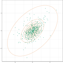
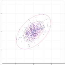
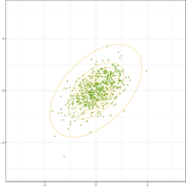
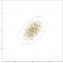
The $t_{p}(\mu,\Sigma;\nu)$ distribution has characteristic function as follows

Theorem 1

Let $X$ be a $p$-dimensional random vector having the multivariate $t$ distribution as per (1). Then the characteristic function of $X$ is given by

$$\phi_{X}(t)=\exp{(it^{\prime}\mu)}\frac{2}{\Gamma(\frac{\nu}{2})}\Big{(}\frac{i\nu t^{\prime}\Sigma t}{4}\Big{)}^{\frac{\nu}{4}}K_{\frac{\nu}{2}}(\sqrt{i\nu t^{\prime}\Sigma t}),$$ (2)

where $K_{\frac{\nu}{2}}(s)$ is the modified Bessel function of the second kind (Abramowitz & Stegun, 1964) of order $\nu/2$ and $\Gamma(z)=\int_{0}^{\infty}\exp{\{-x\}}x^{z-1}dx$ is the gamma function.

Proof

From definitions of the characteristic function of $X$ and the expectation of functions of $X$, we have $\phi_{X}(it)=E_{X}\{\exp{(it^{\prime}X)}\}=E_{Y,S}[\exp{\{it^{\prime}(\mu+Y\sqrt{\nu/S})\}}]=\exp{(it^{\prime}\mu)}E_{Y,S}\{\exp{(it^{\prime}Y\sqrt{\nu/S})}\}.$ But from the definition of joint expectations, $E_{Y,S}\{\exp{(it^{\prime}Y\sqrt{\nu/S})}\}=E_{S}\{E_{Y\mid S}[\exp{\{(it^{\prime}Y\sqrt{\nu/S})\}}]\}$. Also $Y$ is independent of $S$, so the inner conditional expectation is given by $E_{Y\mid S}[\exp{\{(it^{\prime}Y\sqrt{\nu/S})\}}]=\exp{\{{-i\nu t^{\prime}\Sigma t}/({2S})\}}$. We now use the result (see Bernardo & Smith, 1993, pages 119 and 431) that if $S\sim\chi^{2}_{\nu}$, then $W=1/S$ has the inverse-$\chi_{\nu}^{2}$ distribution with characteristic function given by

$$\phi_{W}(r)=\frac{2}{\Gamma(\frac{\nu}{2})}\Big{(}-\frac{ir}{2}\Big{)}^{\frac{\nu}{4}}K_{\frac{\nu}{2}}(\sqrt{-2ir}).$$ (3)

Then, $E_{S}[\exp{\{{-i\nu t^{\prime}\Sigma t}/({2S})\}}]$ is the same as evaluating $\phi_{W}(r)$ at $r=\nu t^{\prime}\Sigma t/2$. The theorem follows.

Corollary 1

Let $X$ be a $p$-dimensional random vector from the multivariate $t$-density $t_{p}(\mu,\Sigma;\nu)$. Let $X^{(q)}$ be the first $q(\leq p)$ coordinates in $X$. Then $X^{(q)}\sim t_{p}(\mu^{(q)},\Sigma^{(q\times q)};\nu)$, where $\mu^{(q)}$ is the vector with the first $q$ coordinates of $\mu$ and $\Sigma^{(q\times q)}$ is the $q\times q$ symmetric matrix containing the first $q$ rows and column entries of $\Sigma$.

Proof

Setting $t^{\prime}=(t_{1},t_{2},\ldots,t_{q},0,0,\ldots,0)$ in (2) yields the characteristic function that is uniquely that of the $t_{q}(\mu^{(q)},\Sigma^{(q\times q)},\nu)$ density and the result follows.

2.1.2 MBC with $t$-mixtures

MBC is an effective and principled method of obtaining groups of similar observations in a dataset. It scores over partitioning algorithms like $k$-means mainly in that it is not restricted by the inherent assumption of homogeneous spherically dispersed groups. Assuming spherically-dispersed groups when they are really non-spherical can lead to erroneous results (see Chattopadhyay & Maitra, 2017, for a comprehensive review on the pitfalls of using $k$-means when assumptions are not met.) In MBC (Melnykov & Maitra, 2010; McLachlan & Peel, 2000; Fraley & Raftery, 2002a) the observations $X_{1},X_{2},\ldots,X_{n}$ are assumed to be realizations from a K-component mixture model (McLachlan & Peel, 2000) with PDF

$$f(x;\theta)=\sum_{k=1}^{\textit{K}}\pi_{k}f_{k}(x;\eta_{k})$$ (4)

where $f_{k}(\cdot;\eta_{k})$ is the density of the $k$th group, $\eta_{k}$ the vector of unknown parameters and $\pi_{k}=Pr[x_{i}\in\mathit{G}_{k}]$ is the mixing proportion of the $k$th group, $k=1,2,\ldots,K$, and $\sum_{k=1}^{\textit{K}}\pi_{k}=1$. For convenience, we write $\theta$ as the set of of all the model parameters. The most popular mixture model is the Gaussian Mixture Model (GMM), where the component densities are assumed to be multivariate Gaussian $\phi(x;\mu_{k},\Sigma_{k})$ with mean $\mu_{k}$ and dispersion $\Sigma_{k}$. Imposing different constraints on the densities (mostly on the dispersion matrices) gives rise to a family of mixture models that are more parsimonious compared to the fully unconstrained model. The popular MCLUST GMM family of Fraley & Raftery (1998, 2002a) uses an eigen-decomposition of the component’s variance covariance matrices. Thus, they write $\Sigma_{k}=\lambda_{k}B_{k}\Lambda_{k}B_{k}^{T}$, where $\Lambda_{k}$ is a diagonal matrix with values proportional to the eigen values of $\Sigma_{k}$, $B_{k}$ denotes the matrix of eigen vectors of $\Sigma_{k}$ and $\lambda_{k}$ is the constant of proportionality. The MCLUST family  (Fraley & Raftery, 1998, 2002a) has 17 GMMs obtained by imposing certain constraints on $\lambda_{k}$, $B_{k}$ and $\Lambda_{k}$ and is implemented using the R (R Core Team, 2017) package MCLUST (Fraley & Raftery, 2002b; Fraley et al., 2012). Another useful class of mixture models is obtained when the component cluster densities are assumed to follow a multivariate t-distribution rather than a multivariate Gaussian distribution. Motivated by McLachlan & Peel (1998), these mixture models perform better than GMM when it is plausible for each group has some extreme observations. Andrews & McNicholas (2012) proposed a set of multivariate t mixture models(tMM) by imposing the same constraints as MCLUST plus additional constraints on $\nu$ to provide 24 multivariate tMMs. These models are implemented in the TEIGEN package (Andrews & McNicholas, 2015) in R (R Core Team, 2017).

The most common method of estimating the parameters of a mixture model is the Expectation Maximization (EM) Algorithm (Dempster et al., 1977; McLachlan & Krishnan, 2008), which is an iterative method for finding maximum likelihood estimates (MLEs) in incomplete data scenarios. Andrews & McNicholas (2012) used a variant of EM known as the Expectation Conditional Maximization (ECM) algorithm (Meng & Rubin, 1993) to estimate the parameters of the tMM. Faster modifications (Meng & Van Dyk, 1997; Chen & Maitra, 2011) exist but they have the same idea as ECM in that they replace the M-step of EM with a sequence of $D$ conditional maximization (CM) steps. Thus, the vector of parameters $\theta$ is partitioned into $D$ sub-vectors $\theta=(\theta_{1},\theta_{2},\ldots,\theta_{D})$ and the maximization done in $D$ steps, where the $d$th CM step maximizes the Q function (or the expected complete log likelihood function given the observations) over $\theta_{d}$ but while keeping the other sub-vectors fixed at some previous value. ECM is computationally more efficient than EM and also shares its desirable convergence properties (Meng & Rubin, 1993). We now outline ECM estimation in the context of $t$MMs.

Let $\zeta_{ik}$ be indicator variables that denote the cluster membership of the $i$th observation. Thus

$$\zeta_{ik}=\begin{cases}1,&\text{if the $i$th observation $x_{i}$ belongs to the $k$th group}\\ 0,&\text{otherwise}.\end{cases}$$ (5)

Note that $\zeta_{ik}$s are unobserved and estimating them is the major objective of MBC. In the context of the $t$MM, there is an additional set of missing values $v_{ik},i=1,2,\ldots,n;k=1,2,\ldots,K$ that are realizations from the Gamma density with PDF

$$\gamma(v_{ik};\nu_{k}/2,\nu_{k}/2)=\frac{\nu_{k}^{\frac{\nu_{k}}{2}}{v_{ik}}^{\frac{\nu_{k}}{2}-1}\exp{({-\frac{\nu_{k}v_{ik}}{2}})}}{2^{\frac{\nu_{k}}{2}}\Gamma(\frac{\nu_{k}}{2})}.$$ (6)

Then for the $t$MM the complete data loglikelihood function can be written as

$$\begin{split}\ell(&\pi,\mu,\Sigma,\zeta)\\ &=\sum_{k=1}^{K}\sum_{i=1}^{n}\zeta_{ik}\log\{\pi_{k}\phi(x_{i};\mu_{k},\Sigma_{k}/v_{ik})\gamma(v_{ik};\nu_{k}/2,\nu_{k}/2)\}\\ \end{split}$$ (7)

where $\nu_{k}$ denotes the degrees of freedom of the $t$-density for the $k$th group, $\phi$ denotes Gaussian density with mean $\mu_{k}$ and variance $\Sigma_{k}/v_{ik}$. The $t$MM likelihood is maximized through the following steps:

1. Initialization. Let $\{(\pi_{k}^{\circ},\mu_{k}^{\circ},\Sigma_{k}^{\circ},\nu_{k}^{\circ});k=1,2,\ldots,K\}$ be the initializing parameters.

2. E-step updates. The component weights $v_{ik}$ and the group indicator variables $\zeta_{ik}$ are updated as

   $$\hat{v}_{ik} = \frac{\nu_{k}^{\circ}+p}{\nu_{k}^{\circ}+(x_{i}-\mu_{k}^{\circ})^{T}\Sigma_{k}^{\circ-1}(x_{i}-\mu_{k}^{\circ})}$$

   $$\hat{\zeta}_{ik} = \frac{\pi_{k}^{\circ}f_{t}(x_{i};\mu_{k}^{\circ},\Sigma_{k}^{\circ},\nu_{k}^{\circ})}{\sum_{k=1}^{K}\pi_{k}^{\circ}f_{t}(x_{i};\mu_{k}^{\circ},\Sigma_{k}^{\circ},\nu_{k}^{\circ})}$$

   where $f_{t}(x_{i};\mu_{k}^{\circ},\Sigma_{k}^{\circ},\nu_{k}^{\circ})$ denotes a multivariate t-density with mean $\mu_{k}$, dispersion matrix $\Sigma_{k}$ and degrees of freedom $\nu_{k}$.

3. CM-step 1. The first CM step updates the component means $\mu_{k}$s and the prior probabilities $\pi_{k}$s:

   $$\hat{\pi}_{k} = \frac{\hat{n}_{k}}{n}$$

   $$\hat{\mu}_{k} = \frac{\sum_{i=1}^{n}\hat{\zeta}_{ik}\hat{v}_{ik}x_{i}}{\sum_{i=1}^{n}\hat{\zeta}_{ik}\hat{v}_{ik}}$$

   where $\hat{n}_{k}=\sum_{i=1}^{n}\hat{\zeta}_{ik}$. Additionally, if the constraint $\nu_{k}\equiv\nu$ is imposed upon the degrees of freedom of each group, then $\hat{\nu}$ is updated here by solving the equation

   $$\begin{split}1-\psi\Big{(}\frac{\hat{\nu}}{2}\Big{)}+\frac{1}{n}&\sum_{k=1}^{K}\sum_{i=1}^{n}\hat{\zeta}_{ik}(\log\hat{v}_{ik}-\hat{v}_{ik})+\log\Big{(}\frac{\nu}{2}\Big{)}\\ &+\psi\Big{(}\frac{\nu^{\circ}+p}{2}\Big{)}-\log\Big{(}\frac{\nu^{\circ}+p}{2}\Big{)}=0.\end{split}$$ (8)

   where $\hat{\nu}$ denotes the updated degrees of freedom and $\nu^{\circ}$ denotes the current estimate.

4. CM-step 2. This step updates the $\Sigma_{k}$s and varies accordingly as per constraints imposed in the modeling. For example, setting $\Lambda_{k}=\Lambda$ and $B_{k}=B$ yields the updates

   $$\hat{\lambda}_{k}=\frac{1}{p\hat{n}_{k}}trace\Big{(}S_{k}H^{-1}\Big{)}$$ (9)

   where $S_{k}=\frac{1}{\hat{n}_{k}}\sum_{i=1}^{n}\hat{\zeta}_{ik}\hat{v}_{ik}{||x_{i}-\hat{\mu}_{k}||}^{2}$ and $H=B\Lambda B^{T}$. In order to update $B$ and $\Lambda$, $H$ is first updated using using

   $$H=\frac{\frac{1}{\lambda_{k}}\sum_{k=1}^{K}S_{k}}{{|\frac{1}{\lambda_{k}}\sum_{k=1}^{K}S_{k}|}^{\frac{1}{p}}}$$ (10)

   Now the updated $B$ and $\Lambda$ are obtained from (10).

5. Alternate between the E- and CM-steps till convergence.

After obtaining the final estimates of the parameters, the $i$th data point $X_{i}$ is assigned to the class for which the converged E-step posterior probability is the highest, that is $X_{i}$ is assigned to class $k$ where $k=\operatorname*{arg\,max}_{l}\hat{\zeta}_{il}$.

Our $t$-mixtures MBC ($t$MMBC) formulation above assumes a known number of components $K$. With unknown $K$, a popular approach of finding it is the Bayesian Information Criterion (BIC) (Schwarz, 1978) that subtracts $(m\log n)/2$ from the maximized log-likelihood (obtained from the converged ECM), with $m$ the number of unconstrained parameters in the fitted $K$-component $t$MM.  (See Chattopadhyay & Maitra, 2017, for a detailed review of BIC.)

2.1.3 Illustration

The purpose of this section is to demonstrate using a simulated dataset, potential pitfalls in fitting a GMM on data that are plausibly realizations from a multivariate tMM. For this purpose, we simulated three 4-component multivariate tMMs having an approximate generalized overlap (Maitra, 2010; Melnykov & Maitra, 2011) of $\ddot{\omega}=0.01$ and $\nu=5,15,25$ degrees of freedom. The generalized overlap measure is an effective way of summarizing the overlap matrix $\Omega$ of Maitra & Melnykov (2010) which is a $K\times K$ matrix whose $(i,j)th$ element contains the sum of misclassification probabilities between $i$th and $j$th clusters. The generalized overlap summarizes this matrix and is defined as $\ddot{\omega}=(\lambda_{(1)}-1)/(K-1)$ where $\lambda_{(1)}$ is the largest eigen value of $\Omega$. Small values of $\ddot{\omega}$ are likely to indicate more distinct groupings. (See also Chattopadhyay & Maitra, 2017, for further details.). The MixGOM() function in the R package MixSim (Melnykov et al., 2012) can be adapted in the same manner as Melnykov & Maitra (2011) to obtain realizations from a multivariate $t$MM with a specified $\ddot{\omega}$.

We fitted both GMM and tMM to the datasets, with optimal number of groups determined using BIC, and results displayed in Fig. 2. For $\nu=5$ and $\nu=10$ fitting a GMM gives the optimal number of clusters to be five and four respectively but for tMM the optimum number of clusters were correctly chosen as three in both cases. For $\nu=25$, BIC identified the number of clusters as three for both class of models.

Figure 2: Simulated datasets from a bivariate tMM with $\nu=5,10,25$ in the top, middle and bottom panels, and clustering obtained using GMM (left-hand panel) and $t$MM (right-hand panel). In all figures, plotting character indicates true classification while color indicates estimated grouping.

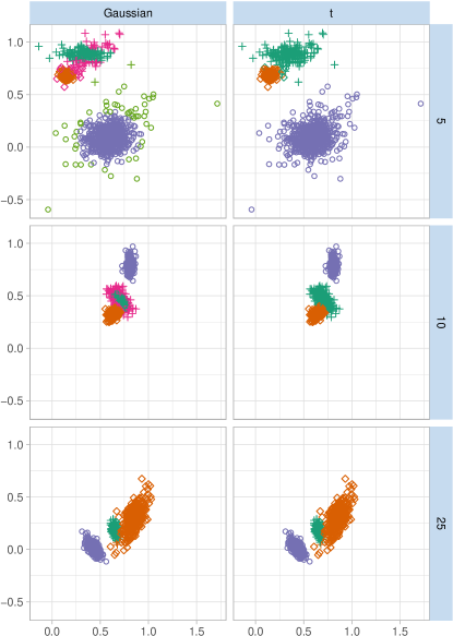
For numerical assessment of clustering performance,we computed the Adjusted Rand index ($\mathcal{R}$) after fitting each of the two models to the data. As also explained by Maitra (2001), the Rand index (Rand, 1971) is a measure of similarity between two different clusterings and is calculated as follows. Suppose that for a given data set $\mathcal{D}$ having $n$ elements there exists two different partitions $P_{1}$ and $P_{2}$ by two different algorithms. Let $a_{1}$ denote the number of pairs of object in $\mathcal{D}$ that are in the same group in both partitions $P_{1}$ and $P_{2}$, and $a_{2}$ the number of pairs of objects in $\mathcal{D}$ that are in different groups. Then the Rand index is defined as $(a_{1}+a_{2})/\binom{n}{2}$. The Rand Index takes values between 0 and 1. The Adjusted Rand Index (Hubert & Arabie, 1985) is obtained by correcting Rand Index for chance grouping of elements and can take values between $-\infty$ and $1$. We analyzed the quality of clustering for both GMM and $t$MM by comparing the clustering results with the true class indicators through $\mathcal{R}$ in order to demonstrate issues of using a GMM model for clustering a data supposedly originating from a tMM, that is from a mixture model with potentially heavier tails. The results are presented in Table 1.

Table 1: Adjusted Rand Indices obtained by clustering three datasets simulated from a 3-component tMM with $\nu$ equal to 5, 10 and 25 using a Gaussian mixture model and a $t$ mixture model.

$\nu$	Gaussian	$t$
5	0.84	0.99
10	0.79	0.99
25	0.99	0.99

Both Fig. 2 and Table 1 clearly indicate that a tMM gives a better fit that a GMM, for smaller $\nu$. For $\nu=25$, the difference is negligible but enough to prove that tMM wins over GMM. Our examples here illustrate the value of considering a tMM when the underlying groups are potentially thicker-tailed.

2.2 Variable Selection in Clustering

(a) Pairwise scatterplots, estimated marginal densities and pairwise correlations of simulated datasset.

(b) $\hat{K}=2$, $\mathcal{R}=0.37$

(c) $\hat{K}=2$, $\mathcal{R}=0.37$

(d) $\hat{K}=4$, $\mathcal{R}=0.82$

(e) Two views of clustering using all three dimensions: $\hat{K}=5$, $\mathcal{R}=1.0$

Figure 3: Result of clustering (a) data simulated from a three-dimensional 5-component GMM using (b, c, d) two and (e) all three variables.

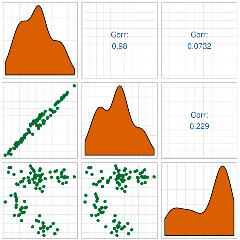
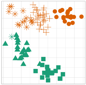
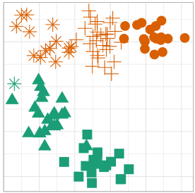
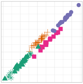
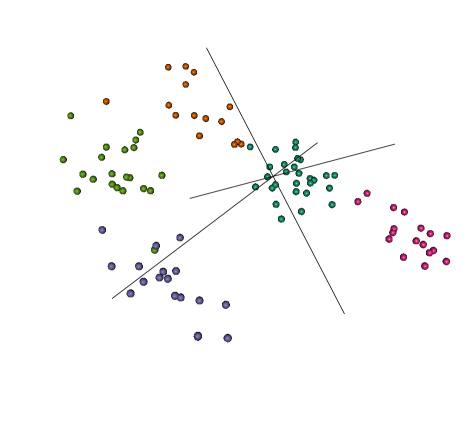
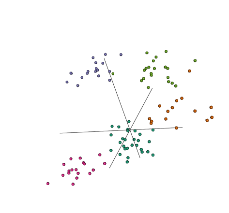
Selection of relevant variables is a very important issue in clustering. Incorporating redundant information can degrade overall clustering performance producing less distinct groups (Chattopadhyay & Maitra, 2017). In the same way, exclusion of variables having relevant information also degrades the overall quality of clustering. We illustrate this problem (Fig. 3) by means of a simulated three-dimensional dataset drawn from a GMM with $K=5$ true and very well separated components ($\ddot{\omega}=10^{-5}$) and with marginal distributions and pairwise scatterplots as shown in the diagonal and lower triangle of the matrix of plots in Fig. 3a. The upper triangle of these matrix displays the correlation between each pairs of variables. Thus the first two of the three variables have a very high (almost linear) pairwise correlation of 0.98, while the other two pairs have little to modest correlations between them. It is tempting to surmise that one of the first two dimensions are nearly redundant and dropping one of them would not have much of an effect on the quality of clustering. We test this assertion by performing GMMBC (with BIC used to determine the optimal number of groups) on the dataset using each of the three distinct pairs of variables. Figs 3b-3d display the results of clustering each pair of coordinates, with colors representing the obtained clustering and character the true grouping. Including either one of the two seemingly redundant variables with the third variable identifies only two groups and a partitioning (Figs 3b and 3c) that hardly matches the true with an adjusted Rand index ($\mathcal{R}$) of 0.37. Interestingly, clustering the two seemingly redundant variables (and ignoring the third) does better, identifying four groups and with $\mathcal{R}=0.82$. However, this is still a far cry from the perfect partitioning that is obtained when all three coordinates are used in GMMBC with BIC to determine the optimal number of groups. Therefore, it is important to consider the relevant variables in clustering. This fact becomes more important in the light of attempts by many researchers to cluster GRBs using, for instance, only the duration variables. This example also demonstrates that two variables having correlations even as high as 0.98 are not necessarily redundant and should be carefully analyzed before arriving at decisions on their inclusion or exclusion in analysis. Raftery & Dean (2006) proposed a method for selecting variables containing the most relevant clustering information by recasting the variable selection problem in terms of model selection, where comparison of the models is done via BIC. (refer to Chattopadhyay & Maitra, 2017, for a thorough review on variable selection.)

2.3 Measuring Distinctiveness of Partitioning Through the Overlap

Chattopadhyay & Maitra (2017) explain that an overlap measure can be used to indicate the extent to which clusters obtained through a method are distinct from one another. We refer to that paper for further details, but note that they adopt Maitra & Melnykov (2010)’s definition of the pairwise overlap between two groups as the sum of their misclassification probabilities. To provide a sense of these pairwise overlap measures, we illustrate three two-dimensional examples in Fig. 4. (For ease of display and understanding, we use two dimensions here, but the general idea is the same for all dimensions.) In each case, we used the MixSim package to sample 1000 observations from two-component GMMs but with pairwise overlaps of $\omega=10^{-3}$, 0.05 and 0.1, respectively.

(a) $\omega=10^{-3}$

(b) $\omega=0.05$

(c) $\omega=0.1$

Figure 4: Sample realizations, along with estimated contour densities, from two-component $t$MMs with three different overlap values.

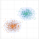
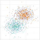
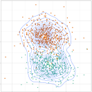
In each figure, we display the observations from each group by means of color and character and also provide an estimated bivariate density through a contour plot. The contours are totally separated for the data with negligible pairwise overlap (Fig. 4a). This separation decreases with increasing overlap (Figs 4b and 4c) and the groups become less distinct.

2.4 Classification

The objective of classification is to classify a new observation to one of $K$ well-defined groups. Classification is a supervised learning method that uses training data to determine a rule that classifies a new observation to one of $K$ groups. Bayes’ rule is often used to obtain classification rules in the model-based context. Here an observation $x$ is assigned to the $l$th group if the posterior probability of $x$ belonging to the $i$th group is the highest amongst all groups under considerations. Thus, the decision rule is to classify $x$ to group $i$ if $\pi_{i}f_{i}(x)>\pi_{k}f_{k}(x)$ for all $k\neq i$, where $\pi_{j}$ is the prior probability that an observation belongs to the $j$th group and $f_{j}(x)$ denotes the PDF of the $j$th group at $x$ (see Johnson & Wichern, 1988, for more details.). In case of tMM $f_{i}(x)$ denotes a multivariate-$t$ PDF. Our proposal is to cluster the observations for which all parameters are observed and to use the estimated parameters to classify the GRBs for which not all parameters are observed. We will use the above methods for developing our classification rule for observations with missing records.

3 Cluster Analysis of GRBs

The BATSE catalogue is widely used for analysis of GRBs and has temporal and spectral information of GRBs from 1991 to 2000. A few of the parameters have been of interest to researchers for grouping GRBs. These are:

$T_{50}$:

the time by which 50% of the flux arrive.

$T_{90}$:

the time by which 90% of the flux arrive.

$P_{64}$, $P_{256}$, $P_{1024}$:

the peak fluxes measured in bins of 64, 256 and 1024 ms, respectively.

$F_{1}$, $F_{2}$, $F_{3}$, $F_{4}$:

the four time-integrated fluences in the 20-50, 50-100, 100-300, and $>$ 300 keV spectral channels, respectively.

Apart from these nine parameters three more composite parameters are of interest to researchers (Mukherjee et al., 1998). These are:

$F_{t}$=$F_{1}+F_{2}+F_{3}+F_{4}$:

the total fluence of a GRB.

$H_{32}=F_{3}/F_{2}$:

measure of spectral hardness using the ratio of $F_{2}$ and $F_{3}$.

$H_{321}=F_{3}/(F_{1}+F_{2})$:

measure of spectral hardness based on the ratio of channel fluences $F_{1},F_{2},F_{3}$.

The current (BATSE 4Br) catalogue contains revised locations of 208 bursts from the BATSE 4B Catalog along with 515 bursts observed between September 20 1994 and August 29 1996 apart from the bursts present in the BATSE 3B Catalog. Many parameters, largely in the four time-integrated fluences $F_{1}$, $F_{2}$, $F_{3}$ and especially $F_{4}$, have zeroes recorded that can be regarded as missing (Chattopadhyay & Maitra, 2017). Consequently, the derived variables are also missing for these GRBs. So the BATSE 4Br catalog has 1599 GRBs (among 1973 GRBs) containing complete information on all the nine original (plus three derived) variables. Most authors have used a very subset of these 12 variables for their analysis. This led us to wonder whether the nine original variables contains relevant information that might improve the quality of the clustering to give more coherent groups. We thus analyzed 1599 GRBs from the BATSE 4Br catalogue having complete information on the nine original variables with MBC using mixtures of t-densities. Further, we wondered if the five groups identified by Chattopadhyay & Maitra (2017) were only because the groups identified were constrained to be Gaussian and so had thinner tails, while there really were fewer groups with thicker tails, that is a scenario reminiscent of the situation in  2. Therefore, we reanalyzed the BATSE data using all nine parameters and $t$MMBC.

We first briefly discuss the univariate and bivariate relationships between the nine original parameters in the BATSE 4Br catalogue.

Figure 5: A matrix of scatterplots (the lower triangle), density plots ( the diagonal) and correlation coefficients(the upper triangle) of the nine parameters $T_{50}$, $T_{90}$, $P_{64}$ $P_{256}$, $P_{1024}$, $F_{1}$, $F_{2}$, $F_{3}$ and $F_{4}$ using 1599 GRBs of the BATSE 4Br catalogue. All displays are in the logarithmic scale.

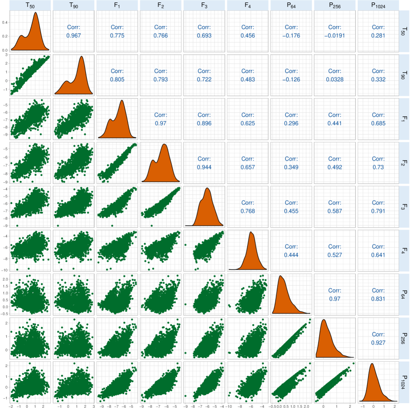
Fig. 5 displays the bivariate relationships between the nine original variables of the BATSE 4Br catalogue along with the univariate density plots of the nine parameters. The two duration variables $\log_{10}T_{50}$ and $\log_{10}T_{90}$ exhibit a very high positive association amongst themselves. Similar behavior is exhibited by the three peak fluxes $\log_{10}P_{64}$, $\log_{10}P_{256}$ and $\log_{10}P_{1024}$. Fluence $\log_{10}F_{1}$ shows a very high positive association with fluences $\log_{10}F_{2}$ and $\log_{10}F_{3}$ and a high positive association with $\log_{10}F_{4}$. Fluence $\log_{10}F_{2}$ exhibits a very high positive association with $\log_{10}F_{3}$ and a high positive association with $\log_{10}F_{4}$ that also has a high positive association with $\log_{10}F_{3}$. Duration $\log_{10}T_{50}$ exhibits a high positive association with fluences $\log_{10}F_{1}$, $\log_{10}F_{2}$ and $\log_{10}F_{3}$ and a moderate positive association with $\log_{10}F_{4}$. $\log_{10}T_{90}$ behaves similar to $\log_{10}T_{50}$ except that it shows a very high positive association with $\log_{10}F_{1}$. Fig. 3 has also pointed out through the scatterplots the limitations that are posed on grouping using only one or two variables, thus pointing out the importance of using more than two variables for clustering. We now perform cluster analysis on the $1599$ GRBs using the nine original parameters (in logarithmic scale), that is $\log_{10}T_{50}$, $\log_{10}T_{90}$, $\log_{10}F_{1}$, $\log_{10}F_{2}$, $\log_{10}F_{3}$, $\log_{10}F_{4}$, $\log_{10}P_{64}$, $\log_{10}P_{256}$ and $\log_{10}P_{1024}$.

3.1 Clustering GRBs Using All Observed Parameters

We first perform $t$MMBC using 1599 GRBs from the BATSE 4Br catalogue and then classify the GRBs with incomplete information to the groups obtained using the $t$MMBC.

3.1.1 $t$MMBC with all nine parameters

We check for redundancy among the nine parameters $\log_{10}T_{50}$, $\log_{10}T_{90}$, $\log_{10}P_{64}$, $\log_{10}P_{256}$, $\log_{10}P_{1024}$, $\log_{10}F_{1}$, $\log_{10}F_{2}$, $\log_{10}F_{3}$, $\log_{10}F_{4}$ using model-based variable selection. The results obtained (Table 2) do not show redundancy among these nine parameters. However, there is redundancy beyond these nine variables, because the derived variables are linearly related to the nine parameters. We thus performed $t$MMBC on the nine original variables using the TEIGEN package in R and determined $K$ from amongst $\{1,2,\ldots,9\}$ using BIC – indeed,

Table 2: Results of forward and backward-variable selection for determining redundancy among $\log_{10}T_{90}$, $\log_{10}T_{50}$, $\log_{10}P_{64}$, $\log_{10}P_{1024}$, $\log_{10}P_{256}$, $\log_{10}F_{3}$, $\log_{10}F_{2}$, $\log_{10}F_{1}$, $\log_{10}F_{4}$ for MBC.

Step	Variable	Step Type	BIC Difference	Decision
1	$\log_{10}T_{90}$	Add	452.95	Accepted
2	$\log_{10}T_{50}$	Add	395.74	Accepted
3	$\log_{10}P_{64}$	Add	181.35	Accepted
4	$\log_{10}P_{64}$	Remove	181.73	Rejected
5	$\log_{10}P_{1024}$	Add	1636.98	Accepted
6	$\log_{10}T_{90}$	Remove	391.06	Rejected
7	$\log_{10}P_{256}$	Add	1266.77	Accepted
8	$\log_{10}T_{90}$	Remove	235.84	Rejected
9	$\log_{10}F_{3}$	Add	540.03	Accepted
10	$\log_{10}T_{90}$	Remove	243.47	Rejected
11	$\log_{10}F_{2}$	Add	509.78	Accepted
12	$\log_{10}T_{90}$	Remove	95.59	Rejected
13	$\log_{10}F_{1}$	Add	312.38	Accepted
14	$\log_{10}T_{90}$	Remove	45.00	Rejected
15	$\log_{10}F_{4}$	Add	113.55	Accepted
16	$\log_{10}F_{4}$	Remove	16.09	Rejected

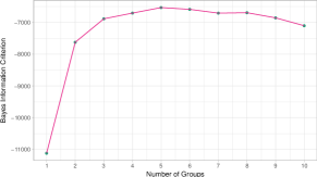
Fig. 6 indicates overwhelming evidence in favor of a five-component $t$MM, with a difference of greater than 10 than for other $K$, which as per  Kass & Raftery (1995), constitutes very strong evidence. The results obtained mirror those of Chattopadhyay & Maitra (2017) which also found five groups upon using GMMBC and six parameters.

$K$	BIC
1	-11120.1
2	-7625.3
3	-6885.8
4	-6705.8
5	-6532.6
6	-6588.5
7	-6707.0
8	-6693.9
9	-6856.2

(a)

(b)

Figure 6: BIC for each $K$ upon performing $t$MMBC of the 1599 GRBs in the BATSE 4Br catalogue.

A reviewer asked why we did not simply eliminate variables that did not have much apparent additional information because they were highly correlated with other variables. We refer back to the example of Fig. 3 in Section 3 and note that there also we had very high correlations (0.98) between two variables, but both were needed to be included with the third variable for good clustering performance. The fact that the correlation between any pair is high does not necessarily mean that one of the variables in the pair is redundant for clustering and can simply be dropped. Indeed, it is possible that there is more redundancy of the variables with regard to defining some group and not in the case of others. We return to this point again in Section 3.1.1, but note our preference for using the data to systematically inform us of relevant and irrelevant variables for clustering. Our formal variable selection algorithm establishes the relevance of all nine parameters. Also as mentioned in Section 2.1.2, the TEIGEN (and MCLUST) family allows for restricted dispersion matrices with the choice governed by BIC that penalizes more complicated (i.e. less restricted) models.

Validity of obtained groupings

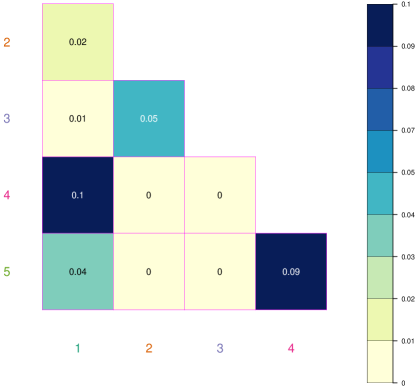
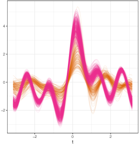
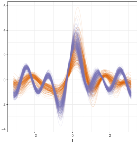
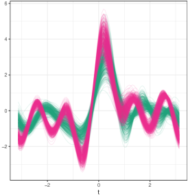
We calculate the empirical pairwise overlap by fitting a GMM as described in the the MixSim package (Melnykov et al., 2012). The overlap map of Fig. 7 shows the distinctness of the five groups obtained using $t$MMBC. It is evident that the Group 4 have very small overlap with both Groups 2 and 3. On the other hand, Groups 1 and 4 have the highest overlap, while the pairwise overlap measures between Groups 1, 2 and 3 are moderate. The overlap map indicates that the clusters obtained are quite well-separated and so our results find five GRB sub-populations that are more distinct than Chattopadhyay & Maitra (2017). In order to provide a clearer understanding of the figures in the overlap map we provide a visual representation of the three pairs of groups having approximate overlaps of 0, 0.1 and 0.05, using an Andrews plot (Andrews, 1972) in Fig. 8 that provides an

Figure 7: Pairwise overlap measures between the $k$th and the $l$th groups obtained by our five-component $t$MMBC solutions.

effective way to visualize multivariate data. In Andrews plot, a realization $x=(x_{1},x_{2},\ldots,x_{p})^{T}$ is represented by a curve $f_{x}(t)$ in argument $t$ $(-\pi\leq t\leq\pi)$ where $f_{x}(t)$ defines a finite Fourier series

$$f_{x}(t)=\frac{x_{1}}{\sqrt{2}}+x_{2}\sin t+x_{3}\cos t+x_{4}\sin 2t+x_{5}\cos 2t+\ldots$$ (11)

Thus each observation is represented as a curve in $(-\pi,\pi)$. (For a detailed review of Andrews curves, see Khattree & Naik, 2002). In Fig. 8a the two groups represented by the curves of different colours are much more distinct than those in figures 8b and 8c. Indeed, in none of the cases do the curves of different colours track together: there is separation at some point or the other on every curve. Similar comparison curves obtained from the other pairs of groups show that our five groups are well-separated compared to the groups obtained by Chattopadhyay & Maitra (2017).

(a) Groups 2 and 4 GRBs

(b) Groups 2 and 3 GRBs

(c) Groups 1 and 4 GRBs

Figure 8: Andrews plot of observations in (a) Groups 2 and 4 having negligible pairwise overlap, (b) Groups 2 and 3 having overlap of 0.05 and (c) Groups 1 and 4 having overlap of 0.1

Also, the generalized overlap (see Chattopadhyay & Maitra (2017)) for the five component solutions is 0.05 which is much less than the 0.10 obtained for five-component GMMBC solution in Chattopadhyay & Maitra (2017) that adds support to the fact the groups obtained here are more distinct than than those obtained by Chattopadhyay & Maitra (2017).

A reviewer wondered whether our five-cluster results were by chance and whether accounting for variability in the estimated groupings and parameters would yield different, perhaps more conservative, results. We note that BIC chose five clusters and did so, as per Kass & Raftery (1995) decisively, with a difference of over 10 than all other models and components under consideration. To further investigate the strength of this result, we also used a nonparametric bootstrap technique to estimate the distribution of the number of kinds of GRBs in the BATSE catalog. Specifically, we used 1000 bootstrap replicates of the dataset, with each replicate obtained by sampling with replacement 1599 records from the complete dataset. For each replicate, we fit $t$MMs in the same manner as in Section 3.1 and used BIC to select the order of the model from among $K=2,3,4,5$. All 1000 bootstrap replicates chose the five-component cluster model, providing confidence in our findings that there are five ellipsoidal sub-populations of GRBs in the BATSE 4Br catalogue.

A second reviewer asked us to clarify that our nonparametric bootstrap procedure as implemented above only provides an estimate of the number of clusters that is selected using BIC. It, of course, does not provide a $p$-value of the hypothesis that $K=5$ is the smallest number of clusters compatible with the data. To address this latter question, we could implement a parametric bootstrap procedure whereby the bootstrap samples are drawn from the $K_{*}$-component $t$-mixture distribution fitted to the original data. The $p$-value of the test of $H_{0}:K=K_{*}$ versus the alternative hypothesis $H_{a}:K=K^{*}$ could be approximated calculated on the basis of the bootstrap replications of the likelihood ratio test statistic formed for each bootstrap sample after the fitting of $K_{*}$ and $K^{*}$ $t$-component mixture densities densities to it. (For testing the competing hypothesis of two against five groups, for instance, we would have $K_{*}=2$ and $K^{*}=5$ in the above specification. For testing that $K=5$ is the smallest number of groups compatible with the data, we would set $K_{*}=5$ and $K^{*}=K_{1}>5$.) Indeed, this is a very computationally intensive procedure requiring multiple initializations and fittings for each of the pairs of models posited in the two competing hyptheses.

Analysis of Results

Figure 9: Parallel coordinate plot of the 1599 BATSE 4Br GRBs colored as per their group indicators. The solid lines represent the group medians for each of the nine variables displayed. Variables are in the logarithmic scale.

Table 3: Number of GRBs in each of the five groups obtained using $t$MMBC.

Group	1	2	3	4	5
Number of observations	360	160	237	479	363

Table 4: Mean (top row) and median (bottom row) parameter values for each of the five $t$MMBC groups. The figures in parenthesis are (top row) the standard error of the mean and (bottom row) the group inter-quartile range of the observations in that parameter.

$k$	$\log T_{50}$	$\log T_{90}$	$\log F_{1}$	$\log F_{2}$	$\log F_{3}$	$\log F_{4}$	$\log P_{64}$	$\log P_{256}$	$\log P_{1024}$
1	0.72(0.03)	1.10(0.03)	-6.87(0.03)	-6.76(0.03)	-6.30(0.03)	-5.97(0.04)	0.11(0.02)	0.00(0.02)	-0.16(0.02)
	0.76(0.92)	1.15(0.95)	-6.85(0.82)	-6.76(0.63)	-6.29(0.67)	-5.94(0.87)	0.04(0.44)	-0.07(0.46)	-0.20(0.46)
2	-0.62(0.07)	-0.07(0.07)	-7.98(0.05)	-7.77(0.04)	-7.05(0.04)	-6.42(0.05)	0.43(0.03)	0.13(0.03)	-0.36(0.04)
	-0.86(1.06)	-0.09(1.25)	-8.00(0.75)	-7.82(0.62)	-7.15(0.68)	-6.49(0.93)	0.36(0.36)	0.02(0.46)	-0.44(0.60)
3	-0.74(0.02)	-0.37(0.02)	-7.90(0.03)	-7.61(0.02)	-6.82(0.02)	-6.49(0.05)	0.50(0.03)	0.32(0.02)	-0.13(0.02)
	-0.72(0.41)	-0.35(0.48)	-7.90(0.49)	-7.64(0.46)	-6.86(0.44)	-6.39(0.83)	0.43(0.51)	0.26(0.44)	-0.18(0.44)
4	1.24(0.02)	1.67(0.02)	-6.27(0.02)	-6.18(0.02)	-5.78(0.02)	-5.86(0.03)	0.13(0.01)	0.07(0.01)	0.01(0.01)
	1.20(0.62)	1.66(0.51)	-6.25(0.60)	-6.17(0.58)	-5.80(0.56)	-5.80(0.81)	0.12(0.31)	0.06(0.34)	0(0.35)
5	0.88(0.03)	1.43(0.03)	-5.91(0.03)	-5.76(0.03)	-5.27(0.03)	-5.17(0.04)	0.82(0.02)	0.78(0.02)	0.69(0.02)
	0.92(0.68)	1.46(0.66)	-5.90(0.71)	-5.77(0.69)	-5.26(0.81)	-5.14(1.14)	0.75(0.57)	0.72(0.57)	0.63(0.56)

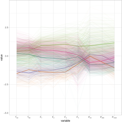
Table 3 provides the number of observations in each group, with the color for the group indicators matching the color of the groups in all figures to provide for easy cross-referencing. We see that Groups 1 and 4 contain the highest number of GRBs while Group 2 contains the lowest number of GRBs. Table 4 also lists the estimated means of the five groups. The standard errors of the estimated means for the five groups are also provided in the parenthesis corresponding to each estimate. A more detailed visual representation is provided by Fig. 9 which displays the five groups via a parallel coordinate plot(Inselberg, 1985; Wegman, 1990; Chattopadhyay & Maitra, 2017).

Most authors have used the duration variable $T_{90}$ to describe the group properties of GRBs while some have used fluences $F_{1}-F_{4}$ along with duration. Mukherjee et al. (1998) used total fluence $F_{t}=F_{1}+F_{2}+F_{3}+F_{4}$ and hardness ratio $H_{321}=F_{3}/F_{1}+F_{2}$ along with $T_{90}$ to describe the properties of their groups, a scheme that was also adopted by Chattopadhyay & Maitra (2017). We follow this scheme to describe our groups using the three properties duration-total Fluence-Spectrum. Using this rule the five groups of Chattopadhyay & Maitra (2017) were intermediate-faint-intermediate, long-intermediate-soft, intermediate-intermediate-intermediate, short-faint-hard and long-bright-intermediate. This same paradigm classifies our five $t$MMBC-obtained groups as long-intermediate-intermediate, short-faint-intermediate, short-faint-soft, long-bright-hard and long-intermediate-hard.

For a further study of the five groups, we take a closer look at the duration variable $\log_{10}T_{90}$. This variable also facilitates comparison of our results to those obtained in Chattopadhyay & Maitra (2017) and other authors such as Mukherjee et al. (1998) who have used $\log_{10}T_{90}$ along with other derived variables such as $\log_{10}F_{t}$. Our fourth and fifth group contains the bursts of highest duration (around $47s$ and $27s$ respectively). Typically the bursts from these two groups and the first group are designated as long-duration bursts ($T_{90}>2s$) following the popular classification scheme of classifying bursts with duration less than $2s$ as short duration bursts and bursts greater than $2s$ as long duration bursts (Chattopadhyay et al., 2007). The second and third groups consist of bursts of shortest duration (around $0.4s$ and $0.7s$ respectively) and will be classified as short duration bursts ($T_{90}<2s$). The standard errors of the estimated means are not large and show that the estimated means of the groups are distinct.

We also compared our $t$MMBC grouping with the GMMBC grouping of Chattopadhyay & Maitra (2017) by means of a cross classification table (Table 5).

Table 5: Number of 1599 GRBs assigned to each of the groupings by $t$MMBC using the nine original variables (Grouping I) and GMMBC of Chattopadhyay & Maitra (2017) using three original variables ($\log_{10}T_{50}$, $\log_{10}T_{90}$, $\log_{10}P_{256}$) and three derived variables $\log_{10}F_{t}$, $\log_{10}H_{32}$, $\log_{10}H_{321}$.

		Grouping I (New groupings)
		1	2	3	4	5	Total
Grouping II	1	86	50	14	24	0	174
	2	5	57	25	2	60	149
	3	45	48	198	0	1	292
	4	186	5	0	319	41	551
	5	38	0	0	134	261	433
	Total	360	160	237	479	363

The high values in the diagonal (with the exception for Group 2) indicates that the grouping structure in both the cases agrees well for both the analyses with the highest agreement being noted in the Group 4.

(a) Group 1

(b) Group 2

(c) Group 3

(d) Group 4

(e) Group 5

Figure 10: Variances and displays of the estimated correlations for each of the five groups obtained from the five-component MBC solution using t mixtures for the 1599 GRBs. For each group, the off-diagonal elements display correlation between the variables while the diagonals display the variances. Both correlations and variances are calculated for the variables in the base-10 logarithmic scale.

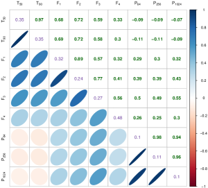
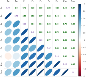
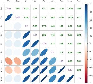
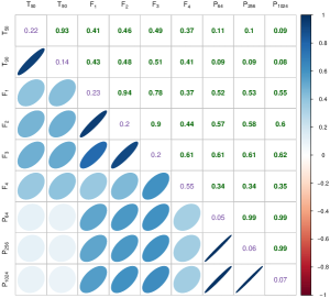
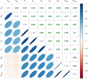
In order to facilitate further study of the group structures we calculated the correlations between the nine classes for each of the five groups (Fig. 10). The diagonals of each correlation plot display the estimated variance of the five groups obtained by $t$MMBC. The upper triangular portion of each correlation plot displays the correlation between the variables, while the lower triangular part provides a diagrammatic representation of the correlations in the upper triangular part [e.g. the (2,1)th cell displays the correlation between $\log_{10}T_{50}$ and $\log_{10}T_{90}$ diagrammatically, while the (1,2)th cell displays the numerical value]. The duration variables $\log_{10}T_{50}$ and $\log_{10}T_{90}$ display very high positive association in all five groups. Duration $\log_{10}T_{50}$ and fluence $\log_{10}F_{1}$ have a high positive association in Group 1 and moderate positive association in Groups 2, 4 and 5. In Group 3, they have very low positive association. The other fluences $\log_{10}F_{2}$, $\log_{10}F_{3}$ and $\log_{10}F_{4}$ also exhibit similar linear relationships with $\log_{10}T_{50}$ for the five groups except that $\log_{10}F_{4}$ shows a moderate positive association in Group 1. Duration $\log_{10}T_{90}$ has a high positive association with $\log_{10}F_{1}$ in Group 1. In Groups 2, 4 and 5 they display a moderate positive association and a weak positive association in Group 3 . Also, $\log_{10}T_{90}$ displays a moderately positive association with fluence $\log_{10}F_{2}$ in Groups 2, 4 and 5 and high positive association in Group 1. In Group 3, they display a low positive association. Fluence $\log_{10}F_{4}$ exhibits a moderate positive association with $\log_{10}T_{90}$ in Groups 4 and 5 and a weak positive association in Groups 1 and 2. They have a very weak positive association in Group 3. Fluences $\log_{10}F_{1}$ and $\log_{10}F_{2}$ show a very high positive association in all five groups, $\log_{10}F_{2}$ and $\log_{10}F_{3}$ have a strong positive association in Groups 1 and 2 while in Groups 3-5 they have a very strong positive association. Fluence $\log_{10}F_{4}$ has a moderate positive association with $\log_{10}F_{1}$ in Groups 2, 3 and 4 and a strong positive association in Group 5. In Group 1 they exhibit a weak positive association. Peak flux $\log_{10}P_{64}$ and $\log_{10}T_{90}$ have a weak positive association in groups 2 and 4. In Groups 1, 3 and 5 they show a weak negative association. These correlations are in agreement with the hypothesis that the total amount of fluence in higher duration bursts is likely to more compared to that of shorter duration bursts.

It is important to note that the variables that had very high correlations in Fig. 5 have different correlations in different groups. For instance, $\log T_{50}$ and $\log T_{90}$ have a correlation of 0.967 in the entire dataset, but ranges from 0.85 to 0.97 depending on the group. The correlation structures for the different groups indicate that it may be possible to have a lower-dimensional representation for some of them. Indeed, a factor analysis (Johnson & Wichern, 1988) of the observations in each of the groups indicated that four factors (but not parameters) may adequately explain the relationship between the parameters in Group 4, but not for the other groups. Therefore, it is appropriate to allow for general dispersion structures for all the parameters in our $t$MMBC.

Our analysis so far has been on 1599 GRBs for which observations are available for all nine parameters. We now use the results of our $t$MMBC on 1599 GRBs to classify the $374$ BATSE GRBs with incomplete observations.

3.2 GRBs with partially observed parameters

3.2.1 Descriptive Analysis

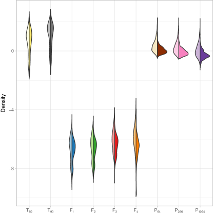
There are $374$ GRBs in the BATSE catalogue with incomplete information in one or more parameters (mainly in the four fluences $F_{1}-F_{4}$), as seen in Table 6 that enumerates the number of missing observations for in each of the nine parameters. We present in Fig. 11 a split violinplot (Hintze & Nelson, 1998) with the left side of the violin displaying the distribution of the parameters from the 1599 GRBs and the right side displaying the distribution of the 374 GRBs that are missing observations in any other parameter. The violin plots for the two duration variables $\log_{10}T_{50}$ and $\log_{10}T_{90}$ are very similar but the four peak fluxes $\log_{10}F_{1}-\log_{10}F_{4}$ generally have lower values for the missing cases. The densities of the three peak fluxes $\log_{10}P_{64}$, $\log_{10}P_{256}$ and $\log_{10}P_{1024}$ have heavier right tails for the 1599 GRBs compared to those of the 374 GRBs with incomplete observation. The 374 GRBs with missing parameter observations show a good degree of symmetry in all the three peak fluxes. Consequently, and as expected, their values also are generally lower for the observations with missing parameters than for the observations with all parameters observed.

3.2.2 Classification

In Section 3.1 we excluded these GRBs from multivariate analysis since standard MBC techniques and available software are not suited to address situations with missing variables. Here, we illustrate how we can use the clustering results of‘ Section 3.1 along with classification methods of Section 2.4 to group the GRBs with missing parameters. We first develop some methodology for this purpose.

Table 6: Number ($n_{j}$) of observations with incomplete information in each of the BATSE 4Br catalogue parameters (denoted by $X_{j}$).

$X_{j}$	$T_{50}$	$T_{90}$	$P_{64}$	$P_{256}$	$P_{1024}$	$F_{1}$	$F_{2}$	$F_{3}$	$F_{4}$
$n_{j}$	0	0	1	1	1	29	12	6	339

Corollary 1 implies that excluding the parameters that are missing for a GRB yields an observation of reduced dimensions that still has a multivariate t-distribution with parameters corresponding to the observed parameters. Therefore the classification rule of Section 2.4 can still be used with reduced $t_{\nu}$ density as per Corollary 1 taking the place of the densities $f_{i}$’s in that section. Therefore, the parameter estimates returned by $t$MMBC as per our ECM algorithm of 2.1 can be used. Specifically, the estimated $\mu_{k}$s are used, but only the parameters that are observed for the GRB under consideration are included in the calculation of the classification rule. Similarly, only the rows and columns of $\Sigma_{k}$s that correspond to the observed parameters are included in the classification rule. The estimated prior proportions $\pi_{k}$’s can be used unchanged in the classification rule calculations.

Table 7: (a) Number of missing observations in each of the nine parameters for each of the five groups. (b) group means of the nine parameters for the classified GRBs. Note that this mean is computed for a parameter only for those GRBs that did not have missing observations in that parameter for that group.

$k$	$\log T_{50}$	$\log T_{90}$	$\log F_{1}$	$\log F_{2}$	$\log F_{3}$	$\log F_{4}$	$\log P_{64}$	$\log P_{256}$	$\log P_{1024}$
1	0	0	6	6	5	131	1	1	1
2	0	0	11	4	1	38	0	0	0
3	0	0	10	1	0	22	0	0	0
4	0	0	1	1	0	125	0	0	0
5	0	0	1	0	0	23	0	0	0

(a) Number of missing observations in each of the parameters for each group

$k$	$\log T_{50}$	$\log T_{90}$	$\log F_{1}$	$\log F_{2}$	$\log F_{3}$	$\log F_{4}$	$\log P_{64}$	$\log P_{256}$	$\log P_{1024}$
1	0.68(0.05)	1.05(0.05)	-6.81(0.04)	-6.76(0.04)	-6.50(0.04)	-5.95(0.26)	-0.04(0.02)	-0.16(0.02)	-0.30(0.02)
	0.67(0.87)	1.05(0.88)	-6.82(0.55)	-6.75(0.56)	-6.44(0.58)	-5.96(0.53)	-0.07(0.23)	-0.21(0.25)	-0.34(0.232)
2	-0.76(0.11)	-0.37(0.11)	-7.92(0.07)	-7.95(0.05)	-7.34(0.04)	-6.62(0.16)	0.19(0.03)	-0.11(0.02)	-0.61(0.03)
	-0.89(0.88)	-0.55(1.06)	-8.03(0.59)	-7.91(0.44)	-7.32(0.35)	-6.53(0.75)	0.18(0.30)	-0.104(0.279)	-0.593(0.314)
3	-0.74(0.05)	-0.35(0.05)	-8.10(0.08)	-7.84(0.04)	-7.17(0.04)	-7.09(0.32)	0.18(0.04)	-0.01(0.04)	-0.44(0.04)
	-0.74(0.30)	-0.35(0.48)	-8.07(0.29)	-7.83(0.28)	-7.17(0.21)	-6.81(0.96)	0.17(0.20)	0.02(0.23)	-0.43(0.18)
4	1.23(0.04)	1.63(0.03)	-6.34(0.04)	-6.29(0.04)	-6.02(0.03)	-8.07(1.49)	0.01(0.02)	-0.07(0.02)	-0.13(0.02)
	1.26(0.55)	1.66(0.40)	-6.33(0.53)	-6.29(0.45)	-6.01(0.51)	-8.07(1.49)	-0.01(0.27)	-0.10(0.32)	-0.18(0.33)
5	0.89(0.11)	1.53(0.11)	-6.32(0.09)	-6.18(0.10)	-5.91(0.12)	-3.95(-)	0.36(0.07)	0.31(0.07)	0.18(0.07)
	0.85(0.80)	1.60(0.80)	-6.33(0.51)	-6.18(0.58)	-6.03(0.55)	-3.96(0)	0.35(0.33)	0.29(0.33)	0.15(0.35)

(b) Mean (top row) and median (bottom row) parameter values for each group. The figures in parenthesis are (top row) the standard error of the mean and the inter-quartile range (bottom row). For each group, calculations are based on the GRBs that are not missing the particular parameter for that group. “-” indicates that there was only one observed field for that parameter in that group.

Figure 11: Split violin plot of the nine observed variables where the left side of each violin is the kernel density estimate of the 1599 GRBs with complete information and the right side is the kernel density estimate of the 374 GRBs with incomplete information.

Using the above rule, we classified the 374 GRBs. Table 7 displays the number of missing parameters in each group and the descriptive statistics for each group. There were 138 GRBs classified to the long-intermediate-intermediate group, 52 GRBs to short-faint-intermediate group, 33 GRBs to short-faint-soft group, 127 GRBs to long-bright-hard group and 24 GRBs to long-intermediate-hard group. Finally, we note that our classification strategy does not have the ability to find (potentially) additional classes in the GRBs with missing parameters because we are using the classes found from clustering the 1599 GRBs in the assignment. Therefore, it would be desirable to have methodology that groups GRBs with missing and complete observations in a holistic approach. Development of such a statistical approach for tMMBC, while necessary, is however beyond the scope of this paper.

4 Conclusions

Many authors have attempted to determine the kinds of GRBs in the BATSE catalogue using various statistical techniques. While most authors have suggested that there are two kinds of GRBs, a few others have claimed this number to to be three and not two. Recently Chattopadhyay & Maitra (2017) classified 1599 GRBs using GMMBC using three original and three derived variables and found the optimal number of groups to be five. They presented carefully analyzed evidences in support of their findings. Motivated by the fact that the nine original variables might contain useful clustering information we carried out MBC using the nine original variables after checking for redundancy among them. Clustering the 1599 GRBs using $t$MMBC showed that the optimal number of homogeneous groups is five and further supports the results obtained by Chattopadhyay & Maitra (2017) providing evidence that the additional ellipsoidal groups found by them can not be subsumed inside groups with heavier tails. These groups are also more distinct than the the groups obtained in Chattopadhyay & Maitra (2017) as per the overlap measure of Maitra & Melnykov (2010). Using the classification scheme of Mukherjee et al. (1998) and Chattopadhyay & Maitra (2017) our five groups have were classified as long-intermediate-intermediate, short-faint-intermediate, short-faint-soft, long-bright-hard, and long-intermediate-hard. Further a Bayes Classifier categorized 374 GRBs having missing information in one or more of the parameters to the five groups obtained from the 1599 GRBs having complete information using $t$MMBC. 138 GRBs were classified to the long-intermediate-intermediate group, 52 GRBs to the short-faint-intermediate group, 33 GRBs to the short-faint-soft group, 127 GRBs to the long-bright-hard group and 24 GRBs to the long-intermediate-hard group.

Our article has found five ellipoidally-dispersed groups. Recent work (Almodóvar-Rivera & Maitra, 2018) on syncytial clustering when applied to the results of the analysis indicated that the number of general-shaped groups in the BATSE 4Br GRB catalog is indeed five and these five groups happen to be ellipsoidally-dispersed. Therefore, we have great confidence in our finding that there are five kinds of GRBs in the BATSE 4Br catalog.

There are a number of issues which can be looked upon as potential research problems. For one, it would be useful to incorporate and further develop clustering methods that have the ability to group observations that are complete and missing information in a holistic manner. Lithio & Maitra (2018) have, among others, redesigned the $k$-means algorithm for such scenarios but efficient methodology and software to fit $t$-mixture models with incomplete records would also be helpful. Further, use of the logarithmic transformation, while standard in GRB analysis, may obfuscate further group structure so an approach which incorporates finding the transformation within the context of clustering would be worthwhile to explore. Finally, the analysis in this paper can be extended to GRBs catalogued from sources such as the datasets from the Swift and Fermi satellites to analyse whether similar results hold for GRBs observed from these other satellites.

References

- Abramowitz & Stegun (1964) Abramowitz M., Stegun I. A., 1964, Handbook of Mathematical Functions with Formulas, Graphs, and Mathematical Tables, Ninth Dover printing, tenth GPO printing edn. Dover, New York
- Acuner & Ryde (2018) Acuner Z., Ryde F., 2018, Monthly Notices of the Royal Astronomical Society, 475, 1708
- Almodóvar-Rivera & Maitra (2018) Almodóvar-Rivera I., Maitra R., 2018, preprint, (arXiv:1805.09505)
- Andrews (1972) Andrews D. F., 1972, Biometrics, 28, 125
- Andrews & McNicholas (2012) Andrews J. L., McNicholas P. D., 2012, Statistics and Computing, 22, 1021
- Andrews & McNicholas (2015) Andrews J. L., McNicholas P. D., 2015, teigen: Model-based clustering and classification with the multivariate t-distribution
- Bernardo & Smith (1993) Bernardo J. M., Smith A. F. M., 1993, Bayesian Theory. Wiley
- Chattopadhyay & Maitra (2017) Chattopadhyay S., Maitra R., 2017, Monthly Notices of the Royal Astronomical Society, 469, 3374
- Chattopadhyay et al. (2007) Chattopadhyay T., Misra R., Chattopadhyay A. K., Naskar M., 2007, ApJ, 667, 1017
- Chen & Maitra (2011) Chen W.-C., Maitra R., 2011, Statistical Analysis and Data Mining, 4, 567
- Dempster et al. (1977) Dempster A. P., Laird N. M., Rubin D. B., 1977, Jounal of the Royal Statistical Society, Series B, 39, 1
- Dezalay et al. (1992) Dezalay J.-P., Barat C., Talon R., Syunyaev R., Terekhov O., Kuznetsov A., 1992, in Paciesas W. S., Fishman G. J., eds, American Institute of Physics Conference Series Vol. 265, American Institute of Physics Conference Series. pp 304–309
- Fraley & Raftery (1998) Fraley C., Raftery A. E., 1998, The Computer Journal, 41, 578
- Fraley & Raftery (2002a) Fraley C., Raftery A. E., 2002a, Journal of the American Statistical Association, 97, 611
- Fraley & Raftery (2002b) Fraley C., Raftery A. E., 2002b, Journal of the American Statistical Association, 97, 611
- Fraley et al. (2012) Fraley C., Raftery A. E., Murphy T. B., Scrucca L., 2012, mclust Version 4 for R: Normal Mixture Modeling for Model-Based Clustering, Classification, and Density Estimation
- Hintze & Nelson (1998) Hintze J. L., Nelson R. D., 1998, The American Statistician, 52, 181
- Horváth (1998) Horváth I., 1998, ApJ, 508, 757
- Horváth (2002) Horváth I., 2002, A&A, 392, 791
- Horváth (2009) Horváth I., 2009, Ap&SS, 323
- Horváth & Tóth (2016) Horváth I., Tóth B. G., 2016, Ap&SS, 361, 155
- Horváth et al. (2008) Horváth I., Balázs L. G., Bagoly Z., Veres P., 2008, A&A, 489, L1
- Hubert & Arabie (1985) Hubert L., Arabie P., 1985, Journal of Classification, 2, 193
- Huja, D. et al. (2009) Huja, D. Mészáros, A. Řípa, J. 2009, A&A, 504, 67
- Inselberg (1985) Inselberg A., 1985, The Visual Computer, 1, 69
- Johnson & Wichern (1988) Johnson R. A., Wichern D. W., eds, 1988, Applied Multivariate Statistical Analysis. Prentice-Hall, Inc., Upper Saddle River, NJ, USA
- Kass & Raftery (1995) Kass R. E., Raftery A. E., 1995, Journal of the American Statistical Association, 90, 773
- Khattree & Naik (2002) Khattree R., Naik D. N., 2002, Journal of Statistical Planning and Inference, 100, 411
- Kouveliotou et al. (1993) Kouveliotou C., Meegan C. A., Fishman G. J., Bhat N. P., Briggs M. S., Koshut T. M., Paciesas W. S., Pendleton G. N., 1993, ApJ, 413, L101
- Kulkarni & Desai (2017) Kulkarni S., Desai S., 2017, Ap&SS, 362, 70
- Lithio & Maitra (2018) Lithio A., Maitra R., 2018, Statistical Analysis and Data Mining – The ASA Data Science Journal
- Maitra (2001) Maitra R., 2001, Technometrics, 43, 336
- Maitra (2009) Maitra R., 2009, IEEE/ACM Transactions on Computational Biology and Bioinformatics, 6, 144
- Maitra (2010) Maitra R., 2010, NeuroImage, 50, 124
- Maitra & Melnykov (2010) Maitra R., Melnykov V., 2010, Journal of Computational and Graphical Statistics, 19, 354
- Maitra et al. (2012) Maitra R., Melnykov V., Lahiri S., 2012, Journal of the American Statistical Association, 107, 378
- Mazets et al. (1981) Mazets E. P., et al., 1981, Ap&SS, 80, 3
- McLachlan & Krishnan (2008) McLachlan G., Krishnan T., 2008, The EM Algorithm and Extensions, second edn. Wiley, New York, doi:10.2307/2534032
- McLachlan & Peel (1998) McLachlan G. J., Peel D., 1998, in Amin A., Dori D., Pudil P., Freeman H., eds, Advances in Pattern Recognition: Joint IAPR International Workshops SSPR’98 and SPR’98 Sydney, Australia, August 11–13, 1998 Proceedings. Springer Berlin Heidelberg, Berlin, Heidelberg, pp 658–666, doi:10.1007/BFb0033290
- McLachlan & Peel (2000) McLachlan G., Peel D., 2000, Finite Mixture Models. John Wiley and Sons, Inc., New York, doi:10.1002/0471721182
- Melnykov & Maitra (2010) Melnykov V., Maitra R., 2010, Statist. Surv., 4, 80
- Melnykov & Maitra (2011) Melnykov V., Maitra R., 2011, Journal of Machine Learning Research, 12, 69
- Melnykov et al. (2012) Melnykov V., Chen W.-C., Maitra R., 2012, Journal of Statistical Software, 51, 1
- Meng & Rubin (1993) Meng X.-L., Rubin D. B., 1993, Biometrika, 80, 267
- Meng & Van Dyk (1997) Meng X.-L., Van Dyk D., 1997, Journal of the Royal Statistical Society: Series B (Statistical Methodology), 59, 511
- Mukherjee et al. (1998) Mukherjee S., Feigelson E. D., Jogesh Babu G., Murtagh F., Fraley C., Raftery A., 1998, ApJ, 508, 314
- Nakar (2007) Nakar E., 2007, Physics Reports, 442, 166
- Norris et al. (1984) Norris J. P., Cline T. L., Desai U. D., Teegarden B. J., 1984, Nature, 308, 434
- Paczyński (1998) Paczyński B., 1998, ApJ, 494, L45
- Pendleton et al. (1997) Pendleton G. N., et al., 1997, The Astrophysical Journal, 489, 175
- R Core Team (2017) R Core Team 2017, R: A Language and Environment for Statistical Computing. R Foundation for Statistical Computing, Vienna, Austria, https://www.R-project.org/
- Raftery & Dean (2006) Raftery A. E., Dean N., 2006, Journal of the American Statistical Association, 101, 168
- Rand (1971) Rand W. M., 1971, Journal of the American Statistical Association, 66, 846
- Schwarz (1978) Schwarz G., 1978, Ann. Statist., 6, 461
- Tarnopolski (2015) Tarnopolski M., 2015, A&A, 581, A29
- Wegman (1990) Wegman E., 1990, Journal of the American Statistical Association, 85, 664
- Woosley & Bloom (2006) Woosley S., Bloom J., 2006, ARA&A, 44, 507
- Zhang et al. (2016) Zhang Z.-B., Yang E.-B., Choi C.-S., Chang H.-Y., 2016, MNRAS, 462, 3243
- Zitouni et al. (2015) Zitouni H., Guessoum N., Azzam W. J., Mochkovitch R., 2015, Ap&SS, 357, 7
- Řípa et al. (2009) Řípa J., Mészáros A., Wigger C., Huja D., Hudec R., Hajdas W., 2009, A&A, 498, 399