Derivation of a hydrodynamic theory for mesoscale dynamics in microswimmer suspensions

Abstract

In this paper we systematically derive a fourth-order continuum theory capable of reproducing mesoscale turbulence in a three-dimensional suspension of microswimmers. We start from overdamped Langevin equations for a generic microscopic model (pushers or pullers), which include hydrodynamic interactions on both, small length scales (polar alignment of neighboring swimmers) and large length scales, where the solvent flow interacts with the order parameter field. The flow field is determined via the Stokes equation supplemented by an ansatz for the stress tensor. In addition to hydrodynamic interactions, we allow for nematic pair interactions stemming from excluded-volume effects. The results here substantially extend and generalize earlier findings [Phys. Rev. E 94, 020601(R) (2016)], in which we derived a two-dimensional hydrodynamic theory. From the corresponding mean-field Fokker-Planck equation combined with a self-consistent closure scheme, we derive nonlinear field equations for the polar and the nematic order parameter, involving gradient terms of up to fourth order. We find that the effective microswimmer dynamics depends on the coupling between solvent flow and orientational order. For very weak coupling corresponding to a high viscosity of the suspension, the dynamics of mesoscale turbulence can be described by a simplified model containing only an effective microswimmer velocity.

I Introduction

Self-organized structures of actively driven constituents are fascinating non-equilibrium phenomena which are fundamental for the development of life. Due to the large number of constituents in such systems, continuum theories provide a useful tool to describe and analyse how the microscopic details of system constituents and the interactions between them give rise to large scale collective structures observed in experiments. These range from large scale vortex structures Sumino et al. (2012); Schaller et al. (2010); Nishiguchi and Sano (2015); Rabani et al. (2013), dynamical clustering Buttinoni et al. (2013); Peruani et al. (2012), giant number fluctuations Simha and Ramaswamy (2002); Zhang et al. (2010) and actively driven phase separations Schwarz-Linek et al. (2012); Wittkowski et al. (2014); Buttinoni et al. (2013); Speck et al. (2014) to bacterial turbulence Dombrowski et al. (2004); Bratanov et al. (2015); Oza et al. (2016); Heidenreich et al. (2014). For recent reviews on active matter, see Ramaswamy (2010); Romanczuk et al. (2012); Marchetti et al. (2013); Elgeti et al. (2015); Bechinger et al. (2016); Zöttl and Stark (2016); Menzel (2015). Even if the interactions between living microswimmers are complex and characterized by many details, the observed collective patterns often show a generalized behavior. Therefore, the continuum description of such systems uses symmetry arguments and extra terms for the activity driving the system out of equilibrium.

Due to the fascinating nature of collective phenomena in active systems, many efforts have been made to find general models for large collections of active moving particles. The models proposed in recent years range from kinetic and continuum theories based on microscopic models to purely phenomenological approaches Peshkov et al. (2012a, b); Baskaran and Marchetti (2008); Ahmadi et al. (2005); Grossmann et al. (2012); Menzel et al. (2016); Saintillan and Shelley (2008, 2009); Toner and Tu (1998); Großmann et al. (2014, 2015). In most of the systems the individual microswimmer exhibits an axis defining a direction that breaks the rotational symmetry. The density distribution of a large collection of microswimmers then depends on the position and the orientation of the individuals. Depending on the symmetry of the distribution, the system can either exhibit polar (e.g., in polar active fluids) or nematic order (e.g., for active nematics). Examples for nematically ordered matter are microtubuli-kinesin mixtures Sanchez et al. (2012) or swimming bacteria in a lyotropic liquid crystal Zhou et al. (2014); Genkin et al. (2017). Due to the symmetry of the orientational distribution, active nematics are usually described by a second rank tensor (nematic order parameter) coupled to a vector field describing the fluid in which the microswimmers are swimming Ahmadi et al. (2005); Hemingway et al. (2016); Doostmohammadi et al. (2016). In this paper we consider an active fluid consisting of polar moving active particles like bacterial suspensions Saintillan and Shelley (2008, 2009); Toner and Tu (1998).

In a recent approach, a phenomenological model for the collective dynamics of B. subtilis suspensions has been proposed Wensink et al. (2012). The idea was to extend the seminal Toner-Tu equation Toner and Tu (1998) introduced solely on symmetry arguments as the continuum counterpart of the Vicsek model Vicsek et al. (1995) for moving active particles (e.g., to describe flocks of flying birds). The Toner-Tu equation exhibits polar symmetry and is able to describe the transition from a disordered state to an ordered (polar) state that corresponds to the collective movement of active individuals. For constant density (as expected in dense suspensions) the Toner-Tu equation has two homogeneous fixed points, but shows no heterogeneous dynamics as observed for bacterial suspensions. The reason is a positive parameter of the Laplacian that damps excited spatial modes. By allowing negative values, excited modes increase and the homogeneous state becomes unstable. Such a theory then has to be extended to higher (fourth) order derivatives for stability reasons.

Such higher order derivative equations have been frequently used in the theory of pattern formation. A simple theory modeling the formation of patterns at a certain length scale is the Swift-Hohenberg equation. This scalar fourth order theory exhibits a Turing instability and shows, e.g., stripes, labyrinth or hexagonal patterns in two dimensions. A combination of the characteristic features of the Swift-Hohenberg with the Toner-Tu equations yields a surprisingly rich phenomenological description of bacterial turbulence. In particular, a fourth order field theory for the divergence-free collective velocity ${\bf w}$, i.e.,

$$\left(\partial_{t}+\lambda_{0}{\bf w}\cdot\nabla\right){\bf w}= -\nabla p+\lambda_{1}\nabla|{\bf w}|^{2}-\alpha{\bf w}-\beta|{\bf w}|^{2}{\bf w}$$ (1)

$$+\Gamma_{2}\nabla^{2}{\bf w}+\Gamma_{4}\nabla^{4}{\bf w},$$

is able to model the main features of mesoscale turbulence Dunkel et al. (2013a, b); Wensink et al. (2012); Bratanov et al. (2015); Zhang et al. (2009). The ratio of the phenomenological parameters $\Gamma_{2}$ and $\Gamma_{4}$ determines the characteristic scale, the typical vortex size $\Lambda$, in bacterial suspensions, viz., $\Lambda=2\pi\sqrt{2\Gamma_{4}/\Gamma_{2}}$. By adjusting these parameters and the parameter $\lambda_{0}$ to experimental data, the dynamics of the observed bacterial suspensions can be described quantitatively.

The phenomenological model describes the dynamics of an effective velocity and does not distinguish between orientation and the dynamics of the surrounding fluid. However, recent experiments of B. subtilis suspensions and simulations of Wioland, Lushi and coworkers have shown the importance of the solvent hydrodynamics for the collective dynamics Lushi et al. (2014). In an earlier rapid communication we introduced a two-dimensional field theory including the solvent flow dynamics Heidenreich et al. (2016).

The purpose of the present article is to derive a continuum model from a generic microscopic model with polar and nematic alignment interactions combined with an effective treatment of hydrodynamic interactions with the ambient fluid for two and three spatial dimensions. In particular, the theory resulting in this paper is capable to describe the dynamics of three-dimensional microswimmer suspensions.

The next section introduces our microscopic model by a set of overdamped Langevin equations. We then derive the related Fokker-Planck equation and by projection onto the orientational moments we obtain an infinite hierarchy of moment equations. Using appropriate closure conditions to truncate the hierarchy finally yields the continuum equations.

In our previous publication Heidenreich et al. (2016) we sketched the derivation of a 2D field theory from a microscopic model. The focus was to show that the typical length scale in mesoscale turbulence depends on details of the microswimmers themselves. In this paper we give an elaborate derivation of a 2D and 3D field theory from a microscopic model that in addition includes nematic interactions. We show that the microscopic parameters have a strong influence on the collective dynamics of mesoscale turbulence. In particular, we identify a coupling parameter characterizing the flow’s response to the activity. In the limit of very weak coupling, the system can be adequately described by the dynamics of only one order parameter and we recover the phenomenological Eq. (1) for the effective microswimmer velocity. Finally, we present 3D simulations focusing on the limit of weak coupling.

II Microscopic theory

II.1 Microswimmer model

Active suspensions are comprised of millions of microswimmers moving in a Newtonian solvent fluid such as water. The swimming mechanism is based on non-reciprocal movements in time, which cause a flow of the surrounding fluid. The characteristics of the flow depend on the type of swimmer considered (e.g., bacterial swimmer, algae cell or chemically driven nano-rod). However, at large distances and on time scales beyond a typical stroke period, the flow can often be approximately described by a moving force dipole resulting from two close point forces ${\bf F}$ with opposite directions. One distinguishes between pushers and pullers. A pusher particle (such as, e.g., Escherichia Coli bacteria Drescher et al. (2011)) pumps the solvent fluid from its sides towards the rear and the front, as described by two forces pointing away from one another. In contrast, for pullers (e.g., Chlamydomonas Reinhardtii) the forces point towards each other. An illustration of these situations is given in Fig. 1 which also introduces our particle model.

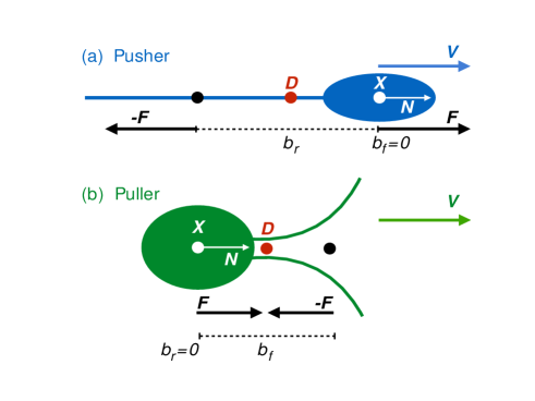
Figure 1: (Color online) Schematic of a model microswimmer of type ”pusher” (a) or ”puller” (b). The center of hydrodynamic stress (X) is located in front (pusher) or behind (puller) the location of the force dipole (D). The distances between X and the acting forces is given by $b_{f}$ and $b_{r}$, respectively. The orientation of the swimmer’s long axis, ${\bf N}$ defines the direction of the velocity, ${\bf v}$.

Each microswimmer is represented by a cylindrical rod moving along the direction of its long axis, described by the vector ${\bf N}$. The front force, ${\bf F}_{f}=f_{0}{\bf N}$ (with $f_{0}$ being positive or negative for a pusher or puller, respectively) acts at position ${\bf X}_{f}={\bf X}+b_{f}{\bf N}$, where $b_{f}>0$ and ${\bf X}$ is the center of hydrodynamic stress, i.e., the point where the hydrodynamic net torque on a rigid body vanishes Happel and Brenner (2012). We will later use ${\bf X}$ to describe the position of the swimmer in space. The rear force, ${\bf F}_{r}=-f_{0}{\bf N}=-{\bf F}_{f}$ acts at position ${\bf X}_{r}={\bf X}-b_{r}{\bf N}$ (with $b_{r}>0$). The entire rod is then moving with velocity ${\bf v}=v_{0}{\bf N}$ (with $v_{0}$ being the self-propulsion velocity) similarly to self-propelled rod models Ginelli et al. (2010); Yang et al. (2010); Wensink and Löwen (2008); Peruani et al. (2006); Großmann et al. (2016).

With these assumptions, the force density in the solvent generated by a single microswimmer is given by

$${\bf f}({\bf x},t) = {\bf F}_{r}\delta({\bf x}-{\bf X}_{r})+{\bf F}_{f}\delta({\bf x}-{\bf X}_{f}).$$ (2)

We will later make use of this expression to calculate the active stress tensor ${\boldsymbol{\sigma}}^{\mathrm{a}}$ resulting from the forcing of the fluid by a collection of swimmers. The active stress is an important ingredient of the Stokes equation (valid at low Reynolds numbers) for the fluid velocity ${\bf u}$.

II.2 Microscopic equations of motion

We now consider an ensemble of $\sigma=1,\ldots,S$ identical microswimmers of the type introduced in Fig. 1. The aim in this section is to formulate equations of motion incorporating, on the one hand, direct conservative (e.g., repulsive) interactions between the swimmers, and, on the other hand, indirect (hydrodynamic) interactions induced by the solvent flow. Following our earlier paper Heidenreich et al. (2016) we take into account these interactions on a coarse-grained level of description. Various studies (see, e.g., Refs. Najafi and Golestanian (2004); Pooley et al. (2007); Avron et al. (2005)) have proposed a microscopic modeling of the interaction between swimmer and solvent flow. However, due to the detailed nature of these models they are not convenient for the derivation of a continuum theory targeting the collective behavior of a large number of microswimmers.

Within our coarse-grained description, the interactions are grouped into two contributions, see Fig. 2 for an illustration. The first contribution comprises all short-range effects. Specifically, it summarizes the repulsive (rod-rod) pair interactions as well as the near-field hydrodynamic interactions between swimmers $\nu$ and $\mu$ by an anisotropic pair potential (to be specified below), which couples the orientations ${\bf N}^{\nu}$ and ${\bf N}^{\mu}$ at distances up to a fixed range. The second contribution accounts for far-field hydrodynamic effects; these are incorporated by terms which couple the orientation ${\bf N}^{\nu}$ with the (averaged) solvent flow ${\bf u}$. The latter is a collective quantity in the sense that it involves the stroke-averaged far fields generated by all the individuals (see Sec. III.2).

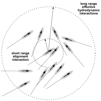
Figure 2: Schematic of the two types of interactions incorporated in our model: short-range interactions favoring alignment (inner circle), and long range hydrodynamic interactions (outer ring).

II.2.1 Pair interactions

In the following we first specify the short-range pair interactions. Experimentally one observes that bacteria and other microswimmers locally tend to swim along the same direction Zhang et al. (2010). Within our description this corresponds to an activity-driven polar alignment of the orientation vectors ${\bf N}^{\nu}$, ${\bf N}^{\mu}$ of neighboring particles. Note that this is a simplified model describing only the aligning effect of near-field hydrodynamic interactions and neglecting any higher order tensorial components. For a classification of active systems see Marchetti et al. (2013). Specifically, we use the ansatz

$$\Phi^{\mathrm{act}}\left({\bf N}^{\nu},{\bf N}^{\mu},r_{\mu\nu}\right) = -\frac{\gamma_{0}v_{0}}{2}{\bf N}^{\nu}\cdot{\bf N}^{\mu}\,\Theta(\epsilon_{a}-r_{\mu\nu}),$$ (3)

where $\gamma_{0}>0$ is the magnitude of the interaction, $r_{\mu\nu}=|\boldsymbol{X}^{\mu}-\boldsymbol{X}^{\nu}|$ is the particle distance, and $\Theta(x)$ is the theta-function (with $\Theta(x)=1$, $x\geq 0$, and zero otherwise). The latter expresses the fact that the range of the polar interaction is restricted to distances smaller than $\epsilon_{a}$. The appearance of the self-propulsion velocity $v_{0}$ in the prefactor reflects the ”active” nature of this interaction. However, even at $v_{0}=0$ (dead microswimmer) there is a steric interaction between the bodies. On a mean-field (Maier-Saupe) level, these lead to a passive nematic potential Maier and Saupe (1958, 1959, 1960)

$$\Phi^{\mathrm{pass}}\left({\bf N}^{\nu},{\bf N}^{\mu},r_{\mu\nu}\right) = -\frac{\gamma_{1}}{4}\left({\bf N}^{\nu}\cdot{\bf N}^{\mu}\right)^{2}\,\Theta(\epsilon_{p}-r_{\mu\nu}),$$

where $\gamma_{1}>0$. Both potentials are of square-well type, i.e., they are independent of the distance within the range of the respective interaction ranges. This choice reflects our focus on reorientation effects; in fact, the impact of direct steric collisions on the translational motion is neglected in our model. Realistically, the ranges $\epsilon_{a}$, $\epsilon_{p}$ should be comparable to the microswimmers’ length. For convenience we choose $\epsilon_{a}=\epsilon_{p}=\epsilon$. The total potential function stemming from short-range interactions is then given by the pair sums of Eqs. (3) and (II.2.1),

$$\Phi=\sum_{\mu,\nu}\left(\Phi^{\mathrm{act}}\left({\bf N}^{\nu},{\bf N}^{\mu},r_{\mu\nu}\right)+\Phi^{\mathrm{pass}}\left({\bf N}^{\nu},{\bf N}^{\mu},r_{\mu\nu}\right)\right).$$

Our approach of including the far-field hydrodynamic effects will be specified in the next paragraphs.

II.2.2 Langevin equations

To model the (overdamped) translational and orientational motion of the ensemble of microswimmers we employ the Langevin equations

$$\frac{d}{dt}{\bf X}^{\sigma}(t) = v_{0}{\bf N}^{\sigma}(t)+{\bf u}({\bf X}^{\sigma},t)+\sqrt{2D}\;\boldsymbol{\xi}^{\sigma}(t),$$ (6a)

$$\frac{d}{dt}{\bf N}^{\sigma}(t) = {\boldsymbol{\Omega}({\bf X}^{\sigma},t)\cdot{\bf N}^{\sigma}}(t)+{\boldsymbol{\Pi}}({\bf N}^{\sigma})\cdot\left[a_{0}\boldsymbol{\Sigma}({\bf X}^{\sigma},t)\cdot{\bf N}^{\sigma}(t)\right.$$ (6b)

$$\left.-{\nabla}_{{\bf N}^{\sigma}}\Phi({\bf N})+\tau^{-1/2}\;{\boldsymbol{\eta}}^{\sigma}(t)\right],$$

where the random functions $\boldsymbol{\xi}^{\sigma}(t)$ and $\boldsymbol{\eta}^{\sigma}(t)$ denote Gaussian white noise mimicking diffusion effects in the translational and orientational motion (we neglect shape-induced effects on the noise). The translational dynamics (6a) is determined by the self-propulsion (of magnitude $v_{0}$) in direction of ${\bf N}$, as well as by the advection ${\bf u}$. Here, $\bf u$ is the average flow field to be calculated via the averaged Stokes equation (see Eq. (8) below). Thus, we adopt the mean-field-like assumption that the fluctuating field ${\bf u}$ can be replaced by its average.

The orientational dynamics (6b) is determined, first, by the short-range anisotropic interactions $\Phi$ defined in Eq. (II.2.1). Second, Eq. (6b) takes into account the far-field hydrodynamic effects via the coupling terms involving the vorticity ${\boldsymbol{\Omega}}=\frac{1}{2}\left[\left(\nabla{\bf u}\right)^{\top}-\nabla\boldsymbol{u}\right]$, which describes the torque of the solvent flow, and the strain rate tensor ${\boldsymbol{\Sigma}}=\frac{1}{2}\left[\left(\nabla{\bf u}\right)^{\top}+\nabla\boldsymbol{u}\right]$ describing the effect of a flow gradient. Finally, there appears the projector $\boldsymbol{\Pi}({\bf N}^{\sigma})={\bf I}-{\bf N}^{\sigma}{\bf N}^{\sigma}$ (with ${\bf I}$ being the unit matrix), which conserves the length of the orientation vector ${\bf N}^{\sigma}$. The entire Eq. (6b) is interpreted as a Stratonovich stochastic differential equation with rotational relaxation time $\tau$.

We note that the coupling terms $\boldsymbol{\Omega}\cdot{\bf N}^{\sigma}+\boldsymbol{\Pi}\cdot a_{0}\boldsymbol{\Sigma}\cdot{\bf N}^{\sigma}$ in Eq. (6b) remind of Jeffrey’s theory for the oscillatory tumbling motion of elongated passive particles Jeffery (1922); Hinch and Leal (1979); Pedley and Kessler (1992). In that theory, the magnitude of the coupling depends on the aspect (length-to-width) ratio $r$ of the particles via the shape parameter

$$a_{0}=(r^{2}-1)/(r^{2}+1).$$ (7)

Because the Jeffrey equation has been proposed for passive rods, the validity of Eq. (7) for active particles is not immediately clear. Indeed, Rafaï and co-workers Rafaï et al. (2010) have experimentally shown that the Jeffrey tumbling period Jeffery (1922) of Chlamydomonas algae depend on their swimming conditions. Further, it has been found Jibuti et al. (2017) that the tumbling period in a shear flow of living cells can be larger or lower than the tumbling period of the corresponding dead cells. Nevertheless, one may expect a dependence of the shape parameter $a_{0}$ on the swimmer size $\ell$ also for active particles, thus we stick to Eq. (7).

II.3 Far-field hydrodynamic interactions

We distinguish between near-field and far-field hydrodynamic interactions, the former already specified by the effective polar interaction potential above (see Eq. 3). The latter are taken into account by the coupling of Eqs. (6a) and (6b) to the average flow field ${\bf u}$.

II.3.1 Stokes equation

In the limit of low Reynolds numbers, ${\bf u}$ is determined by the averaged Stokes equation

$$0=-{\nabla}p+\mu^{*}\nabla^{2}{\bf u}+\nabla\cdot\langle{\boldsymbol{\sigma}}\rangle,$$ (8)

combined with the incompressibility condition (appropriate at large densities)

$$0=\nabla\cdot{\bf u}.$$ (9)

In Eq. (8), $p$ is the hydrodynamic pressure, $\langle{\boldsymbol{\sigma}}\rangle$ is the averaged stress tensor (to be discussed in the next paragraph), and $\mu^{*}$ is the effective bulk viscosity. The latter includes contributions from the solvent as well as from the embedded colloids or bacteria. As an approximation, we here employ the Batchelor-Einstein relation for passive, spherical particles Hinch (2010); Einstein (1906); Batchelor (1974). The latter is given as $\mu^{*}=\mu_{0}(1+k_{1}c+k_{3}c^{2})$ where $\mu_{0}$ is the ”bare” solvent viscosity and $c=V_{0}n$ is the volume fraction (with $n$ being the number of particles per unit volume $V_{0}=4\pi a^{3}/3$ for a sphere of radius $a$). The coefficients are $k_{1}=5/2$ in three dimensions Hinch (2010); Einstein (1906) and $k_{1}=2$ in two dimensions Haines et al. (2008), respectively. The second order coefficient can be similarly calculated for passive spherical colloidal particles Hinch (2010). For active microswimmer suspensions there is an additional term $k_{2}$ with a negative sign that emerges within the derivation given later Heidenreich et al. (2016).

Using the values for the passive case for $k_{1}$ and $k_{3}$ the effective bulk viscosity of Chlamydomonas Reinhardtii (puller) suspensions is well described Rafaï et al. (2010); Heidenreich et al. (2016). On the other hand for B. subtilis or Escherichia Coli (pusher) suspensions the value of $k_{3}$ has to be fitted to be in agreement with experimental observations Heidenreich et al. (2016).

An alternative to the Batchelor-Einstein relation is the Krieger-Dougherty equation valid for dense suspensions Krieger and Dougherty (1959), assuming a different functional form of the effective viscosity in terms of the volume fraction. In the scaling we propose later, the explicit form of the effective viscosity does not enter. In this work we thus refrain from a detailed discussion on the topic.

The Stokes equation (8) is formulated in three spatial dimensions, and this is the situation for which we later present numerical results. Likewise, we assume that the orientation vectors ${\bf N}^{\sigma}$ can have all directions on the unit sphere. However, the theory may also be adapted for a quasi-two dimensional system where one spatial dimension is very small compared to the others (thin film); this is achieved by integrating over the small dimension. Depending on boundary conditions the integration procedure may introduce some extra boundary terms, such as the Brinkmann equation for no slip conditions Brinkmann (1949).

II.3.2 Stress tensor

We now consider in more detail the stress tensor $\boldsymbol{\sigma}$, whose average appears in the Stokes equation (8). This ensures that the properties of the interacting microswimmer suspension are fed back into the flow field $\bf u$. In the present system, $\langle{\boldsymbol{\sigma}}\rangle$ consists of an active (a) and passive (p) contribution, $\langle{\boldsymbol{\sigma}}\rangle=\langle{\boldsymbol{\sigma}}^{\mathrm{a}}\rangle+\langle{\boldsymbol{\sigma}}^{\mathrm{p}}\rangle$. Here, we discuss first the microscopic, non-averaged stress tensor (the averaging will be done later in Sec. III.2.2).

The active part ${\boldsymbol{\sigma}}^{\mathrm{a}}$ is determined by forces exerted by the microswimmers onto the solvent fluid. Specifically, one has

$$\nabla\cdot{\boldsymbol{\sigma}}^{\mathrm{a}}={\bf f},$$ (10)

where ${\bf f}$ is the force density related to the $\sigma=1,\ldots,S$ force dipoles. From Eq. (2) we find that each particle $\sigma$ gives a contribution

$${\bf f}^{\sigma}({\bf x},t) = {\bf F}^{\sigma}_{r}\delta({\bf x}-{\bf X}^{\sigma}_{r})+{\bf F}^{\sigma}_{f}\delta({\bf x}-{\bf X}^{\sigma}_{f})$$ (11)

$$= -f_{0}\boldsymbol{N}^{\sigma}\left[\delta({\bf x}-{\bf X}^{\sigma}+b_{r}{\bf N}^{\sigma})\right.$$

$$\left.-\delta({\bf x}-{\bf X}^{\sigma}-b_{f}{\bf N}^{\sigma})\right].$$

where we have used that ${\bf F}^{\sigma}_{r}=-{\bf F}^{\sigma}_{f}=-f_{0}{\bf N}$, as well as the corresponding expressions for ${\bf X}_{r}$ and ${\bf X}_{f}^{\sigma}$ (see Fig. 1).

Following earlier studies Simha and Ramaswamy (2002); Hatwalne et al. (2004), we expand the force density in a Taylor series for small lengths $b_{r}$ and $b_{f}$ up to fourth order, analogous to a multipole expansion Baskaran and Marchetti (2009); Spagnolie and Lauga (2012), yielding

$${\bf f}^{\sigma}\approx-f_{0}\bf N^{\sigma} \biggl{[}(b_{r}+b_{f}){\bf N}^{\sigma}\cdot\nabla+\frac{(b_{r}^{2}-b_{f}^{2})}{2!}{\bf N}^{\sigma}{\bf N}^{\sigma}:\nabla\nabla$$ (12)

$$+\frac{(b_{r}^{3}+b_{f}^{3})}{3!}{\bf N}^{\sigma}{\bf N}^{\sigma}{\bf N}^{\sigma}:\cdot\nabla\nabla\nabla$$

$$+\frac{(b_{r}^{4}-b_{f}^{4})}{4!}{\bf N}^{\sigma}{\bf N}^{\sigma}{\bf N}^{\sigma}{\bf N}^{\sigma}::\nabla\nabla\nabla\nabla$$

$$+\dots\biggr{]}\,\delta^{\sigma},$$

where we introduced the abbreviation $\delta^{\sigma}=\delta({\bf x}-{\bf X}^{\sigma})$. Using ${\bf f}^{\sigma}=\nabla\cdot\boldsymbol{\sigma}^{\mathrm{a}}_{\sigma},$ where $\boldsymbol{\sigma}^{\mathrm{a}}_{\sigma}$ is the active stress related to particle $\sigma$, and performing a sum over all particles we find that the total active stress is given (up to an irrelevant constant) by

$${\boldsymbol{\sigma}^{\mathrm{a}}}({\bf x},t) \approx -f_{0}\biggl{[}\zeta_{1}\sum_{\sigma}{\bf N}^{\sigma}{\bf N}^{\sigma}\delta^{\sigma}+$$

$$\qquad\;\zeta_{2}\;\nabla\cdot\sum_{\sigma}{\bf N}^{\sigma}{\bf N}^{\sigma}{\bf N}^{\sigma}\delta^{\sigma}+$$

$$\qquad\;\zeta_{3}\;{\nabla}{\nabla}:\sum_{\sigma}{\bf N}^{\sigma}{\bf N}^{\sigma}{\bf N}^{\sigma}{\bf N}^{\sigma}\delta^{\sigma}+\,$$

$$\qquad\;\zeta_{4}\;\nabla\nabla\nabla:\cdot\sum_{\sigma}{\bf N}^{\sigma}{\bf N}^{\sigma}{\bf N}^{\sigma}{\bf N}^{\sigma}{\bf N}^{\sigma}\delta^{\sigma}\biggr{]},$$

where we have truncated the expansion (12) after the fifth-order term in ${\bf N}^{\sigma}$. The coefficients of the lower-order terms are given by

$$\zeta_{1} = b_{f}+b_{r}\;,\qquad\;\;\;\;\;\;\;\zeta_{2}=\frac{1}{2}(b_{r}^{2}-b_{f}^{2}),$$ (14a)

$$\zeta_{3} = \frac{1}{3!}(b_{r}^{3}+b_{f}^{3})\;,\qquad\zeta_{4}=\frac{1}{4!}(b_{r}^{4}-b_{f}^{4}).$$ (14b)

The passive stress, $\boldsymbol{\sigma}^{\mathrm{p}}$, is determined by the relation Dhont and Briels (2002),

$$\nabla\cdot\boldsymbol{\sigma}^{\mathrm{p}}=-\sum_{\sigma}\bigg{\langle}\int_{\partial V_{j}}dS\delta(r-r^{\prime}){\bf f}^{h}(r^{\prime})\bigg{\rangle},$$ (15)

where ${\bf f}^{h}(r^{\prime})$ is the force per unit area that the solvent exerts on the surface element, and $\partial V_{j}$ is the surface area of the rod.

To summarize, our microscopic model is defined by the (overdamped) Langevin equations (6a) and (6b) for the positions ${\bf X}^{\sigma}$ and orientations ${\bf N}^{\sigma}$, respectively, combined with the Stokes Eq. (8) for the flow field ${\bf u}$. The latter includes the active and passive stress from the microswimmers according to Eqs. (II.3.2) and Eq. (15).

Similar equations of motions have been derived on the basis of the slender body theory by Shelley and Saintillan Saintillan and Shelley (2008, 2009). The major difference to their work concerns the form of alignment interactions, as well as the fact that we consider higher order contributions to the active stress.

III Continuum theory

Starting from the microscopic theory presented in Sec. II we now derive continuum equations for suitable order parameter fields describing the dynamics on the mesoscale. To this end, we first set up the Fokker-Planck (FP) equation (Sec. III.1) corresponding to the Langevin equations (6a) and (6b). The FP equation then generates order parameter equations by projection. In the second step, we combine these order parameter equations with a suitably rewritten equation for the flow field (Sec. III.2).

III.1 Fokker-Planck equation

III.1.1 Probability densities and order parameters

We consider the dynamics of the one-particle probability density function

$$\mathcal{P}({\bf x},{\bf n},t)=\frac{1}{S}\sum_{\sigma=1}^{S}\bigg{\langle}\delta({\bf x}-{\bf X}^{\sigma}(t))\,\delta({\bf n}-{\bf N}^{\sigma}(t))\bigg{\rangle},\quad$$ (16)

where $\langle\,\cdot\,\rangle$ denotes an average with respect to the Gaussian white noise processes as well as an ensemble average. Based on $\mathcal{P}({\bf x},{\bf n},t)$, we can define the marginal position density $\mathcal{P}({\bf x},t)$ and the local concentration field $\rho({\bf x},t)$ via

$$\rho({\bf x},t) = S\,\mathcal{P}({\bf x},t)=S\int d{\bf n}\;\mathcal{P}({\bf x},{\bf n},t).$$ (17)

From this we obtain the (conditional) orientational density

$$\mathcal{P}({\bf n},t|{\bf x},t)=\frac{\mathcal{P}({\bf x},{\bf n},t)}{\mathcal{P}({\bf x},t)}=\frac{S\mathcal{P}({\bf x},{\bf n},t)}{\rho({\bf x},t)},$$ (18)

which describes the probability that a particle has orientation ${\bf n}$ given that it is located at position ${\bf x}$.

With $\mathcal{P}({\bf x},{\bf n},t)$ or $\mathcal{P}({\bf n},t|{\bf x},t)$ we can now define the moments of the orientation ${\bf n}$. Up to third order, the moments are given as

$$\overline{{\bf n}}({\bf x},t) \equiv \int d{\bf n}\;\mathcal{P}({\bf n},t|{\bf x},t)\;{\bf n}\quad\;$$ (19a)

$$= \frac{S}{\rho}\int d{\bf n}\;\mathcal{P}({\bf x},{\bf n},t)\;{\bf n},$$

$$\overline{{\bf n}{\bf n}}({\bf x},t) \equiv \int d{\bf n}\;\mathcal{P}({\bf n},t|{\bf x},t)\;{\bf n}{\bf n}\;\;$$ (19b)

$$= \frac{S}{\rho}\int d{\bf n}\;\mathcal{P}({\bf x},{\bf n},t)\;{\bf n}{\bf n},$$

$$\overline{{\bf n}{\bf n}{\bf n}}({\bf x},t) \equiv \int d{\bf n}\;\mathcal{P}({\bf n},t|{\bf x},t)\;{\bf n}{\bf n}{\bf n}$$ (19c)

$$= \frac{S}{\rho}\int d{\bf n}\;\mathcal{P}({\bf x},{\bf n},t)\;{\bf n}{\bf n}{\bf n}.$$

From the above definitions it follows that the moments may be considered as expectation values (averages) over the fluctuating microscopic degrees of freedom. These expectation values directly lead to the definition of the two key order parameters of our system, that is, the polarization measuring the net orientation

$${\bf P}({\bf x},t)\equiv\overline{{\bf n}}({\bf x},t)$$ (20)

and the ${\bf Q}$-tensor measuring nematic order

$${\bf Q}({\bf x},t)\equiv(\overline{{\bf n}{\bf n}})^{\text{ST}}({\bf x},t)=\overline{{\bf n}{\bf n}}({\bf x},t)-\frac{{\bf I}}{d}.$$ (21)

In Eq. (21), the notation $(\ldots)^{\text{ST}}$ denotes the symmetric traceless part of a tensor, and $d$ is the spatial dimension. For $d=2,3$, the explicit expressions for the symmetric traceless tensors in terms of the full tensors are given by

$$(\overline{n_{i}n_{j}})^{\text{ST}}({\bf x},t) = \overline{n_{i}n_{j}}-\frac{1}{d}\delta_{ij},$$ (22a)

$$(\overline{n_{i}n_{j}n_{k}})^{\text{ST}}({\bf x},t) = \overline{n_{i}n_{j}n_{k}}-\frac{3!}{2d+4}(\delta_{ij}\overline{n_{k}})^{\text{SY}},$$

$$(\overline{n_{i}n_{j}n_{k}n_{l}})^{\text{ST}}({\bf x},t) = \overline{n_{i}n_{j}n_{k}n_{l}}-\frac{4!}{4d+16}(\delta_{ij}\overline{n_{k}n_{l}})^{\text{SY}}$$ (22c)

$$+\frac{4!}{88d+16}(\delta_{ij}\delta_{kl})^{\text{SY}},$$

$$(\overline{n_{i}n_{j}n_{k}n_{l}n_{m}})^{\text{ST}}({\bf x},t) = \overline{n_{i}n_{j}n_{k}n_{l}n_{m}}$$

$$-\frac{5!}{12d+72}(\delta_{ij}\overline{n_{k}n_{l}n_{m}})^{\text{SY}}$$

$$+\frac{5!}{120d+144}(\delta_{ij}\delta_{kl}\overline{n_{m}})^{\text{SY}},$$

and so on, where $(\ldots)^{\text{SY}}$ denotes the symmetric part of a tensor and is calculated by the sum over permutations yielding $k!$ terms,

$$(a_{i_{1}\ldots i_{k}})^{\text{SY}}=\frac{1}{k!}\sum_{\pi(i,j,\ldots)}a_{\pi(i_{1})\ldots\pi(i_{k})}.$$ (23)

To simplify the calculation of the moments and order parameters, it is useful to expand the orientational (or full probability) density in terms of a basis set of orthogonal angle-dependent functions. For axially symmetric objects (such as the rods considered here), this can be done by using either spherical harmonics $Y_{\ell m}(\theta,\varphi)$ McCourt et al. (1990), or, alternatively, irreducible symmetric traceless tensors $({\bf n}\ldots{\bf n})^{\text{ST}}$ Turzi (2011); Kröger et al. (2008); Hess (2015). Here we follow the second route. The expansion of the orientational density then reads

$$\mathcal{P}({\bf n},t|{\bf x},t) = \frac{1}{V_{d}}\sum_{k=0}^{\infty}\frac{(2k+1)!!}{k!}\times$$ (24)

$$(n_{i_{1}}\cdots n_{i_{k}})^{\text{ST}}\;(\overline{n_{i_{1}}\cdots n_{i_{k}}})^{\text{ST}}({\bf x},t),$$

where $k!!=k(k-2)(k-4)\ldots$ and $V_{d}$ is the surface volume of the $d$-dimensional unit sphere. In the expansion (24), the (symmetric traceless) tensorial expectation values $(\overline{{\bf n}\ldots{\bf n}})^{\text{ST}}({\bf x},t)$ play the role of coefficients of the irreducible tensors.

III.1.2 Mean-field FP equation

The Fokker-Planck equation for the probability distribution $\mathcal{P}({\bf x},{\bf n},t)$, which corresponds to the Langevin equations (6a) and (6b), can be derived by applying standard techniques Risken (1984); Jacobs (2010). One obtains

$$\partial_{t}\mathcal{P}({\bf x},{\bf n},t) = -{\nabla}\cdot\left[\left(v_{0}{\bf n}+{\bf u}\right)\mathcal{P}\right]+D{\nabla}^{2}\mathcal{P}$$

$$-{\nabla}_{\bf n}\cdot\left\{\left[\boldsymbol{\Omega}\cdot{\bf n}+a_{0}{\boldsymbol{\Pi}}({\bf n})\cdot{\boldsymbol{\Sigma}}\cdot{\bf n}-\frac{1}{\tau}{\bf n}\right]\mathcal{P}\right\}$$

$$+\frac{1}{2\tau}{\nabla}_{\bf n}{\nabla}_{\bf n}:\left[{\boldsymbol{\Pi}}({\bf n})\cdot{\boldsymbol{\Pi}({\bf n})}^{\top}\;\mathcal{P}\right]+\mathcal{C}^{(2)}[\Phi].$$

Note that ${\boldsymbol{\Pi}}({\bf n})\cdot{\boldsymbol{\Pi}({\bf n})}^{\top}={\boldsymbol{\Pi}}({\bf n})\cdot{\boldsymbol{\Pi}({\bf n})}={\boldsymbol{\Pi}}({\bf n})$. The first line in Eq. III.1.2 contains the translational drift and diffusion term, respectively. The second line arises due to orientational drift, the first term in the third line corresponds to orientational diffusion. Further, the last term in Eq. (III.1.2), $\mathcal{C}^{(2)}[\Phi]$, represents the ”interaction integral” stemming from the anisotropic pair potentials defined in Eqs. (3) and (II.2.1). Its explicit expression reads

$$\mathcal{C}^{(2)}[\Phi] = (S-1)\;{\nabla}_{\bf n}\cdot\left\{\int d{\bf n}^{\prime}\int d{{\bf x}^{\prime}}\;{\boldsymbol{\Pi}({\bf n})}\cdot\right.$$ (26)

$$\left[{\nabla}_{\bf n}\phi^{\mathrm{act}}\left({\bf n},{\bf n}^{\prime},|{\bf x}-{\bf x}^{\prime}|\right)\right.$$

$$\left.\left.+{\nabla}_{\bf n}\phi^{\mathrm{pass}}({\bf n},{\bf n}^{\prime},|{\bf x}-{\bf x}^{\prime}|)\right]\;\mathcal{P}^{(2)}({\bf x},{\bf n};{\bf x}^{\prime},{\bf n}^{\prime},t)\right\}.$$

$$\equiv \mathcal{C}^{(2)}[\Phi^{\mathrm{act}}]+\mathcal{C}^{(2)}[\Phi^{\mathrm{pass}}].$$

As seen from in Eq. (26), $\mathcal{C}^{(2)}[\Phi]$ and thus, the entire FP equation for the one-particle density, couples to the two-particle distribution function, $\mathcal{P}^{(2)}({\bf x},{\bf n};{\bf x}^{\prime},{\bf n}^{\prime},t)$. This coupling initiates a hierarchy of distribution functions which has to be truncated by a closure approximation. Here we use a mean field (factorization) approximation for $\mathcal{P}^{(2)}$ (see Appendix A) and focus on the limit $S\gg 1$, yielding

$$\mathcal{C}^{(2)}[\Phi^{\mathrm{act}}] \approx -\gamma_{0}v_{0}{\nabla}_{\bf n}\cdot\left\{{\boldsymbol{\Pi}({\bf n})}\;\mathcal{P}({\bf x},{\bf n},t)\cdot\boldsymbol{J}[\rho{\bf P}]\right\},$$

where

$$\boldsymbol{J}[\rho{\bf P}]=A_{d}(\rho{\bf P})+B_{d}\nabla^{2}(\rho{\bf P})+C_{d}(\nabla^{2})^{2}(\rho{\bf P}).$$

Note that $\boldsymbol{J}[\rho{\bf P}]$ still depends on $\bf x$ and $t$. The index $d$ labels the spatial dimension (which coincides with that of the orientation vectors). For $d=2$ one finds (see Appendix A)

$$A_{2}=\pi\epsilon^{2}\;,\qquad B_{2} = \frac{\pi\epsilon^{4}}{8}\;,\qquad C_{2}=\frac{\pi\epsilon^{6}}{192},$$ (29)

whereas for $d=3$

$$A_{3}=\frac{4\pi\epsilon^{3}}{3}\;,\qquad B_{3} = \frac{2\pi\epsilon^{5}}{15}\;,\qquad C_{3}=\frac{\pi\epsilon^{7}}{210}.$$ (30)

An analogous mean-field treatment of the passive contribution yields (see Appendix A)

$$\mathcal{C}^{(2)}[\Phi^{\mathrm{pass}}] \approx -\gamma_{1}{\nabla}_{\bf n}\cdot\left\{{\boldsymbol{\Pi}({\bf n})}\;\mathcal{P}({\bf x},{\bf n},t)\cdot\boldsymbol{J}[\rho{\bf Q}]\cdot{\bf n}\right\},$$

where

$$\boldsymbol{J}[\rho{\bf Q}] = A_{d}(\rho{\bf Q})+B_{d}\nabla^{2}(\rho{\bf Q})+C_{d}(\nabla^{2})^{2}(\rho{\bf Q}).$$ (32)

Inserting the mean-field approximations (III.1.2) and (III.1.2) into Eq. (III.1.2) we obtain the FP equation in its final form,

$$\partial_{t}\mathcal{P}({\bf x},{\bf n},t) = -{\nabla}\cdot\left[\left(v_{0}{\bf n}+{\bf u}\right)\mathcal{P}({\bf x},{\bf n},t)\right]+D\nabla^{2}\mathcal{P}$$ (33)

$$-{\nabla}_{\bf n}\cdot\left\{\left[\boldsymbol{\Omega}\cdot{\bf n}+a_{0}{\boldsymbol{\Pi}}({\bf n})\cdot\boldsymbol{\Sigma}\cdot{\bf n}\right.\right.$$

$$-\tau^{-1}{\bf n}+\gamma_{0}v_{0}{\boldsymbol{\Pi}}({\bf n})\cdot\boldsymbol{J}[\rho{\bf P}]$$

$$\left.\left.+\gamma_{1}{\boldsymbol{\Pi}}({\bf n})\cdot\boldsymbol{J}[\rho{\bf Q}]\cdot{\bf n}\right]\mathcal{P}({\bf x},{\bf n},t)\right\}$$

$$+\frac{1}{2\tau}{\nabla}_{\bf n}{\nabla}_{\bf n}:\left[{\boldsymbol{\Pi}}({\bf n})\;\mathcal{P}({\bf x},{\bf n},t)\right].$$

Equation (33) will be our starting point for the derivation of order parameter equations.

III.2 Field equations

III.2.1 Order parameter equations

We start with the evolution equation for the overall density which, according to Eq. (17), may be obtained by multiplying the FP equation (33) with $S$ and integrating over the orientational degree of freedom. This procedure yields

$$\partial_{t}\rho = -{\nabla}\cdot\left[\rho\left(v_{0}{{\bf P}}+{\bf u}\right)\right]+D{\nabla}^{2}\rho,$$ (34)

where we have used the definition of the polarization, Eq. (20). In a dense suspension, fluctuations of the overall density are typically negligible, such that we can set $\rho=const$. From Eq. (34) then follows immediately $v_{0}\nabla\cdot{\bf P}+\nabla\cdot{\bf u}=0$. Using, furthermore, that the solvent flow is incompressible, i.e., $\nabla\cdot{\bf u}=0$, we find that the polarization is source free, that is,

$$\nabla\cdot{\bf P}=0.$$ (35)

The evolution equation for ${\bf P}=\overline{{\bf n}}$ [see Eqs. (20) and (19)] is derived by multiplying the FP equation (33) with $S{\bf n}$ and performing again the orientational average. Setting $\rho=const$ and dividing by this factor we find

$$\partial_{t}{\bf P} = -{\nabla}\cdot\left[v_{0}\overline{{\bf n}{\bf n}}+\overline{{\bf u}{\bf n}}\right]+D{\nabla}^{2}{\bf P}-\frac{1}{\tau}{\bf P}$$ (36)

$$+\overline{\boldsymbol{\Omega}\cdot{\bf n}}+a_{0}\overline{({\bf I}-{{\bf n}{\bf n}})\cdot{\boldsymbol{\Sigma}}\cdot{{\bf n}}}$$

$$+\gamma_{0}v_{0}\rho\overline{({\bf I}-{\bf n}{\bf n})\cdot\boldsymbol{J}[{\bf P}]}$$

$$+\gamma_{1}\rho\overline{\left({\bf I}-{\bf n}{\bf n}\right)\cdot\boldsymbol{J}[{\bf Q}]\cdot{\bf n}},$$

where the quantities $J[{\bf P}]$ and $J[{\bf Q}]$ follow from Eqs. (III.1.2) and (32) via division by $\rho$, that is,

$$\boldsymbol{J}[{\bf P}] = A_{d}{\bf P}+B_{d}\nabla^{2}{\bf P}+C_{d}(\nabla^{2})^{2}{\bf P},$$ (37a)

$$\boldsymbol{J}[{\bf Q}] = A_{d}{\bf Q}+B_{d}\nabla^{2}{\bf Q}+C_{d}(\nabla^{2})^{2}{\bf Q}.$$ (37b)

To simplify the ensemble averages (denoted by overbars) appearing on the right side of Eq. (36), we use the fact that the quantities $J[{\bf P}]$, and $J[{\bf Q}]$ are per se averaged quantities (since they solely depend on order parameters) and can thus be pulled out of the overbars. Recall that the flow field ${\bf u}$ and therefore also the tensors ${\bf\Sigma}$ and ${\bf\Omega}$ are considered as averaged quantities as well (see also Eq (8) in Sec. II.2.2) and thus, the same argument holds. These manipulations allow us to group together the factors ${\bf n}$. Finally, we use that $\overline{{\bf n}}={\bf P}$ and express the second moment through the ${\bf Q}$-tensor [see Eq. (21)], i.e., $\overline{{\bf n}{\bf n}}={\bf Q}+{\bf I}/d$. Taken altogether we find

$$\begin{split}(\partial_{t}+{\bf u}\cdot\nabla){\bf P}=&\ {\bf\Omega}\cdot{\bf P}+a_{0}{\bf\Sigma}\cdot{\bf P}-v_{0}\nabla\cdot{\bf Q}\\ &+D\nabla^{2}{\bf P}-\frac{1}{\tau}{\bf P}-a_{0}{\bf\Sigma}:\overline{{\bf n}{\bf n}{\bf n}}\\ &+\gamma_{0}v_{0}\rho\frac{d-1}{d}\boldsymbol{J}[{\bf P}]-\gamma_{0}v_{0}\rho{\bf Q}\cdot\boldsymbol{J}[{\bf P}]\\ &+\gamma_{1}\rho\boldsymbol{J}[{\bf Q}]\cdot{\bf P}-\gamma_{1}\rho\boldsymbol{J}[{\bf Q}]:\overline{{\bf n}{\bf n}{\bf n}}\,.\end{split}$$ (38)

As seen from Eq. (38), the dynamics of the polarization (i.e., the first moment) involves the second and third moment. In other words, there is again a hierarchy problem whose treatment requires a closure condition. We stress that this comes on top of the mean-field approximation of two-particle distribution function in the FP equation.

Not surprisingly, a similar problem arises in the evolution equation for the second moment, which is related to the ${\bf Q}$ tensor according to Eq. (21). Multiplying the FP equation by $S{\bf n}{\bf n}$ and integrating yields

$$\begin{split}\partial_{t}(\rho\overline{{\bf n}{\bf n}})=&-\nabla\cdot\left[\rho(v_{0}\overline{{\bf n}{\bf n}{\bf n}}+\overline{{\bf u}{\bf n}{\bf n}})\right]+D\nabla^{2}(\rho\overline{{\bf n}{\bf n}})-2\frac{\rho}{\tau}\overline{{\bf n}{\bf n}}\\ &+2\rho\overline{{\bf\Omega}\cdot{\bf n}{\bf n}}+2\rho\;a_{0}\overline{({\bf I}-{\bf n}{\bf n})\cdot{\bf\Sigma}\cdot{\bf n}{\bf n}}\\ &+2\gamma_{0}v_{0}\rho\overline{({\bf I}-{\bf n}{\bf n})\cdot\boldsymbol{J}[\rho{\bf P}]{\bf n}}+\frac{\rho}{\tau}({\bf I}-\overline{{\bf n}{\bf n}})\\ &+2\gamma_{1}\rho\overline{({\bf I}-{\bf n}{\bf n})\cdot\boldsymbol{J}[\rho{\bf Q}]\cdot{\bf n}{\bf n}}\,.\end{split}$$ (39)

We now proceed in analogy to our treatment of the equation for the polarization: First, we divide by $\rho=const$ and pull the quantities $\boldsymbol{J}[{\bf P}]$ and $\boldsymbol{J}[{\bf Q}]$ [defined in Eqs. (37)], as well as ${\bf u}$, ${\bf\Omega}$ and ${\bf\Sigma}$ out of the overbars, yielding

$$\begin{split}\partial_{t}(\overline{{\bf n}{\bf n}})=&-\nabla\cdot\left[(v_{0}\overline{{\bf n}{\bf n}{\bf n}}+{\bf u}\overline{{\bf n}{\bf n}})\right]+D\nabla^{2}\overline{{\bf n}{\bf n}}-\frac{3}{\tau}\overline{{\bf n}{\bf n}}+\frac{1}{\tau}{\bf I}\\ &+2{\bf\Omega}\cdot\overline{{\bf n}{\bf n}}+2a_{0}{\bf\Sigma}\cdot\overline{{\bf n}{\bf n}}-2a_{0}{\bf\Sigma}:\overline{{\bf n}{\bf n}{\bf n}{\bf n}}\\ &+2\gamma_{0}v_{0}\rho\boldsymbol{J}[{\bf P}]\overline{{\bf n}}-2\gamma_{0}v_{0}\rho\boldsymbol{J}[{\bf P}]\cdot\overline{{\bf n}{\bf n}{\bf n}}\\ &+2\gamma_{1}\rho\boldsymbol{J}[{\bf Q}]\cdot\overline{{\bf n}{\bf n}}-2\gamma_{1}\rho\boldsymbol{J}[{\bf Q}]:\overline{{\bf n}{\bf n}{\bf n}{\bf n}}\,.\end{split}$$ (40)

The nematic order parameter is related to the second moment via ${\bf Q}=\overline{{\bf n}{\bf n}}-{\bf I}/d$. Thus, we take the symmetric traceless part of the entire equation (40), yielding

$$\begin{split}\partial_{t}{\bf Q}=&-{\bf u}\cdot\nabla{\bf Q}-v_{0}(\nabla\cdot\overline{{\bf n}{\bf n}{\bf n}})^{\text{ST}}+D\nabla^{2}{\bf Q}-\frac{3}{\tau}{\bf Q}\\ &+2({\bf\Omega}\cdot{\bf Q})^{\text{ST}}+2a_{0}({\bf\Sigma}\cdot{\bf Q})^{\text{ST}}\\ &+\frac{2a_{0}}{d}{\bf\Sigma}-2a_{0}({\bf\Sigma}:\overline{{\bf n}{\bf n}{\bf n}{\bf n}})^{\text{ST}}\\ &+2\gamma_{0}v_{0}\rho(\boldsymbol{J}[{\bf P}]{\bf P})^{\text{ST}}-2\gamma_{0}v_{0}\rho(\boldsymbol{J}[{\bf P}]\cdot\overline{{\bf n}{\bf n}{\bf n}})^{\text{ST}}\\ &+2\gamma_{1}\rho(\boldsymbol{J}[{\bf Q}]\cdot{\bf Q})^{\text{ST}}+\frac{2\gamma_{1}\rho}{d}\boldsymbol{J}[{\bf Q}]\\ &-2\gamma_{1}\rho(\boldsymbol{J}[{\bf Q}]:\overline{{\bf n}{\bf n}{\bf n}{\bf n}})^{\text{ST}}\,.\end{split}$$ (41)

Equation (41) shows that the ${\bf Q}$-tensor dynamics involves moments up to fourth order. We note that a similar problem occurs in the theory of passive liquid crystals Ilg et al. (1999); Masao (1981); Hess (1976). At this point we postpone the discussion of suitable closure relations for the present microswimmer system to a later stage, but consider first the active stress and the Stokes equation.

III.2.2 Active stress

The active stress $\boldsymbol{\sigma}^{a}$ for a specific microscopic configuration (depending on the orientation vectors ${\bf N}^{\sigma}$) of the microswimmers has already been given in Eq. (II.3.2). Performing the ensemble and noise average and using the moment definitions (19) together with Eq. (16), one finds the average active stress

$$\langle{\boldsymbol{\sigma}}^{a}({\bf x},t)\rangle\approx -f_{0}\bigl{[}\zeta_{1}(\rho\overline{{\bf n}{\bf n}})+\zeta_{2}\;\nabla\cdot(\rho\overline{{\bf n}{\bf n}{\bf n}})$$

$$+\zeta_{3}\;{\nabla}{\nabla}:(\rho\overline{{\bf n}{\bf n}{\bf n}{\bf n}})+\zeta_{4}\;\nabla\nabla\nabla:\cdot\,(\rho\overline{{\bf n}{\bf n}{\bf n}{\bf n}{\bf n}})\bigr{]}.$$

Equation (III.2.2) features again the need for a closure condition for the higher-order moments.

As already discussed in Sec. II.2, there is an additional passive stress [see Eq. (15)] due to the elongated shape of the particles, also known in the theory of nematic liquid crystals. To leading order, the passive stress tensor is proportional to the nematic order parameter ${\bf Q}$ Hess (2015),

$$\langle{\boldsymbol{\sigma}}^{p}({\bf x},t)\rangle\approx\rho\vartheta{\bf Q}+....$$ (43)

The negligence of higher-order terms seems justified when we assume that the degree of nematic order is small. The parameter $\vartheta$, which has units of energy, is concentration dependent and drives the isotropic-nematic phase transition of microswimmers.

Combining the active and passive contributions to the average stress, i.e., $\langle{\boldsymbol{\sigma}}\rangle=\langle{\boldsymbol{\sigma}}^{a}\rangle+\langle{\boldsymbol{\sigma}}^{p}\rangle$, we can set up the averaged Stokes equation (8), which, supplemented by the incompressibility condition (9), allows for the calculation of the average solvent flow field ${\bf u}({\bf x},t)$. We stress at this point that the experimentally observable quantity is not ${\bf u}$ but rather the bacterial velocity $\bf w$. The latter field, which is typically measured through Particle Image Velocimetry methods, is given by the sum of the solvent field and the contribution from the swimmers, i.e.,

$${\bf w}({\bf x},t)={\bf u}({\bf x},t)+{\bf v}({\bf x},t),$$ (44)

where the swimmer contribution follows from Eq. (6a) and (20) as

$${\bf v}({\bf x},t)=v_{0}\overline{{\bf n}}({\bf x},t)=v_{0}{\bf P}({\bf x},t).$$ (45)

III.2.3 Closure relation and final equations

We now turn to the closure relation for the hierarchy of moments. In the main part of this article, we focus on a relatively simple closure sufficient to calculate the polarization, ${\bf P}$, and the active stress, $\langle\boldsymbol{\sigma}^{a}\rangle$, in a self-consistent manner. This implies that all moments starting with $k=2$ have to be expressed via ${\bf P}$ itself, while ${\bf Q}$ disappears as a dynamical variable. We note, however, that an extension of the theory towards the ${\bf Q}$-dynamics is feasible. We sketch the corresponding steps in Appendix D [see Eq. (117)].

Considering Eqs. (38) and (III.2.2) for ${\bf P}$ and $\langle\boldsymbol{\sigma}^{a}\rangle$, respectively, the first step is to re-express the moments of order $k\geq 3$. We here employ the so-called Hand closure Hand (1962) (for a generalization, see Appendix B), which reads

$$(\overline{{\bf n}{\bf n}{\bf n}})^{\text{ST}}=(\overline{{\bf n}{\bf n}{\bf n}{\bf n}})^{\text{ST}}=(\overline{{\bf n}{\bf n}{\bf n}{\bf n}{\bf n}})^{\text{ST}}=0.$$ (46)

where $(...)^{\text{ST}}$ denotes again the symmetric traceless tensors. We recall that these are connected to the full tensorial moments via Eqs. (22a) to (23) (see also Appendix B).

As a second step, we have to relate the ${\bf Q}$-tensor (second moment) to the polarization. Following the proposal in our previous study Heidenreich et al. (2016) we use a relation which is motivated by the Doi theory Rinäcker and Hess (1998); Doi and Edwards (1988) for the shear-induced dynamics of passive rods, but is adapted for active microswimmer suspensions.

The original ansatz of Doi is given by ${\bf Q}=q({\bf P}{\bf P})^{\text{ST}}$, where $q$ is the strength (largest eigenvalue) of nematic order (for uniaxial order) Heidenreich (2009). However, in the present context the Doi closure neglects the fact that the active particles permanently generate flow gradients ($\propto\nabla\bf{u}$) on the ambient fluid. These should, at least locally, affect the orientational order. Indeed, already in passive anisotropic fluids, flow gradients (e.g., planar Couette flow) have ordering effects reaching from an induced isotropic-nematic transition to tumbling and shear banding Hess (1975); Pujolle-Robic and Noirez (2001); Olmsted and Goldbart (1990); Cappelaere et al. (1997); Fischer and Callaghan (2001). To include the impact of the intrinsically generated flow gradients in a self-consistent manner we extend the Doi closure according to

$${\bf Q}=q({\bf P}{\bf P})^{\text{ST}}+\lambda_{K}{\boldsymbol{\Sigma}},$$ (47)

where $\lambda_{K}$ may be considered as tumbling parameter (in analogy to passive systems). The tumbling parameter for passive hard rods can be linked to the aspect ratio of the rods; however, this relation may be different for active particles [see the corresponding discussion of Jeffrey tumbling below Eqs. (6b)]. In principle, the coefficients $q$ and $\lambda_{K}$ can be calculated as functions of the microscopic parameters; this is described in Appendix D. Starting point is the dynamical equation (117) for ${\bf Q}$, which is then considered in the stationary case (along with some other approximations). The resulting static equation for ${\bf Q}$ has exactly the form of the closure condition (47).

Next, we apply the closure relations (46) and (47) to the active stress given in Eq. (III.2.2). For a detailed discussion on closure relations see also Appendix B. Using, additionally, the condition $\nabla\cdot{\bf P}=0$ and neglecting higher-order derivatives (see Appendix C.2) we find

$$\langle{\boldsymbol{\sigma}}^{\mathrm{a}}({\bf x},t)\rangle\approx -f_{0}\rho\biggl{\{}\xi_{1}\left[q\left({\bf P}{\bf P}\right)^{\mathrm{(ST)}}+\lambda_{K}\boldsymbol{\Sigma}+\frac{1}{d}{\bf I}\right]$$ (48)

$$+2\xi_{2}(\nabla{\bf P})^{\mathrm{(ST)}}+2\xi_{4}\nabla^{2}(\nabla{\bf P})^{\mathrm{(ST)}}\biggr{\}},$$

where $\xi_{1}=b_{r}+b_{f}$ and

$$\xi_{2}=\frac{b_{r}^{2}-b_{f}^{2}}{10},\quad\xi_{3}=\frac{b_{r}^{3}+b_{f}^{3}}{42},\quad\xi_{4}=\frac{b_{r}^{4}-b_{f}^{4}}{280},$$ (49)

for $d=3$ (for $d=2$ and the general case see Appendix C.2). We recall that the active stress, as well as its passive part [see Eq. (43)], enter the average Stokes equation (8) via their divergence. Inserting the resulting expressions we obtain from Eq. (8)

$$\nabla^{2}{\bf u}= \frac{f_{0}\rho}{\mu_{\mathrm{eff}}}\biggl{\{}\xi_{1}(1-\frac{\vartheta}{f_{0}\xi_{1}})q{\bf P}\cdot\nabla{\bf P}$$ (50)

$$+(\xi_{2}+\xi_{4}\nabla^{2})\nabla^{2}{\bf P}\biggr{\}}+\nabla p_{\text{eff}},$$

with the effective bulk viscosity

$$\mu_{\text{eff}}=\mu^{*}-\frac{1}{2}f_{0}\rho\xi_{1}(1-\frac{\vartheta}{f_{0}\xi_{1}})\lambda_{K}$$ (51)

and the effective pressure

$$p_{\text{eff}}=\frac{1}{\mu_{\mathrm{eff}}}\left[p+f_{0}\rho\xi_{1}\left((1-\frac{\vartheta}{f_{0}\xi_{1}})q|\mathbf{P}|^{2}\right)/d\right].$$ (52)

We now turn to the evolution equation for the polarization, Eq. (38). Applying the closure relations Eqs. (46) and (47), neglecting various higher-order derivatives (see Appendix C) and utilizing the Stokes equation in the form of Eq. (50), we finally obtain our field equation for the polarization,

$$\left(\partial_{t}+{\bf u}\cdot\nabla\right){\bf P} = \boldsymbol{\Omega}\cdot{\bf P}+\kappa\boldsymbol{\Sigma}\cdot{\bf P}-\lambda_{0}{\bf P}\cdot\nabla{\bf P}$$ (53)

$$+\Gamma_{2}\nabla^{2}{\bf P}+\Gamma_{4}\nabla^{4}{\bf P}$$

$$-\alpha{\bf P}-\beta|{\bf P}|^{2}{\bf P}-\nabla p^{*},$$

which contains derivatives up to fourth order as well as nonlinear terms in the field ${\bf P}({\bf x},t)$. Before we comment on the various parameters occurring in Eq. (53), we first note that it can be rewritten into the more intuitive and compact form

$$(\mathfrak{D}_{t}({\bf u}) + \lambda_{0}{\bf P}\cdot\nabla){\bf P}=-\frac{\delta}{\delta{\bf P}}\mathfrak{F}({\bf P})-{\nabla}p^{*}.$$ (54)

On the left side we have introduced the derivative

$$\mathfrak{D}_{t}({\bf u}){\bf P}=(\partial_{t}+{\bf u}\cdot\nabla){\bf P}-\boldsymbol{\Omega}\cdot{\bf P}-\kappa\boldsymbol{\Sigma}\cdot{\bf P},$$ (55)

which involves all couplings with the flow field. The parameter $\kappa$ is given by

$$\kappa = \frac{d}{d+2}a_{0}-\gamma_{0}v_{0}\lambda_{K}A_{d}\rho+\frac{d}{d+2}\rho\gamma_{1}\lambda_{K}A_{d}.$$ (56)

Further, the prefactor $\lambda_{0}$ appearing on the left side of Eq. (54) is given by

$$\lambda_{0} = qv_{0}\left(1+\frac{\lambda_{K}f_{0}\rho\xi_{1}(1-\frac{\vartheta}{f_{0}\xi_{1}})}{2\mu_{\mathrm{eff}}}\right).$$ (57)

The right side of the field equation (54) contains a relaxation term, that is, a derivative (with respect to ${\bf P}$) of the functional

$$\mathfrak{F}(\mathbf{P},\nabla\mathbf{P},\nabla\nabla\mathbf{P})=\Phi^{\mathrm{L}}+\frac{1}{2}\Gamma_{2}(\nabla\mathbf{P})^{2}-\frac{1}{2}\Gamma_{4}(\nabla\nabla\mathbf{P})^{2},$$ (58)

where the first term represents the Landau potential

$$\Phi^{\mathrm{L}}=\frac{1}{2}\alpha|{\bf P}|^{2}+\frac{1}{4}\beta|{\bf P}|^{4}$$ (59)

with the parameters

$$\alpha = \frac{1}{\tau}-\frac{d-1}{d}\rho\gamma_{0}v_{0}A_{d}$$ (60a)

$$\beta = \left(\frac{d-1}{d}\gamma_{0}v_{0}-\frac{d-1}{d+2}\gamma_{1}\right)A_{d}\rho q.$$ (60b)

Inspecting these expressions for typical values of the input constants, it turns out that $\beta$ is positive, while $\alpha$ can change its sign. For positive $\alpha$, the function $\Phi^{\mathrm{L}}$ has its minimum at $|{\bf P}|=0$, which corresponds to a stable isotropic phase. In contrast, $\alpha<0$ implies the occurrence of two stable minima at $\pm\sqrt{-\alpha/\beta}$, i.e., a polar (orientationally ordered) phase. From Eq. (60a) it is seen that such a change of sign of $\alpha$ occurs when the ”ferromagnetic coupling” ($\propto\gamma_{0}v_{0}$) dominates over the rotational diffusion ($\sim\tau^{-1}$). The finite polarization then leads via Eq. (45) to a collective swimmer velocity with magnitude

$$v_{c}=v_{0}|{\bf P}|=v_{0}\sqrt{\frac{-\alpha}{\beta}}.$$ (61)

The appearance of the isotropic-to-polar transition is reminiscent of the Toner-Tu model Toner and Tu (1998). A significant difference, however, becomes clear when we consider the prefactors of the gradient terms in Eq. (58), which are given by

$$\Gamma_{2} = D+\frac{d-1}{d}\gamma_{0}v_{0}B_{d}\rho-v_{0}\frac{f_{0}\rho\lambda_{K}}{2\mu_{\mathrm{eff}}}\xi_{2},$$ (62a)

$$\Gamma_{4} = \frac{d-1}{d}\gamma_{0}v_{0}C_{d}\rho-v_{0}\frac{f_{0}\rho\lambda_{K}}{2\mu_{\mathrm{eff}}}\xi_{4}.$$ (62b)

The parameter $\Gamma_{2}$ is positive in the passive limit ($v_{0}=0$), but can become negative for a large active force density of the microswimmers, $f_{0}$, and large values of the self-propulsion velocity, $v_{0}$. When this happens, the homogeneous phase, where ${\bf P}$ is a spatially constant vector, becomes unstable and mesoscale turbulence sets in. This behavior can be extracted from a linear stability analysis, as detailed for the minimal model [see Eq. (1)] in Ref. Dunkel et al. (2013b). In the vicinity of the threshold, the ratio of the parameters in Eqs. (62), specifically

$$\Lambda=2\pi\sqrt{\frac{2\Gamma_{4}}{\Gamma_{2}}}$$ (63)

then sets the characteristic length scale of the dynamics of the system: $\Lambda$ determines the size of the vortices.

Finally, the last term on the right side of Eq. (54) is given by

$$p^{*} = \frac{v_{0}\lambda_{K}}{2\mu_{\mathrm{eff}}}p+|{\bf P}|^{2}\left(-\frac{v_{0}\lambda_{K}f_{0}\rho\xi_{1}q}{2\mu_{\mathrm{eff}}d}(1-\frac{\vartheta}{f_{0}\xi_{1}})-\frac{v_{0}q}{d}\right).$$

From a more universal point of view, the equation for the polarization, Eq. (54), may be considered as a generalized Swift-Hohenberg equation [see Eq. (1)], where the ordinary time derivative was replaced by the generalized derivative involving the solvent flow ${\bf u}$ [see Eq. (55)]. The latter is determined by the Stokes equation (50). We recall from Eq. (44) that the overall bacterial motion is characterized by the field

$${\bf w}=v_{0}{\bf P}+{\bf u}.$$ (65)

IV Modelling mesoscale turbulence

In the last section we have derived continuum equations for the polar order parameter and the corresponding Stokes equation to describe the collective dynamics of a microswimmer suspension. The structure of the order parameter equation is similar to that of the phenomenological Eq. (1), but involves, in addition, a coupling to the dynamics of the surrounding fluid. Indeed, recent experiments of B. subtilis suspensions and detailed microswimmer simulations have shown that this coupling is important for a proper description of the system’s collective dynamics if boundary conditions play a significant role Lushi et al. (2014).

In this section, we first write the equations in rescaled form. For the sake of clarity, we consider a suspension with purely polar near-field interactions, corresponding to $\gamma_{1}=0$, see Eq. (II.2.1). To characterize the strength of the flow’s response to the activity, we introduce a coupling parameter and show that, in the limit of very weak coupling, the dynamics of the effective velocity $\mathbf{w}$ is adequately described by the phenomenological model Eq. (1).

The coupling parameter is a function of the microscopic parameters of the microswimmers, the microswimmer force density $f_{0}$ (which is itself proportional to the self-propulsion speed $v_{0}$ Wolgemuth (2008)) and the effective viscosity $\mu_{\text{eff}}$, see Eq. (51).

As observed in recent experiments, the effective viscosity of an active suspension strongly varies with changes in the microscopic parameters and the volume fraction of microswimmers. In particular, Aranson and Sokolov found a significant decrease of $\mu_{\text{eff}}$ relative to the bare solvent viscosity for intermediate volume fractions of the B. subtilis suspension Sokolov and Aranson (2009); Haines et al. (2008). For very high volume fractions the viscosity increases again, yielding values larger than the bare solvent viscosity. This surprising behavior is only present in active systems and can be reproduced by the present model (see Heidenreich et al. (2016) for details).

Finally, we present numerical results for the full model that illustrate that the phenomenological equations can nearly be recovered in the high viscosity limit, if effects from boundaries can be neglected.

IV.1 Scaling of the dynamical equations

In order to rescale the equations, we introduce the following dimensionless quantities. First, the persistence number $P_{\text{r}}$ of the microswimmers’ motion (persistence length $\ell_{\text{P}}$ scaled by the microswimmer length $\ell$) is given by Bechinger et al. (2016); Zöttl and Stark (2016)

$$P_{\text{r}}=\ell_{\text{P}}/\ell=v_{0}\tau/\ell.$$ (66)

The strength of the flow’s response to the activity is characterized by the dimensionless coupling parameter

$$c_{\text{F}}=\frac{f_{0}\rho\ell^{2}}{10\mu_{\text{eff}}v_{0}}.$$ (67)

The strength of the polar interaction compared to the rotational diffusion time scale $\tau$ yields the dimensionless interaction parameter

$$c_{\text{I}}=\frac{2}{3}\tau\rho\gamma_{0}v_{0}A_{3}.$$ (68)

For $c_{\text{I}}<1$ the homogeneous system relaxes to an isotropic state, for $c_{\text{I}}>1$ to a polar state.

We choose the microswimmers’ length $\ell$ as characteristic length and the self-swimming speed $v_{0}$ as characteristic velocity. The corresponding time scale is given by $\ell/v_{0}$. We use a tilde ($\sim$) to denote rescaled, dimensionless quantities and obtain for the gradients

$$\nabla=\frac{1}{\ell}\tilde{\nabla},\qquad\nabla^{2}=\frac{1}{\ell^{2}}\tilde{\nabla}^{2},\qquad\nabla^{4}=\frac{1}{\ell^{4}}\tilde{\nabla}^{4}.$$ (69)

The velocity and its derivatives are rescaled accordingly,

$${\bf u}=v_{0}\tilde{{\bf u}},\qquad\bm{\Omega}=\frac{v_{0}}{\ell}\tilde{\bm{\Omega}},\qquad\bm{\Sigma}=\frac{v_{0}}{\ell}\tilde{\bm{\Sigma}}.$$ (70)

Using the same scaling for the effective microswimmer velocity [see Eq. 65] we get

$$\tilde{{\bf w}}={\bf P}+\tilde{{\bf u}},$$ (71)

which shows that the two fields ${\bf P}$ and $\tilde{{\bf u}}$ are now comparable in magnitude.

To simplify the microswimmer geometry, we set $b_{r}=\ell$ and $b_{f}=0$. Additionally, we assume that there is no significant passive nematic contribution to the stress ($\vartheta=0$) and negligible translational diffusion of swimmers ($D=0$). Also, we use the relations obtained for $q$ and $\lambda_{K}$ [see Eq. (122) in Appendix D]. With the introduced scaling, the Stokes equation [see Eq. (50)] yields

$$\tilde{\nabla}^{2}\tilde{\mathbf{u}}=c_{\text{F}}\left(6c_{\text{I}}\mathbf{P}\cdot\tilde{\nabla}\mathbf{P}+\tilde{\nabla}^{2}\mathbf{P}+\frac{1}{28}\tilde{\nabla^{4}}\mathbf{P}\right)+\tilde{\nabla}\tilde{p}_{\text{eff}}.$$ (72)

The polar order parameter equation [see Eq. (53)] is given by

$$\begin{split}\frac{\partial\mathbf{P}}{\partial\tilde{t}}=&-\tilde{\mathbf{u}}\cdot\tilde{\nabla}\mathbf{P}+\tilde{\mathbf{\Omega}}\cdot\mathbf{P}+\kappa\tilde{\mathbf{\Sigma}}\cdot\mathbf{P}-\tilde{\lambda}_{0}\mathbf{P}\cdot\tilde{\nabla}\mathbf{P}\\ &-\tilde{\alpha}\mathbf{P}-\tilde{\beta}|\mathbf{P}|^{2}\mathbf{P}+\tilde{\Gamma}_{2}\tilde{\nabla}^{2}\mathbf{P}+\tilde{\Gamma}_{4}\tilde{\nabla}^{4}\mathbf{P}-\tilde{\nabla}\tilde{p}^{\ast},\\ \tilde{\nabla}\cdot{\bf P}=&\ 0,\end{split}$$ (73)

where

$$\begin{split}\tilde{\alpha}&=\left(1-c_{\text{I}}\right)/P_{\text{r}},\quad\tilde{\beta}=\frac{3}{5}c_{\text{I}}^{2}/P_{\text{r}},\\ \tilde{\Gamma}_{2}&=\frac{1}{10}\left(\frac{\epsilon}{\ell}\right)^{2}c_{\text{I}}/P_{\text{r}}-\frac{a_{0}}{15}P_{\text{r}}c_{\text{F}},\quad\tilde{\Gamma}_{4}=-\frac{a_{0}}{420}P_{\text{r}}c_{\text{F}},\\ \tilde{\lambda}_{0}&=\frac{3}{5}c_{\text{I}}\left(1+\frac{2}{3}a_{0}P_{\text{r}}c_{\text{F}}\right),\quad\kappa=\frac{3}{5}a_{0}\left(1-\frac{c_{\text{I}}}{3}\right),\\ \tilde{p}^{\ast}&=\frac{a_{0}}{15}P_{\text{r}}\tilde{p}-\frac{1}{5}|{\bf P}|^{2}c_{\text{I}}\left(1+\frac{2}{3}a_{0}P_{\text{r}}c_{\text{F}}\right).\end{split}$$ (74)

In contrast to our previous publication Heidenreich et al. (2016), the fourth order gradient term stemming from the expansion of the interaction potential (see Appendix A) is neglected here. Thus, the corresponding coefficient $\tilde{\Gamma}_{4}$ has only one contribution (stemming from the active stress). In doing so, the expansion of the interaction potential ends on an order that does not lead to destabilization on the mesoscopic order parameter level. Also note that, in comparison to Heidenreich et al. (2016), the parameters given in Eqs. (73) are rescaled. For the definition of the shape parameter $a_{0}$ see Eq. (7).

IV.2 Reduction to the phenomenological model

In the introduction we have mentioned the phenomenological model Eq. (1) as one key motivation for the derivation of the field equations in the present paper. The phenomenological model predicts the dynamics in terms of one vector field that describes the effective velocity of the microswimmers in the suspension. In this paragraph, we will discuss if and under which requirements the phenomenological model can be obtained from the present one.

The response of the flow to the activity scales with the dimensionless coupling parameter $c_{\text{F}}$ [see Eq. (72)]. This parameter is proportional to the ratio of active forces (exerted on the solvent by the microswimmers) to viscous forces. In the limit

$$c_{\text{F}}\ll 1,$$ (75)

the Stokes equation for the net solvent velocity becomes independent of the swimmer orientations, i.e.,

$$\tilde{\nabla}^{2}\tilde{\bf u}=\tilde{\nabla}\tilde{p}.$$ (76)

In this case, the collective dynamics of the suspension [which is given by $\tilde{{\bf w}}$, see Eq. (71)] depends solely on the orientational dynamics. This is also demonstrated later by numerical simulations. Following this reasoning, the phenomenological model Eq. (1) is rediscovered for a low coupling parameter $c_{\text{F}}$ in the absence of external driving forces (e.g. shear flow) or boundary effects. Note that the product $P_{\text{r}}c_{\text{F}}$ still has to be sufficiently large compared to $c_{\text{I}}$ to obtain a mesoscale-turbulent state [see Eq. (74)].

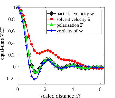
Figure 3: (Color online) Correlation functions for the solvent net flow $\tilde{{\bf u}}$, the polarization ${\bf P}$ the effective velocity $\tilde{{\bf w}}$ und the vorticity of $\tilde{{\bf w}}$ for small values of the coupling parameter $c_{\text{F}}=0.05$ (corresponds to large effective viscosities $\mu_{\mathrm{eff}}$). The remaining parameters are set to $c_{\text{I}}=2/3,\ \ell_{\text{p}}=10\;\mu m,\ \epsilon=1\;\mu m$. The length and the diameter of the bacteria are $\ell=5\;\mu m$ and $d=0.8\;\mu m$.

Next, we will show numerical results of the full model in spatially 3D for small values of the coupling parameter $c_{\text{F}}$ (large values of the effective viscosity $\mu_{\mathrm{eff}}$) to demonstrate that in this limit the overall collective dynamics of the bacterial suspension is dominated by its orientational dynamics.

For numerical simulations we use periodic boundary conditions and a pseudospectral code combined with an operator splitting technique for time integration where the linear operator is integrated exactly Dunkel et al. (2013a). To obtain the equal-time velocity correlation function, we consider a 2D slice in the middle of the 3D periodic cube and calculate the correlation functions in that plane averaged over 20 time-steps (for details see Dunkel et al. (2013a)).

Fig. 3 shows equal-time correlation functions for the scaled solvent flow $\tilde{{\bf u}}$, the polarization ${\bf P}$, the bacterial collective motion $\tilde{\bf w}$ and the vorticity of $\tilde{\bf w}$. The correlation functions for the collective bacterial motion and for the polarization collapse. This shows that, for large effective viscosities, the collective dynamics of the bacteria is dominated by the dynamics of the polarization. In this limit the collective dynamics is well described by the phenomenological model Eq. (1). It is also seen from the correlation functions that the typical vortex size (characterized by ranges with negative values) is induced by orientational order of the bacteria rather than the solvent dynamics.

To this end, the collective behavior of dense bacterial suspensions can be modeled by the one-fluid equation

$$\left(\partial_{t}+\lambda_{0}{\bf w}\cdot\nabla\right){\bf w}= - \nabla p-\alpha{\bf w}-\beta|{\bf w}|^{2}{\bf w}$$

$$+ \Gamma_{2}\nabla^{2}{\bf w}+\Gamma_{4}\nabla^{4}{\bf w},$$

$$\nabla\cdot{\bf w}= 0$$ , (77)

with parameters

$$\begin{split}\lambda_{0}&=\frac{3}{5}c_{\text{I}}\left(1+\frac{2}{3}a_{0}P_{\text{r}}c_{\text{F}}\right),\\ \alpha&=\left(1-c_{\text{I}}\right)/P_{\text{r}},\quad\beta=\frac{3}{5}c_{\text{I}}^{2}/P_{\text{r}},\\ \Gamma_{2}&=\frac{1}{10}\left(\frac{\epsilon}{\ell}\right)^{2}c_{\text{I}}/P_{\text{r}}-\frac{a_{0}}{15}P_{\text{r}}c_{\text{F}},\quad\Gamma_{4}=-\frac{a_{0}}{420}P_{\text{r}}c_{\text{F}}\end{split}$$ (78)

and abbreviations $c_{\text{I}}=8\pi\rho\gamma_{0}\epsilon^{3}\tau v_{0}/9$, $P_{\text{r}}=v_{0}\tau/\ell$, $c_{\text{F}}=f_{0}\rho\ell^{2}/(10\mu_{\mathrm{eff}}v_{0}).$ Again, time is scaled by $\ell/v_{0}$, space by $\ell$ and the collective velocity ${\bf w}$ by $v_{0}$.

Note that, for the derivation of the field equations, it was presumed that densities are large enough such that density fluctuations can be neglected. For dilute or semi-dilute microswimmer suspensions correlations or density fluctuations may play a significant role and can no longer be neglected Stenhammar et al. (2017). Near boundaries, such as walls or other obstacles, the assumption of constant swimmer density may also loose its justification due to effects like trapping Wensink and Löwen (2008); Hernandez-Ortiz et al. (2009). An extension of the theory to include such density variations will be presented elsewhere.

V Conclusions

The present article is devoted to the systematic derivation of generic field equations for the collective behavior of a large number of microswimmers in a Newtonian fluid.

Following earlier studies Hatwalne et al. (2004); Saintillan and Shelley (2009), the microswimmers are modeled by moving force dipoles that drive the ambient fluid and generate a net flow of the solvent. The new feature of the analysis presented here is the fact that we consider derivatives of the polar order parameter up to fourth order. Furthermore, we use a novel closure condition for the nematic order parameter that includes reorientations from active driving of the solvent flow by the microswimmers not present for passive particle systems. The derivation incorporates both, near field (polar and nematic) and far-field hydrodynamic interactions. The final equations comprise a dynamical equation for the polar order parameter ${\bf P}$ (averaged swimmer orientations) and the dynamics of the solvent flow ${\bf u}$. We restrict the derivation to sufficiently dense suspensions where density fluctuations play no significant role.

Parameters of the obtained field equations are directly linked to parameters of the microswimmer model. For example, the typical vortex size of swarming bacterial suspensions is given by $\Lambda=2\pi\sqrt{2\Gamma_{4}/\Gamma_{2}}$. In particular, in the limit of large self-swimming speeds, we find $\Lambda\propto\ell$, i.e., the vortex size depends linearly on the microswimmers’ length $\ell$. Indeed, such a dependency was recently found in experiments of B. subtilis suspensions Ilkanaiv et al. (2017).

The coupling between the solvent flow and the orientational dynamics depends strongly on the microscopic parameters, which motivates the introduction of a coupling parameter as a function of the parameters of the microswimmer model. We distinguish between two limiting cases:

For very weak coupling, the collective dynamics depends solely on the orientational dynamics. In this limit (and without boundary effects), the phenomenological model Eq. (1) describes the dynamics of the microswimmer suspension very well and the field equations derived in this paper can actually be reduced to the simpler model.

On the other hand, for a larger coupling parameter, the orientational dynamics couples to the solvent flow dynamics. Here, the intrinsic length scale set by $\Gamma_{2}$ and $\Gamma_{4}$ has less influence on the dynamical patterns.

It would be very interesting to observe such a dependence of the collective behaviour on the coupling (effective viscosity) in experiments.

Appendix A Mean field approximation of the interaction integral

According to Eq. (26) in the main text, the active part of the ”interaction integral” is given by

$$\mathcal{C}^{(2)}[\Phi^{\mathrm{act}}] = (S-1)\;{\nabla}_{\bf n}\cdot\left\{\int d{\bf n}^{\prime}\int d{{\bf x}^{\prime}}\;{\boldsymbol{\Pi}({\bf n})}\cdot\left[{\nabla}_{\bf n}\phi^{\mathrm{act}}({\bf n},{\bf n}^{\prime},|{\bf x}-{\bf x}^{\prime}|)\right]\;\mathcal{P}^{(2)}({\bf x},{\bf n};{\bf x}^{\prime},{\bf n}^{\prime},t)\right\}$$ (79)

$$= -\gamma_{0}v_{0}(S-1){\nabla}_{\bf n}\cdot\left\{{\boldsymbol{\Pi}({\bf n})}\cdot\int d{\bf n}^{\prime}\int_{|{\bf x}-{\bf x}^{\prime}|<\epsilon}d{{\bf x}^{\prime}}\;{\bf n}^{\prime}\;\mathcal{P}^{(2)}({\bf x},{\bf n};{\bf x}^{\prime},{\bf n}^{\prime},t)\right\}$$

where the second line has been obtained by inserting the expression for the activity-induced polar pair potential given in Eq. (3). We next approximate the two-particle distribution function $\mathcal{P}^{(2)}$, defined as

$$\mathcal{P}^{(2)}({\bf x},{\bf n};{\bf x}^{\prime},{\bf n}^{\prime},t)=\frac{1}{S^{2}}\sum_{\mu=1}^{S}\sum_{\nu=1}^{S}\bigg{\langle}\delta({\bf x}-{\bf X}^{\mu}(t))\,\delta({\bf n}-{\bf N}^{\mu}(t))\delta({\bf x}^{\prime}-{\bf X}^{\nu}(t))\,\delta({\bf n}^{\prime}-{\bf N}^{\nu}(t))\bigg{\rangle},$$ (80)

by factorization (mean-field approximation), i.e., $\mathcal{P}^{(2)}({\bf x},{\bf n};{\bf x}^{\prime},{\bf n}^{\prime},t)=\mathcal{P}({\bf x},{\bf n},t)\mathcal{P}({\bf x}^{\prime},{\bf n}^{\prime},t)$. In the limit $S\gg 1$ the integral then becomes

$$\mathcal{C}^{(2)}[\Phi^{\mathrm{act}}] \approx -\gamma_{0}v_{0}S{\nabla}_{\bf n}\cdot\left\{{\boldsymbol{\Pi}({\bf n})}\;\mathcal{P}({\bf x},{\bf n},t)\cdot\int d{\bf n}^{\prime}\int_{|{\bf x}-{\bf x}^{\prime}|<\epsilon}d{{\bf x}^{\prime}}\;{\bf n}^{\prime}\;\mathcal{P}({\bf x}^{\prime},{\bf n}^{\prime},t)\right\}$$ (81)

$$= -\gamma_{0}v_{0}{\nabla}_{\bf n}\cdot\left\{{\boldsymbol{\Pi}({\bf n})}\;\mathcal{P}({\bf x},{\bf n},t)\cdot\int_{|{\bf x}-{\bf x}^{\prime}|<\epsilon}d{{\bf x}^{\prime}}\;\rho({\bf x}^{\prime},t){\bf P}({\bf x}^{\prime},t)\right\},$$

where we have employed Eq. (17). To treat the spatial integral over the product $\rho{\bf P}$, we transform to the new integration variable $\boldsymbol{r}={\bf x}-{\bf x}^{\prime}$ and perform a Taylor expansion up to fourth order around $\boldsymbol{r}=0$. This yields

$$\boldsymbol{J}[\rho{\bf P}]=\int_{|{\bf x}-{\bf x}^{\prime}|<\epsilon}d{{\bf x}^{\prime}}\;\rho({\bf x}^{\prime},t){\bf P}({\bf x}^{\prime},t) = \int_{|\boldsymbol{r}|<\epsilon}d{\boldsymbol{r}}\;\rho({\bf x}-\boldsymbol{r},t){\bf P}({\bf x}-\boldsymbol{r},t)$$ (82)

$$\approx \int_{|\boldsymbol{r}|<\epsilon}d{\boldsymbol{r}}\;\left[1+\frac{1}{2!}\boldsymbol{r}\boldsymbol{r}:\nabla\nabla+\frac{1}{4!}\boldsymbol{r}\boldsymbol{r}\boldsymbol{r}\boldsymbol{r}::\nabla\nabla\nabla\nabla\right]\rho({\bf x},t){\bf P}({\bf x},t).$$

where we have truncated the expansion after the fourth-order term. The gradient operators acting on the product field $\rho{\bf P}$ can be taken out of the integral (since the result depends on ${\bf x}$ rather than on $\boldsymbol{r}$). Terms involving odd powers of $\boldsymbol{r}$ then vanish by symmetry, which has already been taken into account in writing the second line. The remaining integrals over even powers of $\boldsymbol{r}$ can be carried out analytically, yielding the non-zero coefficients in the fourth-order expansion of $\boldsymbol{J}[\rho{\bf P}]$, see Eqs. (III.1.2), (29) and (30) in the main text. Inserting the resulting expression into Eq. (81) one finally obtains Eq. (III.1.2).

The passive part of the interaction integral is treated in an analogous manner. We start from the definition [from Eq. (26)]

$$\mathcal{C}^{(2)}[\Phi^{\mathrm{pass}}] = (S-1)\;{\nabla}_{\bf n}\cdot\left\{\int d{\bf n}^{\prime}\int d{{\bf x}^{\prime}}\;{\boldsymbol{\Pi}({\bf n})}\cdot\left[{\nabla}_{\bf n}\phi^{\mathrm{pass}}({\bf n},{\bf n}^{\prime},|{\bf x}-{\bf x}^{\prime}|)\right]\;\mathcal{P}^{(2)}({\bf x},{\bf n};{\bf x}^{\prime},{\bf n}^{\prime},t)\right\}$$ (83)

$$= -\gamma_{1}(S-1){\nabla}_{\bf n}\cdot\left\{{\boldsymbol{\Pi}({\bf n})}\cdot\int d{\bf n}^{\prime}\int_{|{\bf x}-{\bf x}^{\prime}|<\epsilon}d{{\bf x}^{\prime}}\;{\bf n}^{\prime}({\bf n}^{\prime}\cdot{\bf n})\;\mathcal{P}^{(2)}({\bf x},{\bf n};{\bf x}^{\prime},{\bf n}^{\prime},t)\right\}$$

where we have used the passive (nematic) pair interaction given in Eq. (3). The mean-field approximation yields in the limit $S\gg 1$

$$\mathcal{C}^{(2)}[\Phi^{\mathrm{pass}}] \approx -\gamma_{1}S{\nabla}_{\bf n}\cdot\left\{{\boldsymbol{\Pi}({\bf n})}\;\mathcal{P}({\bf x},{\bf n},t)\cdot\int d{\bf n}^{\prime}\int_{|{\bf x}-{\bf x}^{\prime}|<\epsilon}d{{\bf x}^{\prime}}\;{\bf n}^{\prime}({\bf n}^{\prime}\cdot{\bf n})\;\mathcal{P}({\bf x}^{\prime},{\bf n}^{\prime},t)\right\}$$ (84)

$$= -\gamma_{1}{\nabla}_{\bf n}\cdot\left\{{\boldsymbol{\Pi}({\bf n})}\;\mathcal{P}({\bf x},{\bf n},t)\cdot\int_{|{\bf x}-{\bf x}^{\prime}|<\epsilon}d{{\bf x}^{\prime}}\;\rho({\bf x}^{\prime},t)\left({\bf Q}({\bf x}^{\prime},t)+\frac{1}{d}{\bf I}\right)\cdot{\bf n}\right\}$$

$$= -\gamma_{1}{\nabla}_{\bf n}\cdot\left\{{\boldsymbol{\Pi}({\bf n})}\;\mathcal{P}({\bf x},{\bf n},t)\cdot\int_{|{\bf x}-{\bf x}^{\prime}|<\epsilon}d{{\bf x}^{\prime}}\;\rho({\bf x}^{\prime},t){\bf Q}({\bf x}^{\prime},t)\cdot{\bf n}\right\},$$

where we have used that the contribution from the unit matrix in the second line vanishes due to the application of the projector ${\bf\Pi}$. The spatial integral is again treated by a Taylor expansion, that is,

$$\boldsymbol{J}[\rho{\bf Q}]=\int_{|{\bf x}-{\bf x}^{\prime}|<\epsilon}d{{\bf x}^{\prime}}\;\rho({\bf x}^{\prime},t){\bf Q}({\bf x}^{\prime},t)\approx\int_{|\boldsymbol{r}|<\epsilon}d{\boldsymbol{r}}\;\left[1+\frac{1}{2!}\boldsymbol{r}\boldsymbol{r}:\nabla\nabla+\frac{1}{4!}\boldsymbol{r}\boldsymbol{r}\boldsymbol{r}\boldsymbol{r}::\nabla\nabla\nabla\nabla\right]\rho({\bf x},t){\bf Q}({\bf x},t).$$ (85)

The remaining integrals are the same as those calculated for the active contribution. From this one obtains Eqs. (32) and (III.1.2) in the main text.

Appendix B Generalized closure conditions

In this work we use the Hand closure [Eq. (46)] to truncate the moment hierarchies in the equations for the polarization [see Eq. (38)], the nematic order parameter [see Eq. (41)] and the active stress [see Eq. (III.2.2)]. This is the simplest closure that is still consistent with the system’s symmetries. For the sake of completeness, we discuss a somewhat more sophisticated closure relation in the following, the so-called ”generalized quadratic closure” Kröger et al. (2008), of which the Hand closure and the quadratic closure are special cases. For nematic suspensions the quadratic closure should be used in order to obtain the Landau-de Gennes potential that ensures a relaxation into the nematic phase.

By introducing a parameter $s=0,1$ with $s=0$ referring to the Hand closure and $s=1$ referring to the quadratic closure, the relation for the moments of order $k\geq 3$ can be compactly written as

$$(\overline{n_{i}n_{j}n_{k}})^{\text{ST}} = s\left(P_{i}Q_{jk}\right)^{\text{ST}}$$ (86)

$$(\overline{n_{i}n_{j}n_{k}n_{l}})^{\text{ST}} = s\left(Q_{ij}Q_{kl}\right)^{\text{ST}}$$ (87)

$$(\overline{n_{i}n_{j}n_{k}n_{l}n_{m}})^{\text{ST}} = s\left(Q_{ij}\left[\overline{n_{k}n_{l}n_{m}}\right]\right)^{\text{ST}}.$$ (88)

Equations (86) - (88) are sufficient to express all higher moments in terms of the mean polarity ${\bf P}=\overline{{\bf n}}$ and the nematic order parameter ${\bf Q}=\overline{{\bf n}{\bf n}}-\mathbf{I}/d$. Note that all tensors on the left hand side are symmetric and traceless. To obtain from these tensors the corresponding full versions one may employ Eqs. (22) and (23). Specifically, for the Hand-Closure ($s=0$), we find for the third-order term

$$\overline{n_{i}n_{j}n_{k}}({\bf x},t) = \frac{3!}{2d+4}(\delta_{ij}\overline{n_{k}})^{\text{SY}}=\frac{1}{d+2}\left(\delta_{ij}\overline{n_{k}}+\delta_{ki}\overline{n_{j}}+\delta_{jk}\overline{n_{i}}\right)$$ (89)

and for the fourth-order term

$$\overline{n_{i}n_{j}n_{k}n_{l}}({\bf x},t) = \frac{4!}{4d+16}(\delta_{ij}\overline{n_{k}n_{l}})^{\text{SY}}-\frac{4!}{88d+16}(\delta_{ij}\delta_{kl})^{\text{SY}}$$ (90)

$$= \frac{1}{d+4}\left(\delta_{ij}\overline{n_{k}n_{l}}+\delta_{ik}\overline{n_{j}n_{l}}+\delta_{il}\overline{n_{k}n_{j}}+\delta_{kj}\overline{n_{i}n_{l}}+\delta_{lj}\overline{n_{k}n_{i}}+\delta_{kl}\overline{n_{i}n_{j}}\right)-$$

$$\frac{1}{11d+2}\left(\delta_{ij}\delta_{kl}+\delta_{ik}\delta_{jl}+\delta_{il}\delta_{kj}\right).$$

Finally, the fifth-order term (which is needed for the calculation of the active stress) becomes

$$\overline{n_{i}n_{j}n_{k}n_{l}n_{m}}({\bf x},t) = \frac{5!}{12d+72}(\delta_{ij}\overline{n_{k}n_{l}n_{m}})^{\text{SY}}-\frac{5!}{120d+144}(\delta_{ij}\delta_{kl}\overline{n_{m}})^{\text{SY}}$$ (91)

$$= \frac{5!}{(12d+72)(d+2)}(\delta_{ij}\left(\delta_{kl}\overline{n_{m}}+\delta_{mk}\overline{n_{l}}+\delta_{lm}\overline{n_{k}}\right))^{\text{SY}}-\frac{5!}{120d+144}(\delta_{ij}\delta_{kl}\overline{n_{m}})^{\text{SY}}$$

$$= \frac{5!}{(4d+24)(d+2)}(\delta_{ij}\delta_{kl}\overline{n_{m}})^{\text{SY}}-\frac{5!}{120d+144}(\delta_{ij}\delta_{kl}\overline{n_{m}})^{\text{SY}}$$

$$= \left[\frac{5!}{(4d+24)(d+2)}-\frac{5!}{120d+144}\right](\delta_{ij}\delta_{kl}\overline{n_{m}})^{\text{SY}}$$

$$= \left[\frac{1}{(4d+24)(d+2)}-\frac{1}{120d+144}\right]\times$$

$$4!\left(\left\{\delta_{ij}\delta_{kl}\right\}_{+}\overline{n_{m}}+\left\{\delta_{mj}\delta_{kl}\right\}_{+}\overline{n_{i}}+\left\{\delta_{im}\delta_{kl}\right\}_{+}\overline{n_{j}}+\left\{\delta_{ij}\delta_{ml}\right\}_{+}\overline{n_{k}}+\left\{\delta_{ij}\delta_{km}\right\}_{+}\overline{n_{l}}\right)$$

$$= \left[\frac{1}{6}\left(\frac{3}{2+d}-\frac{3}{6+d}-\frac{2}{6+5d}\right)\right]\times$$

$$\biggl{[}\left(\delta_{ij}\delta_{kl}+\delta_{ik}\delta_{jl}+\delta_{il}\delta_{kj}\right)\overline{n_{m}}+\left(\delta_{mj}\delta_{kl}+\delta_{mk}\delta_{jl}+\delta_{ml}\delta_{kj}\right)\overline{n_{i}}+$$

$$\left(\delta_{im}\delta_{kl}+\delta_{ik}\delta_{ml}+\delta_{il}\delta_{km}\right)\overline{n_{j}}+\left(\delta_{ij}\delta_{ml}+\delta_{im}\delta_{jl}+\delta_{il}\delta_{mj}\right)\overline{n_{k}}+$$

$$\left(\delta_{ij}\delta_{km}+\delta_{ik}\delta_{jm}+\delta_{im}\delta_{kj}\right)\overline{n_{l}}\biggr{]}.$$

Appendix C Detailed derivation of the field equations

C.1 Evolution equation for the polarization

We start from Eq. (38), which we display here again for clarity,

$$\begin{split}(\partial_{t}+{\bf u}\cdot\nabla){\bf P}=&{\bf\Omega}\cdot{\bf P}+a_{0}{\bf\Sigma}\cdot{\bf P}-v_{0}\nabla{\bf Q}+D\nabla^{2}{\bf P}-\frac{1}{\tau}{\bf P}-a_{0}{\bf\Sigma}:\overline{{\bf n}{\bf n}{\bf n}}\\ &+\gamma_{0}v_{0}\rho\frac{d-1}{d}\boldsymbol{J}[{\bf P}]-\gamma_{0}v_{0}\rho{\bf Q}\cdot\boldsymbol{J}[{\bf P}]+\gamma_{1}\rho\boldsymbol{J}[{\bf Q}]\cdot{\bf P}-\gamma_{1}\rho\boldsymbol{J}[{\bf Q}]:\overline{{\bf n}{\bf n}{\bf n}}.\end{split}$$ (92)

The terms involving third-order moments of ${\bf n}$ can be treated via the Hand closure (with $s=0$), where we utilize the explicit relations between full tensors and symmetric traceless parts given in Appendix B. In particular, we find with Eq. (89) in component form

$$\begin{split}\Sigma_{ij}\overline{n_{i}n_{j}n_{k}}=\Sigma_{ij}\frac{1}{d+2}(\delta_{ij}P_{k}+\delta_{ki}P_{j}+\delta_{jk}P_{i})=\frac{1}{d+2}(\Sigma_{kj}P_{j}+\Sigma_{ik}P_{i})=\frac{2}{d+2}\Sigma_{kj}P_{j}\,,\end{split}$$ (93)

$$\begin{split}J[{\bf Q}]_{ij}\overline{n_{i}n_{j}n_{k}}=J[{\bf Q}]_{ij}\frac{1}{d+2}(\delta_{ij}P_{k}+\delta_{ki}P_{j}+\delta_{jk}P_{i})=\frac{1}{d+2}(J[{\bf Q}]_{kj}P_{j}+J[{\bf Q}]_{ik}P_{i})=\frac{2}{d+2}J[{\bf Q}]_{kj}P_{j}\,.\end{split}$$ (94)

Inserting these results into Eq. (92) yields

$$\begin{split}(\partial_{t}+{\bf u}\cdot\nabla){\bf P}=&{\bf\Omega}\cdot{\bf P}+\frac{d}{d+2}a_{0}{\bf\Sigma}\cdot{\bf P}-v_{0}\nabla{\bf Q}+D\nabla^{2}{\bf P}-\frac{1}{\tau}{\bf P}\\ &+\gamma_{0}v_{0}\rho\frac{d-1}{d}\boldsymbol{J}[{\bf P}]-\gamma_{0}v_{0}\rho{\bf Q}\cdot\boldsymbol{J}[{\bf P}]+\frac{d}{d+2}\gamma_{1}\rho\boldsymbol{J}[{\bf Q}]\cdot{\bf P}.\end{split}$$ (95)

As a next step, we employ the closure relation for ${\bf Q}$ (see Eq. (47) in the main text), that is, ${\bf Q}=q\left({\bf P}{\bf P}\right)^{\text{ST}}+\lambda_{K}\boldsymbol{\Sigma}$. The divergence of ${\bf Q}$ then follows as

$$\nabla\cdot{\bf Q}=q\left({\bf P}\cdot\nabla{\bf P}-\frac{1}{d}\nabla|{\bf P}|^{2}\right)+\frac{\lambda_{K}}{2}\nabla^{2}{\bf u}.$$ (96)

Additionally, we insert the explicit forms of the quantities ${{\boldsymbol{J}}[{\bf P}]}$ and ${{\boldsymbol{J}}[{\bf Q}]}$ [see Eqs. (37] in the main text). Further, the products of the ${\bf Q}$-tensor and the quantities $\boldsymbol{J}$ become

$${\bf Q}\cdot\boldsymbol{J}[{\bf P}] = q\;{\bf P}{\bf P}\cdot\boldsymbol{J}[{\bf P}]-\frac{q}{d}|{\bf P}|^{2}\boldsymbol{J}[{\bf P}]+\lambda_{K}\boldsymbol{\Sigma}\cdot\boldsymbol{J}[{\bf P}]$$ (97)

$$= \frac{d-1}{d}qA_{d}|{\bf P}|^{2}{\bf P}+q\left({\bf P}\cdot\mathcal{D}{\bf P}\right){\bf P}-\frac{q}{d}|{\bf P}|^{2}\left(\mathcal{D}{\bf P}\right)+\lambda_{K}\boldsymbol{\Sigma}\cdot\boldsymbol{J}[{\bf P}],$$

and

$$\boldsymbol{J}[{\bf Q}]\cdot{\bf P}=A_{d}{\bf Q}\cdot{\bf P}+{\bf P}\cdot\mathcal{D}{\bf Q},$$ (98)

where we have introduced the operator $\mathcal{D}:=B_{d}\nabla^{2}+C_{d}\nabla^{4}$ including the constants defined in Eqs. (29) and (30) for $d=2,3$, respectively. Inserting Eqs. (37), (96), (97) and (98) into Eq. (95) we obtain

$$\left(\partial_{t}+{\bf u}\cdot\nabla\right){\bf P}= - v_{0}\frac{\lambda_{K}}{2}\nabla^{2}{\bf u}+\boldsymbol{\Omega}\cdot{\bf P}+\kappa\boldsymbol{\Sigma}\cdot{\bf P}-v_{0}q{\bf P}\cdot\nabla{\bf P}+\widetilde{\Gamma}_{2}\nabla^{2}{\bf P}+\widetilde{\Gamma}_{4}\nabla^{4}{\bf P}-\alpha{\bf P}-\beta|{\bf P}|^{2}{\bf P}+\frac{v_{0}}{d}q\nabla|{\bf P}|^{2}$$ (99)

$$- \gamma_{0}v_{0}q\rho\left({\bf P}\cdot\mathcal{D}{\bf P}\right)^{\text{ST}}{\bf P}-\gamma_{0}v_{0}\lambda_{K}\rho\boldsymbol{\Sigma}\cdot\mathcal{D}{\bf P}+\gamma_{1}\frac{d}{d+2}q\rho{\bf P}\cdot\left(\mathcal{D}{\bf P}{\bf P}\right)^{\text{ST}}+\gamma_{1}\frac{d}{d+2}\lambda_{K}\rho{\bf P}\cdot\mathcal{D}\boldsymbol{\Sigma},$$

where

$$\kappa = \frac{d}{d+2}a_{0}+\frac{d}{d+2}\gamma_{1}A_{d}\lambda_{K}\rho-\gamma_{0}v_{0}A_{d}\lambda_{K}\rho$$ (100)

$$\alpha = \frac{1}{\tau}-\frac{d-1}{d}\gamma_{0}v_{0}A_{d}\rho,$$ (101)

$$\beta = \left(\gamma_{0}v_{0}\frac{d-1}{d}-\gamma_{1}\frac{d-1}{d+2}\right)A_{d}q\rho$$ (102)

$$\widetilde{\Gamma}_{2} = D+\frac{d-1}{d}\gamma_{0}v_{0}B_{d},$$ (103)

$$\widetilde{\Gamma}_{4} = \frac{d-1}{d}\gamma_{0}v_{0}C_{d}.$$ (104)

Equation (99) can be somewhat simplified when we neglect the higher-order derivatives contained in the operator $\mathcal{D}$. This yields

$$\left(\partial_{t}+{\bf u}\cdot\nabla\right){\bf P}= - v_{0}\frac{\lambda_{K}}{2}\nabla^{2}{\bf u}+\boldsymbol{\Omega}\cdot{\bf P}+\kappa\boldsymbol{\Sigma}\cdot{\bf P}-v_{0}q{\bf P}\cdot\nabla{\bf P}+\widetilde{\Gamma}_{2}\nabla^{2}{\bf P}+\widetilde{\Gamma}_{4}\nabla^{4}{\bf P}+\alpha{\bf P}+\beta|{\bf P}|^{2}{\bf P}+\frac{v_{0}}{d}q\nabla|{\bf P}|^{2}.$$

Equation (C.1) still contains the flow field ${\bf u}$ and its derivatives.

C.2 Active stress and flow field expressed via the polarization

To proceed from Eq. (C.1), we now consider the average active stress given in Eq. (III.2.2). Using the Hand closure and the fact that, for constant density $\rho$, ${\bf P}=\overline{{\bf n}}$ is source-free [see Eq. (35)], that is, $\nabla\cdot\overline{{\bf n}}=0$, we find

$$\langle{\boldsymbol{\sigma}}^{a}({\bf x},t)\rangle \approx-f_{0}\rho\bigl{[} \zeta_{1}\overline{{\bf n}{\bf n}}+\zeta_{2}\;\nabla\cdot(\overline{{\bf n}{\bf n}{\bf n}})+\zeta_{3}\;{\nabla}{\nabla}:(\overline{{\bf n}{\bf n}{\bf n}{\bf n}})+\zeta_{4}\;\nabla\nabla\nabla:\cdot\,(\overline{{\bf n}{\bf n}{\bf n}{\bf n}{\bf n}})\bigr{]}$$ (106)

$$=-f_{0}\rho\bigl{\{} \xi_{1}\overline{{\bf n}{\bf n}}+\xi_{2}\left[\nabla\overline{{\bf n}}+(\nabla\overline{{\bf n}})^{\top}\right]+\xi_{3}\left[{\bf I}\nabla\nabla:\overline{{\bf n}{\bf n}}+2(\nabla\nabla\cdot\overline{{\bf n}{\bf n}})+2(\nabla\nabla\cdot\overline{{\bf n}{\bf n}})^{\top}+\nabla^{2}\overline{{\bf n}{\bf n}}\right]$$

$$+\xi_{4}\nabla^{2}\left[\nabla\overline{{\bf n}}+(\nabla\overline{{\bf n}})^{\top}\right]\bigr{\}},$$

where $\xi_{1}=\zeta_{1}=b_{r}+b_{f}$ and

$$\xi_{2}=\frac{\zeta_{2}}{d+2}\;,\qquad\xi_{3}=\frac{\zeta_{3}}{d+4}\;,\qquad\xi_{4}=\frac{\zeta_{4}\;}{2}\left(\frac{3}{2+d}-\frac{3}{6+d}-\frac{2}{6+5d}\right),$$ (107)

or explicitly in 2D (for $d=3$ see Eqs. (49) in Sec. III.2.3)

$$\xi_{2}=\frac{b_{r}^{2}-b_{f}^{2}}{8}\;,\qquad\xi_{3}=\frac{b_{r}^{3}+b_{f}^{3}}{36}\;,\qquad\xi_{4}=\frac{b_{r}^{4}-b_{f}^{4}}{192}.$$ (108)

Next, we re-express the second moment by the ${\bf Q}$-tensor and apply the closure relation for ${\bf Q}$ [see Eq. (47)]. We then obtain

$$\langle{\boldsymbol{\sigma}^{a}}({\bf x},t)\rangle \approx-f_{0}\rho\biggl{\{} \xi_{1}{\bf Q}+2\xi_{2}(\nabla{\bf P})^{\text{ST}}+2\xi_{4}\nabla^{2}(\nabla{\bf P})^{\text{ST}}+\;\xi_{3}\biggr{\{}\nabla^{2}{\bf Q}+4\left(\nabla\nabla\cdot{\bf Q}\right)^{\text{ST}}+\mathrm{Tr}\left[\nabla\nabla\cdot{\bf Q}\right]{\bf I}\biggr{\}}\biggl{\}}$$ (109)

$$=-f_{0}\rho\biggl{\{} \xi_{1}\left(q\left({\bf P}{\bf P}\right)^{\text{ST}}+\lambda_{K}\boldsymbol{\Sigma}+\frac{1}{d}{\bf I}\right)+2\xi_{2}\left(\nabla{\bf P}\right)^{\text{ST}}+2\xi_{4}\nabla^{2}\left(\nabla{\bf P}\right)^{\text{ST}}$$

$$+\xi_{3}\left(\frac{3}{2}\lambda_{K}\nabla^{2}\boldsymbol{\Sigma}+q\nabla^{2}\left({\bf P}{\bf P}\right)^{\text{ST}}+q\left(\nabla\nabla\cdot({\bf P}{\bf P})^{\text{ST}}\right)^{\text{ST}}\right)\biggl{\}}.$$

In what follows we neglect again nonlinear terms involving higher derivatives. We further assume that the strain rate varies only slowly in space, and thus, $\boldsymbol{\nabla}^{2}\Sigma\approx 0$. Equation (109) then becomes

$$\boldsymbol{\sigma}^{a}=-f_{0}\rho\biggl{\{}\xi_{1}\left(q\left({\bf P}{\bf P}\right)^{\text{ST}}+\lambda_{K}\boldsymbol{\Sigma}+\frac{1}{d}{\bf I}\right)+2\xi_{2}\left(\nabla{\bf P}\right)^{\text{ST}}+2\xi_{4}\nabla^{2}\left(\nabla{\bf P}\right)^{\text{ST}}\biggl{\}}.$$ (110)

This equation coincides with Eq. (48) in the main text. We now take the divergence of Eq. (110) and do the same for the passive stress, Eq. (43). Within the latter, we also use the closure relation for ${\bf Q}$. Inserting the resulting terms into the Stokes equation and solving for the velocity field we obtain (see Eq. (50) in the main text)

$$\nabla^{2}{\bf u}=\frac{1}{\mu_{\mathrm{eff}}}\left(f_{0}\rho\xi_{1}(1-\frac{\vartheta}{f_{0}\xi_{1}})q{\bf P}\cdot\nabla{\bf P}+f_{0}\rho\xi_{2}\nabla^{2}{\bf P}+f_{0}\rho\xi_{4}\nabla^{4}{\bf P}\right)+\nabla p_{\text{eff}}.$$ (111)

Inserting Eq. (111) into (C.1) we finally obtain the field equation for the polarization (see Eq. (53) in the main text).

Appendix D Evolution equation for the $\bf Q$-tensor and generalized Doi closure

To derive a self-consistent evolution equation for the $\bf Q$-tensor we start from Eq. (41), which we display here again for clarity,

$$\begin{split}\partial_{t}{\bf Q}=&-{\bf u}\cdot\nabla{\bf Q}-v_{0}(\nabla\cdot\overline{{\bf n}{\bf n}{\bf n}})^{\text{ST}}+D\nabla^{2}{\bf Q}-\frac{3}{\tau}{\bf Q}+2({\bf\Omega}\cdot{\bf Q})^{\text{ST}}+2a_{0}({\bf\Sigma}\cdot{\bf Q})^{\text{ST}}\\ &+\frac{2a_{0}}{d}{\bf\Sigma}-2a_{0}({\bf\Sigma}:\overline{{\bf n}{\bf n}{\bf n}{\bf n}})^{\text{ST}}+2\gamma_{0}v_{0}\rho(\boldsymbol{J}[{\bf P}]{\bf P})^{\text{ST}}-2\gamma_{0}v_{0}\rho(\boldsymbol{J}[{\bf P}]\cdot\overline{{\bf n}{\bf n}{\bf n}})^{\text{ST}}\\ &+2\gamma_{1}\rho(\boldsymbol{J}[{\bf Q}]\cdot{\bf Q})^{\text{ST}}+\frac{2\gamma_{1}\rho}{d}\boldsymbol{J}[{\bf Q}]-2\gamma_{1}\rho(\boldsymbol{J}[{\bf Q}]:\overline{{\bf n}{\bf n}{\bf n}{\bf n}})^{\text{ST}}\,.\end{split}$$ (112)

The terms involving third- and fourth-order moments of ${\bf n}$ can be treated via the Hand closure (with $s=0$), where we utilize the explicit relations between full tensors and symmetric traceless parts given in Appendix B. In particular, we find with Eq. (89) in component form

$$\left(\frac{\partial}{\partial x_{i}}\overline{n_{i}n_{j}n_{k}}\right)^{\text{ST}} = \frac{1}{d+2}\biggl{(}\frac{\partial}{\partial x_{i}}(\delta_{ij}P_{k}+\delta_{ki}P_{j}+\delta_{jk}P_{i})\biggr{)}^{\text{ST}}=\frac{2}{d+2}\left(\frac{\partial P_{k}}{\partial x_{j}}\right)^{\text{ST}},$$ (113)

and similarly

$$\left(J[{\bf P}]_{i}\overline{n_{i}n_{j}n_{k}}\right)^{\text{ST}} = \frac{1}{d+2}\biggl{(}J[{\bf P}]_{i}(\delta_{ij}P_{k}+\delta_{ki}P_{j}+\delta_{jk}P_{i})\biggr{)}^{\text{ST}}=\frac{2}{d+2}\left(J[{\bf P}]_{j}P_{k}\right)^{\text{ST}}.$$ (114)

With Eq. (90) we further find

$$\left(\Sigma_{ij}\overline{n_{i}n_{j}n_{k}n_{l}}\right)^{\text{ST}} = \left(\Sigma_{ij}\biggl{[}\frac{1}{d+4}\biggl{\{}\delta_{ij}Q_{kl}+\frac{1}{d}\delta_{ij}\delta_{kl}+\delta_{ik}Q_{jl}+\frac{1}{d}\delta_{ik}\delta_{jl}\right.$$ (115)

$$+\delta_{il}Q_{kj}+\frac{1}{d}\delta_{il}\delta_{kj}+\delta_{kj}Q_{il}+\frac{1}{d}\delta_{kj}\delta_{il}+\delta_{lj}Q_{kj}+\frac{1}{d}\delta_{lj}\delta_{ki}$$

$$\left.+\delta_{kl}Q_{ij}+\frac{1}{d}\delta_{kl}\delta_{ij}\biggl{\}}-\frac{1}{11d+2}(\delta_{ij}\delta_{kl}+\delta_{ik}\delta_{jl}+\delta_{il}\delta_{kj})\biggl{]}\right)^{\text{ST}}$$

$$= \frac{4}{d+4}\left(\Sigma_{kj}Q_{jl}\right)^{\text{ST}}-\left(\frac{2}{2+11d}-\frac{4}{d(d+4)}\right)\Sigma_{kl},$$

and similarly

$$\left(J[{\bf Q}]_{ij}\overline{n_{i}n_{j}n_{k}n_{l}}\right)^{\text{ST}} = \frac{4}{d+4}\left(J[{\bf Q}]_{kj}Q_{jl}\right)^{\text{ST}}-\left(\frac{2}{2+11d}-\frac{4}{d(d+4)}\right)J[{\bf Q}]_{kl}.$$ (116)

Inserting these relations into Eq. (112) yields

$$\partial_{t}{\bf Q}= - {\bf u}\nabla\cdot{\bf Q}+2\boldsymbol{\Omega}\cdot{\bf Q}+D\nabla^{2}{\bf Q}-\frac{2}{d+2}v_{0}\left(\nabla{\bf P}\right)^{\text{ST}}-\frac{3}{\tau}{\bf Q}+\frac{2a_{0}}{d+2}\boldsymbol{\Sigma}+\frac{d}{d+4}2a_{0}\left(\boldsymbol{\Sigma}\cdot{\bf Q}\right)^{\text{ST}}$$ (117)

$$+ \frac{d}{d+2}2\gamma_{0}v_{0}\rho\left(\boldsymbol{J}[{\bf P}]{\bf P}\right)^{\text{ST}}+\frac{2\gamma_{1}\rho}{d+2}{\boldsymbol{J}[{\bf Q}]}+\frac{d}{d+4}2\gamma_{1}\rho\left(\boldsymbol{J}[{\bf Q}]\cdot{\bf Q}\right)^{\text{ST}},$$

where we have used the relation

$$\frac{1}{d}+\frac{2}{2+11d}-\frac{4}{d(d+4)}=\frac{1}{d+2},$$ (118)

which is valid for $d=2,3$, i.e., only for systems in two- or three-dimensional space.

Eq. (117) already provides a self-consistent relation for the time evolution of the $\bf Q$-tensor for given polarization and flow field. For active nematics, higher moments have to be approximated by the quadratic closure (see Appendix B).

We now proceed towards a derivation of the generalized Doi closure in Eq. (47). To this end we insert the explicit expressions for the quantities ${{\boldsymbol{J}}[{\bf P}]}$ and ${{\boldsymbol{J}}[{\bf Q}]}$ [see Eqs. (37)] into Eq. (117). Henceforth, we only keep terms of linear order in $\bf Q$ and $\bf\Sigma$ and quadratic order in $\bf P$. Further, we neglect all gradient terms. We now assume that the dynamics of $\bf Q$ is much faster than the dynamics of the polar order parameter $\bf{P}$, such that $\partial_{t}{\bf Q}=0$. With these assumptions, we obtain from Eq. (117)

$${\bf Q}=q\left({\bf P}{\bf P}\right)^{\text{ST}}+\lambda_{K}\boldsymbol{\Sigma},$$ (119)

which has exactly the form of the generalized Doi closure (47). Within this derivation the coefficients $q$ and $\lambda_{K}$ are calculated via

$$q=\left(2v_{0}\gamma_{0}A_{d}\rho\frac{d}{d+2}\right)\bigg{/}\left(\frac{3}{\tau}-\frac{2\gamma_{1}\rho A_{d}}{d+2}\right)$$ (120)

and

$$\lambda_{K}=\left(\frac{2a_{0}}{d+2}\right)\bigg{/}\left(\frac{3}{\tau}-\frac{2\gamma_{1}\rho A_{d}}{d+2}\right),$$ (121)

or explicitly in 3D

$$q=\frac{v_{0}\gamma_{0}A_{3}\rho\tau}{5/2-\gamma_{1}\rho A_{3}\tau/3}\qquad\text{and}\qquad\lambda_{K}=\frac{a_{0}\tau}{15/2-\gamma_{1}\rho A_{3}\tau}.$$ (122)

References

• Sumino et al. (2012) Y. Sumino, K. H. Nagai, Y. Shitaka, D. Tanaka, K. Yoshikawa, H. Chaté,  and K. Oiwa, Nature 483, 448 (2012).
• Schaller et al. (2010) V. Schaller, C. Weber, C. Semmrich, E. Frey,  and A. R. Bausch, Nature 467, 73 (2010).
• Nishiguchi and Sano (2015) D. Nishiguchi and M. Sano, Phys. Rev. E 92, 052309 (2015).
• Rabani et al. (2013) A. Rabani, G. Ariel,  and A. Be’er, PLOS ONE 8, 1 (2013).
• Buttinoni et al. (2013) I. Buttinoni, J. Bialké, F. Kümmel, H. Löwen, C. Bechinger,  and T. Speck, Phys. Rev. Lett. 110, 238301 (2013).
• Peruani et al. (2012) F. Peruani, J. Starruß, V. Jakovljevic, L. Søgaard-Andersen, A. Deutsch,  and M. Bär, Phys. Rev. Lett. 108, 098102 (2012).
• Simha and Ramaswamy (2002) R. A. Simha and S. Ramaswamy, Phys. Rev. Lett. 89, 058101 (2002).
• Zhang et al. (2010) H.-P. Zhang, A. Be’er, E.-L. Florin,  and H. L. Swinney, Proc. Natl. Acad. Sci. U.S.A. 107, 13626 (2010).
• Schwarz-Linek et al. (2012) J. Schwarz-Linek, C. Valeriani, A. Cacciuto, M. Cates, D. Marenduzzo, A. Morozov,  and W. Poon, Proc. Natl. Acad. Sci. U.S.A. 109, 4052 (2012).
• Wittkowski et al. (2014) R. Wittkowski, A. Tiribocchi, J. Stenhammar, R. J. Allen, D. Marenduzzo,  and M. E. Cates, Nat. Commun. 5, 4351 (2014).
• Speck et al. (2014) T. Speck, J. Bialké, A. M. Menzel,  and H. Löwen, Phys. Rev. Lett. 112, 218304 (2014).
• Dombrowski et al. (2004) C. Dombrowski, L. Cisneros, S. Chatkaew, R. E. Goldstein,  and J. O. Kessler, Phys. Rev. Lett. 93, 098103 (2004).
• Bratanov et al. (2015) V. Bratanov, F. Jenko,  and E. Frey, Proc. Natl. Acad. Sci. U.S.A. 112, 15048 (2015).
• Oza et al. (2016) A. U. Oza, S. Heidenreich,  and J. Dunkel, Eur. Phys. J. E 39, 97 (2016).
• Heidenreich et al. (2014) S. Heidenreich, S. H. Klapp,  and M. Bär, J. Phys. Conf. Ser. 490, 012126 (2014).
• Ramaswamy (2010) S. Ramaswamy, Annu. Rev. Condens. Matter Phys. 1, 323 (2010).
• Romanczuk et al. (2012) P. Romanczuk, M. Bär, W. Ebeling, B. Lindner,  and L. Schimansky-Geier, Eur. Phys. J. Spec. Top. 202, 1 (2012).
• Marchetti et al. (2013) M. Marchetti, J. Joanny, S. Ramaswamy, T. Liverpool, J. Prost, M. Rao,  and R. A. Simha, Rev. Mod. Phys. 85, 1143 (2013).
• Elgeti et al. (2015) J. Elgeti, R. G. Winkler,  and G. Gompper, Rep. Prog. Phys. 78, 056601 (2015).
• Bechinger et al. (2016) C. Bechinger, R. Di Leonardo, H. Löwen, C. Reichhardt, G. Volpe,  and G. Volpe, Rev. Mod. Phys. 88, 045006 (2016).
• Zöttl and Stark (2016) A. Zöttl and H. Stark, J. Phys. Condens. Matter 28, 253001 (2016).
• Menzel (2015) A. M. Menzel, Phys. Rep. 554, 1 (2015).
• Peshkov et al. (2012a) A. Peshkov, I. S. Aranson, E. Bertin, H. Chaté,  and F. Ginelli, Phys. Rev. Lett. 109, 268701 (2012a).
• Peshkov et al. (2012b) A. Peshkov, S. Ngo, E. Bertin, H. Chaté,  and F. Ginelli, Phys. Rev. Lett. 109, 098101 (2012b).
• Baskaran and Marchetti (2008) A. Baskaran and M. C. Marchetti, Phys. Rev. E 77, 011920 (2008).
• Ahmadi et al. (2005) A. Ahmadi, T. B. Liverpool,  and M. C. Marchetti, Phys. Rev. E 72, 060901 (2005).
• Grossmann et al. (2012) R. Grossmann, L. Schimansky-Geier,  and P. Romanczuk, New J. Phys. 14, 073033 (2012).
• Menzel et al. (2016) A. M. Menzel, A. Saha, C. Hoell,  and H. Löwen, J. Chem. Phys. 144, 024115 (2016).
• Saintillan and Shelley (2008) D. Saintillan and M. J. Shelley, Phys. Rev. Lett. 100, 178103 (2008).
• Saintillan and Shelley (2009) D. Saintillan and M. J. Shelley, C. R. Physique 14, 497 (2009).
• Toner and Tu (1998) J. Toner and Y. Tu, Phys. Rev. E 58, 4828 (1998).
• Großmann et al. (2014) R. Großmann, P. Romanczuk, M. Bär,  and L. Schimansky-Geier, Phys. Rev. Lett. 113, 258104 (2014).
• Großmann et al. (2015) R. Großmann, P. Romanczuk, M. Bär,  and L. Schimansky-Geier, Eur. Phys. J. Spec. Top. 224, 1325 (2015).
• Sanchez et al. (2012) T. Sanchez, D. T. Chen, S. J. DeCamp, M. Heymann,  and Z. Dogic, Nature 491, 431 (2012).
• Zhou et al. (2014) S. Zhou, A. Sokolov, O. D. Lavrentovich,  and I. S. Aranson, Proc. Natl. Acad. Sci. U.S.A. 111, 1265 (2014).
• Genkin et al. (2017) M. M. Genkin, A. Sokolov, O. D. Lavrentovich,  and I. S. Aranson, Phys. Rev. X 7, 011029 (2017).
• Hemingway et al. (2016) E. J. Hemingway, P. Mishra, M. C. Marchetti,  and S. M. Fielding, Soft Matter 12, 7943 (2016).
• Doostmohammadi et al. (2016) A. Doostmohammadi, M. F. Adamer, S. P. Thampi,  and J. M. Yeomans, Nat. Commun. 7, 10557 (2016).
• Wensink et al. (2012) H. H. Wensink, J. Dunkel, S. Heidenreich, K. Drescher, R. E. Goldstein, H. Löwen,  and J. M. Yeomans, Proc. Natl. Acad. Sci. U.S.A. 109, 14308 (2012).
• Vicsek et al. (1995) T. Vicsek, A. Czirók, E. Ben-Jacob, I. Cohen,  and O. Shochet, Phys. Rev. Lett. 75, 1226 (1995).
• Dunkel et al. (2013a) J. Dunkel, S. Heidenreich, K. Drescher, H. H. Wensink, M. Bär,  and R. E. Goldstein, Phys. Rev. Lett. 110, 228102 (2013a).
• Dunkel et al. (2013b) J. Dunkel, S. Heidenreich, M. Bär,  and R. E. Goldstein, New J. Phys. 15, 045016 (2013b).
• Zhang et al. (2009) H. Zhang, A. Be’Er, R. S. Smith, E.-L. Florin,  and H. L. Swinney, EPL 87, 48011 (2009).
• Lushi et al. (2014) E. Lushi, H. Wioland,  and R. E. Goldstein, Proc. Natl. Acad. Sci. U.S.A. 111, 9733 (2014).
• Heidenreich et al. (2016) S. Heidenreich, J. Dunkel, S. H. L. Klapp,  and M. Bär, Phys. Rev. E 94, 020601 (2016).
• Drescher et al. (2011) K. Drescher, J. Dunkel, L. H. Cisneros, S. Ganguly,  and R. E. Goldstein, Proc. Natl. Acad. Sci. U.S.A. 108, 10940 (2011).
• Happel and Brenner (2012) J. Happel and H. Brenner, Low Reynolds number hydrodynamics: with special applications to particulate media, Vol. 1 (Springer Science & Business Media, 2012).
• Ginelli et al. (2010) F. Ginelli, F. Peruani, M. Bär,  and H. Chaté, Phys. Rev. Lett. 104, 184502 (2010).
• Yang et al. (2010) Y. Yang, V. Marceau,  and G. Gompper, Phys. Rev. E 82, 031904 (2010).
• Wensink and Löwen (2008) H. H. Wensink and H. Löwen, Phys. Rev. E 78, 031409 (2008).
• Peruani et al. (2006) F. Peruani, A. Deutsch,  and M. Bär, Phys. Rev. E 74, 030904 (2006).
• Großmann et al. (2016) R. Großmann, F. Peruani,  and M. Bär, Phys. Rev. E 93, 040102 (2016).
• Najafi and Golestanian (2004) A. Najafi and R. Golestanian, Phys. Rev. E 69, 062901 (2004).
• Pooley et al. (2007) C. M. Pooley, G. P. Alexander,  and J. M. Yeomans, Phys. Rev. Lett. 99, 228103 (2007).
• Avron et al. (2005) J. Avron, O. Kenneth,  and D. Oaknin, New J. Phys. 7, 234 (2005).
• Maier and Saupe (1958) W. Maier and A. Saupe, Z. Naturforsch. A 13, 564 (1958).
• Maier and Saupe (1959) W. Maier and A. Saupe, Z. Naturforsch. A 14, 882 (1959).
• Maier and Saupe (1960) W. Maier and A. Saupe, Z. Naturforsch. A 15, 287 (1960).
• Jeffery (1922) G. B. Jeffery, Proc. R. Soc. Lond. A 102, 161 (1922).
• Hinch and Leal (1979) E. J. Hinch and L. G. Leal, J. Fluid Mech. 92, 591 (1979).
• Pedley and Kessler (1992) T. Pedley and J. O. Kessler, Annu. Rev. Fluid Mech. 24, 313 (1992).
• Rafaï et al. (2010) S. Rafaï, L. Jibuti,  and P. Peyla, Phys. Rev. Lett. 104, 098102 (2010).
• Jibuti et al. (2017) L. Jibuti, W. Zimmermann, S. Rafaï,  and P. Peyla, Phys. Rev. E 96, 052610 (2017).
• Hinch (2010) J. Hinch, J. Fluid Mech. 663, 8 (2010).
• Einstein (1906) A. Einstein, Ann. Phys. 324, 289 (1906).
• Batchelor (1974) G. Batchelor, Annu. Rev. Fluid Mech. 6, 227 (1974).
• Haines et al. (2008) B. M. Haines, I. S. Aranson, L. Berlyand,  and D. A. Karpeev, Phys. Biol. 5, 046003 (2008).
• Krieger and Dougherty (1959) I. M. Krieger and T. J. Dougherty, Trans. Soc. Rheol. 3, 137 (1959).
• Brinkmann (1949) H. C. Brinkmann, Appl. Sci. Res. 1, 27 (1949).
• Hatwalne et al. (2004) Y. Hatwalne, S. Ramaswamy, M. Rao,  and R. A. Simha, Phys. Rev. Lett. 92, 118101 (2004).
• Baskaran and Marchetti (2009) A. Baskaran and M. C. Marchetti, Proc. Natl. Acad. Sci. U.S.A. 106, 15567 (2009).
• Spagnolie and Lauga (2012) S. E. Spagnolie and E. Lauga, J. Fluid Mech. 700, 105 (2012).
• Dhont and Briels (2002) J. K. G. Dhont and W. J. Briels, J. Chem. Phys. 117, 3992 (2002).
• McCourt et al. (1990) F. R. W. McCourt, J. J. M. Beenakker, W. Köhler,  and I. Kus̆c̆er, Nonequilibrium Phenomena in Polyatomic Gases (Clarendon Press, Oxford 1990).
• Turzi (2011) S. Turzi, J. Math. Phys. 52, 053517 (2011).
• Kröger et al. (2008) M. Kröger, A. Ammar,  and F. Chinesta, J. Non-Newtonian Fluid Mech. 149, 40 (2008).
• Hess (2015) S. Hess, Tensors for physics (Springer, 2015).
• Risken (1984) H. Risken, The Fokker-Planck Equation (Springer, 1984).
• Jacobs (2010) K. Jacobs, Stochastic processes for physicists: understanding noisy systems (Cambridge University Press, 2010).
• Ilg et al. (1999) P. Ilg, I. V. Karlin,  and H. C. Öttinger, Phys. Rev. E 60, 5783 (1999).
• Masao (1981) D. Masao, J. Polym. Sci. Part B Polym. Phys. 19, 229 (1981).
• Hess (1976) S. Hess, Z. Naturforsch. A 31, 1034 (1976).
• Hand (1962) G. L. Hand, J. Fluid Mech. 13, 33 (1962).
• Rinäcker and Hess (1998) G. Rinäcker and S. Hess, Physica A 267, 294 (1998).
• Doi and Edwards (1988) M. Doi and S. F. Edwards, The theory of polymer dynamics, Vol. 73 (Oxford University Press, 1988).
• Heidenreich (2009) S. Heidenreich, Orientational dynamics and flow properties of polar and non-polar hard-rod fluids, Ph.D. thesis, Technische Universität Berlin (2009).
• Hess (1975) S. Hess, Z. Naturforsch. A 30, 1224 (1975).
• Pujolle-Robic and Noirez (2001) C. Pujolle-Robic and L. Noirez, Nature 409, 167 (2001).
• Olmsted and Goldbart (1990) P. D. Olmsted and P. Goldbart, Phys. Rev. A 41, 4578(R) (1990).
• Cappelaere et al. (1997) E. Cappelaere, J. F. Berret, J. P. Decruppe, R. Cressely,  and P. Lindner, Phys. Rev. E 56, 1869 (1997).
• Fischer and Callaghan (2001) E. Fischer and P. T. Callaghan, Phys. Rev. E 64, 011501 (2001).
• Wolgemuth (2008) C. W. Wolgemuth, Biophys. J. 95, 1564 (2008).
• Sokolov and Aranson (2009) A. Sokolov and I. S. Aranson, Phys. Rev. Lett. 103, 148101 (2009).
• Stenhammar et al. (2017) J. Stenhammar, C. Nardini, R. W. Nash, D. Marenduzzo,  and A. Morozov, Phys. Rev. Lett. 119, 028005 (2017).
• Hernandez-Ortiz et al. (2009) J. P. Hernandez-Ortiz, P. T. Underhill,  and M. D. Graham, J. Phys. Condens. Matter 21, 204107 (2009).
• Ilkanaiv et al. (2017) B. Ilkanaiv, D. B. Kearns, G. Ariel,  and A. Be’er, Phys. Rev. Lett. 118, 158002 (2017).