Boundaries of Amplituhedra and NMHV Symbol Alphabets at Two Loops

Abstract

In this sequel to arXiv:1711.11507 we classify the boundaries of amplituhedra relevant for determining the branch points of general two-loop amplitudes in planar $\mathcal{N}=4$ super-Yang–Mills theory. We explain the connection to on-shell diagrams, which serves as a useful cross-check. We determine the branch points of all two-loop NMHV amplitudes by solving the Landau equations for the relevant configurations and are led thereby to a conjecture for the symbol alphabets of all such amplitudes.

1 Introduction

It has been a long-standing goal to determine scattering amplitudes in quantum field theory from knowledge of their analytic structure coupled with other basic physical and mathematical input. In planar $\mathcal{N}=4$ super-Yang–Mills theory (which we refer to as SYM theory), the current state of the art for carrying out explicit computations of multi-loop amplitudes is a bootstrap program that relies fundamentally on assumptions about the location of branch points of certain amplitudes.

The aim of the research program initiated in Dennen:2015bet ; Dennen:2016mdk for MHV amplitudes and generalized to non-MHV amplitudes in Prlina:2017azl (to which this paper should be considered a sequel) is to provide an a priori derivation of the set of branch points for any given amplitude. For sufficiently simple amplitudes in SYM theory this information can go a long way by leading to natural guesses for the symbol alphabets Goncharov:2010jf of various amplitudes. The possibility to do so exists because of the simple fact pointed out in Maldacena:2015iua that the locus in the space of external data $\operatorname{Conf}_{n}(\mathbb{P}^{3})$ where the symbol letters of a given amplitude vanish should be the same as the locus where the corresponding Landau equations Landau:1959fi ; ELOP admit solutions. A slight refinement of this statement, to account for the fact that amplitudes in general have algebraic branch cuts in addition to logarithmic cuts, was discussed in Sec. 7 of Prlina:2017azl .

The hexagon bootstrap program, which has succeeded in computing all six-point amplitudes through five loops Dixon:2011pw ; Dixon:2011nj ; Dixon:2013eka ; Dixon:2015iva ; Caron-Huot:2016owq , relies on the hypothesis that these amplitudes can have branch points only at nine specific loci in the space of external data $\operatorname{Conf}_{6}(\mathbb{P}^{3})$. Similarly the heptagon bootstrap Drummond:2014ffa , which has revealed the symbols of the seven-point four-loop MHV and three-loop NMHV amplitudes Dixon:2016nkn , assumes 42 particular branch points. Ultimately we may hope for an all-loop proof of these hypotheses about six- and seven-point amplitudes, but in this paper we focus on the less ambitious goal of deriving the singularity loci for all two-loop NMHV amplitudes in SYM theory. The result, summarized in Sec. 5.3, leads to a natural conjecture for the symbol alphabets of these amplitudes which we hope may be employed in the near future by bootstrappers eager to study this class of amplitudes.

The rest of this paper is organized as follows. In Sec. 2 we develop a procedure for constructing certain boundaries of two-loop amplituhedra by “merging” one-loop configurations of the type classified in the prequel Prlina:2017azl . In Sec. 3 we organize the results according to helicity and codimensionality (the number of on-shell conditions satisfied by each configuration) and discuss some subtleties about overconstrained configurations that require resolution. Section 4 discusses the connection between branches of solutions to on-shell conditions and on-shell diagrams, which provides a useful cross-check of our classification. In Sec. 5 we discuss the analysis of the Landau equations for configurations relevant for NMHV amplitudes and, in Eqns. (51) and (52), we present a conjecture for the symbol alphabets of all two-loop NMHV amplitudes.

2 Classification of Two-Loop Boundaries

In this section we classify certain boundaries of two-loop amplituhedra. This analysis builds heavily on Sections 3–5 of Prlina:2017azl , and in particular we show how to recycle the one-loop boundaries classified there by “merging” pairs of one-loop boundaries into two-loop boundaries. We find that two different formulations of the amplituhedron — the original formulation in terms of $C$ and $D$ matrices Arkani-Hamed:2013jha , and the reformulation in terms of sign flips Arkani-Hamed:2017vfh — play two complementary roles, exactly as in Prlina:2017azl . Specifically, the former is useful for establishing the existence of boundaries by constructing explicit $C$ and $D$ matrix representatives, while the latter is useful for establishing the non-existence of any other boundaries.

Before proceeding let us dispense of some important details that would otherwise overcomplicate our exposition. There is a parity symmetry between $A_{n,\textrm{k},L}$, the $n$-point, $\textrm{N}^{k}\textrm{MHV}$, $L$-loop amplitude in SYM theory, and its parity conjugate $A_{n,n-\textrm{k}-4,L}$. For fixed $n$, amplitudes become increasingly complicated as k is increased from zero, but after $\textrm{k}\sim n/2$ they must begin to decrease in complexity until the upper bound $\textrm{k}=n-4$. In what follows we will often make use of lower bounds on k, or on constructions that increment k by 1. In making these arguments, we always have in mind that k is sufficiently small compared to $n$. In other words, unless otherwise stated, we are always working in the “low-k” regime, to use the terminology of Prlina:2017azl . At the very end of our analysis, once we have all of the desired results in this regime, we appeal to parity symmetry in order to translate low-k results into high-k results. However the details of matching these two regimes near the midpoint $\textrm{k}\sim n/2$ can be quite intricate, even moreso at two loops than it was in the one-loop analysis of Prlina:2017azl .

2.1 Identifying the Relevant Boundaries

In general, a configuration $(Y,\mathcal{L}^{(1)},\mathcal{L}^{(2)})$ lies on a boundary of a two-loop amplituhedron if at least one item on the following menu is satisfied:

1. $Y$ is such that some four-brackets of the form $\langle a\,a{+}1\,b\,b{+}1\rangle$ vanish,

2. $\mathcal{L}^{(1)}$ satisfies some on-shell conditions $\langle\mathcal{L}^{(1)}\,a_{1}\,a_{1}{+}1\rangle=\cdots=\langle\mathcal{L}^{(1)}\,a_{d_{1}}\,a_{d_{1}}{+}1\rangle=0$,

3. $\mathcal{L}^{(2)}$ satisfies some on-shell conditions $\langle\mathcal{L}^{(2)}\,b_{1}\,b_{1}{+}1\rangle=\cdots=\langle\mathcal{L}^{(2)}\,b_{d_{2}}\,b_{d_{2}}{+}1\rangle=0$,

4. or $\langle\mathcal{L}^{(1)}\,\mathcal{L}^{(2)}\rangle=0$.

Above and through the remainder of the paper, we always take $\langle ABCD\rangle\equiv[YABCD]$ — what we call projected four-brackets following Arkani-Hamed:2017vfh .

For the purpose of finding Landau singularities we are always interested only in loop momenta $(\mathcal{L}^{(1)},\mathcal{L}^{(2)})$ that exist for generic projected external data, i.e., for generic $Y$, so we disregard possibility (1) in all that follows. Next, we note that for configurations which do not satisfy (4), the Landau equations decouple into two separate sets of equations on the two individual loop momenta, so there can be no new Landau singularities beyond those already found at one loop. Therefore in all that follows we only consider boundaries on which $\langle\mathcal{L}^{(1)}\,\mathcal{L}^{(2)}\rangle=0$. The Landau equations similarly degenerate if either $d_{1}$ or $d_{2}$ (defined in the preceeding paragraph) is zero, so we are only interested in configurations with $d_{1}d_{2}>0$.

The above considerations motivate us to define an $\mathcal{L}$-boundary of a two-loop amplituhedron as a configuration $(Y,\mathcal{L}^{(1)},\mathcal{L}^{(2)})$ for which $Y$ is such that the projected external data are generic, $\langle\mathcal{L}^{(1)}\,\mathcal{L}^{(2)}\rangle=0$, and each $\mathcal{L}$ satisfies at least one on-shell condition of the form $\langle\mathcal{L}\,a\,a{+}1\rangle=0$. In particular, these conditions imply that both $(Y,\mathcal{L}^{(1)})$ and $(Y,\mathcal{L}^{(2)})$ must lie on boundaries of some one-loop amplituhedra; each of these must therefore be one of the 19 branches tabulated in Tab. 1 of Prlina:2017azl .

2.2 Merging One-Loop Boundaries

The preceding analysis suggests that the boundaries of two-loop amplituhedra can be understood by merging various one-loop boundaries. Let us now see how this works in detail. Suppose that $(Y^{(1)},\mathcal{L}^{(1)})$ and $(Y^{(2)},\mathcal{L}^{(2)})$ lie on boundaries of $\mathcal{A}_{n,\textrm{k}_{1},1}$ and $\mathcal{A}_{n,\textrm{k}_{2},1}$, respectively. Then they can be represented as $Y^{(\alpha)}=C^{(\alpha)}\mathcal{Z}$ and $\mathcal{L}^{(\alpha)}=D^{(\alpha)}\mathcal{Z}$, where for each $\alpha\in\{1,2\}$, the matrices $C^{(\alpha)}$, $\left(\begin{smallmatrix}D^{(\alpha)}\\ C^{(\alpha)}\end{smallmatrix}\right)$, and $D^{(\alpha)}$ (as shown in Prlina:2017azl ), are all non-negative. In order to streamline the argument we initially consider $\textrm{k}_{1}$ and $\textrm{k}_{2}$ to be the smallest values of helicity for which boundaries of the desired class exist, and we take each pair $(C^{(\alpha)},D^{(\alpha)})$ to have the form of one of the 19 branches shown in Secs. 4.2 through 4.4 of Prlina:2017azl . We will show that such a pair of valid one-loop boundary configurations can be uplifted into a valid two-loop boundary configuration $(C,D^{(1)},D^{(2)})$ satisfying $\langle\mathcal{L}^{(1)}\,\mathcal{L}^{(2)}\rangle=0$ by constructing an appropriate matrix $C$ from $C^{(1)}$ and $C^{(2)}$.

The process of merging two boundaries depends on whether the two loop momenta $\mathcal{L}^{(1)}$, $\mathcal{L}^{(2)}$ each pass through some common external point $Z_{i}$. If they do, then we say that they manifestly intersect and the condition that $\langle\mathcal{L}^{(1)}\,\mathcal{L}^{(2)}\rangle=0$ is automatically satisfied. In this case we can simply stack the two individual $C$-matrices on top of each other in order to form

$$C=\left(\begin{matrix}C^{(1)}\\ C^{(2)}\end{matrix}\right).$$ (1)

If, on the other hand, the two loop momenta do not manifestly intersect, then we can still ensure that $\langle\mathcal{L}^{(1)}\,\mathcal{L}^{(2)}\rangle=[(C\mathcal{Z})\,\mathcal{L}^{(1)}\,\mathcal{L}^{(2)}]=0$ by adding one additional suitably crafted row to $C$. Specifically, if $A^{(\alpha)}$, $B^{(\alpha)}$ are any four points in $\mathbb{P}^{n}$ such that $\mathcal{L}^{(\alpha)}=(A^{(\alpha)}\mathcal{Z},B^{(\alpha)}\mathcal{Z})$, then adding a row to $C$ that is any linear combination of these four points will guarantee that $\langle\mathcal{L}^{(1)}\,\mathcal{L}^{(2)}\rangle=0$.

In this manner we have constructed a candidate for a configuration on the boundary of $\mathcal{A}_{n,\textrm{k},2}$ with $\textrm{k}=\textrm{k}_{1}+\textrm{k}_{2}$ in the case of manifest intersection, or $\textrm{k}=\textrm{k}_{1}+\textrm{k}_{2}+1$ otherwise. It remains to verify that this configuration is valid, which means that $C$ can be chosen so that it and the matrices $\left(\begin{smallmatrix}D^{(1)}\\ C\end{smallmatrix}\right)$, $\left(\begin{smallmatrix}D^{(2)}\\ C\end{smallmatrix}\right)$, and $\left(\begin{smallmatrix}D^{(1)}\\ D^{(2)}\\ C\end{smallmatrix}\right)$ are all non-negative.

2.3 Planarity from Positivity

Let us begin by analyzing the non-negativity of the $C$-matrix shown in Eq. (1). The nonzero columns of each $C^{(\alpha)}$ (which may be read off from Secs. 4.3 and 4.4 of Prlina:2017azl ) are grouped into clusters corresponding to the sets of contiguous indices appearing in the on-shell conditions satisfied by the corresponding $\mathcal{L}^{(\alpha)}$. For example, for a boundary on which the three-mass triangle on-shell conditions $\langle\mathcal{L}\,i\,i{+}1\rangle=\langle\mathcal{L}\,j\,j{+}1\rangle=\langle\mathcal{L}\,k\,k{+}1\rangle=0$ are satisfied, the $C$-matrix is zero except in six columns grouped into three clusters $\{i,i{+}1\}$, $\{j,j{+}1\}$ and $\{k,k{+}1\}$.

When we stack two $C$-matrices together, the result can be one of two different cases depending on whether or not the clusters of $C^{(1)}$ are cyclically adjacent compared to the clusters of $C^{(2)}$. If so, then the stacked $C$-matrix has the schematic form

$$C=\left(\begin{matrix}C^{(1)}\\ C^{(2)}\end{matrix}\right)=\left(\begin{array}[]{*{11}c}\cdots&0&\star&0&\star&0&0&0&0&0&\cdots\cr\cdots&0&0&0&0&0&\star&0&\star&0&\cdots\end{array}\right)\ \begin{matrix}\}\ \textrm{k}_{1}\ \textrm{rows}\\ \}\ \textrm{k}_{2}\ \textrm{rows}\end{matrix}$$ (2)

which we call planar; otherwise it is of the form

$$C=\left(\begin{matrix}C^{(1)}\\ C^{(2)}\end{matrix}\right)=\left(\begin{array}[]{*{11}c}\cdots&0&\star&0&0&0&\star&0&0&0&\cdots\cr\cdots&0&0&0&\star&0&0&0&\star&0&\cdots\end{array}\right)\begin{matrix}\}\ \textrm{k}_{1}\ \textrm{rows\,\hphantom{.}}\\ \}\ \textrm{k}_{2}\ \textrm{rows\,.}\end{matrix}$$ (5)

which we call non-planar. In Eqns. (2) and (5) each $\star$ is shorthand for one or more contiguous columns (i.e, clusters) of non-zero entries, and we suppress displaying columns shared by the two $C$-matrices, which are not relevant to our argument. Also as indicated the top (bottom) row is shorthand for $\textrm{k}_{1}$ ($\textrm{k}_{2}$) rows. Given that our starting point is a pair of matrices $C^{(1)}$, $C^{(2)}$ that are each non-negative, it is clear that the resulting stacked $C$-matrix has a chance to be non-negative (for certain values of its parameters) only for planar configurations; the minors of Eq. (5) manifestly have non-definite signs.

In cases when $\mathcal{L}^{(1)}$ and $\mathcal{L}^{(2)}$ do not manifestly intersect we need to add an additional row to $C$ as described in the previous section. This additional row can be considered part of either $C^{(1)}$ or $C^{(2)}$. Since the coefficients in this row can be arbitrary and still preserve $\langle\mathcal{L}^{(1)}\,\mathcal{L}^{(2)}\rangle=0$, the coefficients can always be chosen such that the enlarged $C$-matrix is non-negative. The conclusion that only planar $C$’s can be made positive still holds.

The nomenclature of ‘planar’ and ‘non-planar’ clusters is appropriate in light of the fact that the locations of the clusters precisely correspond to the sets of indices appearing in on-shell conditions listed in points (2) and (3) at the beginning of Sec. 2.1. In a configuration like Eq. (2) there exist $a$, $b$ such that all of the on-shell conditions satisfied by $\mathcal{L}^{(1)}$ lie in the range $\{a,a{+}1,\ldots,b,b+1\}$ while all of the on-shell conditions satisfied by $\mathcal{L}^{(2)}$ lie in the range $\{b,b{+}1,\ldots,a,a{+}1\}$ (as usual, all indices are always understood mod $n$). Consequently, the two-loop Landau diagram depicting the merged sets of on-shell conditions (together with the propagator $\langle\mathcal{L}^{(1)}\,\mathcal{L}^{(2)}\rangle$ shared between the two loops) is planar. By the same argument, a nonplanar configuration such as Eq. (5) is necessarily associated to a nonplanar Landau diagram.

Now let us consider the non-negative matrices $\left(\begin{smallmatrix}D^{(\alpha)}\\ C^{(\alpha)}\end{smallmatrix}\right)$ for the two individual initial boundary configurations ($\alpha=1$ or $2$). We require that these matrices stay non-negative when $C^{(\alpha)}$ is replaced by $C$. By the argument given in Sec. 4.7 of Prlina:2017azl , this will be the case if the rows added to $C^{(\alpha)}$ have nonzero entries only in the gaps between clusters of $C^{(\alpha)}$. But this is just another way to phrase the planarity condition described above, so again we see that planarity is enforced, this time by requiring non-negativity of $\left(\begin{smallmatrix}D^{(\alpha)}\\ C\end{smallmatrix}\right)$.

The final step in establishing the validity of the configuration $(C,D^{(1)},D^{(2)})$ is checking that the matrix $\left(\begin{smallmatrix}D^{(1)}\\ D^{(2)}\\ C\end{smallmatrix}\right)$ is non-negative. In the parameterization we have chosen, all of the maximal minors of this matrix actually vanish. If the two loops manifestly intersect this can be checked by looking at the form of the $(C,D)$ matrices tabulated in Prlina:2017azl . If they do not manifestly intersect the analysis is even easier, since in such cases we have included in $C$ a row that is some linear combination of the four rows of $D^{(1)},D^{(2)}$.

The argument as presented appears to fail if either of the individual one-loop boundaries is MHV, in which case there is no $C$ matrix. However, for MHV boundaries it can be seen from the expressions tabulated in Sec. 4.2 of Prlina:2017azl that the $D$-matrix serves the same role as the $C$-matrix played in the above argument. For example, if $\textrm{k}_{1}=0$ so that $C^{(1)}$ is empty, then $C=C^{(2)}$ so the requirement that $\left(\begin{smallmatrix}D^{(1)}\\ C\end{smallmatrix}\right)=\left(\begin{smallmatrix}D^{(1)}\\ C^{(2)}\end{smallmatrix}\right)$ must be non-negative requires that the clusters of $D^{(1)}$ be cyclically adjacent compared to the clusters of $C^{(2)}$. If both $\textrm{k}_{1}$ and $\textrm{k}_{2}$ are zero then $C$ is empty and the same conclusion follows from consideration of the matrix $\left(\begin{smallmatrix}D^{(1)}\\ D^{(2)}\end{smallmatrix}\right)$. Therefore, in all cases, the various non-negativity conditions imply that the Landau diagram must be planar. This emergent planarity was discussed in context of MHV amplitudes in Arkani-Hamed:2013kca .

In conclusion, we have established that a boundary of $\mathcal{A}_{n,\textrm{k},2}$ can be constructed by “merging” a boundary of $\mathcal{A}_{n,\textrm{k}_{1},1}$ with a boundary of $\mathcal{A}_{n,\textrm{k}_{2},1}$, with $\textrm{k}-\textrm{k}_{1}-\textrm{k}_{2}=0$ or $1$ depending on whether $\mathcal{L}^{(1)}$ and $\mathcal{L}^{(2)}$ manifestly intersect. So far we have considered $\textrm{k}_{1}$ and $\textrm{k}_{2}$ to saturate the lower bounds shown in Tab. 1 of Prlina:2017azl , but once a valid configuration $(C,D^{(1)},D^{(2)})$ has been constructed as described in this section, it can be lifted to higher values of k by growing the $C$-matrix according to a suitably modified version of the argument given in Sec. 4.7 of that reference.

2.4 Establishing the Lower Bound on Helicity

We have shown that it is possible to merge two one-loop boundaries with (minimal) helicities $\textrm{k}_{1}$ and $\textrm{k}_{2}$ in order to generate two-loop boundaries with helicities $\textrm{k}\geq\textrm{k}_{1}+\textrm{k}_{2}$. The merging algorithm we have described cannot generate boundaries with k below this lower bound. In this section we prove that we have not overlooked any potential two-loop boundaries. To do so, we use the formulation of amplituhedra in terms of sign flips Arkani-Hamed:2017vfh (reviewed also in Sec. 2.2 of Prlina:2017azl ) in order to prove the lower bound.

The proof is essentially a loop-level version of the factorization argument presented in Sec. 6 of Arkani-Hamed:2017vfh for tree-level amplituhedra. Let $(\mathcal{L}^{(1)},\mathcal{L}^{(2)})$ be some configuration of loop momenta on some codimension $d_{1}+d_{2}+1$ boundary of $\mathcal{A}_{n,\textrm{k},2}$, satisfying the on-shell conditions

$$\langle\mathcal{L}^{(1)}\,a_{1}\,a_{1}{+}1\rangle=\cdots=\langle\mathcal{L}^{(1)}\,a_{d_{1}}\,a_{d_{1}}{+}1\rangle =0\,,$$ (6)

$$\langle\mathcal{L}^{(2)}\,b_{1}\,b_{1}{+}1\rangle=\cdots=\langle\mathcal{L}^{(2)}\,b_{d_{2}}\,b_{d_{2}}{+}1\rangle=\langle\mathcal{L}^{(1)}\,\mathcal{L}^{(2)}\rangle =0\,,$$ (7)

with the sets of indices $\{a_{1},\ldots,a_{d_{1}}\}$ and $\{b_{1},\ldots,b_{d_{2}}\}$ cyclically ordered and with $1\leq d_{1},d_{2}\leq 4$ as detailed in Prlina:2017azl . Planarity requires that all of the $b$’s fall inside an interval between two consecutive $a$’s; specifically, there exists some $j$ such that $a_{j}\leq b_{i}\leq a_{j+1}$ for all $i$. Once we have identified this value of $j$, let’s backtrack and consider factorization (as described in Arkani-Hamed:2017vfh ) on the boundary $\langle\mathcal{L}^{(1)}\,a_{j}\,a_{j}{+}1\rangle=\langle\mathcal{L}^{(1)}\,a_{j+1}\,a_{j+1}{+}1\rangle=0$. Then $\mathcal{L}^{(1)}$ passes through some point $A$ on the line $(a_{j}\,a_{j}{+}1)$ and some point $B$ on the line $(a_{j+1}\,a_{j+1}{+}1)$. With $\mathcal{L}^{(1)}=(A\,B)$ we consider the sets of momentum twistors

$$V =\{A,Z_{a_{j}+1},\ldots,Z_{a_{j+1}},B\}\,,$$ (8)

$$W =\{B,Z_{a_{j+1}+1},\ldots,Z_{a_{j}},A\}\,.$$ (9)

Thinking of $V$ and $W$ separately as “(projected) external data” for sub-amplituhedra describing two smaller sets of scattering particles, it follows using arguments analogous to those in Sec. 6 of Arkani-Hamed:2017vfh that they lie in the principal domain for helicities $\textrm{k}_{V}$ and $\textrm{k}_{W}$ satisfying $\textrm{k}_{V}+\textrm{k}_{W}=\textrm{k}$ where k is the original helicity sector of the (projected) external data $\{Z_{i}\}$.

Under the assumption that the two-loop configuration $(Y,\mathcal{L}^{(1)},\mathcal{L}^{(2)})$ is a boundary of $\mathcal{A}_{n,\textrm{k},2}(Z)$, we prove below the following statements:

• if $\mathcal{L}^{(1)}$ is a solution to the on-shell conditions (6) with minimum helicity $\textrm{k}_{1}$, then $\textrm{k}_{V}\geq\textrm{k}_{1}$, and similarly,

• if $\mathcal{L}^{(2)}$ is a solution to the on-shell conditions (7) with minimum helicity $\textrm{k}_{2}$, then $\textrm{k}_{W}\geq\textrm{k}_{2}$.

Once we show this, it follows immediately that the two-loop configuration $(\mathcal{L}^{(1)},\mathcal{L}^{(2)})$ cannot be a valid boundary unless

$$\textrm{k}=\textrm{k}_{V}+\textrm{k}_{W}\geq\textrm{k}_{1}+\textrm{k}_{2}\,.$$ (10)

Proof.

The minimum values of helicity $\textrm{k}_{\rm min}$ for which sets of one-loop one-shell conditions admit solutions inside the closure of $\mathcal{A}_{n,\textrm{k},1}$ were derived in Sec. 4 of Prlina:2017azl . In that analysis, the fact that a set of on-shell conditions does not have valid solutions of a certain type for $\textrm{k}<\textrm{k}_{\rm min}$ followed from the fact that the non-negativity constraints on the $C$ and $\left(\begin{smallmatrix}D\\ C\end{smallmatrix}\right)$ matrices required certain sequences of (projected) four-brackets to contain at least $\textrm{k}_{\rm min}$ sign flips. In analyzing the constraints on the solution $\mathcal{L}^{(1)}$ to Eq. (6), the relevant sequences of four-brackets are of the form $\langle\alpha\,\beta\,\gamma\,\bullet\rangle$ where $\alpha$, $\beta$ and $\gamma$ are functions of the momentum twistors belonging to the set $S=\{Z_{a_{1}},Z_{a_{1}+1},\cdots,Z_{a_{d_{1}}},Z_{a_{d_{1}}+1}\}$ only, and the required sign flips occur between adjacent entries in $S$. Note that there are two points ($Z_{a_{j}}$ and $Z_{a_{j+1}{+}1}$) in $S$ that lie outside $V$, the “(projected) external data” for one of the sub-amplituhedra under consideration. However, because $A$ lies on the line $(a_{j}\,a_{j}{+}1)$ and $B$ lies on the line $(a_{j+1}\,a_{j+1}{+}1)$, we clearly have $(a_{j}\,a_{j}{+}1)=(a_{j}\,A)$ and similarly $(a_{j+1}\,a_{j+1}{+}1)=(a_{j+1}\,B)$ so we can choose to express $\alpha$, $\beta$ and $\gamma$ in terms of momentum twistors belonging to

$$S^{\prime}=\{Z_{a_{1}},Z_{a_{1}+1},\ldots Z_{a_{j}},A,B,Z_{a_{j+1}+1},\ldots,Z_{a_{d_{1}}},Z_{a_{d_{1}}+1}\}\subset V\,.$$ (11)

Therefore the abovementioned sequences can all be expressed in terms of the “(projected) external data” associated to the $V$ sub-amplituhedron. Since there are $\textrm{k}_{1}$ sign flips in $S^{\prime}$, it must be the case that $\textrm{k}_{V}\geq\textrm{k}_{1}$. It follows similarly that $\textrm{k}_{W}\geq\textrm{k}_{2}$. $\blacksquare$

In Eq. (10) we derived an inequality $\textrm{k}\geq\textrm{k}_{1}+\textrm{k}_{2}$, and at the end of Sec. 2.2 we explained that two-loop configurations have support starting from $\textrm{k}=\textrm{k}_{1}+\textrm{k}_{2}$ or $\textrm{k}=\textrm{k}_{1}+\textrm{k}_{2}+1$. In Sec. 2.2 we effectively defined $\textrm{k}_{1}$ and $\textrm{k}_{2}$ as the minimum helicities for configurations of loop momenta satisfying sets of disjoint on-shell conditions, not including the shared propagator. However, in this section the definition of $\textrm{k}_{2}$ (only) now includes the shared propagator (c.f. Eq. (7)). Effectively, this means that the $\textrm{k}_{2}$ here is the same as in Sec. 2.2 only for manifest intersection, but one greater than the latter in the case of non-manifest intersection.

3 Presentation of the Results

It is now a straightforward exercise to explicitly enumerate all possible pairs of one-loop boundaries, using those listed in Tab. 1 of Prlina:2017azl , and to determine the minimum value of k such that the merged configuration is a valid boundary of $\mathcal{A}_{n,\textrm{k},2}$. The resulting set is too large to display in a single figure of the type of Fig. 1 of Prlina:2017azl (which is a summary of the analogous results at one loop), so we focus first on the maximal codimension boundaries. Each involves a total of $d=8$ on-shell conditions: the shared condition $\langle\mathcal{L}^{(1)}\,\mathcal{L}^{(2)}\rangle=0$ together with seven conditions on the two loop momenta ($d_{1}+d_{2}=7$, in the notation of Sec. 2.1).

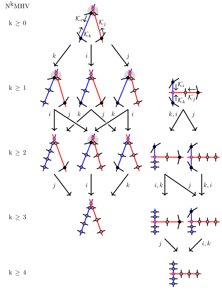
Figure 1: The twistor diagrams depicting the 14 distinct maximal codimension boundaries of two-loop $\textrm{N}^{\textrm{k}}\textrm{MHV}$ amplituhedra. See the text for more details.

We find a total of 14 topologically distinct maximal codimension configurations at two loops, which are summarized in Fig. 1. The figure emphasizes the fact that all 14 varieties of $\mathcal{L}$-boundaries can be obtained by some sequence of helicity-increasing operations $\mathcal{K}$ (defined in Sec. 5.2 of Prlina:2017azl ) acting on just two primitive diagrams, one at MHV level and one at NMHV level. The entirety of this figure should be thought of as the two-loop $d=8$ analog of the one-loop $d=4$ column of Fig. 2 of that reference. In the figure, an arrow labeled by $i$ indicates that the diagram at the end of the arrow can be obtained by acting with $\mathcal{K}_{i}$ on the diagram at the beginning of the arrow. An arrow carries two labels if the result of acting with two different instances of $\mathcal{K}$ gives topologically equivalent diagrams, in which case only the diagram corresponding to the first label on the arrow is shown. Note that for each diagram, the minimal value of k precisely matches the number of non-MHV intersections.

3.1 Resolutions

In each of the 14 twistor diagrams shown in Fig. 1, the configuration manifestly exhibits a total of $2n_{\textrm{filled}}+n_{\textrm{empty}}=8$ on-shell conditions, where $n_{\textrm{filled}}$ is the number of filled nodes and $n_{\textrm{empty}}$ is the number of empty nodes (including, in each diagram, the node at the intersection of the two loop momenta).

However, on certain sufficiently high codimension boundaries, additional on-shell conditions can be implied by the others and are therefore “accidentally” satisfied. This phenomenon occurs for the four twistor diagrams in Fig. 1 that have been drawn with a filled node at the point $Z_{i}$ and two empty nodes in close proximity (grouped in a faint gray circle in Fig. 1), representing the four on-shell conditions

$$\langle\mathcal{L}^{(1)}\,i{-}1\,i\rangle=\langle\mathcal{L}^{(1)}\,i\,i{+}1\rangle=\langle\mathcal{L}^{(2)}\,i\,i{+}1\rangle=\langle\mathcal{L}^{(1)}\,\mathcal{L}^{(2)}\rangle=0\,.$$ (12)

The first three conditions are satisfied by $\mathcal{L}^{(1)}=(Z_{i},A)$ and $\mathcal{L}^{(2)}=(\alpha Z_{i}+(1-\alpha)Z_{i+1},B)$ for any points $A$, $B$. Then, for generic $A$ and $B$, the fourth condition in Eq. (12) implies that $\alpha=1$, so the line $\mathcal{L}^{(2)}$ is forced to pass through the point $Z_{i}$. Therefore, configurations of this type satisfy the additional on-shell condition $\langle\mathcal{L}^{(2)}\,i{-}1\,i\rangle=0$.

This phenomenon reflects the fact that in general, the on-shell conditions satisfied by a given configuration are not independent: some of them may be implied by the others. In Dennen:2016mdk it was found that solving the Landau equations for boundaries of this type was rather subtle, and required first identifying a suitable minimal subset of independent on-shell conditions, a process called resolution. It was suggested that a resolution must satisfy two criteria: (1) the chosen subset of on-shell conditions must imply the full set of conditions satisfied for generic (projected) external data, and (2) the Landau diagram corresponding to the subset must be planar.

The example considered above describes a configuration that satisfies five on-shell conditions, the four shown in Eq. (12) and also $\langle\mathcal{L}^{(2)}\,i{-}1\,i\rangle=0$. There are four possible resolutions that satisfy criterion (1): we can simply omit any one of the conditions except for $\langle\mathcal{L}^{(1)}\,\mathcal{L}^{(2)}\rangle=0$. However not all four choices will satisfy criterion (2), depending on the points $A$ and $B$. For the four configurations appearing in Fig. 1 that require resolution, there are in each case precisely two valid resolutions: we can omit either $\langle\mathcal{L}^{(2)}\,i{-}1\,i\rangle=0$ (as was done in Eq. (12)), or we can omit $\langle\mathcal{L}^{(1)}\,i\,i{+}1\rangle=0$.

In Fig. 1 we have chosen to always draw a resolved configuration in the four cases where it is necessary. However, in order to avoid clutter we do not draw both resolutions unless they give rise to inequivalent diagrams. There are at least three reasons for preferring the resolved configurations. First of all, it becomes somewhat less clear how to see the action of the three graph operators $\mathcal{K}$, $\mathcal{U}$ and $\mathcal{R}$ on an unresolved configuration. Also, the need for resolution is an accident that occurs only when both loop momenta lie in the low-k branch of solutions to their respective on-shell conditions (or, by parity symmetry, when they both lie in the high-k branch). If one of them lies in the low-k branch and the other lies in the high-k branch, then for generic (projected) external data only the resolved configuration(s) exist; the “extra” on-shell condition would place restrictions on the external data. Finally, when we turn our attention to finding Landau singularities in Sec. 5, we will always want to work with resolved diagrams since these give us the independent sets of on-shell conditions for which we will need to solve the Landau equations Dennen:2016mdk .

3.2 Relaxations

All lower-codimension $\mathcal{L}$-boundaries are relaxations: they can be generated by releasing one or more of the seven on-shell conditions (excepting $\langle\mathcal{L}^{(1)}\,\mathcal{L}^{(2)}\rangle=0$, which we always preserve) satisfied on the maximal boundaries. Boundaries of this type can be generated by acting on the twistor diagrams in Fig. 1 with sequences of the graph operators $\mathcal{U}$ and $\mathcal{R}$. In this way one could imagine uplifting the figure to a three-dimensional generalization of Fig. 2 of Prlina:2017azl , with the top layer being a copy of Fig. 1 showing the maximal codimension boundaries ($d=8$), the next layer showing those with $d=7$, etc. One novelty compared to the one-loop analysis of Prlina:2017azl is that starting at two loops the relaxation of a boundary is not necessarily still a boundary — this will only be the case if the Landau diagram of the relaxation continues to be planar.

Rather than attempting to draw the aforementioned web of interconnected boundaries in a single figure, we summarize our results in terms of the corresponding Landau diagrams in Tabs. 1–5 grouped according to the minimum helicity for which the configuration is valid, i.e. the minimum k for which $\mathcal{A}_{n,\textrm{k},2}$ has boundaries of the type shown in the corresponding twistor diagram. Because the maximal codimension singularities have $d_{1}+d_{2}=7$, the corresponding Landau diagrams always have the topology of a planar pentagon-box.

	Twistor Diagram	Landau Diagram
(a)

Table 1: The twistor and Landau diagram describing a type (the unique type, for $\textrm{k}=0$) of resolved maximal codimension boundary of $\textrm{N}^{\textrm{k}\geq 0}\textrm{MHV}$ amplituhedra.

As mentioned above the lower codimension singularities can be obtained by acting on the twistor diagrams with sequences of $\mathcal{U}$ and $\mathcal{R}$ operators. As discussed in Sec 5.2 of Prlina:2017azl , at one loop these operators generate relaxations that respectively preserve or increase, but can never decrease, the minimum helicity for which a configuration is valid. There is however a subtlety with the $\mathcal{U}$ operator at two loops. Recall that $\mathcal{U}_{i,\mp}$ is the “unpinning” operator which acts on a loop momentum $\mathcal{L}$ passing through some point $Z_{i}$ by relaxing the on-shell condition $\langle\mathcal{L}\,i\,i{\pm}1\rangle=0$. This can have the effect of turning what was a manifest intersection between the two loop momenta into a non-manifest intersection, which requires increasing the minimum helicity by 1.

	Twistor Diagram	Landau Diagram
(a)
(b)
(c)
(d)

Table 2: The twistor and Landau diagrams describing types of (resolved, in (a) and (c)) maximal codimension boundaries of $\textrm{N}^{\textrm{k}\geq 1}\textrm{MHV}$ amplituhedra.

	Twistor Diagram	Landau Diagram
(a)
(b)
(c)
(d)
(e)

Table 3: The twistor and Landau diagrams describing types of (resolved, in (b)) maximal codimension boundaries of $\textrm{N}^{\textrm{k}\geq 2}\textrm{MHV}$ amplituhedra.

In the tables we have introduced a new graphical notation in order to account for this phenomenon: a propagator with a black dot denotes an on-shell condition that cannot be relaxed without increasing the minimum helicity for which the configuration is valid. (We also always draw a black dot on the $\langle\mathcal{L}^{(1)}\,\mathcal{L}^{(2)}\rangle$ propagator, as a reminder that we never want to relax it.) Consider for example the twistor diagram in Tab. 1(a). The two loop momenta manifestly intersect at the point $Z_{i}$ as explained in the previous section, but this will no longer be the case if we act on this twistor diagram with $\mathcal{U}_{i,-}$. Instead, the configuration would become NMHV rather than MHV (in fact, it would become a relaxation of Tab. 2(d), up to relabeling). For this reason we draw a black dot on the $(i\,i{+}1)$ propagator on the pentagon in the Landau diagram of Tab. 1(a).

	Twistor Diagram	Landau Diagram
(a)
(b)
(c)

Table 4: The twistor and Landau diagrams describing types of maximal codimension boundaries of $\textrm{N}^{\textrm{k}\geq 3}\textrm{MHV}$ amplituhedra.

3.3 Closing Comments

In summary, to get the full list of Landau diagrams at helicity $\textrm{k}=0,1,2,3,4$, one must therefore consider all of the Landau diagrams in Tables. 1 through 5, respectively, together with the diagrams generated therefrom by collapsing any subset of undotted propagators.

In Fig. 1 and in the tables we have chosen to always draw the loop momentum satisfying $d_{1}=4$ in blue and the one satisfying $d_{2}=3$ in red, but of course the amplituhedron is symmetric under the exchange of any $\mathcal{L}$’s so in each case both assignments $\mathcal{L}^{(1)}$, $\mathcal{L}^{(2)}$ and $\mathcal{L}^{(2)}$, $\mathcal{L}^{(1)}$ describe valid boundaries.

The Landau diagrams in Tables 1–5 are always drawn with the understanding that all indicated labels are cyclically ordered: $i<i^{\prime}<j<j^{\prime}<j^{\prime\prime}<k<k^{\prime}<k^{\prime\prime}<i$ (mod $n$). However, the ordering of intersections along the red or blue loop momentum lines carries no significance. Therefore, as described in Sec. 5.1 of Prlina:2017azl , there is a second type of ambiguity between the two classes of diagrams. For example, the twistor diagram in Tab. 2(a) is agnostic about the cyclic ordering of $i$, $k$, and $k^{\prime}$; the two independent choices lead to the Landau diagram shown in the table or to its mirror image. In all of the tables we use primes (and, when necessary, also double primes) to indicate pairs (or triplets) of nodes that can be exchanged, as far as the twistor diagram is concerned. Sometimes, as in the example Tab. 2(a) just considered, an exchange generates a Landau diagram of the same topology, but in other cases it can generate a new topology. For example, exchanging $k$ and $k^{\prime}$ in the twistor diagram of Tab. 2(b) generates the new Landau diagram

$$\begin{gathered}\includegraphics{./figures/ld_n1mhv_c2.pdf}\end{gathered}\,,$$ (14)

where it is to be understood that $i<j<k^{\prime}<k<i$.

	Twistor Diagram	Landau Diagram
(a)

Table 5: The twistor and Landau diagram describing a type of maximal codimension boundary of $\textrm{N}^{\textrm{k}\geq 4}\textrm{MHV}$ amplituhedra.

Let us also note that although when interpreted literally as configurations of intersecting lines in $\mathbb{P}^{3}$ most twistor diagrams only depict the low-k branch of solutions to a given set of on-shell conditions, it is clear that additional, higher-k boundaries can be generated by replacing one or both of the $\mathcal{L}$’s with their parity conjugates. The twistor diagrams appearing in Fig. 1 and in the five tables can therefore each be thought of as representing four different types of boundaries corresponding to the same Landau diagram.

Finally, we detail, in Appendix B, how a partial edge-to-node duality maps between the twistor diagrams on the left and the Landau diagrams on the right of these tables, when the two diagrams are treated as graphs. On the one hand, it is not surprising that there exists some map between these two classes of graphs, since both are designed to encode the same information. On the other hand, it is intriguing that there is a straightforward map between a generic Landau diagram and the minimum-helicity solution to the on-shell conditions of said diagram in the very particular choice of loop momentum twistor coordinates. This observation is also reminiscent of the map from Feynman integrals to their duals that aided in exploring the dual conformal invariance of SYM theory amplitudes Drummond:2006rz ; Alday:2007hr ; Drummond:2008vq but here, enticingly, this partial edge-to-node map is well-defined even on nonplanar graphs.

4 The Connection With On-Shell Diagrams

So far, we have seen that to each boundary of an amplituhedron one can associate a Landau diagram which encodes information about the singularities of the associated amplitude. In this section we explore the connection between Landau diagrams and a class of closely related diagrams that also encode information about an amplitude’s mathematical structure: the on-shell diagrams of ArkaniHamed:2012nw . We explain and demonstrate in several examples that for a given amplitude, the information content of certain on-shell diagrams matches the combined information content in the amplituherdon and Landau diagrams. Except possibly for cases of the type discussed in the paragraph following Eq. (36), we expect our arguments to also hold for amplitudes at higher loop order and higher helicity.

One reason to shift focus to on-shell diagrams is that anything that can be formulated in terms of the on-shell diagrams discussed here potentially generalizes to more general quantum field theories including less supersymmetric theories as well as the full, non-planar super-Yang–Mills theory. The major difference is that in the planar theory, the relevant Landau diagrams can, in principle, be read off from the boundaries of $\mathcal{A}_{n,\textrm{k},L}$ for arbitrary $n$, k, and $L$, while in the non-planar sector there is currently no known supplier of this list of diagrams. Nevertheless, assuming one has a way to generate a representation for a given non-planar amplitude in terms of Feynman integrals, all of the techniques discussed in this section apply equally well to those non-planar integrals.

Putting that ambitious motivation aside, in the rest of this section we stick to planar SYM theory and show in several examples that a given Landau diagram encodes a singularity of an $\textrm{N}^{\textrm{k}}\textrm{MHV}$ amplitude only if the diagram can be decorated in such a way that it becomes an on-shell diagram associated with an $\textrm{N}^{\textrm{k}}\textrm{MHV}$ amplitude. We begin with a brief review of on-shell diagrams.

4.1 On-Shell Diagrams

An on-shell diagram, as introduced in ArkaniHamed:2012nw , is a connected trivalent graph with each node having one of two distinct decorations, traditionally denoted by coloring them black or white. In the application to scattering amplitudes, each edge of the diagram represents an on-shell condition (just like in a Landau diagram) and each black (white) node corresponds to a three-point MHV ($\overline{\rm MHV}$) tree-level superamplitude. A straightforward generalization allows nodes of higher degree which represent higher-point tree-level superamplitudes. These we depict by a shaded node.

We refer the reader to ArkaniHamed:2012nw for details, recalling here only a few basic facts. A tree-level superamplitude of Grassmann weight $\kappa$ is a rational function of (projected) external data that is a homogeneous polynomial of degree $4\kappa$ in certain Grassmann variables (the fermionic partners of the momentum twistors $Z_{i}$). Three-point MHV and $\overline{\rm MHV}$ amplitudes respectively have $\kappa=2$ and $\kappa=1$ while for $n>3$ an $n$-point amplitude with helicity k has $\kappa=\textrm{k}+2$. To each on-shell diagram there is an associated differential form that is obtained by first multiplying together the tree-level superamplitudes represented by each of the diagram’s nodes, and then sewing them together according to a set of simple rules that involve integrating over four Grassmann variables for each internal edge (propagator) in the diagram. Such forms are the values of the residue of the amplitude’s integrand at specific loci in loop momentum space.

Consider an on-shell diagram $\delta$. Let $\iota$ be the number of internal edges of $\delta$, and for each node $\nu$ let $\kappa_{\nu}$ be the Grassmann weight of the tree-level superamplitude at $\nu$. As a result of the rules just reviewed, the total Grassmann weight of $\delta$ is

$$\kappa_{\delta}=\sum_{\nu}\kappa_{\nu}-\iota\,,$$ (15)

and the total helicity is $\textrm{k}_{\delta}=\kappa_{\delta}-2$.

To assign a coloring to a Landau diagram depicting some set of on-shell conditions means to assign to each trivalent node in the diagram either a white or black coloring, and to assign to each node $\nu$ of degree $n>3$ some helicity $\textrm{k}_{\nu}=\kappa_{\nu}-2\in\{0,\ldots,n-4\}$. Since $\iota$ is fixed by the propagator structure of the diagram, and each $\kappa_{\nu}$ is positive, it is clear from Eq. (15) that the minimal Grassmann weight of a given Landau diagram results from coloring all trivalent nodes white and from assigning all nodes of higher degree to be MHV ($\kappa_{\nu}=2$). In this way we see that the Grassmann weight of an arbitrary coloring of a given Landau diagram is bounded below by

$$\kappa\geq\kappa_{\textrm{min}}=n_{\textrm{tri}}+2n_{\textrm{high}}-\iota\,,$$ (16)

where $n_{\textrm{tri}}$ is the number of trivalent nodes and $n_{\textrm{high}}$ is the number of nodes of degree higher than three. This implies a minimal helicity sector $k_{\textrm{min}}=\kappa_{\textrm{min}}-2$ for which the Landau diagram can be relevant.

If a diagram has $n_{\textrm{tri}}$ trivalent indices, there are $2^{n_{\textrm{tri}}}$ colorings of the trivalent nodes, but in general some of these may lead to on-shell diagrams that evaluate to zero. In practice we count the number of permissible colorings of a diagram by solving the on-shell conditions implied by the diagram and mapping each resulting solution to a specific coloring (see ArkaniHamed:2012nw ). As discussed in ArkaniHamed:2010gh , solving a set of on-shell conditions in momentum twistor space amounts to solving a Schubert problem. At one loop these problems have in general two solutions, while for an $L$-loop Landau diagram we would in general expect $2^{L}$ branches of solutions. Given a solution to a Schubert problem in momentum twistor space, it is straightforward to check if a given trivalent node is MHV or $\overline{\rm MHV}$ by considering the rank of the three momentum-twistor lines at the node. For an MHV node, the three twistors have full rank, while for an $\overline{\rm MHV}$ node the rank is less than full. This process is illustrated explicitly in several examples in the following section.

In summary, we have reviewed that a given Landau diagram encodes a set of on-shell conditions, and the various branches of solutions to those conditions correspond in general to different minimum helicity sectors. The permissible colorings of a Landau diagram are in one-one correspondence with those branches, and the Grassmann weight $\kappa$ of each such Landau-turned-on-shell diagram is related to the minimum helicity sector k of the corresponding solution via $\kappa=\textrm{k}+2$.

This observation provides an alternative way to phrase the Landau-equation-based algorithm we employ to identify singularities of amplitudes, compared for example to the way it is phrased in the conclusion of Dennen:2016mdk or in Sec. 2.5 of Prlina:2017azl . For one thing, it means we can identify a singularity of a Landau diagram as a singularity of $\textrm{N}^{\textrm{k}}\textrm{MHV}$ amplitudes only if the diagram admits a coloring with total helicity k (equivalently, Grassmann weight $\textrm{k}+2$). More specifically, when first solving the on-shell conditions (a subset of the Landau equations) for a given Landau diagram, each solution directly indicates, via the test reviewed in the previous paragraph, the helicity sector for which the singularity associated to that solution is relevant. In the on-shell diagram approach this step is the analog in the amplituhedron approach of identifying the values of k for which the momentum twistor solution lies on the boundary of the $\textrm{N}^{\textrm{k}}\textrm{MHV}$ amplituhedron. In the amplituhedron-based approach, there is potential for confusion because solving the Kirchhoff conditions (the remaining Landau equations) can lead to solutions for loop momenta that lie outside the $\textrm{N}^{\textrm{k}}\textrm{MHV}$ amplituhedron. The on-shell diagram approach bypasses this confusion because the Kirchhoff conditions only further localize a loop momentum solution whose helicity sector has already been identified.

4.2 Examples at One and Two Loops

We now consider several examples in order to emphasize the following point:

$$\begin{array}[]{l}\textrm{A Landau diagram contributes singularities to an $\textrm{N}^{\textrm{k}}\textrm{MHV}$ amplitude }\\ \textrm{only if the diagram permits a coloring with total Grassmann weight $\textrm{k}+2$. }\end{array}$$ (19)

For each of our examples, we also list the values of the loop momenta corresponding to the colorings of the correct Grassmann weight. For the one-loop examples the same information can be read off from Tab. 1 of Prlina:2017azl . We will show how the on-shell diagram and amplituhedron-based methods work in tandem to quickly identify the helicity sector for which a given solution to the set of on-shell conditions is relevant.

One-loop Two-mass Easy Box

The on-shell conditions

$$\langle\mathcal{L}\,i{-}1\,i\rangle=\langle\mathcal{L}\,i\,i{+}1\rangle=\langle\mathcal{L}\,j{-}1\,j\rangle=\langle\mathcal{L}\,j\,j{+}1\rangle=0$$ (20)

admit two solutions, called branches (12) and (13) in Prlina:2017azl . In Tab. 6 we pair the momentum twistor representation of each solution with the associated on-shell diagram, i.e. colored Landau diagram. Having this information accessible will prove useful when considering two loops.

In Tab. 6(a) the minimum Grassmann weight is computed according to Eq. (16) and found to be

$$\kappa_{\textrm{min}}=\underbrace{1+1}_{\textrm{white}}+\underbrace{2+2}_{\textrm{higher}}-4=2$$ (21)

so that it is an MHV ($\textrm{k}=2-2=0$) coloring.

In Tab. 6(b) the minimum Grassmann weight is

$$\kappa_{\textrm{min}}=\underbrace{2+2}_{\textrm{black}}+\underbrace{2+2}_{\textrm{higher}}-4=4$$ (22)

so that it is an $\textrm{N}^{2}\textrm{MHV}$ ($\textrm{k}=4-2=2$) coloring.

Let us now show how to compute the appropriate node colorings directly from the momentum twistor solutions in Tab. 6. Consider the trivalent node where external label $i$ connects to the loop. The three lines in momentum twistor space defining the trivalent node are $(i{-}1\,i)$, $(i\,i{+}1)$, and $\mathcal{L}_{*}$, where $\mathcal{L}_{*}$ is either $(i\,j)$ or $\overline{i}\cap\overline{j}$. Taking first $\mathcal{L}_{*}=(i\,j)$ , we seek the dimension of the space spanned by the three momentum-twistor lines. One way to compute this is to ask for the rank of the matrix:

$$\textrm{rank}\left(\begin{array}[]{c}(i{-}1\,i)\\ (i\,i{+}1)\\ (i\,j)\end{array}\right)=\textrm{rank}\bordermatrix{&i{-}1&i&i{+}1&j\cr&1&0&0&0\cr&0&1&0&0\cr&0&1&0&0\cr&0&0&1&0\cr&0&1&0&0\cr&0&0&0&1\cr}=4$$ (26)

which has maximal rank. So the node is MHV, and colored white.

In contrast, consider the other solution $\mathcal{L}_{*}=\overline{i}\cap\overline{j}$. The analogous matrix is then

$$\textrm{rank}\left(\begin{array}[]{c}(i{-}1\,i)\\ (i\,i{+}1)\\ \overline{i}\cap\overline{j}\end{array}\right)=\textrm{rank}\bordermatrix{&i{-}1&i&i{+}1\cr&1&0&0\cr&0&1&0\cr&0&1&0\cr&0&0&1\cr&\langle i\,\overline{j}\rangle&-\langle i{-}1\,\overline{j}\rangle&0\cr&0&\langle i{+}1\overline{j}\rangle&-\langle i\,\overline{j}\rangle\cr}=3$$ (30)

which does not have maximal rank. Thus the second solution is encoded in an $\overline{\rm MHV}$ node at $i$, colored black. The colorings of the node at $j$ can be computed analogously.

	Coloring	$\textrm{N}^{\textrm{k}}\textrm{MHV}$	Twistor Solution
(a)		$\textrm{k}\geq 0$	$\mathcal{L}=(i\,j)$
(b)		$\textrm{k}\geq 2$	$\mathcal{L}=\overline{i}\cap\overline{j}$

Table 6: Two colorings of the two-mass easy box. Row (a) shows the MHV coloring and momentum twistor solution to the on-shell conditions, and row (b) shows the same for the $\textrm{N}^{2}\textrm{MHV}$ solution.

	Coloring	$\textrm{N}^{\textrm{k}}\textrm{MHV}$	Twistor Solution
(a)		$\textrm{k}\geq 1$	$\mathcal{L}=(i\,j\,j{+}1)\cap(i\,k\,k{+}1)$
(b)		$\textrm{k}\geq 2$	$\begin{array}[]{c}\mathcal{L}=(A\,B)\\ A=(j\,j{+}1)\cap\overline{i}\\ B=(k\,k{+}1)\cap\overline{i}\end{array}$

Table 7: Two colorings of the three-mass box. Row (a) shows the NMHV coloring and momentum twistor solution to the on-shell conditions, and row (b) shows the same for the $\textrm{N}^{2}\textrm{MHV}$ solution.

One-loop Three-mass Box

We perform the same exercise for the three-mass box on-shell conditions

$$\langle\mathcal{L}\,i{-}1\,i\rangle=\langle\mathcal{L}\,i\,i{+}1\rangle=\langle\mathcal{L}\,j\,j{+}1\rangle=\langle\mathcal{L}\,k\,k{+}1\rangle=0\,.$$ (31)

The solutions of the on-shell conditions are matched to the two on-shell diagram colorings in Tab. 7, and the corresponding minimum Grassmann weights are computed using Eq. (16). The colorings are also directly calculable from the momentum twistor solutions as in the previous two-mass easy box example. The three-mass box is worth pointing out because in this case neither coloring is MHV, in contrast to the previous example.

Two-loop Pentagon-box

We can recycle our knowledge of one-loop solutions to determine the helicity sectors to which a given two-loop Landau diagram contributes its singularities. We consider the pentagon-box of Tab. 2(a) as an exemplar. We solve the pentagon-box on-shell conditions as follows. We first solve the subsystem of four propagators that depend on only $\mathcal{L}^{(2)}$:

$$\langle\mathcal{L}^{(2)}\,i{-}1\,i\rangle=\langle\mathcal{L}^{(2)}\,i\,i{+}1\rangle=\langle\mathcal{L}^{(2)}\,k\,k{+}1\rangle=\langle\mathcal{L}^{(2)}\,k^{\prime}\,k^{\prime}{+}1\rangle=0$$ (32)

using either of the two three-mass box solutions shown in Tab. 7, after an appropriate exchange of the external labels in order to match to Eq. (32). This means there are two branches of colorings: one were the trivalent node at $i$ is white, and one where it is black. The two corresponding solutions $\mathcal{L}^{(2)}_{*}$ are shown in the first row of Tab. 8. For each choice of $\mathcal{L}^{(2)}_{*}$ we then solve the remaining four on-shell conditions

$$\langle\mathcal{L}^{(1)}\,i\,i{+}1\rangle=\langle\mathcal{L}^{(1)}\,j{-}1\,j\rangle=\langle\mathcal{L}^{(1)}\,j\,j{+}1\rangle=\langle\mathcal{L}^{(1)}\,\mathcal{L}^{(2)}_{*}\rangle\,.$$ (33)

These four conditions constitute a two-mass easy box problem, so we can utilize Tab. 6 to identify the two solutions $\mathcal{L}_{*}^{(1)}$, which color the trivalent nodes of the box either both white or both black. These two solutions are tabulated in the first column of Tab. 8. Altogether the table shows a grid containing a total of four distinct solutions, and the four associated distinct colorings. From this analysis we conclude that only the solution

$$\mathcal{L}^{(2)}_{*,1}=(i\,k\,k{+}1)\cap(i\,k^{\prime}\,k^{\prime}{+}1)\,,\ \mathcal{L}^{(1)}_{*,1}=(j\,i\,i{+}1)\cap(j\,\mathcal{L}_{*,1}^{(2)})=(i\,j)$$ (34)

shown in the top left of Tab. 8 is relevant to the NMHV sector. This means that when we turn in the following section to the problem of finding singularities of NMHV amplitudes by solving the Landau equations, we can disregard the other three solutions. Were we to attempt an amplituhedron-based answer to this same question, we would find that the other solutions to the on-shell conditions do not lie on a boundary of $\mathcal{A}_{n,1,2}$.

$\mathcal{L}^{(1)}_{*}\backslash\mathcal{L}^{(2)}_{*}$	$(i\,k\,k{+}1)\cap(i\,k^{\prime}\,k^{\prime}{+}1)$	$\begin{array}[]{c}((k\,k{+}1)\cap\overline{i}\,(k^{\prime}\,k^{\prime}{+}1)\cap\overline{i})\\ \end{array}$
$(i\,j)$
	$\textrm{k}\geq 1$	$\textrm{k}\geq 2$
$\bar{i}\cap\bar{j}$
	$\textrm{k}\geq 3$	$\textrm{k}\geq 4$

Table 8: All permissible colorings of the trivalent nodes of the two-loop pentagon-box Landau diagram from Tab. 2(a). The first row shows the two possible solutions to the three-mass on-shell conditions (Eq. (32)) satisfied by $\mathcal{L}^{(2)}$, the loop momentum in the pentagon. The first column shows the two possible solutions to the two-mass easy on-shell conditions (Eq. (33)) satisfied by $\mathcal{L}^{(1)}$, the loop momentum in the box. The cell at the intersection of a row and a column is the colored Landau diagram that results from the two solutions. Also indicated in each cell is the minimum helicity sector of the colored Landau diagram, which is achieved only if the gray nodes are taken to be MHV.

General Two-Loop Pentagon-Boxes

By using the same simple counting arguments applied to the results in Tables 1–5, it is a straightforward exercise to show that

• the set of Landau diagrams corresponding to the maximal codimension boundaries of $\mathcal{A}_{n,\textrm{k},2}$ and

• the set of on-shell diagrams of pentagon-box topology that admit an $\textrm{N}^{\textrm{k}}\textrm{MHV}$ coloring

are the same. Specifically, the second set may be constructed by starting with a pentagon-box diagram with no external edges or coloring, then placing all possible combinations of massive and massless edges on nodes of the diagram in all possible ways, and finally enumerating all colorings of the resulting Landau diagrams to identify the minimum possible value of k.

5 Landau Singularities of Two-Loop NMHV Amplitudes

Finally we come to step 2 of the algorithm summarized in Sec. 2.5 of Prlina:2017azl : in order to determine the locations of Landau singularities of the two-loop $\textrm{N}^{\textrm{k}}\textrm{MHV}$ amplitude in SYM theory, we must identify, for each $\mathcal{L}$-boundary of $\mathcal{A}_{n,\textrm{k},2}$ tabulated in Sec. 3, the codimension-one loci (if there are any) in $\operatorname{Conf}_{n}(\mathbb{P}^{3})$ on which the corresponding Landau equations admit nontrivial solutions.

The ultimate aim of this project has been to derive (or at least to conjecture) symbol alphabets for two-loop amplitudes. However, as discussed in Sec. 7 of Prlina:2017azl , guessing a symbol alphabet from a list of singularity loci can require a nontrivial extrapolation. At one loop the extrapolation is straightforward for all Landau diagrams except the four-mass box.

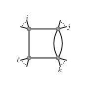
$\sim$

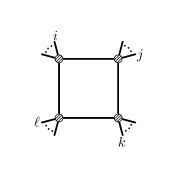
Figure 2: The Landau equations of a Landau diagram containing a bubble are identical to the equations of a Landau diagram with one propagator of the bubble removed. The two-loop four-mass bubble-box on the left is the only Landau diagram with a four-mass box contributing to the branch points of the NMHV amplitude. It has the same well-known branch points as the one-loop four-mass box on the right.

At two loops, four-mass box subdiagrams become prevalent starting at $\textrm{k}=2$, where they appear in the maximal codimension Landau diagram shown in Tab. 2(e), as well as in many of the relaxations of the other Landau diagrams in Tab. 2. At $\textrm{k}=1$ there is a single four-mass bubble-box Landau diagram, Fig. 2, relevant to two-loop NMHV amplitudes. As shown in the Appendix of Dennen:2016mdk , Landau diagrams containing bubble subdiagrams are equivalent to the same diagram with one of the propagators of the bubble removed. So we expect the one-loop four-mass box singularity to reappear as a singularity of the two-loop NMHV amplitude. Though we are only guaranteed from this analysis that the singularities match, we can throw caution to the wind and conjecture that the same symbol entries that appear in the one-loop four-mass box integral appear also in two-loop NMHV amplitudes. Of note here: the four-mass box has support starting at $\textrm{k}=2$, so there is shared singularity structure between the two-loop NMHV and one-loop $\textrm{N}^{2}\textrm{MHV}$ amplitudes.

Having dealt with this single caveat, we restrict our analysis to the remaining NMHV singularities, where we may hope that our approach allows us to read off symbol alphabets directly from lists of singularity loci.

5.1 Computational Approaches

Sec. 2.4 of Prlina:2017azl reviews the Landau equations and Sec. 6 of that reference details the process of solving them in several one-loop examples. Beyond one loop, one approach for seeking solutions is to perform the analysis “one loop at a time”, by considering each one-loop subdiagram and writing down the constraints on the values of other loop and external momenta imposed by the on-shell and Kirchhoff conditions of the subdiagram. After taking the union of those constraints, one may conclude that a solution exists for generic external data, or that the solution exists only when the external data satisfy some set of equations. Solutions of the former type were associated with the infrared singularities of an amplitude in Dennen:2015bet , and solutions of the latter type indicate branch points of the amplitude when they live on codimension-one loci in $\operatorname{Conf}_{n}(\mathbb{P}^{3})$.

Here we recall a few basic facts about this loop-by-loop approach, which has been carried out for several cases in Dennen:2015bet ; Dennen:2016mdk .

First, as mentioned above, one edge of a bubble subdiagram can always be removed without affecting Landau analysis.

Second, as shown in the Appendix of Dennen:2016mdk , a generic triangle subdiagram has seven different branches of solutions that should be considered separately. All of the solutions demand that the squared sum of momenta on “external” edges attached to at least one of the triangle’s corners vanish, and the seven branches of solutions are classified according to the number of null corners. There are three branches of “codimension-one” solutions (any one of the three corners vanishing), three branches of “codimension two” (any two of the three corners vanishing) and one of “codimension three” (all corners vanishing). In a Landau diagram analysis, it will often be the case that one of a triangle’s corners is null by fiat; in this case, the solution space will be reduced. For example, a “two-mass” triangle subdiagram has only one codimension-one solution. In the examples we detail in Sec. 5.2, all triangle subdiagrams we describe are of this two-mass variety.

Finally, the Kirchhoff conditions associated to a box subdiagram constitute four homogeneous equations on four Feynman parameters, so the existence of nontrivial solutions requires the vanishing of a certain four-by-four determinant called the Kirchhoff constraint for the box. The Kirchhoff constraints for the four different cases of box diagrams are summarized in Eqns. (2.7) through (2.11) of Dennen:2015bet .

It is worth noting one detail regarding the “one loop at a time” approach. Because the method starts by enumerating the constraints imposed by the existence of nontrivial solutions to the Landau equations of each subdiagram, it will miss the solutions which set all Feynman parameters corresponding to some one-loop subdiagram to zero. However, Landau singularities obtained this way will always be those already present at lower loop order. So the “one loop at a time” approach neglects no novel branch points. We comment on a specific example of this phenomenon in the next section.

Let us also describe a conceptually simpler but computationally less effective alternative approach which we have used as a cross-check on our results. For a given branch of solutions to a set of on-shell conditions, or equivalently, for a given on-shell diagram, one can reduce the Landau equations “all at once” to see whether they impose codimension-one constraints on the external data. This approach is of course usually feasible only with the aid of a computer algebra system such as Mathematica. It also lends itself well to numerical experimentation: one can probe the presence or absence of a putative singularity at some locus $a=0$ by generating random numeric values for the external data except for one free parameter $z$, and then reducing the Landau equations to see if the existence of nontrivial solutions forces $z$ to take a value that sets $a=0$.

Before proceeding to the examples and results, let us address the question: how do we confirm that we have detected all singularities? Starting from the maximal codimension boundaries of the NMHV amplituhedron shown in Tab. 2, we determine all corresponding Landau diagrams keeping in mind the ambiguity mentioned in Sec. 3.3. From there it is straightforward to produce all possible relaxed Landau diagrams. And from the diagrams we compute the singularities using the “one loop at a time” approach outlined above. Once we have a list of potential singularities, we turn to the “all at once” numerical probing. Doing so we directly confirm on a diagram-by-diagram basis not only that the set of singularities is correct, but also that there are no additional singularities. We have performed these steps to confirm the NMHV singularities presented in Sec. 5.3.

We will focus only on Landau diagrams that have minimally-NMHV coloring, as defined in Sec. 4.1, or equivalently, diagrams that come from a boundary of a two-loop NMHV amplituhedron. A priori, we cannot dismiss the possibility that a minimally-MHV diagram may have novel singularities coming from an NMHV branch of solutions, but we have explicitly checked that this does not occur in the two-loop NMHV amplitudes we consider here. We will demonstrate our “one loop at a time” approach to solving Landau equations on an example in the next section, and then proceed to list the full set of singularities in Sec. 5.3.

5.2 A Sample Two-Loop Diagram

We now turn to the Landau analysis of the boundaries displayed in Tab. 2. The analysis is very similar to that of the many examples that have been considered in Dennen:2015bet ; Dennen:2016mdk , to which we refer the reader for additional details. Therefore we only carry out the analysis in detail for the case of Tab. 2(a), and summarize all of the results in the following section.

At maximal codimension the on-shell conditions encapsulated in the Landau diagram of Tab. 2(a) are shown in Eqns. (32) and (33). These have a total of four discrete solutions, as summarized in Tab. 8, but the only one relevant at NMHV order is the one displayed in Eq. (34). The Landau equations (specifically, the Kirchhoff constraint for the box subdiagram defined by Eq. (33)) admit a solution only if Dennen:2015bet

$$\langle j(j{-}1\,j{+}1)(i\,i{+}1)\,\mathcal{L}^{(2)}_{*}\rangle=0\,.$$ (35)

Substituting in the lower-helicity solution $\mathcal{L}^{(2)}_{*,1}$ and simplifying turns the constraint into

$$\langle i\,\overline{j}\rangle\langle i\,(i{+}1\,j)\,(k\,k{+}1)\,(k^{\prime}\,k^{\prime}{+}1)\rangle=0\,.$$ (36)

Now we must address a subtlety of the result (36) that is analogous to the one encountered for the maximal codimension MHV configuration under Eq. (3.29) of Dennen:2016mdk . Like in that case, the eight-propagator Landau diagram under consideration here, shown in Tab. 2(a), corresponds to a resolution of a configuration that actually satisfies nine on-shell conditions, as reviewed in Sec. 3.1. It was proposed in Dennen:2016mdk that we should trust the resulting Landau analysis only to the extent that the eight on-shell conditions imply the ninth for generic external data. Let us note that if we put $\langle\mathcal{L}^{(1)}\,\mathcal{L}^{(2)}\rangle=0$ aside for a moment, the NMHV solution to the seven other on-shell conditions is

$$\mathcal{L}^{(2)}=(i\,k\,k{+}1)\cap(i\,k^{\prime}\,k^{\prime}{+}1)\,,\qquad\mathcal{L}^{(1)}=(\alpha Z_{i}+(1-\alpha)Z_{i+1},Z_{j})\,,$$ (37)

from which we find

$$\langle\mathcal{L}^{(1)}\,\mathcal{L}^{(2)}\rangle=(1-\alpha)\langle i(i{+}1\,j)(k\,k{+}1)(k^{\prime}\,k^{\prime}{+}1)\rangle\,.$$ (38)

Therefore the conclusion that $\alpha=1$, and hence that the ninth condition $\langle\mathcal{L}^{(1)}\,i{-}1\,i\rangle=0$ is also satisfied, actually only follows if $\langle i(i{+}1\,j)(k\,k{+}1)(k^{\prime}\,k^{\prime}{+}1)\rangle\neq 0$. This observation introduces controversy about whether the second quantity on the left-hand side of Eq. (36) is a valid singularity. However, note that from the on-shell diagram point of view there is no apparent reason why this singularity should be excluded, since the diagram can be assigned a valid NMHV coloring as shown in Tab. 8. Absent a rigorous argument resolving the matter, we remain agnostic about the status of this singularity.

It is easy to see that another solution to the Landau equations with $\mathcal{L}^{(1)}=(i\,j)$ and $\mathcal{L}^{(2)}=(i\,k\,k{+}1)\cap(i\,k^{\prime}\,k^{\prime}{+}1)$ exists if the four Feynman parameters associated to the box subdiagram are set to zero. In this case the box completely decouples and the pentagon subdiagram reduces to a three-mass box, so this branch exists if the external data satisfy the corresponding Kirchhoff constraint

$$\langle i(i{-}1\,i{+}1)(k\,k{+}1)(k^{\prime}\,k^{\prime}{+}1)\rangle=0\,.$$ (39)

This illustrates the point highlighted in the previous section that the “one loop at a time” approach can miss certain solutions to the Landau equations associated entirely with one-loop subdiagrams. As mentioned, we are only seeking new singularities, whereas Eq. (39) is already known from one loop.

Next we move on to codimension seven. There are four inequivalent relaxations, which we now discuss in turn. These relaxations result from collapsing any of the undotted propagators of Tab. 2(a). We list only the minimally-NMHV diagrams; see Fig. 3.

Relaxing $\langle\mathcal{L}^{(2)}\,i{-}1\,i\rangle=0$

leads to a double-box Landau diagram, Fig. 3(a).

There are two Kirchhoff constraints (one per box), one of which is easier to determine than the other. The easier-to-find Kirchhoff constraint comes from the box formed of the $\mathcal{L}^{(1)}$-dependent propagators (including the shared propagator). It reads

$$\langle j\,(j{-}1\,j{+}1)\,(i\,i{+}1)\,\mathcal{L}^{(2)}_{*}\rangle=0\,,$$ (40)

where we write $\mathcal{L}^{(2)}_{*}$ to emphasize the loop momentum is on-shell when all Landau equations are satisfied.

The second Kirchhoff constraint is easiest to find after solving the three $\mathcal{L}^{(1)}$-dependent on-shell conditions via $\mathcal{L}^{(1)}_{*,1}=(Z_{j},B)$, with $B=\alpha Z_{i}+(1-\alpha)Z_{i+1}$. Using this form of $\mathcal{L}^{(1)}$ in the $\mathcal{L}^{(2)}$-dependent propagators (including the shared one) results in

$$\langle\mathcal{L}^{(2)}\,i\,B\rangle=\langle\mathcal{L}^{(2)}\,k\,k{+}1\rangle=\langle\mathcal{L}^{(2)}\,k^{\prime}\,k^{\prime}{+}1\rangle=\langle\mathcal{L}^{(2)}\,j\,B\rangle=0\,,$$ (41)

which are now effectively the propagators of a three-mass box. The second Kirchhoff constraint is therefore

$$\langle B\,(i\,j)\,(k\,k{+}1)\,(k^{\prime}\,k^{\prime}{+}1)\rangle=0\,.$$ (42)

Solving the remaining on-shell and Kirchhoff constraints (recall that the three $\mathcal{L}^{(1)}$-dependent conditions were solved already) fixes

$$\mathcal{L}^{(2)}_{*,1}=(A\,k\,k{+}1)\cap(A\,k^{\prime}\,k^{\prime}{+}1)\,,\quad A=(i\,i{+}1)\cap\bar{j}\,,\quad\textrm{and}$$ (43)

$$B=(i\,i{+}1)\cap(j\,\mathcal{L}^{(2)}_{*,1})\,.$$ (44)

This constraint on $B$ turns Eq. (42) into a codimension-one constraint on the external data:

$$\langle A\,(i\,j)\,(k\,k{+}1)\,(k^{\prime}\,k^{\prime}{+}1)\rangle=0\,,\quad A=(i\,i{+}1)\cap\bar{j}\,,$$ (45)

which is a new, genuinely two-loop, singularity.

Relaxing $\langle\mathcal{L}^{(1)}\,j{-}1\,j\rangle=0$

leads to a pentagon-triangle Landau diagram, Fig. 3(b).

There is a single codimension-one branch for the triangle subdiagram since there is an on-shell line at one of its corners. This branch leads to Landau equations with a solution locus that is a Kirchhoff constraint of three-mass box type:

$$\langle i\,(i{-}1\,i{+}1)\,(k\,k{+}1)\,(k^{\prime}\,k^{\prime}{+}1)\rangle=0\,.$$ (46)

We do not focus on these already familiar singularities.

Following any codimension-two branch of the triangle subdiagram leads to Landau singularities that exist only on codimension-two loci in the space of external data, which are not of interest to us.

Following the single codimension-three branch for the triangle leads to a branch of solutions to the Landau equations that exists only if

$$\langle i\,(j\,j{+}1)\,(k\,k{+}1)\,(k^{\prime}\,k^{\prime}{+}1)\rangle=0\,,$$ (47)

which is a new type of singularity.

Relaxing $\langle\mathcal{L}^{(1)}\,i\,i{+}1\rangle=0$

leads to a pentagon-triangle Landau diagram, Fig. 3(c).

There is again a single codimension-one branch for the triangle subdiagram leading to an effective decoupling of the two loop momenta and an overall Landau constraint of the same form (up to relabeling) as Eq. (46).

Following the codimension-two branches for the triangle subdiagram uncovers constraints of codimension higher than one on the external data, which cannot sensibly be associated with branch points.

Following the codimension-three branch for the triangle subdiagram leads to the same Landau singularity as in Eq. (47) (up to relabeling).

(a)	(b)	(c)
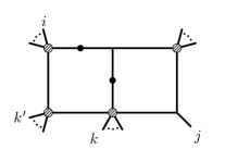
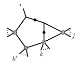
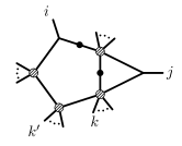
$\langle\mathcal{L}^{(2)}\,i{-}1\,i\rangle\neq 0$	$\langle\mathcal{L}^{(1)}\,j{-}1\,j\rangle\neq 0$	$\langle\mathcal{L}^{(1)}\,i\,i{+}1\rangle\neq 0$

Figure 3: These are the unique single-relaxations of Tab. 2(a) that result in NMHV Landau diagrams. The computation of the associated Landau singularities is discussed in the text.

At codimension six there are three inequivalent relaxations, shown in Fig. 4, that do not reduce the Landau diagram to an MHV one. Collapsing any of the undotted propagators of a box subdiagram in Fig. 4 results in a minimally-MHV Landau diagram, as one of the external labels would necessarily drop out. Any additional relaxations of a propagator in a triangle subdiagram of Fig. 4 will yield a bubble subdiagram, which cannot yield a new singularity as we have already emphasized.

Relaxing both $\langle\mathcal{L}^{(1)}\,i\,i{+}1\rangle$ = $\langle\mathcal{L}^{(2)}\,i{-}1\,i\rangle=0$

leads to a box-triangle Landau diagram, Fig. 4(a).

The single codimension-one branch of the triangle leads to the effective decoupling of the two loops and results in Landau singularities at Mandelstam-type loci:

$$\langle i\,i{+}1\,k\,k{+}1\rangle\langle i\,i{+}1\,k^{\prime}\,k^{\prime}{+}1\rangle\langle k\,k{+}1\,k^{\prime}\,k^{\prime}{+}1\rangle=0\,.$$ (48)

The same Landau singularities are obtained by following the codimension-two branches for the triangle.

Following the codimension-three branch for the triangle leads to the constraint

$$\langle j\,(i\,i{+}1)\,(k\,k{+}1)\,(k^{\prime}\,k^{\prime}{+}1)\rangle=0\,.$$ (49)

Relaxing both $\langle\mathcal{L}^{(2)}\,i{-}1\,i\rangle=\langle\mathcal{L}^{(1)}\,j{-}1\,j\rangle=0$

leads to a box-triangle Landau diagram, Fig. 4(b). All branches of the triangle subdiagram result in bubble-type singularities, $\langle a\,a{+}1\,b\,b{+}1\rangle$, or higher codimension constraints.

Relaxing both $\langle\mathcal{L}^{(1)}\,i\,i{+}1\rangle=\langle\mathcal{L}^{(1)}\,j{-}1\,j\rangle=0$

leads to a pentagon-bubble Landau diagram, Fig. 4(c), as discussed above and displayed in Fig. 2, with a singularity on the locus

$$\langle i\,(j\,j{+}1)\,(k\,k{+}1)\,(k^{\prime}\,k^{\prime}{+}1)\rangle=0\,.$$ (50)

(a)	(b)	(c)
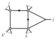
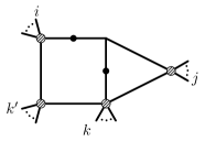
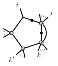
$\langle\mathcal{L}^{(2)}\,i{-}1\,i\rangle\neq 0$ $\langle\mathcal{L}^{(1)}\,i\,i{+}1\rangle\neq 0$	$\langle\mathcal{L}^{(2)}\,i{-}1\,i\rangle\neq 0$ $\langle\mathcal{L}^{(1)}\,j{-}1\,j\rangle\neq 0$	$\langle\mathcal{L}^{(1)}\,i\,i{+}1\rangle\neq 0$ $\langle\mathcal{L}^{(1)}\,j{-}1\,j\rangle\neq 0$

Figure 4: These are the unique minimally NMHV relaxations of the diagrams Fig. 3. As such, these are also double-relaxations of Tab. 2(a). Computing the associated singularities is discussed in the text. Any further relaxations of triangles yield bubble subdiagrams. In (c), relaxing either of $\langle\mathcal{L}^{(2)}\,i\,i{\pm}1\rangle=0$ yields the four-mass bubble-box of Fig. 2.

Relaxing both $\langle\mathcal{L}^{(1)}\,j{-1}\,j\rangle=\langle\mathcal{L}^{(1)}\,j\,j{+}1\rangle=0$

is displayed in Fig. 5. This case is interesting because it emphasizes the interplay between on-shell diagrams and the amplituhedron.

From the on-shell diagram perspective, this diagram naively has a minimally MHV coloring, Fig. 5(b). However the graph moves that preserve on-shell functions (particularly the “collapse and re-expand” and “bubble deletion” of Sec. 2.6 of ArkaniHamed:2012nw ) permit redrawing the coloring as a three-mass box on-shell diagram Fig. 5(c), colored in its minimal helicity manner, $\textrm{k}\geq 1$ . Since the graph moves preserve the on-shell function, the original on-shell diagram must also be minimally NMHV.

It is straightforward to check that the momentum twistor solution corresponding to this minimal coloring Fig. 5(a) is in fact a boundary of an NMHV amplituhedron, not an MHV one, and so the on-shell diagram and amplituhedron perspectives align.

For the two-loop amplitude, this diagram does not contribute new possible branch points, but this phenomenon is something to keep in mind for future studies.

(a)	(b)	(c)
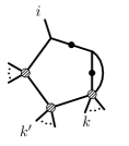
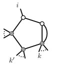
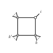
$\langle\mathcal{L}^{(1)}\,j{-}1\,j\rangle\neq 0$ $\langle\mathcal{L}^{(1)}\,j\,j{+}1\rangle\neq 0$	Minimal Coloring	After Graph Moves

Figure 5: The Landau diagram (a) appears to have a minimally MHV coloring (b). Yet the corresponding on-shell function is related by the on-shell diagram moves of ArkaniHamed:2012nw to one in the NMHV helicity sector (c).

There are no new NMHV triple relaxations, but we revisit a case discussed earlier to show how it naturally arises in this organizational scheme.

Relaxing all of $\langle\mathcal{L}^{(2)}\,i{-}1\,i\rangle=\langle\mathcal{L}^{(1)}\,i\,i{+}1\rangle=\langle\mathcal{L}^{(1)}\,j{-}1\,j\rangle=0$

leads to the bubble-box Landau diagram discussed above and displayed in Fig. 2. As mentioned above, this does not contribute a new two-loop singularity but it does indicate that two-loop NMHV amplitudes inherit the four-mass box singularity that appears at one loop only starting at $\textrm{k}=2$. Our analysis indicates this is a fairly common phenomenon: Landau diagrams for an $L$-loop $\textrm{N}^{\textrm{k}}\textrm{MHV}$ amplitude that contain bubble or triangle subdiagrams will often contain singularities that also contribute to $(L-1)$-loop $\textrm{N}^{\textrm{k}+1}\textrm{MHV}$ amplitudes.

5.3 Two-Loop NMHV Symbol Alphabets

The full set of loci in the external kinematic space $\operatorname{Conf}_{n}(\mathbb{P}^{3})$ where two-loop NMHV amplitudes have Landau singularities is obtained by carrying out the analysis of the previous section for all Landau diagrams appearing in Tabs. 1 and 2, together with all of their (still NMHV) relaxations. Among the set of singularities generated in this way are the two-loop MHV singularities that arise from the configuration shown in Tab. 1, which live on the loci

$$\begin{split}\langle a\,a{+}1\,b\,c\rangle=0\,,\\ \langle a\,a{+}1\,\overline{b}\cap\overline{c}\rangle=0\,,\end{split}$$ (51)

for arbitrary indices $a,b,c$. The set of brackets appearing on the left-hand sides of Eq. (51) correspond exactly to the set of symbol letters of two-loop MHV amplitudes originally found in CaronHuot:2011ky .

For the NMHV configurations shown in Tab. 2 we find additional singularities that live on loci of the form

$$\begin{split}\langle i\,(i{\pm}1\,\ell)(j\,j{+}1)(k\,k{+}1)\rangle&=0\,,\\ \langle j\,(j{-}1\,j{+}1)\,(j^{\prime}\,j^{\prime}{+}1)\,(i\,\ell)\rangle&=0\,,\\ \langle i\,(j\,j{+}1)(k\,k{+}1)(\ell\,\ell{+}1)\rangle&=0\,,\\ \langle i\,i{+}1\,\overline{j}\cap(k\,k^{\prime}\,k^{\prime}{+}1)\rangle&=0\,,\\ \langle\overline{i}\cap(i\,i^{\prime}\,i^{\prime}{+}1)\,\cap\,\overline{j}\cap(j\,j^{\prime}\,j^{\prime}{+}1)\rangle&=0\,,\\ \llangle(i\,i{+}1)\cap\overline{j};(i\,j)(k\,k{+}1)(\ell\,\ell{+}1)\rrangle&=0\,,\end{split}$$ (52)

using notation explained in Appendix A. The indices are restricted (as a consequence of planarity) to have the cyclic ordering $\ell\leq\{i,i^{\prime}\}\leq\{j,j^{\prime}\}\leq\{k,k^{\prime}\}\leq\ell$ (or the reflection of this, with all $\leq$’s replaced by $\geq$’s) where the curly bracket notation means that the relative ordering of an index with its primed partner is not fixed (tracing back to the ambiguity discussed in Sec. 3.3).

In addition to singularities of the type listed in Eq. (52), two-loop NMHV amplitudes also have four-mass box singularities as discussed in the beginning of Sec. 5 and illustrated in Fig. 2. Although guessing symbol letters from knowledge of singularity loci is in general nontrivial (see Sec. 7 of Prlina:2017azl ), we conjecture that the quantities appearing on the left-hand sides of Eqns. (51) and (52), together with appropriate symbol letters of four-mass box type (see the example in the following section), constitute the symbol alphabet of two-loop NMHV amplitudes in SYM theory. It is to be understood that all degenerations of the indicated forms are meant to be included as well, for example such as taking $j=j^{\prime}-1$ in the first line. For certain values of some indices the expressions can degenerate into symbol letters (or products of symbol letters) that already appear in Eq. (51), or elsewhere in Eq. (52), but other degenerate cases are valid, new NMHV letters.

It is interesting to note that for arbitrary $n$ the conjectural set of symbol letters in Eq. (52) is not closed under parity, unlike the two in Eq. (51) which are parity conjugates of each other. We know of no a priori reason why the symbol alphabet for a given amplitude in SYM theory should be closed under parity; in principle, the parity symmetry of the theory requires only that the symbol alphabet of $\textrm{N}^{\textrm{k}}\textrm{MHV}$ amplitudes must be the parity conjugate of the symbol alphabet of $\textrm{N}^{n-\textrm{k}-4}\textrm{MHV}$ amplitudes.

The absence of parity symmetry is a simple consequence of the fact that different branches of solutions to the Landau equations give non-zero support to amplitudes in different helicity sectors (or, equivalently, overlap boundaries of amplituhedra in different helicity sectors). From this point of view it appears to be an accident that the two-loop MHV symbol alphabet is closed under parity; we guess that this will continue to hold at arbitrary loop order. It is also an interesting consistency check that for $n<8$ the symbol letters in Eq. (52) necessarily degenerate into letters of the type already present at MHV order. This is consistent with all results available to date from the hexagon and heptagon amplitude bootstrap programs, which are based on the hypothesis that the symbol alphabet for all amplitudes with $n<8$ is given by Eq. (51) to all loop order. Genuinely new NMHV letters begin to appear only starting at $n=8$, to which we now turn our attention.

5.4 Eight-point Example

For the sake of illustration let us conclude by explicitly enumerating our conjecture for the two-loop NMHV symbol alphabet for the case $n=8$. First let us recall that the corresponding MHV symbol alphabet CaronHuot:2011ky is comprised of 116 letters:

• 68 four-brackets of the form $\langle a\,a{+}1\,b\,c\rangle$ (there are altogether of $\binom{8}{4}=70$ four-brackets of the more general form $\langle a\,b\,c\,d\rangle$, but at $n=8$ both $\langle 1\,3\,5\,7\rangle$ and $\langle 2\,4\,6\,8\rangle$ are excluded by the requirement that at least one pair of indices must be adjacent),

• 8 cyclic images of $\langle 1\,2\,\overline{4}\cap\overline{6}\rangle$,

• and 40 degenerate cases of $\langle a\,a{+}1\,\overline{b}\cap\overline{c}\rangle$ consisting of 8 cyclic images each of $\langle 1\,(2\,3)(4\,5)(7\,8)\rangle$, $\langle 1\,(2\,3)(5\,6)(7\,8)\rangle$, $\langle 1\,(2\,8)(3\,4)(5\,6)\rangle$, $\langle 1\,(2\,8)(3\,4)(6\,7)\rangle$, as well as $\langle 1\,(2\,8)(4\,5)(6\,7)\rangle$.

Referring the reader again to Appendix A for details on our notation, we conjecture that an additional 88 letters appear in the symbol alphabet of the two-loop $n=8$ NMHV amplitude

• 48 degenerate cases consisting of 16 dihedral images each of $\langle 1\,(2\,3)(4\,5)(6\,7)\rangle$, $\langle 1\,(2\,3)(4\,5)(6\,8)\rangle$, as well as $\langle 1\,(2\,8)(3\,4)(5\,7)\rangle$,

• 8 cyclic images of $\langle\overline{2}\cap(2\,4\,5)\cap\overline{8}\cap(8\,5\,6)\rangle$ (this set is closed under reflections, so adding all dihedral images would be overcounting),

• the 8 distinct dihedral images of $\langle\overline{2}\cap(2\,4\,5)\cap\overline{6}\cap(6\,8\,1)\rangle$ (which is distinct from its reflection but comes back to itself after cycling the indices by four),

• 16 dihedral images of $\llangle(1\,2)\cap\overline{4};(1\,4)(5\,6)(7\,8)\rrangle$,

• and finally 8 four-mass box-type letters.

The last of these were displayed in Eq. (7.1) of Prlina:2017azl and take the form

$$f_{i\ell}f_{jk}\pm(f_{ik}f_{j\ell}-f_{ij}f_{k\ell})\pm\sqrt{(f_{ij}f_{k\ell}-f_{ik}f_{j\ell}+f_{i\ell}f_{jk})^{2}-4f_{ij}f_{jk}f_{k\ell}f_{i\ell}}\,,$$ (53)

where $f_{ij}\equiv\langle i\,i{+}1\,j\,j{+}1\rangle$ and the signs may be chosen independently. For $n=8$ there are two inequivalent choices $\{i,j,k,\ell\}=\{1,3,5,7\}$ or $\{2,4,6,8\}$, for a total of eight possible symbol letters of this type.

6 Conclusion

The symbol alphabets for all two-loop MHV amplitudes in SYM theory were first found in CaronHuot:2011ky . In Dixon:2011nj ; CaronHuot:2011kk it was found that two-loop NMHV amplitudes have the same symbol alphabets as the corresponding MHV amplitudes for $n=6,7$, which is now believed to be true to all loop order. However, the question of whether two-loop NMHV amplitudes for $n>7$ have the same symbol alphabets as their MHV cousins has remained open. In this paper we find that the former have branch points (of the type shown in Eq. (52)) not shared by the latter, answering this question in the negative.

Our conjectures for the two-loop NMHV symbol alphabets are formulated in terms of quantities analogous to the cluster $\mathcal{A}$-coordinates of Golden:2013xva , although it is simple to confirm that at least some of them are not cluster coordinates of the $\operatorname{Gr}(4,n)$ cluster algebra (it is possible that none of them are, but some of them are more difficult to check). For the purpose of carrying out the amplitude bootstrap, it is however more convenient to assemble these letters into dual conformally invariant cross-ratios. In the literature considerable effort (see for example Golden:2013lha ; Golden:2014xqa ; Golden:2014pua ; Harrington:2015bdt ; Drummond:2017ssj ) has gone into divining deep mathematical structure of amplitudes hidden in the particular kinds of cross-ratios that might appear, especially when they can be taken to cluster $\mathcal{X}$-coordinates (or Fock-Goncharov coordinates) of the type reviewed in Golden:2013xva . However, we see no hint in the Landau analysis or inherent to the twistor or on-shell diagrams employed in this paper that suggests any preferred way of building such cross-ratios.

It is inherent in the approach taken here following Dennen:2016mdk ; Prlina:2017azl (as well as in the amplitude bootstrap program itself) that we eschew knowledge of or interest in explicit representations of amplitudes in terms of local Feynman integrals. However, as mentioned in the conclusion of Prlina:2017azl , the procedure of identifying relevant boundaries of amplituhedra and then solving the Landau equations associated to each one as if it literally represented some Feynman integral is suggestive that this approach might be thought of as naturally generating integrand expansions around the highest codimension amplituhedron boundaries. This approach might lead to a resolution of the controversy regarding the status of Landau singularities of the type Eq. (36) obtained from maximal codimension boundaries. This analysis is, however, beyond the scope of our paper and we remain agnostic about the status of this branch point in anticipation of empirical data. If this singularity is shown to be spurious, this would be an interesting result not easily explainable using on-shell diagram techniques, and it would signal that boundaries of amplituhedra contain more information waiting to be explored.

These observations highlight a point that we have emphasized several times in this paper and the prequel Prlina:2017azl . Namely, several threads in this tapestry, including the connection to on-shell diagrams reviewed in Sec. 4 and the simple relation between twistor diagrams and Landau diagrams in Appendix B, do not inherently rely on planarity. This hints at the tantalizing possibility that some of our toolbox may be useful for studying non-planar amplitudes about which much less is known (see Arkani-Hamed:2014via ; Bern:2014kca ; Bern:2015ple ).

One of the stronger hints — the relationship between on-shell diagrams and Landau diagrams — also aids in corroborating results. A vanishing on-shell diagram indicates a location where the analytic structure of an amplitude is trivial; that is exactly the same information encoded by the boundaries of the amplituhedron. The simple connection between the results tabulated in Sec. 3 and those obtained via the on-shell diagram approach provides an important cross-check supporting the validity of our analysis, as well as giving additional corroboration to the definition of amplituhedra.

Appendix A Notation

Here we recall some standard momentum twistor notation and define some new notation used in Sec. 5. The momentum twistors $Z_{a}^{I}$ are $n$ homogeneous coordinates on $\operatorname{Conf}_{n}(\mathbb{P}^{3})$ (so $I\in\{1,\ldots,4\}$ and $a\in\{1,\ldots,n\}$) in terms of which we have the natural four-brackets

$$\langle a\,b\,c\,d\rangle\equiv\epsilon_{IJKL}Z_{a}^{I}Z_{b}^{J}Z_{c}^{K}Z_{d}^{L}\,.$$ (54)

We use (see for example Eq. (2.38) of ArkaniHamed:2010gh )

$$\langle x\,y\,(a\,b\,c)\cap(d\,e\,f)\rangle\equiv\langle x\,a\,b\,c\rangle\langle y\,d\,e\,f\rangle-\langle y\,a\,b\,c\rangle\langle x\,d\,e\,f\rangle$$ (55)

and in the special case when the two planes $(a\,b\,c)$, $(d\,e\,f)$ share a common point, say $f=c$, we use the shorthand

$$\langle c\,(x\,y)(a\,b)(d\,e)\rangle\equiv\langle x\,y\,(a\,b\,c)\cap(d\,e\,c)\rangle$$ (56)

to emphasize the otherwise non-manifest fact that this quantity is fully antisymmetric under the exchange of any two of the three lines $(x\,y)$, $(a\,b)$, and $(d\,e)$. In Sec. 5 we introduce a bracket for the intersection of four planes which is related by the obvious duality to an intersection of four points. Specifically, if we represent a plane $(a\,b\,c)$ by its dual point

$$(a\,b\,c)_{I}\equiv\epsilon_{IJLK}Z_{a}^{J}Z_{b}^{K}Z_{c}^{L}$$ (57)

then we define

$$\langle(a_{1}\,a_{2}\,a_{3})\cap(b_{1}\,b_{2}\,b_{3})\cap(c_{1}\,c_{2}\,c_{3})\cap(d_{1}\,d_{2}\,d_{3})\rangle\\ \equiv\epsilon^{IJKL}(a_{1}\,a_{2}\,a_{3})_{I}(b_{1}\,b_{2}\,b_{3})_{J}(c_{1}\,c_{2}\,c_{3})_{K}(d_{1}\,d_{2}\,d_{3})_{L}\,.$$ (58)

Our final new definition

$$\llangle(a\,a{+}1)\cap\overline{b};(a\,b)(c\,d)(e\,f)\rrangle\equiv\frac{\langle((a\,a{+}1)\cap\overline{b})(a\,b)(c\,d)(e\,f)\rangle}{\langle a\,\overline{b}\rangle}$$ (59)

requires a little bit of explanation. The first quantity in the numerator recalls that the intersection of a line $(a\,b)$ and a plane $(c\,d\,e)$ can be represented by the point (see for example p. 33 of ArkaniHamed:2010gh )

$$(a\,b)\cap(c\,d\,e)\equiv Z_{a}\langle b\,c\,d\,e\rangle+Z_{b}\langle c\,d\,e\,a\rangle\,.$$ (60)

Using this definition, the $(a\,a{+}1)\cap\overline{b}$ in the numerator of Eq. (59) defines a point that feeds into “$c$” in the definition (56). By following the trail of definitions it is easy to check that the resulting bracket in the numerator of Eq. (59) always has an overall factor of $\langle a\,\overline{b}\rangle$, which we divide out in order to make $\llangle.\rrangle$ irreducible (for general arguments).

Appendix B Twistor Diagrams to Landau Diagrams

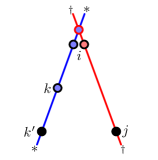
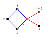
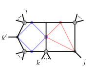
(a)	(b)	(c)

Figure 6: Figure (a) is momentum twistor diagram (with the superfluous edges associated with the external labels dropped), with the endpoints of $\mathcal{L}^{(1)}$ (denoted with $\dagger$) identified, and with the endpoints of $\mathcal{L}^{(2)}$ (denoted with *) identified. The resulting graph (b) comes from preserving the ordering of nodes along the line. Note we have used the ambiguity in ordering between $k$ and $k^{\prime}$ to consider the case $k<k^{\prime}<i$. Mapping any empty node to an edge between massive corners and mapping any filled node to a massless corner with two edges between massive corners, results in the Landau diagram (c). There would be a massive corner along the top of the Landau diagram, but the indices fix that corner to be zero.

In this appendix, we explain how twistor diagrams and Landau diagrams are partial edge-to-node duals of each other. This map straightforwardly generalizes to any number of loops, and is easily inverted to map a Landau diagram into a twistor diagram.

We first note that the edges in a twistor diagram associated with the external labels are redundant, since the “empty” or “filled” property of the node already tracks the same information. So we can drop such edges. Then the following steps map a twistor diagram, $\tau$, to a Landau diagram, $\lambda$:

1. For each loop line $\mathcal{L}^{(i)}$ in $\tau$, identify one endpoint of $\mathcal{L}^{(i)}$ with the other endpoint of $\mathcal{L}^{(i)}$. Since $\tau$ are graphs, this identification preserves the order of the nodes along all $\mathcal{L}^{(i)}$.

2. Map each empty $\tau$-node into a $\lambda$-edge. Identify the two $\lambda$-nodes defining the $\lambda$-edge as massive corners of $\lambda$.

3. Map each filled $\tau$-node into two $\lambda$-edges sharing one common $\lambda$-node. Identify the common $\lambda$-node as a massless corner of $\lambda$, and the other two $\lambda$-nodes as massive corners of $\lambda$.

4. The external labels map from $\tau$ to $\lambda$ such that:

   • the label of an empty $\tau$-node maps to one of the two massless corners defining the new $\lambda$-edge, and

   • the label of a filled $\tau$-node maps into a massless corner of $\lambda$.

This is a partial edge-to-node map because only the empty $\tau$-nodes obey a proper edge-to-node exchange as they map to a $\lambda$-edge, while the filled $\tau$-nodes are effectively unchanged as they map to $\lambda$-nodes. It is always possible to consistently assign the labels of $\tau$ to $\lambda$, though so doing may cause a massive corner of $\lambda$ to completely vanish, as happens in the following concrete example.

We turn now to detailing how the two-loop twistor diagram, Fig. 6(a), (also the first column of Tab. 2(b)) maps into one of its corresponding Landau diagrams, Fig. 6(c) (the second column of Tab. 2(b)).

The first step is to identify the two nodes corresponding to the end-points of each $\mathcal{L}^{(i)}$, $i=1,2$. This closes the two lines into loops, and we formally think of the diagram as a graph, specified by its edges, nodes, and decorations of its nodes. The result is Fig. 6(b), with identified endpoints marked by * and $\dagger$.

In this instance, there is an ambiguity in choosing $k^{\prime}<k$ or $k<k^{\prime}$. We demonstrate the latter case here to highlight that $k^{\prime}$ and $k$ can be swapped with respect to how they appear on the loop line. The $k^{\prime}<k$ differs from what we detail here by swapping ordering of the two nodes along the loop. Then the filled $k^{\prime}$ node would be on the bottom of the box in Fig. 6(b), while the empty $k$ node would be on the left of the box.

In the $k<k^{\prime}$ case we are considering, the resulting graph becomes the Landau diagram, Fig. 6(c) under the partial edge-to-node dual map, as described in the steps above. Note in Fig. 6(c) that the empty nodes of the original twistor diagram are identified with edges of the resulting Landau diagram. In contrast, the filled nodes are identified with massless corners, which are themselves nodes. So this is only a partial edge-to-node map.

References

- (1) T. Dennen, M. Spradlin and A. Volovich, JHEP 1603, 069 (2016) [arXiv:1512.07909 [hep-th]].
- (2) T. Dennen, I. Prlina, M. Spradlin, S. Stanojevic and A. Volovich, JHEP 1706, 152 (2017) [arXiv:1612.02708 [hep-th]].
- (3) I. Prlina, M. Spradlin, J. Stankowicz, S. Stanojevic and A. Volovich, arXiv:1711.11507 [hep-th].
- (4) A. B. Goncharov, M. Spradlin, C. Vergu and A. Volovich, Phys. Rev. Lett. 105, 151605 (2010) [arXiv:1006.5703 [hep-th]].
- (5) J. Maldacena, D. Simmons-Duffin and A. Zhiboedov, JHEP 1701, 013 (2017) [arXiv:1509.03612 [hep-th]].
- (6) L. D. Landau, Nucl. Phys. 13, 181 (1959).
- (7) R. J. Eden, P. V. Landshoff, D. I. Olive and J. C. Polkinghorne, Cambridge University Press, 1966.
- (8) L. J. Dixon, J. M. Drummond and J. M. Henn, JHEP 1111, 023 (2011) [arXiv:1108.4461 [hep-th]].
- (9) L. J. Dixon, J. M. Drummond and J. M. Henn, JHEP 1201, 024 (2012) [arXiv:1111.1704 [hep-th]].
- (10) L. J. Dixon, J. M. Drummond, M. von Hippel and J. Pennington, JHEP 1312, 049 (2013) [arXiv:1308.2276 [hep-th]].
- (11) L. J. Dixon, M. von Hippel and A. J. McLeod, JHEP 1601, 053 (2016) [arXiv:1509.08127 [hep-th]].
- (12) S. Caron-Huot, L. J. Dixon, A. McLeod and M. von Hippel, Phys. Rev. Lett. 117, no. 24, 241601 (2016) [arXiv:1609.00669 [hep-th]].
- (13) J. M. Drummond, G. Papathanasiou and M. Spradlin, JHEP 1503, 072 (2015) [arXiv:1412.3763 [hep-th]].
- (14) L. J. Dixon, J. Drummond, T. Harrington, A. J. McLeod, G. Papathanasiou and M. Spradlin, JHEP 1702, 137 (2017) [arXiv:1612.08976 [hep-th]].
- (15) J. L. Bourjaily, A. J. McLeod, M. Spradlin, M. von Hippel and M. Wilhelm, Phys. Rev. Lett. 120, no. 12, 121603 (2018) [arXiv:1712.02785 [hep-th]].
- (16) D. Nandan, M. F. Paulos, M. Spradlin and A. Volovich, JHEP 1305, 105 (2013) [arXiv:1301.2500 [hep-th]].
- (17) S. Caron-Huot and K. J. Larsen, JHEP 1210, 026 (2012) [arXiv:1205.0801 [hep-ph]].
- (18) N. Arkani-Hamed and J. Trnka, JHEP 1410, 030 (2014) [arXiv:1312.2007 [hep-th]].
- (19) N. Arkani-Hamed, H. Thomas and J. Trnka, JHEP 1801, 016 (2018) [arXiv:1704.05069 [hep-th]].
- (20) N. Arkani-Hamed and J. Trnka, JHEP 1412, 182 (2014) [arXiv:1312.7878 [hep-th]].
- (21) J. M. Drummond, J. Henn, V. A. Smirnov and E. Sokatchev, JHEP 0701, 064 (2007) [hep-th/0607160].
- (22) L. F. Alday and J. M. Maldacena, JHEP 0706, 064 (2007) [arXiv:0705.0303 [hep-th]].
- (23) J. M. Drummond, J. Henn, G. P. Korchemsky and E. Sokatchev, Nucl. Phys. B 828, 317 (2010) [arXiv:0807.1095 [hep-th]].
- (24) N. Arkani-Hamed, J. L. Bourjaily, F. Cachazo, A. B. Goncharov, A. Postnikov and J. Trnka, arXiv:1212.5605 [hep-th].
- (25) N. Arkani-Hamed, J. L. Bourjaily, F. Cachazo and J. Trnka, JHEP 1206, 125 (2012) [arXiv:1012.6032 [hep-th]].
- (26) S. Caron-Huot, JHEP 1112, 066 (2011) [arXiv:1105.5606 [hep-th]].
- (27) S. Caron-Huot and S. He, JHEP 1207, 174 (2012) [arXiv:1112.1060 [hep-th]].
- (28) J. Golden, A. B. Goncharov, M. Spradlin, C. Vergu and A. Volovich, JHEP 1401, 091 (2014) [arXiv:1305.1617 [hep-th]].
- (29) J. Golden and M. Spradlin, JHEP 1502, 002 (2015) [arXiv:1411.3289 [hep-th]].
- (30) J. Drummond, J. Foster and O. Gurdogan, Phys. Rev. Lett. 120, no. 16, 161601 (2018) [arXiv:1710.10953 [hep-th]].
- (31) J. Golden, M. F. Paulos, M. Spradlin and A. Volovich, J. Phys. A 47, no. 47, 474005 (2014) [arXiv:1401.6446 [hep-th]].
- (32) T. Harrington and M. Spradlin, JHEP 1707, 016 (2017) [arXiv:1512.07910 [hep-th]].
- (33) J. Golden and M. Spradlin, JHEP 1309, 111 (2013) [arXiv:1306.1833 [hep-th]].
- (34) N. Arkani-Hamed, J. L. Bourjaily, F. Cachazo and J. Trnka, Phys. Rev. Lett. 113, no. 26, 261603 (2014) [arXiv:1410.0354 [hep-th]].
- (35) Z. Bern, E. Herrmann, S. Litsey, J. Stankowicz and J. Trnka, JHEP 1506, 202 (2015) [arXiv:1412.8584 [hep-th]].
- (36) Z. Bern, E. Herrmann, S. Litsey, J. Stankowicz and J. Trnka, JHEP 1606, 098 (2016) [arXiv:1512.08591 [hep-th]].