Possible Universal Relation Between Short time $\beta$-relaxation and Long time $\alpha$-relaxation in Glass-forming Liquids

Abstract

Relaxation processes in supercooled liquids are known to exhibit interesting as well as complex behavior. One of the hallmarks of this relaxation process observed in the measured auto correlation function is occurrence of multiple steps of relaxation. The shorter time relaxation is known as the $\beta$-relaxation which is believed to be due to the motion of particles in the cage formed by their neighbors. One the other hand longer time relaxation, the $\alpha$-relaxation is believed to be the main relaxation process in the liquids. The timescales of these two relaxations processes dramatically separate out with supercooling. In spite of decades of researches, it is still not clearly known how these relaxation processes are related to each other. In this work we show that, there is a possible universal relation between short time $\beta$-relaxation and the long time $\alpha$-relaxation. This relation is found to be quite robust across many different model systems. Finally we show that length scale obtained from the finite size scaling analysis of $\beta$ timescale is same as that of length scale associated with the dynamic heterogeneity in both two and three dimensions.

Dynamics of supercooled liquids are very complex in nature. The decay of two point density-density auto correlation shows two steps relaxations as the liquid is supercooled. In spite of decades of research the complex dynamical behaviours associated with putative glass transition, is still poorly understood 11BB ; G. Biroli (2012); arcmp ; KDSROPP16 . The density auto correlation function decays to a plateau at shorter time and then at much longer time it finally decays from the plateau to zero in a stretched exponential manner. The short time relaxation in the plateau region is known as $\beta$-relaxation whereas the longer time relaxation is called the $\alpha$-relaxation 11BB ; G. Biroli (2012); JG ; S. Capaccioli (2005); S. Karmakar (2016). Although a lot of efforts have been made to understand the nature of $\alpha$ relaxation and its microscopic origin 11BB ; G. Biroli (2012); arcmp ; KDSROPP16 , far less researches are done to understand the same for shorter time $\beta$-relaxation and its possible connection with the $\alpha$-relaxation steinAdersen ; Karmakar et al. (2015); K. L. Ngai (1998); Hai Bin Yu (1998); K. L. Ngai et al. (1998).

At short times, it is believed that the particles get trapped in transient cage formed by their neighboring particles and they undergo a kind of rattling motion in those cages. Eventually they hop out of the cage and probably after successive such cage breaking processes, the liquid finally relaxes. It is also not clearly known whether the rattling in a cage and subsequent breaking of the cage is the $\beta$-relaxation. If one assumes such an event to be a $\beta$-relaxation and multiple such events leads to $\alpha$-relaxation, then one can expect that short time and long time relaxation processes will be intimately related to each other. Such a scenario is indeed suggested in some studies K. L. Ngai (1998); K. L. Ngai et al. (1998); Karmakar et al. (2015).

In K. L. Ngai (1998), author have proposed a correlation between $\beta$-relaxation time $\tau_{\beta}(T_{g})$ calculated at the experimental glass transition temperature ($T_{g}$), and the Kohlrausch-Williams-Watts (KWW) exponent $(1-n)$ of $\alpha$-relaxation at $T_{g}$. $T_{g}$ is defined experimentally at the temperature where the relaxation time of the liquid becomes $100s$. The KWW exponent is the stretching exponent of the decay profile of the two-point density-density auto correlation function or the self intermediate scattering function as

$$Q(t)=\exp{\left[-\left(\frac{t}{\tau_{\alpha}}\right)^{1-n}\right]},\quad 0\leq n\leq 1,$$ (1)

where $Q(t)=\left<\frac{1}{N}\sum_{i=1}^{N}w(|\vec{r}_{t}(t)-\vec{r}_{i}(0)|)\right>$. The window function $w(x)=1.0$ if $x\leq 0.3$ and $0$ otherwise (see SI for further details). $\langle\ldots\rangle$ represents ensemble average. The $\alpha$ relaxation time is defined as $Q(\tau_{\alpha})=1/e$. At high temperature, the relaxation in liquid is exponential, that is $n=0$, thus one can expect that the nonzero value of $n$ will be related to many body or cooperative nature of the $\alpha$-relaxation process.

The Coupling Model (CM) proposed in K. L. Ngai (1979, 1994); K. Y. Tsang (1997), suggests a relation between primitive relaxation time, $\tau_{0}$ with that of the the $\alpha$-relaxation time as

$$\tau_{\alpha}=\left[\tau_{0}\tau_{c}^{-n}\right]^{1/(1-n)},$$ (2)

where $\tau_{c}$ R. Zorn (1995); J. Colmenero (1993) is the microscopic time scale. $\tau_{0}$, the primitive relaxation time is argued to be close to $\beta$-relaxation time as both of them are assumed to be the precursors of the long time $\alpha$-relaxation process. This relationship has been tested for many glass forming liquids near the experimental glass transition temperature and found to agree with the above relation to varying degree. Fujimori and Ouni’s correlation index $c$ H. Fujimori (1995), defined as $c\equiv 1-\frac{T_{g\beta}}{T_{g\alpha}}$, and the coupling parameter $n$ of CM was also shown subsequently to be linearly proportional to each other for many experimental glass-forming liquids. This clearly suggests that although there are proposals and reports of possible inter-relation between $\tau_{\alpha}$ and $\tau_{\beta}$, a general consensus is still missing.

In a recent study Karmakar et al. (2015), it has been shown that the system size dependence of $\tau_{\beta}$ in three dimensional glass-forming liquids is controlled by the dynamic heterogeneity length ($\xi_{d}$) that are obtained from the finite size scalingS. Karmakar (2009); Privman1990 of peak height of the four-point dynamic susceptibility ($\chi_{4}(t)$, see SI for definition), $\chi_{4}^{P}(T)$arcmp ; S. Karmakar (2009). The peak of $\chi_{4}(t)$ appears at $\alpha$-relaxation time scale, suggesting a very strong inter-relation between these two relaxation processes. Thus a possible universal relation between $\alpha$ and $\beta$ time scale and its origin can be connected to the growth of different length-scales in the system. The main objective of the present work is to revisit this possible relationship between $\tau_{\beta}$ and $\tau_{\alpha}$ and try to explore existence of an universal relationship between these two timescales using more microscopic quantities like dynamic heterogeneity length scale ($\xi_{d}$) and static length scale ($\xi_{s}$) that grow with supercooling arcmp ; KDSROPP16 ; S. Karmakar (2014); G. Biroli (2004).

In this article, we propose a new universal relation between $\beta$-relaxation and $\alpha$-relaxation in model glass-forming liquids and try to rationalize the results within the framework of the well-known Random First Order Transition (RFOT)T. R. Kirkpatrick (1989); V. Lubchenko (2007); G. Biroli (2012) theory of glass transition. Rest of the paper is arranged as follows. First we briefly discuss some of the details of the simulation methods and the models and then we define some relevant correlation functions that are used to calculate different relaxation times and length-scales. A set of new quantities are defined to analyze the data particularly for two dimensional systems. In two dimensions, there will be contribution from long-wave length phonon mode and appropriate corrections need to be made to disentangle the effect due to glass transition and long wavelength density fluctuations on the measured quantities E. Flenner (2015); KABetaPaper ; d1234glass ; weeksPNAS ; KeimPNAS ; gilles2d3d ; Shiba et al. (2016). We then discuss about the relation between $\tau_{\alpha}$ and $\tau_{\beta}$ for both two and three dimensional systems. Effects of finite size on these results are then discussed. Finally we rationalize our observation within the framework of RFOT theory and propose a new universal relationship between $\tau_{\alpha}$ and $\tau_{\beta}$.

We have studied different model systems in two and three dimensions with somewhat different inter particle potentials to make sure that the results obtained are generic and applicable for wide variety of systems. First model is the well known Kob-Andersen binary model where particles interact via Lennard-Jones potential. We refer the model as 3dKAW. Kob (1995). The second model studied is also a binary mixture of particles but with pure repulsive inter particle interactions and this is referred here as 3dR10S. Karmakar (2010). Other models are 3dIPLU. R. Pedersen (2010), 3dHPC. S. O’Hern (2002); S. Chakrabarty (2002), 3dBMLJ_82D. Coslovich (2017). We have done very large system size simulations in three dimensions to remove finite size effects (see SI for further details). We have done simulations for system sizes in the range $N\in{[1000,108000]}$. The data reported in the article is for $N=108000$ only. In two dimensions, we study same Kob-Andersen model and refer it as 2dKA. A slightly modified version of 2dKA model is also studied and will be referred as 2dmKA model. The two dimensional version of 3dR10 model will be referred as 2dR10. A model of polydisperse mixture of particles with truncated Lennard-Jones inter particles interaction potential (also known as WCA potential) in two dimensions is also studied. We refer that model as 2dPoly. The system size in two dimensions ranges from $N\in[100,10000]$. All the details regarding these different models and the simulations details are given in the SI.

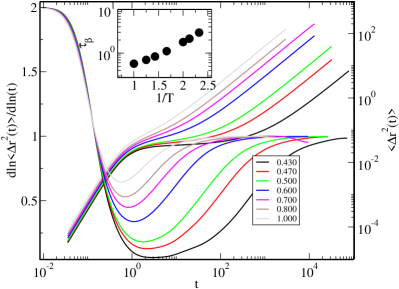
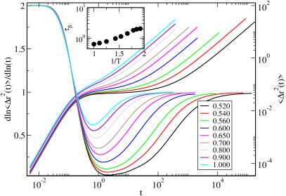
Figure 1: Top panel: Mean square displacement(MSD) and its log-derivative are plotted against time for 3dKA model. In the inset we have shown the temperature dependence of $\tau_{\beta}$ for the same model. The temperature dependence is close to Arrhenius in agreement with previous experimental results. Bottom panel: Similar plot for 3dR10 model. In the inset we show the temperature dependence of $\tau_{\beta}$ for 3dR10 model. For this model also the temperature dependence of $\tau_{\beta}$ follows Arrhenius behavior.

Calculation of $\beta$ time scale: We follow the method given in steinAdersen ; Karmakar et al. (2015) to calculate $\beta$-relaxation timescale, $\tau_{\beta}$ from the mean squared displacement (MSD) which is defined below as

$$\langle|\Delta r(t)|^{2}\rangle=\left\langle\frac{1}{N}\sum_{i=1}^{N}|\vec{r}_{i}(t)-\vec{r}_{i}(0)|^{2}\right\rangle.$$ (3)

MSD shows a point of inflection at an intermediate time, thus if we plot the log-derivative of MSD with time, $d\log{\langle|\Delta r(t)|^{2}\rangle}/d\log{t}$, it will show a dip at that inflection point. $\tau_{\beta}$ is defined as the time where the point of inflection appears. This procedure is shown for 3dKA (top panel) and 3dR10 (bottom panel) models in Fig.1. One can clearly see the minimum in $d\log{\langle|\Delta r(t)|^{2}\rangle}/d\log{t}$ vs $t$ plots and also the minimum shifts to higher and higher values of $t$ with decreasing temperature.

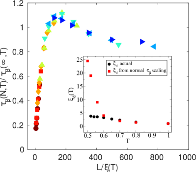
Figure 2: Data collapse of finite size dependence of $\tau_{\beta}$ for 2dR10 mode. Here $\tau_{\beta}$ is obtained from normal MSD (see text for details). Inset shows the variation of length scale with temperature. The scale obtained here are very different than the dynamic heterogeneity length scale of this model system.

In Karmakar et al. (2015), it was shown that the system size dependence of $\tau_{\beta}$ is controlled by the dynamic heterogeneity length scale in three dimensions. To check the validity of the same results in two dimensional models, we have done the finite size scaling (FSS) analysis of $\tau_{\beta}$ for 2dR10 model. The results are shown in Fig.2. $\tau_{\beta}$ has fairly large system size dependence (shown in SI) and the dependence becomes very strong at lower temperatures. Although the data collapse observed is quite good, the obtained length scales as shown in the inset, is found to be very different from the dynamic heterogeneity length scale of this model obtained via different methods.

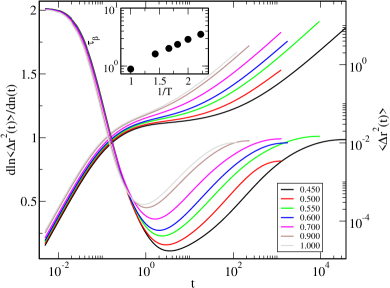
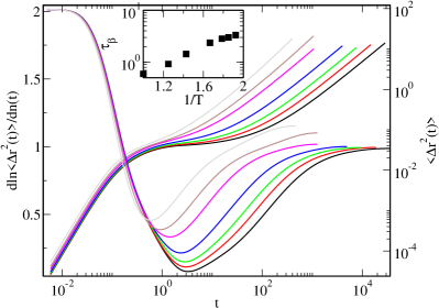
Figure 3: Top panel: Cage-relative mean square displacement(crMSD) and its log-derivative is plotted against time for 2dMKA system. Inset shows the Arrhenius temperature dependence of $\tau_{\beta}$. Bottom panel: Similar plot for the 2dR10 model. Similar Arrhenius temperature dependence of $\tau_{\beta}$ is shown for this model in the inset.

The variation of the length scale in the studied temperature range is very large suggesting a possible contribution coming from long wavelength density fluctuations which are prevalent in two dimensional systems due to Marmin-Wagner theoremND. (2016); ND. Mermin (1968); B. Illing (2017); KeimPNAS . Thus disentangling contributions coming from these long wavelength fluctuations and the glass transition is very important to understand glass transition in two dimensions Shiba et al. (2016); S. Mazoyer (2009); B. Illing (2017). To overcome such a problem in two dimensional system we have calculated cage-relative MSD (crMSD) following Shiba et al. (2016); S. Mazoyer (2009); B. Illing (2017). The crMSD is defined as follows. First we define the cage related displacement of particle $i$ as

$${\Delta}r_{i,CR}(t)={\Delta}r_{i}(t)-\frac{1}{N_{nn}}{\sum_{j\in n.n}{\Delta}r_{j}(t)},$$ (4)

where $N_{nn}$ are the number of nearest neighbor of $i^{th}$ particle, and ${\Delta}r_{j}(t)=r_{j}(t)-r_{j}(0).$ Particles are defined as the neighbors of $i^{th}$ particle if they satisfy $r_{ij}(t)=|r_{j}(t)-r_{j}(0)|<A\sigma_{\alpha\beta}$. $A$ is the cutoff used to define the neighbors. It is usually taken as the distance where first minimum of the radial distribution function $g(r)$ appears. The crMSD is then defined as,

$$\left\langle|{\Delta}r_{CR}(t)|^{2}\right\rangle=\left\langle\frac{1}{N}\sum_{i=1}^{N}|{\Delta}r_{i,CR}(t)|^{2}\right\rangle$$ (5)

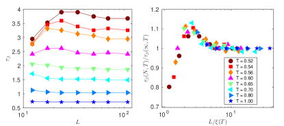
Figure 4: Left panel: System size dependence of $\tau_{\beta}$ obtained from the log-derivative of cage-relative mean square displacement(crMSD) with dynamic heterogeneity length scale as the cutoff (see text for details) for the 2dR10 model. Right panel: Data collapse to obtain the length scale which is found to be same as the dynamic heterogeneity length scale.

As we are measuring relative displacements, it will not be affected by the long wavelength phonon modes and thus one should be able to extract the relevant information from MSD related only to glass transition in two dimensions.

It turns out that the results very much depend on how the neighboring particles are chosen, for example, if one chooses a cutoff at the second minimum in $g(r)$, then one finds a week system size dependence of $\tau_{\beta}$ compare to almost no system size dependence if first minimum of $g(r)$ is chosen. This is somewhat puzzling and seems to constraint the usefulness of the crMSD. One can rationalize these results from the understanding that if one defines a cage relative motion using particles which are its immediate neighbors then one is basically removing even local cooperative motions in the systems. This local cooperative motion has nothing to do with the long wavelength phonon mode.

To keep the cooperative motions undisturbed over the dynamic heterogeneity length scale, we choose the cutoff length for defining the neighbors to be same as the dynamic heterogeneity length. This procedure gives us an estimate of $\tau_{\beta}$ which is not affected by the long wavelength density fluctuations at the same time any possible contributions coming from cooperative motions will not be washed away. In our subsequent analysis we have followed this method to calculate $\tau_{\beta}$. In the top panels of Fig.3, we have shown $d\log{\langle|\Delta r_{CR}(t)|^{2}\rangle}/d\log{t}$ vs $t$ plots for 2dmKA and 2dR10 models. In the inset we show the Arrhenius temperature dependence of $\tau_{\beta}$ for these model systems.

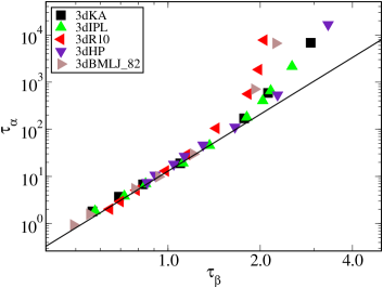
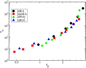
Figure 5: Log-log plot of $\tau_{\alpha}$ vs $\tau_{\beta}$ for all the models systems in three dimensions (top panel) and two dimensions (bottom panel). Power law relation seems not to be valid for all the temperature and data for different models deviate from the master curve at lower temperature in 3d dimensional models. Some quasi-universal relation is observed in two dimensions.

In the left panel of Fig.4, we show the system size dependence of $\tau_{\beta}$ for 2dR10 model and in the right panel we show the finite size scaling of the same data using dynamic heterogeneity length scale, $\xi_{d}$ taken from Ref.I. Tah (2017). The data collapse is indeed reasonable. Thus it can be concluded that finite size scaling of $\tau_{\beta}$ is governed by the dynamic heterogeneity length scale in two dimensions also. This is very similar to the observation reported for three dimensional model Karmakar et al. (2015). This suggests that glass transitions in two and three dimensions share features which are very similar to each other if the effect of long wavelength phonon mode in two dimensions can be disentangled from the measured quantities. Similar observations were made in recent works weeksPNAS ; KeimPNAS ; gilles2d3d ; Shiba et al. (2016); S. Capaccioli (2005); B. Illing (2017).

After calculating $\tau_{\beta}$ and $\tau_{\alpha}$ for all the models in two and three dimensions reliably, we would like to focus our attention on the possible universal relation between these two timescales. As discussed earlier, in Ref.K. L. Ngai (1998), a power law relationship has been proposed between $\tau_{\alpha}$ and $\tau_{\beta}$ as $\tau_{\alpha}\sim\tau_{\beta}^{1/(1-n)}$. As KWW stretching exponent $1-n$ decreases from $1$ with supercooling in a manner which is similar for different model systems, one expects to be able to obtain a master curve by plotting $\tau_{\alpha}$ as a function of $\tau_{\beta}$ for all the temperatures with appropriate choice of the pre-factor in the power law relation. In Fig.5, we have tested the same proposal by plotting $\tau_{\alpha}$ as a function of $\tau_{\beta}$ in log-log plot for both two and three dimensional models.

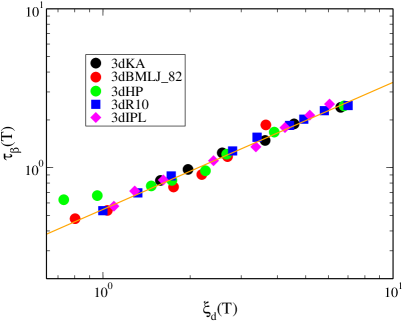
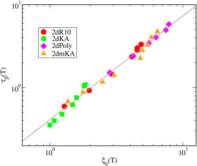
Figure 6: Dynamic scaling relation between $\tau_{\beta}$ and $\xi_{d}$, $\tau_{\beta}\sim\xi_{d}^{z}$. Top panel shows data for all three dimensional model systems with $z\simeq 0.8$ and bottom panel shows data for two dimensional models with $z\simeq 1.25$.

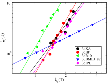
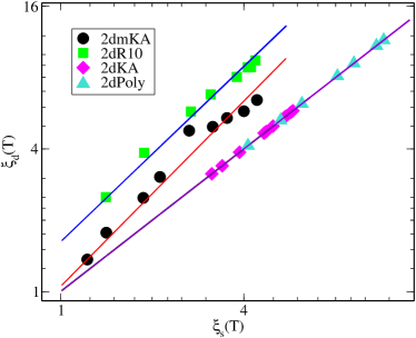
Figure 7: Top panel: Relation between $\xi_{d}$ vs $\xi_{s}$, as $\xi_{d}\sim\xi_{s}^{X}$, with $X=2.7$(3dKA), $3.5$(3dHP), $3.5$(3dR10), $2.8$(3dIPL), $1.0$(BMLJ82) for different three dimensional models. Bottom panel: similar analysis for different two dimensional models with $X=1.30$(2dmKA), $1.23$(2dR10), $1.00$ (2dKA and 2dPoly).

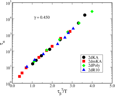
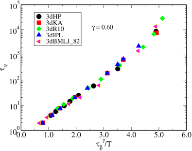
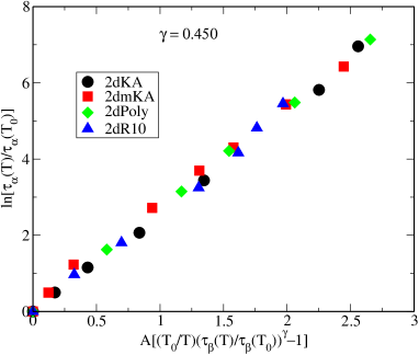
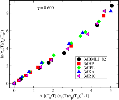
Figure 8: Top left panel: $\tau_{\alpha}$ is plotted against $\tau_{\beta}^{\gamma}/T$ for all the studied two dimensional model systems. Top right panel : Similar plot for all the studied three dimensional model systems. Both in two and three dimensions data follow a master curve which suggests the observed dependence to be very robust. Bottom left panel: $\ln[\frac{\tau_{\alpha}(T)}{\tau_{\alpha}(T_{0})}]$ is plotted against $A[(\frac{T_{0}}{T})(\frac{\tau_{\beta}(T)}{\tau_{\beta}(T_{0})})^{\gamma}-1]$ for all the two dimensional model systems. All the data are clearly on a single master curve with $\gamma=0.45$. Bottom right panel: Similar plot for all the model three dimensional model systems with $\gamma=0.60$.

One can see that the power law relation is not very robust in the studied temperature range for three dimensional systems and deviates strongly especially at lower temperatures. In two dimensions also one sees similar results but data seem to fall on a quasi universal master curve. The observed data collapse although is not very satisfactory. In this work, we propose a simple but robust relation between $\alpha$-relaxation and $\beta$-relaxation time. The form of the proposed relationship between these two timescales can be rationalized within the framework of Random First Order Transition (RFOT) theory T. R. Kirkpatrick (1989); V. Lubchenko (2007); G. Biroli (2012). In RFOT long time structural relaxation time $\tau_{\alpha}$ is connected to static length scale, $\xi_{s}$ via,

$$\tau_{\alpha}(T)=\tau_{\infty}\exp{\left(\frac{{\mu}\xi_{s}^{\psi}}{K_{B}T}\right)}.$$ (6)

As shown in Karmakar et al. (2015) and in present work, finite size effects of $\tau_{\beta}$ can be understood using the dynamic heterogeneity length scale, $\xi_{d}$ in both dimensions, we expect from dynamic scaling arguments that $\tau_{\beta}$ will be related to $\xi_{d}$ as

$$\tau_{\beta}\sim\xi_{d}^{z},$$ (7)

where exponent $z$ is found to be close to $0.8$ for all three dimensional model systems and $z\simeq 1.25$ for all the studied models in two dimensions as shown in Fig.6.

If one assumes that static and dynamic length scales are related as $\xi_{d}\sim\xi_{s}^{X}$, then the following relation between $\tau_{\alpha}$ and $\tau_{\beta}$ can be obtained.

$$\tau_{\alpha}=\tau_{0}\exp{\left(\frac{\Omega\tau_{\beta}^{\gamma}}{K_{B}T}\right)},$$ (8)

where exponent $\gamma=\psi/zX$. Thus if $\tau_{\alpha}$ is plotted as a function of $\tau_{\beta}^{\gamma}/T$, then one would expect to have a master curve if exponent $\gamma$ is universal for all model systems. In general, there is no reasons to expect $\gamma$ to be universal as exponent $\psi$ and $X$ are somewhat different amongst different model systems (see SI for the values of $\psi$ for different models). As shown in Fig.7, exponent $X$ is indeed different for different models in both two and three dimensions. The exponent $X=2.7$, $3.5$, $3.5$, $2.8$ and $1.0$ for 3dKA, 3dHP, 3dR10, 3dIPL and 3dBMLJ_82 respectively. As the range of power law is somewhat restricted, reliable estimate of $X$ is not easy. The values of $X$ for different two dimensional models are $X=1.30$(2dmKA), $1.23$(2dR10), $1.00$ (2dKA and 2dPoly). Note that, there are model systems which show presence of prominent medium range crystalline order at lower temperature or higher density and for them it has been shown that static and dynamic length scales are same I. Tah (2017). 3dBMLJ_82 in three dimensions and 2dKA, 2dPoly in two dimensions are examples of such models. The data for $\xi_{d}$ and $\xi_{s}$ are taken from S. Chakrabarty (2016); I. Tah (2017).

We then test the universality of Eq.8, for different two and three dimensional model systems. In top panels of Fig.8, we have plotted $\tau_{\alpha}$ as a function of $\tau_{\beta}^{\gamma}/T$ with $\gamma=0.60$ for three dimensions (top left panel) and $\gamma=0.45$ for two dimensions (top right panel). In these plots we have adjusted the values of non-universal parameters like $\tau_{0}$ and $\Omega$ in Eq.8 to collapse all the data on a master curve. The quality of collapse clearly suggest that indeed $\tau_{\alpha}$ is universally related to $\tau_{\beta}$ via Eq.8 with a universal exponent $\gamma$.

Now one might suspect the reliability of the above relation as $\tau_{0}$ and $\Omega$ are varied freely, to eliminate dependence on $\tau_{0}$, we take a reference temperature $T_{0}$ (highest temperature studied for each model) and divide Eq.8 from both sides to write,

$$\log\left[\frac{\tau_{\alpha}(T)}{\tau_{\alpha}(T_{0})}\right]=\Omega\left[\left(\frac{T_{0}}{T}\right)\left(\frac{\tau_{\beta}(T)}{\tau_{\beta}(T_{0})}\right)^{\gamma}-1\right]$$ (9)

Eq.9, keeps only one parameter free and that is $\Omega$. In bottom panels of Fig.8, we have plotted $\log\left[\frac{\tau_{\alpha}(T)}{\tau_{\alpha}(T_{0})}\right]$ vs $\frac{T_{0}}{T}\left(\frac{\tau_{\beta}(T)}{\tau_{\beta}(T_{0})}\right)^{\gamma}-1$ for both two and three dimensions. The observed data collapse again reconfirms the proposed universal relation between $\tau_{\alpha}$ and $\tau_{\beta}$. Using reported values of $\psi$ for the different models (see SI for the details), one obtains the values of $\gamma$ to be close to $0.51,0.79,0.66$ and $0.54$ for 3dKA, 3dHP, 3dR10 and 3dIPL models. These numbers are in agreement with the chosen value of $\gamma=0.6$ for three dimensional models. However, the exponent turns out to be somewhat different for 3dBMLJ_82 model ($\gamma\simeq 1.125$). We believe that this discrepancy is probably due to uncertainties in the values of $\psi,z$ as well as $X$. For two dimensional models, the numbers are $0.43,0.58,0.57$ and $0.54$ for 2dmKA, 2dR10, 2dPoly, and 2dKA respectively. Thus the numbers are in agreement with the universal number $\gamma=0.45$ for two dimensions.

If the proposed universal relation between $\tau_{\alpha}$ and $\tau_{\beta}$ is shown to be valid for experimentally relevant glass forming liquids, then one might be able to understand the vitrification in liquids by probably understanding the $\beta$-relaxation processes only. This might lead us to identify the relevant elementary relaxation process responsible for both $\beta$ and $\alpha$ relaxation in glassy systems. On a slightly different note, it was shown in M. Mukherjee (2017) that the collapsing dynamics of a polymer chain in a supercooled liquid is controlled by both $\alpha$ and $\beta$ relaxation processes with possible implications in bio-preservation. It is suggested that not only $\alpha$-relaxation but also $\beta$-relaxation should be taken into account in order to understand the degradation process of biomolecules CiceroneDouglasBioPhyJ2004 ; CiceroneDouglasSoftMatter2012 . Thus our proposed universal relation between these two relaxation processes might help us design the appropriate glassy matrix in future to preserve bio-macromolecules more efficiently.

To conclude, we have shown that there is a universal relation between $\alpha$ and $\beta$ relaxation times of glass forming liquids. The proposed relation is different from the one predicted by Coupling Model K. L. Ngai (1998). The new relation can be rationalized within the framework of Random First Order Transition Theory. In two dimensions, due to long wavelength density fluctuations, different transport quantities show logarithmic system size dependence and disentangling this effect from the effect emanating from glass transition is often difficult. We show how $\tau_{\beta}$ can be calculated in two dimensions by appropriately modifying the correlation functions to remove the effect of long wavelength phonon without affecting the cooperative motions at the relevant dynamical heterogeneity length scale. We then shown that finite size scaling of $\tau_{\beta}$ is controlled by the dynamic heterogeneity length scale as in the three dimensional models. Finally, the obtained universal relationship between $\tau_{\alpha}$ and $\tau_{\beta}$ in both the dimensions suggests that the physics of glass transition may be very similar in both two and three dimensions. This observation is in agreement with recent findings weeksPNAS ; KeimPNAS ; gilles2d3d . As $\beta$-relaxation plays in important role below the glass transition, in future it will be very interesting and important for industrial applications to study possible aging behavior of $\tau_{\beta}$ and its correlation with the aging behavior of $\tau_{\alpha}$.

- (1) L. Berthier and G. Biroli, Rev. Mod. Phys. 83,587–645, (2011).
- G. Biroli (2012) G. Biroli and J.-P. Bouchaud Structural Glasses and Supercooled Liquids: Theory, Experiment, and Applications 31–113 (2012)
- (3) S. Karmakar, C. Dasgupta, and S. Sastry, Annu. Rev. Condens. Matter Phys. 5, 255 (2014).
- (4) S. Karmakar, C. Dasgupta and S. Sastry, Rep. Prog. Phys., 79, 2016.
- (5) G. P. Johari and M. Goldstein, J. Chem. Phys. 53 2372 (1970).
- S. Capaccioli (2005) S. Capaccioli, and K.L Ngai, J. Phys. Chem. B 109, 9727-9735 (2005)
- S. Karmakar (2016) S. Karmakar, Journal of Physics: Conference Series 759 012008 (2016)
- (8) R.S.L. Stein and H.C. Andersen, Phys. Rev. Lett. 101, 267802 (2008).
- Karmakar et al. (2015) S. Karmakar, C. Dasgupta, S. Sastry Phys. Rev. Lett. p. 116, 085701 (2016)
- K. L. Ngai (1998) K.L. Ngai, The Journal of Chemical Physics p. 109, 6982 (1998)
- Hai Bin Yu (1998) H.B. Yu, W.H. Wang, H.Y. Bai, and K. Samwer National Science Review, Vol. 1, No. 3 (2014)
- K. L. Ngai et al. (1998) K.L. Ngai, Z: Wang, X.Q. Gao H.B. Yu,and W.H. Wang The Journal of Chemical Physics p. 139, 014502 (2013)
- K. L. Ngai (1979) K. L. Ngai, Solid State Phys. 9, 121 (1979)
- K. L. Ngai (1994) K. L. Ngai, in Disorder Effects on Relaxational Properties, edited by R. Richert and A. Blumen͑Springer, Berlin, 89–150. (1994)
- K. Y. Tsang (1997) K. Y. Tsang , and K. L. Ngai , Phys. Rev. E 54.R3067 1996; 56, R17 (1997)
- R. Zorn (1995) R. Zorn, A. Arbe, J. Colmenero, B. Frick, D. Richter and U. Buchenau, Phys. Rev. E, 52, 781 (1995)
- J. Colmenero (1993) J. Colmenero, A. Arbe and A. Alegria, Phys. Rev. Lett. 71, 2603 (1993)
- H. Fujimori (1995) H. Fujimori , and M. Oguni , Solid State Commun. 94, 157 (1995)
- S. Karmakar (2009) S. Karmakar, C. Dasgupta and S. Sastry Proc. Natl. Acad.Sci. U.S.A. 106, 3675 (2009)
- (20) Finite Size Scaling and Numerical Simulations in Statistical Systems, World Scientific, Singapore, edited by V. Privman (1990)
- S. Karmakar (2014) S. Karmakar, C. Dasgupta and S. Sastry Annu. Rev. Condens. Matter Phys. 5, 255 (2014)
- G. Biroli (2004) G. Biroli, J.-P. Bouchaud K. Miyazaki and D. R. Reichman, Phys. Rev. Lett. 97, 195701 (2006)
- T. R. Kirkpatrick (1989) T. R. Kirkpatrick, D. Thirumalai and P. G. Wolynes Phys.Rev.A. 40, 1045 (1989)
- V. Lubchenko (2007) V. Lubchenko and P. G. Wolynes Annu. Rev. Phys. Chem. 58, 235 (2007)
- E. Flenner (2015) E. Flenner,and G. Szamel, Nat Commun 6:7392 (2015)
- (26) W. Kob and H.C. Andersen, Phys. Rev. Lett. 73, 1376 (1994).
- (27) R. Brüning, DA. St-Onge, S. Patterson, and W. Kob, J. Phys. Condens. Matter 21, 035117 (2009).
- (28) S. Vivek, C.P. Kelleher, P.M. Chaikin, and E.R. Weeks, Proc. Natl. Acad. Sci. (USA), 114 1850 (2017).
- (29) B. Illing, S. Fritschi, H. Kaiser, C.L. Klix, G. Maret, and P. Keim, Proc Natl Acad Sci USA 114 1856 (2017).
- (30) G. Tarjus, Proc Natl Acad Sci USA 114, 2440 (2017).
- Shiba et al. (2016) H. Shiba, Y. Yamada, T. Kawasaki, and K. Kim, Phys. Rev. Lett. p. 117.245701 (2016)
- W. Kob (1995) W. Kob and H. C. Andersen, Phys. Rev. E 51 4626 (1995)
- S. Karmakar (2010) S. Karmakar, E. Lerner, I. Procaccia and J. Zylberg, Phys. Rev. E, 82 031301 (2010)
- U. R. Pedersen (2010) U. R. Pedersen, T. B. Schroder and J. C. Dyre, Phys. Rev. Lett, 105 157801 (2010)
- C. S. O’Hern (2002) C. S. O’Hern, S. A. Langer, A. J. Liu and S. R. Nagel, Phys. Rev. Lett, 88 075507 (2002)
- S. Chakrabarty (2002) S. Chakrabarty, I. Tah, S. Karmakar and C. Dasgupta, Phys. Rev. Lett, 119 205502 (2017).
- D. Coslovich (2017) D. Coslovich and G. Pastore The Journal of Chemical Physics 127, 124504 (2007).
- ND. (2016) ND. Mermin,and H. Wagner, Phys Rev Lett 17:1133–1136 (1966)
- ND. Mermin (1968) ND. Mermin, Phys Rev 176:250–254 (1968)
- B. Illing (2017) B. Illing, S. Fritschia, H. Kaiser Christian L. Klix, G. Maret P. Keim, PNAS 1856–1861,vol. 114,no. 8 (2017)
- S. Mazoyer (2009) S. Mazoyer, F. Ebert, G. Maret and P. Keim, EPL 88 66004 (2009)
- I. Tah (2017) I. Tah, S. Sengupta, S. Sastry, C. Dasgupta, and S. Karmakar, arXiv: 1705.09532 (2017)
- S. Chakrabarty (2016) S. Chakrabarty, R. Das,and S. Karmakar, The Journal of Chemical Physics 145, 034507 (2017)
- M. Mukherjee (2017) M. Mukherjee, J. Mondal and S. Karmakar, arXiv: 1709.09475 (2017)
- (45) M.T. Cicerone and J.F. Douglas, -relaxation governs protein stability in sugar-glass matrices. Soft Matter, 8, 2983, (2012).
- (46) M.T. Cicerone and C.L. Soles, Fast dynamics and stabilization of proteins: Binary glasses of trehalose and glycerol, Biophysical Journal, 86, 3836–3845, (2004).