A perturbative approach to control variates in molecular dynamics

Abstract

We propose a general variance reduction strategy to compute averages with diffusion processes. Our approach does not require the knowledge of the measure which is sampled, which may indeed be unknown as for nonequilibrium dynamics in statistical physics. We show by a perturbative argument that a control variate computed for a simplified version of the model can provide an efficient control variate for the actual problem at hand. We illustrate our method with numerical experiments and show how the control variate is built in three practical cases: the computation of the mobility of a particle in a periodic potential; the thermal flux in atom chains, relying on a harmonic approximation; and the mean length of a dimer in a solvent under shear, using a non-solvated dimer as the approximation.

1 Introduction

Diffusion processes have won an increasing interest in the past years in the statistical physics community, to model physical phenomena and to sample the underlying probability measure characterizing the state of the system [6]. The average value of a thermodynamic function $R$ (as the energy, the pressure, a length, a flux, …) under this probability distribution is given by an integral over the very high-dimensional configurational space. An important motivation for this work is the averaging of mean properties for systems subject to an external driving. In this case the invariant probability measure is often not known explicitly. The goal can be to compute a transport coefficient, a free energy or more generally the response to a non-equilibrium forcing. From a practical point of view, the unknown probability measure is sampled by integrating a stochastic dynamics [1, 22, 67, 40]

$$\differential X_{t}=b(X_{t})\,\differential t+\sigma(X_{t})\,\differential W_{t}.$$ (1)

Two prototypical dynamics in molecular simulation are the Langevin and overdamped Langevin dynamics [1, 39]. At equilibrium, the Langevin dynamics evolves positions $q$ and momenta $p$ as

$$\left\{\begin{aligned} \differential q_{t}&=\frac{p_{t}}{m}\,\differential t,\\ \differential p_{t}&=-\nabla V(q_{t})\,\differential t-\frac{\gamma}{m}p_{t}\,\differential t+\sqrt{2\gamma\beta^{-1}}\,\differential W_{t},\end{aligned}\right.$$ (2)

where $\gamma>0$ is the friction coefficient, $m>0$ is the mass of a particle and $\beta>0$ is proportional to the inverse temperature. The potential energy function is denoted by $V$ and $W_{t}$ is a multi-dimensional standard Brownian motion. In the limit of large frictions $\gamma$, this equation becomes after proper rescaling the overdamped Langevin dynamics [21]:

$$\differential q_{t}=-\nabla V(q_{t})\,\differential t+\sqrt{2\beta^{-1}}\,\differential W_{t}.$$ (3)

Nonequilibrium versions of the above dynamics are obtained for instance by considering non-gradient forces rather than $-\nabla V$.

For any ergodic dynamics (1), macroscopic properties are computed via averages over a trajectory as

$$\mathbb{E}[R]:=\lim_{T\to\infty}\widehat{R}_{T}\quad\mbox{a.s.},\qquad\widehat{R}_{T}=\frac{1}{T}\int_{0}^{T}R(X_{t})\,\differential t.$$

The statistical error for these estimators is characterized by the asymptotic variance:

$$\sigma_{R}^{2}=\lim_{T\to\infty}T\,\mathrm{Var}\left[\widehat{R}_{T}\right].$$ (4)

In many cases of interest ergodic means converge very slowly, requiring the use of variance reduction techniques to speed up the computation. Two types of phenomena can lead to large statistical errors: first, the metastability arising from multimodal potentials, which can greatly increase the correlation of the trajectory in time and lead to large variances; second, a high signal-to-noise ratio, which is typical when averaging small linear responses as for the computation of transport coefficients [18, 67].

When the system is at equilibrium, by which we mean that detailed balance holds, the invariant probability measure is often known and it is possible to use standard variance reduction techniques [58, 20, 10, 45, 38] such as importance sampling [13, 45] or stratification [23, 47, 34, 63, 60]. This allows to address both metastability issues and high noise-to-signal ratios.

For non-equilibrium systems, and more generally when the invariant probability measure is not known, reducing the variance is challenging since standard variance reduction methods cannot be used. Note that reducing the metastability would require modifying the dynamics while keeping the invariant probability measure unchanged, or at least knowing how it changes (see for instance [42, Section 3.4]). When the latter is not known, this task is hard to perform. On the other hand increasing the signal-to-noise ratio is feasible even for non-equilibrium dynamics. This is the goal of the present work, where we rely on control variates. Control variates laying on the concept of "zero-variance" principle have been already used in molecular simulation [3]. This approach was also studied in Bayesian inference simulations [28, 48, 14, 49, 51], where configurations are sampled with Markov chains rather than diffusion processes. This type of techniques has however been restricted to cases where the invariant probability measure is known, except for specific settings such as [24], where a coupling strategy is described.

In the present work, which relies on ideas announced in [42, Section 3.4.2], control variates are constructed without any knowledge of the expression of the invariant probability measure. We build an unbiased modified observable $R+\xi=R+\mathcal{L}\Phi$, where $\mathcal{L}$ is the generator of the dynamics, which is of smaller variance (at least in some asymptotic regime):

$$\mathbb{E}[R+\xi]=\mathbb{E}[R]\quad\mbox{and}\quad\sigma_{R+\xi}^{2}<\sigma_{R}^{2}.$$

The optimal choice for the control variate $\xi$ is $\xi=\mathcal{L}\Phi$ where $\Phi$ is the solution of the following Poisson equation:

$$-\mathcal{L}\Phi=R-\mathbb{E}[R].$$

The general strategy we consider consists in approximating this partial differential equation (PDE) by a simplified one, with an operator $\mathcal{L}_{0}$, for which the solution ${\Phi_{0}}$ can be analytically computed or numerically approximated with a good precision. Theorems 2 and 4 provide an analysis of the asymptotic variance $\sigma_{R+\xi}^{2}$.

We present numerical results illustrating the general method in three practical cases. In particular we provide in each case a simplified process, associated to a simplified Poisson problem. In these applications we are interested in averaging the linear response of an observable with respect to a non-equilibrium perturbation. This is a challenging class of problems since the average quantity is small and thus the relative statistical error is large. We present the problems we consider by increasing complexity of the setup. We start with the computation of the mobility of a particle in a periodic two-dimensional potential. The control variate can be approached with a very high precision by a numerical method based on a spectral basis, allowing to illustrate Theorem 4. We next estimate the conductivity of an atom chain [8, 44, 15]. The number of state variables is much larger (up to several hundreds of degrees of freedom in our simulations) but the geometrical setting is one-dimensional. The control variate can be computed analytically when taking a harmonic model as a reference, and thus it does not require any additional numerical procedure. The third application is a dimer in a solvent, whose mean length is estimated under an external shearing force. In the latter case the difficulty comes from the fact that the system is high-dimensional and not as structured as the atom chain.

This article is organized as follows. We present in Section 2 the general strategy for building control variates and state a result making precise how control variates behave in a perturbative framework. We then turn to the case of a single particle in a one-dimensional periodic potential under a non-gradient forcing in Section 3; the computation of the thermal flux passing through a chain in Section 4; and the estimation of the mean length of a dimer in a solvent under an external shearing stress in Section 5. Some technical results are gathered in the appendices.

2 General strategy

The definition of the asymptotic variance of time averages along a trajectory requires to introduce more precisely the generator of the process and some associated functional spaces, which is done in Section 2.1. The concept of control variate is then explained Section 2.2, as well as the so-called "zero-variance principle". We give in Section 2.3 our perturbative construction of control variate in an abstract setting and state the main theorem quantifying the variance reduction in a limiting regime. Finally Section 2.4 provides a generalized version of this theorem in the case when an approximate solver is used.

2.1 Asymptotic variance

The state space $\mathcal{X}$ is typically the full space $\mathbb{R}^{d}$ or a bounded domain with periodic boundary conditions $\mathbb{T}^{d}$. For some dynamics such as Langevin dynamics, auxiliary variables with values in $\mathbb{R}^{d}$ are added, so that in this case $\mathcal{X}=\mathbb{R}^{d}\times\mathbb{R}^{d}$ or $\mathcal{X}=\mathbb{T}^{d}\times\mathbb{R}^{d}$. As suggested in the introduction, we decompose the generator of the process (1) as a sum $\mathcal{L}=\mathcal{L}_{0}+\widetilde{\mathcal{L}}$ of a reference generator $\mathcal{L}_{0}$ and a perturbation $\widetilde{\mathcal{L}}$. In order to study the asymptotic regime corresponding to small perturbations, we use a parameter $\eta\in\mathbb{R}$ to interpolate smoothly between $\mathcal{L}_{0}$ and $\mathcal{L}$, and define

$$\mathcal{L}_{\eta}=\mathcal{L}_{0}+\eta\widetilde{\mathcal{L}}.$$

We suppose that these operators $\mathcal{L}_{\eta}$ write:

$$\mathcal{L}_{\eta}=b_{\eta}\cdot\nabla+\frac{1}{2}\sigma_{\eta}\sigma_{\eta}^{\top}:\nabla^{2}=\sum_{i=1}^{d}\left(b_{\eta}\right)_{i}\partial_{x_{i}}+\frac{1}{2}\sum_{i,j=1}^{d}\left(\sigma_{\eta}\sigma_{\eta}^{\top}\right)_{i,j}\partial_{x_{i}x_{j}},$$

with $b_{\eta}$ and $\sigma_{\eta}$ are smooth. They are then the generators of the following stochastic processes on $\mathcal{X}$, indexed by $\eta$:

$$\differential X_{t}^{\eta}=b_{\eta}(X_{t}^{\eta})\,\differential t+\sigma_{\eta}(X_{t}^{\eta})\,\differential W_{t},$$ (5)

where $W_{t}$ is a $d$-dimensional standard Brownian motion. Let us assume that $b_{\eta}$ and $\sigma_{\eta}$ are such that the following holds.

Assumption 1.

The dynamics (5) admits a unique invariant probability measure $\pi_{\eta}$ for any $\eta\in\mathbb{R}$. Moreover, trajectorial ergodicity holds: for any observable $R\in\mathrm{L}^{1}(\pi_{\eta})$,

$$\mathbb{E}_{\eta}[R]:=\int_{\mathcal{X}}R(x)\,\differential\pi_{\eta}(x)=\lim_{T\to\infty}\frac{1}{T}\int_{0}^{T}R(X_{t}^{\eta})\,\differential t\quad\mathrm{a.s.}$$

Sufficient conditions for this to hold are discussed after Assumption 2. Let us now make the functional spaces precise. We denote by $(\mathcal{K}_{n})_{n\in\mathbb{N}}$ a family of so-called Lyapunov functions with values in $[1,+\infty)$. The associated weighted $\mathrm{L}^{\infty}$ spaces are:

$$\forall n\in\mathbb{N},\quad{\mathrm{L}_{n}^{\infty}} =\left\{\varphi\ \mbox{measurable}\ \left|\ \|\varphi\|_{\mathrm{L}_{n}^{\infty}}<\infty\right.\right\},\qquad\|\varphi\|_{\mathrm{L}_{n}^{\infty}}=\left\|\frac{\varphi}{\mathcal{K}_{n}}\right\|_{\mathrm{L}^{\infty}}.$$

We make the following assumption on the Lyapunov functions.

Assumption 2.

For any $\eta\in\mathbb{R}$, the function $\mathcal{K}_{n}$ belongs to ${\mathrm{L}^{2}(\pi_{\eta})}$. In particular,

$$\forall n\in\mathbb{N},\,\forall\eta\in\mathbb{R},\quad{\mathrm{L}_{n}^{\infty}}\subset{\mathrm{L}^{2}(\pi_{\eta})}.$$

We also assume that for any $n,n^{\prime}\in\mathbb{N}$, there exists $m\in\mathbb{N}$ such that $\mathcal{K}_{n}\mathcal{K}_{n^{\prime}}\in{\mathrm{L}_{m}^{\infty}}$.

The first part of Assumption 2 is typically obtained by using a family of Lyapunov functions satisfying conditions of the form

$$\mathcal{L}_{\eta}\mathcal{K}_{n}\leqslant-\alpha_{n,\eta}\mathcal{K}_{n}+b_{n,\eta},$$ (6)

for some $\alpha_{n,\eta}>0$ and $b_{n,\eta}\in\mathbb{R}$. Indeed, after integration against $\pi_{\eta}$,

$$0=\int_{\mathcal{X}}\mathcal{L}_{\eta}\mathcal{K}_{n}\differential\pi_{\eta}\leqslant-\alpha_{n,\eta}\int_{\mathcal{X}}\mathcal{K}_{n}\differential\pi_{\eta}+b_{n,\eta},$$

so that

$$1\leqslant\int_{\mathcal{X}}\mathcal{K}_{n}\differential\pi_{\eta}\leqslant\frac{b_{n,\eta}}{\alpha_{n,\eta}}.$$

We can then conclude with the second part of Assumption 2 since, for any $n\geqslant 1$, there exist $C_{n}>0$ and $m\geqslant 1$ such that $1\leqslant\mathcal{K}_{n}^{2}\leqslant C_{n}\mathcal{K}_{m}$. The condition (6) also implies the existence of an invariant probability measure for any $\eta\in\mathbb{R}$ when a minorization condition holds [27]. A typical choice for the Lyapunov functions are the polynomials $\mathcal{K}_{n}(x)=1+|x|^{n}$. This choice satisfies the second part of Assumption 2 when the invariant probability measure has moments of any order. Unless otherwise mentioned, we always consider this choice in the sequel (which is standard for Langevin and overdamped Langevin dynamics, see [62, 46, 35, 36]). As for Assumption 1, trajectorial ergodicity holds when the generator $\mathcal{L}_{\eta}$ is elliptic or hypoelliptic, and there exists an invariant probability measure with positive density with respect to the Lebesgue measure [33]. The latter condition follows if the measure which appears in the minorization condition has a positive density with respect to the Lebesgue measure.

We denote for any function $\varphi\in\mathrm{L}^{1}(\pi_{\eta})$ the projection on the space of mean zero functions by:

$$\Pi_{\eta}\varphi=\varphi-\mathbb{E}_{\eta}[\varphi].$$

For any operator $A\in\mathcal{B}(E)$ (bounded on the Banach space $E$), the operator norm is defined as

$$\|A\|_{\mathcal{B}(E)}=\sup_{\|\varphi\|_{E}=1}\|A\varphi\|_{E}.$$

Let us now make the following assumption.

Assumption 3.

For any $n\in\mathbb{N}$, the $\mathrm{L}^{2}(\pi_{\eta})$ norms of the Lyapunov functions are uniformly bounded on compact sets of $\eta$: for any $\eta_{*}>0$ there exists a constant $C_{n,\eta_{*}}$ such that

$$\forall|\eta|\leqslant\eta_{*},\quad\|\mathcal{K}_{n}\|_{\mathrm{L}^{2}(\pi_{\eta})}\leqslant C_{n,\eta_{*}}.$$ (7)

Moreover $\mathcal{L}_{\eta}$ is invertible on $\Pi_{\eta}{\mathrm{L}_{n}^{\infty}}$. Finally the inverse generator is bounded uniformly on compact sets of $\eta$:

$$\forall|\eta|\leqslant\eta_{*},\quad\left\|-{\mathcal{L}_{\eta}^{-1}}\right\|_{\mathcal{B}\left(\Pi_{\eta}{\mathrm{L}_{n}^{\infty}}\right)}\leqslant C_{n,\eta_{*}}.$$ (8)

The invertibility of $\mathcal{L}_{\eta}$ on $\Pi_{\eta}{\mathrm{L}_{n}^{\infty}}$ is a standard result which follows typically from the Lyapunov conditions (6) and a so-called minorization condition [27]. It has been proved for a large variety of problems [17, 62, 46, 35, 36]. Conditions (7) and (8) are needed to prove Theorems 2 and 4 to come. Condition 7 can be obtained by showing uniform bounds on the coefficients which appear in the Lyapunov conditions, while condition (8) additionally requires some uniformity on the minorization condition.

When Assumptions 1 to 3 hold, the asymptotic variance introduced in (4) is finite for any $\varphi\in{\mathrm{L}_{n}^{\infty}}$ and the following formula holds [42]:

$$\sigma_{\varphi,\eta}^{2}=2\left\langle\varphi,-{\mathcal{L}_{\eta}^{-1}}\Pi_{\eta}\varphi\right\rangle_{\eta},$$ (9)

where $\left\langle\cdot,\cdot\right\rangle_{\eta}$ denotes the canonical scalar product on ${\mathrm{L}^{2}(\pi_{\eta})}$. We refer to Appendix D for more details on the numerical estimation of the asymptotic variance.

Remark 1.

We choose to work directly with weighted $\mathrm{L}^{\infty}$ spaces as this is the relevant setting for Theorems 2 and 4. Note that the asymptotic variance of an observable $\varphi\in{\mathrm{L}^{2}(\pi_{\eta})}$ can also be defined using perturbative arguments relatively to an equilibrium reference dynamics [16, 30]. Contrarily to the ${\mathrm{L}_{n}^{\infty}}$ framework one would however be restricted in this case to small non-equilibrium perturbations.

2.2 Ideal control variate

We recall in this section what a control variate is in our context and show how the construction of an optimal control variate can be reformulated as solving a Poisson problem. The functional framework is made precise in a second step using Assumption 3. We say that a function $\xi$ is a control variate of the observable $R$ for the process $X_{t}^{\eta}$ with generator $\mathcal{L}_{\eta}$ if

$$\mathbb{E}_{\eta}[R+\xi]=\mathbb{E}_{\eta}[R]\quad\mbox{and}\quad\sigma_{R+\xi,\eta}^{2}<\sigma_{R,\eta}^{2}.$$

The principle of our method, already explained in [42], is based on the equation which characterizes the invariance of the measure $\pi_{\eta}$: for any function $\Phi$,

$$\mathbb{E}_{\eta}[\mathcal{L}_{\eta}\Phi]=0.$$

This shows that control variates $\xi$ of the form $\xi=\mathcal{L}_{\eta}\Phi$ automatically ensure that $\mathbb{E}_{\eta}[R+\xi]=\mathbb{E}_{\eta}[R]$, whatever the choice of $\Phi$. In order for $\xi$ to be a good control variate, the modified observable $R+\xi=R+\mathcal{L}_{\eta}\Phi$ should however be of small asymptotic variance. The optimal choice, denoted by $\Phi_{\eta}$ and referred to as the "zero-variance principle" [3, 48], is to make the modified observable constant. This constant is then necessarily equal to $\mathbb{E}_{\eta}[R]$, and $\Phi_{\eta}$ is the solution of the Poisson problem:

$$-\mathcal{L}_{\eta}\Phi_{\eta}=R-\mathbb{E}_{\eta}[R].$$ (10)

Assuming that $R\in{\mathrm{L}_{n}^{\infty}}$ for some $n\in\mathbb{N}$, the problem (10) admits a unique solution $\Phi_{\eta}\in{\mathrm{L}_{n}^{\infty}}$ when Assumption 3 holds.

In practice two problems arise when trying to solve (10). First, the equation (10) is a very high-dimensional PDE for most purposes and the complexity of such problems scales exponentially with the dimension. Second, $\mathbb{E}_{\eta}[R]$ is not known since it is precisely the quantity we are trying to compute. We discuss in the next section how to approximate the solution of (10), at least for small $\eta$.

2.3 Perturbative control variate

The key assumption in our approach is to assume that we can compute the solution $\Phi_{0}$ of the reference Poisson problem corresponding to $\eta=0$:

$$-\mathcal{L}_{0}\Phi_{0}=R-\mathbb{E}_{0}[R].$$ (11)

In practice $\mathcal{L}_{0}$ is the generator of a simplified dynamics (depending on the problem), and $\mathcal{L}_{\eta}$ is the generator of the problem at hand (say for $\eta=1$). Let us emphasize that the dynamics associted with $\mathcal{L}_{0}$ need not be an equilibrium dynamics (see the example discussed in Section 4). The small parameter $\eta$ is used to quantify the discrepancy between the optimal function $\Phi_{\eta}$ and its approximation ${\Phi_{0}}$ in a perturbative framework. We refer to Section 2.4 for a discussion on the numerical resolution of (11), and to the end of this section for further comments on the decomposition.

We define the so-called core space $\mathcal{S}$ as the set of all $\mathcal{C}^{\infty}$ functions which grow at infinity at most like $K_{n}$ for some $n$, and whose derivatives also grow at most like $K_{n}$ for some $n$. Such a space was considered in [62] for instance. More precisely,

$$\mathcal{S} =\big{\{}\varphi\in\mathcal{C}^{\infty}(\mathcal{X})\big{|}\ \forall k\in\mathbb{N},\,\exists n\in\mathbb{N},\quad\partial_{k}\varphi\in{\mathrm{L}_{n}^{\infty}}\big{\}}.$$ (12)

The space $\mathcal{S}$ is dense in ${\mathrm{L}^{2}(\pi_{\eta})}$ under Assumption 2, since $\mathcal{C}^{\infty}$ functions with compact support are included in $\mathcal{S}$. We need an additional assumption in our analysis to ensure that ${\Phi_{0}}\in\mathcal{S}$.

Assumption 4.

The space $\mathcal{S}$ is stable by the generator $\mathcal{L}_{0}$ and $\mathcal{L}_{0}$ is invertible on the space $\Pi_{0}\mathcal{S}$ composed of functions with average $0$ with respect to the invariant probability measure $\pi_{0}$. This means that, for any $\varphi\in\Pi_{0}\mathcal{S}$, there exists a unique solution $\psi\in\Pi_{0}\mathcal{S}$ to the Poisson equation

$$-\mathcal{L}_{0}\psi=\varphi.$$

Assumption 4 can be proved to hold for Langevin and overdamped Langevin dynamics at equilibrium under certain assumptions on the potential $V$, see [62, 35, 36]. The generator of the perturbation should also satisfy the following condition.

Assumption 5.

The generator $\widetilde{\mathcal{L}}$ of the perturbation is such that $\mathcal{S}$ is stable by $\widetilde{\mathcal{L}}$ and $\widetilde{\mathcal{L}}^{*}\mathbf{1}\in{\mathrm{L}^{2}(\pi_{0})}$.

Here and in the following we denote by $B^{*}$ the adjoint of a closed operator $B$ on the functional space ${\mathrm{L}^{2}(\pi_{0})}$. Assumption 5 is easy to check, since $\widetilde{\mathcal{L}}$ is typically a differential operator with coefficients in $\mathcal{S}$.

Let us define the following modified observable involving ${\Phi_{0}}\in\Pi_{0}\mathcal{S}$, defined in (11):

$$\phi_{\eta} :=R+\mathcal{L}_{\eta}\Phi_{0}.$$

The following theorem makes precise the main properties of this modified observable.

Theorem 2.

Fix $R\in\mathcal{S}$. Under Assumptions 1 to 5, $\phi_{\eta}\in\mathcal{S}$ is well defined for any $\eta\in\mathbb{R}$, and $\mathbb{E}_{\eta}[\phi_{\eta}]=\mathbb{E}_{\eta}[R]$. Moreover, for any $\eta_{*}>0$, there exists $C_{R,\eta_{*}}>0$ such that, for any $|\eta|\leqslant\eta_{*}$, the asymptotic variance satisfies

$$\sigma_{\phi_{\eta},\eta}^{2}=2\eta^{2}\left\langle AR,-\mathcal{L}_{0}^{-1}AR\right\rangle_{0}+\eta^{3}E_{R,\eta},$$ (13)

with $A=-\widetilde{\mathcal{L}}\mathcal{L}_{0}^{-1}\Pi_{0}$ and $|E_{R,\eta}|\leqslant C_{R,\eta_{*}}$.

The scalar products involved in the previous theorem are well defined since $\mathcal{S}$ is stable by $A$, and $\mathcal{S}\subset{\mathrm{L}^{2}(\pi_{\eta})}$ for any $\eta\in\mathbb{R}$. Equation (13) shows that the standard error $\sqrt{\frac{\sigma_{\phi_{\eta},\eta}^{2}}{T}}$ committed on the empirical estimator $\widehat{\varphi}_{T}$ of $\mathbb{E}_{\eta}[R]$ after a time $T$ is of leading order $\eta/\sqrt{T}$.

The scaling $\eta^{2}$ of the asymptotic variance formally comes from the fact that the modified observable writes $\phi_{\eta}=\mathbb{E}_{\eta}[R]+\mathrm{O}(\eta)$. Indeed,

$$\mathcal{L}_{\eta}\mathcal{L}_{0}^{-1}\Pi_{0}=\Pi_{\eta}(\mathcal{L}_{0}+\eta\widetilde{\mathcal{L}})\mathcal{L}_{0}^{-1}\Pi_{0}=\Pi_{\eta}+\eta\Pi_{\eta}\widetilde{\mathcal{L}}\mathcal{L}_{0}^{-1}\Pi_{0}=\Pi_{\eta}(1-\eta A),$$ (14)

so that the modified observable can be rewritten as:

$$\phi_{\eta} =R+\mathcal{L}_{\eta}\Phi_{0}=R-\mathcal{L}_{\eta}\mathcal{L}_{0}^{-1}\Pi_{0}R=\mathbb{E}_{\eta}[R]+\eta\Pi_{\eta}AR.$$ (15)

In particular,

$$\Pi_{\eta}\phi_{\eta}=\eta\Pi_{\eta}AR.$$ (16)

The remainder of the proof consists in carefully estimating remainders in some truncated series expansion of $-\mathcal{L}_{\eta}^{-1}\Pi_{\eta}$; see Appendix A.

Remark 3.

The formula (13) can in fact be replaced by an expansion in powers of $\eta$ with a truncation at an arbitrarily high order and a remainder controlled uniformly in $|\eta|\leqslant\eta_{*}$. This can be proved by an immediate generalization of the proof we provide in Appendix A.

In the following applicative sections we cannot always prove that Assumptions 3 and 4 hold true, but the scaling of the variance predicted by Theorem 2 is nevertheless numerically observed to hold. More importantly, let us emphasize that the modeling process is crucial to write the generator as the sum of a reference generator $\mathcal{L}_{0}$ for which we can solve Poisson equations, and an additional term. Such a decomposition can always be performed, but the quality of the resulting control variate will strongly depend on the choice of the decomposition. Typically, the control variate method works well when the additional term is a perturbation of the reference generator (which corresponds to the regime where Theorem 2 can be applied). In practice, this can be checked a posteriori, once the simulation has been carried out, by comparing the asymptotic variance of the two estimators, one with and one without the control variate. Of course, one should keep the one with the smallest variance.

2.4 Numerical resolution of the reference Poisson problem

We discuss in this section a strategy to compute the solution to (11) when this equation cannot be analytically solved. We rely for this on a Galerkin strategy, and look for an approximation of the solution ${\Phi_{0}}$ to the Poisson problem (11) in a subspace $V_{M}\subset{\mathrm{L}^{2}(\pi_{0})}$ of finite dimension $M$. For simplicity we suppose that $V_{M}\subset\Pi_{0}{\mathrm{L}^{2}(\pi_{0})}$ (which corresponds to a conformal approximation). This implies in particular that $\Phi_{M}\in\Pi_{0}{\mathrm{L}^{2}(\pi_{0})}$ has mean zero with respect to $\pi_{0}$. We also assume that $V_{M}\subset\mathrm{H}^{2}(\pi_{0})$ to avoid regularity issues. The optimal choice for the approximation $\Phi_{0,M}$ is to minimize the variance of the modified observable $R+\mathcal{L}_{0}\Phi_{0,M}$ for the reference dynamics:

$$\min_{\varphi\in V_{M}}\sigma_{R+\mathcal{L}_{0}\varphi,0}^{2}=\sigma_{R,0}^{2}+\min_{\varphi\in V_{M}}\frac{1}{2}\left\langle(\mathcal{L}_{0}+\mathcal{L}_{0}^{*})\varphi,2\mathcal{L}_{0}^{-1}\Pi_{0}R+\varphi\right\rangle_{0}.$$ (17)

The latter equality follows from Lemma 2 in Appendix A, in the particular case when $\eta=0$. In the case when $\mathcal{L}_{0}$ is not the generator of a stochastic differential equation the quantity $\sigma_{R+\mathcal{L}_{0}\varphi,0}^{2}$ cannot be interpreted as a variance but the analysis we provide here remains valid. The necessary optimality condition for a minimizer $\Phi_{0,M}$ of (17) is given by the following Euler-Lagrange equation:

$$\forall\psi\in V_{M},\quad\left\langle(\mathcal{L}_{0}+\mathcal{L}_{0}^{*})(\Phi_{0,M}+\mathcal{L}_{0}^{-1}\Pi_{0}R),\psi\right\rangle_{0}=0.$$

Introducing the orthogonal projector $\Pi_{M}$ on $V_{M}$ (with respect to the scalar product on ${\mathrm{L}^{2}(\pi_{0})}$), the latter equation can be rewritten as

$$\Pi_{M}(\mathcal{L}_{0}+\mathcal{L}_{0}^{*})(\Phi_{0,M}+\mathcal{L}_{0}^{-1}\Pi_{0}R)=0.$$ (18)

In practice we distinguish two cases.

• For reversible dynamics such as the overdamped Langevin dynamics (3) $\mathcal{L}_{0}=\mathcal{L}_{0}^{*}$, so the equation reduces to

  $$-\Pi_{M}\mathcal{L}_{0}\Phi_{0,M}=\Pi_{M}R.$$ (19)

• For Langevin dynamics at equilibrium (see (2)), we consider a tensorized basis involving Hermite elements as in Section 3 or in [57]. The symmetric part of the generator:

  $$\frac{1}{2}(\mathcal{L}_{0}+\mathcal{L}_{0}^{*})=-\gamma\beta^{-1}\nabla_{p}^{*}\nabla_{p},$$

  diagonalizes the Hermite polynomials so we have the commutation rule $\Pi_{M}(\mathcal{L}_{0}+\mathcal{L}_{0}^{*})=(\mathcal{L}_{0}+\mathcal{L}_{0}^{*})\Pi_{M}$. Moreover the kernel of $\mathcal{L}_{0}+\mathcal{L}_{0}^{*}$ is composed of functions depending only on the position variables. The condition (18) then implies that there exists $g=g(q)$ in ${\mathrm{L}^{2}(\pi_{0})}$ such that

  $$\Phi_{0,M}=-\Pi_{M}\mathcal{L}_{0}^{-1}\Pi_{0}R+g.$$ (20)

The solution to (19) coincides with the result provided by the Galerkin method on the approximation space $V_{M}$. For (20) the optimal solution, for $g=0$, is given by the Galerkin method apart from a consistency error (see [57] for a detailed analysis). This justifies the use of Galerkin methods to determine a good approximation $\Phi_{0,M}$ of ${\Phi_{0}}$ in the general case.

For the Langevin equation the operator $\mathcal{L}$ is not coercive on ${\mathrm{L}_{0}^{2}(\pi)}$ so the associated rigidity matrix is not automatically invertible. The existence of a unique solution $\Phi_{0,M}\in V_{M}$ converging to ${\Phi_{0}}=-{\mathcal{L}^{-1}}\Pi_{0}R$ when $M\to+\infty$, as well as error estimates and a discussion on non-conformal approximations, can be found in [57].

When a Galerkin method (or any other approximation method) is used, the error committed on ${\Phi_{0}}$ induces an error on the modified observable $\phi_{\eta}$. The modified asymptotic variance is then the sum of terms coming from (13) (depending on $\eta$) and terms coming from the approximation error (of order $\varepsilon$) committed on ${\Phi_{0}}$, as made precise in the following result.

Theorem 4.

Fix $R\in\mathcal{S}$ and assume that $\Phi_{0}$ is approximated by $\Phi_{0,\varepsilon}=\Phi_{0}+\varepsilon f$ with $f\in\mathcal{S}$ and $\varepsilon\geqslant 0$. Denote by $\phi_{\eta,\varepsilon}=R+\mathcal{L}_{\eta}\Phi_{0,\varepsilon}$ the modified observable. Under Assumptions 1 to 5, for any $\eta_{*},\varepsilon_{*}>0$, there exists $E_{R,\eta_{*},\varepsilon_{*}}>0$ such that, for any $|\eta|\leqslant\eta_{*}$ and $|\varepsilon|\leqslant\varepsilon_{*}$,

$$\sigma_{\phi_{\eta,\varepsilon},\eta}^{2} =2\varepsilon^{2}\left\langle-\mathcal{L}_{0}f,f\right\rangle_{0}-2\varepsilon\eta\left\langle(\mathcal{L}_{0}+\mathcal{L}_{0}^{*})f,\mathcal{L}_{0}^{-1}\Pi_{0}AR\right\rangle_{0}$$ (21)

$$\quad+2\eta^{2}\left\langle AR,-\mathcal{L}_{0}^{-1}\Pi_{0}AR\right\rangle_{0}+(\eta^{3}+\varepsilon^{3})C_{R,\eta,\varepsilon},$$

with $|C_{R,\eta,\varepsilon}|\leqslant E_{R,\eta_{*},\varepsilon_{*}}$.

The proof of this result can be read in Appendix A. It shows that the variance is globally of order 2 with respect to both $\eta$ and $\varepsilon$. This suggests to take $\eta$ and $\varepsilon$ of the same order.

Remark 5.

The dependence of $\widetilde{C}_{R,\eta_{*},\varepsilon_{*}}$ with respect to $R$ can be made more explicit (see for instance the discussion in [40]).

The error committed on ${\Phi_{0}}$ can also arise from additional approximations on the right hand side of the Poisson problem, in situations when the observable $R_{\eta}=R_{0}+\eta\widetilde{R}$ depends on $\eta$. A result similar to Theorem 4 can be obtained upon assuming that $\widetilde{R}\in\mathcal{S}$, where ${\Phi_{0}}$ is the solution to (11) with $R$ replaced by $R_{0}$.

Remark 6.

Note that in the expression (21) the error term $f$ only appears through $(\mathcal{L}_{0}+\mathcal{L}_{0}^{*})f$. This term may vanish even if $f$ is not identically zero. For example, for a Langevin process at equilibrium, $(\mathcal{L}_{0}+\mathcal{L}_{0}^{*})f$ vanishes when $f$ is a function depending only on the positions.

3 One-dimensional Langevin dynamics

We construct in this section a control variate for a one-dimensional system by solving a simplified Poisson equation using a spectral Galerkin method. The simplification consists in neglecting a non-equilibrium perturbation, the small parameter $\eta$ being the amplitude of this perturbation. We first present in Section 3.1 the model and define the quantity of interest, namely the mobility. We next construct in Section 3.2 the approximate control variate and conclude in Section 3.3 with some numerical results.

3.1 Full dynamics

We consider the following Langevin process on the state space $\mathcal{X}=2\pi\mathbb{T}\times\mathbb{R}$:

$$\left\{\begin{aligned} \differential q_{t}&=\frac{p_{t}}{m}\,\differential t,\\ \differential p_{t}&=(-v^{\prime}(q_{t})+\eta)\,\differential t-\frac{\gamma}{m}p_{t}\,\differential t+\sqrt{2\gamma\beta^{-1}}\,\differential W_{t},\end{aligned}\right.$$ (22)

where $\gamma,m,\beta>0$ and $v$ is a smooth $2\pi$-periodic potential. The particle experiences a constant external driving of amplitude $\eta\in\mathbb{R}$. This force is not the gradient of a periodic function, so the system is out of equilibrium and the invariant measure is not known. We are interested in the average velocity $R(q,p)=\frac{p}{m}$ induced by the non-gradient force $\eta$, which can also be seen as a mass flux. The linear response of the average velocity with respect to the external driving is characterized by the mobility of the particle [56]:

$$D=\lim_{\eta\to 0}\frac{\mathbb{E}_{\eta}[R]}{\eta}.$$

The generator of (22) is the sum of the generator associated with the Langevin dynamics at equilibrium and of a non-equilibrium perturbation:

$$\mathcal{L}_{\eta}=\mathcal{L}_{0}+\eta\widetilde{\mathcal{L}},$$

where

$$\mathcal{L}_{0}=-v^{\prime}(q)\partial_{p}+\frac{p}{m}\partial_{q}-\frac{\gamma}{m}p\partial_{p}+\gamma\beta^{-1}\partial_{p}^{2},\qquad\widetilde{\mathcal{L}}=\partial_{p}.$$

In this setting the Lyapunov functions are defined for all $n\in\mathbb{N}$ as:

$$\forall(q,p)\in\mathcal{X},\quad\mathcal{K}_{n}(q,p)=1+|p|^{n},$$

and Assumptions 1, 2, 3 and 4 correspond to standard results for Langevin dynamics [62, 54, 36, 40, 42]. Assumption 5 trivially holds: the core space $\mathcal{S}$ is stable by $\widetilde{\mathcal{L}}=\partial_{p}$ by definition, while $\widetilde{\mathcal{L}}^{*}\mathbf{1}=(-\partial_{p}+\frac{\beta}{m}p)\mathbf{1}=\frac{\beta}{m}p\in{\mathrm{L}^{2}(\pi_{0})}$.

3.2 Simplified dynamics and control variate

Solving the Poisson problem $-\mathcal{L}_{\eta}\Phi_{\eta}=R-\Pi_{\eta}[R]$ associated with the nonequilibrium dynamics is not practical because $\mathbb{E}_{\eta}[R]$ is not know. For this simple one-dimensional example it would still be technically doable. Since our purpose is however to illustrate both Theorems 2 and 4, we do not follow this path. We therefore consider the control variate associated to a reference Poisson problem, namely

$$-\mathcal{L}_{0}\Phi_{0}=R.$$ (23)

Note that the average drift vanishes at equilibrium: $\mathbb{E}_{0}[R]=0$. Equation (23) cannot be solved analytically, but it is possible to approach its solution by a Galerkin method as explained in Section 2.4. The modified observable is

$$\phi_{\eta,M}=R+\mathcal{L}_{\eta}\Phi_{0,M},$$

with the notation of Theorem 4 (the error committed when estimating ${\Phi_{0}}$ is indexed by $M$ instead of $\varepsilon$). In practice we construct a basis $(e_{m})_{m}$ of $V_{M}$ and write $\Phi_{0,M}=\sum_{m=1}^{M}a_{m}e_{m}$ where the coefficients $(a_{m})_{m}\in\mathbb{R}^{M}$ are the solution of a linear system obtained from (18) (see [57]). The modified observable is then $\phi_{\eta,M}=R+\sum_{m=1}^{M}a_{m}\mathcal{L}_{\eta}e_{m}$ where the functions $\mathcal{L}_{\eta}e_{m}$ are explicit for appropriate choices of basis functions $(e_{m})_{m}$; see Section 3.3.

The mobility is estimated with an ergodic average of $R$ along a trajectory during a time $T$, for a forcing $\eta$, by$\widehat{D}_{\eta,T}=\frac{1}{\eta}\widehat{R}_{T}$. This estimator has an expectation of order 1 and a large variance when $\eta$ is small and $T$ is large [41, 42]:

$$\mathbb{E}[\widehat{D}_{\eta,T}]=D+\mathrm{O}\left(\eta+\frac{1}{T}\right),\qquad\mathrm{Var}[\widehat{D}_{\eta,T}]\sim\frac{\sigma_{R}^{2}}{\eta^{2}T},$$

so that the relative statistical error scales as

$$\frac{\sqrt{\mathrm{Var}[\widehat{D}_{\eta,T}]}}{\mathbb{E}[\widehat{D}_{\eta,T}]}\sim\frac{\sigma_{R}}{D\eta\sqrt{T}}.$$

In order for this quantity to be small, the simulation time should be taken of order $T\sim\frac{1}{\eta^{2}}$, which is very large since $\eta$ is small.

When the Poisson problem is exactly solved, the modified observable is

$$\phi_{\eta}=R+\mathcal{L}_{\eta}\Phi_{0}=\eta\widetilde{\mathcal{L}}\Phi_{0},$$

which is proportional to $\eta$, so that the associated asymptotic variance scales as $\sigma_{\phi_{\eta}}^{2}\sim\eta^{2}$. The relative statistical error for the mobility estimator $\widetilde{D}_{\eta,T}=\frac{1}{\eta}\widehat{\phi}_{\eta,T}$ is then bounded with respect to $\eta$:

$$\frac{\mathrm{Var}[\widetilde{D}_{\eta,T}]}{\mathbb{E}[\widetilde{D}_{\eta,T}]}\sim\frac{1}{D\sqrt{T}},$$

and the simulation time can be fixed independently of the value of $\eta$. Now, if an error of order $\varepsilon_{M}$ is committed on ${\Phi_{0}}$, the asymptotic variance of $\phi_{\eta,M}$ scales as $\eta^{2}+\varepsilon_{M}^{2}$ so the relative statistical error on $\widetilde{D}_{\eta,T}$ is of order

$$\frac{|\eta|+\varepsilon_{M}}{\sqrt{T}{|\eta|}}=\frac{1}{\sqrt{T}}\left(1+\frac{\varepsilon_{M}}{|\eta|}\right).$$

This implies that the simulation time $T$ can be taken of order $\displaystyle{1+\left(\frac{\varepsilon_{M}}{\eta}\right)^{2}}$ instead of $\eta^{-2}$.

3.3 Numerical results

In order to simplify the numerical resolution of the Galerkin problem (see Section 2.4) we consider the simple potential:

$$\forall q\in 2\pi\mathbb{T},\quad v(q)=1-\cos(q).$$

We construct $V_{M}$ using a tensorized basis made of weighted Fourier modes in position and Hermite modes in momenta. The particular weights of the Fourier modes are chosen so that the basis is orthogonal for the ${\mathrm{L}^{2}(\pi_{0})}$ scalar product. Obtaining error estimates on ${\Phi_{0}}-\Phi_{0,M}$ requires some work, see [57, Section 4] for a detailed analysis and a precise expression of the basis. In the following we take either $M=15\times 10$ basis elements ($15$ Fourier modes and $10$ Hermite modes), $M=7\times 5$ or $5\times 3$ basis elements. Estimating ${\Phi_{0}}$ allows to construct a control variate, and also to compute directly the mobility since the Green–Kubo formula [37] states that

$$D=\beta\left\langle R,-\mathcal{L}_{0}^{-1}R\right\rangle_{0}=\beta\left\langle R,\Phi_{0}\right\rangle_{0}.$$ (24)

In order to compute the mobility using Monte-Carlo simulations, we fix $\eta>0$ small and rely on the estimators $\widehat{D}_{\eta,T}$ or $\widetilde{D}_{\eta,T}$ defined in Section 3.2. We are interested in the reduction of the asymptotic variance provided by our control variate, i.e. comparing $\mathrm{Var}[\widetilde{D}_{\eta,T}]$ and $\mathrm{Var}[\widehat{D}_{\eta,T}]$. The Langevin dynamics is integrated over a time $T=2\times 10^{4}$ with time steps $\Delta t=0.02$ for an external forcing $\eta$ ranging from $0.01$ to $2.56$. The numerical integration is done with a Geometric Langevin Algorithm [9]. This scheme ensures that the invariant probability measure is correct up to terms of order $\mathrm{O}({\Delta t}^{2})$ at equilibrium. Moreover the transport coefficients estimated by linear response are also correct up to terms of order ${\Delta t}^{2}$ (see [40]). The scheme writes:

$$\left\{\begin{aligned} p^{k+{\nicefrac{{1}}{{2}}}}&=p^{k}+\left(-v^{\prime}(q^{k})+\eta\right)\frac{\Delta t}{2},\\ q^{k+1}&=q^{k}+\frac{p^{k+{\nicefrac{{1}}{{2}}}}}{m}\Delta t,\\ \widetilde{p}^{k+1}&=p^{k+{\nicefrac{{1}}{{2}}}}+\left(-v^{\prime}(q^{k+1})+\eta\right)\frac{\Delta t}{2},\\ p^{k+1}&=\alpha_{{\Delta t}}\widetilde{p}^{k+1}+\sqrt{m\beta^{-1}(1-\alpha_{{\Delta t}}^{2})}\ G^{k},\end{aligned}\right.$$ (25)

where the superscript $k$ is the iteration index, $\alpha_{{\Delta t}}=\exp(-\frac{\gamma}{m}\Delta t)$ and the $(G^{k})_{k\in\mathbb{N}}$ are independent and identically distributed (i.i.d.) standard one-dimensional Gaussian random variables. The results which are reported are obtained for $m=\gamma=\beta=1$.

Linear response.

The results presented in Figure 1 (Left) show that the average velocity scales linearly with respect to the forcing for $\eta$ small, as predicted by linear response theory. The slope, which is the mobility $D$, matches the one computed using (24) for $M$ large. An effective mobility is obtained by dividing the average velocity by the forcing, see Figure 1 (Right). We are interested in its limiting value for a small forcing. On the one hand the result is biased if $\eta$ is too large, but on the other hand the statistical error scales like $\frac{1}{\eta}$. For the standard observable we see that the optimal trade-off value of $\eta$ is around $0.2$ for the chosen simulation time $T$. When using a control variate the variance is much smaller in the small forcing regime, so $\eta$ can be taken very small to reduce the bias while keeping the statistical error under control. We discuss next the estimation of the error bars plotted on Figure 1.

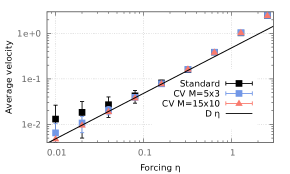
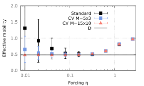
Figure 1: Linear response for the standard MC simulation (black squares) compared to the version with control variate (blue, red) and to the asymptotic response $D\eta\approx 0.48\eta$ (black line).

Correlation profiles.

The asymptotic variance of time averages for an observable $\varphi\in\mathcal{S}$ writes, using the Green–Kubo formula [37],

$$\sigma_{\varphi}^{2}=2\int_{0}^{\infty}C_{\varphi}(t)\,\differential t,\qquad C_{\varphi}(t)=\mathbb{E}[(\varphi(X_{0})-\mathbb{E}[\varphi])(\varphi(X_{t})-\mathbb{E}[\varphi])],$$

where the autocorrelation function $C_{\varphi}$ involves an expectation over all initial condition $X_{0}=(q_{0},p_{0})\in\mathcal{X}$ distributed according to the invariant probability measure $\pi_{0}$ at equilibrium, and for all realizations of the dynamics with generator $\mathcal{L}_{0}$. The integrability of $C_{\varphi}(t)$ can be guaranteed when the semi-group $\mathrm{e}^{t\mathcal{L}_{0}}$ decays sufficiently fast in ${\mathrm{L}_{n}^{\infty}}$ [42]. The function $C_{\varphi}$ is characterized by three major features explaining the value of the asymptotic variance; see Figure 2 for an illustration.

1. The first one is the amplitude of the signal $\|\varphi-\mathbb{E}[\varphi]\|_{\mathrm{L}^{2}(\pi_{0})}^{2}=C_{\varphi}(0)$ corresponding to the value of the autocorrelation at $t=0$.

2. The second one is the characteristic decay time $\tau$ of the autocorrelation, which can be related to the decay of its exponential envelope.

3. The last one is the presence of anticorrelations, which arise only for non-reversible dynamics such as Langevin dynamics.

A proper estimation of the asymptotic variance requires to compute autocorrelation profiles on a sufficiently long time interval $[0,t_{\rm deco}]$ (here $t_{\rm deco}=6$). One can check a posteriori that this time is sufficient by looking at the convergence of the cumulated autocorrelation $t\mapsto\int_{0}^{t}C_{\varphi}$ toward its limit $\frac{\sigma_{\varphi}^{2}}{2}=\int_{0}^{\infty}C_{\varphi}$ (see Appendix D for more details on the variance estimators, and the computation of error bars for these quantities).

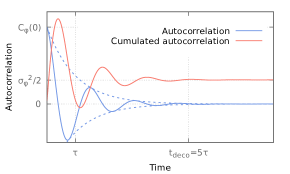
Figure 2: Illustrative autocorrelation profile. The dashed line is the exponential envelope of the correlation function.

Figure 3 compares the autocorrelation profile of the velocity with the ones for the modified observables, for two different Galerkin basis sizes $M$ and two different forcing amplitudes $\eta$. For a small forcing $\eta=0.08$ the two modified observables have an amplitude and a decorrelation time which are both much smaller than for the standard velocity. Note that the two modified observables do not exhibit any anti-correlation, contrarily to the velocity observable. The cumulated plots show that the control variates drastically reduce the asymptotic variance in this case, especially for the one based on a more accurate Galerkin approximation. For a larger value $\eta=1.28$ the modified observables have a significantly larger amplitude (i.e. $C_{\varphi}(0)$ is larger), especially in the case of a low accuracy $M$. However the decorrelation times are small and there is anti-correlation, resulting in a reasonable variance reduction in both cases.

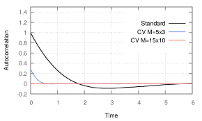
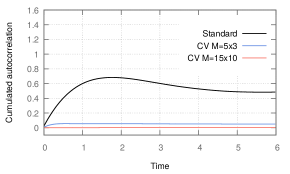
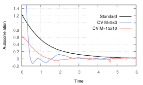
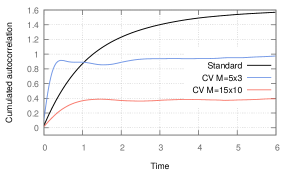
Figure 3: Left: Autocorrelation profile of the velocity compared to the one of the modified observables for two different accuracies, either for a small forcing $\eta=0.08$ (top) or a larger one $\eta=1.28$ (bottom). Right: Corresponding cumulated autocorrelations. The limit value is half the asymptotic variance of the observable.

Asymptotic variances.

Let us now compute the asymptotic variance for a whole range of Galerkin accuracies $M$ and forcing amplitudes $\eta$. The results presented in Figure 4 confirm that for a very accurate Galerkin resolution the variance of the modified observable scales as $\eta^{2}$ with the prefactor $\alpha=\left\langle\Pi_{0}AR,-\mathcal{L}_{0}^{-1}\Pi_{0}AR\right\rangle_{0}$ predicted theoretically in Theorem 2. This prefactor has been computed independently by solving (23) using a Galerkin method and plugging this approximation in (24). When the Galerkin discretization is not sufficiently accurate, the variance reaches a plateau in the region of small forcings as predicted by Theorem 4.

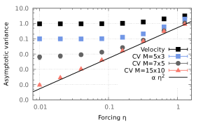
Figure 4: Asymptotic variance of the velocity (black squares) compared to its counterpart when using a control variate (blue, grey, red) and to the reduced variance (black line) predicted theoretically ($\alpha\approx 0.53$ computed with a Galerkin discretization).

4 Thermal transport in atom chains

Thermal transport in one-dimensional systems has been the topic of many investigations, both from theoretical and numerical points of view [8, 44, 15]. Determining which microscopic ingredients influence the scaling of the conductivity with respect to the length of the chain is still an active line of research. Studying numerically this scaling requires to simulate chains of thousands of particles. In these systems the temperature gradient and the thermal flux are both very small, which induces large statistical errors when estimating the conductivity. Introducing variance reduction techniques not requiring the knowledge of the invariant probability measure could alleviate (at least partly) these difficulties.

4.1 Full dynamics

4.1.1 Equations of motion

We consider a chain composed of $N$ particles interacting through a nearest-neighbor potential $v$ (see Figure 5). The evolution is dictated by a Hamiltonian dynamics and a thermalization mechanism at the boundaries, where the first and the last particles are submitted to Ornstein-Uhlenbeck processes, at temperatures $T_{\mathrm{L}}$ and $T_{\mathrm{R}}$ respectively. The unknowns are the momenta $p=(p_{n})_{1\leqslant n\leqslant N}$ of the particles and the interparticle distances $r=(r_{n})_{1\leqslant n\leqslant N-1}$. In these variables, the dynamics reads:

$$\left\{\begin{aligned} \differential r_{n}&=\frac{1}{m}(p_{n+1}-p_{n})\,\differential t,\\ \differential p_{1}&=v^{\prime}(r_{1})\,\differential t-\frac{\gamma}{m}p_{1}\differential{t}+\sqrt{2\gamma T_{\mathrm{L}}}\differential W_{t}^{L},\\ \differential p_{n}&=(v^{\prime}(r_{n})-v^{\prime}(r_{n-1}))\,\differential t,\\ \differential p_{N}&=-v^{\prime}(r_{N-1})\,\differential t-\frac{\gamma}{m}p_{N}\differential{t}+\sqrt{2\gamma T_{\mathrm{R}}}\differential W_{t}^{R},\end{aligned}\right.$$ (26)

where $m>0$ is the mass of a particle, $\gamma>0$ is the friction coefficient, $T_{\mathrm{L}}\geqslant T_{\mathrm{R}}$ and $W_{t}^{L}$, $W_{t}^{R}$ are two independent standard one-dimensional Brownian motions. Notice that the ends of the chain are free. The Hamiltonian of the system is the sum of the potential and kinetic energies:

$$H(r,p)=V(r)+\sum_{n=1}^{N}\frac{p_{n}^{2}}{2m},\quad V(r)=\sum_{n=1}^{N-1}v(r_{n}).$$

The infinitesimal generator of the dynamics (26) reads

$$\mathcal{L} =\frac{1}{m}\sum_{n=1}^{N-1}(p_{n+1}-p_{n})\partial_{r_{n}}+\sum_{n=1}^{N}(v^{\prime}(r_{n})-v^{\prime}(r_{n-1}))\partial_{p_{n}}$$

$$\quad-\frac{\gamma}{m}p_{1}\partial_{p_{1}}+\gamma T_{L}\partial_{p_{1}}^{2}-\frac{\gamma}{m}p_{N}\partial_{p_{N}}+\gamma T_{R}\partial_{p_{N}}^{2},$$

using the convention $v^{\prime}(r_{0})=v^{\prime}(r_{N})=0$.

Figure 5: Heat transport in a one-dimensional chain.

4.1.2 Properties of the dynamics

Let us recall some properties of the dynamics (26) which hold under the following assumption.

Assumption 6.

The interaction potential $v$ is $\mathcal{C}^{\infty}$ and there exist $k\geqslant 2$ and $a>0$ such that

$$\forall r_{1}\in\mathbb{R},\quad\lim_{\tau\to+\infty}\tau^{-k}v(\tau r_{1})=a|r_{1}|^{k},\quad\lim_{\tau\to+\infty}\tau^{1-k}v^{\prime}(\tau r_{1})=ka|r_{1}|^{k-1}\mathrm{sign}(r_{1}).$$

Moreover the interaction potential is not degenerate: for any $r_{1}\in\mathbb{R}$ there exists $m=m(r_{1})\geqslant 2$ such that $\partial_{m}v(r_{1})\neq 0$.

These conditions hold for the potentials we use in the numerical simulations reported in Section 4.3. When Assumption 6 holds, the dynamics admits a unique invariant probability measure $\pi$ (see [12]). This invariant probability measure is explicit when the chain is at equilibrium ($T_{\mathrm{L}}=T_{\mathrm{R}}=\beta^{-1}$), in which case it has the tensorized form

$$\pi_{\rm eq}(\differential r\,\differential p)=Z_{\beta}^{-1}\exp(-\beta\left(\frac{|p|^{2}}{2m}+V(r)\right))\,\differential r\,\differential p,$$ (27)

where $Z_{\beta}^{-1}$ is a normalization constant. Let us emphasize that the reference system considered later on in Section 4.2 is not at equilibrium. Following the framework considered in [12] (which is itself based on [55]), we consider in this section the Lyapunov functions $\mathcal{K}_{\theta}=\mathrm{e}^{\theta H}$. There exist $\theta_{*}>0$ such that $\mathcal{K}_{\theta}\subset\mathrm{L}^{2}(\pi)$ for any $\theta\in[0,\theta_{*})$. The functional spaces we use are also indexed by the continuous parameter $\theta\in[0,\theta_{*})$:

$$\mathrm{L}_{\theta}^{\infty}=\left\{\varphi\ {\rm measurable}\ \big{|}\ \|\varphi\,\mathrm{e}^{-\theta H}\|_{\mathrm{L}^{\infty}}<+\infty\right\},$$

and the space $\mathcal{S}$ is defined similarly to (12). For $\theta\in[0,\theta_{*})$, we also define the vector space $\mathrm{L}_{\theta,0}^{\infty}$ of functions of $\mathrm{L}_{\theta}^{\infty}$ with mean zero with respect to $\pi$. One can prove the exponential decay of the semi-group on the associated functional space $\mathrm{L}_{\theta,0}^{\infty}$ (see [12]): for any $\theta\in[0,\theta_{*})$, there exist $C,\lambda>0$ such that, for any $\varphi\in\mathrm{L}_{\theta,0}^{\infty}$,

$$\forall t\geqslant 0,\quad\|\mathrm{e}^{t\mathcal{L}}\varphi\|_{\mathrm{L}_{\theta}^{\infty}}\leqslant C\mathrm{e}^{-\lambda t}\|\varphi\|_{\mathrm{L}_{\theta}^{\infty}}.$$

This implies that $\mathcal{L}$ is invertible on $\mathrm{L}_{\theta,0}^{\infty}$, and that its inverse is bounded.

Validity of Assumptions 1 and 2.

Assumption 1 holds true since there exist a unique invariant probability measure with positive density with respect to the Lebesgue measure, and the generator of the dynamics is hypoelliptic [12, 33, 55]. The first part of Assumption 2 is also satisfied for $\theta\in[0,\theta_{*})$. Note that at equilibrium ($T_{\mathrm{L}}=T_{\mathrm{R}}=\beta^{-1}$) the invariant probability measure is explicit and $\theta^{*}=\beta/2$. The product of two Lyapunov functions $\mathcal{K}_{\theta}$ and $\mathcal{K}_{\theta^{\prime}}$ is in a Lyapunov space only if $\theta+\theta^{\prime}<\theta_{*}$, so the second part of Assumption 2 is not satisfied.

4.1.3 Heat flux and conductivity

When studying heat transport in atom chains the typical quantity of interest is the thermal flux through the chain:

$$\forall n\in[1,N-1],\quad j_{n}(r,p)=-\frac{p_{n}+p_{n+1}}{2}v^{\prime}(r_{n}),$$ (28)

see for example the review [43] on thermal transport in low-dimensional lattices for further background material. We also make use of the two boundary elementary fluxes:

$$j_{0}(r,p)=\frac{\gamma}{m}\left(T_{\mathrm{L}}-\frac{p_{1}^{2}}{m}\right),\qquad j_{N}(r,p)=\frac{\gamma}{m}\left(\frac{p_{N}^{2}}{m}-T_{\mathrm{R}}\right).$$ (29)

The definition of the elementary fluxes $j_{n}$ is motivated by the local energy balance, centered on particle $n$:

$$\forall n\in[1,N],\quad\mathcal{L}\varepsilon_{n}=j_{n-1}-j_{n},\qquad\varepsilon_{n}(r,p)=\frac{v(r_{n-1})}{2}+\frac{p_{n}^{2}}{2m}+\frac{v(r_{n})}{2}.$$ (30)

The quantity $\mathcal{L}\varepsilon_{n}$ is of mean zero since it is in the image of the generator. Therefore the elementary fluxes $j_{n}$ all have the same stationary values:

$$\mathbb{E}_{\pi}[j_{0}]=\mathbb{E}_{\pi}[j_{1}]=\cdots=\mathbb{E}_{\pi}[j_{N}].$$ (31)

Any linear combinations of such fluxes, namely

$$J_{\lambda}=\sum_{n=0}^{N}\lambda_{n}j_{n},\qquad\sum_{n=0}^{N}\lambda_{n}=1,$$ (32)

has the same stationary value. The most common choice is the spatial mean

$$\widetilde{R}=\frac{1}{N-1}\sum_{n=1}^{N-1}j_{n}.$$ (33)

We call the latter observable "standard heat flux" in the sequel. Notice that it does not depend on the boundary fluxes $j_{0}$ and $j_{N}$. The linear response of $\widetilde{R}$ (or of any flux $J_{\lambda}$) with respect to the temperature gradient $\frac{T_{\mathrm{L}}-T_{\mathrm{R}}}{N-1}$ defines the effective conductivity:

$$\kappa=\frac{N-1}{T_{\mathrm{L}}-T_{\mathrm{R}}}\mathbb{E}_{\pi}[\widetilde{R}],$$ (34)

which is here the transport coefficient of interest. There exist infinitely many observables having the same expectation as $\widetilde{R}$, see (32) for example. Let us first discuss the choice of observable for the heat flux, before trying to reduce its variance by constructing a control variate.

Asymptotic variance of the heat fluxes at equilibrium.

The chain is supposed to be at equilibrium in all this paragraph ($T_{\mathrm{L}}=T_{\mathrm{R}}=\beta^{-1}$). The conclusions remain unchanged for nonequilibrium systems when $T_{\mathrm{L}}-T_{\mathrm{R}}$ is small since the results are only perturbed to first order with respect to this quantity. In the remainder of Section 4, an index ’eq’ refers to the equilibrium dynamics and to the equilibrium invariant probability measure $\pi_{\rm eq}$. In this setting the asymptotic variance $\sigma_{\widetilde{R},{\rm eq}}^{2}$ for the standard heat flux $\widetilde{R}$ is not smaller than the one associated with any elementary flux $(j_{n})_{1\leqslant n\leqslant N-1}$. These two variances are in fact equal, as made precise in the following proposition (similar in spirit to Remark 6).

Proposition 1.

Consider an observable $\varphi\in\mathcal{S}$ and a function $U\in\mathcal{S}$ which does not depend on $p_{1}$ and $p_{N}$. Then adding $\mathcal{L}U$ to the observable does not modify the variance:

$$\sigma_{\varphi+\mathcal{L}U,{\rm eq}}^{2}=\sigma_{\varphi,{\rm eq}}^{2}.$$ (35)

Proof.

At equilibrium, the invariant probability measure $\pi_{\rm eq}$ is explicit. The symmetric part of the generator can then be computed and it corresponds to the fluctuation-dissipation part of the process:

$$\frac{1}{2}(\mathcal{L}+\mathcal{L}^{*})=\mathcal{L}_{\mathrm{FD}}:=-\frac{\gamma}{\beta}\left(\partial_{p_{1}}^{*}\partial_{p_{1}}+\partial_{p_{N}}^{*}\partial_{p_{N}}\right),$$ (36)

where adjoints are considered on ${\mathrm{L}^{2}(\pi_{\rm eq})}$. When $U$ does not depend on $p_{1}$ nor $p_{N}$, it holds $\mathcal{L}_{\mathrm{FD}}U=0$. The claimed result then follows from Lemma 2. ∎

The equality (35) is perturbed by terms of order $T_{\mathrm{L}}-T_{\mathrm{R}}$ for out of equilibrium dynamics according to linear response theory. Upon taking for $U$ a linear combination of the energies $(\varepsilon_{n})_{2\leqslant n\leqslant N-1}$, we directly obtain, thanks to (30), that all the fluxes of the form (32) which do not depend on the boundary fluxes ($\lambda_{0}=\lambda_{N}=0$) share the same asymptotic variance at equilibrium; in particular

$$\forall 1\leqslant n\leqslant N-1,\quad\sigma_{j_{n},{\rm eq}}^{2}=\sigma_{\widetilde{R},{\rm eq}}^{2}.$$ (37)

Remark 7.

Linear response theory indicates that the previous asymptotic variances are related to the conductivity through the Green–Kubo formula [37]:

$$\sigma_{\widetilde{R},{\rm eq}}^{2}=\frac{2\kappa}{\beta^{2}(N-1)}.$$ (38)

We show in Appendix B.2 that, in this equilibrium situation, the variance of the two boundary fluxes $j_{0}$ and $j_{N}$ is also related to the conductivity as:

$$\sigma_{j_{0},{\rm eq}}^{2}=\frac{\gamma}{m\beta^{2}}-\frac{2\kappa}{\beta^{2}(N-1)},\qquad\sigma_{j_{N},{\rm eq}}^{2}=\frac{\gamma}{m\beta^{2}}-\frac{2\kappa}{\beta^{2}(N-1)}.$$ (39)

Apart from special cases such as integrable systems (as the harmonic system considered in Appendix B.4), we generically observe numerically that $\frac{\kappa(N)}{N-1}\xrightarrow[N\to\infty]{}0$. The boundary fluxes therefore have (asymptotically in $N$) a larger variance than bulk fluxes. Since the variances are perturbed to first order in $T_{\mathrm{L}}-T_{\mathrm{R}}$ in nonequilibrium situations, the same conclusion holds for temperature differences which are not too large.

In the next section we construct a modified observable by adding a control variate to the reference observable $R=\frac{1}{2}(j_{0}+j_{N})$. This particular heat flux does not depend on the potential energy function $v$, which simplifies the computation of the control variate (see Appendix B.4). In Appendix B.1 we prove using Proposition 1 that, at equilibrium, the asymptotic variance of the resulting modified observable does not depend on the choice of the reference observable $R$.

4.2 Simplified dynamics and control variate

We split the interaction potential into a harmonic part with parameters $\hat{\omega}>0$ and $\hat{r}\in\mathbb{R}$, and an anharmonic part $w$:

$$v(r_{1})=v_{0}(r_{1})+w(r_{1}),\qquad v_{0}(r_{1})=\frac{1}{2}m\hat{\omega}^{2}(r_{1}-\hat{r})^{2}.$$ (40)

The potential energy is then decomposed as

$$V(r)=V_{0}(r)+W(r),\qquad V_{0}(r)=\sum_{n=1}^{N-1}v_{0}(r_{n}),\qquad W(r)=\sum_{n=1}^{N-1}w(r_{n}).$$

Following the general strategy outlined in Section 2 we decompose the generator as

$$\mathcal{L}=\mathcal{L}_{0}+\widetilde{\mathcal{L}},$$

where $\mathcal{L}_{0}$ is the generator of the harmonic chain corresponding to the harmonic interaction potential $v_{0}$ and $\widetilde{\mathcal{L}}$ is the generator of the anharmonic perturbation:

$$\widetilde{\mathcal{L}}=\sum_{n=1}^{N}\left(w^{\prime}(r_{n})-w^{\prime}(r_{n-1})\right)\partial_{p_{n}},$$

with the same convention $w^{\prime}(r_{0})=w^{\prime}(r_{N})=0$ as for the potential $v$. We simplify the Poisson problem for the optimal control variate

$$-\mathcal{L}\Phi=R-\mathbb{E}[R],$$

into the harmonic Poisson problem

$$-\mathcal{L}_{0}{\Phi_{0}}=R-\mathbb{E}_{0}[R].$$ (41)

Note that the observable $R$ does not depend on the potential, contrarily to other heat fluxes such as $\widetilde{R}$ in (33), so that the right hand side of the Poisson equation needs not be changed when looking for an approximate control variate. Equation (41) can be solved analytically for ${\Phi_{0}}$. In Appendix B.4 we show that

$$\mathbb{E}_{0}[R] =\frac{\nu^{2}}{1+\nu^{2}}\frac{\gamma(T_{\mathrm{L}}-T_{\mathrm{R}})}{2m},$$ (42)

$${\Phi_{0}}(r,p) =\frac{m}{2\gamma\left(1+\nu^{2}\right)}\left[-\hat{\omega}^{2}\sum_{n=1}^{N-1}(r_{n}-\hat{r})(p_{n}+p_{n+1})+\frac{\gamma}{2m^{2}}\left(p_{N}^{2}-p_{1}^{2}\right)\right]+C,$$

where $\nu=\frac{m\hat{\omega}}{\gamma}$ and $C\in\mathbb{R}$ is such that $\mathbb{E}_{0}[{\Phi_{0}}]=0$. The modified observable is therefore

$$\quad(R+\mathcal{L}{\Phi_{0}})(r,p)=\mathbb{E}_{0}[R]+\widetilde{\mathcal{L}}{\Phi_{0}}(r,p)$$ (43)

$$=\frac{1}{2(1+\nu^{2})}\left[\nu\hat{\omega}(T_{\mathrm{L}}-T_{\mathrm{R}})-\nu\hat{\omega}\sum_{n=1}^{N-1}(r_{n}-\hat{r})\left(w^{\prime}(r_{n+1})-w^{\prime}(r_{n-1})\right)-\left(\frac{p_{1}}{m}w^{\prime}(r_{1})+\frac{p_{N}}{m}w^{\prime}(r_{N-1})\right)\right]$$

$$=\frac{1}{2(1+\nu^{2})}\left[\nu\hat{\omega}(T_{\mathrm{L}}-T_{\mathrm{R}})-\sum_{n=1}^{N-1}\left(\widetilde{v}_{n+1}(r,p)-\widetilde{v}_{n-1}(r,p)\right)w^{\prime}(r_{n})\right],$$

where

$$\widetilde{v}_{n}(r,p)=\left\{\begin{array}[]{cl}-\frac{p_{1}}{m}&\mbox{if}\quad n=0,\\ -\nu\hat{\omega}(r_{n}-\hat{r})&\mbox{if}\quad 1\leqslant n\leqslant N-1,\\ \frac{p_{N}}{m}&\mbox{if}\quad n=N.\end{array}\right.$$

Notice that, by construction, this observable is constant when the chain is harmonic (i.e. $w=0$).

Harmonic fitting.

For a given pair potential $v=v(r)$, there is some freedom in the decomposition (40), namely the choice of the parameters $\hat{\omega}$ and $\hat{r}$. The optimal choice would be such that the variance of the modified observable (43) is minimal, but this condition is not practical. A possible (and simpler) heuristic is to choose these coefficients in order to minimize the $\mathrm{L}^{2}(\pi_{\rm eq})$ norm of the anharmonic force $-\nabla W$ at equilibrium, namely when $T_{\mathrm{L}}=T_{\mathrm{R}}=\beta^{-1}$. In view of the tensorized form (27) of the invariant probability measure at equilibrium,

$$\|\nabla W(r)\|_{\rm eq}^{2}=(N-1)z_{\beta}^{-1}\int_{\mathbb{R}}\left(v^{\prime}(r_{1})-m\hat{\omega}^{2}(r_{1}-\hat{r})\right)^{2}\,\mathrm{e}^{-\beta v(r_{1})}\differential r_{1},$$

where $z_{\beta}=\int_{\mathbb{R}}\mathrm{e}^{-\beta v(r_{1})}\differential r_{1}$. Therefore the minimization problem defining $\hat{r}$ and $\hat{\Omega}=m\hat{\omega}^{2}$ writes

$$\operatorname*{\arg\!\min}_{\hat{\omega},\hat{r}}\int_{\mathbb{R}}\left(v^{\prime}(r_{1})-\hat{\Omega}(r_{1}-\hat{r})\right)^{2}\,\mathrm{e}^{-\beta v(r_{1})}\differential r_{1}.$$ (44)

There exists a minimizer $(\hat{r},\hat{\Omega})$ since the function to be minimized is continuous and coercive; uniqueness is proved in Appendix B.3. Define the moments of the marginal measure for inter-particle distances as:

$$\mathcal{M}_{k}=\int_{\mathbb{R}}r_{1}^{k}\mathrm{e}^{-\beta v(r_{1})}\differential r_{1}.$$

The Euler-Lagrange equation associated with (44) provides the expression of the minimizer (see Appendix B.3):

$$\hat{r}=\frac{\mathcal{M}_{1}}{\mathcal{M}_{0}},\qquad\hat{\Omega}=m\hat{\omega}^{2}=\beta^{-1}\frac{\mathcal{M}_{0}^{2}}{\mathcal{M}_{0}\mathcal{M}_{2}-\mathcal{M}_{1}^{2}},$$ (45)

where, by the Cauchy-Schwarz inequality, $\mathcal{M}_{0}\mathcal{M}_{2}-\mathcal{M}_{1}^{2}>0$ for any continuous potential $v$ which is not constant.

Validity of Assumptions 3 to 5.

The standard way to verify Assumption 3 would be to show that the coefficients in the Lyapunov condition exhibited in [12] depend continuously on perturbations of the potential $v$. This is not straightforward, especially if the exponent $k$ introduced in Assumption 6 is discontinuous with the perturbation amplitude at $\eta=0$ (which corresponds to the harmonic chain). For example, for the FPU potential (46), $k=2$ for the harmonic chain ($\eta=0$) and $k=4$ for $\eta>0$. We show that Assumption 4 holds under Assumption 6 in Appendix B.5. Moreover it is clear that $\mathcal{S}$ is stable by $\widetilde{\mathcal{L}}$. A simple computation shows that $\pi_{0}$ is a Gaussian probability measure, which implies that $\widetilde{\mathcal{L}}^{*}\mathbf{1}\in{\mathrm{L}^{2}(\pi_{0})}$. Therefore Assumption 5 holds as well.

4.3 Numerical results

We consider a Fermi-Pasta-Ulam (FPU) potential

$$v(r_{1})=\frac{a}{2}r_{1}^{2}+\frac{b}{3}r_{1}^{3}+\frac{c}{4}r_{1}^{4},$$ (46)

where $c=\frac{b^{2}}{3a}$ is such that $v^{\prime\prime}(r_{1})=a+2br_{1}+3cr_{1}^{2}=\frac{1}{a}(a+br_{1})^{2}$ is positive except at a single point where it vanishes. This choice makes the potential both asymmetric and convex. Symmetric potentials indeed exhibit special behaviors [61], whereas we want to be as general as possible. On the other hand, non-convex potentials are not typical in the literature on the computation of thermal conduction in one-dimensional chains. In the following we fix $a=1$ and vary $b$ only. The parameters $\hat{r}$ and $\hat{\omega}$ are given by (45), where the moments $\mathcal{M}_{k}$ are computed using one-dimensional numerical quadratures.

The system is simulated for a time $T=10^{8}$ with time steps $\Delta t=10^{-2}$, and with $m=\gamma=1$. The atom chain is simulated either at equilibrium with $T_{\mathrm{L}}=T_{\mathrm{R}}=2$, or for $T_{\mathrm{L}}=3$ and $T_{\mathrm{R}}=1$. The dynamics is discretized using a Geometric Langevin Algorithm scheme as in (25). The estimator of the asymptotic variance is made precise in Appendix D. The decorrelation time is set to $t_{\rm deco}=3N$ for the standard flux $R$ and to $t_{\rm deco}=32$ for the modified observable.

We plot in Figure 6 the autocorrelation profiles of the heat flux for a chain of size $N=128$ at equilibrium, for two different anharmonicities. Let us comment this picture in greater detail. The results first show that the chosen decorrelation time $t_{\rm deco}$ is sufficiently large. Similar plots were used to check this is also the case for all the range of anharmonicities $b$ and numbers of particles $N$ we consider. They can also be used to understand the eventual variance reduction granted by the control variate (42). For a small anharmonicity $b=0.08$ we see that the asymptotic variance, which is twice the limit of the cumulated autocorrelation (right plot) is greatly reduced for two reasons. First, the signal amplitude, which is related to the autocorrelation value at $t=0$ (left plot), is slightly smaller, and (right plot) the contribution of the times $0\leqslant t\leqslant 2$ is twice smaller for the modified flux. Second, and that is the actual reason for the variance reduction, there is anticorrelation for $2\leqslant t\leqslant 5$. For a larger anharmonicity it appears that the amplitude of the modified observable is much larger, but this is compensated by a long-time anticorrelation. The resulting asymptotic variance of the modified flux is slightly smaller than the one of the standard flux. The plots are essentially the same out of equilibrium, when $T_{\mathrm{L}}=3$ and $T_{\mathrm{R}}=1$ (numerical results not presented here).

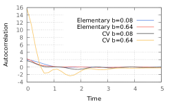
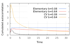
Figure 6: Comparison of results obtained either with the elementary flux $j_{n}$ (28) or with the modified observable (43), for two different anharmonicities $b=0.08,0.64$, and for a chain of $N=128$ particles at equilibrium. Left: Autocorrelation profile. Right: Cumulated autocorrelation $t\mapsto\int_{0}^{t}C$ at longer times.

The asymptotic variances, with associated error bars (see Appendix D), are plotted on Figure 7 for a whole range of anharmonicities $b$ and numbers of particles $N$. The two left plots are at equilibrium ($T_{\mathrm{L}}=T_{\mathrm{R}}=2$) while the two right plots are out of equilibrium ($T_{\mathrm{L}}=3$ and $T_{\mathrm{R}}=1$). We check that the variances are extremely similar in both cases, which is expected by linear response theory. We observe that the asymptotic variance of the modified flux scales as $b^{2}$ for $b\ll 1$, as expected from Theorem 2, providing an excellent variance reduction in this case. Note that, in the limit $b\to 0$, the variance of the standard flux tends to $\frac{\gamma\nu^{2}}{m\beta^{2}(1+\nu^{2})}=2$ (since $\nu=\frac{m\omega}{\gamma}=1$ here), which is the theoretical value predicted at equilibrium in view of the expression of the mean flux for a harmonic chain (see Equations (42), (38), and (34)). The modified flux can sometimes have a larger variance than the standard one, for example in the regime $b=\mathrm{O}(1)$ and $N$ large. Note that for the particular choice $\hat{\omega}=0$ the modified flux is $\frac{1}{2}(j_{1}+j_{N-1})$, which has the same asymptotic variance as the standard flux $\widetilde{R}$ according to (37). Therefore, for any set of parameters, there exist an optimal choice of the coefficients $\hat{\omega},\hat{r}$ providing a modified flux whose asymptotic variance is smaller or equal to its counterpart without control variate. In the present application these two coefficients are instead chosen according to the heuristic (45), leading to a degradation of the asymptotic variance in certain cases.

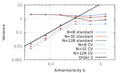
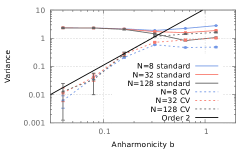
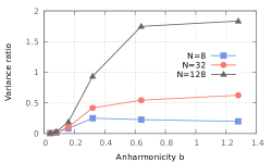
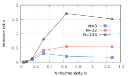
Figure 7: Comparison of variances for the standard and modified fluxes. The reported variance ratio corresponds to the modified variance divided by the standard one. Left: Chain at equilibrium ($T_{\mathrm{L}}=T_{\mathrm{R}}=2$). Right: Chain out of equilibrium ($T_{\mathrm{L}}=3$ and $T_{\mathrm{R}}=1$).

5 Solvated dimer under shear

A solvated dimer is a pair of bonded particles in a bath constituted of many other particles. It serves as a prototypical model of a molecule in solvent (e.g. peptide in water). This model has been used in the context of free energy computations [41]. We apply to this system an external shearing force as in [32], also coined sinusoidal transverse field in the physics literature (see [66, Section 9.1] and [18, 65]), so that the invariant measure of the system is not known. A typical question is the influence of the shear force on the average bond length of the dimer.

5.1 Full dynamics

We consider $N$ particles in a two-dimensional box of length $L$ with periodic boundary conditions, with positions $q=(q_{1},\cdots,q_{N})\in\mathcal{D}=(L\mathbb{T})^{2N}$. Two of these particles, with positions $q_{1}$ and $q_{2}$, form a dimer whereas the other $N-2$ particles, with positions $q_{3},\cdots,q_{N}$, constitute the solvent. The potential energy of the system is composed of three parts:

$$V(q) =v(|q_{1}-q_{2}|)+\sum_{i\in\{1,2\}}\sum_{j=3}^{N}v_{\rm sol}(|q_{i}-q_{j}|)+\sum_{3\leqslant i<j\leqslant N}v_{\rm sol}(|q_{i}-q_{j}|)$$

$$=:V_{\rm dim}(q)+V_{\rm inter}(q)+V_{\rm sol}(q),$$

where $V_{\rm dim}$ is the potential energy of the dimer, $V_{\rm inter}$ is the interaction energy between the dimer and the solvent and $V_{\rm sol}$ is the potential energy of the solvent. The two particles forming the dimer interact via a double-well potential: denoting by $r=|q_{1}-q_{2}|$ the bond length,

$$v(r)=h\left[1-\left(\frac{r-r_{0}}{\Delta r}\right)^{2}\right]^{2},$$ (47)

where $r_{0}$, $\Delta r>0$ (see Figure 8, Left). The potential $v$ presents two minima: one associated with a compact state of length $r=r_{0}-\Delta r$ and one associated with a stretched state of length $r=r_{0}+\Delta r$. These minima are separated by a potential barrier of height $h$. The particles of the solvent interact both with the other particles of the solvent and the particles of the dimer through a purely repulsive potential. In the following we consider two types of potentials with compact support (see Figure 8, Right): a soft repulsion potential (used in [25] for example)

$$\forall r>0,\quad v_{\rm sol}(r)=\varepsilon\left(1-\frac{r}{r_{\rm cut}}\right)^{2}\mathds{1}_{r\leqslant r_{\rm cut}},$$ (48)

where $\varepsilon,r_{\rm cut}>0$; and a singular Coulomb-like potential:

$$\forall r>0,\quad v_{\rm sol}(r)=\varepsilon\left(\frac{\frac{1}{\sqrt{r}}-\frac{1}{\sqrt{r_{\rm cut}}}}{\frac{1}{\sqrt{\sigma}}-\frac{1}{\sqrt{r_{\rm cut}}}}\right)^{2}\mathds{1}_{\rm r<r_{\rm cut}}=\varepsilon\frac{\sigma}{r}\left(\frac{1-\sqrt{\frac{r}{r_{\rm cut}}}}{1-\sqrt{\frac{\sigma}{r_{\rm cut}}}}\right)^{2}\mathds{1}_{r\leqslant r_{\rm cut}}.$$ (49)

This potential behaves like $\frac{1}{r}$ for $r\to 0$, reaches the value $\varepsilon$ at $r=\sigma$ and vanishes at $r=r_{\rm cut}$,where its derivative also vanishes. Note that we recover the Coulomb potential $\varepsilon\frac{\sigma}{r}$ in the limit $r_{\rm cut}\to+\infty$.

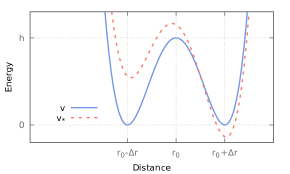
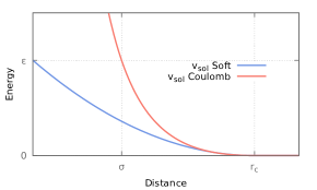
Figure 8: Pairwise potentials for the solvated dimer model. Left: Potential for the dimer and associated free energy in vacuum (see (52)). Right: Potentials for the solvent interaction.

The system is driven out of equilibrium by a shearing force of amplitude $\nu$. More precisely, a particle located at a position $(q_{i,x},q_{i,y})$ experiences the force [32, 66]:

$$(0,f(q_{i,x}))=\left(0,\nu\sin(2\pi\frac{q_{i,x}}{L})\right).$$

This force is in the $y$ direction and depends only on $x$. It therefore induces a non-equilibrium forcing since it is not of gradient type. We are interested in computing the mean length of the dimer $R(q,p)=|q_{1}-q_{2}|$ as a function of this external forcing. The corresponding average is denoted by $\mathbb{E}[|q_{1}-q_{2}|]$.

For simplicity we study the overdamped dynamics associated with $V$, but everything can be adapted to the Langevin case. Since the space $\mathcal{D}$ is compact and the noise in the dynamics is non degenerate, there exist a unique invariant probability measure $\pi$ by the Doeblin condition when the potentials under consideration are smooth. This invariant measure depends on $\nu$, and is not explicit. Proving a similar result for singular potentials such as the Coulomb-like potential (49) would require more work.

The generator can be decomposed as:

$$\mathcal{L} =-\nabla V(q)\cdot\nabla+\beta^{-1}\Delta+\nu\sum_{i=1}^{N}f(q_{i,x})\partial_{q_{i,y}}=\mathcal{L}_{\rm dim}+\mathcal{L}_{\rm inter}+\mathcal{L}_{\rm sol}+\nu\mathcal{L}_{\mathrm{pert}},$$

where

$$\mathcal{L}_{\rm dim} =\sum_{i=1,2}\left(-\nabla_{q_{i}}V_{\rm dim}(q)\cdot\nabla_{q_{i}}+\beta^{-1}\Delta_{q_{i}}\right), \qquad\mathcal{L}_{\rm inter} =-\nabla V_{\rm inter}(q)\cdot\nabla,$$

$$\mathcal{L}_{\rm sol} =\sum_{i=3}^{N}\left(-\nabla_{q_{i}}V_{\rm sol}(q)\cdot\nabla_{q_{i}}+\beta^{-1}\Delta_{q_{i}}\right), \qquad\mathcal{L}_{\mathrm{pert}} =\sum_{i=1}^{N}f(q_{i,x})\partial_{q_{i,y}}.$$

Note that $\mathcal{L}_{\rm dim}$ is the generator of the dynamics of the dimer at equilibrium in vacuum and $\mathcal{L}_{\rm sol}$ is the generator of the dynamics of the solvent at equilibrium and without dimer.

5.2 Simplified dynamics and control variate

We consider the following reference Poisson equation where the system is at equilibrium and the interaction between the dimer and the solvent has been switched off:

$$-\mathcal{L}_{0}{\Phi_{0}}=R-\mathbb{E}_{0}[R],$$ (50)

where

$$\mathcal{L}_{0}=\mathcal{L}_{\rm dim}+\mathcal{L}_{\rm sol}.$$

Let us show that this equation admits a solution ${\Phi_{0}}$ depending only on the length $|q_{1}-q_{2}|$ of the dimer. In order to highlight the dependence on the dimension of the underlying space, let us denote by $d=2$ this dimension. Assume that ${\Phi_{0}}$ is defined for any $q\in(L\mathbb{T})^{dN}$ by ${\Phi_{0}}(q)=\frac{1}{2}\psi(|q_{1}-q_{2}|)$ for some smooth function $\psi$. The Laplacian of ${\Phi_{0}}$ can be rewritten using spherical coordinates as:

$$\Delta{\Phi_{0}}(q)=\psi^{\prime\prime}(|q_{1}-q_{2}|)+\frac{d-1}{|q_{1}-q_{2}|}\psi^{\prime}(|q_{1}-q_{2}|),$$ (51)

where $d=2$ is the dimension of the underlying physical space. We obtain by substituting ${\Phi_{0}}$ into (50) that $\psi$ satisfies the following one-dimensional differential equation:

$$\forall r>0,\quad v_{*}^{\prime}(r)\psi^{\prime}(r)-\beta^{-1}\psi^{\prime\prime}(r) =r-r^{*},$$ (52)

where $v_{*}(r)=v(r)-\frac{d-1}{\beta}\ln(r)$ and $r^{*}=\mathbb{E}_{*}[r]$ is the expectation of the length $r$ with respect to the probability measure $\pi_{*}(\differential r)=Z_{*}^{-1}\mathrm{e}^{-\beta v_{*}(r)}\,\differential r$. Note the additional term $-\frac{d-1}{\beta}\ln(r)$ in the expression of $v_{*}$ coming from (51), which can be interpreted as an entropic contribution.

Let us first discuss the well-posedness of (52). The double-well potential (47) considered here is such that $v_{*}$ is a bounded perturbation of a convex function. Therefore $\pi_{*}(\differential r)$ satisfies a log-Sobolev inequality and thus a Poincaré inequality by the Holley-Stroock theorem [29] and the Bakry-Emery criterion [5]. This implies that the one-dimensional Poisson problem (52) then admits a unique solution in

$$\mathrm{H}^{1}(\pi_{*})\cap\mathrm{L}_{0}^{2}(\pi_{*})=\left\{\varphi\in H^{1}(\pi_{*}),\ \int_{0}^{+\infty}\varphi\,\differential\pi_{*}=0\right\}$$

by the Lax-Milgram theorem for the variational formulation:

$$\forall u\in\mathrm{H}^{1}(\pi_{*})\cap\mathrm{L}_{0}^{2}(\pi_{*}),\quad\beta^{-1}\int_{0}^{\infty}\psi^{\prime}(r)u^{\prime}(r)\,\pi_{*}(\differential r)=\int_{0}^{\infty}(r-r_{*})u(r)\,\pi_{*}(\differential r).$$

We discuss precisely in Appendix C how we numerically solve (52). Knowing the solution $\psi$, the corresponding modified observable then writes

$$(R+\mathcal{L}{\Phi_{0}})(q) =|r_{12}|+\beta^{-1}\psi^{\prime\prime}(|r_{12}|)$$

$$+\left[\frac{1}{2}\big{(}\nabla_{q_{1}}V(q)-\nabla_{q_{2}}V(q)-\nu(f(q_{1,x})-f(q_{2,x}))e_{y}\big{)}\cdot\frac{r_{12}}{|r_{12}|}+\frac{d-1}{\beta|r_{12}|}\right]\psi^{\prime}(|r_{12}|),$$

where $r_{12}=q_{2}-q_{1}$ and $e_{y}=(0,1)$. Note that $\nabla_{q_{1}}V$ and $\nabla_{q_{2}}V$ are the forces that apply on particles $1$ and $2$ respectively, which depend also on the solvent variables.

5.3 Numerical results

We simulate a system of $N=64$ particles in $d=2$ dimensions, using periodic boundary conditions. We fix $L=8$ (so that the particle density is $1$), and $\beta=1$. The parameters of the potentials are set to $r_{\rm cut}=2.5$, $\varepsilon=1$, $h=1$, $r_{0}=3$ and $\Delta r=1$ (see Figure 8). For the finite difference method used to solve the Poisson equation (52) we use a mesh size $\Delta r=10^{-3}$ on an interval $[0,r_{\rm max}]$ with $r_{\rm max}=10$ (see Appendix C).

The influence of the shearing on the average dimer length is plotted on Figure 9. We see that a shear force of amplitude $\nu=1$ increases the mean length by roughly $1\%$, and that the response of the mean length to the nonequilibrium forcing is of order $2$. The response is small thus difficult to estimate accurately, hence the need for control variates to alleviate this issue.

In the case of an unsolvated dimer, Figure 10 (Left) shows that the variance of the modified observable scales like $\nu^{2}$, as predicted by Theorem 2. Note that in the limit $\nu\to 0$ the modified observable is the constant $\mathbb{E}_{0}[R]=r_{*}$, which is computed by a numerical quadrature, so that the variance converges to zero.

When the solvent interacts with the dimer the variance of the modified observable plateaus at a certain value when $\nu\to 0$ , as expected from Theorem 4. For the soft potential (48), the variance scales like $\nu$ for a forcing amplitude of order $1$, which is expected from Theorem 4 (see Figure 10, Right). The variance stabilizes at a value which is ten times smaller than the initial one. For the Coulomb-like potential the influence of the solvent on the dimer is stronger and the control variate does not perform as well, as seen on Figure 10 (Bottom). For a small shearing the variance is however reduced by a factor 4.

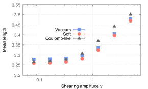
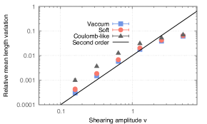
Figure 9: Left: Mean length of a dimer, either unsolvated (in vacuum) or in a solvent with soft or Coulomb-like potential. Right: Relative variation of this mean length induced by the shearing. The solid line represents the reference scaling $\nu^{2}$.

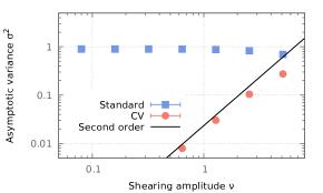
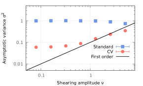
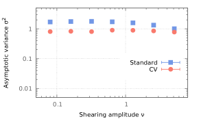
Figure 10: Asymptotic variance of the length of the dimer, with or without control variate. Left: Unsolvated dimer. Right: Solvent with the soft potential (48). Bottom: Solvent with the Coulomb-like potential (49).

Generalization.

The variance reduction strategy discussed here can be easily adapted to similar systems. For example Langevin dynamics can be treated by replacing (52) by a two-dimensional PDE where the variables are the dimer length and the radial part of the momentum associated to this length. The Poisson equation should then be solved using a Galerkin approximation similar to what is done Section 3. One could also consider a solvated molecule more complex than a dimer. In this case the PDE (52) would be posed in several dimensions and thus become rapidly impossible to solve in practice. In general one has to reduce the system to a few relevant variables corresponding to a simplified Poisson equation in order to use the control variate approach developed here. This is connected to coarse-graining, i.e. finding a few (nonlinear) functions of the degrees of freedom providing some macroscopic information on the system – think of identifying an appropriate molecular backbone for proteins. An alternative route, which does not require an a priori physical knowledge of the system, would be to resort to greddy methods [50, 64, 11, 19]. If the system possesses in addition a specific symmetry or structure, one can make profit of dedicated tensor formats [26] as done for the Schrödinger equation in [68]. This approach would be particularly adapted when studying an isotropic system composed of identical particles for example. Let us also mention recent advances on the resolution of Poisson equations based on deep convolutional neural networks [59, 4], which offer the promise of a better scalability with respect to the dimension of the system.

Appendix A Proofs of Theorems 2 and 4

Let us first prove Theorem 2, and deduce Theorem 4 in a second step. We suppose in all this section that Assumptions 1 to 5 hold true. The norm and scalar product indexed by $\eta$ correspond to the canonical ones on ${\mathrm{L}^{2}(\pi_{\eta})}$. We start by giving a useful technical result.

Lemma 1.

For any $\eta_{*}>0$ and $n\in\mathbb{N}$, there exists $C_{n,\eta_{*}}\in\mathbb{R}_{+}$ such that, for any $|\eta|\leqslant\eta_{*}$,

$$\forall\varphi\in{\mathrm{L}_{n}^{\infty}},\quad\left|\mathbb{E}_{\eta}[\varphi]-\mathbb{E}_{0}[\varphi]\right|\leqslant C_{n,\eta_{*}}\,|\eta|\,\|\varphi\|_{\mathrm{L}_{n}^{\infty}}.$$

Proof.

For any $\psi\in\mathcal{S}$,

$$\mathbb{E}_{0}[\mathcal{L}_{\eta}\psi]=\eta\mathbb{E}_{0}[\widetilde{\mathcal{L}}\psi],$$

so that, for a given $\varphi\in\mathcal{S}$, the previous equality applied to $\psi={\mathcal{L}_{\eta}^{-1}}\Pi_{\eta}\varphi$ leads to

$$\mathbb{E}_{0}[\Pi_{\eta}\varphi]=\eta\mathbb{E}_{0}[\widetilde{\mathcal{L}}{\mathcal{L}_{\eta}^{-1}}\Pi_{\eta}\varphi]=\eta\left\langle\widetilde{\mathcal{L}}{\mathcal{L}_{\eta}^{-1}}\Pi_{\eta}\varphi,\mathbf{1}\right\rangle_{0}=\eta\left\langle{\mathcal{L}_{\eta}^{-1}}\Pi_{\eta}\varphi,\widetilde{\mathcal{L}}^{*}\mathbf{1}\right\rangle_{0}.$$

Since $\mathbb{E}_{0}[\Pi_{\eta}\varphi]=\mathbb{E}_{0}[\varphi]-\mathbb{E}_{\eta}[\varphi]$ and $|\varphi|\leqslant\|\varphi\|_{\mathrm{L}_{n}^{\infty}}\mathcal{K}_{n}$, we obtain

$$\left|\mathbb{E}_{\eta}[\varphi]-\mathbb{E}_{0}[\varphi]\right|\leqslant|\eta|\big{\|}{\mathcal{L}_{\eta}^{-1}}\big{\|}_{\mathcal{B}(\Pi_{\eta}{\mathrm{L}_{n}^{\infty}})}\|\varphi\|_{\mathrm{L}_{n}^{\infty}}\big{\|}\mathcal{K}_{n}\big{\|}_{0}\big{\|}\widetilde{\mathcal{L}}^{*}\mathbf{1}\big{\|}_{0}\leqslant C_{\eta_{*},n}|\eta|\|\varphi\|_{\mathrm{L}_{n}^{\infty}},$$

since $\widetilde{\mathcal{L}}^{*}\mathbf{1}\in{\mathrm{L}^{2}(\pi_{0})}$ by Assumption 4 and $\big{\|}\mathcal{K}_{n}\big{\|}_{0}<+\infty$ by Assumption 2. The proof is concluded by the density of $\mathcal{S}$ in ${\mathrm{L}_{n}^{\infty}}$. ∎

Corollary 1.

For any $\eta_{*}>0$ and $n,n^{\prime}\in\mathbb{N}$, there exists $C_{n,n^{\prime},\eta_{*}}\in\mathbb{R}_{+}$ such that, for any $|\eta|\leqslant\eta_{*}$,

$$\forall\varphi\in{\mathrm{L}_{n}^{\infty}},\ \forall\psi\in\mathrm{L}_{n^{\prime}}^{\infty},\quad|\left\langle\varphi,\psi\right\rangle_{\eta}-\left\langle\varphi,\psi\right\rangle_{0}|\leqslant C_{n,n^{\prime},\eta_{*}}|\eta|\|\varphi\|_{\mathrm{L}_{n}^{\infty}}\|\psi\|_{\mathrm{L}_{n^{\prime}}^{\infty}};$$ (53)

and, for a given $\psi\in\mathcal{S}$, there exists $C_{\psi,n,\eta_{*}}\mathbb{R}_{+}$ such that

$$\forall\varphi\in{\mathrm{L}_{n}^{\infty}},\quad|\left\langle\varphi,\mathcal{L}_{\eta}\psi\right\rangle_{\eta}-\left\langle\varphi,\mathcal{L}_{0}\psi\right\rangle_{0}|\leqslant C_{\psi,n,\eta_{*}}|\eta|\|\varphi\|_{\mathrm{L}_{n}^{\infty}}.$$ (54)

Proof.

In view of Assumption 2 there exist $m\in\mathbb{N}$ depending only on $n$ and $n^{\prime}$ such that $\|\mathcal{K}_{n}\mathcal{K}_{n^{\prime}}\|_{\mathrm{L}_{m}^{\infty}}<+\infty$. Therefore, writing

$$\varphi\psi=\frac{\varphi}{\mathcal{K}_{n}}\frac{\psi}{\mathcal{K}_{n^{\prime}}}\,\mathcal{K}_{n}\mathcal{K}_{n^{\prime}}.$$

we obtain

$$\|\varphi\psi\|_{\mathrm{L}_{m}^{\infty}}\leqslant\|\varphi\|_{\mathrm{L}_{n}^{\infty}}\,\|\psi\|_{\mathrm{L}_{n^{\prime}}^{\infty}}\,\|\mathcal{K}_{n}\mathcal{K}_{n^{\prime}}\|_{\mathrm{L}_{m}^{\infty}}.$$

The estimate (53) then follows from Lemma 1 since $\left\langle\varphi,\psi\right\rangle_{\eta}=\mathbb{E}_{\eta}[\varphi\psi]$. Fix now $\psi\in\mathcal{S}$. There exist $n^{\prime},n^{\prime\prime}\in\mathbb{N}$ such that $\mathcal{L}_{0}\psi\in\mathrm{L}_{n^{\prime}}^{\infty}$ and $\widetilde{\mathcal{L}}\psi\in\mathrm{L}_{n^{\prime\prime}}^{\infty}$. Therefore, using Lemma 1 twice,

$$|\left\langle\varphi,\mathcal{L}_{\eta}\psi\right\rangle_{\eta}-\left\langle\varphi,\mathcal{L}_{0}\psi\right\rangle_{0}|\leqslant\big{|}\left\langle\varphi,\mathcal{L}_{0}\psi\right\rangle_{\eta}-\left\langle\varphi,\mathcal{L}_{0}\psi\right\rangle_{0}\big{|}+|\eta|\left|\left\langle\varphi,\widetilde{\mathcal{L}}\psi\right\rangle_{\eta}\right|$$

$$\qquad\leqslant C_{n,n^{\prime},\eta_{*}}|\eta|\,\|\varphi\|_{\mathrm{L}_{n}^{\infty}}\|\mathcal{L}_{0}\psi\|_{\mathrm{L}_{n^{\prime}}^{\infty}}+|\eta|\left|\left\langle\varphi,\widetilde{\mathcal{L}}\psi\right\rangle_{0}\right|+\eta^{2}C_{n,n^{\prime\prime},\eta_{*}}\|\varphi\|_{\mathrm{L}_{n}^{\infty}}\|\left\|\widetilde{\mathcal{L}}\psi\right\|_{\mathrm{L}_{n^{\prime\prime}}^{\infty}}.$$

This implies (54) since $n^{\prime}$ and $n^{\prime\prime}$ depend only on $\psi$. ∎

We can now provide the proof of Theorem 2.

Proof of Theorem 2..

When $\Pi_{0}A$ is not bounded one needs to define an approximation of $-{\mathcal{L}_{\eta}^{-1}}\Pi_{\eta}\phi_{\eta}$ at order $K$ in $\eta$, as done in [53] for instance:

$$Q^{K}:=-\Pi_{\eta}\mathcal{L}_{0}^{-1}\Pi_{0}\sum_{k=1}^{K}\eta^{k}A^{k}R\in\mathcal{S}.$$

Let us show that this is indeed a good approximation. Using successively (14) and (16) the corresponding truncation error reads:

$$\Pi_{\eta}\phi_{\eta}+\mathcal{L}_{\eta}Q^{K} =\Pi_{\eta}\phi_{\eta}-\mathcal{L}_{\eta}\mathcal{L}_{0}^{-1}\Pi_{0}\sum_{k=1}^{K}\eta^{k}A^{k}R$$

$$=\eta\Pi_{\eta}AR-\Pi_{\eta}(1-\eta A)\sum_{k=1}^{K}\eta^{k}A^{k}R$$

$$=\eta^{K+1}\Pi_{\eta}A^{K+1}R,$$

which implies:

$$Q^{K}+{\mathcal{L}_{\eta}^{-1}}\Pi_{\eta}\phi_{\eta}=\eta^{K+1}{\mathcal{L}_{\eta}^{-1}}\Pi_{\eta}A^{K+1}R.$$ (55)

Let us first show that the corresponding approximated asymptotic variance $\sigma_{\phi_{\eta,K}}^{2}:=2\left\langle\Pi_{\eta}\phi_{\eta},Q^{K}\right\rangle_{\eta}$ is close to $\sigma_{\phi_{\eta},\eta}^{2}$ (defined in (9)). Indeed,

$$\sigma_{\phi_{\eta},\eta}^{2}-\sigma_{\phi_{\eta,K}}^{2} =2\left\langle\Pi_{\eta}\phi_{\eta},-{\mathcal{L}_{\eta}^{-1}}\Pi_{\eta}\phi_{\eta}-Q^{K}\right\rangle_{\eta}=2\eta^{K+1}\left\langle\Pi_{\eta}\phi_{\eta},-{\mathcal{L}_{\eta}^{-1}}\Pi_{\eta}A^{K+1}R\right\rangle_{\eta}.$$

Note that $\Pi_{\eta}A^{K+1}R\in\mathcal{S}$ because $\mathcal{S}$ is stable by $\mathcal{L}_{0}^{-1}\Pi_{0}$ and $\widetilde{\mathcal{L}}$ in view of Assumptions 4 and 5. Since $\Pi_{\eta}\phi_{\eta}\in\mathcal{S}$ as well, there exist $n\in\mathbb{N}$ (depending on $R$ and $K$) and $m\in\mathbb{N}$ (depending on $R$) such that $\Pi_{\eta}A^{K+1}\Pi_{0}R\in{\mathrm{L}_{n}^{\infty}}$ and $\Pi_{\eta}\phi_{\eta}\in{\mathrm{L}_{m}^{\infty}}$. Note that $m$ does not depend on $\eta$ in view of the expression (15) of $\phi_{\eta}$. Using Assumption 4 we obtain, for any $\eta_{*}>0$ and $|\eta|\leqslant\eta_{*}$,

$$|\sigma_{\phi_{\eta},\eta}^{2}-\sigma_{\phi_{\eta,K}}^{2}| \leqslant 2|\eta|^{K+1}\|\Pi_{\eta}\phi_{\eta}\|_{\mathrm{L}_{m}^{\infty}}\left\|{\mathcal{L}_{\eta}^{-1}}\Pi_{\eta}A^{K+1}R\right\|_{\mathrm{L}_{n}^{\infty}}\left\langle\mathcal{K}_{m},\mathcal{K}_{n}\right\rangle_{\eta}$$ (56)

$$\leqslant 2|\eta|^{K+2}\|\Pi_{\eta}AR\|_{\mathrm{L}_{m}^{\infty}}\left\|{\mathcal{L}_{\eta}^{-1}}\right\|_{\mathcal{B}(\Pi_{\eta}{\mathrm{L}_{n}^{\infty}})}\left\|A^{K+1}R\right\|_{\mathrm{L}_{n}^{\infty}}\|\mathcal{K}_{m}\|_{L^{2}(\pi_{\eta})}\ \|\mathcal{K}_{n}\|_{L^{2}(\pi_{\eta})},$$

where the four terms on the right hand side are uniformly bounded for $|\eta|\leqslant\eta_{*}$ in view of Assumption 3 and Lemma 1. This shows that there exists $C_{R,\eta_{*},K}\in\mathbb{R}_{+}$ such that, for any $|\eta|\leqslant\eta_{*}$,

$$\sigma_{\phi_{\eta},\eta}^{2}-\sigma_{\phi_{\eta,K}}^{2}=\eta^{K+2}E_{R,\eta,K},$$ (57)

where $|E_{R,\eta,K}|\leqslant C_{R,\eta_{*},K}$.

At this stage it is sufficient to prove the expansion (13) for $\sigma_{\phi_{\eta,K}}^{2}$. The approximate variance $\sigma_{\phi_{\eta,K}}^{2}$ can be expanded in powers of $\eta$ as follows:

$$\sigma_{\phi_{\eta,K}}^{2} =2\left\langle\Pi_{\eta}\phi_{\eta},Q^{K}\right\rangle_{\eta}=2\left\langle\eta\Pi_{\eta}AR,Q^{K}\right\rangle_{\eta}=-2\eta\sum_{k=1}^{K}\eta^{k}\left\langle\Pi_{\eta}AR,\mathcal{L}_{0}^{-1}\Pi_{0}A^{k}R\right\rangle_{\eta}.$$

In fact it suffices to consider $K=1$. We use Lemma 1 and Corollary 1 to replace integrals with respect to $\pi_{\eta}$ by integrals with respect to $\pi_{0}$: there exists $C_{R,\eta_{*}}\in\mathbb{R}_{+}$ such that, for any $|\eta|\leqslant\eta_{*}$,

$$\sigma_{\phi_{\eta,1}}^{2}=-2\eta^{2}\left\langle\Pi_{\eta}AR,\mathcal{L}_{0}^{-1}\Pi_{0}AR\right\rangle_{\eta}=-2\eta^{2}\left\langle AR,\mathcal{L}_{0}^{-1}\Pi_{0}AR\right\rangle_{0}+\eta^{3}\widetilde{E}_{R,\eta},$$

with $|\widetilde{E}_{R,\eta}|\leqslant C_{R,\eta_{*}}$. The claimed result then follows by (57). ∎

The following lemma is useful for the proof of Theorem 4 and is also used in Section 4. Denote by $\mathcal{L}_{\eta}^{\rm S}$ the symmetric part of $\mathcal{L}_{\eta}$ on ${\mathrm{L}^{2}(\pi_{\eta})}$, defined as

$$\forall\varphi,\psi\in\mathcal{S},\qquad\left\langle\mathcal{L}_{\eta}^{\rm S}\varphi,\psi\right\rangle_{\eta}=\frac{1}{2}\Big{(}\langle\mathcal{L}_{\eta}\varphi,\psi\rangle_{\eta}+\langle\varphi,\mathcal{L}_{\eta}\psi\rangle_{\eta}\Big{)}.$$

Note that the action of this operator is not explicit when $\pi_{\eta}$ is not known.

Lemma 2.

For any $\varphi,U\in\mathcal{S}$,

$$\sigma_{\varphi+\mathcal{L}_{\eta}U,\eta}^{2}=\sigma_{\varphi,\eta}^{2}+\left\langle-\mathcal{L}_{\eta}^{\rm S}U,2{\mathcal{L}_{\eta}^{-1}}\Pi_{\eta}\varphi+\Pi_{\eta}U\right\rangle_{\eta}.$$

Proof.

By definition of the asymptotic variance,

$$\sigma_{\varphi+\mathcal{L}_{\eta}U,\eta}^{2} =\left\langle\varphi+\mathcal{L}_{\eta}U,-\mathcal{L}_{\eta}^{-1}\Pi_{\eta}\left(\varphi+\mathcal{L}_{\eta}U\right)\right\rangle_{\eta}$$

$$=\sigma_{\varphi,\eta}^{2}-\left\langle\varphi,\Pi_{\eta}U\right\rangle_{\eta}-\left\langle\mathcal{L}_{\eta}U,{\mathcal{L}_{\eta}^{-1}}\Pi_{\eta}\varphi\right\rangle_{\eta}-\left\langle\mathcal{L}_{\eta}U,\Pi_{\eta}U\right\rangle_{\eta}$$

$$=\sigma_{\varphi,\eta}^{2}-\left\langle\Pi_{\eta}U,\mathcal{L}_{\eta}{\mathcal{L}_{\eta}^{-1}}\Pi_{\eta}\varphi\right\rangle_{\eta}+\left\langle\mathcal{L}_{\eta}U,-{\mathcal{L}_{\eta}^{-1}}\Pi_{\eta}\varphi\right\rangle_{\eta}+\left\langle-\mathcal{L}_{\eta}^{\rm S}U,\Pi_{\eta}U\right\rangle_{\eta}$$

$$=\sigma_{\varphi,\eta}^{2}+\left\langle-\mathcal{L}_{\eta}^{\rm S}U,2{\mathcal{L}_{\eta}^{-1}}\Pi_{\eta}\varphi+\Pi_{\eta}U\right\rangle_{\eta},$$

which is the desired result. ∎

We now deduce Theorem 4 from Theorem 2 using Lemma 2.

Proof of Theorem 4..

We use Lemma 2 with $U=\varepsilon f$ to compute the asymptotic variance of

$$\phi_{\eta,\varepsilon}=\phi_{\eta}+\varepsilon\mathcal{L}_{\eta}f,$$

with $\phi_{\eta}$ given by (15). Noting that (from (55) with $K=1$)

$${\mathcal{L}_{\eta}^{-1}}\Pi_{\eta}\phi_{\eta}=\eta^{2}{\mathcal{L}_{\eta}^{-1}}\Pi_{\eta}A^{2}R+\eta\Pi_{\eta}\mathcal{L}_{0}^{-1}\Pi_{0}AR,$$

it comes

$$\sigma_{\phi_{\eta,\varepsilon},\eta}^{2} =\sigma_{\phi_{\eta},\eta}^{2}+\varepsilon\left\langle-\mathcal{L}_{\eta}^{\rm S}f,2{\mathcal{L}_{\eta}^{-1}}\Pi_{\eta}\phi_{\eta}+\varepsilon\Pi_{\eta}f\right\rangle_{\eta}$$ (58)

$$=\sigma_{\phi_{\eta},\eta}^{2}+2\varepsilon\eta\left\langle-\mathcal{L}_{\eta}^{\rm S}f,\Pi_{\eta}\mathcal{L}_{0}^{-1}\Pi_{0}AR\right\rangle_{\eta}+\varepsilon^{2}\left\langle-\mathcal{L}_{\eta}^{\rm S}f,\Pi_{\eta}f\right\rangle_{\eta}$$

$$\quad+2\varepsilon\eta^{2}\left\langle-\mathcal{L}_{\eta}^{\rm S}f,{\mathcal{L}_{\eta}^{-1}}\Pi_{\eta}A^{2}R\right\rangle_{\eta}$$

$$=\sigma_{\phi_{\eta},\eta}^{2}+\varepsilon\eta\left\langle\mathcal{L}_{\eta}f,-\mathcal{L}_{0}^{-1}\Pi_{0}AR\right\rangle_{\eta}-\varepsilon\eta\left\langle f,\mathcal{L}_{\eta}\mathcal{L}_{0}^{-1}\Pi_{0}AR\right\rangle_{\eta}$$

$$\quad+\varepsilon^{2}\left\langle-\mathcal{L}_{\eta}f,f\right\rangle_{\eta}+\varepsilon\eta^{2}\left\langle\mathcal{L}_{\eta}f,-{\mathcal{L}_{\eta}^{-1}}\Pi_{\eta}A^{2}R\right\rangle_{\eta}-\varepsilon\eta^{2}\left\langle f,\Pi_{\eta}A^{2}R\right\rangle_{\eta}.$$

In order to retain only the leading order terms in the expansion in $\eta$ and $\varepsilon$ we first bound the two last terms in the last equation of (58) in a fashion similar to (56). Then we change the scalar products in ${\mathrm{L}^{2}(\pi_{\eta})}$ by their equivalents in ${\mathrm{L}^{2}(\pi_{0})}$ and replace $\mathcal{L}_{\eta}$ by $\mathcal{L}_{0}$ (controlling the error with Corollary 1). All higher order terms are gathered in the remainder, using the inequalities $|\varepsilon|\eta^{2}\leqslant|\varepsilon|^{3}+|\eta|^{3}$ and $\varepsilon^{2}|\eta|\leqslant|\varepsilon|^{3}+|\eta|^{3}$. Finally, there exist $\varepsilon_{*}>0$ and $C_{R,\eta_{*},\varepsilon_{*},f}\in\mathbb{R}_{+}$ such that, for any $|\eta|\leqslant\eta_{*}$ and any $|\varepsilon|\leqslant\varepsilon_{*}$,

$$\sigma_{\phi_{\eta,\varepsilon},\eta}^{2}=\sigma_{\phi_{\eta},\eta}^{2}+\varepsilon\eta\left\langle(\mathcal{L}_{0}+\mathcal{L}_{0}^{*})f,-\mathcal{L}_{0}^{-1}\Pi_{0}AR\right\rangle_{0}+\varepsilon^{2}\left\langle-\mathcal{L}_{0}f,\Pi_{0}f\right\rangle_{0}+(\varepsilon^{3}+\eta^{3})E_{R,\eta,\varepsilon,f},$$

where $|E_{R,\eta,\varepsilon,f}|\leqslant C_{R,\eta_{*},\varepsilon_{*},f}$. Formula (21) then follows in view of Theorem 2. ∎

Appendix B Technical results used in Section 4

B.1 Equivalence of modified flux observables

There exist infinitely many observables whose average is the average heat flux in the chain. In particular (see (31)) any linear combination of the elementary fluxes with weights summing to $1$ (i.e. of the form (32)) has the same average. The procedure described in Section 2 allows to construct a modified observable $\phi$ starting from any observable $R$. A legitimate question is which choice of $R$ provides the modified observable with the smallest asymptotic variance. We show here that, starting from any linear combination of the form (32), the resulting modified observable has the same asymptotic variance in the equilibrium setting. Note that the linear combination can involve the fluxes at the ends of the chain $j_{0}$ and $j_{N}$.

Consider two fluxes $R^{1}$ and $R^{2}=R^{1}+\mathcal{L}U$, where $R^{1}$, $R^{2}$ are linear combinations of the elementary fluxes $(j_{n})_{0\leqslant n\leqslant N}$, while $U$ is a linear combinations of the elementary energies $(\varepsilon_{n})_{1\leqslant n\leqslant N}$. The function $U$ can indeed be assumed to be of this form since $j_{n+1}=j_{n}-\mathcal{L}\varepsilon_{n}$ in view of (30). The functions $R^{1},R^{2}$ and $U$ have their counterparts in the simplified (harmonic) setting: $R_{0}^{2}=R_{0}^{1}+\mathcal{L}_{0}U_{0}$. The two associated simplified Poisson equations read

$$\left\{\begin{aligned} -\mathcal{L}_{0}\Phi_{0}^{1}&=R_{0}^{1}-\mathbb{E}_{0}[R_{0}^{1}],\\ -\mathcal{L}_{0}\Phi_{0}^{2}&=R_{0}^{2}-\mathbb{E}_{0}[R_{0}^{2}].\end{aligned}\right.$$

The right hand side of these two equations is modified as well since the definition of the fluxes $j_{n}$ depends on the potential $v$. The average $\mathbb{E}_{0}[R_{0}^{1}]=\mathbb{E}_{0}[R_{0}^{2}]$ is the heat flux for the harmonic chain. The solutions of these Poisson equations satisfy $\Phi_{0}^{2}=\Phi_{0}^{1}-U_{0}$ (up to elements of the kernel of $\mathcal{L}_{0}$, which are constants [12]), so the two corresponding modified observables are such that

$$\phi_{2}=R^{2}+\mathcal{L}\Phi_{0}^{2}=R^{1}+\mathcal{L}U+\mathcal{L}(\Phi_{0}^{1}-U_{0})=\phi_{1}+\mathcal{L}(U-U_{0}).$$

Assume now that the chain is at equilibrium ($T_{\mathrm{L}}=T_{\mathrm{R}}$). In view of Proposition 1, the two modified observables thus have the same asymptotic variance (i.e. $\sigma^{2}_{\phi_{1}}=\sigma^{2}_{\phi_{2}}$) as soon as $U-U_{0}$ does not depend on $p_{1}$ nor on $p_{N}$. This is indeed the case for the elementary energies $\varepsilon_{n}-\varepsilon_{n,0}=\frac{1}{2}(w(r_{n-1})+w(r_{n}))$ for $0\leqslant n\leqslant N$, where $\varepsilon_{n,0}$ is defined by (30) with $v$ replaced by $v_{0}$. This is in particular true at the ends of the chain ($n=0$ and $n=N$), so the boundary flux $R$ defined in (33) and the standard (bulk) flux $\widetilde{R}$ provide two modified observables with the same asymptotic variance.

When the temperature difference $T_{\mathrm{L}}-T_{\mathrm{R}}$ is not too large, the asymptotic variances of the two modified observables are approximately equal. This shows that the choice of the linear combination of the form (32), from which the modified observable $\phi$ is constructed, does not significantly change the asymptotic variance in this regime.

B.2 Computation of the asymptotic variances of $j_{0}$ and $j_{N}$

Since we are in the setting of Remark 7, we assume in this section that the system is at equilibrium ($T_{\mathrm{L}}=T_{\mathrm{R}}=\beta^{-1}$). Recall that $\mathcal{L}\varepsilon_{1}=j_{0}-j_{1}$, and more precisely $\mathcal{L}_{\mathrm{FD}}\varepsilon_{1}=j_{0}$ where $\mathcal{L}_{\mathrm{FD}}$ is the symmetric part of the generator at equilibrium, which is known explicitly (see (36)). Therefore, using Lemma 2 with $\varphi=j_{0}$ and $U=-\varepsilon_{1}$ (so that $\varphi+\mathcal{L}U=j_{1}$),

$$\sigma_{j_{1}}^{2} =\sigma_{j_{0}}^{2}+\left\langle\mathcal{L}_{\mathrm{FD}}\varepsilon_{1},2{\mathcal{L}^{-1}}j_{0}-\varepsilon_{1}\right\rangle_{\rm eq}$$

$$=\sigma_{j_{0}}^{2}+2\left\langle j_{0},{\mathcal{L}^{-1}}j_{0}\right\rangle_{\rm eq}+\left\langle\gamma\beta^{-1}\partial_{p_{1}}^{*}\partial_{p_{1}}\varepsilon_{1},\varepsilon_{1}\right\rangle_{\rm eq}$$

$$=-\sigma_{j_{0}}^{2}+\gamma\beta^{-1}\left\|\partial_{p_{1}}\left(\frac{p_{1}^{2}}{2m}\right)\right\|_{\rm eq}^{2}$$

$$=-\sigma_{j_{0}}^{2}+\frac{\gamma}{m}\beta^{-2}.$$

Therefore,

$$\sigma_{j_{0}}^{2}=\frac{\gamma}{m}\beta^{-2}-\sigma_{j_{1}}^{2},$$

from which (39) follows in view of (38). Similar computations give the result for $j_{N}$.

B.3 Euler-Lagrange equation for (45)

Denoting by $\hat{\Omega}=m\hat{\omega}^{2}$, the minimization problem (44) can be recast as minimizing the following function for $(\hat{r},\hat{\Omega})\in\mathbb{R}\times(0,+\infty)$:

$$f(\hat{r},\hat{\Omega}) =\int_{\mathbb{R}}\left[v^{\prime}(r_{1})-\hat{\Omega}(r_{1}-\hat{r})\right]^{2}\,\mathrm{e}^{-\beta v(r_{1})}\,\differential r_{1}$$

$$=\int_{\mathbb{R}}\left[v^{\prime}(r_{1})^{2}-2\hat{\Omega}v^{\prime}(r_{1})(r_{1}-\hat{r})+\hat{\Omega}^{2}(r_{1}-\hat{r})^{2}\right]\,\mathrm{e}^{-\beta v(r_{1})}\,\differential r_{1}$$

$$=\int_{\mathbb{R}}\left[v^{\prime}(r_{1})^{2}-2\beta^{-1}\hat{\Omega}+\hat{\Omega}^{2}(r_{1}-\hat{r})^{2}\right]\,\mathrm{e}^{-\beta v(r_{1})}\,\differential r_{1}$$

$$=C-2\beta^{-1}\hat{\Omega}\mathcal{M}_{0}+\hat{\Omega}^{2}(\mathcal{M}_{2}-2\mathcal{M}_{1}\hat{r}+\mathcal{M}_{0}\hat{r}^{2}),$$

with $C=\int_{\mathbb{R}}v^{\prime}(r_{1})^{2}\mathrm{e}^{-\beta v(r_{1})}\,\differential r_{1}$ and where the third line is obtained with an integration by parts. The gradient of $f$ vanishes if and only if:

$$\left\{\begin{aligned} 0&=\hat{\Omega}^{2}(-2\mathcal{M}_{1}+2\mathcal{M}_{0}\hat{r}),\\ 0&=-2\beta^{-1}\mathcal{M}_{0}+2\hat{\Omega}(\mathcal{M}_{2}-2\mathcal{M}_{1}\hat{r}+\mathcal{M}_{0}\hat{r}^{2}).\end{aligned}\right.$$

The only solution of this system is indeed given by (45).

B.4 Harmonic chain

We establish in this section the formulas (42) using the linear structure of the harmonic chain, see [43, Appendix B] for similar computations. The interaction potential writes $v_{0}(r)=\frac{1}{2}m\omega^{2}(r-\hat{r})^{2}$, so (26) reduces to

$$\left\{\begin{aligned} \differential r_{n}&=\frac{1}{m}(p_{n+1}-p_{n})\,\differential t,\\ \differential p_{1}&=m\omega^{2}(r_{1}-\hat{r})\,\differential t-\frac{\gamma}{m}p_{1}\,\differential t+\sqrt{2\gamma T_{\mathrm{L}}}\differential W_{t}^{L},\\ \differential p_{n}&=m\omega^{2}(r_{n}-r_{n-1})\,\differential t,\\ \differential p_{N}&=-m\omega^{2}(r_{N-1}-\hat{r})\,\differential t-\frac{\gamma}{m}p_{N}\,\differential t+\sqrt{2\gamma T_{\mathrm{R}}}\differential W_{t}^{R}.\end{aligned}\right.$$ (59)

In order to simplify the algebra we make the change of variables

$$x=(p_{1},m\omega(r_{1}-\hat{r}),p_{2},\cdots,p_{N-1},m\omega(r_{N-1}-\hat{r}),p_{N})\in\mathbb{R}^{2N-1},$$

and denote by $\nu=\frac{m\omega}{\gamma}>0$ the dimensionless ratio between the respective time scales of the harmonic potential and of the fluctuation-dissipation process. The process (59) is in fact a generalized Ornstein-Uhlenbeck process:

$$\differential x=\frac{\gamma}{m}\mathbf{A}x\,\differential t+\sqrt{2\gamma\beta^{-1}}\left(\mathbf{S}+\frac{1}{2}\beta(T_{\mathrm{L}}-T_{\mathrm{R}})\ \mathbf{R}\right)^{\nicefrac{{1}}{{2}}}\,\differential W_{t},$$ (60)

where $\beta^{-1}=(T_{\mathrm{L}}+T_{\mathrm{R}})/2$ and

$$\mathbf{A}=\nu\left(\mathbf{J}-\mathbf{J}^{\top}\right)-\mathbf{S}\in\mathbb{R}^{2N-1\times 2N-1},$$

with

$$\mathbf{J} =\begin{pmatrix}0&1&&(0)\\ &\ddots&\ddots&\\ &&\ddots&1\\ (0)&&&0\end{pmatrix},\ \mathbf{S} =\begin{pmatrix}1&&(0)\\ &(0)&\\ (0)&&1\end{pmatrix},\ \mathbf{R} =\begin{pmatrix}1&&(0)\\ &(0)&\\ (0)&&-1\end{pmatrix}.$$

The generator of this process writes, for any smooth function $\varphi$:

$$\mathcal{L}_{0}\varphi(x)=\frac{\gamma}{m}x^{\top}\mathbf{A}^{\top}\nabla\varphi(x)+\gamma\beta^{-1}\left(\mathbf{S}+\frac{1}{2}\beta(T_{\mathrm{L}}-T_{\mathrm{R}})\ \mathbf{R}\right):\nabla^{2}\varphi(x).$$

Recall that the observable we consider is the heat flux $R=\frac{1}{2}(j_{0}+j_{N})$ at the ends of the chain, with $j_{0}$ and $j_{N}$ given by (29). This corresponds to the following quadratic form:

$$R(x)=-\frac{\gamma}{2m^{2}}x^{\top}\mathbf{R}x+\frac{\gamma(T_{\mathrm{L}}-T_{\mathrm{R}})}{2m}.$$

We look for the solution ${\Phi_{0}}$ to the Poisson equation

$$-\mathcal{L}_{0}{\Phi_{0}}=R-\mathbb{E}_{0}[R].$$ (61)

The observable $R$ is the sum of a quadratic part and a constant. Since $\mathcal{L}_{0}$ stabilizes the space of functions $x\mapsto a+x^{\top}\mathbf{M}x$ with $a\in\mathbb{R}$ and $\mathbf{M}$ a symmetric matrix, we consider the ansatz

$$\Phi_{0}(x)=\frac{1}{2m}x^{\top}\mathbf{K}x+C,$$

where $\mathbf{K}\in\mathbb{R}^{(2N-1)\times(2N-1)}$ is symmetric and $C\in\mathbb{R}$ is chosen such that $\mathbb{E}_{0}[\Phi_{0}]=0$. The Poisson equation (61) then writes: for all $x\in\mathbb{R}^{2N-1}$,

$$-\frac{\gamma}{m^{2}}x^{\top}\mathbf{A}^{\top}\mathbf{K}x-\gamma\beta^{-1}(\mathbf{S}+\beta(T_{\mathrm{L}}-T_{\mathrm{R}})\ \mathbf{R}):\frac{1}{m}\mathbf{K}=-\frac{\gamma}{2m^{2}}x^{\top}\mathbf{R}x+\frac{\gamma(T_{\mathrm{L}}-T_{\mathrm{R}})}{2m}-\mathbb{E}_{0}[R],$$

which is equivalent to

$$\left\{\begin{aligned} \mathbf{A}^{\top}\mathbf{K}+\mathbf{K}\mathbf{A}&=\mathbf{R},\\ \mathbb{E}_{0}[R]&=\frac{\gamma(T_{\mathrm{L}}-T_{\mathrm{R}})}{2m}+\frac{\gamma\beta^{-1}}{m}\left(\mathbf{S}+\beta\frac{T_{\mathrm{L}}-T_{\mathrm{R}}}{2}\ \mathbf{R}\right):\mathbf{K},\end{aligned}\right.$$ (62)

by separating the constant and the quadratic term. The solution is in fact fully explicit since there is an analytical formula for $\mathbf{K}$.

Proposition 2.

The solution to (62) is the following symmetric matrix

$$\mathbf{K}=-\frac{1}{2(1+\nu^{2})}\big{[}\nu(\mathbf{J}+\mathbf{J}^{\top})+\mathbf{R}\big{]}.$$ (63)

In particular,

$$\mathbb{E}_{0}[R]=\frac{\nu^{2}}{1+\nu^{2}}\frac{\gamma(T_{\mathrm{L}}-T_{\mathrm{R}})}{2m}.$$

Proof.

Denoting by $\mathbf{M}=\mathbf{J}-\mathbf{J}^{\top}$ and $\mathbf{N}=\mathbf{J}+\mathbf{J}^{\top}$, the following relations hold true

$$\mathbf{M}\mathbf{N}-\mathbf{N}\mathbf{M}=2\mathbf{R},\quad\mathbf{M}\mathbf{R}=-\mathbf{N}\mathbf{S}, \mathbf{R}\mathbf{M}=\mathbf{S}\mathbf{N},\quad\mathbf{R}\mathbf{S}=\mathbf{S}\mathbf{R}=\mathbf{R},$$

$$\mathbf{R}:\mathbf{R}=2,\quad\mathbf{R}:\mathbf{S}=0, \mathbf{S}:\mathbf{N}=0,\quad\mathbf{R}:\mathbf{N}=0.$$

This allows to develop $\mathbf{A}\mathbf{K}+\mathbf{K}\mathbf{A}^{\top}$ with $\mathbf{K}$ defined in (63) and obtain $\mathbf{R}$. By injecting the expression of $\mathbf{K}$ into (62) we obtain the expression of $\mathbb{E}_{0}[R]$. ∎

Remark 8.

There exists in fact a unique solution to the Lyapunov equation (62) for any right hand side, since $\mathbf{A}$ is Hurwitz [7]. This latter assertion is equivalent to the exponential decay of the semigroup $\mathrm{e}^{t\mathcal{L}}$, proved in [12] for example for more general interaction potentials. To prove that $\mathbf{A}$ is Hurwitz, take a non-zero eigenvector $x$ associated to an eigenvalue $\lambda\in\mathbb{C}$. Suppose that $\mathscr{R}(\lambda)\geqslant 0$. Then,

$$-|x_{1}|^{2}-|x_{2N-1}|^{2}=\mathrm{bar}x^{\top}\mathbf{A}x=\mathscr{R}(\lambda)|x|^{2}\geqslant 0,$$

so $\mathscr{R}(\lambda)=0$ and $x_{1}=x_{2N-1}=0$. Using $\mathbf{A}x=\lambda x$ we iteratively obtain $x_{2}=0$, then $x_{3}=0$, and so on until $x=0$. The contradiction proves that any eigenvalue of $\mathbf{A}$ has a negative real part.

The optimal harmonic control variate ${\Phi_{0}}$ is thus

$${\Phi_{0}}(x) =-\frac{1}{2m(1+\nu^{2})}\left[\nu\sum_{k=1}^{2N-2}x_{k}x_{k+1}+\frac{1}{2}x_{1}^{2}-\frac{1}{2}x_{2N-1}^{2}\right]+C$$

$$=\frac{m}{2\gamma(1+\nu^{2})}\left[-\omega^{2}\sum_{n=1}^{N-1}(r_{n}-\hat{r})(p_{n}+p_{n+1})+\frac{\gamma}{2m^{2}}\left(p_{N}^{2}-p_{1}^{2}\right)\right]+C$$

$$=\frac{m}{2\gamma(1+\nu^{2})}\sum_{n=0}^{N}(j_{n,0}-\mathbb{E}_{0}[R]),$$

where $j_{n,0}$ is the $n$-th elementary flux (28) with $v$ replaced by $v_{0}$. This function indeed has the dimensions of an energy since it is the product of some characteristic time by a heat flux.

B.5 Proof of Assumption 4 for the harmonic chain

The space $\mathcal{S}$ is easily seen to be stable by $\mathcal{L}$. We prove next that $\mathcal{L}^{-1}\varphi$ is in $\mathcal{S}$ when $\varphi\in\mathcal{S}$. Note first that it is possible to analytically integrate the dynamics (60) as

$$x_{t}=\mathrm{e}^{\gamma t\mathbf{A}/m}x_{0}+\sqrt{\frac{2\gamma}{\beta}}\int_{0}^{t}\mathrm{e}^{\gamma(t-s)\mathbf{A}/m}\left(\mathbf{S}+\frac{1}{2}\beta(T_{\mathrm{L}}-T_{\mathrm{R}})\mathbf{R}\right)^{\nicefrac{{1}}{{2}}}\,\differential W_{t}.$$ (64)

The matrix $\mathbf{A}$ is Hurwitz (see Remark 8) so there exist $\lambda>0$ and $C_{\mathbf{A}}\geqslant 1$ such that the Frobenius norm of the associated semi-group decays exponentially with rate $\lambda$:

$$\left\|\mathrm{e}^{\gamma t\mathbf{A}/m}\right\|\leqslant C_{\mathbf{A}}\mathrm{e}^{-\lambda t}\leqslant C_{\mathbf{A}}.$$

Take $\varphi\in\mathcal{S}$ with mean zero with respect to $\pi$. There exist $\theta_{0},\theta_{1}\in[0,\theta_{*}/2)$ such that $\varphi\in\mathrm{L}_{\theta_{0}}^{\infty}$ and, for any $n\in[1,2N-1]$, $\partial_{x_{n}}\varphi\in\mathrm{L}_{\theta_{1}}^{\infty}$. By the results of [12] (recalled in Section 4.1.2) we know already that ${\mathcal{L}^{-1}}\varphi\in\mathrm{L}_{\theta_{0}}^{\infty}$. Denoting by $|\cdot|$ the Euclidean norm in $\mathbb{R}^{2N-1}$, and using (64),

$$\left|\nabla_{x_{0}}\left(\mathrm{e}^{t\mathcal{L}}\varphi\right)(x_{0})\right| =\left|\nabla_{x_{0}}\mathbb{E}_{x_{0}}[\varphi(x_{t})]\right|=\left|\mathbb{E}_{x_{0}}[\mathrm{e}^{\gamma t\mathbf{A}/m}\nabla\varphi(x_{t})]\right|$$ (65)

$$\leqslant\left\|\mathrm{e}^{\gamma t\mathbf{A}/m}\right\|\,\big{|}\mathbb{E}_{x_{0}}[\nabla\varphi(x_{t})]\big{|}\leqslant C_{\mathbf{A}}\mathrm{e}^{-\lambda t}\|\nabla\varphi\|_{\mathrm{L}_{\theta_{1}}^{\infty}}\mathbb{E}_{x_{0}}[\mathcal{K}_{\theta_{1}}(x_{t})].$$

By the exponential decay of the semi-group $\mathrm{e}^{t\mathcal{L}}$ on the functional space $\mathrm{L}_{\theta_{1}}^{\infty}$ (see [12]), there exist $C_{\theta_{1}},\lambda^{\prime}$ such that

$$\left|\mathrm{e}^{t\mathcal{L}}\mathcal{K}_{\theta_{1}}(x_{0})-\mathbb{E}[\mathcal{K}_{\theta_{1}}]\right|\leqslant C_{\theta_{1}}\mathrm{e}^{-\lambda^{\prime}t}\mathcal{K}_{\theta_{1}}(x_{0}),$$

so that

$$\mathbb{E}_{x_{0}}[\mathcal{K}_{\theta_{1}}(x_{t})]\leqslant\mathbb{E}[\mathcal{K}_{\theta_{1}}]+C_{\theta_{1}}\mathrm{e}^{-\lambda^{\prime}t}\mathcal{K}_{\theta_{1}}(x_{0})\leqslant C_{\theta_{1}}^{\prime}\mathcal{K}_{\theta_{1}}(x_{0}),$$

with $C_{\theta_{1}}^{\prime}=\max\left(\mathbb{E}[\mathcal{K}_{\theta_{1}}],C_{\theta_{1}}\right)$. Using this result and integrating (65) from $t=0$ to $\infty$,

$$\left|\nabla_{x_{0}}{\mathcal{L}^{-1}}\varphi(x_{0})\right| \leqslant\int_{0}^{\infty}\left|\nabla_{x_{0}}\mathrm{e}^{t\mathcal{L}}\varphi(x_{0})\right|\differential t\leqslant\int_{0}^{\infty}C_{\mathbf{A}}\mathrm{e}^{-\lambda t}\|\nabla\varphi\|_{\mathrm{L}_{\theta_{1}}^{\infty}}C_{\theta_{1}}^{\prime}\mathcal{K}_{\theta_{1}}(x_{0})\,\differential t,$$

so that

$$\left\|\nabla_{x_{0}}{\mathcal{L}^{-1}}\varphi\right\|_{\mathrm{L}_{\theta_{1}}^{\infty}}\leqslant\frac{C_{\mathbf{A}}C_{\theta_{1}}^{\prime}}{\lambda}\|\nabla\varphi\|_{\mathrm{L}_{\theta_{1}}^{\infty}}.$$

This implies that $\nabla{\mathcal{L}^{-1}}\varphi\in\mathrm{L}_{\theta_{1}}^{\infty}$. Similar formulas hold for higher order derivatives. This allows to show that ${\mathcal{L}^{-1}}\varphi\in\mathcal{S}$, proving that the core $\Pi_{0}\mathcal{S}$ is stable by ${\mathcal{L}^{-1}}$.

Appendix C Resolution of the differential equation (52)

The Poisson equation (52) can be easily solved using finite differences. In order to provide a stable numerical solution of this equation, let us first determine its boundary conditions. Denoting by $\varphi=\psi^{\prime}$, (52) can be reformulated as

$$\beta^{-1}\varphi^{\prime}(r)=r_{*}-r+v_{*}^{\prime}(r)\varphi(r).$$ (66)

Note that it is sufficient to determine $\varphi$ in order to evaluate $\mathcal{L}\Phi_{0}$.

Proposition 3.

Assume that $v\in\mathcal{C}^{1}((0,+\infty),\mathbb{R})$ is such that

$$\limsup_{r\to 0}v^{\prime}(r)<+\infty\quad\mbox{and}\quad\frac{v^{\prime}(r)}{r}\xrightarrow[r\to+\infty]{}+\infty.$$ (67)

Then (66) admits a unique solution $\varphi\in\mathrm{L}^{2}(\pi_{*})$ whose primitives are in $\mathrm{L}^{2}(\pi_{*})$. Moreover this solution in continuous on $[0,+\infty)$, $\varphi(0)=0$ and $\varphi$ converges to $0$ at $+\infty$.

The conditions (67) are satisfied for the double-well potential (47) and for many potentials used in practice. They imply in particular that $v_{*}(r)\xrightarrow[r\to 0]{}+\infty$ and that $\pi_{*}$ vanishes at $0$ and $+\infty$.

Proof.

Let us introduce the function

$$f(r)=\int_{0}^{r}\beta\left(r_{*}-s\right)\mathrm{e}^{-\beta v_{*}(s)}\differential s.$$

We prove that $\varphi(r)=f(r)\mathrm{e}^{\beta v_{*}(r)}$ is the only bounded solution to (66), and that it vanishes at the boundary of the domain. We first obtain bounds on $f$ to this end. The function $f$ satisfies $f(0)=0$ and $f^{\prime}(r)=\beta\left(r_{*}-r\right)\mathrm{e}^{-\beta v_{*}(r)}$. Using the short-hand notation $z(r)=\int_{0}^{r}\mathrm{e}^{-\beta v_{*}}$ (with limiting value $z_{\infty}$ as $r\to+\infty$) and $e(r)=\int_{0}^{r}s\mathrm{e}^{-\beta v_{*}(s)}\differential s$ (with limiting value $e_{\infty}$ as $r\to+\infty$), $f$ can be rewritten as

$$f(r) =\beta r_{*}z(r)-\beta e(r)$$ (68)

$$=\beta e_{\infty}\left(\frac{z(r)}{z_{\infty}}-\frac{e(r)}{e_{\infty}}\right)=\beta e_{\infty}\left(\frac{e_{\infty}-e(r)}{e_{\infty}}-\frac{z_{\infty}-z(r)}{z_{\infty}}\right),$$

since $r_{*}=e_{\infty}/z_{\infty}$, which shows that $f(r)\xrightarrow[r\to\infty]{}0$. Note that $f$ is increasing on $[0,r_{*}]$, decreasing on $[r_{*},+\infty]$ and vanishes at $0$ and infinity. Therefore, $f\geqslant 0$. Let us now bound the behavior of this function near $0$ and $+\infty$, in order to prove that $\varphi$ vanishes at $0$ and at $+\infty$. In view of (67), there exist $0<\varepsilon<M<+\infty$ such that $v_{*}^{\prime}(r)=v^{\prime}(r)-\frac{d-1}{\beta r}$ is negative on $(0,\varepsilon]$ and positive on $[M,+\infty)$. Define

$$\overline{v_{*}^{\prime}}(r)=\sup_{0<s\leqslant r}v_{*}^{\prime}(s),\qquad\underline{v_{*}^{\prime}}(r)=r\inf_{s\geqslant r}\frac{v_{*}^{\prime}(s)}{s}.$$

The functions $\overline{v_{*}^{\prime}}$ and $\underline{v_{*}^{\prime}}$ are increasing on $(0,+\infty)$, $\overline{v_{*}^{\prime}}$ converges to $-\infty$ as $r\to 0$ while $\underline{v_{*}^{\prime}}$ converges to $+\infty$ as $r\to+\infty$. Moreover, by definition,

$$\forall 0<s\leqslant r\leqslant\varepsilon,\quad 1\leqslant\frac{v_{*}^{\prime}(s)}{\overline{v_{*}^{\prime}}(r)},\qquad\mbox{and}\quad\forall M\leqslant r\leqslant s,\quad 1\leqslant\frac{v_{*}^{\prime}(s)/s}{\underline{v_{*}^{\prime}}(r)/r}.$$

Therefore,

$$\forall r\leqslant\varepsilon,\quad z(r) =\int_{0}^{r}\mathrm{e}^{-\beta v_{*}(s)}\differential s\leqslant\frac{1}{\beta\overline{v_{*}^{\prime}}(r)}\int_{0}^{r}\beta v_{*}^{\prime}(s)\mathrm{e}^{-\beta v_{*}(s)}\differential s=-\frac{1}{\beta\overline{v_{*}^{\prime}}(r)}\mathrm{e}^{-\beta v_{*}(r)},$$ (69)

$$\forall r\geqslant M,\quad e_{\infty}-e(r) =\int_{r}^{\infty}s\mathrm{e}^{-\beta v_{*}(s)}\differential s\leqslant\frac{r}{\beta\underline{v_{*}^{\prime}}(r)}\int_{r}^{\infty}\beta v_{*}^{\prime}(s)\mathrm{e}^{-\beta v_{*}(s)}\differential s=\frac{r}{\beta\underline{v_{*}^{\prime}}(r)}\mathrm{e}^{-\beta v_{*}(r)}.$$

From (68) and (69) we deduce that the solution $\varphi(r)=f(r)\mathrm{e}^{\beta v_{*}(r)}$ of (66) is non negative on $\mathbb{R}_{+}^{*}$ and satisfies

$$\forall r\leqslant\varepsilon,\quad 0\leqslant\varphi(r)\leqslant\beta r_{*}z(r)\mathrm{e}^{\beta v_{*}(r)}\leqslant r_{*}\ \frac{1}{\left|\overline{v_{*}^{\prime}}(r)\right|},$$

$$\forall r\geqslant M,\quad 0\leqslant\varphi(r)\leqslant\beta(e_{\infty}-e(r))\mathrm{e}^{\beta v_{*}(r)}\leqslant\frac{r}{\underline{v_{*}^{\prime}}(r)}.$$

This shows that $\varphi$ vanishes at $0$ and $+\infty$. Moreover, any primitive $\psi$ of $\varphi$ is in $\mathrm{L}^{2}(\pi_{*})$ (because $\psi^{\prime}=\varphi$ is bounded and $\pi_{*}$ integrates functions which increase linearly). The other solutions of (66) differ from this one by a factor proportional to $\mathrm{e}^{\beta v_{*}(r)}$ (which is the solution of the homogeneous equation associated with (66)) so that their primitives $\psi$ are not in $\mathrm{L}^{2}(\pi_{*})$. ∎

Proposition 3 shows that the solution $\varphi$ of (66) we are interested in corresponds to the boundary condition $\varphi(0)=0$. This solution is estimated numerically using a finite difference method. The expectation $r_{*}=\mathbb{E}_{*}[r]$ is computed with a one-dimensional numerical quadrature. The so-obtained solution is then interpolated by a function $\widehat{\varphi}$ which is affine on each mesh, so that $\mathcal{L}\widehat{\psi}$ can be evaluated exactly at any point. This ensures that the modified observable is not biased since the control variate indeed belongs to the image of $\mathcal{L}$.

Appendix D Asymptotic variance estimator

In the three applications we consider, we provide estimators of the asymptotic variances associated with some function $\varphi$ together with error bars on this quantity. We make precise in this section this estimator of the variance and how error bars on these variance estimates are computed. Under Assumptions 1 to 5, the stochastic process admits a unique invariant probability measure $\pi$, and the asymptotic variance is well defined for an observable $\varphi=\Pi\varphi+\mathbb{E}[\varphi]\in\mathcal{S}$ (we suppress in this section the subscripts $\eta$ in order to simplify the notation). The empirical mean of $\varphi$ is

$$\widehat{\varphi}_{t}=\frac{1}{t}\int_{0}^{t}\varphi(x_{t})\,\differential t.$$

The associated asymptotic variance (4) can be computed using the Green–Kubo formula [37]

$$\sigma_{\varphi}^{2} =2\int_{\mathcal{X}}\varphi\left(-{\mathcal{L}^{-1}}\Pi\varphi\right)\,\differential\pi=2\int_{0}^{\infty}\mathbb{E}_{x_{0}}\left[\Pi\varphi(x_{s})\Pi\varphi(x_{0})\right]\,\differential s$$

$$=2\int_{0}^{\infty}\left(\mathbb{E}_{x_{0}}\left[\varphi(x_{s})\varphi(x_{0})\right]-\mathbb{E}[\varphi]^{2}\right)\,\differential s,$$

where $\mathbb{E}$ denotes the expectation with respect to initial conditions $x_{0}$ distributed according to the invariant probability measure $\pi$ and for all realizations of the dynamics with generator $\mathcal{L}$. All these expressions are well defined if we assume a sufficiently fast decay of the associated semi-group (see [42, Section 3.1.2]). In order to approximate $\sigma_{\varphi}^{2}$ we first truncate the time integral as

$$\sigma_{\varphi}^{2}\approx 2\int_{0}^{t_{\rm deco}}\mathbb{E}_{x_{0}}\left[\varphi(x_{s})\varphi(x_{0})\right]\,\differential s-2t_{\rm deco}\mathbb{E}[\varphi]^{2},$$

where the integrand $\mathbb{E}\left[\varphi(x_{s})\varphi(x_{0})\right]$ is neglected for $s>t_{\rm deco}$. The expectations in the integrand are estimated using an empirical average over all the continuous trajectory $(x_{t})_{t\in[0,T]}$ (see [2]):

$$\widehat{\sigma_{\varphi}}^{2}=\frac{1}{T}\int_{0}^{T}\int_{-t_{\rm deco}}^{t_{\rm deco}}\varphi(x_{t})\varphi(x_{t+s})\,\differential t\differential s-2t_{\rm deco}\widehat{\varphi}_{T}^{2},$$ (70)

which is a biased estimator of $\sigma_{\varphi}^{2}$:

$$\mathbb{E}\left[\widehat{\sigma_{\varphi}}^{2}\right]=2\int_{0}^{t_{\rm deco}}\mathbb{E}_{x_{0}}\left[\varphi(x_{s})\varphi(x_{0})\right]\,\differential s-2t_{\rm deco}\mathbb{E}[\varphi]^{2}.$$ (71)

Of course, in practice, the formula for $\widehat{\sigma_{\varphi}}^{2}$ is slightly changed in order not to involve $x_{t}$ for $t<0$ or $t>T$. The double integral is approximated using a Riemann sum or a trapezoidal rule for instance. Consider a discretization $(x^{n})_{1\leqslant n\leqslant N_{\rm iter}}$ of the trajectory $(x_{t})_{t\in[0,T]}$ with a timestep ${\Delta t}$, of length $T=N_{\rm iter}{\Delta t}$. Introducing $N_{\rm deco}=t_{\rm deco}/{\Delta t}$, the discretized version of the estimator (70) is

$$\widehat{\widehat{\sigma_{\varphi}}}^{2}=\frac{{\Delta t}}{N_{\rm iter}}\sum_{i=1}^{N_{\rm iter}}\sum_{j=-N_{\rm deco}}^{N_{\rm deco}}\varphi(x^{i})\varphi(x^{i+j})-2t_{\rm deco}\left(\frac{1}{N_{\rm iter}}\sum_{i=0}^{N_{\rm iter}}\varphi(x^{n})\right)^{2}.$$ (72)

This is the estimator we use throughout this work to provide error bars on average properties. The leading term of the variance of the estimator $\widehat{\widehat{\sigma_{\varphi}}}^{2}$ in the regime ${\Delta t}\ll 1$ and $1\ll N_{\rm deco}\ll N_{\rm iter}$ is

$$\mathrm{Var}\left[\widehat{\widehat{\sigma_{\varphi}}}^{2}\right]\approx\frac{2(2N_{\rm deco}+1)}{N_{\rm iter}}\sigma_{\varphi}^{4}\approx\frac{4t_{\rm deco}}{T}\sigma_{\varphi}^{4}.$$

Here we made the assumption that Isserlis’ theorem [31] holds, as if $(x_{t})_{t}$ was a Gaussian process. It is thus straightforward to provide error bars for the estimator $\widehat{\widehat{\sigma_{\varphi}}}^{2}$, and even to choose the simulation time $T$ a priori. Indeed the relative standard statistical error on the variance is very explicit:

$$\frac{\sqrt{\mathrm{Var}\left[\widehat{\widehat{\sigma_{\varphi}}}^{2}\right]}}{\sigma_{\varphi}^{2}}\approx 2\sqrt{\frac{t_{\rm deco}}{T}}.$$

For example to estimate the variance with an uncertainty of $1\%$ one should run the simulation for a time $T=10^{4}\times t_{\rm deco}$. There is a trade-off concerning the choice of $t_{\rm deco}$: if it is too small the estimators of the integrals are biased in view of (71), but if it is too large the variance of the estimator increases. In practice one picks a large value of $t_{\rm deco}$ and uses the cumulated empirical autocorrelation profile to check a posteriori that this value is indeed sufficiently large.

Block averaging.

Let us relate the previous estimator of the variance to the common variance estimator $\widetilde{\sigma_{\varphi}}^{2}$ considered in the method of block averaging (or batch means); see [52] as well as the references in [41, Section 2.3.1.3]. This method consists in cutting the trajectory into several blocks, computing the empirical average of $\varphi$ on each block, and estimating the variance of these random variables (considered as independent and identically distributed). If the size of the blocks is $2t_{\rm deco}$ this estimator has the same variance as $\widehat{\sigma_{\varphi}}^{2}$ but the bias is different since

$$\mathbb{E}\left[\widetilde{\sigma_{\varphi}}^{2}\right]=2\int_{0}^{2t_{\rm deco}}\left(1-\frac{s}{2t_{\rm deco}}\right)\mathbb{E}_{x_{0}}\left[\varphi(x_{s})\varphi(x_{0})\right]\,\differential s-2t_{\rm deco}\mathbb{E}[\varphi]^{2}.$$

Implementation.

It is crucial to compute on-the-fly the first term of the estimator (72), without resorting to a double sum which is computationally prohibitive. In practice the sum $S_{i}=\sum_{j=0}^{N_{\rm deco}}\varphi(x^{i-j})$ is not recomputed from scratch at every time step but updated using $S_{i+1}=S_{i}+\varphi(x^{i+1})-\varphi(x^{i-N_{\rm deco}})$. The complexity of this algorithm is thus independent of the choice of $t_{\rm deco}$.

References

- [1] M. Allen and D. Tildesley. Computer Simulation of Liquids. Oxford Science Publications, 1987.
- [2] T. W. Anderson. The Statistical Analysis of Time Series, volume 19. John Wiley & Sons, 1971.
- [3] R. Assaraf and M. Caffarel. Zero-variance principle for Monte Carlo algorithms. Phys. Rev. Lett., 83:4682–4685, 1999.
- [4] V. I. Avrutskiy. Neural networks catching up with finite differences in solving partial differential equations in higher dimensions. arXiv:1712.05067, 2017.
- [5] D. Bakry and M. Émery. Diffusions hypercontractives. In Séminaire de probabilités, XIX, 1983/84, volume 1123 of Lecture Notes in Math., pages 177–206. Springer, Berlin, 1985.
- [6] R. Balian. From Microphysics to Macrophysics. Methods and Applications of Statistical Physics, volume I - II. Springer, 2007.
- [7] R. H. Bartels and G. W. Stewart. Solution of the matrix equation AX + XB = C. Commun. ACM, 15(9):820–826, Sept. 1972.
- [8] F. Bonetto, J. L. Lebowitz, and L. Rey-Bellet. Fourier’s law: a challenge to theorists. In Mathematical physics 2000, pages 128–150. Imperial College Press, London, 2000.
- [9] N. Bou-Rabee and H. Owhadi. Long-run accuracy of variational integrators in the stochastic context. SIAM J. Numer. Anal., 48(1):278–297, 2010.
- [10] R. E. Caflisch. Monte Carlo and quasi-Monte Carlo methods. Acta Numerica, 7:1–49, 1998.
- [11] E. Cancès, V. Ehrlacher, and T. Lelièvre. Convergence of a greedy algorithm for high-dimensional convex nonlinear problems. Math. Models Methods Appl. Sci., 21(12):2433–2467, 2011.
- [12] P. Carmona. Existence and uniqueness of an invariant measure for a chain of oscillators in contact with two heat baths. Stoch. Proc. Appl., 117(8):1076–1092, 2007.
- [13] M.-H. Chen and Q.-M. Shao. On Monte Carlo methods for estimating ratios of normalizing constants. Ann. Statist., 25(4):1563–1594, 1997.
- [14] P. Dellaportas and I. Kontoyiannis. Control variates for estimation based on reversible Markov chain Monte Carlo samplers. J. R. Stat. Soc. Series B Stat. Methodol., 74(1):133–161, 2012.
- [15] A. Dhar. Heat transport in low-dimensional systems. Adv. Phys., 57(5):457–537, 2008.
- [16] J. Dolbeault, C. Mouhot, and C. Schmeiser. Hypocoercivity for linear kinetic equations conserving mass. Trans. AMS, 367:3807–3828, 2015.
- [17] J.-P. Eckmann, C.-A. Pillet, and L. Rey-Bellet. Non-equilibrium statistical mechanics of anharmonic chains coupled to two heat baths at different temperatures. Commun. Math. Phys., 201(3):657–697, 1999.
- [18] D. J. Evans and G. P. Morriss. Statistical Mechanics of Nonequilbrium Liquids. ANU Press, 2013.
- [19] L. E. Figueroa and E. Süli. Greedy approximation of high-dimensional Ornstein-Uhlenbeck operators. Found. Comput. Math., 12(5):573–623, 2012.
- [20] G. S. Fishman. Monte Carlo: Concepts, Algorithms and Applications. Springer, 1996.
- [21] M. I. Freidlin and A. D. Wentzell. Diffusion processes on an open book and the averaging principle. Stochastic Process. Appl., 113(1):101–126, 2004.
- [22] D. Frenkel and B. Smit. Understanding Molecular Simulation: From Algorithms to Applications. Academic Press, 2002.
- [23] C. J. Geyer. Estimating normalizing constants and reweighting mixtures. Technical report 565. 1994.
- [24] J. B. Goodman and K. K. Lin. Coupling control variates for Markov chain Monte Carlo. J. Comput. Phys., 228(19):7127–7136, 2009.
- [25] R. D. Groot and P. B. Warren. Dissipative particle dynamics: Bridging the gap between atomistic and mesoscopic simulation. J. Chem. Phys., 107(11):4423–4435, 1997.
- [26] W. Hackbusch. Tensor Spaces and Numerical Tensor Calculus, volume 42. Springer Science & Business Media, 2012.
- [27] M. Hairer and J. C. Mattingly. Yet another look at Harris’ ergodic theorem for Markov chains. In Seminar on Stochastic Analysis, Random Fields and Applications VI, volume 63 of Progr. Probab., pages 109–117. Birkhäuser/Springer Basel AG, Basel, 2011.
- [28] S. G. Henderson. Variance Reduction via an Approximating Markov Process. PhD thesis, Stanford University, 1997.
- [29] R. Holley and D. Stroock. Logarithmic Sobolev inequalities and stochastic Ising models. J. Statist. Phys., 46(5-6):1159–1194, 1987.
- [30] A. Iacobucci, S. Olla, and G. Stoltz. Convergence rates for nonequilibrium Langevin dynamics. Ann. Math. Quebec, 2017.
- [31] L. Isserlis. On a formula for the product-moment coefficient of any order of a normal frequency distribution in any number of variables. Biometrika, 12(1-2):134–139, 1918.
- [32] R. Joubaud and G. Stoltz. Nonequilibrium shear viscosity computations with Langevin dynamics. Multiscale Model. Simul., 10(1):191–216, 2012.
- [33] W. Kliemann. Recurrence and invariant measures for degenerate diffusions. Ann. Probab., 15(2):690–707, 1987.
- [34] A. Kong, P. McCullagh, X.-L. Meng, D. Nicolae, and Z. Tan. A theory of statistical models for Monte Carlo integration. J. R. Stat. Soc. Series B Stat. Methodol., 65(3):585–604, 2003.
- [35] M. Kopec. Weak backward error analysis for overdamped Langevin processes. IMA J. Numer. Anal., 35(2):583–614, 2014.
- [36] M. Kopec. Weak backward error analysis for Langevin process. BIT, 55(4):1057–1103, 2015.
- [37] R. Kubo, M. Toda, and N. Hashitsume. Statistical Physics. II. Nonequilibrium Statistical Mechanics, volume 31 of Springer Series in Solid-State Sciences. Springer-Verlag, Berlin, second edition, 1991.
- [38] B. Lapeyre, E. Pardoux, and R. Sentis. Introduction to Monte-Carlo Methods for Transport and Diffusion Equations, volume 6 of Oxford Texts in Applied and Engineering Mathematics. Oxford University Press, Oxford, 2003.
- [39] B. Leimkuhler and C. Matthews. Molecular Dynamics. Springer, 2016.
- [40] B. Leimkuhler, C. Matthews, and G. Stoltz. The computation of averages from equilibrium and nonequilibrium Langevin molecular dynamics. IMA J. Numer. Anal., 36(1):13–79, 2016.
- [41] T. Lelièvre, M. Rousset, and G. Stoltz. Free Energy Computations: A mathematical perspective. Imperial College Press, London, 2010.
- [42] T. Lelièvre and G. Stoltz. Partial differential equations and stochastic methods in molecular dynamics. Acta Numerica, 25:681–880, 2016.
- [43] S. Lepri, R. Livi, and A. Politi. Thermal conduction in classical low-dimensional lattices. Phys. Rep., 377(1):1–80, 2003.
- [44] S. Lepri, R. Livi, and A. Politi. Heat transport in low dimensions: introduction and phenomenology. In Thermal Transport in Low Dimensions, volume 921 of Lecture Notes in Phys., pages 1–37. Springer, 2016.
- [45] J. S. Liu. Monte Carlo Strategies in Scientific Computing. Springer Series in Statistics. Springer-Verlag, New York, 2001.
- [46] J. C. Mattingly, A. M. Stuart, and D. J. Higham. Ergodicity for SDEs and approximations: Locally Lipschitz vector fields and degenerate noise. Stoch. Proc. Appl., 101(2):185–232, 2002.
- [47] X.-L. Meng and W. H. Wong. Simulating ratios of normalizing constants via a simple identity: a theoretical exploration. Statist. Sinica, 6(4):831–860, 1996.
- [48] A. Mira and D. J. Sargent. A new strategy for speeding Markov chain Monte Carlo algorithms. Stat. Methods Appt., 12(1):49–60, 2003.
- [49] A. Mira, R. Solgi, and D. Imparato. Zero variance Markov chain Monte Carlo for Bayesian estimators. Stat. Comput., 23(5):653–662, 2013.
- [50] B. Mokdad, E. Pruliere, A. Ammar, and F. Chinesta. On the simulation of kinetic theory models of complex fluids using the Fokker-Planck approach. Appl. Rheol., 17(2):26494, 2007.
- [51] C. J. Oates, M. Girolami, and N. Chopin. Control functionals for Monte Carlo integration. J. R. Stat. Soc. Series B Stat. Methodol., 79(3):695–718, 2017.
- [52] H. Petersen and H. Flyvbjerg. Error estimates in molecular dynamics simulations. J. Chem. Phys, 91:461–467, 1989.
- [53] S. Redon, G. Stoltz, and Z. Trstanova. Error analysis of modified Langevin dynamics. J. Stat. Phys., 164(4):735–771, 2016.
- [54] L. Rey-Bellet. Ergodic properties of Markov processes. In Open Quantum Systems. II, volume 1881 of Lecture Notes in Mathematics, pages 1–39. Springer, Berlin, 2006.
- [55] L. Rey-Bellet. Open classical systems. In Open Quantum Systems. II, volume 1881 of Lecture Notes in Mathematics, pages 41–78. Springer, Berlin, 2006.
- [56] H. Rodenhausen. Einstein’s relation between diffusion constant and mobility for a diffusion model. J. Statist. Phys., 55(5-6):1065–1088, 1989.
- [57] J. Roussel and G. Stoltz. Spectral methods for Langevin dynamics and associated error estimates. M2AN, 52(3):1051–1083, 2018.
- [58] R. Y. Rubinstein and D. P. Kroese. Simulation and the Monte Carlo method. Wiley Series in Probability and Statistics. John Wiley & Sons, Inc., Hoboken, NJ, 2017.
- [59] T. Shan, X. Dang, M. Li, F. Yang, S. Xu, and J. Wu. Study on a 3D Poisson’s equation solver based on deep learning techniques. In 2018 IEEE ICCEM, pages 1–3, 2018.
- [60] M. R. Shirts and J. D. Chodera. Statistically optimal analysis of samples from multiple equilibrium states. J. Chem. Phys., 129(12):124105, 2008.
- [61] H. Spohn. Nonlinear fluctuating hydrodynamics for anharmonic chains. J. Stat. Phys., 154(5):1191–1227, 2014.
- [62] D. Talay. Stochastic Hamiltonian systems: Exponential convergence to the invariant measure, and discretization by the implicit Euler scheme. Markov Proc. Rel. Fields, 8(2):163–198, 2002.
- [63] Z. Tan. On a likelihood approach for Monte Carlo integration. J. Am. Stat. Assoc., 99(468):1027–1036, 2004.
- [64] V. N. Temlyakov. Greedy approximation. Acta Numerica, 17:235–409, 2008.
- [65] B. D. Todd and P. J. Daivis. Homogeneous non-equilibrium molecular dynamics simulations of viscous flow: techniques and applications. Mol. Simul., 33(3):189–229, 2007.
- [66] B. D. Todd and P. J. Daivis. Nonequilibrium Molecular Dynamics: Theory, Algorithms and Applications. Cambridge University Press, 2017.
- [67] M. Tuckerman. Statistical Mechanics: Theory and Molecular Simulation. Oxford University Press, 2010.
- [68] H. Yserentant. Regularity and Approximability of Electronic Wave Functions, volume 2000 of Lecture Notes in Mathematics. Springer-Verlag, Berlin, 2010.