Standard and Truncated Luminosity Functions for stars in the Gaia Era

Abstract

The luminosity function (LF) for stars is here fitted by a Schechter function and by a Gamma probability density function. The dependence of the number of stars on the distance, both in the low and high luminosity regions, requires the inclusion of a lower and upper boundary in the Schechter and Gamma LFs. Three astrophysical applications for stars are provided: deduction of the parameters at low distances, behavior of the average absolute magnitude with distance, and the location of the photometric maximum as a function of the selected flux. The use of the truncated LFs allows to model the Malmquist bias.

Keywords: stars: fundamental parameters stars: luminosity function, mass function

1 Introduction

The stellar luminosity function (LF) is the relative numbers of stars of different luminosities in a standard volume of space ,usually a cubic parsec. The determination of the LF for stars is complicated at a local level by the presence of five classes for the stars, as given by the MK system, and by the mass-luminosity relation. The presence of the Malmquist bias, after [1, 2, 3], for an introduction, see section 3.6 in [4] or the historical section 2 in [5], modifies the distribution in absolute magnitude as a function of the distance and therefore complicates the modeling of the LF for stars.

The LFs for stars started to be fitted by a Gaussian probability density function (PDF) in absolute magnitude, see [6]. In order to deal with the boundaries, a double truncated Gaussian in absolute magnitude has been considered, see [7]. The astronomical derivation of the LF takes account of a standard volume with a radius of $\approx 20\,pc$. As an example [8] has derived the first local LF for stars in a spherical volume having radius of $22\,pc$ and more recently [9] has measured the volume luminosity density and surface luminosity density generated by the Galactic disc, using accurate data on the local luminosity function and the vertical structure of the disc. A new sample of stars, representative of the solar neighborhood LF, has been constructed from the Hipparcos (HIP) catalogue and the Fifth Catalogue of Nearby Stars, see [10].

From the previous analysis, the following questions can be raised.

• Is it possible to model the LF for stars with the Schechter function and the Gamma LF?

• Is it possible to model the absolute magnitude-distance plane with the truncated Schechter function or the truncated Gamma LF?

• Is it possible to model the observational maximum in the number of stars and the average number of stars versus distance at a given flux?

2 The Gaia Catalog

A great number of stars with mean apparent magnitude in the G-band, flux, $f$, expressed in electron-charge per second (e-/s) and parallax, $\approx$ two million, are available at the Gaia Data Release 1 (Gaia DR1) astrometric catalogs, see [11, 12], with data at http://vizier.u-strasbg.fr/viz-bin/VizieR and specific Table I/337/tgasptyc. The above catalog gives stellar parallax, G-band flux, G-band magnitude, Tycho-2 or HIP BT magnitude and Tycho-2 or HIP VT magnitude. As pointed out by [13] there is an average offset of $-0.25\pm 0.05$ mas in the Gaia parallaxes and therefore we increased by 0.25 the parallax. According to Gaia DR1, the luminosity as deduced from the flux will be expressed in Gaia units, namely, $e-/s\,pc^{2}$. The $G$ magnitude, see [14] is

$$G=-2.5\log(f)+zp\quad,$$ (1)

where $zp$ is the photometric zero derived as in [15], we found numerically $zp=25.52$.

The distribution of all Gaia DR1 sources in the sky is illustrated in Figure 1.

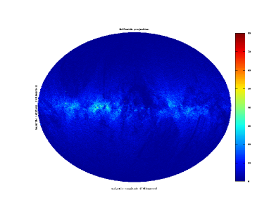
Figure 1: Mollweide projection of the sky density of all Gaia DR1 sources in Galactic coordinates.

The observational Hertzsprung-Russell (H-R) diagram in $M_{G}$ as obtained by the Gaia DR1 parallaxes versus (B-V) , evaluated as BT-VT, is presented in Figure 2 and in a contour density version in Figure 3, see also figure 1 in [16].

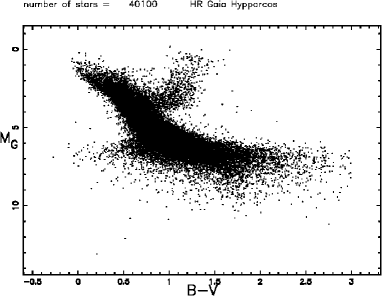
Figure 2: $M_{\mathrm{G}}$ against $(B-V)$ , evaluated as BT-VT, (H-R diagram) in the first 100 pc.

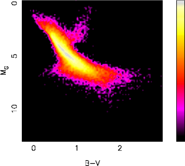
Figure 3: Contour density of stars for H-R diagram in a logarithmic scale.

The distance modulus is

$$m_{G}-M_{G}=5\,\log(d)-5\quad,$$ (2)

where $m_{g}$ is the apparent magnitude in the G-band, $M_{g}$ is the absolute magnitude in the G-band and $d$ is the distance in pc. Isolating $M_{G}$ in the above equation we obtain the theoretical curve for the upper observable absolute magnitude

$$M_{g}=-5\,\log(d)+5+m_{G}\quad,$$ (3)

once the maximum apparent magnitude in the g-band, $m_{lim}$, is inserted, i.e. $m_{G}$=12.71. Figure 4 presents the absolute magnitude as function of the distance as well the upper theoretical curve in magnitude.

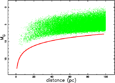
Figure 4: $M_{\mathrm{G}}$ versus distance in pc in the first 100 pc (green points) and theoretical upper curve in magnitude lower curve in the plot (red line) when $m_{G}$=12.71.

The completeness of the sample can be evaluated by the following relationship for the absolute magnitude

$$M_{g}=-{\frac{-{\it m_{lim}}\,\ln\left(10\right)+5\,\ln\left(d\right)-5\,\ln\left(10\right)}{\ln\left(10\right)}}\quad.$$ (4)

On inserting in the above formula $m_{lim}$=12.71 we obtain a numerical relationship between selected absolute magnitude and numerical relationship over which the sample is complete, see Figure 5.

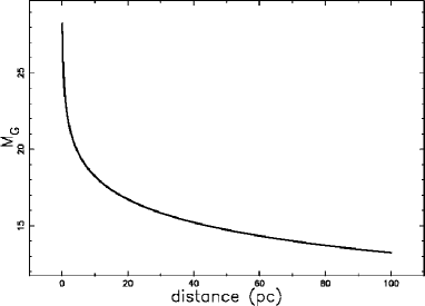
Figure 5: The relationship of completeness for $M_{\mathrm{G}}$ versus distance in pc.

In the case here considered the absolute magnitude covers the range $[3,12\,mag]$ and therefore we deal with a complete sample.

3 Standard LFs

Here we introduce an algorithm to build the LF, the statistical tests adopted, as well as the Schechter and Gamma LFs. The derived parameter for the local LF will be applied in Section 5.1 according to the general principle that the LF is equal everywhere but the upper observable absolute magnitude decreases with distance.

3.1 The astronomical LF

A LF for stars is built according to the following points

1. A standard distance is chosen, i.e. $20\,pc$,

2. The GAIA’s stars are selected according to the following ranges of existence: $-5\leq M_{V}\leq 15$ where $M_{V}$ is the absolute visual magnitude and $-0.3\leq(B-V)\leq 3$,

3. We organize an histogram with bins large 1 mag

4. We divide the obtained frequencies by the involved volume,

5. We do not apply the $1/V_{a}$ method because our sample is complete at $20\,pc$,

6. The error of the LF is evaluated as the square root of the frequencies divided by the involved volume.

The LF for Gaia’s stars is reported in Figure 6 together the LF main sequence in the V band as extracted from Table 2, column 9, in [10].

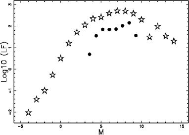
Figure 6: LF in the V band main sequence, empty stars, and Gaia’s LF, filled circles.

3.2 Statistical Tests

The merit function $\chi^{2}$ is computed as

$$\chi^{2}=\sum_{j=1}^{n}(\frac{LF_{theo}-LF_{astr}}{\sigma_{LF_{astr}}})^{2}\quad,$$ (5)

where $n$ is the number of bins for the LF of the stars and the two indices $theo$ and $astr$ stand for ‘theoretical’ and ‘astronomical’, respectively. The reduced merit function $\chi_{red}^{2}$ is evaluated by

$$\chi_{red}^{2}=\chi^{2}/NF\quad,$$ (6)

where $NF=n-k$ is the number of degrees of freedom and $k$ is the number of parameters. The goodness of the fit can be expressed by the probability $Q$, see equation 15.2.12 in [17], which involves the number of degrees of freedom and $\chi^{2}$. According to [17], the fit “may be acceptable” if $Q\geq 0.001$. The Akaike information criterion (AIC), see [18], is defined by

$$AIC=2k-2ln(L)\quad,$$ (7)

where $L$ is the likelihood function and $k$ is the number of free parameters in the model. We assume a Gaussian distribution for the errors and the likelihood function can be derived from the $\chi^{2}$ statistic $L\propto\exp(-\frac{\chi^{2}}{2})$ where $\chi^{2}$ has been computed by Equation (5), see [19], [20]. Now the AIC becomes

$$AIC=2k+\chi^{2}\quad.$$ (8)

3.3 The Schechter LF

Let $L$, the luminosity of a star, be defined in $[0,\infty]$. The Schechter LF of the stars, $\Phi$, originally applied to the stars, see [21], is

$$\Phi(L;\Phi^{*},\alpha,L^{*})dL=(\frac{\Phi^{*}}{L^{*}})(\frac{L}{L^{*}})^{\alpha}\exp\bigl{(}{-\frac{L}{L^{*}}}\bigr{)}dL\quad,$$ (9)

where $\alpha$ sets the slope for low values of $L$, $L^{*}$ is the characteristic luminosity, and $\Phi^{*}$ represents the number of stars per pc³. The normalization is

$$\int_{0}^{\infty}\Phi(L;\Phi^{*},\alpha,L^{*})dL=\rm\Phi^{*}\,\Gamma\left(\alpha+1\right)\quad,$$ (10)

where

$$\rm\Gamma\,(z)=\int_{0}^{\infty}e^{{-t}}t^{{z-1}}dt\quad,$$ (11)

is the Gamma function. The average luminosity, ${\langle L\rangle}$, is

$${\langle(\Phi(L;\Phi^{*},\alpha,L^{*})\rangle}=\rm L^{*}\,{\rm\Phi^{*}}\,\Gamma\left(\alpha+2\right)\quad.$$ (12)

An equivalent form in absolute magnitude of the Schechter LF is

$$\Phi(M;\Phi^{*},\alpha,M^{*})dM=$$

$$0.921\Phi^{*}10^{0.4(\alpha+1)(M^{*}-M)}\exp\bigl{(}{-10^{0.4(M^{*}-M)}}\bigr{)}dM\,,$$ (13)

where $M^{*}$ is the characteristic magnitude.

The resulting fitted curve is displayed in Figure 7 with parameters as in Table 1.

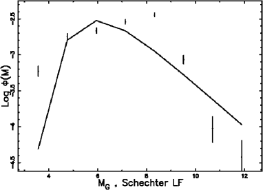
Figure 7: The observed LF for stars, empty stars with error bar, and the fit by the Schechter LF when the distance covers the range $[0\,pc,20\,pc]$.

Table 1: Parameters of the Schechter LF in the range in distance $[0\,pc,20\,pc]$ when $k=3$ and $n=8$.

$$\begin{array}[]{ccccccc}\hline\cr\hline\cr\vskip 3.0pt plus 1.0pt minus 1.0pt\cr M^{*}\,(mag)&\Psi^{*}\,(pc^{-3})&\alpha&\chi^{2}&\chi_{red}^{2}&Q&AIC\\ \vskip 3.0pt plus 1.0pt minus 1.0pt\cr\hline\cr 5.59&0.0085&-0.26&166.97&33.39&3.23\,10^{-34}&172.97\\ \hline\cr\hline\cr\end{array}$$

3.4 The Gamma LF

The Gamma LF, defined in $[0,\infty]$, is

$$f(L;\Psi^{*},L^{*},c)=\Psi^{*}\frac{\left({\frac{L}{L^{*}}}\right)^{c-1}{{\rm e}^{-{\frac{L}{L^{*}}}}}}{L^{*}\Gamma\left(c\right)}$$ (14)

where $\Psi^{*}$ is the total number of stars per pc³,

$$\mathop{\Gamma\/}\nolimits\!\left(z\right)=\int_{0}^{\infty}e^{{-t}}t^{{z-1}}dt\quad,$$ (15)

where $L^{*}\,>\,0$ is the scale and $c>\,0$ is the shape, see formula (17.23) in [22]. The average luminosity is

$$\langle f(L;\Psi^{*},L^{*},c)\rangle=\Psi^{*}L^{*}c\quad.$$ (16)

The change of parameter $(c-1)=\alpha$ allows obtaining the same scaling as for the Schechter LF (9), for more details, see [23]. The version in absolute magnitude is

$$\rm\Psi(M;\Psi^{*},c,M^{*})dM=$$

$$\frac{0.4\,{\it\Psi^{*}}\,\left({\frac{{10}^{-0.4\,M}}{{10}^{-0.4\,{M}^{{\it star}}}}}\right)^{c-1}{{\rm e}^{-{\frac{{10}^{-0.4\,M}}{{10}^{-0.4\,{M}^{{\it star}}}}}}}{10}^{-0.4\,M}\ln\left(10\right)}{{10}^{-0.4\,{M}^{{\it star}}}\Gamma\left(c\right)}dM\quad.$$ (17)

The resulting fitted curve is displayed in Figure 8 with parameters as in Table 2.

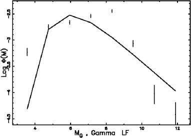
Figure 8: The observed LF for stars, empty stars with error bar, and the fit by the Gamma LF when the distance covers the range $[0\,pc,20\,pc]$.

Table 2: Parameters of the Gamma LF in the range in distance $[0\,pc,20\,pc]$ when $k=3$ and $n=8$.

$$\begin{array}[]{ccccccc}\hline\cr\hline\cr\vskip 3.0pt plus 1.0pt minus 1.0pt\cr M^{*}\,(mag)&\Psi^{*}\,(pc^{-3})&c&\chi^{2}&\chi_{red}^{2}&Q&AIC\\ \vskip 3.0pt plus 1.0pt minus 1.0pt\cr\hline\cr 5.59&0.01&0.73&166.9&33.39&3.23\,10^{-34}&172.9\\ \hline\cr\hline\cr\end{array}$$

4 Truncated LFs

Here we derive the truncated version of the Schechter and Gamma LFs.

4.1 The truncated Schechter LF

The luminosity $L$ is defined in the interval $[L_{l},L_{u}]$, where the indices $l$ and $u$ mean ‘lower’ and ‘upper’; the truncated Schechter LF, $S_{T}$, is

$$S_{T}(L;\Psi^{*},\alpha,L^{*},L_{l},L_{u})=\frac{-\left({\frac{L}{{\it L^{*}}}}\right)^{\alpha}{{\rm e}^{-{\frac{L}{{\it L^{*}}}}}}{\it\Psi^{*}}\,\Gamma\left(\alpha+1\right)}{{\it L^{*}}\,\left(\Gamma\left(\alpha+1,{\frac{L_{{u}}}{{\it L^{*}}}}\right)-\Gamma\left(\alpha+1,{\frac{L_{{l}}}{{\it L^{*}}}}\right)\right)}\quad,$$ (18)

where $\Gamma(a,z)$ is the incomplete Gamma function, defined by

$$\mathop{\Gamma\/}\nolimits\!\left(a,z\right)=\int_{z}^{\infty}t^{a-1}e^{-t}dt\quad,$$ (19)

see [24]. The average value is

$${\langle S_{T}(L;\Psi^{*},\alpha,L^{*},L_{l},L_{u})\rangle}=\frac{N}{{\it L^{*}}\left(\Gamma\left(\alpha+1,{\frac{L_{{u}}}{{\it L^{*}}}}\right)-\Gamma\left(\alpha+1,{\frac{L_{{l}}}{{\it L^{*}}}}\right)\right)}$$ (20)

with

$$N={\it\Psi^{*}}\Bigg{(}{{\it L^{*}}}^{2}\Gamma\big{(}\alpha+1,{\frac{L_{{u}}}{{\it L^{*}}}}\big{)}\alpha-{{\it L^{*}}}^{2}\Gamma\big{(}\alpha+1,{\frac{L_{{l}}}{{\it L^{*}}}}\big{)}\alpha+{{\it L^{*}}}^{2}\Gamma\big{(}\alpha+1,{\frac{L_{{u}}}{{\it L^{*}}}}\big{)}$$

$$-{{\it L^{*}}}^{2}\Gamma\big{(}\alpha+1,{\frac{L_{{l}}}{{\it L^{*}}}}\big{)}-{{\it L^{*}}}^{-\alpha+1}{{\rm e}^{-{\frac{L_{{l}}}{{\it L^{*}}}}}}{L_{{l}}}^{\alpha+1}+{{\it L^{*}}}^{-\alpha+1}{{\rm e}^{-{\frac{L_{{u}}}{{\it L^{*}}}}}}{L_{{u}}}^{\alpha+1}\Bigg{)}\times$$

$$\Gamma\big{(}\alpha+1\big{)}\quad.$$ (21)

The four luminosities $L,L_{l},L^{*}$ and $L_{u}$ are connected with the absolute magnitudes $M$, $M_{l}$, $M_{u}$ and $M^{*}$ through the following relation,

$$\frac{L}{L_{\hbox{$\odot$}}}=10^{0.4(M_{\hbox{$\odot$}}-M)}\quad,\frac{L_{l}}{L_{\hbox{$\odot$}}}=10^{0.4(M_{\hbox{$\odot$}}-M_{u})}\quad,$$

$$\frac{L^{*}}{L_{\hbox{$\odot$}}}=10^{0.4(M_{\hbox{$\odot$}}-M^{*})}\,\quad,\frac{L_{u}}{L_{\hbox{$\odot$}}}=10^{0.4(M_{\hbox{$\odot$}}-M_{l})}$$ (22)

where the indices $u$ and $l$ are inverted in the transformation from luminosity to absolute magnitude and $L_{\hbox{$\odot$}}$ and $M_{\hbox{$\odot$}}$ are the luminosity and absolute magnitude of the sun in the considered band. The equivalent form in absolute magnitude of the truncated Schechter LF is therefore

$$\Psi(M;\Psi^{*},\alpha,M^{*},M_{l},M_{u})dM=\frac{AS}{DS}\quad,$$ (23)

with

$$AS=-0.4\left({10}^{0.4{\it M^{*}}-0.4M}\right)^{\alpha}{{\rm e}^{-{10}^{0.4{\it M^{*}}-0.4M}}}\times$$

$${\it\Psi^{*}}\Gamma\left(\alpha+1\right){10}^{0.4{\it M^{*}}-0.4M}\left(\ln\left(2\right)+\ln\left(5\right)\right)$$ (24)

and

$$DS=\Gamma\left(\alpha+1,{10}^{-0.4M_{{l}}+0.4{\it M^{*}}}\right)-\Gamma\left(\alpha+1,{10}^{0.4{\it M^{*}}-0.4M_{{u}}}\right)$$ (25)

The averaged absolute magnitude, $\langle M\rangle$, is

$${\langle\Psi(M;\Psi^{*},\alpha,M^{*},M_{l},M_{u})\rangle}=$$

$$\frac{\int_{M_{l}}^{M_{u}}M(M;\Psi^{*},\alpha,L^{*},L_{l},L_{u})MdM}{\int_{M_{l}}^{M_{u}}M(M;\Psi^{*},\alpha,L^{*},L_{l},L_{u})dM}\quad.$$ (26)

More details can be found in [25].

The resulting fitted curve is displayed in Figure 9 with parameters as in Table 3.

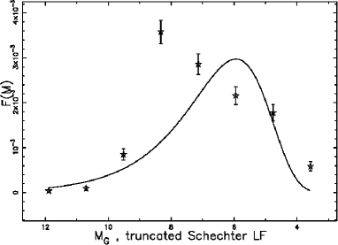
Figure 9: The observed LF for stars, empty stars with error bar, and the fit by the truncated Schechter LF when the distance covers the range $[0\,pc,20\,pc]$.

Table 3: Parameters of the truncated Schechter LF in the range in distance $[0\,pc,20\,pc]$ when $k=5$ and $n=8$.

$$\begin{array}[]{ccccccccc}\hline\cr\hline\cr\vskip 3.0pt plus 1.0pt minus 1.0pt\cr M^{*}&M_{l}&M_{u}&\Psi^{*}&\alpha&\chi^{2}&\chi_{red}^{2}&Q&AIC\\ \vskip 3.0pt plus 1.0pt minus 1.0pt\cr\hline\cr 5.6&3.56&11.89&0.0083&-0.26&167&55.67&5.54\,10^{-36}&177\\ \hline\cr\hline\cr\end{array}$$

4.2 The truncated Gamma LF

The truncated Gamma LF is defined in the interval $[L_{l},L_{u}]$

$$f(L;\Psi^{*},L^{*},c,L_{l},L_{u})=\Psi^{*}\,k\;\left({\frac{L}{{\it L^{*}}}}\right)^{c-1}{{\rm e}^{-{\frac{L}{{\it L^{*}}}}}}$$ (27)

where the constant $k$ is

$$k=$$

$$\frac{c}{{\it L^{*}}\,\left(\left({\frac{L_{{u}}}{{\it L^{*}}}}\right)^{c}{{\rm e}^{-{\frac{L_{{u}}}{{\it L^{*}}}}}}-\Gamma\left(1+c,{\frac{L_{{u}}}{{\it L^{*}}}}\right)+\Gamma\left(1+c,{\frac{L_{{l}}}{{\it L^{*}}}}\right)-\left({\frac{L_{{l}}}{{\it L^{*}}}}\right)^{c}{{\rm e}^{-{\frac{L_{{l}}}{{\it L^{*}}}}}}\right)}\,.$$ (28)

Its expected value is

$$\langle f(L;\Psi^{*},L^{*},c,L_{l},L_{u})\rangle=$$

$$\Psi^{*}\frac{-c\left(\Gamma\left(1+c,{\frac{L_{{u}}}{{\it L^{*}}}}\right)-\Gamma\left(1+c,{\frac{L_{{l}}}{{\it L^{*}}}}\right)\right){\it L^{*}}}{\left({\frac{L_{{u}}}{{\it L^{*}}}}\right)^{c}{{\rm e}^{-{\frac{L_{{u}}}{{\it L^{*}}}}}}-\Gamma\left(1+c,{\frac{L_{{u}}}{{\it L^{*}}}}\right)+\Gamma\left(1+c,{\frac{L_{{l}}}{{\it L^{*}}}}\right)-\left({\frac{L_{{l}}}{{\it L^{*}}}}\right)^{c}{{\rm e}^{-{\frac{L_{{l}}}{{\it L^{*}}}}}}}\quad.$$ (29)

More details on the truncated Gamma PDF can be found in [26, 27, 23]. The Gamma truncated LF in magnitude is

$$\Psi(M;\Psi^{*},c,M^{*},M_{l},M_{u})dM=$$

$$\frac{0.4\,c\left({10}^{0.4\,{\it M^{*}}-0.4\,M}\right)^{c}{{\rm e}^{-{10}^{0.4\,{\it M^{*}}-0.4\,M}}}{\it\Psi^{*}}\,\left(\ln\left(2\right)+\ln\left(5\right)\right)}{D}$$ (30)

where

$$D=$$

$${{\rm e}^{-{10}^{-0.4\,M_{{l}}+0.4\,{\it M^{*}}}}}\left({10}^{-0.4\,M_{{l}}+0.4\,{\it M^{*}}}\right)^{c}$$

$$-{{\rm e}^{-{10}^{0.4\,{\it M^{*}}-0.4\,M_{{u}}}}}\left({10}^{0.4\,{\it M^{*}}-0.4\,M_{{u}}}\right)^{c}$$

$$-\Gamma\left(1+c,{10}^{-0.4\,M_{{l}}+0.4\,{\it M^{*}}}\right)+\Gamma\left(1+c,{10}^{0.4\,{\it M^{*}}-0.4\,M_{{u}}}\right)\quad.$$ (31)

The averaged absolute magnitude, $\langle M\rangle$, is defined numerically as in Equation 26.

The resulting fitted curve is displayed in Figure 10 with parameters as in Table 4.

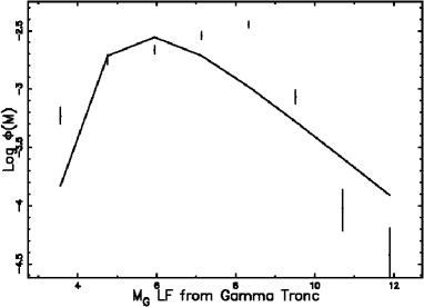
Figure 10: The observed LF for stars, empty stars with error bar, and the fit by the truncated Gamma LF when the distance covers the range $[0\,pc,20\,pc]$.

Table 4: Parameters of the truncated Gamma LF in the range in distance $[0\,pc,20\,pc]$ when $k=5$ and $n=8$.

$$\begin{array}[]{ccccccccc}\hline\cr\hline\cr\vskip 3.0pt plus 1.0pt minus 1.0pt\cr M^{*}&M_{l}&M_{u}&\Psi^{*}&c&\chi^{2}&\chi_{red}^{2}&Q&AIC\\ \vskip 3.0pt plus 1.0pt minus 1.0pt\cr\hline\cr 5.3&3.56&11.89&0.01&0.67&169&56.33&2.02\,10^{-36}&179\\ \hline\cr\hline\cr\end{array}$$

5 Distance effects

We model the average absolute magnitude of the stars as a function of the distance, the photometric maximum in the number of stars for a given flux as a function of the distance, and the average distance of the stars for a given flux in the framework of the two truncated LFs here considered.

5.1 Averaged absolute magnitude

In order to model the influence of the distance $d$ in pc on the LF, an empirical variable lower bound in absolute magnitude, $M_{l}$, has been introduced,

$$M_{l}(d)=5.53-0.27\,d^{0.7}\quad.$$ (32)

The upper bound, $M_{u}$ was already fixed by the nonlinear equation (3). A second distance correction is

$$M^{*}=M_{u}(d)-2.8-5.2\exp{-\frac{d}{100}}\quad,$$ (33)

where $M_{u}(d)$ has been defined in Equation (3). Figure 11 compares the theoretical average absolute magnitudes for the truncated Schechter LF with the observed ones; the value of $M^{*}$ in Equation (33) minimizes the difference between the two curves.

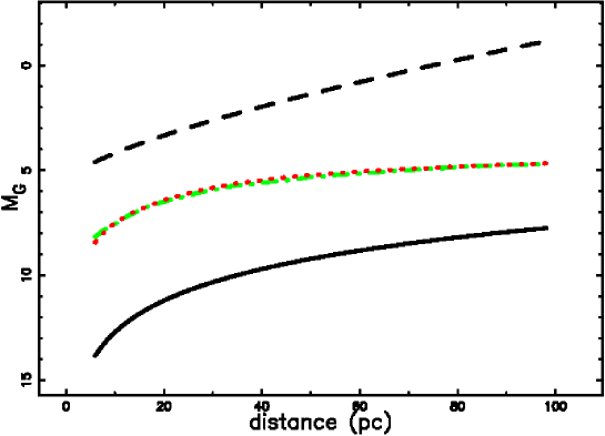
Figure 11: Average observed absolute G-magnitude versus distance for Gaia (green points), average theoretical absolute magnitude for truncated Schechter LF with $\alpha=-0.61$ as given by Equation (26) (dot-dash-dot red line), curve for the empirical lowest absolute magnitude at a given distance, see Equation (32) (full black line) and the theoretical curve for the highest absolute magnitude at a given distance (dashed black line), see Equation (3).

Conversely Figure 12 compares the theoretical average absolute magnitudes for the truncated Gamma LF with the observed ones; also here the value of $M^{*}$ obtained from Equation (33) minimizes the difference between the two curves.

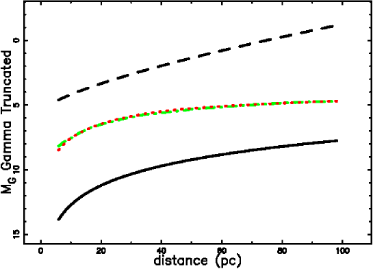
Figure 12: Average observed absolute G-magnitude versus distance for Gaia (green points), average theoretical absolute magnitude for truncated Gamma LF with $c=0.38$ as given by the analogue of equation (26) (dot-dash-dot red line), theoretical curve for the empirical lowest absolute magnitude at a given distance, see Equation (32) (full black line) and the theoretical curve for the highest absolute magnitude at a given distance (dashed black line), see Equation (3).

5.2 The photometric maximum

The definition of the flux, $f$, is

$$f=\frac{L}{4\pi r^{2}}\quad,$$ (34)

where $r$ is the distance and $L$ the luminosity of the star. The joint distribution in distance, r, and flux, f, for the number of stars is

$$\frac{dN}{d\Omega drdf}=\frac{1}{4\,\pi}\int_{0}^{\infty}4\pi r^{2}dr\Phi(\frac{L}{L^{*}})\delta(f-\frac{L}{4\,\pi\,r^{2}})\quad,$$ (35)

were the factor ($\frac{1}{4\pi}$) converts the number density into density for solid angle and the Dirac delta function selects the required flux. We now apply the sifting properties of the delta function, see [28], to the case of the Schechter LF as given by formula 9

$$\frac{dN}{d\Omega drdf}=\frac{1}{L^{*}}\,4\,\pi\,{r}^{4}{\it\Phi^{*}}\,\left(4\,{\frac{\pi\,f{r}^{2}}{{\it L^{*}}}}\right)^{\alpha}{{\rm e}^{-4\,{\frac{\pi\,f{r}^{2}}{{\it L^{*}}}}}}\quad.$$ (36)

We now introduce the critical radius $r_{crit}$

$$r_{crit}=\frac{1}{2}\,{\frac{\sqrt{{\it L^{*}}}}{\sqrt{\pi}\sqrt{f}}}\quad.$$ (37)

Therefore the joint distribution in distance and flux becomes

$$\frac{dN}{d\Omega drdf}=\frac{1}{L^{*}}\,4\,\pi\,{r}^{4}{\it\Phi^{*}}\,\left({\frac{{r}^{2}}{{{\it r_{crit}}}^{2}}}\right)^{\alpha}{{\rm e}^{-{\frac{{r}^{2}}{{{\it r_{crit}}}^{2}}}}}\quad.$$ (38)

The above number of stars has a maximum at $r=r_{max}$:

$$r_{max}=\sqrt{2+\alpha}{\it r_{crit}}\quad,$$ (39)

and the average distance of the stars, ${\langle r\rangle}$, is

$$\langle r\rangle={\frac{{\it r_{crit}}\,\Gamma\left(3+\alpha\right)}{\Gamma\left(\frac{5}{2}+\alpha\right)}}\quad.$$ (40)

Figure 13 presents the number of stars observed in Gaia as a function of the distance for a given window in the flux, as well as the theoretical curve.

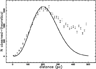
Figure 13: The stars of Gaia with $1243361.38\,(e-/s)\leq f\leq 1450291.3\,(e-/s)$ or $10.121\,(mag)\leq G\,(mag)\,\leq 10.288$ are organized by frequency versus distance, (empty circles); the error bar is given by the square root of the frequency. The maximum frequency of the observed stars is at $d=247$ pc. The full line is the theoretical curve generated by $\frac{dN}{d\Omega drdf}$ as given by the application of the Schechter LF which is Equation (36) and the theoretical maximum is at $d=274$ pc. The parameters are $L^{*}=5\,10^{11}$ (e-/s)$\times$ pc² and $\alpha$ =-0.62. Case of the Schechter LF.

Figure 14 presents the observed position of the maximum of the number of stars as a function of the flux.

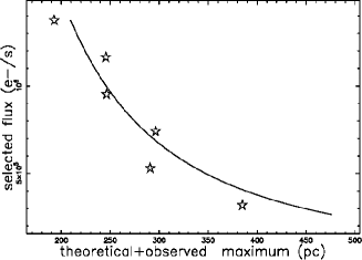
Figure 14: Position of the observed maximum as function of the flux (empty stars) and theoretical average value as given by Equation (40) for the Schechter LF (full line). The parameters are $L^{*}=5.5\,10^{11}$ (e-/s)$\times$ pc² and $\alpha$ =-0.62. Case of the Schechter LF.

In order to shift to more familiar variables Figure 15 reports the position of the above maximum as function of the apparent Gaia magnitude

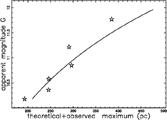
Figure 15: Position of the observed maximum as function of the apparent magnitude, G, (empty stars) and theoretical average value as given by Equation (40) for the Schechter LF (full line). The parameters are the same of Figure 14. Case of the Schechter LF.

Figures 16 and 17 present the observed average value of the number of stars as a function of the flux and apparent magnitude.

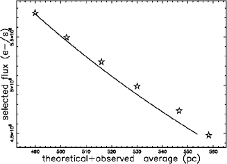
Figure 16: Position of the average distance of the stars as function of the flux (empty stars) and theoretical curve as given by Equation (39) (full line) for the Schechter LF. The parameters are $L^{*}=1.3\,10^{13}$ (e-/s)$\times$ pc² and $\alpha$ =-0.62. Case of the Schechter LF.

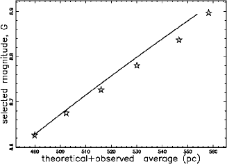
Figure 17: Position of the average distance of the stars as function of the apparent magnitude, G, (empty stars) and theoretical curve as given by Equation (39) (full line) for the Schechter LF. The parameters are the same of Figure 16. Case of the Schechter LF.

In the case of the Gamma LF, the maximum in the number of stars is at

$$r_{max}=\sqrt{c+1}{r_{crit}}\quad,$$ (41)

and the average distance of the stars ${\langle r\rangle}$, is

$$\langle r\rangle={\frac{{r_{crit}}\,c\left(c+1\right)\Gamma\left(c\right)}{\Gamma\left(\frac{3}{2}+c\right)}}\quad.$$ (42)

6 Conclusions

Standard LFs. The Schechter function and the Gamma PDF can model the LF for stars, see Tables 1 and 2 as well as Figures 7 and 8, but the values of the involved parameters depend on the chosen distance.
Truncated LFs. The truncated Schechter function and the truncated Gamma LF can model the averaged absolute magnitude as a function of the distance, see Figures 11 and 12. As an example, four analytical equations have been used in the case of the truncated Schechter LF: (i) the average theoretical absolute magnitude for the truncated Schechter LF, see Equation (26), (ii) an empirical expression for the lowest absolute magnitude at a given distance, see Equation (32), (iii) a theoretical curve for the highest absolute magnitude at a given distance, see Equation (3), and (iv) a distance dependence expression for $M^{*}$ as given by Equation 33. The above four equations model the Malmquist bias.
Photometric maximum The number of stars as a function of the distance presents a maximum which is a function of the flux, see Figures 13 and 14 for the Schechter LF. The theoretical and observed average distance of the stars are also functions of the selected flux, see Figure 16.
Topics not covered The treatment here adopted deals with an homogeneous distribution of stars and therefore the the vertical scale-heights are not covered, see [10].

Bibliography

Bibliography

- [1] Malmquist K G 1920 A study of the stars of spectral type A Lund Medd. Ser. II 22, 1
- [2] Malmquist K G 1922 On some relations in stellar statistics Lund Medd. Ser. I 100, 1
- [3] Malmquist K G 1936 Investigations on the stars in high galactic latitudes II. Photographic magnitudes and colour indices of about 4500 stars near the north galactic pole. Stockholms Observatoriums Annaler 12, 7.1
- [4] Binney J and Merrifield M 1998 Galactic astronomy (Princeton, NJ: Princeton University Press)
- [5] Butkevich A G, Berdyugin A V and Teerikorpi P 2005 Statistical biases in stellar astronomy: the Malmquist bias revisited MNRAS 362, 321
- [6] Eddington A S 1914 Stellar movements and the structure of the universe (London: Macmillan and co.)
- [7] Jaschek C and Gomez A E 1985 The Malmquist correction A&A 146, 387
- [8] Wielen R 1974 The kinematics and ages of stars in Gliese’s catalogue Highlights of Astronomy 3, 395
- [9] Flynn C, Holmberg J, Portinari L, Fuchs B and Jahreiß H 2006 On the mass-to-light ratio of the local Galactic disc and the optical luminosity of the Galaxy MNRAS 372, 1149 (Preprint astro-ph/0608193)
- [10] Just A, Fuchs B, Jahreiß H, Flynn C, Dettbarn C and Rybizki J 2015 The local stellar luminosity function and mass-to-light ratio in the near-infrared MNRAS 451, 149 (Preprint 1504.05808)
- [11] Gaia Collaboration, Prusti T, de Bruijne J H J, Brown A G A, Vallenari A, Babusiaux C, Bailer-Jones C A L, Bastian U, Biermann M, Evans D W and et al 2016 The Gaia mission A&A 595 A1 (Preprint 1609.04153)
- [12] Gaia Collaboration, Brown A G A, Vallenari A, Prusti T, de Bruijne J H J, Mignard F, Drimmel R, Babusiaux C, Bailer-Jones C A L, Bastian U and et al 2016 Gaia Data Release 1. Summary of the astrometric, photometric, and survey properties A&A 595 A2 (Preprint 1609.04172)
- [13] Stassun K G and Torres G 2016 Evidence for a Systematic Offset of -0.25 mas in the Gaia DR1 Parallaxes ApJ 831 L6
- [14] Evans D W, Riello M, De Angeli F, Busso G, van Leeuwen F, Jordi C, Fabricius C, Brown A G A, Carrasco J M, Voss H and et al 2017 Gaia Data Release 1. Validation of the photometry A&A 600 A51 (Preprint 1701.05873)
- [15] Carrasco J M, Evans D W, Montegriffo P, Jordi C, van Leeuwen F, Riello M, Voss H, De Angeli F, Busso G and et al 2016 Gaia Data Release 1. Principles of the photometric calibration of the G band A&A 595 A7 (Preprint 1611.02036)
- [16] van Leeuwen F, Evans D W, De Angeli F, Jordi C, Busso G, Cacciari C, Riello M, Pancino E, Altavilla G and et al 2017 Gaia Data Release 1. The photometric data A&A 599 A32 (Preprint 1612.02952)
- [17] Press W H, Teukolsky S A, Vetterling W T and Flannery B P 1992 Numerical Recipes in FORTRAN. The Art of Scientific Computing (Cambridge, UK: Cambridge University Press)
- [18] Akaike H 1974 A new look at the statistical model identification IEEE Transactions on Automatic Control 19, 716
- [19] Liddle A R 2004 How many cosmological parameters? MNRAS 351, L49
- [20] Godlowski W and Szydowski M 2005 Constraints on Dark Energy Models from Supernovae in M Turatto, S Benetti, L Zampieri and W Shea, eds, 1604-2004: Supernovae as Cosmological Lighthouses vol 342 of Astronomical Society of the Pacific Conference Series pp 508–516
- [21] Schechter P 1976 An analytic expression for the luminosity function for galaxies. ApJ 203, 297
- [22] Johnson N L, Kotz S and Balakrishnan N 1994 Continuous univariate distributions. Vol. 1. 2nd ed. (New York: Wiley )
- [23] Zaninetti L 2016 Pade approximant and minimax rational approximation in standard cosmology Galaxies 4(1), 4 ISSN 2075-4434 URL http://www.mdpi.com/2075-4434/4/1/4
- [24] Olver F W J e, Lozier D W e, Boisvert R F e and Clark C W e 2010 NIST handbook of mathematical functions. (Cambridge: Cambridge University Press. )
- [25] Zaninetti L 2017 A left and right truncated schechter luminosity function for quasars Galaxies 5(2), 25
- [26] Zaninetti L 2013 A right and left truncated gamma distribution with application to the stars Advanced Studies in Theoretical Physics 23, 1139
- [27] Okasha M K and Alqanoo I M 2014 Inference on The Doubly Truncated Gamma Distribution For Lifetime Data International Journal Of Mathematics And Statistics Invention 2, 1
- [28] Bracewell R N 2000 The Fourier transform and its applications (New York: McGraw-Hill)