ADE surfaces and their moduli

Abstract.

We define a class of surfaces corresponding to the $ADE$ root lattices and construct compactifications of their moduli spaces as quotients of projective varieties for Coxeter fans, generalizing Losev-Manin spaces of curves. We exhibit modular families over these moduli spaces, which extend to families of stable pairs over the compactifications. One simple application is a geometric compactification of the moduli of rational elliptic surfaces that is a finite quotient of a projective toric variety.

1. Introduction

There are two sources of motivation for this work: Losev-Manin spaces [LM00] and degenerations of K3 surfaces with a nonsymplectic involution [AET19].

Let $L_{n+3}$ be the moduli space parameterizing weighted stable curves $(Z,Q_{0}+Q_{\infty}+\epsilon\sum_{i=1}^{n+1}P_{i})$ of genus 0 with $n+3$ points, where $0<\epsilon\ll 1$. Equivalently, the singularity condition is that the $n+1$ points $P_{i}$ are allowed to collide while the remaining two may not collide with any others. One has $\dim L_{n+3}=n$. Quite remarkably, $L_{n+3}$ is a projective toric variety for the Coxeter fan (also called the Weyl chamber fan) for the root lattice $A_{n}$, formed by the mirrors to the roots. Of course it comes with an action of the Weyl group $W(A_{n})=S_{n+1}$ permuting the points $P_{i}$. The moduli space of the pairs $(Z,Q_{0}+Q_{\infty}+\epsilon R)$ for the divisor $R=\sum_{i=1}^{n+1}P_{i}$ with unordered points is then $L_{n+3}/S_{n+1}$.

There are other ways in which $L_{n+3}$ corresponds to the root lattice $A_{n}$. For example, its interior, over which the fibers are $Z\simeq{\mathbb{P}}^{1}$, is the torus $\operatorname{Hom}(A_{n},{\mathbb{C}}^{*})$, and the discriminant locus, where some of the points $P_{i},P_{j}$ coincide, is a union of root hypertori $\cup_{\alpha}\{e^{\alpha}=1\}$ with $\alpha=e_{i}-e_{j}$ going over the roots of $A_{n}$. Additionally, the worst singularity that the divisor $\sum P_{i}$ can have is $(x-1)^{n+1}=0$, which is an $A_{n}$-singularity.

Losev and Manin asked in [LM00] if similar moduli spaces existed for other root lattices. This was partially answered by Batyrev and Blume in [BB11] where they constructed compact moduli spaces for the $B_{n}$ and $C_{n}$ lattices as moduli of certain pointed rational curves with an involution. Batyrev-Blume’s method works only for infinite series of root lattices, such as $ABCD$, and it breaks down for $D_{n}$ where it leads to non-flat families (most fibers have dimension 1 but some have 2).

In this paper, we generalize Losev-Manin spaces to the $D_{n}$ and $E_{n}$ lattices by replacing stable curve pairs $(Z,Q_{0}+Q_{\infty}+\epsilon R)$ by (KSBA) stable slc surface pairs $(X,D+\epsilon R)$ and constructing their compact moduli.

Namely, we define a class of surface pairs $(X,D+\epsilon R)$ naturally associated with the root lattices $A_{n}$, $D_{n}$, and $E_{n}$. We call these pairs $ADE$ double covers, as all of them are double covers $\pi\colon X\to Y$ of surface pairs $(Y,C+\frac{1+\epsilon}{2}B)$ . Here, $C$ and $D$ are reduced boundaries (downstairs and upstairs), $R$ is the ramification divisor, and $B$ is the branch divisor of $\pi$. We call the pairs $(Y,C+\frac{1+\epsilon}{2}B)$ the $ADE$ pairs, and the underlying pairs $(Y,C)$ the $ADE$ surfaces (with reduced boundary $C$).

We prove that the moduli space $M$ of $ADE$ pairs (equivalently of $ADE$ double covers) of a fixed type is a torus for the associated $ADE$ lattice $\Lambda$ modulo a Weyl group $W$, and that the normalization of the moduli compactification ${\overline{M}}^{\rm slc}$ is the $W$-quotient of a projective toric variety for a generalized Coxeter fan corresponding to $\Lambda$. Moreover, for each type we construct an explicit modular family of $ADE$ pairs over $M$ and show that, after a suitable coordinate change, the discriminant locus in $M$, where $B$ is singular, is a union of root hypertori $\cup_{\alpha}\{e^{\alpha}=1\}$ with $\alpha$ going over the roots of $\Lambda$. Additionally, the worst singularity appearing in the double cover $X$ is the surface Du Val singularity of type $\Lambda$.

For $\Lambda=A_{n}$ we get the standard Coxeter fan and ${\overline{M}}^{\rm slc}=L_{n+3}/S_{n+1}$. The ramification curve $R=B$ in this case is hyperelliptic, a double cover $f\colon B\to Z$ of a rational genus 0 curve. The boundary $C$ has two irreducible components defining the boundary $Q_{0}+Q_{\infty}$ of $Z$, and the ramification points of $f$ provide the remaining $n+1$ points in the data for a stable Losev-Manin curve $(Z,Q_{0}+Q_{\infty}+\epsilon\sum_{i=1}^{n+1}P_{i})$.

For $\Lambda=D_{n}$ and $E_{n}$ the fan is a generalized Coxeter fan, a coarsening of the standard Coxeter fan. It is the normal fan of a permutahedron given by a classical Wythoff construction.

We found these $ADE$ surfaces and pairs by studying degenerations of K3 surfaces of degree 2. A polarized K3 surface $(X,L)$ of degree $L^{2}=2$ comes with a canonical double cover $\pi\colon X\to Y$. The ramification divisor $R$ of $\pi$ is intrinsic to $(X,L)$, and the pair $(X,\epsilon R)$ is a stable slc pair. Thus, the moduli of (KSBA) stable slc pairs provides a canonical moduli compactification ${\overline{F}}_{2}^{\rm slc}$ of the moduli space $F_{2}$ of K3 surfaces of degree 2.

On the other hand, there exists a nice toroidal compactification ${\overline{F}}_{2}^{\rm tor}$ defined by the Coxeter fan for the reflection group of the root lattice associated to $F_{2}$. The type III strata of ${\overline{F}}_{2}^{\rm tor}$ are products of $W$-quotients of projective toric varieties for the Coxeter fans of certain $ADE$ root lattices. These strata look like the moduli spaces of degenerate stable slc pairs $(Y,C+\frac{1+\epsilon}{2}B)$ whose irreducible components $(Y_{i},C_{i}+\frac{1+\epsilon}{2}B_{i})$ are some of the $ADE$ surface pairs discussed above. Indeed, we confirmed this in many examples. We determine the precise connection between ${\overline{F}}_{2}^{\rm slc}$ and ${\overline{F}}_{2}^{\rm tor}$ in [AET19], which is a continuation of this paper.

We work over the field ${\mathbb{C}}$ of complex numbers. Throughout, $\epsilon$ will denote a sufficiently small real number: $0<\epsilon\ll 1$. This means that for fixed numerical invariants there exists an $\epsilon_{0}>0$ such that the stated conditions hold for any $0<\epsilon\leq\epsilon_{0}$. Now let us explain the main results and the structure of the present paper in more detail.

In Section 2 we define $(K+D)$-trivial polarized involution pairs $(X,D,\iota)$ and study their basic properties. Roughly speaking, such pairs consist of a normal surface $X$ with an anticanonical divisor $D$ and an involution $\iota\colon X\to X$ that preserves $D$. They naturally appear when studying stable degenerations of K3 surfaces with a nonsymplectic involution. We prove that the quotient $(Y,C)=(X,D)/\iota$ of an involution pair is a log del Pezzo surface of index 2, i.e. the divisor $-2(K_{Y}+C)$ is Cartier and ample.

Denoting by $\pi\colon X\to Y$ the double cover, $B\in|-2(K_{Y}+C)|$ the branch divisor and $R\subset X$ the ramification divisor, one has $K_{X}+D+\epsilon R=\pi^{*}(K_{Y}+C+\frac{1+\epsilon}{2}B)$. Then the pair $(X,D+\epsilon R)$ is a (KSBA) stable slc pair iff the pair $(Y,C+\frac{1+\epsilon}{2}B)$ is such.

By analogy with Kulikov degenerations of K3 surfaces, we divide the pairs $(X,D,\iota)$ and their quotients $(Y,C)$ into types I, II, III. For type I, one has $C=D=0$, the surface $X$ is an ordinary K3 surface with Du Val singularities, and the pair $(Y,C+\frac{1+\epsilon}{2}B)$ is klt. For types II and III, the pairs $(X,D+\epsilon R)$ and $(Y,C+\frac{1+\epsilon}{2}B)$ are both not klt; these types are distinguished by the properties of the boundary $D$, which is a disjoint union of smooth elliptic curves in type II and a cycle of rational curves in type III.

With this motivation, we set out to investigate log canonical non-klt del Pezzo surfaces with boundary $(Y,C)$ of index 2, and the moduli spaces of log canonical pairs $(Y,C+\frac{1+\epsilon}{2}B)$, with $B\in|-2(K_{Y}+C)|$.

In Section 3 we explicitly define many examples of such surfaces $(Y,C)$ in an ad hoc way. Since the word type is already used for “types I, II, III”, we call the combinatorial classes of such surfaces shapes. Those of type III we call $ADE$ shapes, and of type II we call ${\widetilde{A}}{\widetilde{D}}{\widetilde{E}}$ shapes. We call the corresponding surfaces $(Y,C)$ $ADE$ resp. ${\widetilde{A}}{\widetilde{D}}{\widetilde{E}}$ surfaces, the stable pairs $(Y,C+\frac{1+\epsilon}{2}B)$ $ADE$ resp. ${\widetilde{A}}{\widetilde{D}}{\widetilde{E}}$ pairs, and their covers $(X,D+\epsilon R)$ $ADE$ resp. ${\widetilde{A}}{\widetilde{D}}{\widetilde{E}}$ double covers. To each shape we associate a decorated $ADE$, resp. ${\widetilde{A}}{\widetilde{D}}{\widetilde{E}}$ Dynkin diagram, which we use to label the shape, and a corresponding $ADE$, resp. ${\widetilde{A}}{\widetilde{D}}{\widetilde{E}}$ lattice. The main reason for this association comes later, when considering the moduli spaces and their compactifications.

In the simplest cases, the surfaces $Y$ are toric and $C$ is a part of the toric boundary, with two components $C_{1},C_{2}$ in type III and one component in type II. These shapes are labeled by diagrams of types $A_{n}$, $D_{n}$, $E_{n}$, ${\widetilde{D}}_{2n}$, ${\widetilde{E}}_{7}$ and ${\widetilde{E}}_{8}$. At this point there is a clear motivation behind this labeling scheme, as the defining lattice polytopes of the toric surfaces $Y$ contain the corresponding Dynkin diagrams in an obvious way. In type II we also introduce several nontoric shapes, which we call ${\widetilde{A}}_{2n-1}$, ${\widetilde{A}}_{1}^{*}$, and ${\widetilde{A}}_{0}^{-}$. Interestingly there is no ${\widetilde{E}}_{6}$ shape; Remark 3.10 discusses some reasons for that.

Next we define a procedure, which we call priming, for producing a new lc nonklt del Pezzo pair $({\overline{Y}}^{\prime},{\overline{C}}^{\prime})$ of index 2 from an old such pair $(Y,C)$. The procedure consists of making weighted blowups $Y^{\prime}\to Y$ at a collection of up to 4 points on the boundary $C$, and then performing a contraction $Y^{\prime}\to{\overline{Y}}^{\prime}$ defined by the divisor $-2(K_{Y^{\prime}}+C^{\prime})$ (where $C^{\prime}$ is the strict transform of $C$), provided that it is big and nef.

We list all the $ADE$ and ${\widetilde{A}}{\widetilde{D}}{\widetilde{E}}$ shapes, together with their basic numerical invariants and singularities in Tables 2 and 3. In all, there are 43 $ADE$ shapes and 17 ${\widetilde{A}}{\widetilde{D}}{\widetilde{E}}$ shapes, some of which define infinite families. Whilst this list seems rather large, most are obtained by applying the priming operation to a very short list of fundamental shapes. We call these fundamental shapes pure shapes, and call the ones obtained from them by priming primed shapes.

In Section 4 we prove our first main result, which justifies our interest in the $ADE$ and ${\widetilde{A}}{\widetilde{D}}{\widetilde{E}}$ surfaces.

Theorem A.

The log canonical non-klt del Pezzo surfaces $(Y,C)$ with $2(K_{X}+C)$ Cartier and $C$ reduced (or possibly empty) are exactly the same as the $ADE$ and ${\widetilde{A}}{\widetilde{D}}{\widetilde{E}}$ surfaces $(Y,C)$, pure and primed.

Most of the proof can be extracted from the work of Nakayama [Nak07], with additional arguments necessary in genus 1. Nakayama’s classification of log del Pezzo pairs of index 2 was done in very different terms and the connection with root lattices did not appear in it.

In Section 5, for each shape we describe the moduli spaces of $ADE$ (i.e. type III) pairs and their double covers. For each shape we have a root lattice $\Lambda$ of $ADE$ type. It has an associated torus $T_{\Lambda}:=\operatorname{Hom}(\Lambda,{\mathbb{C}}^{*})$ and Weyl group $W_{\Lambda}$. Then our second main result is as follows.

Theorem B.

The moduli stack of $ADE$ pairs of a fixed $ADE$ shape is

$$[\operatorname{Hom}(\Lambda^{*},{\mathbb{C}}):\mu_{\Lambda}\times\mu_{2}]=[T_{\Lambda}:W_{\Lambda}\times\mu_{2}] A$$ for pure shapes,

$$[\operatorname{Hom}(\Lambda^{*},{\mathbb{C}}):\mu_{\Lambda}]=[T_{\Lambda}:W_{\Lambda}] D E$$ for pure and shapes,

$$[\operatorname{Hom}(\Lambda^{*},{\mathbb{C}}):\mu_{\Lambda^{\prime}}\times W_{0}]=[T_{\Lambda^{\prime}}:W_{\Lambda}\rtimes W_{0}]$$ for primed shapes.

Here, $\Lambda$ is an $ADE$ root lattice, $\Lambda^{*}$ is its dual weight lattice, $\Lambda^{\prime}$ is a lattice satisfying $\Lambda\subset\Lambda^{\prime}\subset\Lambda^{*}$ given explicitly in Theorem 5.12, $T_{\Lambda^{\prime}}:=\operatorname{Hom}(\Lambda^{\prime},{\mathbb{C}}^{*})$, $\mu_{\Lambda^{\prime}}:=\operatorname{Hom}(\Lambda^{*}/\Lambda^{\prime},{\mathbb{C}}^{*})$, and the additional Weyl group $W_{0}$ is given in Theorem 3.32, with action described in Theorem 5.13.

This result is proved as Thms. 5.9 (for pure shapes) and 5.12 (for primed shapes). To conclude Section 5, for each pure $ADE$ shape we construct a Weyl group invariant modular family of $ADE$ pairs, which we call the naive family, over the torus $T_{\Lambda^{*}}$.

In Section 6 for each $ADE$ (i.e. type III) shape we construct a modular compactification of the moduli space of $ADE$ pairs of this shape. In  6A we begin with a general discussion of moduli compactifications using stable pairs, and we define stable $ADE$ pairs. Next, for each $ADE$ shape we construct a Weyl group invariant family of stable slc pairs $(Y,C+\frac{1+\epsilon}{2}B)$ over a projective toric variety $V_{M}^{\rm cox}$ for the Coxeter fan of an appropriate over-lattice $M\supset\Lambda^{*}$ of index $2^{k}$ (Thms. 6.18, 6.26, 6.28). These theorems also describe the combinatorial types of the stable pairs over each point of $V_{M}^{\rm cox}$. For the $ADE$ surfaces where $C$ has two components, the irreducible components of these pairs are again $ADE$ pairs for Dynkin subdiagrams. For some of the primed $ADE$ shapes where $C$ has one or zero components, new “folded” shapes appear.

Next, we define a generalized Coxeter fan as a coarsening of the Coxeter fan, corresponding to a decorated Dynkin diagram, and the corresponding projective toric variety $V_{M}^{\rm semi}$. We prove that our family is constant on the fibers of $V_{M}^{\rm cox}\to V_{M}^{\rm semi}$ and the types of degenerations are in a bijection with the strata of $V_{M}^{\rm semi}$, with the moduli of the same dimension. As a consequence, we obtain our third main theorem. This theorem follows from Thm. 6.38, which is a slightly stronger result.

Theorem C.

For each $ADE$ shape the moduli space $M^{\rm slc}_{ADE}$ is proper and the stable limit of $ADE$ pairs are stable $ADE$ pairs.

1. For the pure $ADE$ shapes, the normalization of $M^{\rm slc}_{ADE}$ is $V^{\rm semi}_{\Lambda}/W_{\Lambda}$, a $W_{\Lambda}$-quotient of the projective toric variety for the generalized Coxeter fan.

2. For the primed shapes, the normalization $(M^{\rm slc}_{ADE})^{\nu}$ is $V^{\rm semi}_{\Lambda^{\prime}}/W_{\Lambda}\rtimes W_{0}$, for a lattice extension $\Lambda^{\prime}\supset\Lambda$. The lattice $\Lambda^{\prime}$ and the Weyl group $W_{0}$ are as in Theorem B.

The moduli spaces described in Theorem B have many automorphisms, some of which extend to automorphisms of our compactification. In Section 7 we prove that there exists an essentially unique deformation of the naive family such that its pullback to the torus $T_{\Lambda^{*}}$ has the following wonderful property: the discriminant locus becomes the union of the root hypertori $\{e^{\alpha}=1\}$, with $\alpha$ going over the roots of the corresponding $ADE$ root lattice. We also prove that this deformation extends to the compactification. This is our fourth main theorem.

Theorem D.

For each $ADE$ shape there exists a unique deformation of the equation $f$ of the naive family such that $\operatorname{Discr}(f)=\operatorname{Discr}(\Lambda)$. The resulting canonical family of $ADE$ pairs extends to a family of stable pairs on the compactification for the generalized Coxeter fan. The restriction of this compactified canonical family to a boundary stratum is the canonical family for a smaller Dynkin diagram.

This theorem is proved in two parts, as Theorems 7.2 and 7.11. In the final subsection 7D we use these canonical families to explicitly determine all the possible singularities of the branch divisor $B$ that can appear in our $ADE$ pairs.

In Section 8 we discuss an application of our results and its connections with other work. In Section 8A, as an application we construct a compactification ${\overline{M}}_{\rm ell}$ of the moduli space of rational elliptic surfaces with section and a distinguished $I_{1}$ fiber (i.e. irreducible rational with one node). The compactification is by the stable slc pairs $(X,D+\epsilon R)$ where $D$ is the $I_{1}$ fiber and $R$ is the fixed locus of the elliptic involution. We prove that the normalization of ${\overline{M}}_{\rm ell}$ is a $W_{E_{8}}$-quotient of a projective toric variety for the generalized Coxeter fan for the $E_{8}$ lattice. In Section 8B we discuss the relationship of our work to that of Gross-Hacking-Keel on moduli of anticanonical pairs [GHK15], and in Section 8C we discuss its relationship with the classification of birational involutions in the Cremona group $\operatorname{Bir}({\mathbb{P}}^{2})$ [BB00].

2. Log del Pezzo index 2 pairs and their double covers

Definition 2.1.

A $(K+D)$-trivial polarized involution pair $(X,D,\iota)$ consists of a normal surface $X$ with an effective reduced divisor $D$, and an involution $\iota\colon X\to X$, $\iota(D)=D$ such that

1. $K_{X}+D\sim 0$ is a Cartier divisor linearly equivalent to 0,

2. the fixed locus of $\iota$ consists of an ample Cartier divisor $R$, henceforth called the ramification divisor, possibly along with some isolated points, and

3. the pair $(X,D+\epsilon R)$ has log canonical (lc) singularities for $0<\epsilon\ll 1$.

Remark 2.2.

Such pairs naturally appear when studying degenerations of K3 surfaces with an involution. In [AET19] we show that for any one parameter degeneration of K3 surfaces ${\mathcal{S}}\to(Z,0)$ with a nonsymplectic involution $\iota_{\mathcal{S}}$ and a ramification divisor ${\mathcal{R}}_{\mathcal{S}}$, if $({\mathcal{S}}_{0},\epsilon{\mathcal{R}}_{0})$ is the stable slc limit of the pairs $({\mathcal{S}}_{t},\epsilon{\mathcal{R}}_{t})$ for $0<\epsilon\ll 1$, then each irreducible component $X$ of the normalization of $({\mathcal{S}}_{0},{\mathcal{R}}_{0})$ comes with an involution $\iota$ and, denoting by $D$ its double locus, the pair $(X,D,\iota)$ is a $(K+D)$-trivial polarized involution pair as in (2.1).

Let $\omega$ be a global generator of the 1-dimensional space $H^{0}\big{(}{\mathcal{O}}_{X}(K_{X}+D)\big{)}$. The ramification divisor $R$ is nonempty by ampleness and has no components in common with $D$ by the lc condition. For a generic point $x\in R$ there are local parameters $(u,v)$ such that $\iota(u,v)=(u,-v)$. Then $\iota^{*}(du\wedge dv)=-du\wedge dv$. Thus, the involution $\iota$ is non-symplectic, meaning $\iota(\omega)=-\omega$.

Let $\pi\colon X\to Y=X/\iota$ be the quotient map, $C=\pi(D)$ the boundary and $B=\pi(R)$ the branch divisors. By Hurwitz formula, $K_{X}+D\equiv\pi^{*}(K_{Y}+C+\frac{1}{2}B)$.

Lemma 2.3.

There is a one-to-one correspondence between $(K+D)$-trivial polarized involution pairs $(X,D,\iota)$ and pairs $(Y,C+\frac{1+\epsilon}{2}B)$ such that

1. $Y$ is a normal surface and $C,B$ are reduced effective Weil divisors on it.

2. $(Y,C)$ is a (possibly singular) del Pezzo surface with boundary of index $\leq 2$, i.e. $-2(K_{Y}+C)$ is an ample Cartier divisor.

3. $B\in|-2(K_{Y}+C)|$; in particular $B$ is Cartier.

4. The pair $(Y,C+\frac{1+\epsilon}{2}B)$ has lc singularities for $0<\epsilon\ll 1$.

Moreover, if (1)–(4) hold then one also has

1. For any singular point $y\in Y$: if $y\in B$ then $y$ is Du Val and $y\not\in C$.

Proof.

Suppose (1)–(4) hold and $y\in B$ is a non Du Val singularity of $Y$ or a Du Val singularity with $y\in C$. Then on a minimal resolution $g\colon{\widetilde{Y}}\to Y$ there exists an exceptional divisor $E$ whose discrepancy with respect to $K_{Y}+C$ is $<0$. Since $2(K_{Y}+C)$ is Cartier, one has $a_{E}(K_{Y}+C)\leq-\frac{1}{2}$. But $B$ is Cartier, so

$$a_{E}\left(K_{Y}+C+\frac{1+\epsilon}{2}B\right)\leq-\frac{1}{2}-\frac{1+\epsilon}{2}<-1,$$

and the pair $(Y,C+\frac{1+\epsilon}{2}B)$ is not lc, a contradiction. This proves (5).

Now let $(X,D,\iota)$ be a $(K+D)$-trivial polarized involution pair. Using $\iota^{*}(\omega)=-\omega$, it follows by [Kol13, Prop.2.50(4)] that for any $x\in X$ étale-locally $(X,x)\to(Y,\pi(x))$ is the index-1 cover for the pair $(Y,C+\frac{1}{2}B)$. Thus, $\pi_{*}{\mathcal{O}}_{X}={\mathcal{O}}_{Y}\oplus\omega_{Y}(C)$, the divisor $2(K_{X}+C)$ is Cartier, and $B=(s)$, $s\in H^{0}\big{(}{\mathcal{O}}_{Y}(-2(K_{Y}+C))\big{)}$. From the identity $K_{X}+D+\epsilon R\equiv\pi^{*}(K_{Y}+C+\frac{1+\epsilon}{2}B)$ it follows that the divisor $K_{Y}+C+\frac{1+\epsilon}{2}B$ is ample and the pair $(Y,C+\frac{1+\epsilon}{2}B)$ has lc singularities.

Vice versa, let $(Y,C+\frac{1+\epsilon}{2}B)$ be a pair as above, and let $X:=\operatorname{Spec}_{Y}{\mathcal{O}}_{Y}\oplus\omega_{Y}(C)$ be the double cover corresponding to a section $s\in H^{0}\big{(}{\mathcal{O}}_{Y}(-2(K_{Y}+C))\big{)}$, $B=(s)$. Thus, étale-locally it is the index-1 cover for the pair $(Y,C+\frac{1}{2}B)$. Then $K_{X}+D\sim 0$, $K_{X}+D+\epsilon R$ is ample and lc, and $2R=\pi^{*}(B)$ is an ample Cartier divisor.

We claim that $R$ itself is Cartier. Pick a point $x\in R$ and let $y=\pi(x)\in B$. The cover $\pi$ corresponds to the divisorial sheaf ${\mathcal{O}}_{Y}(K_{Y}+C)$, which is locally free at $y$ by (5). Then the double cover is given by a local equation $u^{2}=s$, and $R$ is given by one local equation $u=0$, so it is Cartier. ∎

Thus, the classification of $(K+D)$-trivial polarized involution pairs is reduced to that of del Pezzo surfaces $(Y,C)$ with reduced boundary of index $\leq 2$ plus a divisor $B\in|-2(K_{Y}+C)|$ satisfying the lc singularity condition. In the case when $C=0$, del Pezzo surfaces of index $\leq 2$ with log terminal singularities were classified by Alexeev-Nikulin in [AN88, AN89, AN06]. There are 50 main cases which are further subdivided into 73 cases according to the singularities of $Y$. However, all these surfaces are smoothable, which follows either by using the theory of K3 surfaces or by [HP10, Prop. 3.1]. Thus, there are only 10 overall families, with a generic element a smooth del Pezzo surface of degree $1\leq K_{Y}^{2}\leq 9$ (for $K_{Y}^{2}=8$ there are two families, for ${\mathbb{F}}_{0}$ and ${\mathbb{F}}_{1}$). The dimension of the family of pairs $(Y,B)$, equivalently of the double covers $(X,\iota)$, is $10+K_{Y}^{2}$.

Del Pezzo surfaces with a half-integral boundary $C$ of index $\leq 2$ were classified by Nakayama in [Nak07]. An important result of Nakayama is the Smooth Divisor Theorem [Nak07, Cor.3.20] generalizing that of [AN06, Thm.1.4.1]. It says that for any del Pezzo surface $(Y,C)$ with boundary of index $\leq 2$ a general divisor $B\in|-2(K_{Y}+C)|$ is smooth and in particular does not pass through the singularities of $Y$. Thus, every such surface $(Y,C)$ produces a family of $(K+D)$-trivial polarized involution pairs $(X,D,\iota)$.

Remark 2.4.

The divisors $C$ and $B$ play a very different role: $C$ is fixed, and $B$ varies in a linear system. For this reason, we will refer to them differently. We will call $C$ the boundary and say that $(Y,C)$ is a surface with boundary (and sometimes we will drop the words “with boundary”). We will call $(Y,C+\frac{1+\epsilon}{2}B)$ a pair, consisting of a surface with boundary $(Y,C)$ plus an additional choice of divisor $B$ on it. In many cases, surfaces with boundary are rigid, but pairs have moduli.

Let $f\colon{\widetilde{X}}\to X$ be the minimal resolution of singularities, and let ${\widetilde{D}}$ be the effective ${\mathbb{Z}}$-divisor on ${\widetilde{X}}$ defined by the formula $K_{\widetilde{X}}+{\widetilde{D}}=f^{*}(K_{X}+D)\sim 0$. It follows from the lc condition that ${\widetilde{D}}$ is reduced.

Lemma 2.5.

For the minimal resolution of a $(K+D)$-trivial polarized involution pair, one of the following holds:

1. $D=0$, ${\widetilde{D}}=0$, and $X$ is canonical. Then $X$ is a K3 surface with $ADE$ singularities and $\iota$ is an non-symplectic involution.

2. $(X,D)$ is strictly log canonical and ${\widetilde{D}}$ is one or two isomorphic smooth elliptic curve(s),

3. $(X,D)$ is strictly log canonical and ${\widetilde{D}}$ is a cycle of ${\mathbb{P}}^{1}$s.

Accordingly, we will say that the $(K+D)$-trivial polarized involution pair $(X,D,\iota)$ and the corresponding del Pezzo surface $(Y,C)$ with boundary have type I, II, or III. In type I $(Y,C)$ is klt, and in types II, III it is not klt.

Proof.

(I) (Compare [AN06, Sec. 2.1]) ${\widetilde{X}}$ is either a K3 surface or an Abelian surface. If ${\widetilde{X}}=X$ is an Abelian surface then the involution is different from $(-1)$ since $R\neq 0$. Thus, the induced involution $\iota^{*}$ on $H^{0}(\Omega^{1}_{X})$ is different from $(-1)$ and there exists a nontrivial 1-differential on $X$ which descends to a minimal resolution ${\widetilde{Y}}$ of $Y$. But $Y$ is a del Pezzo surface with log terminal singularities, so basic vanishing gives $h^{0}(\Omega^{1}_{\widetilde{Y}})=h^{1}({\mathcal{O}}_{\widetilde{Y}})=h^{1}({\mathcal{O}}_{Y})=0$. Thus, ${\widetilde{X}}$ is a K3 surface, and we already noted that the involution is non-symplectic.

($\textup{II},\textup{III}$) Since $\omega_{\widetilde{D}}\simeq{\mathcal{O}}_{\widetilde{D}}$ by adjunction, every connected component of ${\widetilde{D}}$ is either a smooth elliptic curve or a cycle of ${\mathbb{P}}^{1}$s. Since $K_{\widetilde{X}}=-{\widetilde{D}}$ is not effective, ${\widetilde{X}}$ is birationally ruled over a curve $E$ and ${\widetilde{D}}$ is a bisection. The curve $E$ has genus 1 or 0 since it is dominated by ${\widetilde{D}}$. If one of the connected components of ${\widetilde{D}}$ is a cycle of ${\mathbb{P}}^{1}$s then $g(E)=0$ and $X$ is rational. In that case from $H^{1}(-{\widetilde{D}})=H^{1}(K_{\widetilde{X}})=0$ we get $h^{0}({\mathcal{O}}_{\widetilde{D}})=h^{0}({\mathcal{O}}_{\widetilde{X}})=1$, so ${\widetilde{D}}$ is connected. If $g(E)=1$ and ${\widetilde{D}}$ has more than one connected component then then they all must be horizontal. Thus, there must be two of them, each a section of ${\widetilde{X}}\to E$, so they are both isomorphic to $E$. ∎

3. Definitions of $ADE$, ${\widetilde{A}}{\widetilde{D}}{\widetilde{E}}$ surfaces, pairs, and double covers

Definition 3.1.

The $ADE$ and ${\widetilde{A}}{\widetilde{D}}{\widetilde{E}}$ surfaces are certain normal surfaces $(Y,C)$ with reduced boundary defined by the explicit constructions of this section. They are examples of log del Pezzo surfaces of index 2, i.e. each pair $(Y,C)$ has log canonical singularities, and the divisor $-2(K_{Y}+C)$ is Cartier and ample.

In the sense of Lemma 2.5, the $ADE$ surfaces are of type III, and ${\widetilde{A}}{\widetilde{D}}{\widetilde{E}}$ surfaces are of type II.

Definition 3.2.

Given an $ADE$, resp. ${\widetilde{A}}{\widetilde{D}}{\widetilde{E}}$ surface $(Y,C)$, let $L=-2(K_{Y}+C)$ be its polarization, an ample line bundle. If $B\in|L|$ is an effective divisor such that $(Y,C+\frac{1+\epsilon}{2}B)$ is log canonical for $0<\epsilon\ll 1$ then $(Y,C+\frac{1+\epsilon}{2}B)$ is called an $ADE$, resp. ${\widetilde{A}}{\widetilde{D}}{\widetilde{E}}$ pair. The double cover $\pi\colon X\to Y$ as in Lemma 2.3 is then called an $ADE$, resp. ${\widetilde{A}}{\widetilde{D}}{\widetilde{E}}$ double cover.

Remark 3.3.

By (2.3)(5) the points of intersection $B\cap C$ are nonsingular points of $Y$, and the log canonicity of $(Y,C+\frac{1+\epsilon}{2}B)$ implies that $B$ intersects $C$ transversally. Consequently, $R$ intersects $D$ transversally at smooth points of $X$.

By construction, the $ADE$ and ${\widetilde{A}}{\widetilde{D}}{\widetilde{E}}$ surfaces will admit a combinatorial classification. Since the word type is overused, we call the classes shapes. To each shape we associate:

1. a decorated $ADE$ or affine, extended ${\widetilde{A}}{\widetilde{D}}{\widetilde{E}}$ Dynkin diagram,

2. a decorated Dynkin symbol, e.g $\raise 0.65pt\hbox{$\kern-2.0pt\phantom{.}^{-}$}\kern-4.0ptA^{-}_{5}$ or ${\widetilde{E}}_{8}^{-}$,

3. an ordinary $ADE$, resp. affine ${\widetilde{A}}{\widetilde{D}}{\widetilde{E}}$ root lattice, e.g. $A_{5}$ or ${\widetilde{E}}_{8}$.

Parts (1) and (2) are equivalent, and (3) may be obtained from them by deleting the decorations. The main reason for this association will become apparent later, in the description of the moduli spaces and their compactifications. But in the cases where $Y$ is toric and $C$ is part of its toric boundary, they also encode some data about the defining polytope.

We divide the shapes into two classes, which we call pure and primed. $ADE$ and ${\widetilde{A}}{\widetilde{D}}{\widetilde{E}}$ surfaces of pure shape are fundamental, we define them all explicitly in subsections 3A and 3B. In type III the pure shapes form 5 infinite families along with 3 exceptional shapes. In type II there are 2 infinite families and 4 exceptional shapes.

The $ADE$ and ${\widetilde{A}}{\widetilde{D}}{\widetilde{E}}$ surfaces of primed shape are secondary and there are many more of them; they can all be obtained from surfaces of pure shape by an operation which we call “priming”, explained in subsection 3C.

3A. Toric pure shapes

The $ADE$ surfaces (type III) of pure shape are all toric, as are 3 of the ${\widetilde{A}}{\widetilde{D}}{\widetilde{E}}$ surfaces (type II) of pure shape. To construct them we begin with polarized toric surfaces $(Y,L)$, where $L=-2(K_{Y}+C)$. Such toric surfaces correspond in a standard way with lattice polytopes $P$ with vertices in $M\simeq{\mathbb{Z}}^{2}$.

Lemma 3.4.

Let $P$ be an integral polytope with a distinguished vertex $p_{*}$ and $(Y,L)$ be the corresponding polarized projective toric variety. Let $C$ be the torus-invariant divisor corresponding to the sides passing through $p_{*}$. Suppose that all the other sides of $P$ are at lattice distance 2 from $p_{*}$. Then $-2(K_{Y}+C)\sim L$ is ample and Cartier, and the pair $(Y,C)$ has log canonical singularities.

Proof.

Let $C^{\prime}=\sum C^{\prime}_{i}$ be the divisor corresponding to the sides not passing through the vertex $p_{*}$. The zero divisor of the section $e^{p_{*}}\in H^{0}(Y,L)$ is $\sum d_{i}C^{\prime}_{i}$ where $d_{i}$ are the lattice distances from $p_{*}$ to the corresponding sides. This gives $L\sim 2C^{\prime}$. Combining it with the identity $K_{Y}+C+C^{\prime}\sim 0$ gives the first statement. It is well known that the pair $(Y,C+C^{\prime})$ has log canonical singularities. Thus, the smaller pair $(Y,C)$ also has log canonical singularities. ∎

Definition 3.5.

We now apply this Lemma to define some of our $ADE$ and ${\widetilde{A}}{\widetilde{D}}{\widetilde{E}}$ surfaces $(Y,C)$ of pure shape. For each shape we list its decorated Dynkin symbol and the vertices of its defining polytope in Table 1, and illustrate them with pictures in Figures 1, 2, 3, 4. In these Figures the sides of the polytope through $p_{*}$ are drawn in bold blue; they correspond to irreducible components of the divisor $C$. Within the polytopes we draw the decorated Dynkin diagrams, the rules for doing this are explained in Notation 3.7. Finally, we also label some of the lattice points $p_{i}$, for later use in Section 5.

The surface $Y$ of shape ${\widetilde{D}}_{2n}$ is toric with a torus-invariant boundary $C$ only for $2n\geq 6$. In the ${\widetilde{D}}_{4}$ shape we formally define $(Y,C)$ to be either ${\mathbb{P}}^{1}\times{\mathbb{P}}^{1}$ with a smooth diagonal $C\sim s+f$ or, as a degenerate subcase, a quadratic cone ${\mathbb{P}}(1,1,2)$ with a conic section.

$$\begin{array}[]{lc|c|lll}\text{shape}&\min(n)&p_{*}&\text{polytope vertices}\\ \hline\cr A_{2n-1}&1&(0,2)&(0,2),(0,0),(2n,0)\\ A_{2n-2}^{-}&1&(0,2)&(0,2),(0,0),(2n-1,0)\\ \raise 0.65pt\hbox{$\kern-2.0pt\phantom{.}^{-}$}\kern-4.0ptA_{2n-3}^{-}&2&(0,2)&(0,2),(1,0),(2n-1,0)\\ \hline\cr D_{2n}&2&(2,2)&(2,2),(0,2),(0,0),(2n-2,0)\\ D_{2n-1}^{-}&3&(2,2)&(2,2),(0,2),(0,0),(2n-3,0)\\ \hline\cr\raise 0.65pt\hbox{$\kern-2.0pt\phantom{.}^{-}$}\kern-2.0ptE_{6}^{-}&&(2,2)&(2,2),(0,3),(0,0),(3,0)\\ \raise 0.65pt\hbox{$\kern-2.0pt\phantom{.}^{-}$}\kern-2.0ptE_{7}&&(2,2)&(2,2),(0,3),(0,0),(4,0)\\ \raise 0.65pt\hbox{$\kern-2.0pt\phantom{.}^{-}$}\kern-2.0ptE_{8}^{-}&&(2,2)&(2,2),(0,3),(0,0),(5,0)\\ \hline\cr\rule{0.0pt}{12.05553pt}{\widetilde{D}}_{2n}&2&(2,2)&(0,2),(0,0),(2n-4,0),(4,2)\\ {\widetilde{E}}_{7}&&(2,2)&(0,4),(0,0),(4,0)\\ {\widetilde{E}}_{8}^{-}&&(2,2)&(0,3),(0,0),(6,0)\\ \hline\cr\end{array}$$

Table 1. Polytopes for the pure shapes

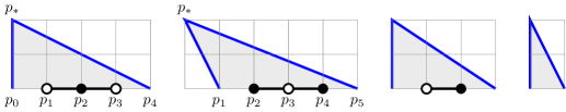
Figure 1. $A$ shapes: $A_{3}$, $\raise 0.65pt\hbox{$\kern-2.0pt\phantom{.}^{-}$}\kern-4.0ptA_{3}^{-}$, $A_{2}^{-}$, $A_{0}^{-}$

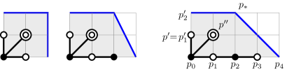
Figure 2. $D$ shapes: $D_{4}$, $D_{5}^{-}$, $D_{6}$

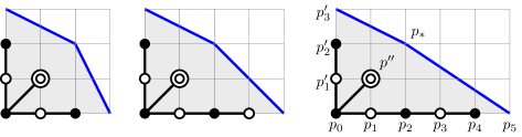
Figure 3. $E$ shapes: $\raise 0.65pt\hbox{$\kern-2.0pt\phantom{.}^{-}$}\kern-2.0ptE_{6}^{-}$, $\raise 0.65pt\hbox{$\kern-2.0pt\phantom{.}^{-}$}\kern-2.0ptE_{7}$, $\raise 0.65pt\hbox{$\kern-2.0pt\phantom{.}^{-}$}\kern-2.0ptE_{8}^{-}$

Figure 4. Type II shapes ${\widetilde{D}}_{8}$, ${\widetilde{E}}_{7}$ and ${\widetilde{E}}_{8}^{-}$

Definition 3.6.

Given a surface $(Y,C)$ of pure shape, we call the irreducible components of $C$ sides. If $(Y,C)$ is of type III there are two sides, we call them left and right and decompose $C=C_{1}+C_{2}$ correspondingly. If $(Y,C)$ is of type II there may be one side or no sides.

Let $L=-2(K_{Y}+C)$. We call a side $C^{\prime}$ long if $L.C^{\prime}=2$ or $4$, and short if $L.C^{\prime}=1$ or $3$.

In the type III cases illustrated in Figures 1, 2, 3, long sides have lattice length 2 and short sides have lattice length 1. In the type II cases illustrated in Figure 4, long sides have lattice length 4 and short sides have lattice length 3.

Within each polytope in Figures 1, 2, 3, 4 we draw the corresponding decorated Dynkin diagram, using the following rule.

Notation 3.7.

Given a surface of pure shape $(Y,C)$ defined torically by a polytope $P$ as above, mark a node for each lattice point on the boundary of of $P$ which is not contained in $C$, and join them with edges along the boundary. For any node that lies at a corner of $P$, add an additional internal node to the diagram and connect it to the corner node. We distinguish such internal nodes by circling them in our diagrams.

This process associates an $ADE$ (resp. ${\widetilde{A}}{\widetilde{D}}{\widetilde{E}}$) diagram to each of our torically-defined pure shapes of type III (resp. type II), but it does not give a bijective correspondence between diagrams and shapes. To fix this we also need to keep track of the parity. We color the nodes of a diagram lying at lattice length 2 from $p_{*}$ black, and the nodes lying at lattice length 1 from $p_{*}$ white. Internal nodes are always colored white.

In the type III cases, note that each diagram has a leftmost and rightmost node, which sit next to the left and right sides respectively. The length of the sides may be read off from the colors of these nodes: white nodes correspond to long sides and black nodes to short sides.

Notation 3.8.

For ease of reference, to each decorated Dynkin diagram we also associate a decorated Dynkin symbol, in a unique way. For the pure shapes, this is given by the name of the (undecorated) Dynkin diagram, with superscript minus signs on the left/right to denote the locations of short sides; as noted above, this can be read off from the colors of the nodes at the ends of the diagram. For instance, as illustrated in Figure 1, $A_{3}$ has two long sides, $\raise 0.65pt\hbox{$\kern-2.0pt\phantom{.}^{-}$}\kern-4.0ptA_{3}^{-}$ has two short sides, and $A_{2}^{-}$ has a long side on the left and a short side on the right. In type II cases, which have only one side, we place all decorations on the right by convention.

Remark 3.9.

With this notation, the two shapes $\raise 0.65pt\hbox{$\kern-2.0pt\phantom{.}^{-}$}\kern-4.0ptA_{2n-2}$ and $A_{2n-2}^{-}$ are identical up to labeling of the components of $C$. Where this labeling is unimportant, we will refer to these surfaces by the symbol $A_{2n-2}^{-}$, with the short side on the right. There are, however, some settings in which it will be important to keep track of the labels, such as when we come to study degenerations.

Remark 3.10.

Curiously, there is no ${\widetilde{E}}_{6}$ shape. In our ad hoc definition above, the process of adding internal nodes can only produce branches of length 2. This rules out Dynkin diagram ${\widetilde{E}}_{6}$, which has three branches of length 3. A deeper reason is that in Arnold’s classification of singularities [Arn72] the ${\widetilde{E}}_{7}$ and ${\widetilde{E}}_{8}$ singularities exist in all dimensions $\geq 2$, but ${\widetilde{E}}_{6}$ starts in dimension 3 and so cannot appear on a surface.

3B. Nontoric ${\widetilde{A}}$ shapes

In addition to the toric surfaces described above, there are also three nontoric ${\widetilde{A}}{\widetilde{D}}{\widetilde{E}}$ surfaces (type II) of pure shape. These are the ${\widetilde{A}}$ shapes, their decorated Dynkin diagrams and symbols are chosen to be compatible with moduli and degenerations, although they do not admit the same nice description in terms of polytopes as the toric shapes. They are illustrated in Figure 5.

(1) $\bm{{\widetilde{A}}_{2n-1}}$. The surface $Y$ is a cone over an elliptic curve and $C=0$, so there is no boundary. More precisely, let ${\mathcal{F}}$ be a line bundle of degree $n>0$ on an elliptic curve $E$, and let ${\widetilde{Y}}$ be the surface $\operatorname{Proj}_{E}({\mathcal{O}}\oplus{\mathcal{F}})$. Let $s,s_{\infty}$ be the zero, resp. infinity sections, and let $f\colon{\widetilde{Y}}\to Y$ be the contraction of the zero section. Then $f^{*}K_{Y}=K_{\widetilde{Y}}+s=-s_{\infty}$, so $-K_{Y}$ is ample with $K_{Y}^{2}=n$. If $B\in|-2K_{Y}|$ is a generic section then $p_{a}(B)=n+1$ and the map $B\to E$ has $2n$ points of ramification. Of course, the surface $Y$ is not toric. The double cover $X\to Y$ branched in $B$ is unramified at the singular point, and $X$ has two elliptic singularities. One has $R^{2}=2K_{Y}^{2}=2n$.

(2) $\bm{{\widetilde{A}}_{1}^{*}}$. The surface is the projective plane $Y={\mathbb{P}}^{2}$, the boundary $C$ is a smooth conic, and the branch curve $B$ is a possibly singular conic. If $B$ is smooth then the double cover $X={\mathbb{P}}^{1}\times{\mathbb{P}}^{1}$; if $B$ is two lines then $X={\mathbb{F}}_{2}^{0}={\mathbb{P}}(1,1,2)$ with $R$ passing through the singular point of $X$. We also include here as a degenerate subcase when ${\mathbb{P}}^{2}$ degenerates to $Y={\mathbb{F}}_{4}^{0}$. Then $X={\mathbb{F}}_{2}^{0}$ with $R$ not passing through the singular point.

(3) $\bm{{\widetilde{A}}_{0}^{-}}$. The surface is the quadratic cone $Y={\mathbb{P}}(1,1,2)$ with minimal resolution ${\widetilde{Y}}={\mathbb{F}}_{2}$. The strict preimage of $C$ on ${\widetilde{Y}}$ is a divisor in the linear system $|s+3f|$, where $s$ is the $(-2)$-section and $f$ is a fiber. The curve $C$ passes through the vertex of the cone and is smooth at that point. The branch curve $B$ is a hyperplane section disjoint from the vertex. The double cover is $X={\mathbb{P}}^{2}$ with an involution $(x,y,z)\mapsto(x,-y,z)$, and the boundary divisor is a smooth elliptic curve $y^{2}z=f_{3}(x,z)$.

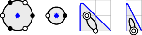
Figure 5. Nontoric type II ${\widetilde{A}}$ shapes: ${\widetilde{A}}_{5}$, ${\widetilde{A}}_{1}$, ${\widetilde{A}}_{1}^{*}$, ${\widetilde{A}}_{0}^{-}$

The surface $Y$ of shape ${\widetilde{A}}_{1}^{*}$ is obtained by a “corner smoothing” of a surface of toric shape $A_{1}$: the union of two lines $C_{1}+C_{2}$ in ${\mathbb{P}}^{2}$ is smoothed to a conic $C$. Similarly, ${\widetilde{A}}_{0}^{-}$ is obtained by a “corner smoothing” of $A_{0}^{-}$. We add the star in ${\widetilde{A}}_{1}^{*}$ to distinguish it from the ordinary ${\widetilde{A}}_{1}$ shape, which has no boundary.

Remark 3.11.

One observes that the ${\widetilde{A}}$ shapes cannot be toric because the Dynkin diagram is not a tree.

Remark 3.12.

With the single exception of ${\widetilde{A}}_{1}^{*}$, all of our decorated Dynkin graphs are bipartite: black and white nodes appear in alternating order.

3C. Primed shapes

Priming is a natural operation producing a new del Pezzo surface $({\overline{Y}}^{\prime},{\overline{C}}^{\prime})$ of index 2 from an old one $(Y,C)$. Let $I_{i}\simeq(y,x^{2})$ be an ideal with support at a smooth point $P_{i}\in C$ whose direction is transversal to $C$. A weighted blowup at $I_{i}$ is a composition of two ordinary blowups: at $P_{i}$ and at the point $P_{i}^{\prime}$ corresponding to the direction of $I_{i}$, followed by a contraction of an $(-2)$-curve, making an $A_{1}$ surface singularity at a point contained in the strict preimage $C^{\prime}$ of $C$. Weighted blowups of this form are the basis of the priming operation.

Definition 3.13.

Let $(Y,C)$ be an $ADE$ or ${\widetilde{A}}{\widetilde{D}}{\widetilde{E}}$ surface and let $P_{1},\dotsc,P_{k}\in C$ be distinct nonsingular points of $Y$ and $C$. Choose ideals $I_{i}\simeq(y,x^{2})$ with supports at $P_{i}$ and directions transversal to $C$ (the closed subschemes $\operatorname{Spec}{\mathcal{O}}_{Y}/I_{i}$ can be thought of as vectors). Let $k_{s}$ denote the number of points on side $C_{s}$, so $k=\sum k_{s}$. Define $f\colon Y^{\prime}\to Y$ to be the weighted blowup at $I=\prod_{i=1}^{k}I_{i}$ and let $C^{\prime}$ be the strict preimage of $C$. Let $F=\sum F_{i}$ be the sum of the exceptional divisors and $L^{\prime}=-2(K_{Y^{\prime}}+C^{\prime})$; note that $L^{\prime}$ is a line bundle since an $A_{1}$ singularity has index 2.

Assume that $L^{\prime}$ is big, nef, and semiample. Then the priming of $(Y,C)$ is defined to be the pair $({\overline{Y}}^{\prime},{\overline{C}}^{\prime})$ obtained by composing $f$ with the contraction $g\colon Y^{\prime}\to{\overline{Y}}^{\prime}$ given by $|NL^{\prime}|$, $N\gg 0$. The divisor ${\overline{C}}^{\prime}$ is defined to be the strict transform of $C$. The resulting pair $({\overline{Y}}^{\prime},{\overline{C}}^{\prime})$ is an $ADE$ or ${\widetilde{A}}{\widetilde{D}}{\widetilde{E}}$ surface of primed shape.

Remark 3.14.

Priming has a very simple geometric meaning for the pairs $(Y,C+\frac{1+\epsilon}{2}B)$. Let $B\in|L|$ be a curve such that $(Y,C+\frac{1+\epsilon}{2}B)$ is log canonical. By (3.3) the curve $B$ is transversal to $C$. In this case we take the ideals $I_{i}$ to be supported at some of the points $P_{i}\in B\cap C$, with the directions equal to the tangent directions of $B$ at $P_{i}$. Priming then produces a new pair $({\overline{Y}}^{\prime},{\overline{C}}^{\prime}+\frac{1+\epsilon}{2}{\overline{B}}^{\prime})$ which disconnects $B$ from $C$ at the points $P_{i}$. If a component of $C^{\prime}$ is completely disconnected from $B^{\prime}$ then it is contracted on ${\overline{Y}}^{\prime}$.

But it is on the double cover $\pi\colon(X,D+\epsilon R)\to(Y,C+\frac{1+\epsilon}{2}B)$ where the priming operation becomes the most natural and easiest to understand. The double cover $X^{\prime}$ of $Y^{\prime}$ branched in $B^{\prime}$ is an ordinary smooth blowup of $X$ at the points $Q_{i}=\pi^{-1}(P_{i})$. So on the cover we simply make $k$ ordinary blowups at some points $Q_{i}\in D\cap R$ in the boundary $D$ which are fixed by the involution, then apply the linear system $|NR^{\prime}|$, $N\gg 0$, provided that $R^{\prime}$ is big, nef and semiample, to obtain the primed pair $({\overline{X}}^{\prime},{\overline{D}}^{\prime}+\epsilon{\overline{R}}^{\prime})$. This disconnects $R$ from $D$ at the points $Q_{i}$. If a component of $D^{\prime}$ is completely disconnected from $R^{\prime}$ then it is contracted on ${\overline{X}}^{\prime}$.

Definition 3.15.

In terms of the pairs, we will call the above operation priming of an $ADE$(resp. ${\widetilde{A}}{\widetilde{D}}{\widetilde{E}}$) pair $(Y,C+\frac{1+\epsilon}{2}B)$, resp. priming of an $ADE$(resp. ${\widetilde{A}}{\widetilde{D}}{\widetilde{E}}$) double cover $(X,D+\epsilon R)$. The result is an $ADE$(resp. ${\widetilde{A}}{\widetilde{D}}{\widetilde{E}}$) pair/double cover of primed shape.

We reiterate that a priming only exists if $L^{\prime}$ is big, nef, and semiample. Below we will give a necessary and sufficient condition for existence of a priming that is easier to check; before that, however, we need to introduce some basic invariants.

Definition 3.16.

The basic numerical invariants of an $ADE$ or ${\widetilde{A}}{\widetilde{D}}{\widetilde{E}}$ surface $(Y,C)$, with polarization $L=-2(K_{Y}+C)$, are

1. the volume $v=L^{2}/2>0$,

2. the genus $g=\frac{1}{2}(K_{Y}+L)L-1\geq 0$,

3. the lengths $LC_{s}>0$ of the sides.

The Hilbert polynomial of $(Y,L)$ is $\chi(Y,xL)=vx^{2}+(v+1-g)x+1$. The Hilbert polynomials of $(C_{s},L)$ are $2x+1$ for a long side and $x+1$ for a short side. It is immediate to compute these invariants for the pure shapes. We list them in the highlighted rows of Tables 2 and 3.

Lemma 3.17.

With notation as in Definition 3.13:

1. For the main divisors, one has

   $$C^{\prime}=f^{*}C-F,\quad K_{Y^{\prime}}=f^{*}K_{Y}+2F,\quad L^{\prime}=f^{*}L-2F,\quad K_{Y^{\prime}}+L^{\prime}=f^{*}(K_{Y}+L).$$

2. The basic invariants change as follows:

   $$L^{\prime}{}^{2}/2=L^{2}/2-k,\quad g(L^{\prime})=g(L),\quad L^{\prime}C_{s}^{\prime}=LC_{s}-k_{s}.$$

Theorem 3.18 (Allowed primings).

Let $(Y,C)$ be an $ADE$ or ${\widetilde{A}}{\widetilde{D}}{\widetilde{E}}$ surface of pure shape, as defined in sections 3A and 3B, and $I_{1},\dotsc,I_{k}$ a collection of ideals as in Definition 3.13. Then a necessary and sufficient condition for a priming to exist is: $L^{\prime}{}^{2}>0$ and $L^{\prime}C^{\prime}_{s}\geq 0$ for the sides $C_{s}$. Under these conditions, $L^{\prime}$ is big, nef, and semiample, and contracts $Y^{\prime}$ to a normal surface ${\overline{Y}}^{\prime}$ with ample Cartier divisor $-2(K_{{\overline{Y}}^{\prime}}+{\overline{C}}^{\prime})$.

Proof.

The conditions $L^{\prime}{}^{2}>0$ and $L^{\prime}C^{\prime}_{s}\geq 0$ are necessary since $L^{\prime}$ is big and nef. Now assume that they are satisfied. We exclude ${\widetilde{A}}_{2n-1}$ since its boundary is empty and no primings are possible. We can also exclude the shapes of volume 1, which are $A_{0}^{-}$ and ${\widetilde{A}}_{0}^{-}$. By (3.17) one has

$$\frac{1}{2}L^{\prime}=(K_{Y^{\prime}}+L^{\prime})+C^{\prime}=f^{*}(K_{Y}+L)+C^{\prime}.$$

Thus, if $K_{Y}+L$ is nef then $L^{\prime}$ is nef. One checks that for all the pure shapes except for $A_{1}$ and ${\widetilde{A}}_{1}^{*}$ the divisor $K_{Y}+L$ is nef. Indeed, the surfaces of $A_{2n-1}$, $A^{-}_{2n-2}$, $\raise 0.65pt\hbox{$\kern-2.0pt\phantom{.}^{-}$}\kern-4.0ptA^{-}_{2n-3}$ and ${\widetilde{E}}_{7}$, ${\widetilde{E}}_{8}^{-}$ shapes have Picard rank 1, so $K_{Y}+L$ is nef iff the genus $g\geq 0$, i.e. all except $A_{1}$ and the excluded $A_{0}^{-}$. For the $D_{4},{\widetilde{D}}_{4}$ shapes one has $K_{Y}+L=0$. For the other $D_{2n}$, $D^{-}_{2n-1}$, ${\widetilde{D}}_{2n}$ shapes $K_{Y}+L$ gives a ${\mathbb{P}}^{1}$-fibration. Finally, for the $E$ shapes the divisor $K_{Y}+L$ is big and nef: for $\raise 0.65pt\hbox{$\kern-2.0pt\phantom{.}^{-}$}\kern-2.0ptE^{-}_{6}$ it is ample, for $\raise 0.65pt\hbox{$\kern-2.0pt\phantom{.}^{-}$}\kern-2.0ptE_{7}$ it contracts the left side $C_{1}$ to an ${\widetilde{E}}_{7}$ surface, and for $\raise 0.65pt\hbox{$\kern-2.0pt\phantom{.}^{-}$}\kern-2.0ptE_{8}^{-}$ it contracts the right side $C_{2}$ to an ${\widetilde{E}}_{8}^{-}$ surface.

The remaining shapes $A_{1}$ and ${\widetilde{A}}_{1}^{*}$ are easy to check directly. In both cases $Y={\mathbb{P}}^{2}$ and $C$ is a conic: two lines for $A_{1}$ and a smooth conic for ${\widetilde{A}}_{1}^{*}$. The divisor $L^{\prime}$ is big and nef and contracts a $(-1)$-curve $E^{\prime}$, the strict preimage of a line $E$ with the direction of the ideal $I$, to a surface of shape $A_{0}^{-}$, resp. ${\widetilde{A}}_{0}^{-}$.

Since $\frac{1}{2}L^{\prime}$ is of the form $-(K_{Y}^{\prime}+C^{\prime})$, if it is big and nef then it is automatically semiample, see e.g. [Fuj12, Thm.6.1]. This concludes the proof. ∎

Corollary 3.19.

The shapes $A_{2n-1}$, $D_{2n}$, ${\widetilde{D}}_{2n}$, ${\widetilde{E}}_{7}$ can be primed a maximum of 4 times, shapes ${\widetilde{A}}_{2n-2}^{-}$, ${\widetilde{D}}_{2n-1}^{-}$, ${\widetilde{E}}_{8}^{-}$ 3 times, and $\raise 0.65pt\hbox{$\kern-2.0pt\phantom{.}^{-}$}\kern-4.0ptA^{-}_{2n-2}$, $\raise 0.65pt\hbox{$\kern-2.0pt\phantom{.}^{-}$}\kern-2.0ptE_{6}^{-}$, $\raise 0.65pt\hbox{$\kern-2.0pt\phantom{.}^{-}$}\kern-2.0ptE_{8}^{-}$ 2 times each.

Remark 3.20.

As we can see from the above proof, the cases $A_{1}^{\prime}=A_{0}^{-}$ and $({\widetilde{A}}_{1}^{*})^{\prime}={\widetilde{A}}_{0}^{-}$ are special. Also, as we will see below, the dimension of the moduli space of pairs in these cases drops after priming, but in all other cases it is preserved. For these reasons, and to avoid redundancy in our naming scheme, we do not allow primings of $A_{1}$ and ${\widetilde{A}}_{1}^{*}$.

We associate decorated Dynkin diagrams and symbols to primed shapes by modifying those of the corresponding pure shapes, as follows. Recall that, in the pure Type III cases, each diagram has a leftmost and rightmost node, which sit next to the left and right sides, and these nodes are colored white/black if and only if the corresponding side is long/short.

Notation 3.21.

For an $ADE$ shape, when priming on a long side once we circle the corresponding white node, and when priming a second time we also circle the neighboring black node. In the Dynkin symbol we add a prime, resp. double prime on the left or right, depending on whether we are priming at a point of the left side $C_{1}$ or the right side $C_{2}$. When priming on a short side, we circle the corresponding black node once and turn the $-$ superscript into a $+$ superscript (visually $-$ and ^′ gives $+$).

For an ${\widetilde{A}}{\widetilde{D}}{\widetilde{E}}$ shape, we add up to 4 primes to the Dynkin symbol for a long side in ${\widetilde{D}}_{2n}$ and ${\widetilde{E}}_{7}$. We also turn ${\widetilde{E}}_{8}^{-}$ into ${\widetilde{E}}_{8}^{+}$ before adding up to two more primes. In the corresponding decorated diagrams, we circle one node for each prime using the following rule: first circle black nodes at the ends of the diagram, then white nodes at the ends of the diagram, then finally black nodes connected to circled white ones.

Remark 3.22.

We note two pieces of mild ambiguity in this notation. The first is that the decorated diagrams for the two shapes $\kern-2.0pt\phantom{.}^{\prime\prime}\kern-2.0pt\kern-1.0ptA_{3}^{\prime},\kern-2.0pt\phantom{.}^{\prime}\kern-2.0pt\kern-1.0ptA_{3}^{\prime\prime}$ and also for $\kern-2.0pt\phantom{.}^{\prime\prime}\kern-2.0ptD^{\prime}_{4},\kern-2.0pt\phantom{.}^{\prime}\kern-2.0ptD^{\prime\prime}_{4}$ are the same, so the diagram in these cases does not distinguish left and right sides. In practice this won’t cause a problem: if we need to distinguish sides in these cases we will use the Dynkin symbols $\kern-2.0pt\phantom{.}^{\prime\prime}\kern-2.0pt\kern-1.0ptA_{3}^{\prime},\kern-2.0pt\phantom{.}^{\prime}\kern-2.0pt\kern-1.0ptA_{3}^{\prime\prime}$, resp. $\kern-2.0pt\phantom{.}^{\prime\prime}\kern-2.0ptD^{\prime}_{4},\kern-2.0pt\phantom{.}^{\prime}\kern-2.0ptD^{\prime\prime}_{4}$.

The decorated diagrams for the shapes $\kern-2.0pt\phantom{.}^{\prime}\kern-2.0pt\kern-1.0ptA_{2}^{+}$ and $\kern-2.0pt\phantom{.}^{\prime\prime}\kern-2.0pt\kern-1.0ptA_{2}^{-}$ are also identical. In fact, in this case we find that the $ADE$ surfaces $\kern-2.0pt\phantom{.}^{\prime}\kern-2.0pt\kern-1.0ptA_{2}^{+}$ and $\raise 0.65pt\hbox{$\kern-2.0pt\phantom{.}^{-}$}\kern-4.0ptA_{2}^{\prime\prime}$ are isomorphic, so this is just another instance of the diagram not distinguishing left and right sides. These surfaces are obtained by priming $\kern-2.0pt\phantom{.}^{\prime}\kern-2.0pt\kern-1.0ptA_{2}^{-}$ and $\raise 0.65pt\hbox{$\kern-2.0pt\phantom{.}^{-}$}\kern-4.0ptA_{2}^{\prime}$, respectively, once on the right and a surface of $\kern-2.0pt\phantom{.}^{\prime}\kern-2.0pt\kern-1.0ptA_{2}^{-}$ shape is left/right symmetric (in fact it has a toric description which makes this symmetry apparent, see Lemma 3.25 and Figure 7). One way to think of this symmetry is to consider $\kern-2.0pt\phantom{.}^{\prime}\kern-2.0pt\kern-1.0ptA_{2}^{-}=\raise 0.65pt\hbox{$\kern-2.0pt\phantom{.}^{-}$}\kern-4.0ptA_{2}^{\prime}$ as a symmetric $\raise 0.65pt\hbox{$\kern-2.0pt\phantom{.}^{-}$}\kern-2.0ptD_{2}^{-}$ shape.

Remark 3.23.

If we wish to refer to an $ADE$ or ${\widetilde{A}}{\widetilde{D}}{\widetilde{E}}$ surface with an unspecified decoration (i.e. either undecorated or one of $-,\prime,{\prime\prime},+$), we will use a question mark decoration $\mbox{}^{?}$. For example, $A_{2n-1}^{?}$ refers to one of the surfaces $A_{2n-1}$, $A_{2n-1}^{\prime}$, or $A_{2n-1}^{\prime\prime}$, while $\kern-2.0pt\phantom{.}^{\prime}\kern-2.0ptA_{2n-2}^{?}$ refers to one of the surfaces $\kern-2.0pt\phantom{.}^{\prime}\kern-2.0ptA_{2n-2}^{-}$ or $\kern-2.0pt\phantom{.}^{\prime}\kern-2.0ptA_{2n-2}^{+}$.

Note that circled white nodes can denote either internal nodes or long sides on which a single priming has taken place. This apparent notational ambiguity will be explained in the following subsection.

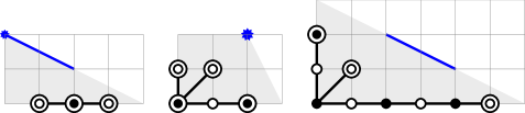
Figure 6. Decorated Dynkin diagrams for shapes $\kern-2.0pt\phantom{.}^{\prime\prime}\kern-2.0pt\kern-1.0ptA_{3}^{\prime}$, $\kern-2.0pt\phantom{.}^{\prime\prime}\kern-2.0ptD_{5}^{+}$, ${\widetilde{E}}_{8}^{+}{}^{\prime}$

Example 3.24.

In Fig. 6 we give several examples of such diagrams. The surfaces in these cases are not toric. However, we can still use pseudo-toric pictures to indicate the lengths ${\overline{L}}\,{\overline{C}}^{\prime}_{s}$ of the sides and the sides $C^{\prime}_{s}$ which are contracted by $Y^{\prime}\to{\overline{Y}}^{\prime}$. The volume of the surface is the volume of the polytope minus the number of primes, i.e. additional circles in the diagram as compared to a pure shape.

We list all the resulting 43 $ADE$ and 17 ${\widetilde{A}}{\widetilde{D}}{\widetilde{E}}$ shapes and their basic invariants in Tables 2 and 3. The pure shapes are highlighted. Note that this table does not distinguish between left and right sides of $A$-shapes (see Remark 3.9), so e.g. $A_{2n-2}^{-}$ and $\raise 0.65pt\hbox{$\kern-2.0pt\phantom{.}^{-}$}\kern-4.0ptA_{2n-2}$ are listed as the same surface. The column for the singularities is explained in section 3E.

$$\begin{array}[]{ll|llll}\text{shape}&\min(n)&\text{volume}&\text{genus}&LC_{s}&\text{sings in }\rm nonklt(Y,C)\\ \hline\cr A_{2n-1}&1&2n&n-1&2,2&(n)\\ A^{\prime}_{2n-1}&2&2n-1&n-1&2,1&(n),A_{1}\\ \kern-2.0pt\phantom{.}^{\prime}\kern-2.0pt\kern-1.0ptA_{2n-1}^{\prime}&2&2n-2&n-1&1,1&A_{1},(n),A_{1}\\ A_{2n-1}^{\prime\prime}&2&2n-2&n-1&2&(n,2;2^{2})\\ \kern-2.0pt\phantom{.}^{\prime}\kern-2.0pt\kern-1.0ptA_{2n-1}^{\prime\prime}&2&2n-3&n-1&1&A_{1},(n,2;2^{2})\\ \kern-2.0pt\phantom{.}^{\prime\prime}\kern-2.0pt\kern-1.0ptA_{2n-1}^{\prime\prime}&3&2n-4&n-1&&(2^{2};2,n,2;2^{2})\\ \hline\cr A_{2n-2}^{-}&1&2n-1&n-1&2,1&(n,2),A_{1}\\ \kern-2.0pt\phantom{.}^{\prime}\kern-2.0pt\kern-1.0ptA_{2n-2}^{-}&2&2n-2&n-1&1,1&A_{1},(n,2),A_{1}\\ A^{+}_{2n-2}&2&2n-2&n-1&2&(n,2,2;2^{2})\\ \kern-2.0pt\phantom{.}^{\prime}\kern-2.0pt\kern-1.0ptA_{2n-2}^{+}&2&2n-3&n-1&1&A_{1},(n,2,2;2^{2})\\ \kern-2.0pt\phantom{.}^{\prime\prime}\kern-2.0pt\kern-1.0ptA_{2n-2}^{-}&2&2n-3&n-1&1&(2^{2};2,n,2),A_{1}\\ \kern-2.0pt\phantom{.}^{\prime\prime}\kern-2.0pt\kern-1.0ptA_{2n-2}^{+}&3&2n-4&n-1&&(2^{2};2,n,2,2;2^{2})\\ \hline\cr\raise 0.65pt\hbox{$\kern-2.0pt\phantom{.}^{-}$}\kern-4.0ptA_{2n-3}^{-}&2&2n-2&n-1&1,1&A_{1},(2,n,2),A_{1}\\ \raise 0.65pt\hbox{$\kern-2.0pt\phantom{.}^{-}$}\kern-4.0ptA_{2n-3}^{+}&2&2n-3&n-1&1&A_{1},(2,n,2,2;2^{2})\\ \raise 0.65pt\hbox{$\kern-2.0pt\phantom{.}^{+}$}\kern-4.0ptA_{2n-3}^{+}&3&2n-4&n-1&&(2^{2};2,2,n,2,2;2^{2})\\ \hline\cr D_{2n}&2&2n&n-1&2,2&\\ D_{2n}^{\prime}&2&2n-1&n-1&2,1&A_{1}\\ \kern-2.0pt\phantom{.}^{\prime}\kern-2.0ptD_{2n}&2&2n-1&n-1&1,2&A_{1}\\ \kern-2.0pt\phantom{.}^{\prime}\kern-2.0ptD_{2n}^{\prime}&2&2n-2&n-1&1,1&2A_{1}\\ D_{2n}^{\prime\prime}&2&2n-2&n-1&2&(2;2^{2})\\ \kern-2.0pt\phantom{.}^{\prime\prime}\kern-2.0ptD_{2n}&2&2n-2&n-1&2&(2^{2};n)\\ \kern-2.0pt\phantom{.}^{\prime}\kern-2.0ptD_{2n}^{\prime\prime}&2&2n-3&n-1&1&A_{1},(2;2^{2})\\ \kern-2.0pt\phantom{.}^{\prime\prime}\kern-2.0ptD_{2n}^{\prime}&2&2n-3&n-1&1&(2^{2};n),A_{1}\\ \kern-2.0pt\phantom{.}^{\prime\prime}\kern-2.0ptD_{2n}^{\prime\prime}&3&2n-4&n-1&&(2^{2};n,2;2^{2})\\ \hline\cr D_{2n-1}^{-}&3&2n-1&n-1&2,1&(2),A_{1}\\ \kern-2.0pt\phantom{.}^{\prime}\kern-2.0ptD_{2n-1}^{-}&3&2n-2&n-1&1,1&A_{1},(2),A_{1}\\ D_{2n-1}^{+}&3&2n-2&n-1&2&(2,2;2^{2})\\ \kern-2.0pt\phantom{.}^{\prime}\kern-2.0ptD_{2n-1}^{+}&3&2n-3&n-1&1&A_{1},(2,2;2^{2})\\ \kern-2.0pt\phantom{.}^{\prime\prime}\kern-2.0ptD_{2n-1}^{-}&3&2n-3&n-1&1&(2^{2};n,2),A_{1}\\ \kern-2.0pt\phantom{.}^{\prime\prime}\kern-2.0ptD_{2n-1}^{+}&3&2n-4&n-1&&(2^{2};n,2,2;2^{2})\\ \hline\cr\raise 0.65pt\hbox{$\kern-2.0pt\phantom{.}^{-}$}\kern-2.0ptE_{6}^{-}&&6&3&1,1&A_{1},(3),A_{1}\\ \raise 0.65pt\hbox{$\kern-2.0pt\phantom{.}^{-}$}\kern-2.0ptE_{6}^{+}&&5&3&1&A_{1},(3,2;2^{2})\\ \raise 0.65pt\hbox{$\kern-2.0pt\phantom{.}^{+}$}\kern-2.0ptE_{6}^{+}&&4&3&&(2^{2};2,3,2;2^{2})\\ \hline\cr\raise 0.65pt\hbox{$\kern-2.0pt\phantom{.}^{-}$}\kern-2.0ptE_{7}&&7&3&1,2&A_{1}\\ \raise 0.65pt\hbox{$\kern-2.0pt\phantom{.}^{-}$}\kern-2.0ptE_{7}^{\prime}&&6&3&1,1&2A_{1}\\ \raise 0.65pt\hbox{$\kern-2.0pt\phantom{.}^{+}$}\kern-2.0ptE_{7}&&6&3&2&(2^{2};2)\\ \raise 0.65pt\hbox{$\kern-2.0pt\phantom{.}^{+}$}\kern-2.0ptE_{7}^{\prime}&&5&3&1&(2^{2};2),A_{1}\\ \raise 0.65pt\hbox{$\kern-2.0pt\phantom{.}^{-}$}\kern-2.0ptE_{7}^{\prime\prime}&&5&3&1&A_{1},(2,3,2)\\ \raise 0.65pt\hbox{$\kern-2.0pt\phantom{.}^{+}$}\kern-2.0ptE_{7}^{\prime\prime}&&4&3&&(2^{2};2,3;2^{2})\\ \hline\cr\raise 0.65pt\hbox{$\kern-2.0pt\phantom{.}^{-}$}\kern-2.0ptE_{8}^{-}&&8&4&1,1&2A_{1}\\ \raise 0.65pt\hbox{$\kern-2.0pt\phantom{.}^{-}$}\kern-2.0ptE_{8}^{+}&&7&4&1&A_{1},(3;2^{2})\\ \raise 0.65pt\hbox{$\kern-2.0pt\phantom{.}^{+}$}\kern-2.0ptE_{8}^{-}&&7&4&1&(2^{2};2),A_{1}\\ \raise 0.65pt\hbox{$\kern-2.0pt\phantom{.}^{+}$}\kern-2.0ptE_{8}^{+}&&6&4&&(2^{2};2,3;2^{2})\\ \hline\cr\end{array}$$

Table 2. All $ADE$ shapes

$$\begin{array}[]{ll|llll}\text{shape}&\min(n)&\text{volume}&\text{genus}&LC&\text{sings in }\rm nonklt(Y,C)\\ \hline\cr\rule{0.0pt}{12.05553pt}{\widetilde{A}}_{2n-1}&1&2n&n+1&&\text{elliptic}\\ \hline\cr\rule{0.0pt}{12.05553pt}{\widetilde{A}}_{1}^{*}&&2&0&4&\\ \hline\cr\rule{0.0pt}{12.05553pt}{\widetilde{A}}_{0}^{-}&&1&0&3&A_{1}\\ \hline\cr\rule{0.0pt}{12.05553pt}{\widetilde{D}}_{2n}&2&2n&n-1&4&\\ {\widetilde{D}}_{2n}^{\prime}&2&2n-1&n-1&3&A_{1}\\ {\widetilde{D}}_{2n}^{\prime\prime}&2&2n-2&n-1&2&2A_{1}\\ {\widetilde{D}}_{2n}^{\prime\prime\prime}&2&2n-3&n-1&1&3A_{1}\\ {\widetilde{D}}_{2n}^{\prime\prime\prime\prime}&3&2n-4&n-1&&(n;2^{4})\\ \hline\cr\rule{0.0pt}{12.05553pt}{\widetilde{E}}_{7}&&8&3&4&\\ {\widetilde{E}}_{7}^{\prime}&&7&3&3&A_{1}\\ {\widetilde{E}}_{7}^{\prime\prime}&&6&3&2&2A_{1}\\ {\widetilde{E}}_{7}^{\prime\prime\prime}&&5&3&1&3A_{1}\\ {\widetilde{E}}_{7}^{\prime\prime\prime\prime}&&4&3&&(3;2^{4})\\ \hline\cr\rule{0.0pt}{12.05553pt}{\widetilde{E}}_{8}^{-}&&9&4&3&A_{1}\\ {\widetilde{E}}_{8}^{+}&&8&4&2&2A_{1}\\ {\widetilde{E}}_{8}^{+\prime}&&7&4&1&3A_{1}\\ {\widetilde{E}}_{8}^{+{\prime\prime}}&&6&4&&(3;2^{4})\\ \hline\cr\end{array}$$

Table 3. All ${\widetilde{A}}{\widetilde{D}}{\widetilde{E}}$ shapes

3D. Primed shapes which are toric

We observe that some of the primed shapes also admit toric descriptions. This provides an explanation for a piece of notational ambiguity mentioned in the previous subsection: the priming operation on a long edge (white node) may be interpreted as modifying the diagram to make that node internal in the toric representation.

$$\begin{array}[]{lc|c|lll}\text{shape}&\min(n)&p_{*}&\text{polytope vertices}\\ \hline\cr\kern-2.0pt\phantom{.}^{\prime}\kern-2.0pt\kern-1.0ptA_{2n-1}&2&(2,2)&(2,2),(0,1),(0,0),(2n-2,0)\\ \kern-2.0pt\phantom{.}^{\prime}\kern-2.0pt\kern-1.0ptA_{2n-2}^{-}&2&(2,2)&(2,2),(0,1),(0,0),(2n-3,0)\\ \kern-2.0pt\phantom{.}^{\prime}\kern-2.0pt\kern-1.0ptA_{2n-1}^{\prime}&3&(2,2)&(2,2),(0,1),(0,0),(2n-4,0),(n,1)\\ D_{2n}^{\prime}&3&(2,2)&(2,2),(0,2),(0,0),(2n-4,0),(n,1)\\ \hline\cr\end{array}$$

Table 4. Polytopes for the toric primed shapes

Lemma 3.25.

The shapes $\kern-2.0pt\phantom{.}^{\prime}\kern-2.0pt\kern-1.0ptA_{2n-1}$, $\kern-2.0pt\phantom{.}^{\prime}\kern-2.0pt\kern-1.0ptA_{2n-2}^{-}$, $D^{\prime}_{2n}$, $\kern-2.0pt\phantom{.}^{\prime}\kern-2.0pt\kern-1.0ptA_{2n-1}^{\prime}$ are toric and can be represented by the polytopes listed in Table 4 and illustrated in Figs. 7 and 8.

Proof.

In these cases we can choose the ideals $I_{i}$ to be torus invariant, with $\operatorname{Supp}I_{i}$ corresponding to vertices of the polytopes of the pure shapes $A_{2n-1}$, $A_{2n-2}^{-}$, $D_{2n}$, and $I_{i}$ pointing in the directions of the respective sides. Then the blown up surface $Y^{\prime}={\overline{Y}}^{\prime}$ is also toric, for the polytope obtained from the old polytope by cutting corners, as in Table 4 and Fig. 8. ∎

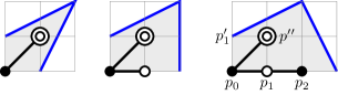
Figure 7. Toric $\kern-2.0pt\phantom{.}^{\prime}\kern-2.0pt\kern-1.0ptA$ shapes: $\kern-2.0pt\phantom{.}^{\prime}\kern-2.0pt\kern-1.0ptA_{2}^{-}=\raise 0.65pt\hbox{$\kern-2.0pt\phantom{.}^{-}$}\kern-4.0ptA_{2}^{\prime}=\raise 0.65pt\hbox{$\kern-2.0pt\phantom{.}^{-}$}\kern-2.0ptD_{2}^{-}$, $\kern-2.0pt\phantom{.}^{\prime}\kern-2.0pt\kern-1.0ptA_{3}$, $\kern-2.0pt\phantom{.}^{\prime}\kern-2.0pt\kern-1.0ptA_{4}^{-}$

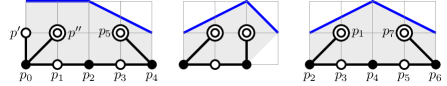
Figure 8. Toric $D^{\prime}$ and $\kern-2.0pt\phantom{.}^{\prime}\kern-2.0pt\kern-1.0ptA^{\prime}$ shapes: $D^{\prime}_{8}$, $\kern-2.0pt\phantom{.}^{\prime}\kern-2.0pt\kern-1.0ptA^{\prime}_{5}$, $\kern-2.0pt\phantom{.}^{\prime}\kern-2.0pt\kern-1.0ptA^{\prime}_{7}$

Remark 3.26.

For other primed shapes, the surfaces are generally not toric but toric surfaces do appear for certain special directions of the ideals being blown up. Some of them are shown in Fig. 9.

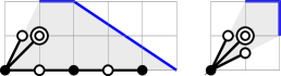
Figure 9. Some special toric surfaces in shapes $\kern-2.0pt\phantom{.}^{\prime}\kern-2.0ptD_{7}^{-}$, $\kern-2.0pt\phantom{.}^{\prime}\kern-2.0ptD_{4}^{\prime}$

3E. Singularities of $ADE$ and ${\widetilde{A}}{\widetilde{D}}{\widetilde{E}}$ surfaces

Theorem 3.27 (Singularities).

Let $(Y,C)$ be a surface of pure shape $\neq A_{1},{\widetilde{A}}_{1}^{*}$. With notation as in Definition 3.13, when priming $(Y,C)$ to $({\overline{Y}}^{\prime},{\overline{C}}^{\prime})$ the only curves contracted by $g\colon Y^{\prime}\to{\overline{Y}}^{\prime}$ are:

1. The sides $C^{\prime}_{s}$ with $L^{\prime}C^{\prime}_{s}=0$. These contract to $\rm nonklt({\overline{Y}}^{\prime},{\overline{C}}^{\prime})$.

2. A collection of $(-2)$ curves disjoint from $C^{\prime}$. These contract to Du Val singularities disjoint from $\rm nonklt(Y,C)$.

Proof.

Let $E^{\prime}$ be a curve with $L^{\prime}E^{\prime}=0$. As in the proof of Theorem 3.18, if $K_{Y}+L$ is nef and $E^{\prime}\neq C^{\prime}_{s}$ then $(K_{Y^{\prime}}+L^{\prime})E^{\prime}=0$, so $K_{Y^{\prime}}E^{\prime}=0$. Since $E^{\prime}$ is disjoint from the boundary, it lies in the smooth part of $Y^{\prime}$. We have $E^{\prime}{}^{2}<0$, and by the genus formula the only possibility is $E^{\prime}\simeq{\mathbb{P}}^{1}$ with $E^{\prime}{}^{2}=-2$. ∎

Corollary 3.28.

The singularities of the $ADE$ and ${\widetilde{A}}{\widetilde{D}}{\widetilde{E}}$ surfaces $(Y,C)$ lying in the nonklt locus of $(Y,C)$ depend only on the shape and are those listed in the last column of Tables 2 and 3.

Notation 3.29.

In Tables 2 and 3 we use the following notation for singularities. We denote simple nodes by the usual $A_{1}$. For cyclic quotient singularities, whose resolutions are a chain of curves, we use the notation $(n_{1},n_{2},\ldots,n_{k})$, where $-n_{i}$ is the self-intersection number of the $i$th curve in the chain; note that $(2,2,\ldots,2)$ corresponds to the Du Val singularity $A_{n}$. For more complicated singularities, whose resolution is not necessarily a chain of curves, we use the following notation: $(n_{1},n_{2},\ldots,n_{k};2^{2})$ denotes a singularity obtained by contracting a configuration of exceptional curves with the first dual graph in Fig. 10. Note that this includes Du Val singularities of type $D_{n}$, which are denoted by $(2,2,\ldots,2;2^{2})$.

Figure 10. Singularities $(n_{1},n_{2},\ldots,n_{k};2^{2})$ and $(2^{2};n_{1},n_{2},\ldots,n_{k};2^{2})$

Finally, we will use the expression $(2^{2};n_{1},n_{2},\ldots,n_{k};2^{2})$ to denote a singularity obtained by contracting a configuration of exceptional curves with the second dual graph in Fig. 10. Two apparently degenerate cases of this notation are $A_{1}=(2)$ and $(n;2^{2})=(2,n,2)$; we nonetheless use both notations, as it is useful to make a distinction when we discuss double covers. We will also often use $(n;2^{4})$ in place of $(2^{2};n;2^{2})$. Separately note that for $n=1$ the “singularities” $(n)$ and $(n,2)$ are in fact smooth points.

For completeness, we also note the corresponding singularities on the double covers. The double cover of a simple node $A_{1}$ is always a smooth point, and the double cover of a cyclic quotient singularity $(n_{1},n_{2},\ldots,n_{k})$ is always a pair of cyclic quotient singularities with the same resolution; this explains why we draw a distinction between $A_{1}$, which has smooth double cover, and $(2)$, which has double cover a pair of $(2)$ singularities.

The double cover of a singularity of type $(n_{1},n_{2},\ldots,n_{k};2^{2})$ is a cyclic quotient singularity $(n_{1},n_{2},\ldots,n_{k-1},2n_{k}-2,n_{k-1},\ldots,n_{1})$; this explains the second degenerate piece of notation, as $(2,n,2)$ has double cover a pair of $(2,n,2)$ singularities, and $(n;2^{2})$ has double cover a single $(2n-2)$ singularity. Finally, the double cover of a $(2^{2};n_{1},n_{2},\ldots,n_{k};2^{2})$ singularity, for $k\geq 2$, is a cusp singularity whose resolution is a cycle of rational curves with the negatives of self-intersections $(2n_{1}-2,n_{2},\ldots,n_{k-1},2n_{k}-2,n_{k-1},\ldots,n_{2})$ ordered cyclically, and the double cover of an $(n;2^{4})$ singularity is a simple elliptic singularity whose resolution is a smooth elliptic curve with the minus self-intersection $2n-4$.

3F. Recovering a precursor of pure shape

The aim of this subsection is to explore to what extent the priming operation is reversible. In other words, given an $ADE$ or ${\widetilde{A}}{\widetilde{D}}{\widetilde{E}}$ surface of primed shape, can we uniquely recover the surface of pure shape from which it was obtained by priming?

Lemma 3.30 (Non-redundancy).

When distinguishing the left and right sides, the only redundant case in the decorated Dynkin symbol notation for the shapes is $\kern-2.0pt\phantom{.}^{\prime}\kern-2.0pt\kern-1.0ptA^{-}_{2}=\raise 0.65pt\hbox{$\kern-2.0pt\phantom{.}^{-}$}\kern-4.0ptA^{\prime}_{2}$, for which also a symmetric but degenerate notation $\raise 0.65pt\hbox{$\kern-2.0pt\phantom{.}^{-}$}\kern-2.0ptD^{-}_{2}$ may be used. (See Remark 3.22. Recall also that $A_{1}^{\prime}=A_{0}^{-}$, $\kern-2.0pt\phantom{.}^{\prime}\kern-2.0pt\kern-1.0ptA_{1}=\raise 0.65pt\hbox{$\kern-2.0pt\phantom{.}^{-}$}\kern-4.0ptA_{0}$, and $({\widetilde{A}}_{1}^{*})^{\prime}={\widetilde{A}}_{0}^{-}$; for this reason we do not allow primings of $A_{1}$ and ${\widetilde{A}}_{1}^{*}$.)

When not distinguishing the left and right sides, there are also the cases coming from the ${\mathbb{Z}}_{2}$ symmetry of $A_{2n-1}$, $\raise 0.65pt\hbox{$\kern-2.0pt\phantom{.}^{-}$}\kern-4.0ptA_{2n-3}^{-}$, $\raise 0.65pt\hbox{$\kern-2.0pt\phantom{.}^{-}$}\kern-2.0ptD_{2}^{-}$, $D_{4}$, and $\raise 0.65pt\hbox{$\kern-2.0pt\phantom{.}^{-}$}\kern-2.0ptE_{6}^{-}$: $\kern-2.0pt\phantom{.}^{\prime}\kern-2.0pt\kern-1.0ptA_{5}=A_{5}^{\prime}$, $D_{4}^{\prime}=\kern-2.0pt\phantom{.}^{\prime}\kern-2.0ptD_{4}$, $E_{6}^{-}=\raise 0.65pt\hbox{$\kern-2.0pt\phantom{.}^{-}$}\kern-2.0ptE_{6}$, etc., including $\kern-2.0pt\phantom{.}^{\prime\prime}\kern-2.0pt\kern-1.0ptA_{2}^{-}=\kern-2.0pt\phantom{.}^{\prime}\kern-2.0pt\kern-1.0ptA_{2}^{+}$. (See Remarks 3.9 and 3.22.)

Proof.

By Tables 2 and 3, most of the shapes are already distinguished by the main invariants and singularities. The only exception is $D_{2n}^{\prime}$ and $\kern-2.0pt\phantom{.}^{\prime}\kern-2.0ptD_{2n}$ for $2n\geq 6$. However, in these cases the sheaf $K_{Y}+L$ gives a ${\mathbb{P}}^{1}$-fibration. The left side $C_{1}$ is a bisection of this fibration and $C_{2}$ lies in a fiber, so the two primings are not isomorphic. ∎

Definition 3.31.

Let $f\colon{\widetilde{Y}}\to Y$ be the minimal resolution of an $ADE$ or ${\widetilde{A}}{\widetilde{D}}{\widetilde{E}}$ surface $(Y,C)$. Let ${\widetilde{C}}_{s}$ be the strict transforms on ${\widetilde{Y}}$ of the components $C_{s}$ of $C$, and let $F_{i}$ be the $f$-exceptional curves. Let $C^{\perp}:=\langle C_{s},F_{i}\rangle^{\perp}\subset\operatorname{Pic}{\widetilde{Y}}$ and let $\Lambda_{0}:=C^{\perp}\cap B^{\perp}$. Denote by $\Delta^{(2)}_{0}$ the set of $(-2)$ vectors in $\Lambda_{0}$, by $\Lambda_{0}^{(2)}$ the root system generated by them, and by $W_{0}=W(\Delta^{(2)}_{0})$ the corresponding Weyl group. Since $B^{2}>0$, the lattice $\Lambda_{0}$ is negative definite, and $\Lambda_{0}^{(2)}$ and $W_{0}$ are of $ADE$ type.

Theorem 3.32.

For a surface $({\overline{Y}}^{\prime},{\overline{C}}^{\prime})$ of a primed shape, its pure shape precursor $(Y,C)$, from which it comes by priming, is defined up to the action of $W_{0}$. The group $W_{0}$ is trivial except for the following shapes:

1. For $2n\geq 6$, for $D_{2n}$ and $D_{2n-1}^{-}$ with $k$ primes on the left and any number of primes on the right, and for ${\widetilde{D}}_{2n}$ with $k$ primes one has $W_{0}=W(A_{1}^{k})=S_{2}^{k}$.

2. the following exceptional shapes of genus 1:

   $$\begin{array}[h]{l|llllllllll}\text{shape}&\kern-2.0pt\phantom{.}^{\prime}\kern-2.0pt\kern-1.0ptA^{\prime}_{3}&\kern-2.0pt\phantom{.}^{\prime}\kern-2.0pt\kern-1.0ptA_{3}^{\prime\prime}&D^{\prime}_{4}&D^{\prime\prime}_{4}&\kern-2.0pt\phantom{.}^{\prime}\kern-2.0ptD^{\prime}_{4}&\kern-2.0pt\phantom{.}^{\prime}\kern-2.0ptD^{\prime\prime}_{4}&{\widetilde{D}}_{4}&{\widetilde{D}}_{4}^{\prime}&{\widetilde{D}}_{4}^{\prime\prime}&{\widetilde{D}}_{4}^{\prime\prime\prime}\\ \hline\cr\Lambda_{0}^{(2)}&A_{1}&A_{1}^{2}&A_{1}&A_{1}^{2}&A_{2}&A_{3}&A_{1}&A_{2}&A_{3}&D_{4}\end{array}$$

For the $ADE$ shapes for a generic surface of the given shape the Weyl group $W_{0}$ acts freely on the choices of a precursor, and for the ${\widetilde{D}}$ shapes it acts with a degree 2 stabilizer. For a generic surface of the given shape there are no singularities outside the set $\rm nonklt({\overline{Y}}^{\prime},{\overline{C}}^{\prime})$. For special surfaces there may exist additional Du Val singularities for all the $ADE$ root sublattices of $\Lambda_{0}^{(2)}$, and all of these appear.

In addition, for the exceptional case $\kern-2.0pt\phantom{.}^{\prime\prime}\kern-2.0pt\kern-1.0ptA_{2}^{-}=\raise 0.65pt\hbox{$\kern-2.0pt\phantom{.}^{+}$}\kern-4.0ptA^{\prime}_{2}$ of Lemma 3.30 one has $W_{0}=0$, and there are two choices for the $\raise 0.65pt\hbox{$\kern-2.0pt\phantom{.}^{-}$}\kern-4.0ptA_{2}$ precursors, and only one choice for $A_{2}^{-}$.

Example 3.33.

For $\kern-2.0pt\phantom{.}^{\prime\prime}\kern-2.0ptD_{6}$ one has $W(A_{1}^{2})=S_{2}^{2}$, and generically there are 4 choices for a precursor of shape $D_{6}$. For special choices of the directions of priming ideals $I_{i}$ the surfaces may have additional singularities of types $2A_{1}$ or $A_{1}$.

For ${\widetilde{D}}_{4}^{\prime\prime\prime}$ one has $|W(D_{4})|=192$, and generically there are 96 choices for a precursor of shape ${\widetilde{D}}_{4}$. For special choices of the directions of priming ideals $I_{i}$ the surfaces may have additional singularities of types $D_{4}$, $A_{3}$, $3A_{1}$, $A_{2}$, $2A_{1}$, $A_{1}$.

Proof of Thm. 3.32.

We computed the lattice $\Lambda_{0}$ for every shape in Tables 2, 3 by a lengthy but straightforward computation. The root systems $\Lambda_{0}^{(2)}$ are the ones stated in (1), (2). For example, for $\kern-2.0pt\phantom{.}^{\prime\prime}\kern-2.0ptD^{\prime\prime}_{2n}$ one has $\Lambda_{0}=A_{1}^{2}\oplus\langle-4\rangle$, and the root system is $A_{1}^{2}$. We skip the details.

We find the precursors and singularities separately but then confirm that the answer is the same as above. Let $f\colon Y^{\prime}\to Y$ be the first step in the priming, before the contraction $Y^{\prime}\to{\overline{Y}}^{\prime}$ (see Definition 3.13). Let $E^{\prime}\neq C^{\prime}_{s}$ be a curve with $L^{\prime}E^{\prime}=0$ and $E$ its image on $Y$. As in the proofs of Theorem 3.18, 3.27, one must have $(K_{Y}+L)E=0$, and such a curve may only exist in

1. $D_{2n}$, $D_{2n-1}^{-}$ shapes for $2n\geq 6$, where $K_{Y}+L$ gives a ${\mathbb{P}}^{1}$-fibration over ${\mathbb{P}}^{1}$,

2. the shapes of genus 1, where $K_{Y}+L=0$.

Let us consider the case (1). The only possibilities for $E$ are the fibers of the ${\mathbb{P}}^{1}$ fibration. Let $P_{i}\in C_{1}$, and $I_{i}$ with $\operatorname{Supp}I_{i}=P_{i}$ be an ideal appearing in the priming. Let $E$ be a fiber of the ${\mathbb{P}}^{1}$ fibration passing through $P_{i}$. If the direction of $I_{i}$ is generic, namely it is not the direction of $E$ then on the blowup $Y^{\prime}$ the preimage $f^{-1}(E)$ consists of two curves: the strict preimage $E^{\prime}=f_{*}^{-1}(E)$ and the exceptional divisor $F$. Both of them are ${\mathbb{P}}^{1}$, and one has $(E^{\prime})^{2}=F^{2}=-\frac{1}{2}$ and $E^{\prime}C=FC=1$. Contracting either $F$ or $E^{\prime}$ gives a pure shape precursor, so we get two choices. On the other hand, if $I_{i}$ has the direction $E$, i.e. $I_{i}\supset I(E)$ then $f^{-1}(E)=E^{\prime}\cup F$, $E^{\prime}$ lies in the smooth part of $Y^{\prime}$, and one has $(E^{\prime})^{2}=-2$ and $E^{\prime}C=0$. The linear system $|L^{\prime}|$ contracts $E^{\prime}$ to an $A_{1}$ singularity. Thus, in this case there is one precursor and ${\overline{Y}}^{\prime}\setminus{\overline{C}}^{\prime}$ has an extra $A_{1}$ singularity.

In the case (2) for any curve $E\subset Y$ one has $E^{\prime}\cdot f^{*}(K_{Y}+L)=0$. The shapes of genus 1 are $A_{3}$, $A_{2}^{-}$, $\raise 0.65pt\hbox{$\kern-2.0pt\phantom{.}^{-}$}\kern-4.0ptA_{1}^{-}$, $D_{4}$, ${\widetilde{D}}_{4}$ and those obtained from these by priming. For all of them the minimal resolution ${\widetilde{Y}}$ is a weak del Pezzo (i.e. with big and nef $-K_{\widetilde{Y}}$) of degree 2, 4, 6, or 8. To analyze both possible precursors and singularities we computed the graphs of $(-1)$ and $(-2)$ curves on the minimal resolution of singularities ${\widetilde{Y}}$. These graphs are classically known, see e.g. [Dol12, Ch.8]. The answers are the same as given in the statement of the Theorem.

The exceptional case $\kern-2.0pt\phantom{.}^{\prime\prime}\kern-2.0pt\kern-1.0ptA_{2}^{-}=\raise 0.65pt\hbox{$\kern-2.0pt\phantom{.}^{+}$}\kern-4.0ptA^{\prime}_{2}$ of genus 1 is treated in the same way. ∎

4. Classification of nonklt log del Pezzo surfaces of index 2

The purpose of this Section is to prove:

Theorem A.

The log canonical non-klt del Pezzo surfaces $(Y,C)$ with $2(K_{X}+C)$ Cartier and $C$ reduced (or possibly empty) are exactly the same as the $ADE$ and ${\widetilde{A}}{\widetilde{D}}{\widetilde{E}}$ surfaces $(Y,C)$, pure and primed.

Log del Pezzo surfaces with boundary $(Y,C)$ such that $-2(K_{Y}+C)$ is ample and Cartier were classified by Nakayama in [Nak07], over fields of arbitrary characteristic. Some work is still required to extract Theorem A from his classification. First, in [Nak07] the divisor $C$ is half-integral, and in our case it should be integral.

Secondly, the case of genus $g=1$ in [Nak07] is reduced to classifying log canonical pairs $(Y,C)$ such that $Y$ is a Gorenstein del Pezzo surface and $C$ is an effective Weil divisor with $-K_{Y}\sim 2C$. The classification of such pairs is not provided. Rather than trying to perform such a classification, we adapt the arguments from other parts of [Nak07] to deal with this case.

For ease of the use of [Nak07], for this section only, we adopt the notation of the latter paper. The basic setup is as follows. The log del Pezzo surface with boundary is denoted $(S,B)$, versus our $(Y,C)$. At the outset, let us mention an important general result [Nak07, Cor.3.20] generalizing that of [AN06, Thm.1.4.1]:

Theorem 4.1 (Smooth Divisor Theorem).

Let $(S,B)$ be a log del Pezzo surface with boundary of index $\leq 2$. Then a general element of the linear system $|-2(K_{S}+B)|$ is smooth.

By [Nak07, 3.16, 3.10], the only pairs with irrational $S$ and integral $B$ are cones over elliptic curves which we call ${\widetilde{A}}_{2n-1}$. So below we assume that $S$ is rational. The minimal resolution of singularities of $S$ is denoted by $\alpha\colon M\to S$. One defines:

1. An effective ${\mathbb{Z}}$-divisor $E_{M}$ on $M$ by the formula $K_{M}=\alpha^{*}(K_{S}+B)-\frac{1}{2}E_{M}$. Since we assume the pair $(S,B)$ to be lc, $E_{M}$ has multiplicities 1 and 2. If $B=0$ and $S$ is log terminal then $E_{M}$ is reduced. Otherwise, there is at least one component of multiplicity $2$.

2. A big and nef line bundle $L_{M}=\alpha^{*}(-2(K_{S}+B))$. Thus, one has $L_{M}=-2K_{M}-E_{M}$.

3. The genus $g(S,B)=\frac{1}{2}(K_{M}+L_{M})L_{M}+1$. This is the genus of a general element of $|-2(K_{S}+B)|$.

This is the standard notation used in [Nak07]:

• On ${\mathbb{P}}^{2}$, a line is denoted by $\ell$.

• On ${\mathbb{F}}_{n}$, a zero section is $\sigma$, an infinite section $\sigma_{\infty}$, and a fiber $\ell$.

• On ${\mathbb{P}}(1,1,n)$, $\bar{\ell}$ is the image of a fiber from ${\mathbb{F}}_{n}$, i.e. a line through the $\frac{1}{n}(1,1)$ singular point $(0,0,1)$. $\bar{\sigma}_{\infty}$ is the image of $\sigma_{\infty}$ on ${\mathbb{P}}(1,1,n)$; note that $\bar{\sigma}_{\infty}\sim n\bar{\ell}$.

The classification of log del Pezzo surfaces with boundary is divided into three cases:

1. $K_{M}+L_{M}$ is not nef.

2. $K_{M}+L_{M}$ is nef and $g\geq 2$.

3. $K_{M}+L_{M}$ is nef and $g=1$.

4A. The case $K_{M}+L_{M}$ is not nef

By [Nak07, 3.11], the only cases for us are:

1. $S={\mathbb{P}}^{2}$, $\deg B=2$ $\implies$ $B$ is a smooth conic (our ${\widetilde{A}}_{1}^{*}$) or two lines ($A_{1}$).

2. $S={\mathbb{P}}(1,1,n)$, $n\geq 2$ and $B\in|(\frac{n}{2}+2)\bar{\ell}|$, in particular $n$ is even.

In the latter case, note that the smallest divisor not passing through the singular point $(0,0,1)$ is $\bar{\sigma}_{\infty}\sim n\bar{\ell}$. We consider the subcases:

1. $B\not\ni(0,0,1)$. We need $\frac{n}{2}+2\geq n\implies n=2,4$. If $n=2$ then $B\in|3\bar{\ell}|$ is not Cartier, a contradiction. If $n=4$ then $B\in|4\bar{\ell}|=|{\mathcal{O}}(1)|$, $L_{M}={\mathcal{O}}(1)$. This is a degenerate subcase of ${\widetilde{A}}_{1}^{*}$, when ${\mathbb{P}}^{2}$ degenerates to ${\mathbb{F}}_{4}^{0}={\mathbb{P}}(1,1,4)$ (see Subsection 3B(2)).

2. $B\ni(0,0,1)$ and is smooth there. The strict preimage of $B$ is then ${\widetilde{B}}\sim\ell+k\sigma_{\infty}$ for some $k\geq 0$. Then $B\sim(1+kn)\bar{\ell}$ $\implies\frac{n}{2}+2=1+kn$. It follows that $n=2$ and $k=1$. If $B$ is irreducible then this is our ${\widetilde{A}}_{0}^{-}$ case; if $B=\bar{\ell}+\bar{\sigma}_{\infty}$ then this is $A_{0}^{-}$.

3. $B\ni(0,0,1)$ and has two branches there. Then ${\widetilde{B}}\sim 2\ell+k\sigma_{\infty}$ and $B\sim(2+kn)\bar{\ell}\sim(\frac{n}{2}+2)\bar{\ell}$. This is impossible.

4B. $K_{M}+L_{M}$ is nef and $g\geq 2$

Nakayama defines a basic pair to be a projective surface $X$ and a nonzero effective ${\mathbb{Z}}$-divisor $E$ so that, for $L=-2K_{X}-E$ one has:

1. $K_{X}+L$ is nef,

2. $(K_{X}+L)L=2g-2>0$,

3. $LE_{i}\geq 0$ for any irreducible component $E_{i}$ of $E$.

So, the minimal resolution of a log del Pezzo surface with boundary of index $\leq 2$ is a basic pair, unless $B=0$ and $S$ has Du Val singularities (because then $E=0$). Vice versa, by [Nak07, 3.19], any basic pair is the minimal resolution of a log del Pezzo surface with boundary of index $\leq 2$, with the semiample line bundle $NL$, $N\gg 0$, providing the contraction.

The next step is to run MMP for the divisor $K_{X}+\frac{1}{2}L$. Namely, if for some $(-1)$-curve $\gamma$ one has $(2K_{X}+L)\gamma=-E\gamma<0$ then $L\gamma=E\gamma=1$, the curve $\gamma$ can be contracted $\tau\colon X\to Z$ to obtain a new basic pair $(Z,E_{Z})$, and one has $K_{X}+L=\tau^{*}(K_{Z}+L_{Z})$, $K_{X}+E=\tau^{*}(K_{Z}+E_{Z})$. Here, $E_{Z}=\tau_{*}(E)$ and it is again nonzero.

The minimal basic pairs, without the $(-1)$-curves as above are ${\mathbb{P}}^{2}$ and ${\mathbb{F}}_{n}$, and it is easy to list the possibilities for $E$ on them. Nakayama proves that the morphism $\phi\colon M\to X$ to a minimal basic pair is a sequence of blowups of the simplest type which can be conveniently locally encoded by a zero-dimensional subscheme $\Delta$ of a smooth curve, i.e. a subscheme given by an ideal $I=(y,x^{k})$ for some local parameters $x,y$ and $k>0$. If $\mu\colon Y\to X$ is a simple blowup then $I_{Y}=\mu^{*}I=(y,x^{k-1})\otimes{\mathcal{O}}_{Y}(-\Gamma)$, where $\Gamma$ is the exceptional $(-1)$-curve of $\mu$. Then one continues to eliminate $I_{Y}$ by induction, making $k$ blowups in total. Equivalently, one can blow up the ideal $I$ and then take the minimal resolution.

In this way, we obtain a triple $(X,E,\Delta)$ satisfying

1. $(X,E)$ is a minimal basic pair, $L=-2K_{X}-E$.

2. $\Delta$ is empty or a zero-dimensional subscheme of $X$ which is locally a subscheme of a smooth curve,

3. $\Delta$ is a subscheme of $E$ considered as a subscheme of $X$ (recall that $E$ is an effective Cartier divisor with multiplicities 1 or 2) such that for every reduced irreducible component $E_{i}$ of $E$ one has $LE_{i}\geq\deg(\Delta\cap E_{i})$.

Nakayama calls these quasi fundamental triplets. Vice versa, by [Nak07, 4.2] for any quasi fundamental triplet $(X,E,\Delta)$ the pair $(M,E_{M})$ obtained by eliminating $\Delta$ is a basic pair, that is the minimal resolution of singularities of a log del Pezzo surface with boundary. Thus, one is reduced to enumerating quasi fundamental triplets.

For a given basic pair $(M,E_{M})$, the sequence of blowdowns of $(-1)$-curves and thus the resulting quasi fundamental triplet $(X,E,\Delta)$ are not unique. To cure this, Nakayama defines a fundamental triplet that satisfies additional normalizing conditions [Nak07, Def. 4.3]. He then proves in [Nak07, 4.9] that the fundamental triplet exists and is unique in most cases, including all the cases when $(S,B)$ is strictly log canonical – the case that we operate in. For this case, the possible fundamental triplets are listed in [Nak07, 4.7(2)].

It remains to consider these fundamental triplets and the resulting minimal resolutions $M$. But first, we can narrow down the possibilities for $\Delta$ since our situation is restricted by the condition that $B$ is integral and not half-integral as in [Nak07].

Definition 4.2.

We introduce the following simple subschemes $\Delta\subset E$.

	$E$	$\Delta$	$\deg(\Delta)$	$\operatorname{mult}_{P}(\Delta\cap E_{i})$
($\ \cdot\$)	$(y)$	$(y,x)$	1	$1$
($-$)1	$(y)$	$(y,x^{2})$	2	$2$
($-$)	$(y^{2})$	$(y,x^{2})$	2	$2$
($\ \prime\$)	$(y^{2})$	$(y^{2},x)$	2	$1$
($+$)	$(y^{2})$	$(y^{2},y+\epsilon x^{2})$, $\epsilon\neq 0$	4	$2$

An alternative description for the last subscheme is $(y+\epsilon x^{2},x^{4})$.

The subschemes appearing in this definition are given suggestive names, which reflect the notation used for priming in Section 3C. The reason for this will become clear in the proof of Theorem 4.8.

Lemma 4.3.

The effect of eliminating the subschemes of (4.2) is as follows.

1. $E_{M}=1E_{i}+0\Gamma_{1}$, $\Gamma_{1}^{2}=-1$, $E_{i}\Gamma_{1}=1$, $L_{M}\Gamma_{1}=1$.

2. $E_{M}=1E_{i}+0\Gamma_{1}+0\Gamma_{2}$, $\Gamma_{1}^{2}=-1$, $\Gamma_{2}^{2}=-2$, $E_{i}\Gamma_{1}=\Gamma_{1}\Gamma_{2}=1$, $L_{M}\Gamma_{1}=1$.

3. $E_{M}=2E_{i}+2\Gamma_{1}+1\Gamma_{2}$, $\Gamma_{1}^{2}=-1$, $\Gamma_{2}^{2}=-2$, $E_{i}\Gamma_{1}=\Gamma_{1}\Gamma_{2}=1$, $L_{M}\Gamma_{1}=1$.

4. $E_{M}=2E_{i}+1\Gamma_{1}+0\Gamma_{2}$, $\Gamma_{1}^{2}=-2$, $\Gamma_{2}^{2}=-1$, $E_{i}\Gamma_{1}=\Gamma_{1}\Gamma_{2}=1$, $L_{M}\Gamma_{2}=1$.

5. $E_{M}=2E_{i}+2\Gamma_{1}+1\Gamma_{2}+1\Gamma_{3}+0\Gamma_{4}$, $\Gamma_{1}^{2}=\Gamma_{2}^{2}=\Gamma_{3}^{2}=-2$, $\Gamma_{4}^{2}=-1$, $E_{i}\Gamma_{1}=\Gamma_{1}\Gamma_{2}=\Gamma_{1}\Gamma_{3}=\Gamma_{3}\Gamma_{4}=1$, $L_{M}\Gamma_{4}=1$.

It is pictured in Fig. 11.

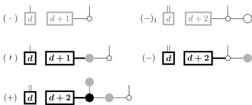
Figure 11. Effect of eliminating simple subschemes

Proof.

This is direct computation, following [Nak07, Sec.2]. ∎

Notation 4.4.

In Fig. 11, the rectangle with label “$d$” denotes an irreducible component $E_{i}$ of $E$ with $E_{i}^{2}=-d$. The small nodes are ${\mathbb{P}}^{1}$’s of square $(-1)$, the large ones of square $(-2)$. Rectangles and nodes are shown in bold black, resp. gray or white, if they appear in $E_{M}$ with multiplicity $2$, resp. $1$ or $0$. The half-edges denote $\operatorname{mult}_{P}(\Delta\cap E_{i})$, which are 2 (double line) or 1 (single line). When we are working with a geometric triple $(X,B+\frac{1+\epsilon}{2}D)$, where $D\in|-2K_{S}-E|$ is a section, these half edges are the local intersection numbers $DE_{i}$ at a point $P\in D\cap E_{i}$. The double edge means that $D$ is tangent to $E_{i}$ at $P$.

The following lemma is a direct consequence of a proof from [Nak07].

Lemma 4.5.

The pair $(S,B)$ is log canonical iff for every irreducible component $E_{i}$ of $E$ in the fundamental triplet $(X,E,\Delta)$, one has $\operatorname{mult}_{E}(E_{i})\leq 2$, $\Delta$ is disjoint from the nodes of the double part $\llcorner E\lrcorner$ of $E$, and $\operatorname{mult}_{P}(\Delta\cap E_{i})\leq 2$ for every irreducible component $E_{i}$ with $\operatorname{mult}_{E}(E_{i})=~{}2$ and all $P\in\Delta$.

Proof.

Follows immediately from the proof of [Nak07, Cor. 4.7].∎

Theorem 4.6.

Let $(M,E_{M})$ be a basic pair with $M$ the minimal resolution of singularities of a strictly log canonical log del Pezzo surface with boundary $(S,B)$ of index $\leq 2$ with integral $B$, and let $\phi\colon M\to X$ be a contraction to a minimal basic pair so that $(M,E_{M})$ is obtained from a quasi fundamental triplet $(X,E,\Delta)$ by eliminating the 0-dimensional scheme $\Delta$. Then

1. If a component $E_{i}$ of $E$ has multiplicity 1 then its strict preimage on $M$ must be isomorphic to ${\mathbb{P}}^{1}$ and have $E_{i}^{2}\leq-2$.

2. Additionally, assume that $\Delta$ is disjoint from the singular part of $E_{\rm red}$ and that for every irreducible component $E_{i}$ of $E$ with $\operatorname{mult}_{E}(E_{i})=1$, one has $\operatorname{mult}_{P}(\Delta\cap E_{i})\leq 2$. Then the only connected components of $\Delta$ are the five subschemes of Def. 4.2.

Remark 4.7.

Concerning the additional assumptions of (2), we note that they are satisfied for the strictly log canonical fundamental triplets by [Nak07, 4.6]. So we can ignore them in the case $g(S,B)\geq 2$.

Proof.

(1) Our condition for the integrality of $B$ means that all components of $E_{M}$ of multiplicity 1 must be contracted by $\alpha\colon M\to S$. They are all ${\mathbb{P}}^{1}$’s with $E_{i}^{2}\leq-2$.

(2) We then go through the short list of subschemes with $\operatorname{mult}_{P}(\Delta\cap E_{i})\leq 2$, eliminating those that lead to $(-1)$-curves $\Gamma$ with $\operatorname{mult}_{E_{M}}(\Gamma)=1$. For example, the case $\Delta=(x,y)\subset E=(y^{2})$ is eliminated. ∎

Nakayama defined fundamental triplets $(X,E,\Delta)$ (without “quasi”) in order to obtain uniqueness for them, in most cases. We pick a different normalization: we pick $(X,E)$ to correspond to one of the pure shapes and all connected components of $\Delta$ to be of type $(\prime)$.

Theorem 4.8.

Let $(S,B)$ be a log del Pezzo surface with boundary $(S,B)$ of index $\leq 2$ of genus $g(S,B)\geq 2$. Then it is one of the following shapes or is obtained from them by any allowable primings as in Theorem 3.18.

1. ${\widetilde{D}}_{2n}$, $D_{2n}$, $D_{2n-1}^{-}$, $A_{2n-1}$, $A_{2n-2}^{-}$, $\raise 0.65pt\hbox{$\kern-2.0pt\phantom{.}^{-}$}\kern-2.0ptA_{2n-3}^{-}$ for $2n\geq 6$.

2. ${\widetilde{E}}_{7}$, $\raise 0.65pt\hbox{$\kern-2.0pt\phantom{.}^{-}$}\kern-2.0ptE_{7}$, $\raise 0.65pt\hbox{$\kern-2.0pt\phantom{.}^{-}$}\kern-2.0ptE_{6}^{-}$.

3. ${\widetilde{E}}_{8}^{-}$, $\raise 0.65pt\hbox{$\kern-2.0pt\phantom{.}^{-}$}\kern-2.0ptE_{8}^{-}$.

Proof.

We go through the complete list [Nak07, 4.7(2)] of fundamental triplets and see that they are as above.

Case $[n;2,e]_{2}$ for $n\geq 0$, $e\leq\max(4,n+1)$ with $\operatorname{mult}_{\ell}F\leq 2$ for any $\ell\leq F$. This means that $X={\mathbb{F}}_{n}$ and $E=2\sigma+F$, where $F\sim e\ell$ is a sum of several fibers, each with multiplicity $\leq 2$, and $\Delta\cap\sigma=\emptyset$. We have $L\sim 2\sigma_{\infty}+(4-e)\ell$ and $L\sigma=4-e$.

If $e=0$ then $\Delta=\emptyset$. This is ${\widetilde{D}}_{2n+8}$, so we obtain ${\widetilde{D}}_{2m}$ for $2m\geq 8$.

If $e=1$ then we must have $\Delta=(\cdot\cdot)$, that is two disjoint copies of $(\cdot)$ contained in a fiber $F$, or $(-)_{1}$ which is a degeneration of it. Let us use the extended notation $[n;2,0;\cdot\cdot]$, resp. $[n;2,0;-_{1}]$ by writing $\Delta$ at the end. Note that we must apply $(\cdot)$ twice, otherwise ${\widetilde{F}}$ is a $(-1)$-curve in $E_{M}$ with multiplicity 1, which is not allowed by Theorem 4.6.

Contracting one of the $(-1)$-curves back and then $F_{i}$, we can view this as the quasi fundamental triplet $[n-1;2,0;\prime]$, which is ${\widetilde{D}}_{2n+6}^{\prime}$. Thus, we get ${\widetilde{D}}_{2m}^{\prime}$ for $2m\geq 6$.

In the degenerate case $\Delta=(-)_{1}$ of $(\cdot\cdot)$, the direction of the “prime” coincides with the direction of the fiber $\ell$ on ${\mathbb{F}}_{n-1}$ for the triplet $[n-1;2,0;\prime]$. In that case the strict preimage of this fiber gives an extra $(-2)$-curve, and the surface $Y$ acquires an extra $A_{1}$ singularity outside of $B$.

If $e=2$ and $F=\ell_{1}+\ell_{2}$ then we get $[n-2;2,0;{\prime\prime}]$ this way, which is ${\widetilde{D}}_{2n+4}^{{\prime\prime}}$. Since $n\geq 1$, we get ${\widetilde{D}}_{2m}^{{\prime\prime}}$ for $2m\geq 6$. Similarly when $e=3,4$ and $F$ is the sum of $e$ distinct fibers, we get ${\widetilde{D}}_{2m}^{\prime{\prime\prime}}$ and ${\widetilde{D}}_{2m}^{{\prime\prime}{\prime\prime}}$ for $2m\geq 6$. Similar to the above, for every priming the preimage of the corresponding fiber $\ell$ gives an $(-2)$-curve which gives an additional singularity of $Y$.

Now consider the case when $e=2$ and $F=2\ell$ is a double fiber. If $\Delta=\emptyset$ then this is $D_{2n+4}$, i.e. $D_{2m}$ for $2m\geq 6$. For $\Delta=-,\prime,{\prime\prime},+$ we get $D_{2m-1}^{-}$, $D_{2m}^{\prime}$, $D_{2m}^{{\prime\prime}}$, $D_{2m-1}^{+}$ for $2m\geq 6$. Adding single fibers to $F$, i.e. $F=2\ell+\ell_{1}$ or $2\ell+\ell_{1}+\ell_{2}$, gives priming on the left side, which produces all the cases $\kern-2.0pt\phantom{.}^{\prime}\kern-2.0ptD^{?}$ and $\kern-2.0pt\phantom{.}^{\prime\prime}\kern-2.0ptD^{?}$ for $2m\geq 6$.

Finally, $e=4$, $F=2\ell_{1}+2\ell_{2}$ and $\Delta=\emptyset$ gives $A_{2n-1}$. Adding $\Delta=-,\prime,{\prime\prime},+$ adds corresponding decorations in the $A$ case, with each $-,+$ decreasing the index by 1.

Case $[1;2,2]_{2\infty}$: $Y={\mathbb{F}}_{1}$, $E=2\sigma_{\infty}$, and $\Delta=\emptyset$. This is ${\widetilde{D}}_{6}$.

Case $[2]_{2}$ with $\operatorname{mult}_{P}(\Delta\cap\ell)\leq 2$ for any $P\in\ell$: $Y={\mathbb{P}}^{2}$, $E=2\ell$ and $L={\mathcal{O}}(4)$. For $\Delta=\emptyset$, this is ${\widetilde{E}}_{7}$. For $\Delta=(-)$, resp. $(--)$, this is $\raise 0.65pt\hbox{$\kern-2.0pt\phantom{.}^{-}$}\kern-2.0ptE_{7}$, $\raise 0.65pt\hbox{$\kern-2.0pt\phantom{.}^{-}$}\kern-2.0ptE_{6}^{-}$. Considering various other possibilities for $\Delta$ leads to all the allowable primings of ${\widetilde{E}}_{7}$, $\raise 0.65pt\hbox{$\kern-2.0pt\phantom{.}^{-}$}\kern-2.0ptE_{7}$, $\raise 0.65pt\hbox{$\kern-2.0pt\phantom{.}^{-}$}\kern-2.0ptE_{6}^{-}$.

Case $[2;1,2]_{2+}$ with $\operatorname{mult}_{P}(\Delta\cap\ell)\leq 2$ for any $P\in\ell$: $Y={\mathbb{F}}_{2}$, $E=\sigma+2\ell$, $\deg(\Delta\cap\ell)\leq 3$ and $\Delta\cap\sigma=\emptyset$. For $\Delta=\emptyset$ this is ${\widetilde{E}}_{8}^{-}$, and for $\Delta=(-)$ this is $\raise 0.65pt\hbox{$\kern-2.0pt\phantom{.}^{-}$}\kern-2.0ptE_{8}^{-}$. Considering various other possibilities for $\Delta$ leads to all the allowable primings of ${\widetilde{E}}_{8}^{-}$ and $\raise 0.65pt\hbox{$\kern-2.0pt\phantom{.}^{-}$}\kern-2.0ptE_{8}^{-}$.

Case $[0;2,1]_{0}$. This is a typo, this is a klt case so it does not appear. ∎

4C. $K_{M}+L_{M}$ is nef and $g=1$

In this case the main result of [Nak07] is (3.12) which says that $S$ must be a Gorenstein log del Pezzo surface and $2B\sim-K_{S}$. To apply it in our case, we would have to find all Gorenstein del Pezzo surfaces with Du Val singularities and $K_{S}$ divisible by 2 as a Weil divisor – of which there are many – and then consider all the possibilities for $B$.

Instead, we adopt a different strategy. Let us define a weak basic pair with the same definition as a basic pair but dropping the condition $({\mathcal{C}}2)$ that $2g-2>0$. Similarly, we define a weak quasi fundamental triplet $(X,E,\Delta)$ by asking that $X$ in $({\mathcal{F}}1)$ is merely a weak minimal basic pair. Then:

1. It is still true that $K_{M}+L_{M}$ is nef for any weak basic pair obtained by eliminating a 0-dimensional scheme of a weak fundamental triple $(X,E,\Delta)$: the corresponding proofs in [Nak07, 4.2, 3.14 nefness] go through.

2. We have additional conditions $K_{M}+L_{M}=K_{M}+E_{M}=0$ by [Nak07, 3.12].

3. Our Theorem 4.6 still holds.

4. We have to check separately that $L_{M}$ is big, this condition is no longer automatic. However, this is easy to do: $L^{2}/2$ drops by $\deg(\Delta)/2$, i.e. by 1 under the operations $(\prime)$, $(-)_{1}$, $(-)$, and by 2 under $({\prime\prime})$.

Lemma 4.9.

The weak fundamental triplets for strictly lc pairs $(S,B)$ are:

1. $X={\mathbb{P}}^{2}$, $E=2\ell_{1}+\ell_{2}$.

2. $X={\mathbb{F}}_{0}$, and (a) $E=2\sigma+2\ell$, (b) $E=2\sigma+\ell_{1}+\ell_{2}$, (c) $E=2D$, $D\sim\sigma+\ell$.

3. $X={\mathbb{F}}_{1}$, and (a) $E=2\sigma+2\ell_{1}+\ell_{2}$, (b) $E=2\sigma+\ell_{1}+\ell_{2}+\ell_{3}$,
   (c) $E=\sigma+\sigma_{\infty}+2\ell$, (d) $E=2\sigma_{\infty}+\ell$.

4. $X={\mathbb{F}}_{2}$, and (a) $E=2\sigma+2\ell_{1}+2\ell_{2}$, (b) $E=2\sigma+2\ell_{1}+\ell_{2}+\ell_{3}$,
   (c) $E=2\sigma+\ell_{1}+\ell_{2}+\ell_{3}+\ell_{4}$, (d) $E=\sigma+2\ell+\sigma_{\infty}$, (e) $E=2\sigma_{\infty}$.

Proof.

Immediate: $X={\mathbb{P}}^{2}$ or ${\mathbb{F}}_{n}$, $L=-K_{X}$ must be nef, and $E=-2K_{X}-L$ must have at least one component of multiplicity 2. We simply list the possibilities. ∎

Theorem 4.10.

Let $(S,B)$ be a log del Pezzo surface with boundary $(S,B)$ of index $\leq 2$ of genus $g(S,B)=1$. Then it is one of one of the shapes ${\widetilde{D}}_{4}$, $D_{4}$, $A_{3}$, $A_{2}^{-}$, $\raise 0.65pt\hbox{$\kern-2.0pt\phantom{.}^{-}$}\kern-2.0ptA_{1}^{-}$, or is obtained from one of them by any allowable primings as in Theorem 3.18.

Proof.

The pairs of Lemma 4.9 in which all components of $E$ have multiplicity 2 already appear in our classification: (2a) $D_{4}$, (2c) ${\widetilde{D}}_{4}$, (4a) $A_{3}$, (4e) degenerate case of ${\widetilde{D}}_{4}$. Our first step is to reduce all other cases to them.

Let us begin with case (1). The line $\ell_{2}$ must be blown up at least once by Theorem 4.6(1). Thus, we are reduced to case (2).

Now consider for example case (2b). The fiber $\ell_{1}$ must be blown up at least once, again by (4.6)(1). Let $\tau\colon X^{\prime}\to X$ be the first blowup at a point $P\in E$ and let $E_{0}$ be the exceptional $(-1)$-curve. We have $K_{X^{\prime}}+E^{\prime}=\tau^{*}(K_{X}+E)=0$. If $P=\ell_{1}\cap\sigma$ then $E_{0}$ appears in $E^{\prime}$ with coefficient 2, otherwise it appears with coefficient 0; either way it is even. Let $X^{\prime}\to X^{\prime\prime}$ be the contraction of the strict preimage of $\ell_{1}$, which is a $(-1)$-curve on $X^{\prime}$. We obtain another minimal model $M\to X^{\prime\prime}$ for $M$ which has fewer components of multiplicity 1 in $E$.

This way, we reduce all cases to the purely even cases above except cases (3c) and (4d). Consider now (3c). The curve $\sigma_{\infty}$ has to be blown up at least once. Blowing up and contracting the strict preimage of a fiber reduces to the case (3a) which was already considered. The case (4d) reduces to (3c) and then to (3a).

So now we are reduced to the pairs of shapes $D_{4}$, $A_{3}$, ${\widetilde{D}}_{4}$ and the pairs obtained from them by eliminating 0-dimensional subschemes $\Delta$. The conditions of Theorem 4.6(2) hold, so the connected components of $\Delta$ have types $(\prime)$, $(-)$, $(+)$. In the cases $D_{4}$, $A_{3}$ we also have $\deg(\Delta\cap E_{i})\leq 2$ for $i=1,2$. In all three cases, $\deg(\Delta)\leq 6$ by the condition $L_{M}^{2}>0$.

So let us now begin with $D_{4}$ and consider different possibilities for $\Delta$. If one or two components of $\Delta$ are $(-)$ then we get respectively $D_{3}^{-}=A_{3}^{\prime}$ and $\raise 0.65pt\hbox{$\kern-2.0pt\phantom{.}^{-}$}\kern-2.0ptD_{2}^{-}=\raise 0.65pt\hbox{$\kern-2.0pt\phantom{.}^{-}$}\kern-2.0ptA_{2}^{\prime}$. If the components are $(+)$ then we get respectively $D_{3}^{+}=A_{3}^{{\prime\prime}}$ and $\raise 0.65pt\hbox{$\kern-2.0pt\phantom{.}^{-}$}\kern-2.0ptD_{2}^{+}=\kern-2.0pt\phantom{.}^{\prime\prime}\kern-2.0ptA_{3}^{-}$. When the components of $\Delta$ are $(\prime)$, we get the usual primings.

For ${\widetilde{D}}_{4}$, $\Delta=(-)$ gives $D_{4}^{\prime}$ and $\Delta=(--)$ gives $\kern-2.0pt\phantom{.}^{\prime}\kern-2.0ptA_{3}^{\prime}$, with other combinations of $(-)$, $(+)$, $(\prime)$ giving primings of those. For $A_{3}$, it is easier: $\Delta=(-)$, $(-,-)$, $(+)$ etc. gives the usual $A_{2}^{-}$, $\raise 0.65pt\hbox{$\kern-2.0pt\phantom{.}^{-}$}\kern-2.0ptA_{1}^{-}$, $A_{2}^{+}$ and adding $(\prime)$’s gives the usual primings. ∎

This completes the proof of Theorem A. We now switch back from the notation of [Nak07] to our notation $\pi\colon(X,D+\epsilon R)\to(Y,C+\frac{1+\epsilon}{2}B)$.

5. Moduli of $ADE$ pairs

5A. Two-dimensional projections of $ADE$ lattices

Here, we fix the notations from representation theory and prove a number of basic results that will be used in the remainder of the paper.

Notation 5.1.

$\Lambda$ will denote one of the root lattices $A_{n}$, $D_{n}$, $E_{n}$, and $\Lambda^{*}\supset\Lambda$ its dual, the weight lattice. One has $\Lambda^{*}=\oplus_{i=1}^{n}{\mathbb{Z}}\alpha_{i}$ and $\Lambda^{*}=\oplus_{i=1}^{n}{\mathbb{Z}}\varpi_{i}$, where $\alpha_{i}$ are the simple roots and $\varpi_{i}$ the fundamental weights (same as fundamental coweights). One has $\langle\alpha_{i},\varpi_{j}\rangle=\sigma_{ij}$.

Notation 5.2.

We label the nodes of the Dynkin diagrams as in Figs. 1, 2, 3. For example, for the $E_{8}$ diagram we denote the nodes by $p^{\prime\prime}$, $p^{\prime}_{1}$, $p^{\prime}_{2}$, $p_{0},\dotsc,p_{4}$. For the $D_{n}$ diagram they are $p^{\prime\prime}$, $p^{\prime}_{1}=p^{\prime}$, $p_{0},\dotsc,p_{n-3}$. We use the same notation to denote the roots and fundamental weights, i.e. we call them $\alpha^{\prime\prime}$, $\alpha^{\prime}_{1}=\alpha^{\prime}$, etc.

In addition, for each of the polytopes $P$ in Figs. 1, 2, 3 we have the special vertex $p_{*}$ and two vertices $p_{\ell},p_{r}$ which are the end points of the left and right sides. For example, for the $E_{8}$ diagram one has $p_{\ell}=p^{\prime}_{3}$ and $p_{r}=p_{5}$, and for $D_{n}$ they are $p_{\ell}=p^{\prime}_{2}$ and $p_{r}=p_{n-2}$.

Definition 5.3.

We define the extended weight lattice as $\Lambda^{*}\oplus{\mathbb{Z}}^{2}$, and we denote the basis of ${\mathbb{Z}}^{2}$ by $\{\varpi_{l},\varpi_{r}\}$.

Lemma 5.4.

For pure $ADE$ shapes, the rule $\varpi_{i}\mapsto p_{i}-p_{*}$ defines a homomorphism

$$\phi\colon\Lambda^{*}\oplus{\mathbb{Z}}\varpi_{\ell}\oplus{\mathbb{Z}}\varpi_{r}\xrightarrow{\phi}{\mathbb{Z}}^{2}.$$

The projection $\pi_{1}\colon\Lambda^{*}\oplus{\mathbb{Z}}\varpi_{\ell}\oplus{\mathbb{Z}}\varpi_{r}\to\Lambda^{*}$ identifies $\ker\phi$ with $\Lambda$. The homomorphism $\phi$ is surjective for $D,E$ shapes, and one has $\operatorname{coker}\phi={\mathbb{Z}}_{2}$ for $A$ shapes.

Proof.

Any root $\alpha$ can be expressed as $\alpha=\sum_{\varpi}\langle\alpha,\varpi\rangle$ with the sum going over the $n$ fundamental weights $\varpi$. In particular, if $p_{i-1}$, $p_{i}$, $p_{i+1}$ are three consecutive nodes in a chain then

(5.1) $$\alpha_{i}=2\varpi_{i}-\varpi_{i-1}-\varpi_{i+1}\xrightarrow{\phi}2p_{i}-p_{i-1}-p_{i+1}=0$$

For an end node $p_{i}$ next to $p_{r}$ one has

(5.2) $$\alpha_{i}-\varpi_{r}=2\varpi_{i}-\varpi_{i-1}-\varpi_{r}\xrightarrow{\phi}2p_{i}-p_{i-1}-p_{r}=0$$

and similarly for the node next to $p_{\ell}$. For a node $p_{0}$ occurring at a corner of the polytope, one has

(5.3) $$\alpha_{0}=2\varpi_{0}-\varpi_{1}-\varpi_{1}^{\prime}-\varpi^{\prime\prime}\xrightarrow{\phi}2p_{0}-p_{1}-p_{1}^{\prime}-p^{\prime\prime}+p_{*}=0$$

Thus, $\Lambda=\langle\alpha\rangle\subset\ker\phi$, and it is easy to see that the equality holds. ∎

Recall that the finite group $\Lambda^{*}/\Lambda$ is ${\mathbb{Z}}_{n+1}$ for $A_{n}$, ${\mathbb{Z}}_{2}^{2}$ for $D_{2n}$, ${\mathbb{Z}}_{4}$ for $D_{2n-1}$, and ${\mathbb{Z}}_{3}$, ${\mathbb{Z}}_{2}$, $0$ for $E_{6}$, $E_{7}$, $E_{8}$ respectively.

Corollary 5.5.

${\mathbb{Z}}^{2}/\langle p_{\ell}-p_{*},p_{r}-p_{*}\rangle$ is equal to $\Lambda^{*}/\Lambda$ for the pure $D$ and $E$ shapes, and $(\Lambda^{*}/\Lambda)\oplus{\mathbb{Z}}_{2}$ for the pure $A$ shapes.

Lemma 5.6.

For primed $ADE$ shapes which admit a toric description (see Subsection 3D) the rule $\varpi\mapsto p-p_{*}$ defines a homomorphism $\phi\colon\Lambda^{*}\oplus{\mathbb{Z}}\varpi_{\ell}\oplus{\mathbb{Z}}\varpi_{r}\xrightarrow{\phi}{\mathbb{Z}}^{2}.$ The projection $\pi_{1}\colon\Lambda^{*}\oplus{\mathbb{Z}}\varpi_{\ell}\oplus{\mathbb{Z}}\varpi_{r}\to\Lambda^{*}$ identifies $\ker\phi$ with $\Lambda\subset\Lambda^{\prime}\subset\Lambda^{*}$ given below

$$\begin{array}[h]{lll}\text{shape}&\Lambda^{\prime}/\Lambda&\text{generators}\\ \hline\cr\kern-2.0pt\phantom{.}^{\prime}\kern-2.0pt\kern-1.0ptA_{2n-1},\kern-2.0pt\phantom{.}^{\prime}\kern-2.0pt\kern-1.0ptA_{2n-2}^{-}&0&\\ \kern-2.0pt\phantom{.}^{\prime}\kern-2.0pt\kern-1.0ptA_{2n-1}^{\prime}&{\mathbb{Z}}_{2}&\varpi_{n}\\ D_{2n}^{\prime}\text{ for }n\text{ even, resp. odd}&{\mathbb{Z}}_{2}&\varpi^{\prime}\text{ resp. }\varpi^{\prime\prime}\end{array}$$

Proof.

For the corner node $p_{0}$ in $\kern-2.0pt\phantom{.}^{\prime}\kern-2.0pt\kern-1.0ptA_{2n-1},\kern-2.0pt\phantom{.}^{\prime}\kern-2.0pt\kern-1.0ptA^{-}_{2n-2}$ one uses the corner relation (5.3) with $\varpi^{\prime}$ replaced by $\varpi_{\ell}$, and similarly for $D^{\prime}_{2n}$. Additionally: for $\kern-2.0pt\phantom{.}^{\prime}\kern-2.0pt\kern-1.0ptA^{\prime}_{2n-1}$ one has $\varpi_{n}-\varpi_{\ell}-\varpi_{r}\xrightarrow{\phi}0$, and for $D_{2n}$ one has $\phi(\varpi_{r}+\lfloor\frac{n}{2}\rfloor\varpi_{\ell})=\phi(\varpi^{\prime})$, resp. $=\phi(\varpi^{\prime\prime})$. See Fig. 8 for the node notations. ∎

5B. Moduli of $ADE$ pairs of pure shapes

In this subsection we prove the first part of Theorem B. Recall that in Section 3 we associated to each $ADE$ pair $(Y,C+\frac{1+\epsilon}{2}B)$ an $ADE$ root lattice. We use the notation introduced in Section 5A.

Definition 5.7.

We define the tori $T_{\Lambda}=\operatorname{Hom}(\Lambda,{\mathbb{C}}^{*})$ and $T_{\Lambda^{*}}=\operatorname{Hom}(\Lambda^{*},{\mathbb{C}}^{*})$ both isomorphic to $({\mathbb{C}}^{*})^{n}$. We also define a finite multiplicative group $\mu_{\Lambda}=\operatorname{Hom}(\Lambda^{*}/\Lambda,{\mathbb{C}}^{*})$. Thus, $\mu_{\Lambda}=\mu_{n+1}$ for $A_{n}$, $\mu_{2}^{2}$ for $D_{2n}$, $\mu_{4}$ for $D_{2n-1}$, and it is $\mu_{3}$, $\mu_{2}$, $1$ for $E_{6}$, $E_{7}$, $E_{8}$ respectively.

Warning 5.8.

The theorem below is for pairs in which we distinguish the two sides $C_{1}$ and $C_{2}$. The moduli stack for the pairs with a single $C$ is the ${\mathbb{Z}}_{2}$-quotient for the shapes with the left / right symmetry, and is the same for the nonsymmetric shapes.

Theorem 5.9.

The moduli stack of $ADE$ pairs of a fixed pure $ADE$ shape is

$$[\operatorname{Hom}(\Lambda^{*},{\mathbb{C}}):\mu_{\Lambda}\times\mu_{2}]=[T_{\Lambda}:W_{\Lambda}\times\mu_{2}] A$$ for shapes

$$[\operatorname{Hom}(\Lambda^{*},{\mathbb{C}}):\mu_{\Lambda}]=[T_{\Lambda}:W_{\Lambda}] D E$$ for and shapes.

Remark 5.10.

The first presentation is convenient for finding automorphism groups. In particular, the maximal automorphism group that a pair can have is $\mu_{\Lambda}\times\mu_{2}$ for $A$ shapes and $\mu_{\Lambda}$ for $D$ and $E$ shapes. The second form is convenient for compactifications, which in Section 6 are shown to be quotients of toric varieties by Weyl groups.

Proof.

We first note that the pair $(Y,C+\frac{1+\epsilon}{2}B)$ is log canonical near the boundary $C$ iff the divisor $B$ intersects $C$ transversally. Vice versa, with this condition satisfied the pair $(Y,C+\frac{1+\epsilon}{2}B)$ for $0<\epsilon\ll 1$ is automatically log canonical. Otherwise, the pair $(Y,C+\frac{1}{2}B)$ is not log canonical. But by [Sho92, 6.9] the non-klt locus must be connected, with a single exception when it may have two components, both of them simple, i.e. on a resolution each should give a unique curve with discrepancy $-1$. For an $ADE$ surface the curve $C=C_{1}+C_{2}$ is connected with two irreducible components, so they are not simple. (We thank V.V. Shokurov for this argument.)

Each of the $ADE$ shapes is toric, and the polarized toric variety $(Y,L)$ corresponds to a lattice polytope $P$ as in Figs. 1, 2, 3. However, $C=C_{1}+C_{2}$ gives only part of the toric boundary. Fixing the torus structure is equivalent to making a choice for the remainder of the torus boundary: one curve for the $A$ shapes and two curves for the $D,E$ shapes. With this choice made $(Y,L)$ is a polarized toric surface, and the equation of $B$ is $f\in H^{0}(Y,L)=\oplus_{m\in{\mathbb{Z}}^{2}\cap P}\,{\mathbb{C}}e^{m},\ \text{where }e^{(k,l)}=x^{k}y^{l}.$

For the $A$ shapes the remaining toric boundary has the equation $y^{2}\in H^{0}(Y,L)$. All the other choices for the toric boundary differ by the transformation $y\mapsto y+a(x)$. Completing the square we can make the coefficients of the monomials $yx^{i}$ in $f$ all zero. By rescaling $x\mapsto\alpha x$, $y\mapsto\beta y$ we can put the equation $f$ in the form given in Table 5. In this table, $A_{n}^{?}$ denotes either $A_{n}$ or $A_{n}^{-}$ depending on the parity of $n$, and similarly for $D,E$.

$$\begin{array}[]{cll}\text{shape}&f_{\rm bdry}&f_{\rm dyn}\\ \hline\cr A_{n}^{?}&y^{2}+1+x^{n+1}&c_{1}x+\dotsc+c_{n}x^{n}\\ \raise 0.65pt\hbox{$\kern-2.0pt\phantom{.}^{-}$}\kern-4.0ptA_{n}^{?}&y^{2}+x(1+x^{n+1})&x(c_{2}x+\dotsc+c_{n+1}x^{n})\\ D_{n}^{?}&x^{2}y^{2}+y^{2}+x^{n-2}&c^{\prime\prime}xy+c^{\prime}_{1}y+c_{0}+c_{1}x+\dotsc+c_{n-3}x^{n-3}\\ \raise 0.65pt\hbox{$\kern-2.0pt\phantom{.}^{-}$}\kern-2.0ptE_{n}^{?}&x^{2}y^{2}+y^{3}+x^{n-3}&c^{\prime\prime}xy+c^{\prime}_{1}y+c^{\prime}_{2}y^{2}+c_{0}+c_{1}x+\dotsc+c_{n-4}x^{n-4}\\ \hline\cr\end{array}$$

Table 5. Normal forms for the equation $f=f_{\rm bdry}+f_{\rm dyn}$ of divisor $B$

For the $D$ and $E$ shapes the remaining toric boundary has the equation $(xy)^{2}\in H^{0}(Y,L)$. All other choices for the toric boundary differ by the transformations $x\mapsto x+a$, $y\mapsto y+b(x)$, with $\deg b(x)\leq\frac{1}{2}(n-3)$ for $D_{n}$ and $\deg b(x)\leq\frac{1}{2}(n-4)$ for $E_{n}$; and then rescaling $x$ and $y$. Using such transformations, one can put the equation $f$ in the form given in Table 5 in an essentially unique way .

The only remaining choice is the normalization of $f_{\rm bdry}$, which is unique up to the action of $\operatorname{Hom}({\mathbb{Z}}^{2}/\langle p_{\ell}-p_{*},p_{r}-p_{*}\rangle,{\mathbb{C}}^{*})$, equal to $\mu_{\Lambda}$ by Corollary 5.5. The end result is a normal form, given in Table 5, which is unique up to $\mu_{\Lambda}$. This gives the stack $[{\mathbb{A}}^{n}:\mu_{\Lambda}]$. Finally, in the $A$ shapes every pair has an additional $\mu_{2}$ automorphism $y\mapsto-y$. This gives the first presentation of the moduli stack, as a $\mu_{\Lambda}\times\mu_{2}$, resp. $\mu_{\Lambda}$ quotient of ${\mathbb{A}}^{n}$.

It is a well known and easy to prove fact that the ring of invariants ${\mathbb{C}}[\Lambda^{*}]^{W_{\Lambda}}$ is the polynomial ring ${\mathbb{C}}[\chi_{1},\dotsc,\chi_{n}]$, where $\chi_{i}=\chi(\varpi_{i})$ are the characters of the fundamental weights ([Bou05, Ch.8, §7, Thm.2]). In other words, $T_{\Lambda^{*}}/W_{\Lambda}={\mathbb{A}}^{n}$, with the coordinates $\chi_{i}$. The $\mu_{\Lambda}$-actions on $T_{\Lambda^{*}}$ and ${\mathbb{A}}^{n}$ are given by the compatible $(\Lambda^{*}/\Lambda)$-gradings; thus they commute with the $W$-action. The $\mu_{\Lambda}$ action on $T_{\Lambda^{*}}$ is free, and $T_{\Lambda^{*}}/\mu_{\Lambda}=T_{\Lambda}$. Thus

$$[{\mathbb{A}}^{n}:\mu_{\Lambda}]=[(T_{\Lambda^{*}}:W):\mu_{\Lambda}]=[(T_{\Lambda^{*}}:\mu_{\Lambda}):W]=[T_{\Lambda}:W],$$

giving the second presentation. For the $A$ shapes the additional $\mu_{2}$ action commutes with both $\mu_{\Lambda}$ and $W$. ∎

5C. Moduli of $ADE$ pairs of toric primed shapes

We state the theorem analogous to Theorem 5.9 for the primed $ADE$ shapes which admit a toric description (see Section 3D). It can be proved analogously to the theorem above, using Lemma 5.6, or can be seen as an immediate consequence of Theorem 5.12.

Theorem 5.11.

The moduli stack of $ADE$ pairs of a fixed toric primed shape is

$$[\operatorname{Hom}(\Lambda^{*},{\mathbb{C}}):\mu_{\Lambda^{\prime}}]=[T_{\Lambda^{\prime}}:W_{\Lambda}],\quad\text{where }T_{\Lambda^{\prime}}=\operatorname{Hom}(\Lambda^{\prime},{\mathbb{C}}^{*}),$$

$\mu_{\Lambda^{\prime}}=\operatorname{Hom}(\Lambda^{*}/\Lambda^{\prime},{\mathbb{C}}^{*})$, and the lattice $\Lambda\subset\Lambda^{\prime}\subset\Lambda^{*}$ is given in Lemma 5.6.

5D. Moduli of $ADE$ pairs of all primed shapes

In this subsection we find the moduli stack for all primed shapes, including those which do not admit a toric description, and in doing so complete the proof of Theorem B. We still mark the sides as left and right, even if some or all of the boundary curves are contracted.

Theorem 5.12.

The moduli stack of pairs of a fixed primed shape is

$$[\operatorname{Hom}(\Lambda^{*},{\mathbb{C}}):\mu_{\Lambda^{\prime}}\times W_{0}]=[T_{\Lambda^{\prime}}:W_{\Lambda}\rtimes W_{0}],$$

where $\mu_{\Lambda^{\prime}}=\operatorname{Hom}(\Lambda^{*}/\Lambda^{\prime},{\mathbb{C}}^{*})$ and the lattice $\Lambda\subset\Lambda^{\prime}\subset\Lambda^{*}$ is as follows:

$$\begin{array}[h]{lll}\text{shape}&\Lambda^{\prime}/\Lambda&\text{generators}\\ \hline\cr\kern-2.0pt\phantom{.}^{\prime}\kern-2.0pt\kern-1.0ptA_{2n-1},\kern-2.0pt\phantom{.}^{\prime}\kern-2.0pt\kern-1.0ptA_{2n-2}^{-}&0&\\ \kern-2.0pt\phantom{.}^{\prime}\kern-2.0pt\kern-1.0ptA_{2n-1}^{\prime}&{\mathbb{Z}}_{2}&\varpi_{n}\\ D_{2n}^{\prime}\text{ for }n\text{ even, resp. odd}&{\mathbb{Z}}_{2}&\varpi^{\prime}\text{ resp. }\varpi^{\prime\prime}\\ \kern-2.0pt\phantom{.}^{\prime}\kern-2.0ptD_{2n},\text{ resp. }\kern-2.0pt\phantom{.}^{\prime}\kern-2.0ptD_{2n-1}^{-}&{\mathbb{Z}}_{2}&\varpi_{2n-3},\text{ resp. }\varpi_{2n-4}\\ \kern-2.0pt\phantom{.}^{\prime}\kern-2.0ptD_{2n}^{\prime}\text{ for }n\text{ even, resp. odd}&{\mathbb{Z}}_{2}\times{\mathbb{Z}}_{2}&\varpi_{2n-3},\varpi^{\prime},\text{ resp. }\varpi_{2n-3},\varpi^{\prime\prime}\\ \raise 0.65pt\hbox{$\kern-2.0pt\phantom{.}^{-}$}\kern-2.0ptE^{\prime}_{7}&{\mathbb{Z}}_{2}&\varpi_{3}\end{array}$$

For shapes $\kern-2.0pt\phantom{.}^{\prime\prime}\kern-2.0ptS$ and $S^{\prime\prime}$ the lattices $\Lambda^{\prime}$ are the same as for the unprimed shape $S$, and similarly for $\raise 0.65pt\hbox{$\kern-2.0pt\phantom{.}^{+}$}\kern-2.0ptS$ resp. $S^{+}$ and the unprimed shapes $\raise 0.65pt\hbox{$\kern-2.0pt\phantom{.}^{-}$}\kern-2.0ptS$ resp. $S^{-}$. The additional Weyl group $W_{0}$ is the one given in Theorem 3.32, and its action is described in Theorem 5.13.

Proof.

The pair $({\overline{Y}}^{\prime},{\overline{C}}^{\prime}_{1}+{\overline{C}}^{\prime}_{2}+\frac{1+\epsilon}{2}{\overline{B}}^{\prime})$ is obtained from a pair $(Y,C_{1}+C_{2}+\frac{1+\epsilon}{2}B)$ of pure shape by blowing up several points $P_{i}\in B\cap C$ at the ideals $I_{i}$ with directions equal to the tangent directions of $B$, and then contracting by the semiample line bundle $L^{\prime}$. This construction works for the entire family over ${\mathbb{A}}^{n}=\operatorname{Hom}(\Lambda^{*},{\mathbb{C}})$: we blow up sections and it is easy to see that the sheaf ${\mathcal{L}}^{\prime}$ in the family is relatively semiample.

When priming on a short side, or priming twice on a long side, there are no choices for $\prod I_{i}$. The only 2:1 choice is when there is a long side $C_{s}$ and we prime only at one of the two points in $B\cap C_{s}$. Secondly, as stated in Theorem 3.32, for some shapes of genus 1 there is more than one precursor. These choices define an additional quotient by $W_{0}$. ∎

5E. Definitions of the naive $ADE$ families

For the toric $ADE$ shapes $A$, $\kern-2.0pt\phantom{.}^{\prime}\kern-2.0pt\kern-1.0ptA$, $D$ and $E$ we define explicit modular families of $ADE$ pairs over the torus $T_{\Lambda^{*}}$. We call these the naive families. Blowing up the sections corresponding to the points in $C\cap B$, we obtain the naive families for all the primed $ADE$ shapes.

For the $A_{n}^{?}$-shapes, where $A_{n}^{?}$ is either $A_{n}$ or $A_{n}^{-}$ depending upon the parity of $n$, we take the equation of Table 5 with $c_{i}=\chi_{i}=\chi(\varpi_{i})$, the characters of the fundamental weights, and with $y^{2}$ rescaled to $-(\frac{y}{2})^{2}$, which will be convenient when we come to discuss degenerations.

We recall that the $A_{n}$ root lattice is $\langle e_{i}-e_{j}\rangle\subset{\mathbb{Z}}^{n+1}$ and the dual weight lattice is $A_{n}^{*}=\langle f_{i}\rangle$, where $f_{i}=e_{i}-p$, $p=\frac{1}{n+1}\sum e_{i}$, so that $\sum_{i=1}^{n+1}f_{i}=0$. Thus, ${\mathbb{C}}[\Lambda^{*}]={\mathbb{C}}[t_{1}^{\pm},\dots,t_{n+1}^{\pm}]/(\prod t_{k}-1)$ and ${\mathbb{C}}[\Lambda]={\mathbb{C}}[t_{i}/t_{j}]$, with $t_{i}=e^{f_{i}}$. The first torus is $T_{\Lambda^{*}}=\{\prod t_{i}=1\}\subset({\mathbb{C}}^{*})^{n+1}$, and the second one is $T_{\Lambda}=({\mathbb{C}}^{*})^{n+1}/\operatorname{diag}{\mathbb{C}}^{*}$. One has $T_{\Lambda}=T_{\Lambda^{*}}/\mu_{n+1}$.

The Weyl group is $S_{n+1}$, and the characters of the fundamental weights are the symmetric polynomials $\chi_{i}=\sigma_{i}(t_{k})$. Therefore, the defining equation of the naive family is

(5.4) $$A_{n}^{?}:\ f=-\left(\frac{y}{2}\right)^{2}+\prod_{i=1}^{n+1}(x+t_{i})=-\left(\frac{y}{2}\right)^{2}+1+\chi_{1}x+\dotsc\chi_{n}x^{n}+x^{n+1}.$$

For $\raise 0.65pt\hbox{$\kern-2.0pt\phantom{.}^{-}$}\kern-4.0ptA_{n}^{?}$ shapes we number the nodes $2,\dotsc,n+1$ (cf. Fig. 1) and the equation is as follows, where $\chi_{k}=\sigma_{i-1}(t_{i})$:

(5.5) $$\raise 0.65pt\hbox{$\kern-2.0pt\phantom{.}^{-}$}\kern-4.0ptA_{n}^{?}:f=-\left(\frac{y}{2}\right)^{2}+x\prod_{i=1}^{n+1}(x+t_{i})=-\left(\frac{y}{2}\right)^{2}+x\left(1+\chi_{2}x+\dotsc\chi_{n+1}x^{n}+x^{n+1}\right).$$

For the toric shapes with one corner, i.e. $D_{n}^{?}$, $\raise 0.65pt\hbox{$\kern-2.0pt\phantom{.}^{-}$}\kern-2.0ptE_{n}^{?}$ and $\kern-2.0pt\phantom{.}^{\prime}\kern-2.0pt\kern-1.0ptA_{n}^{?}$ (here again the $?$ is either no decoration or a $-$, depending upon the parity), we make the following change of coordinates. We begin with the affine equation of a double cover $X\to Y$ of the form

$$F(x,y,z)=-xyz+z^{2}+c^{\prime\prime}z+p(x)+q(y)=0.$$

Introducing the variable $w=z-\frac{1}{2}(xy-c^{\prime\prime})$, the equation becomes

$$w^{2}+f(x,y)=0,\qquad f(x,y)=-\left(\frac{xy-c^{\prime\prime}}{2}\right)^{2}+p(x)+q(y)$$

with the same $p(x)$, $q(y)$. Thus, the affine equation of the branch curve $B$ is $f(x,y)$, which we accept as our main equation. Explicitly, the families are:

(5.6) $$\kern-2.0pt\phantom{.}^{\prime}\kern-2.0pt\kern-1.0ptA_{n}^{?}: f=-\left(\frac{xy-c^{\prime\prime}}{2}\right)^{2}+y+c_{0}+c_{1}x+\dotsb+c_{n-2}x^{n-2}+x^{n-1}$$

(5.7) $$D_{n}^{?}: f=-\left(\frac{xy-c^{\prime\prime}}{2}\right)^{2}+y^{2}+c^{\prime}_{1}y+c_{0}+c_{1}x+\dotsb+c_{n-3}x^{n-3}+x^{n-2}$$

(5.8) $$\raise 0.65pt\hbox{$\kern-2.0pt\phantom{.}^{-}$}\kern-2.0ptE_{n}^{?}: f=-\left(\frac{xy-c^{\prime\prime}}{2}\right)^{2}+y^{3}+c^{\prime}_{2}y^{2}+c^{\prime}_{1}y+c_{0}+\dotsb+c_{n-4}x^{n-4}+x^{n-3}$$

In all of these families we take the coefficients to be $c=\chi(\varpi)$, the fundamental characters, i.e. the characters of the fundamental weights corresponding to the $n$ nodes of the Dynkin diagram, using our Notation 5.2.

5F. Action of the extra Weyl group $W_{0}$

When a pure shaped precursor is not uniquely determined, as in Theorem 3.32, there is an additional Weyl group $W_{0}$ acting on the pure shape moduli torus $T_{\Lambda^{\prime}}$. We divide by it in Theorem 5.12.

Theorem 5.13.

The Weyl group $W_{0}$ of Theorem 3.32 acts on $T_{\Lambda^{\prime}}$ as follows:

1. Genus $>1$. For $\kern-2.0pt\phantom{.}^{\prime}\kern-2.0ptD_{2n}^{?}$ and $\kern-2.0pt\phantom{.}^{\prime}\kern-2.0ptD_{2n-1}^{?}$ shapes, $W_{0}=W(A_{1})=S_{2}$ acts by an automorphism of the $D$-lattice switching the two short legs $p^{\prime}$ and $p^{\prime\prime}$. For $\kern-2.0pt\phantom{.}^{\prime\prime}\kern-2.0ptD_{2n}^{?}$ and $\kern-2.0pt\phantom{.}^{\prime\prime}\kern-2.0ptD_{2n-1}^{?}$ shapes, one has $W_{0}=W(A_{1}^{2})=S_{2}^{2}$. The first $S_{2}$ acts by switching the two short legs $p^{\prime}$ and $p^{\prime\prime}$. The second $S_{2}$ gives an additional $S_{2}$ automorphism of the pair $(Y,C+\frac{1+\epsilon}{2}B)$.

2. Genus 1. For the following shapes the action is as in (1) under the identifications: $\kern-2.0pt\phantom{.}^{\prime}\kern-2.0pt\kern-1.0ptA^{\prime}_{3}=\kern-2.0pt\phantom{.}^{\prime}\kern-2.0ptD^{-}_{3}$, $\kern-2.0pt\phantom{.}^{\prime}\kern-2.0pt\kern-1.0ptA^{\prime\prime}_{3}=\kern-2.0pt\phantom{.}^{\prime\prime}\kern-2.0ptD^{-}_{3}$, $D^{\prime}_{4}=\kern-2.0pt\phantom{.}^{\prime}\kern-2.0ptD_{4}$, $D^{\prime\prime}_{4}=\kern-2.0pt\phantom{.}^{\prime\prime}\kern-2.0ptD_{4}$. For $\kern-2.0pt\phantom{.}^{\prime}\kern-2.0ptD^{\prime}_{4}$ the group $W_{0}=W(A_{2})=S_{3}$ acts by permuting the three legs of the $D_{4}$ diagram. For $\kern-2.0pt\phantom{.}^{\prime}\kern-2.0ptD^{\prime\prime}_{4}$, one has $W_{0}=W(A_{3})=S_{4}=S_{3}\ltimes S_{2}^{2}$. Here, $S_{3}$ acts by permuting the legs and $S_{2}^{2}$ gives an extra automorphism group of the pair $(Y,C+\frac{1+\epsilon}{2}B)$.

Proof.

(1) From the equation (5.7) of the $D$-family we see that the side $C_{1}$ is defined by $(y_{0}:y_{1})=(0:1)$, where $y=\frac{y_{1}}{y_{0}}$. There are two points $x=\pm 2$ on $C_{1}$ at which one can prime. For $x=2$, consider the map $\varphi_{+}\colon y\mapsto\frac{c^{\prime\prime}+c^{\prime}}{x-2}-y$, $x\mapsto x$. It is easy to check that the equation (5.7) maps to the same equation but with $c^{\prime}$ and $c^{\prime\prime}$ switched. The map $\varphi_{+}$ is a rational map for a surface of $D^{?}$ shape but it becomes regular on the blowup, a surface of $\kern-2.0pt\phantom{.}^{\prime}\kern-2.0ptD^{?}$ shape. Similarly, for priming at $x=-2$ the map $\varphi_{-}\colon y\mapsto\frac{c^{\prime\prime}-c^{\prime}}{x+2}+y$ works the same way. The composition $\varphi_{-}\circ\varphi_{+}\colon y\mapsto\frac{c^{\prime\prime}-c^{\prime}}{x+2}+\frac{c^{\prime\prime}+c^{\prime}}{x-2}-y$, $x\mapsto x$ exchanges the two branches of the curve $B$, a two-section of the ${\mathbb{P}}^{1}$-fibration. For surfaces $Y$ of $D^{?}$ and $\kern-2.0pt\phantom{.}^{\prime}\kern-2.0ptD^{?}$ shapes this is a rational involution. It becomes a regular involution of a surface of $\kern-2.0pt\phantom{.}^{\prime\prime}\kern-2.0ptD^{?}$ shape, where $B$ is disconnected from $C_{1}$. Case (2) is checked similarly. ∎

Definition 5.14.

Let $W_{00}\subset W_{0}$ be the subgroup which acts trivially on the the points of $T_{\Lambda^{\prime}}$, giving extra automorphisms of the pairs.

Corollary 5.15.

The group $W_{0}/W_{00}$ acts by diagram automorphisms of the decorated Dynkin diagram, permuting the short legs, all of them white circled vertices: for $\kern-2.0pt\phantom{.}^{\prime}\kern-2.0ptD^{?}_{2n}$, $\kern-2.0pt\phantom{.}^{\prime}\kern-2.0ptD^{?}_{2n-1}$, $\kern-2.0pt\phantom{.}^{\prime\prime}\kern-2.0ptD^{?}_{2n}$, $\kern-2.0pt\phantom{.}^{\prime\prime}\kern-2.0ptD^{?}_{2n-1}$, $\kern-2.0pt\phantom{.}^{\prime}\kern-2.0pt\kern-1.0ptA^{\prime}_{3}$, $\kern-2.0pt\phantom{.}^{\prime}\kern-2.0pt\kern-1.0ptA^{\prime\prime}_{3}$ it is two legs, and for $\kern-2.0pt\phantom{.}^{\prime}\kern-2.0ptD_{4}^{\prime}$, $\kern-2.0pt\phantom{.}^{\prime}\kern-2.0ptD_{4}^{\prime\prime}$ three legs, cf. Fig. 6.

6. Compactifications of moduli of $ADE$ pairs

6A. Stable pairs in general and stable $ADE$ pairs

We recall some standard definitions from the theory of moduli of stable pairs. We note in particular a close relationship between the contents of this subsection and work of Hacking [Hac04a, Hac04b], who studied similar ideas in the context of moduli of plane curves.

Definition 6.1.

A pair $(X,B=\sum b_{i}B_{i})$ consisting of a reduced variety and a ${\mathbb{Q}}$-divisor is semi log canonical (slc) if $X$ is $S_{2}$, has at worst double crossings in codimension 1, and for the normalization $\nu\colon X^{\nu}\to X$ writing

$$\nu^{*}(K_{X}+B)=K_{X^{\nu}}+B^{\nu},$$

the pair $(X^{\nu},B^{\nu})$ is log canonical. Here $B^{\nu}=D+\sum b_{i}\nu^{-1}(B_{i})$ and $D$ is the double locus.

Definition 6.2.

A pair $(X,B)$ consisting of a connected projective variety $X$ and a ${\mathbb{Q}}$-divisor $B$ is stable if

1. $(X,B)$ has slc singularities, in particular $K_{X}+B$ is ${\mathbb{Q}}$-Cartier.

2. The ${\mathbb{Q}}$-divisor $K_{X}+B$ is ample.

Next we introduce the objects that we are interested in here: We could work equivalently with the pairs $(Y,C+\frac{1+\epsilon}{2}B)$ or with their double covers $(X,D+\epsilon R)$. We choose the former.

Definition 6.3.

For a fixed degree $e\in{\mathbb{N}}$ a fixed rational number $0<\epsilon\leq 1$, a stable del Pezzo pair of type $(e,\epsilon)$ is a pair $(Y,C+\frac{1+\epsilon}{2}B)$ such that

1. $2(K_{X}+C)+B\sim 0$

2. The divisor $B$ is an ample Cartier divisor of degree $B^{2}=e$.

3. $(Y,C+\frac{1+\epsilon}{2}B)$ is stable in the sense of Definition 6.2.

Definition 6.4.

A family of stable del Pezzo pairs of type $(e,\epsilon)$ is a flat morphism $f\colon({\mathcal{Y}},{\mathcal{C}}+\frac{1+\epsilon}{2}{\mathcal{B}})\to S$ such that $(\omega^{\otimes 2}_{{\mathcal{Y}}/S}({\mathcal{C}})^{**}\simeq{\mathcal{O}}_{Y}$ locally on $S$, the divisor ${\mathcal{B}}$ is a relative Cartier divisor, such that every fiber is a stable del Pezzo pair of type $(e,\epsilon)$. We will denote by ${\mathcal{M}}^{\rm slc}_{\rm dp}(e,\epsilon)$ its moduli stack.

Proposition 6.5.

For a fixed degree $e$ there exists an $\epsilon_{0}(e)>0$ such that for any $0<\epsilon\leq\epsilon_{0}$ the moduli stacks ${\mathcal{M}}^{\rm slc}(e,\epsilon_{0})$ and ${\mathcal{M}}^{\rm slc}(e,\epsilon)$ coincide. The stack ${\mathcal{M}}^{\rm slc}(e,\epsilon_{0})$ is a Deligne-Mumford stack of finite type with a coarse moduli space $M^{\rm slc}(e,\epsilon_{0})$ which is a separated algebraic space.

Proof.

For a fixed surface $Y$, there exists an $0<\epsilon_{0}\ll 1$ such that the pair $(Y,C+\frac{1+\epsilon}{2}B)$ is slc iff $B$ does not contain any centers of log canonical singularities of $(Y,C+\frac{1}{2}B)$: images of the divisors with codiscrepancy $b_{i}=1$ on a log resolution of singularities $Z\to Y^{\nu}\to Y$. There are finitely many of such centers. Then for any $\epsilon<\epsilon_{0}$, the pair $(Y,C+\frac{1+\epsilon_{0}}{2}B)$ is slc iff $(Y,C+\frac{1+\epsilon}{2}B)$ is. Now since $B$ is ample Cartier of a fixed degree, the family of the pairs is bounded, and the number $\epsilon_{0}$ with this property can be chosen universally.

We refer to [KSB88, Kol15], [Ale06] for the existence and projectivity of the moduli space of stable pairs $(X,\sum b_{i}B_{i})$. There are complications arising in the construction when some coefficients $b_{i}\leq\frac{1}{2}$ and when the divisor $B$ is not ${\mathbb{Q}}$-Cartier, all of which are not present in this situation. ∎

Definition 6.6.

For a fixed $ADE$ shape, we denote by $M^{\rm slc}_{ADE}$ the closure of the moduli space of $ADE$ pairs of this shape in $M^{\rm slc}_{\rm dP}(e,\epsilon_{0})$ for $e=B^{2}$, with the reduced scheme structure.

In this Section will show that $M^{\rm slc}_{ADE}$ is proper and that in fact the stable limits of $ADE$ pairs are of a very special kind: they are stable $ADE$ pairs. We will also show that the normalization of $M^{\rm slc}_{ADE}$ is an explicit projective toric variety for a generalized Coxeter fan.

Definition 6.7.

A stable $ADE$ pair is a stable del Pezzo pair $(Y,C+\frac{1+\epsilon}{2}B)$ such that its normalization is a union of $ADE$ pairs $\sqcup(Y^{\nu}_{k},C^{\nu}_{k}+\frac{1+\epsilon}{2}B^{\nu}_{k})$.

Theorem 6.8.

For a stable $ADE$ pair the irreducible components are of two kinds:

1. normal, i.e. $\nu\colon Y^{\nu}_{k}\xrightarrow{\sim}Y_{k}$, or

2. folded: the morphism $\nu\colon Y^{\nu}_{k}\to Y_{k}$ is an isomorphism outside of $C_{k}$, and is a double cover ${\mathbb{P}}^{1}\to{\mathbb{P}}^{1}$ on one or two sides $C^{\nu}_{k,s}\to C_{k,s}$, $s=1,2$. In this case, the side $C^{\nu}_{k,s}$ is necessarily a long side of the $ADE$ pair.

Proof.

The normalization of a stable pair is an isomorphism outside of the double locus and is 2:1 on the double locus, so these are the two possibilities. The side must be long because $\nu^{*}B_{k}\cdot C^{\nu}_{k,s}=2B_{k}\cdot C_{k,s}$ is even and $\geq 2$. ∎

Definition 6.9.

We will call the surfaces of type (2) in the above theorem the folded shapes. We denote a fold by adding the $f$ superscript to the corresponding long side, e.g. $A_{2n-1}^{f}$, $\raise 1.17pt\hbox{$\kern-2.0pt\phantom{.}^{f}$}\kern-4.0ptA_{2n-1}^{f}$, $\raise 0.65pt\hbox{$\kern-2.0pt\phantom{.}^{-}$}\kern-4.0ptA_{2n}^{f}$, $\kern-2.0pt\phantom{.}^{\prime}\kern-2.0pt\kern-1.0ptA_{2n-1}^{f}$. We define the decorated Dynkin diagrams for these shapes by double circling the corresponding end (unfilled) node. We do not draw any pictures for these here.

Next, we extend the naive families of $ADE$ pairs, defined in section 5E, to families of stable pairs over a projective toric variety corresponding to the Coxeter fan. We start with the $A_{n}$ case.

6B. Compactifications of the naive families for the $A$ shapes

Recall that $T_{\Lambda^{*}}=\operatorname{Spec}{\mathbb{C}}[\Lambda^{*}]$. We define the following elements of the homogeneous ring ${\mathbb{C}}[\Lambda^{*}][x,y][\xi]$, with the grading defined by $\deg\xi=1$.

Definition 6.10.

In the $A_{n}^{?}$ shape, where the $?$ denotes either no decoration or a $-$ depending upon the parity of $n$, for each node $p_{1},\ldots,p_{n}$ of the Dynkin diagram we introduce a degree 2 element $u_{i}=e^{\varpi_{i}}x^{i}\cdot\xi^{2}$, where $e^{\varpi_{i}}\in{\mathbb{C}}[\Lambda^{*}]$ is the monomial corresponding to the fundamental weight $\varpi_{i}\in\Lambda^{*}$. In addition, we introduce the degree 2 elements $u_{0}=1\cdot\xi^{2}$ and $u_{n+1}=x^{n+1}\cdot\xi^{2}$, corresponding to the left and right nodes $p_{l}=p_{0}$ and $p_{r}=p_{n+1}$, and $u_{*}=y^{2}\cdot\xi^{2}$ corresponding to the vertex $p_{*}$. Similarly, in the $\raise 0.65pt\hbox{$\kern-2.0pt\phantom{.}^{-}$}\kern-4.0ptA_{n}^{?}$ shape we define the elements $u_{1},\dotsc,u_{n+2}$ and $u_{*}$.

Because even the simplest $ADE$ surface of $A^{-}_{0}$-shape is a weighted projective space ${\mathbb{P}}(1,1,2)$, it is convenient to introduce some square roots.

Definition 6.11.

For the even nodes $p_{2i}$ we introduce the degree 1 elements of the ring $R[\xi]$: $v_{2i}=e^{\varpi_{2i}/2}x^{i}\cdot\xi$ and $v_{*}=y\cdot\xi$. Thus, $v_{2i}^{2}=u_{2i}$ and $v_{*}^{2}=u_{*}$.

We recall that in the naive families (5.4), (5.5) we take the coefficients $c_{i}=\chi_{i}$, the fundamental characters. As in Section 5A, let $\alpha_{i}$ be the simple roots.

Definition 6.12.

Set $a_{i}=e^{-\alpha_{i}}$ for all $i$, and for odd indices set $b_{2i+1}=e^{-\alpha_{2i+1}/2}$. Finally, define normalized coefficients $\widehat{c}_{i}=e^{-\varpi_{i}}c_{i}$.

It is well known that for any dominant weight $\lambda\in\Lambda^{*}$ the character $\chi(\lambda)\in{\mathbb{C}}[\Lambda^{*}]$ is a $W_{\Lambda}$-invariant Laurent polynomial whose highest weight is $\lambda$ and the other weights are of the form $\mu=\lambda-\sum n_{i}\alpha_{i}$ for some $n_{i}\geq 0$. Thus, $\widehat{c}_{k}$ are polynomials in $a_{i}$’s, and $\widehat{c}_{k}=1+(\text{higher terms in }a_{i})$.

With these notations, we consider the equation $f$ of the naive family (5.4) to be the following homogeneous degree 2 element in ${\mathbb{C}}[\Lambda^{*}][x,y][\xi]$ (similarly for $\raise 0.65pt\hbox{$\kern-2.0pt\phantom{.}^{-}$}\kern-4.0ptA_{n}^{?}$):

(6.1) $$f=-\left(\frac{v_{*}}{2}\right)^{2}+u_{0}+\widehat{c}_{1}u_{1}+\dotsc+\widehat{c}_{n}u_{n}+u_{n+1}\in{\mathbb{C}}[\Lambda^{*}][x,y]\cdot\xi^{2}$$

For the construction of the family one might as well work with the ring ${\mathbb{C}}[\frac{1}{2}\Lambda^{*}]$ but we will use the minimal choice for clarity.

Definition 6.13.

Let $M$ be the lattice obtained by adjoining to $\Lambda^{*}$ the vectors $\varpi_{2i}/2$ and $\alpha_{2i+1}/2$ for all $i$. Let $M^{+}=M\cap\sum{\mathbb{R}}_{\geq 0}(-\alpha_{i})$ and $R={\mathbb{C}}[M^{+}]$. Thus, $\operatorname{Spec}R$ is a normal affine toric variety which is a $\mu_{2}^{N}$-cover of ${\mathbb{A}}^{n}=\operatorname{Spec}{\mathbb{C}}[a_{i}]$ for some $N$.

Definition 6.14 (Compactified naive families for the $A_{n}^{?}$, $\raise 0.65pt\hbox{$\kern-2.0pt\phantom{.}^{-}$}\kern-4.0ptA_{n}^{?}$ shapes).

Let $S$ be the graded subring of $R[x,y][\xi]$ generated by $v_{2i}$, $u_{2i+1}$, and $v_{*}$. The compactified naive family is ${\mathcal{Y}}:=\operatorname{Proj}S\to\operatorname{Spec}R$ with a relative Cartier divisor ${\mathcal{B}}=(f)$, $f\in H^{0}({\mathcal{O}}(2))$. We note that since the subring $S^{(2)}$ is generated in degree 1, the sheaf ${\mathcal{O}}_{\operatorname{Proj}S}(2)$ is invertible and ample.

Example 6.15.

For the $A_{1}$ shape, the $A_{1}$ root lattice has ${\mathbb{C}}[\Lambda^{*}]={\mathbb{C}}[t_{1}^{\pm},t_{2}^{\pm}]/(t_{1}t_{2}-1)\cong{\mathbb{C}}[t^{\pm}]$, with $t=e^{\alpha_{1}/2}$. The family is $\operatorname{Proj}S\to{\mathbb{A}}^{1}=\operatorname{Spec}{\mathbb{C}}[b_{1}]$, where $S=R[v_{*},v_{0},u_{1},v_{1}]/(v_{0}v_{2}-b_{1}u_{1})$. One has $\chi_{1}=t+t^{-1}=t(1+b_{1}^{2})$, and the equation of the divisor ${\mathcal{B}}$ is

$$f=-\left(\frac{v_{*}}{2}\right)^{2}+v_{0}^{2}+(1+b_{1}^{2})u_{1}+v_{2}^{2}.$$

Setting $b_{1}=0$ gives the degenerate fiber ${\mathbb{P}}(1,1,2)\cup{\mathbb{P}}(1,1,2)$ with the coordinates $v_{*},v_{0},u_{1}$, resp. $v_{*},v_{2},u_{1}$, glued along a ${\mathbb{P}}^{1}$ with the coordinate $u_{1}$. The restriction of $f$ to ${\mathbb{P}}(v_{*},v_{0},u_{1})$ is $v_{*}^{2}+v_{0}^{2}+u_{1}$, and for ${\mathbb{P}}(v_{*},v_{2},u_{1})$ it is $v_{*}^{2}+v_{2}^{2}+u_{1}$. Thus, the degenerate fiber is a union of two $ADE$ pairs $A_{0}^{-}\raise 0.65pt\hbox{$\kern-2.0pt\phantom{.}^{-}$}\kern-4.0ptA_{0}$ glued along a short side.

For the $\raise 0.65pt\hbox{$\kern-2.0pt\phantom{.}^{-}$}\kern-4.0ptA^{-}_{1}$ shape the family is $\operatorname{Proj}S\to{\mathbb{A}}^{1}=\operatorname{Spec}{\mathbb{C}}[a_{1}]$, where $S=R[u_{1},v_{2},u_{3}]/(u_{1}u_{3}-a_{1}v_{2}^{4})$, and the equation of the divisor is

$$f=-\left(\frac{v_{*}}{2}\right)^{2}+u_{1}+(1+a_{2})v_{2}^{2}+u_{2}.$$

Setting $a_{1}=0$ gives the degenerate fiber ${\mathbb{P}}(1,1,2)\cup{\mathbb{P}}(1,1,2)$ with the coordinates $v_{*},v_{2},u_{1}$, resp. $v_{*},v_{2},u_{3}$, which is the union of two $ADE$ pairs $\raise 0.65pt\hbox{$\kern-2.0pt\phantom{.}^{-}$}\kern-4.0ptA_{0}A_{0}^{-}$ glued along a long side, a ${\mathbb{P}}^{1}$ with the coordinate $v_{2}$.

The general case is essentially a generalization of this simple example. The degenerations of pairs for the slightly more complicated $A^{-}_{2}$ shape are illustrated in Fig. 12.

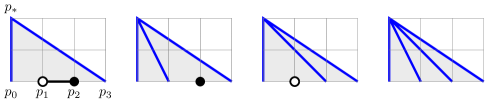
Figure 12. $A_{2}^{-}$ and its degenerations: $A_{0}^{-}\raise 0.65pt\hbox{$\kern-2.0pt\phantom{.}^{-}$}\kern-4.0ptA_{1}^{-}$, $A_{1}A_{0}^{-}$, and $A_{0}^{-}\raise 0.65pt\hbox{$\kern-2.0pt\phantom{.}^{-}$}\kern-4.0ptA_{0}A_{0}^{-}$

Definition 6.16.

The Coxeter fan for a root lattice $\Lambda$ is the fan on $\Lambda_{\mathbb{R}}=\Lambda^{*}_{\mathbb{R}}$ obtained by cutting this vector space by the mirrors $\alpha^{\perp}$ to the roots $\alpha$. Its maximal cones are chambers, the translates of the positive chamber under the action of the Weyl group $W_{\Lambda}$. We denote by $V^{\rm cox}_{M}$ the torus embedding of $T_{M}=\operatorname{Hom}(M,{\mathbb{C}}^{*})$ for the Coxeter fan of $A_{n}$.

Lemma 6.17.

The following relations hold:

1. (Primary) $v_{2i}v_{2i+2}=b_{2i+1}u_{2i+1}$ and $u_{2i-1}u_{2i+1}=a_{2i}v^{4}_{2i}$.

2. (Secondary) $u_{2i-1}u_{2j+1}=v_{2i}^{2}v_{2j}^{2}\cdot A$, $v_{2i-2}u_{2j+1}=v_{2i}v_{2j}^{2}\cdot b_{2i-1}A$, and $v_{2i-2}v_{2j+2}=v_{2i}v_{2j}\cdot b_{2i-1}b_{2j+1}A$, where $A=\prod_{k=2i}^{2j}a_{k}$.

Proof.

An easy direct check using equations (5.1), (5.2). ∎

Theorem 6.18.

The compactified family ${\mathcal{Y}}=\operatorname{Proj}S\to\operatorname{Spec}R$ of shape $A_{n}^{?}$ or $\raise 0.65pt\hbox{$\kern-2.0pt\phantom{.}^{-}$}\kern-4.0ptA_{n}^{?}$ is flat. The degenerate fibers are over the subsets given by setting some $a_{i}$’s to zero. Every fiber of this family is a stable $ADE$ pair which is a union of $ADE$ pairs of shapes obtained by subdividing the $A_{n}^{?}$, resp. $\raise 0.65pt\hbox{$\kern-2.0pt\phantom{.}^{-}$}\kern-4.0ptA_{n}^{?}$, polytope into integral subpolytopes of smaller $A$ shapes by intervals from the vertex $p_{*}$ to the points $p_{i}$ for which one has $a_{i}=0$.

The $W_{\Lambda}$-translates of this family glue into a flat $W_{\Lambda}$-invariant family $({\mathcal{Y}},{\mathcal{C}}+\frac{1+\epsilon}{2}{\mathcal{B}})\to V^{\rm cox}_{M}$ of stable $ADE$ pairs.

Proof.

Let $t\in\operatorname{Spec}R$ be a closed point and ${\mathcal{Y}}_{t}$ be a fiber over $t$. Suppose that some $a_{k}(t)=0$ or $b_{k}(t)=0$. The relations of Lemma 6.17 imply that any two ($u$ or $v$) variables with indices $i<k$ and $j>k$ multiply to give zero. On the other hand, the product of two variables with indices $i,j$ for which the coordinates with $i<k<j$ satisfy $a_{k}(t),b_{k}(t)\neq 0$, is a nonzero monomial.

Let $P$ be the polytope corresponding to the shape $A_{n}^{?}$, resp. $\raise 0.65pt\hbox{$\kern-2.0pt\phantom{.}^{-}$}\kern-4.0ptA_{n}^{?}$. The above equations define a stable toric variety $Z=\cup Z_{s}$ for the polyhedral decomposition $P=\cup P_{s}$ obtained by cutting $P$ by the intervals from the vertex $p_{*}$ to the points $p_{k}$ for each $k$ with $a_{k}=0$ or $b_{k}=0$, cf. [Ale02]. In other words, $Z$ is a reduced seminormal variety which is a union of projective toric varieties, glued along torus orbits.

The fiber ${\mathcal{Y}}_{t}$ is a closed subscheme of $Z$. But the Hilbert polynomial of $Z$ with respect to ${\mathcal{O}}(2)$ is the same as for a general fiber, a projective toric variety for the polytope $P$. By the semicontinuity of Hilbert polynomials in families, ${\mathcal{Y}}_{t}=Z$. Since the base $T_{\Lambda^{*}}$ is reduced, the constancy of the Hilbert polynomial implies that the family is flat.

The equation $f$ restricts on each irreducible component to the naive equation of an $ADE$ pair for a smaller $A$ shape by Lemma 6.19.

The $W_{\Lambda}$-translates of this family automatically glue into a $W_{\Lambda}$-invariant family over a torus embedding of $T_{M}$ for the Coxeter fan of $A_{n}$ because the $u,v$ variables map to the corresponding variables for a different choice of positive roots, and the equation $f$ is $W$-invariant. Flatness is a local condition, so it holds. ∎

Lemma 6.19.

Let $\Lambda$ be a an irreducible $ADE$ root lattice with Dynkin diagram $\Delta$ and Weyl group $W=\langle w_{\alpha}\mid\alpha\in\Delta\rangle$. Let $\beta\in\Delta$ be a simple root, and $\Lambda^{\prime}$ be the lattice (not necessarily irreducible) corresponding to $\Delta^{\prime}=\Delta\setminus\beta$, with Weyl group $W^{\prime}=\langle w_{\alpha}\mid\alpha\neq\beta\rangle$. Let $r$ be the natural restriction homomorphism

$$r\colon k[e^{-\alpha},\alpha\in\Delta]\to k[e^{-\alpha},\alpha\in\Delta^{\prime}],\qquad e^{-\beta}\mapsto 0,\quad e^{-\alpha}\mapsto e^{-\alpha}\text{ for }\alpha\neq\beta.$$

Then for the normalized fundamental character $\widehat{\chi}_{\alpha}=e^{-\varpi_{\alpha}}\chi_{\alpha}$ corresponding to a simple root $\alpha$ one has

$$r(\widehat{\chi}_{\alpha})=\begin{cases}1&\text{for }\alpha=\beta\\ \widehat{\chi}_{\alpha}&\text{for }\alpha\neq\beta\end{cases}$$

Proof.

Consider a dominant weight $\mu\in\Lambda^{*}$. We first make an elementary observation about the weight diagram of the highest weight representation $V(\mu)$. The weight diagram is obtained by starting with the highest weight $\mu=\sum m_{k}\varpi_{k}$ and subtracting simple roots $\alpha_{s}$ if the corresponding coordinate $m_{s}$ of $\mu$ is positive. Thus, for $\mu=\varpi_{\beta}$ the first and only move down is to the weight $\mu-\beta$. This says that $\widehat{\chi}(\varpi_{\beta})=1+e^{-\beta}(\dotsc)$. Therefore, $r(\widehat{\chi}(\varpi_{\beta}))=1$.

For $\alpha\neq\beta$, the moves down in the weight diagram of $V(\varpi_{\alpha})$ not involving $\beta$ are the same as the moves in the Dynkin diagram $\Delta\setminus\beta$. So the monomials appearing in $r\big{(}\widehat{\chi}(\varpi_{\alpha})\big{)}$ for the Dynkin diagram $\Delta$ and the monomials appearing in $\widehat{\chi}(\varpi_{\alpha})$ for the Dynkin diagram $\Delta\setminus\beta$ are the same.

We have to show that the coefficients of these monomials are also the same. This follows from the Weyl character formula

$$\chi(\lambda)=\frac{\sum_{w\in W}\varepsilon(w)e^{w(\lambda+\rho)}}{\sum_{w\in W}\varepsilon(w)e^{w(\rho)}},\quad\text{where }\rho=\sum_{\varpi\in\Pi}\varpi.$$

Isolating the terms $e^{\mu}$ on the top and the bottom where the linear function $(\beta,\mu)$ takes the maximum, and setting other terms to zero gives the same Weyl Character formula expression for the Weyl group $W^{\prime}$. This concludes the proof. ∎

Remark 6.20.

The construction of the family of curve pairs over the Losev-Manin space for $A_{n}$ follows from this by an easy simplification: the two-dimensional polytope is replaced by $[0,n+1]$ and there are only $u_{i}$ variables, all of degree 1.

6C. Compactifications of the naive families for the $\kern-2.0pt\phantom{.}^{\prime}\kern-2.0pt\kern-1.0ptA$, $D$, $\raise 0.65pt\hbox{$\kern-2.0pt\phantom{.}^{-}$}\kern-2.0ptE$ shapes

Before stating the general result, we begin with an elementary example.

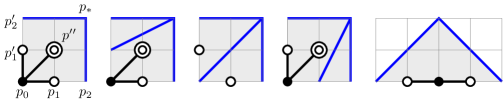
Figure 13. $D_{4}$ and its degenerations $A_{0}^{-}\kern-2.0pt\phantom{.}^{\prime}\kern-2.0pt\kern-1.0ptA_{3}$, $A_{1}A_{1}$, $A_{3}^{\prime}\raise 0.65pt\hbox{$\kern-2.0pt\phantom{.}^{-}$}\kern-4.0ptA_{0}$, $A_{3}$

Example 6.21.

An $ADE$ surface $(Y,C=C_{1}+C_{2})$ of shape $D_{4}$ is $Y={\mathbb{P}}^{1}\times{\mathbb{P}}^{1}$, with $C_{1}=s$, $C_{2}=f$ a section and a fiber. In an $ADE$ pair $(Y,C+\frac{1+\epsilon}{2}B)$, the divisor $B$ is in the linear system $|2s+2f|$. There are three obvious toric degenerations corresponding to removing the nodes $p^{\prime}_{1}$, $p_{0}$, $p_{1}$ in the Dynkin diagram, shown in the middle three pictures of Figure 13. In the degeneration corresponding to $p^{\prime}_{1}$ we get a 3-dimensional family of stable $ADE$ pairs with two components corresponding to $A_{0}^{-}\kern-2.0pt\phantom{.}^{\prime}\kern-2.0pt\kern-1.0ptA_{3}$. By symmetry, we get $A_{3}^{\prime}\raise 0.65pt\hbox{$\kern-2.0pt\phantom{.}^{-}$}\kern-4.0ptA_{0}$ surfaces for the node $p_{1}$.

The toric degeneration for the node $p_{0}$ is already somewhat unusual. Here ${\mathbb{P}}^{1}\times{\mathbb{P}}^{1}$ degenerates to ${\mathbb{P}}^{2}\cup{\mathbb{P}}^{2}$, and the stable $ADE$ pairs of shape $A_{1}A_{1}$ form only a 2-dimensional family, so some moduli are lost.

Additionally, there is an obvious nontoric degeneration of ${\mathbb{P}}^{1}\times{\mathbb{P}}^{1}$ to a quadratic cone ${\mathbb{P}}(1,1,2)$, with the limits of $C_{1},C_{2}$ passing through the vertex, and $B$ a double section. These are pairs of shape $A_{3}$ forming a 3-dimensional family.

Definition 6.22.

In the $\kern-2.0pt\phantom{.}^{\prime}\kern-2.0pt\kern-1.0ptA_{n}^{?}$, $D_{n}^{?}$, $\raise 0.65pt\hbox{$\kern-2.0pt\phantom{.}^{-}$}\kern-2.0ptE_{n}^{?}$ shapes, where $?$ denotes either no decoration or a $-$ depending upon the parity of $n$, we introduce the following elements of the homogeneous ring ${\mathbb{C}}[\Lambda^{*}][x,y][\xi]$:

$$u_{i}=e^{\varpi_{i}}x^{i}\cdot\xi^{2},\quad v_{2i}=e^{\varpi_{2i}/2}x^{i}\cdot\xi,\quad u^{\prime}_{i}=e^{\varpi^{\prime}_{i}}y^{i}\cdot\xi^{2},\quad v^{\prime}_{2i}=e^{\varpi^{\prime}_{2i}/2}y^{i}\cdot\xi.$$

We also have the $u$ variables for the left and right sides $p_{\ell}$, $p_{r}$ and, when these are even, their square roots, the $v$ variables. Additionally, we define a special non-monomial variable $v_{*}=(xy-c^{\prime\prime})\cdot\xi$ of degree 1.

As before, the coefficients $c=\chi(\varpi)$ are the characters of the fundamental weights, and we define the normalized characters by $\widehat{c}=e^{-\varpi}c$. With these notations, the naive families (5.6), (5.7), (5.8) become

(6.2) $$\kern-2.0pt\phantom{.}^{\prime}\kern-2.0pt\kern-1.0ptA_{n}^{?}: f=-\left(\frac{v_{*}}{2}\right)^{2}+u^{\prime}_{1}+\widehat{c}_{0}u_{0}+\widehat{c}_{1}u_{1}+\dotsb+\widehat{c}_{n-2}u_{n-2}+u_{n-1}$$

(6.3) $$D_{n}^{?}: f=-\left(\frac{v_{*}}{2}\right)^{2}+u^{\prime}_{2}+\widehat{c}^{\prime}_{1}u^{\prime}_{1}+\widehat{c}_{0}u_{0}+\widehat{c}_{1}u_{1}+\dotsb+\widehat{c}_{n-3}u_{n-3}+u_{n-2}$$

(6.4) $$\raise 0.65pt\hbox{$\kern-2.0pt\phantom{.}^{-}$}\kern-2.0ptE_{n}^{?}: f=-\left(\frac{v_{*}}{2}\right)^{2}+u^{\prime}_{3}+\widehat{c}^{\prime}_{2}u^{\prime}_{2}+\widehat{c}^{\prime}_{1}u^{\prime}_{1}+\widehat{c}_{0}u_{0}+\dotsb+\widehat{c}_{n-4}u_{n-4}+u_{n-3}$$

Definition 6.23.

Let $M$ be the lattice obtained by adjoining to $\Lambda^{*}$ the vectors $\varpi_{2i}/2$, $\varpi^{\prime}_{2i}/2$, $\alpha_{2i+1}/2$ (for all $i$), and $\alpha^{\prime\prime}/2$. Let $M^{+}=M\cap\sum_{\alpha}{\mathbb{R}}_{\geq 0}(-\alpha)$ and $R={\mathbb{C}}[M^{+}]$.

We define $a_{i}=e^{-\alpha_{i}}$, resp. $a^{\prime}_{i}=e^{-\alpha^{\prime}_{i}}$, for each node $p_{i}$ in the Dynkin diagram, and also $a^{\prime\prime}=e^{-\alpha^{\prime\prime}}$. For the odd nodes $p_{2i+1}$ we define $b_{2i+1}=e^{-\alpha_{2i+1}/2}$, resp. $b^{\prime}_{2i+1}=e^{-\alpha^{\prime}_{2i+1}/2}$, and also $b^{\prime\prime}=e^{-\alpha^{\prime\prime}/2}$.

Definition 6.24 (Compactified naive families for the $\kern-2.0pt\phantom{.}^{\prime}\kern-2.0pt\kern-1.0ptA,D,E$ shapes).

Let $S$ be the graded subring of $R[x,y][\xi]$ generated by $v_{2i}$, $u_{2i+1}$, $v^{\prime}_{2i}$, $u^{\prime}_{2i+1}$, and $v_{*}$. The compactified naive family is ${\mathcal{Y}}:=\operatorname{Proj}S\to\operatorname{Spec}R$ with a relative Cartier divisor ${\mathcal{B}}=(f)$, $f\in H^{0}({\mathcal{O}}(2))$. We note that since the subring $S^{(2)}$ is generated in degree 1, the sheaf ${\mathcal{O}}_{\operatorname{Proj}S}(2)$ is invertible and ample.

Lemma 6.25.

The following relations hold:

1. The same monomial relations as in Lemma 6.17 for the variables $u_{i},v_{i}$, with $i\geq 0$, and for the variables $u^{\prime}_{i}$, $v^{\prime}_{i}$, $v_{0}$.

2. A non-monomial “corner” relation $u_{1}u^{\prime}_{1}=a_{0}v_{0}^{3}(\widehat{c}^{\prime\prime}v_{0}+b^{\prime\prime}v_{*})$.

3. For each $u^{\prime}_{i},v^{\prime}_{i}$ variable and each $u_{i},v_{i}$ variable lying on the different sides of $v_{0}$, the same equations as in Lemma 6.17, but with $A=\frac{\widehat{c}^{\prime\prime}v_{0}+b^{\prime\prime}v_{*}}{v_{0}}\prod_{k=2i}^{2j}a_{k}$.

Proof.

We check the non-monomial relation. The LHS is $e^{\varpi_{1}+\varpi^{\prime}_{1}}xy\cdot\xi^{4}$. The RHS:

$$e^{-\alpha_{0}+\frac{3}{2}\varpi_{0}}\big{(}e^{-\varpi^{\prime\prime}+\frac{1}{2}\varpi_{0}}c^{\prime\prime}+e^{-\frac{1}{2}\alpha^{\prime\prime}}xy-e^{-\frac{1}{2}\alpha^{\prime\prime}}c^{\prime\prime}\big{)}\cdot\xi^{4}$$

The equality now follows from $-\varpi^{\prime\prime}+\frac{1}{2}\varpi^{\prime\prime}=-\frac{1}{2}\alpha^{\prime\prime}$ and $-\alpha_{0}+\frac{3}{2}\varpi_{0}-\frac{1}{2}\alpha^{\prime\prime}=\varpi_{1}+\varpi^{\prime}_{1}$, which hold because $\alpha^{\prime\prime}=2\varpi^{\prime\prime}-\varpi_{0}$ and $\alpha_{0}=2\varpi_{0}-\varpi_{1}-\varpi^{\prime}_{1}-\varpi^{\prime\prime}$. The proof of part (3) is formally the same as for the secondary monomial relations, with each term $\widehat{c}^{\prime\prime}v_{0}+b^{\prime\prime}v_{*}$ contributing an extra $xy$. ∎

Theorem 6.26.

The compactified families ${\mathcal{Y}}=\operatorname{Proj}S\to\operatorname{Spec}R$ of $\kern-2.0pt\phantom{.}^{\prime}\kern-2.0pt\kern-1.0ptA_{n}^{?}$, $D_{n}^{?}$, $\raise 0.65pt\hbox{$\kern-2.0pt\phantom{.}^{-}$}\kern-2.0ptE_{n}^{?}$ shapes are flat. The degenerate fibers are over the subsets given by setting some $a$’s to zero. Every fiber is a stable $ADE$ pair which is a union of $ADE$ pairs of shapes obtained as follows:

1. For the degenerations $a_{i}=0$ and $a^{\prime}_{i}=0$: by subdividing the corresponding polytope into integral subpolytopes by intervals from the vertex $p_{*}$ to the point $p_{i}$, resp. $p^{\prime}_{i}$.

2. For the degeneration $a^{\prime\prime}=0$: by “straightening the corner”, i.e. to the shape obtained by removing the node $p^{\prime\prime}$ from the Dynkin diagram.

The $W$-translates of these families glue into flat $W_{\Lambda}$-invariant families $({\mathcal{Y}},{\mathcal{C}}+\frac{1+\epsilon}{2}{\mathcal{B}})\to V^{\rm cox}_{M}$ of stable $ADE$ pairs over a torus embedding of $T_{M}=\operatorname{Hom}(M,{\mathbb{C}}^{*})$ for the Coxeter fan of $A_{n}$, resp. $D_{n}$, resp. $E_{n}$.

Proof.

The proof for the toric degenerations is the same as in Theorem 6.18. Gluing the family over $\operatorname{Spec}R$ to a $W$-invariant family over a projective toric variety for the Coxeter fan is also the same. We do not repeat these parts. Instead, we concentrate on the degenerations involving the corner relation (2) of Lemma 6.25.

When $a_{0}=0$ we get the toric relation $u_{1}u^{\prime}_{1}=0$ which as before gives a stable $ADE$ pair for the subdivision of our polytope into two polytopes obtained by cutting it from $p_{*}$ to $p_{0}$ into the shapes ${}^{?}A_{m^{\prime}}A^{?}_{m}$. The only observation here is that $m+m^{\prime}=n-2$, not $n-1$, so the moduli count drops by two, not one.

When $b^{\prime\prime}=0$, we also get $\widehat{c}^{\prime\prime}=1$ by Lemma 6.19, and the corner relation becomes $u_{1}u^{\prime}_{1}=a_{0}v_{0}^{4}$. Thus, the new set of relations is equivalent to those for the ${}^{?}\kern-3.0ptA_{n-1}^{?}$ shape. The equations (6.2), (6.3), (6.4) reduce to the equation (6.1). ∎

6D. Compactifications of the naive families for all primed shapes

Theorems 6.18, 6.26 describe all stable $ADE$ pairs that appear as degenerations of $ADE$ pairs of pure shapes. In particular, irreducible components of degenerate pairs $(Y,C+\frac{1+\epsilon}{2}B)$ are normal, and they are $ADE$ pairs for smaller shapes. For some degenerations of pairs of primed shapes the folded shapes of Definition 6.9 appear.

Definition 6.27.

The Priming Rules are $A^{\prime}_{1}\to A_{0}^{-}$, $\kern-2.0pt\phantom{.}^{\prime}\kern-2.0pt\kern-1.0ptA_{1}\to\raise 0.65pt\hbox{$\kern-2.0pt\phantom{.}^{-}$}\kern-4.0ptA_{0}$; $\raise 0.65pt\hbox{$\kern-2.0pt\phantom{.}^{-}$}\kern-4.0ptA^{\prime}_{0}\to 0$, $\kern-2.0pt\phantom{.}^{\prime}\kern-2.0pt\kern-1.0ptA^{-}_{0}\to 0$; and $A_{0}^{+}\to f$, $\raise 0.65pt\hbox{$\kern-2.0pt\phantom{.}^{+}$}\kern-4.0ptA_{0}\to f$ are folds applied to the neighboring surface.

Theorem 6.28.

For each primed shape, there exists a flat family of stable $ADE$ pairs $({\mathcal{Y}},{\mathcal{C}}+\frac{1+\epsilon}{2}{\mathcal{B}})\to V^{\rm cox}_{M}$ over the a torus embedding of $\operatorname{Hom}(M,{\mathbb{C}}^{*})$ for the Coxeter fan of $A_{n}$, resp. $D_{n}$, resp. $E_{n}$, where $M$ is the lattice defined in (6.13) for the $A$ shapes and (6.23) for $D,E$ shapes. The fibers over the toric strata of $V^{\rm cox}_{M}$ are computed by starting with the fibers of the family for the pure shape and then applying the Priming Rules one prime at a time.

Example 6.29.

We list the degenerate fibers in the compactified families for the pure shape $A_{2}^{-}$ (see Fig. 12) and the corresponding fibers in the families for the primed shapes $\kern-2.0pt\phantom{.}^{\prime}\kern-2.0pt\kern-1.0ptA_{2}^{-}$, $\kern-2.0pt\phantom{.}^{\prime\prime}\kern-2.0pt\kern-1.0ptA_{2}^{-}$, $A_{2}^{+}$.

$$\begin{array}[]{l|lll}\text{shape}&\lx@intercol\hfil\text{shapes of degenerations}\hfil\lx@intercol\\ \hline\cr A_{2}^{-}&A_{0}^{-}\raise 0.65pt\hbox{$\kern-2.0pt\phantom{.}^{-}$}\kern-4.0ptA_{1}^{-}&A_{1}A_{0}^{-}&A_{0}^{-}\raise 0.65pt\hbox{$\kern-2.0pt\phantom{.}^{-}$}\kern-4.0ptA_{0}A_{0}^{-}\\ \kern-2.0pt\phantom{.}^{\prime}\kern-2.0pt\kern-1.0ptA_{2}^{-}&\kern-2.0pt\phantom{.}^{\prime}\kern-2.0pt\kern-1.0ptA_{0}^{-}\raise 0.65pt\hbox{$\kern-2.0pt\phantom{.}^{-}$}\kern-4.0ptA_{1}^{-}\to\raise 0.65pt\hbox{$\kern-2.0pt\phantom{.}^{-}$}\kern-4.0ptA_{1}^{-}&\kern-2.0pt\phantom{.}^{\prime}\kern-2.0pt\kern-1.0ptA_{1}A_{0}^{-}\to\raise 0.65pt\hbox{$\kern-2.0pt\phantom{.}^{-}$}\kern-4.0ptA_{0}A_{0}^{-}&\kern-2.0pt\phantom{.}^{\prime}\kern-2.0pt\kern-1.0ptA_{0}^{-}\raise 0.65pt\hbox{$\kern-2.0pt\phantom{.}^{-}$}\kern-4.0ptA_{0}A_{0}^{-}\to\raise 0.65pt\hbox{$\kern-2.0pt\phantom{.}^{-}$}\kern-4.0ptA_{0}A_{0}^{-}\\ \kern-2.0pt\phantom{.}^{\prime\prime}\kern-2.0pt\kern-1.0ptA_{2}^{-}&\raise 0.65pt\hbox{$\kern-2.0pt\phantom{.}^{+}$}\kern-4.0ptA_{1}^{-}&\raise 0.65pt\hbox{$\kern-2.0pt\phantom{.}^{+}$}\kern-4.0ptA_{0}A_{0}^{-}\to\raise 1.17pt\hbox{$\kern-2.0pt\phantom{.}^{f}$}\kern-4.0ptA_{0}^{-}&\raise 0.65pt\hbox{$\kern-2.0pt\phantom{.}^{+}$}\kern-4.0ptA_{0}A_{0}^{-}\to\raise 1.17pt\hbox{$\kern-2.0pt\phantom{.}^{f}$}\kern-4.0ptA_{0}^{-}\\ A_{2}^{+}&A_{0}^{-}\raise 0.65pt\hbox{$\kern-2.0pt\phantom{.}^{-}$}\kern-4.0ptA_{1}^{+}&A_{1}A_{0}^{+}\to A_{1}^{f}&A_{0}^{-}\raise 0.65pt\hbox{$\kern-2.0pt\phantom{.}^{-}$}\kern-4.0ptA_{0}A_{0}^{+}\to A_{0}^{-}\raise 0.65pt\hbox{$\kern-2.0pt\phantom{.}^{-}$}\kern-4.0ptA_{0}^{f}\end{array}$$

Before proving the theorem, we explain the meaning of the Priming Rules.

Lemma 6.30.

One has the following:

1. Priming a surface of shape $A_{1}$ gives a surface of shape $A^{-}_{0}$.

2. Priming a surface $Y$ of shape $\raise 0.65pt\hbox{$\kern-2.0pt\phantom{.}^{-}$}\kern-4.0ptA_{0}$ on the long side $C_{2}$ gives a surface $Y^{\prime}$ and a nef line bundle $L^{\prime}$ such that $(L^{\prime})^{2}=0$ and $|L^{\prime}|$ contracts $Y^{\prime}$ to ${\mathbb{P}}^{1}$, with the other side $C_{1}$ mapping isomorphically to ${\mathbb{P}}^{1}$.

3. Priming a surface $Y$ of shape $\raise 0.65pt\hbox{$\kern-2.0pt\phantom{.}^{-}$}\kern-4.0ptA_{0}$ on the short side $C_{1}$ gives a surface $Y^{\prime}$ and a nef line bundle $L^{\prime}$ such that $(L^{\prime})^{2}=0$ and $|L^{\prime}|$ contracts $Y^{\prime}$ to ${\mathbb{P}}^{1}$, with the other side $C_{2}$ folding 2:1 to ${\mathbb{P}}^{1}$.

Proof.

We proved in (1) in Theorem 3.18 already, see also Remark 3.20. Parts (2,3) are easy computations. ∎

Proof of Thm. 6.28.

Let $f\colon({\mathcal{Y}},{\mathcal{C}}+\frac{1+\epsilon}{2}{\mathcal{B}})\to V^{\rm cox}_{M}$ be a family for a pure shape. It comes with canonical sections: one for a short side of the shape, and two disjoint sections for a long side. Now make a weighted blow up one of the sections to obtain a family $f^{\prime}\colon({\mathcal{Y}}^{\prime},{\mathcal{C}}^{\prime}+\frac{1+\epsilon}{2}{\mathcal{B}}^{\prime})\to V^{\rm cox}_{M}$. Then the sheaf ${\mathcal{L}}^{\prime}={\mathcal{O}}_{{\mathcal{Y}}^{\prime}}(-2(K_{{\mathcal{Y}}^{\prime}/Z}+C^{\prime})$ is invertible and relatively nef. As in proof of Theorem 3.18, this sheaf is relatively semiample and gives a contraction ${\mathcal{Y}}^{\prime}\to\overline{{\mathcal{Y}}^{\prime}}$ to a family $\bar{f}^{\prime}\colon(\overline{{\mathcal{Y}}^{\prime}},\overline{{\mathcal{C}}^{\prime}}+\frac{1+\epsilon}{2}\overline{{\mathcal{B}}^{\prime}})\to V^{\rm cox}_{M}$ over the same base. For a reducible fiber $Y^{\prime}=\cup Y^{\prime}_{k}$ of the family $f^{\prime}$, the sheaf ${\mathcal{L}}^{\prime}$ is ample on all components $Y^{\prime}_{k}$ except possibly on the blown up surface on the end. For this surface the resulting surface ${\overline{Y}}^{\prime}_{k}$ is given by Lemma 6.30. The other sections of ${\mathcal{Y}}\to V^{\rm cox}_{M}$ map to disjoint sections of $\overline{{\mathcal{Y}}^{\prime}}\to V^{\rm cox}_{M}$. We then repeat the process for the second prime, etc. ∎

Remark 6.31.

Theorem 6.28 extends to the degenerations of surfaces of shapes with folds, e.g. $A_{2n-1}^{f}$ as follows: the degenerations are the same as for the shape with a long side, but that long side is folded.

6E. A generalized Coxeter fan

As Examples 6.21 and 6.29 show, the families $({\mathcal{Y}},{\mathcal{C}}+\frac{1+\epsilon}{2}{\mathcal{B}})\to V^{\rm cox}_{M}$ over the projective toric variety for the Coxeter fan have repeating fibers over certain boundary strata. Here we define a coarser generalized Coxeter fan and a birational contraction $\rho\colon V^{\rm cox}_{M}\to V^{\rm semi}_{M}$ such that the families are constant on the fibers of $\rho$ and such that the correspondence between the isomorphism classes of the pairs $(Y,C+\frac{1+\epsilon}{2}B)$ and the points of $V^{\rm semi}_{M}$ is finite to one.

The Coxeter fan $\tau^{\rm cox}$ on the vector space $N_{\mathbb{R}}=\Lambda_{\mathbb{R}}=\Lambda^{*}_{\mathbb{R}}$ is obtained by cutting it with the mirror hyperplanes $\alpha^{\perp}$ for the roots $\alpha\in\Lambda$. Another definition is: it is the normal fan to the permutahedron, $\operatorname{Conv}(W_{\Lambda}.p)$, the convex hull of the $W_{\Lambda}$-orbit of a generic point $p$ in the interior of the positive chamber $C^{+}=\{\alpha\geq 0\}$, where $\Delta=\{\alpha\}$ are the simple roots. In particular, the maximal cones of the Coxeter fan are in a bijection with the vertices of $\operatorname{Conv}(W_{\Lambda}.p)$ and with the elements of the Weyl group $W=W_{\Lambda}$.

Definition 6.32.

For a proper subset $\Delta^{0}\subset\Delta$ of the simple roots, let $p\in C^{+}$ be a point such that $\alpha\cdot p=0$ for $\alpha\in\Delta^{0}$ and $\alpha\cdot p>0$ for $\alpha\in\Delta\setminus\Delta^{0}$. A generalized permutahedron is the convex hull $\operatorname{Conv}(W_{\Lambda}.p)$ and a generalized Coxeter fan $\tau^{\rm semi}$ is defined to be its normal fan.

Definition 6.33.

We will call $\Delta^{0}$ the irrelevant subset. For $S\subset\Delta$ we define its relevant content $S^{\rm rel}$ to be the union of the connected components not lying in $\Delta^{0}$. We will call a connected component $S^{\prime}$ of $S\subset\Delta$ irrelevant if $S^{\prime}\subset\Delta^{0}$.

The proof of the following lemma is straightforward.

Lemma 6.34.

1. The $W$-orbits of cones of $\tau^{\rm cox}$ are in bijection with the subsets $S\subset\Delta$ via: $S\mapsto\operatorname{Conv}(W_{S}.p)$, where $W_{S}\subset W_{\Lambda}$ is the Weyl subgroup generated by the simple roots $\alpha\in S$.

2. The $W$-orbits of cones of $\tau^{\rm cox}$ are in bijection with the subsets without irrelevant connected components.

3. The fan $\tau^{\rm semi}$ is a coarsening of the fan $\tau^{\rm cox}$ and the morphism $\rho\colon V^{\rm cox}\to V^{\rm semi}$ of the corresponding projective toric varieties is proper and birational.

4. The image of a torus orbit $O_{S}\subset V^{\rm cox}$ is $O_{S^{\rm rel}}\subset V^{\rm semi}$. One has $\dim O_{S}=|S|$ and $\dim O_{S^{\rm rel}}=|S^{\rm rel}|$. If $S$ has no irrelevant components the morphism $O_{S}~{}\xrightarrow{\sim}~{}O_{S^{\rm rel}}$ is an isomorphism.

Definition 6.35.

For a decorated Dynkin diagram of a (possibly primed) shape, we define the irrelevant subset $\Delta^{0}\subset\Delta$ to be the set of circled white (i.e. unfilled) nodes.

Example 6.36.

In the pure $D,\raise 0.65pt\hbox{$\kern-2.0pt\phantom{.}^{-}$}\kern-2.0ptE$ shapes, and also in the toric $\kern-2.0pt\phantom{.}^{\prime}\kern-2.0pt\kern-1.0ptA$ shape, the interior circled white node is irrelevant, see Figs. 2, 3, 7. In the toric shapes $D^{\prime}$ and $\kern-2.0pt\phantom{.}^{\prime}\kern-2.0pt\kern-1.0ptA^{\prime}$ the irrelevant subset consists of two nodes, see Fig. 8. In the primed shapes there may be more irrelevant nodes, cf. Fig 6.

Theorem 6.37.

The pairs in the family $({\mathcal{Y}},{\mathcal{C}}+\frac{1+\epsilon}{2}{\mathcal{B}})\to V^{\rm cox}_{M}$ are isomorphic on each fiber of the contraction $\rho\colon V^{\rm cox}_{M}\to V^{\rm semi}_{M}$. The correspondence between the points of $V^{\rm semi}_{M}$ and the isomorphism classes of the pairs $(Y,C+\frac{1+\epsilon}{2}B)$ is finite to one.

Proof.

Consider a codimension 1 orbit of $V^{\rm cox}_{M}$ corresponding to setting $a=e^{-\alpha}$ to zero for a single node of the Dynkin diagram $p$. By Theorems 6.26 and 6.28 the dimension of the family over the boundary stratum drops by 2 instead of the expected 1 exactly when one of the following happens:

1. In the $\kern-2.0pt\phantom{.}^{\prime}\kern-2.0pt\kern-1.0ptA$, $D$, $E$ shapes, we remove the corner node $p_{0}$, leaving the circled white node $p^{\prime\prime}$ isolated.

2. A single left-most or right-most white node which in our shape is primed or doubly primed (so white and circled) becomes an isolated $A_{1}^{\prime}$ or $\kern-2.0pt\phantom{.}^{\prime}\kern-2.0pt\kern-1.0ptA_{1}$ after a node next to it is removed.

In both cases this happens precisely when the subdiagram $S=\Delta-p$ corresponding to the codimension 1 orbit of $V^{\rm cox}_{M}$ has an irrelevant component, a single node.

We now observe that for any shape the irrelevant subset consists of several disjoint isolated nodes. There is a drop in the moduli count by one for each of them. On the other hand, for the orbits $O_{S}$ for $S$ without irrelevant components, the restriction of the family to $O_{S}$ is the naive family for the Dynkin diagram $S$. The set of the isomorphism classes in the latter family is $O_{S}$ modulo a finite Weyl group $W_{S}\rtimes W_{0}$ and a finite multiplicative group $\mu_{S}$. This proves the statement. ∎

6F. Description of the compactified moduli space of $ADE$ pairs

We now prove Theorem C. In fact we will prove the following slightly stronger result, which contains more information about the toric primed shapes.

Theorem 6.38.

For each $ADE$ shape the moduli space $M^{\rm slc}_{ADE}$ is proper and the stable limit of $ADE$ pairs are stable $ADE$ pairs.

1. For the pure $ADE$ shapes, the normalization $(M^{\rm slc}_{ADE})^{\nu}$ is $V^{\rm semi}_{\Lambda}/W_{\Lambda}$, a $W_{\Lambda}$-quotient of the projective toric variety for the generalized Coxeter fan.

2. For the toric primed shapes $\kern-2.0pt\phantom{.}^{\prime}\kern-2.0pt\kern-1.0ptA_{2n-1}$, $\kern-2.0pt\phantom{.}^{\prime}\kern-2.0pt\kern-1.0ptA_{2n-2}^{-}$, $\kern-2.0pt\phantom{.}^{\prime}\kern-2.0pt\kern-1.0ptA_{2n-1}^{\prime}$, $D_{2n}^{\prime}$ with $n\geq 3$, the normalization $(M^{\rm slc}_{ADE})^{\nu}$ is $V^{\rm semi}_{\Lambda^{\prime}}/W_{\Lambda}$ with the lattice $\Lambda^{\prime}$ described in (5.11).

3. For an arbitrary primed shape, the normalization $(M^{\rm slc}_{ADE})^{\nu}$ is $V^{\rm semi}_{\Lambda^{\prime}}/W_{\Lambda}\rtimes W_{0}$, for a lattice extension $\Lambda^{\prime}\supset\Lambda$. The lattice $\Lambda^{\prime}$ and the Weyl group $W_{0}$ are described in (5.12).

Proof.

(1) By Theorems 6.18, 6.26, 6.28, every one-parameter family of $ADE$ pairs has a limit which is a stable $ADE$ pair, since it has a limit (after a finite base change) in the family over $V^{\rm cox}_{M}$. By Theorem 6.37 the classifying morphism $\phi\colon V^{\rm semi}_{M}/W\to M^{\rm slc}_{ADE}$ is finite-to-one. By Theorem 5.9 on a dense open set it equals $\operatorname{Hom}(M,{\mathbb{C}}^{*})/W\to\operatorname{Hom}(\Lambda,{\mathbb{C}}^{*})/W$, and it factors through the homomorphism $\operatorname{Hom}(M,{\mathbb{C}}^{*})\to\operatorname{Hom}(\Lambda,{\mathbb{C}}^{*})$, the quotient by the finite multiplicative group $\mu:=\operatorname{Hom}(M/\Lambda,{\mathbb{C}}^{*})$. Thus, $\phi$ factors through $V^{\rm semi}_{\Lambda}=V^{\rm semi}_{M}/\mu$, and the morphism $V^{\rm semi}_{M}\to M^{\rm slc}_{ADE}$ is finite to one and an isomorphism over an open dense subset. Since $V^{\rm semi}_{M}$ is normal, it is the normalization of $M^{\rm slc}_{ADE}$.

Parts (2) and (3) are proved the same way. ∎

Remark 6.39.

Theorem 6.38 extends to surfaces of shapes with folds, e.g. $A_{2n-1}^{f}$, cf. Remark 6.31.

7. Canonical families and their compactifications

In the previous Section we compactified the stack of $ADE$ pairs – which for the pure shapes is $[{\mathbb{A}}^{n}:\mu_{\Lambda}]$ – and extended the naive family over it to a family of stable pairs. However, $[{\mathbb{A}}^{n}:\mu_{\Lambda}]$ has many automorphisms, and consequently in the equation $f$ of the divisor $B$ we have a lot of freedom for the coefficients $c_{i}=c_{i}(\chi_{1},\dotsc,\chi_{n})$ as polynomials in the fundamental characters. Many of these choices extend to the compactification.

Example 7.1.

For the $A_{1}$ shape the moduli stack is $[{\mathbb{A}}^{1}:\mu_{2}]$, and we write ${\mathbb{A}}^{1}$ as the quotient of the torus ${\mathbb{C}}^{*}_{t}$ by the Weyl group $W_{\Lambda}={\mathbb{Z}}_{2}$, $t\to t^{-1}$. The compactification is $[{\mathbb{P}}^{1}:\mu_{2}]$. The equation of $B$ is $f=1+c_{1}x+x^{2}$, where in the naive family we have $c_{1}=\chi_{1}=t+t^{-1}$. We can apply to ${\mathbb{A}}^{1}$ an automorphism $c_{1}\mapsto ac_{1}+b$, with $a,b\in{\mathbb{C}}$ and $a\neq 0$, then pull the family back to ${\mathbb{C}}^{*}_{t}$. This automorphism extends to the compactification ${\mathbb{P}}^{1}$ of ${\mathbb{A}}^{1}$, but the coordinate change is not compatible with the $\mu_{\Lambda}$-action (i.e. with the $(\Lambda^{*}/\Lambda)$-grading) unless $b=0$, since $(-1)\in\mu_{2}$ acts by $ac_{1}+b\mapsto-ac_{1}+b$, so it is not an automorphism of $[{\mathbb{A}}^{1}:\mu_{2}]$. In this case the naive family is effectively unique.

However, for the root systems $D_{n}$ ($n\geq 5$) and $E_{n}$ ($n=6,7,8$) there exist dominant weights $\lambda<\varpi_{i}$ lying below the fundamental weights and with $\lambda\equiv\varpi_{i}$ in $\Lambda^{*}/\Lambda$, and we can modify the coefficients $c_{i}=\chi_{i}$ by adding linear combinations of their characters $\chi(\lambda)$. For example, for $E_{8}$ there are 23 dominant weights $\lambda$ below $\varpi_{0}$, and $\Lambda^{*}/\Lambda=0$. Counting all fundamental weights $\varpi$ and their lower terms, there is a ${\mathbb{C}}^{51}$ worth of choices for $c=\chi(\varpi)+\sum_{\lambda<\varpi}c_{\lambda}\chi(\lambda)$, all extending to automorphisms of our moduli compactification.

In this Section we show that the naive family can be deformed in an essentially unique way so that the new family, which we call the canonical family, has the following wonderful property: the discriminant locus in $T_{\Lambda}$, over which the divisor $B$ in our $ADE$ pairs become singular, is a union of root hypertori $\{e^{\alpha}=1\}$, with $\alpha$ going over the roots of the lattice $\Lambda$.

We then show that the canonical family extends to the compactification and that on the boundary strata it restricts to the canonical families for smaller Dynkin diagrams.

7A. Two notions of the discriminant

Let $f(x,y)$ be one of the polynomials in the equations (5.4)–(5.8), which we related to the root lattices $\Lambda=A_{n}$, $D_{n}$, $E_{n}$. There are two different notions of the discriminant in this situation:

1. The discriminant $\operatorname{Discr}(f)$ of a polynomial $f(x,y)$. This is a polynomial in the coefficients $c_{i}$ of $f$ for which the zero set of $f$ on $Y\setminus C$ is singular. If $c_{i}=c_{i}(\chi_{j})$ are polynomials in the fundamental characters of the lattice $\Lambda$, then $\operatorname{Discr}(f)$ becomes a polynomial in $\chi_{j}$.

2. The discriminant $\operatorname{Discr}(\Lambda)$ of the lattice, the square of the expression

   $$\prod_{\alpha\in\Phi^{+}}(e^{\alpha/2}-e^{-\alpha/2})=\sum_{w\in W_{\Lambda}}\varepsilon(w)e^{w.\rho},\quad\text{where }\rho=\sum_{\varpi\in\Pi}\varpi=\frac{1}{2}\sum_{\alpha\in\Phi^{+}}\alpha.$$

   appearing in the Weyl character formula. $\operatorname{Discr}(\Lambda)$ is $W_{\Lambda}$-invariant, so it is also a polynomial in the fundamental characters. The zero set of $\operatorname{Discr}(\Lambda)$ is obviously the union of the root hypertori $e^{\alpha}=1$.

The following theorem forms the first part of Theorem D. We prove it separately for the $A,D,E$ shapes in Theorems 7.3, 7.5, 7.7, respectively.

Theorem 7.2.

For each $ADE$ pair of pure shape, there exists a unique deformation of the form $c=\chi(\varpi)+\text{(lower terms)}$ of the naive equation such that $\operatorname{Discr}(f)=\operatorname{Discr}(\Lambda)$.

7B. Canonical families

Theorem 7.3 ($A$ shapes).

For the pure shapes $A_{n}^{?}$, resp. $\raise 0.65pt\hbox{$\kern-2.0pt\phantom{.}^{-}$}\kern-4.0ptA_{n}^{?}$, in Theorem 7.2 one has $c_{i}=\chi_{i}$, resp. $c_{i}=\chi_{i-1}$.

Proof.

For $A_{n}^{?}$ the curve $-\frac{1}{4}y^{2}+c(x)$ is singular iff $c(x)$ has a double root. If

$$c(x)=\prod_{i=1}^{n+1}(x+t_{i})=1+\chi_{1}x+\dotsc+\chi_{n}x^{n}+x^{n+1}$$

then this happens iff $e^{e_{i}-e_{j}}=t_{i}/t_{j}=1$. Here, $e_{i}-e_{j}$ are precisely the roots of $A_{n}$. Thus, the statement holds for $c_{i}=\chi_{i}$. For $A_{n}$ there are no lower weights below the fundamental weights, so the solution is unique. The open sets $Y\setminus C$ for the shapes $A_{n}^{?}$ and $\raise 0.65pt\hbox{$\kern-2.0pt\phantom{.}^{-}$}\kern-4.0ptA_{n}^{?}$ are the same, so this argument applies to the $\raise 0.65pt\hbox{$\kern-2.0pt\phantom{.}^{-}$}\kern-4.0ptA_{n}^{?}$ shapes as well. ∎

Recall from section 5E that for the $D$ and $E$ shapes there are two equivalent forms of the equation: $F(x,y,z)$ and $f(x,y)$, and the latter is obtained from the former by completing the square in $z$. For $D_{n}$ one has the following root lattice, weight lattice, Weyl group, fundamental roots $\alpha_{i}$, and fundamental weights $\varpi_{i}$:

$$\Lambda=\left\{(a_{i})\in{\mathbb{Z}}^{n}=\oplus{\mathbb{Z}}e_{i}\mid\sum a_{i}\text{ is even}\right\},\quad\Lambda^{*}={\mathbb{Z}}^{n}+\frac{1}{2}\sum e_{i}.$$

$$W_{\Lambda}={\mathbb{Z}}_{2}^{n-1}\rtimes S_{n},$$

$$\alpha_{n-2-i}=e_{i}-e_{i+1}\text{ for }i\leq n-2,\ \alpha_{1}^{\prime}=e_{n-1}-e_{n},\ \alpha^{\prime\prime}=e_{n-1}+e_{n}.$$

$$\varpi_{n-2-i}=\sum_{k=1}^{i}e_{k}\text{ for }i\leq n-2,\ \varpi^{\prime}_{1}=\frac{1}{2}\left(-e_{n}+\sum_{i=1}^{n-1}e_{i}\right),\ \varpi^{\prime\prime}=\frac{1}{2}\left(\sum_{i=1}^{n}e_{i}\right).$$

Denoting by $\sigma_{i}$ the $i$-th symmetric polynomial, the fundamental characters are

$$\chi_{i}=\sigma_{n-2-i}(t_{k}^{\pm})\text{ for }i\leq n-2,\ \chi^{\prime}_{1}=\frac{\sum_{s\geq 0}\sigma_{2s+1}(t_{k})}{\sqrt{\prod t_{k}}},\ \chi^{\prime\prime}=\frac{\sum_{s\geq 0}\sigma_{2s}(t_{k})}{\sqrt{\prod t_{k}}},$$

where $t_{k}^{\pm}$ are $t_{1},t_{1}^{-1},\dotsc,t_{n},t_{n}^{-1}$.

Definition 7.4.

Let $f_{k}(x)$ be the polynomials defined recursively by $f_{0}=1$, $f_{1}=x$, and $f_{k+2}=xf_{k+1}-f_{k}$. These are the Fibonacci polynomials, except for the signs and a shift in degrees by 1. One has $f_{2}=x^{2}-1$, $f_{3}=x^{3}-2x$, etc.

Theorem 7.5 ($D$ shapes).

For the $D_{n}^{?}$ shapes, in Theorem 7.2 one has $c^{\prime}_{1}=\chi^{\prime}_{1}$, $c^{\prime\prime}=\chi^{\prime\prime}$, and the expression for $c(x)$ can be obtained from the generating function

$$c(x,\chi)=\sum_{i,j\geq 0}c_{ij}x^{i}\chi^{j}=\sum_{i\geq 0}c_{i}(\chi)x^{i}=\sum_{j\geq 0}p_{j}(x)\chi^{j}$$

by substituting $\chi_{j}$ for $\chi^{j}$ and setting $\chi_{n-2}=1$ and $\chi_{j}=0$ for $j>n-2$. One has

1. $\displaystyle c(x,\chi)=\frac{1}{(1-\chi^{2})(1-x\chi+\chi^{2})}$ and $\displaystyle c_{i}(\chi)=\frac{\chi^{i}}{(1-\chi^{4})(1+\chi^{2})^{i}}$.

2. $p_{2k}(x)=f_{k}^{2}$ and $p_{2k+1}=f_{k}f_{k+1}$.

3. $c_{ij}=0$ if $j-i$ is odd or $i>j$. Otherwise,

   $$c_{i,i+2k}=\sum_{p\geq 0}^{k}(-1)^{p}{i+p\choose i}=(-1)^{k}\sum_{q\geq 0}{i+k-1-2q\choose i-1}.$$

The central fiber has a $D_{n}$ singularity at the point $(x,y,z)=(-2,-2^{n-3},-2^{n-3})$.

Example 7.6.

For $D_{7}$ we obtain for the following expressions for $c(x)$:

$$\chi_{0}+\chi_{1}x+\chi_{2}x^{2}+\chi_{3}x(x^{2}-1)+\chi_{4}(x^{2}-1)^{2}+(x^{2}-1)(x^{3}-2x)=$$

$$(\chi_{0}+\chi_{4})+(\chi_{1}-\chi_{3}+2)x+(\chi_{2}-2\chi_{4})x^{2}+(\chi_{3}-3)x^{3}+\chi_{4}x^{4}+x^{5}$$

and for any lower $D_{n}$ the formulas can be obtained from these by truncation.

Proof of Thm. 7.5.

We start with the polynomial $f(x,y)$ in equation (5.7). As a quadratic polynomial in $y$, it represents a curve which is a double cover of ${\mathbb{A}}^{1}$. This curve is singular when the following polynomial in $x$

$$\operatorname{Discr}_{y}(f)=(x^{2}-4)c(x)+c^{\prime}_{1}c^{\prime\prime}x+c^{\prime}_{1}{}^{2}+c^{\prime\prime}{}^{2}$$

has a double root. On the other hand, the polynomial $p(x)=\prod_{i=1}^{n}(x+t_{i}+t_{i}^{-1})$ has a double root iff some $t_{i}+t_{i}^{-1}=t_{j}+t_{j}^{-1}$, i.e. $t_{i}t_{j}^{-1}=1$ or $t_{i}t_{j}=1$. These are exactly the root hypertori for the root lattice $D_{n}$.

Thus, $\operatorname{Discr}(f)=\operatorname{Discr}(\Lambda)$ iff $\operatorname{Discr}_{y}(f)=p(x)$. The coefficients of $p(x)$ are $\sigma_{i}(t_{k}+t_{k}^{-1})$, and they are invariant under the $W(D_{n})$-action, so they are polynomials in the fundamental characters $\chi_{i}$ listed above. The rest of the proof is a combinatorial manipulation to get the exact formula. From this procedure we see that the solution is unique. ∎

Theorem 7.7 ($E$ shapes).

For the $\raise 0.65pt\hbox{$\kern-2.0pt\phantom{.}^{-}$}\kern-2.0ptE_{n}^{?}$ shapes, in Theorem 7.2 one has

1. $$c^{\prime\prime}=\chi^{\prime\prime}-6\qquad c^{\prime}_{2}=\chi^{\prime}_{2}\qquad c^{\prime}_{1}=\chi^{\prime}_{1}-\chi_{2}$$

   $$c_{0}=\chi_{0}-3\chi^{\prime\prime}+9\qquad c_{1}=\chi_{1}-\chi^{\prime}_{2}\qquad c_{2}=\chi_{2}\qquad$$

2. $$c^{\prime\prime} =\chi^{\prime\prime}-6\chi_{3}\qquad c^{\prime}_{2}=\chi^{\prime}_{2}-25\qquad c^{\prime}_{1}=\chi^{\prime}_{1}-\chi_{2}-16\chi^{\prime}_{2}+206$$

   $$c_{0} =\chi_{0}-3\chi(\varpi^{\prime\prime}+\varpi_{3})+\chi(2\varpi^{\prime}_{2})-12\chi^{\prime}_{1}+9\chi(2\varpi_{3})+16\chi_{2}+69\chi^{\prime}_{2}-548$$

   $$c_{1} =\chi_{1}-\chi(\varpi^{\prime}_{2}+\varpi_{3})-6\chi^{\prime\prime}+28\chi_{3}\qquad c_{2}=\chi_{2}-2\chi^{\prime}_{2}+23\qquad c_{3}=\chi_{3}$$

3. $$c^{\prime\prime} =\chi^{\prime\prime}-6\chi_{3}-35\chi^{\prime}_{2}+920\chi_{4}-57505\qquad c^{\prime}_{2}=\chi^{\prime}_{2}-25\chi_{4}+2325$$

   $$c^{\prime}_{1} =\chi^{\prime}_{1}-\chi_{2}-16\chi(\varpi^{\prime}_{2}+\varpi_{4})-44\chi^{\prime\prime}+206\chi(2\varpi_{4})+$$

   $$+360\chi_{3}+2196\chi^{\prime}_{2}-51246\chi_{4}+2401900$$

   $$c_{0} =\chi_{0}-3\chi(\varpi^{\prime\prime}+\varpi_{3})+\chi(2\varpi^{\prime}_{2}+\varpi_{4})-12\chi(\varpi^{\prime}_{1}+\varpi_{4})-28\chi(\varpi^{\prime}_{2}+\varpi^{\prime\prime})+$$

   $$+9\chi(2\varpi_{3})+16\chi(\varpi_{2}+\varpi_{4})-68\chi_{1}+69\chi(\varpi^{\prime}_{2}+2\varpi_{4})+212\chi(\varpi^{\prime}_{2}+\varpi_{3})+$$

   $$+1024\chi(\varpi^{\prime\prime}+\varpi_{4})+236\chi(2\varpi^{\prime}_{2})+2453\chi^{\prime}_{1}-548\chi(3\varpi_{4})-$$

   $$-5228\chi(\varpi_{3}+\varpi_{4})-1507\chi_{2}-42656\chi(\varpi^{\prime}_{2}+\varpi_{4})-107636\chi^{\prime\prime}+$$

   $$+488553\chi(2\varpi_{4})+640064\chi_{3}+2988404\chi^{\prime}_{2}-52027360\chi_{4}+1484779780$$

   $$c_{1} =\chi_{1}-\chi(\varpi^{\prime}_{2}+\varpi_{3})-6\chi(\varpi^{\prime\prime}+\varpi_{4})+2\chi(2\varpi^{\prime}_{2})-17\chi^{\prime}_{1}+$$

   $$+28\chi(\varpi_{3}+\varpi_{4})-79\chi_{2}+383\chi(\varpi^{\prime}_{2}+\varpi_{4})+1429\chi^{\prime\prime}-$$

   $$-4414\chi(2\varpi_{4})+84\chi_{3}-49768\chi^{\prime}_{2}+271934\chi_{4}+4528192$$

   $$c_{2} =\chi_{2}-2\chi(\varpi^{\prime}_{2}+\varpi_{4})-9\chi^{\prime\prime}+23\chi(2\varpi_{4})-114\chi_{3}+601\chi^{\prime}_{2}+7673\chi_{4}-955955$$

   $$c_{3} =\chi_{3}-3\chi^{\prime}_{2}-170\chi_{4}+23405\qquad c_{4}=\chi_{4}-248$$

The central fiber with an $E_{6}$, resp. $E_{7}$, resp. $E_{8}$ singularity is

1. $xyz=z^{2}+72z+y^{3}+27y^{2}+324y+2700+324x+27x^{2}+x^{3}$ at $(x,y,z)=(-6,-6,-18)$.

2. $xyz=z^{2}+576z+y^{3}+108y^{2}+5184y+193536+17280x+1296x^{2}+56x^{3}+x^{4}$ at $(x,y,z)=(-12,-24,-144)$.

3. $xyz=z^{2}+y^{3}+x^{5}$ at $(0,0,0)$.

The formulas for the polynomials $F(x,y,z)$ were found by Etingof, Oblomkov, Rains in [EOR07] in a completely different context, as relations for the centers of certain non-commutative algebras associated to affine star-shaped Dynkin diagrams ${\widetilde{D}}_{4},{\widetilde{E}}_{6},{\widetilde{E}}_{7},{\widetilde{E}}_{8}$. We found them independently, using Tjurina’s construction as explained below. The answer given above is in terms of the additive basis of characters of dominant weights, which is needed for computing the degenerations in Theorem 7.11. Once we recomputed our answer in the polynomial basis of the fundamental characters $\chi_{i}$ and did a web search for the largest coefficient, a single mathematical match came up, to [EOR07, Sec. 9].

Before proving the theorem, we begin with preliminary observations and lemmas.

In [Tju70] Tjurina constructed a versal deformation of an $E_{8}$ singularity as a family over ${\mathbb{A}}^{8}$ = the parameter space for 8 smooth points on a cuspidal cubic $C$ (note that one has $C\setminus{\rm cusp}\simeq{\mathbb{A}}^{1}$). See also [DPT80, p.190]. The discriminant locus of this family is a union of affine hyperplanes $e^{\alpha}=0$ for the roots $\alpha\in E_{8}$. Our observation is that replacing the cuspidal cubic by a nodal cubic $C$ (so that $C\setminus{\rm node}\simeq{\mathbb{C}}^{*}$) gives a multiplicative version of Tjurina’s family over $({\mathbb{C}}^{*})^{8}$ that we are after.

The lattice $E_{8}$ can be realized as an intermediate sublattice of index 3 in $A_{8}\subset E_{8}\subset A_{8}^{*}$. The lattice $A_{8}^{*}$ is generated by $e_{i}-p$, where $1\leq i\leq 9$ and $p=\frac{1}{9}\sum_{i=1}^{9}e_{i}$. The lattice $A_{8}$ is generated by $e_{i}-e_{j}$, and the intermediate lattice $E_{8}$ is obtained by adding $\ell-e_{1}-e_{2}-e_{3}$, where $\ell=3p$.

Now let $C$ be an irreducible curve of genus 1, so $C$ is either smooth, or has a node, or a cusp. Let $G=\operatorname{Pic}^{0}C$, so either an elliptic curve (with a choice of 0), or ${\mathbb{C}}^{*}\ni 1$, or ${\mathbb{G}}_{a}\ni 0$. The nonsingular locus $C^{0}$ is a $G$-torsor.

Lemma 7.8.

Let $A_{n},E_{8}$ be the standard root lattices, and $A_{n}^{*}$ the dual lattice. Then:

1. $\operatorname{Hom}(A_{n},G)=A_{n}^{*}\otimes G=G^{n+1}/\operatorname{diag}G=(C^{0})^{n+1}/G$ parametrizes $(n+1)$ nonsingular points $P_{i}$ on $C$ modulo translations by $G$.

2. $\operatorname{Hom}(A_{n}^{*},G)=A_{n}\otimes G=\{(g_{1},\dotsc,g_{n+1})\mid\sum g_{i}=0\}$ parametrizes the choice of an origin $P_{0}\in C^{0}$ plus $(n+1)$ nonsingular points $P_{i}\in C^{0}$ such that $(n+1)P_{0}\sim\sum P_{i}$.

3. $\operatorname{Hom}(E_{8},G)=E_{8}\otimes G$ parametrizes embeddings $C\subset{\mathbb{P}}^{2}$ as a cubic curve plus 8 points $P_{i}\in C^{0}$, or equivalently embeddings $C\subset{\mathbb{P}}^{2}$ plus 9 points $P_{i}\in C^{0}$ such that $\prod_{i=1}^{9}P_{i}=1$ in the group law of $C^{0}$. Thus, $P_{9}$ is the 9th base point of the pencil $|C|$ of cubic curves on ${\mathbb{P}}^{2}$ through $P_{1},\dotsc,P_{8}$.

Proof.

We have $A_{n}^{*}={\mathbb{Z}}^{n+1}/\operatorname{diag}{\mathbb{Z}}$ and $A_{n}=\{(a_{1},\dotsc,a_{n+1})\in{\mathbb{Z}}^{n+1}\mid\sum a_{i}=0\}$, so (1) and (2) follow. Hence, $\operatorname{Hom}(A_{8}^{*},G)$ parametrizes embeddings $C\subset{\mathbb{P}}^{2}$ with 8 points and a choice of a flex, and $E_{8}\otimes G=\operatorname{Hom}(A_{8}^{*},G)/G[3]$ forgets the flex. ∎

Thus, the torus $T_{A_{8}^{*}}$ parametrizes 8 smooth points $P_{1},\dotsc,P_{8}$ on a nodal cubic curve $C\subset{\mathbb{P}}^{2}$ with a chosen flex, and the torus $T_{E_{8}}$ the same, but forgetting the flex. We now take a concrete rational nodal cubic $C\subset{\mathbb{P}}^{2}$ given by the equation $g_{0}=-uvw+v^{3}+w^{3}$ with a rational parametrization $(u:v:w)=(t^{3}-1:t:-t^{2})$, so that the singular point of $C$ is $(1:0:0)$ corresponding to $t=0$ or $\infty$. Now consider a family over ${\mathbb{A}}^{8}$ of cubics

$$g_{1}=\sum_{i,j\geq 0,\ i+j\leq 3}a_{ij}u^{3-i-j}v^{i}w^{j},\quad a_{00}=1,\ a_{11}=0$$

Then any pencil of cubic curves, parametrized by $x$, with a smooth generic fiber which has $C$ at $x=\infty$ has a unique representation by a polynomial $g(x;u,v,w)=xg_{0}+g_{1}$. It is a simple exercise to put this pencil into the Weierstrass form $\phi^{2}=y^{3}+A(x)y+B(x)$ using Nagell’s algorithm or simply by using the [Sage17] function WeierstrassForm. The polynomials $A(x)$, $B(x)$ have degrees 4 and 5 (not 6 since $C$ is singular). The following is an easy explicit computation:

Lemma 7.9.

There is a unique change of coordinates of the form $x\mapsto x+d$, $y\mapsto y+ax^{2}+bx+c$ which leaves the fiber $C$ at $x=\infty$ in the pencil intact and takes the polynomial $f(x,y)=y^{3}+A(x)y+B(x)$ into the form of the equation (5.8) for $E_{8}$.

We will use this to build a family over $({\mathbb{C}}^{*})^{8}$ with the required properties. We pick $t_{1},\dotsc,t_{8}$ in ${\mathbb{C}}^{*}$ arbitrarily and then also $t_{9}$ so that $\prod_{i=1}^{9}t_{i}=1$. Using the rational parametrization of the nodal cubic $C$, this gives 9 smooth points $P_{1},\dotsc,P_{9}\in C$.

Lemma 7.10.

The pencil $g(x;u,v,w)$ passes through the points $P_{1},\dotsc,P_{9}$ iff

$$a_{10}=\sigma_{8}\quad a_{01}=\sigma_{1}\quad a_{21}=-\sigma_{2}+\sigma_{5}-\sigma_{8}\quad a_{12}=-\sigma_{1}+\sigma_{4}-\sigma_{7}$$

$$a_{30}=-3+\sigma_{6}\quad a_{03}=-3+\sigma_{3}\quad a_{20}=-\sigma_{1}+\sigma_{7}\quad a_{02}=\sigma_{2}-\sigma_{8},$$

where $\sigma_{i}$ are the elementary symmetric polynomials in $t_{1},\dotsc,t_{9}$.

Proof.

We plug the rational parametrization $(u:v:w)=(t^{3}-1:t:-t^{2})$ into $g_{1}(u,v,w)$ to obtain a monic polynomial of degree 9 with constant coefficient $-1$ which we set equal to $\prod_{k=1}^{9}(x-t_{k})=\sum_{n=0}^{9}(-1)^{n+1}\sigma_{i}x^{i}$. Then we solve the resulting linear equations for $a_{ij}$. ∎

Proof of Thm. 7.7.

Define the pencil $g(x;u,v,w)$ as in Lemma 7.10, convert into Weierstrass form $\phi^{2}=y^{3}+A(x)y+B(x)$, then apply Lemma 7.9 to obtain a polynomial $f(x,y)$ in the form of equation (5.8). The coefficients $c_{i}$ in the resulting expression for $f(x,y)$ satisfy $c_{i}\in{\mathbb{C}}[A_{8}^{*}]^{S_{9}}$, so we obtain a family parametrized by the torus $T(A_{8}^{*})=\operatorname{Hom}(A_{8}^{*},{\mathbb{C}}^{*})$. The final very computationally intensive step, accomplished using [Sage17], is to rewrite it in terms of the characters of $E_{8}$.

We now prove that the discriminant $\operatorname{Discr}(f)$ of this family of polynomials coincides with the discriminant $\operatorname{Discr}(E_{8})$. We have a trivial family $\widetilde{\mathcal{X}}^{0}={\mathbb{P}}^{2}\times T_{A_{8}^{*}}\to T_{A_{8}^{*}}$ with 9 sections, call them $s_{1},\dotsc,s_{9}$, corresponding to the points $P_{i}\in C^{0}$. Let $\widetilde{\mathcal{X}}^{n}$, $1\leq n\leq 9$, be the family obtained by performing a smooth blowup of $\widetilde{\mathcal{X}}^{n-1}$ along the strict preimage of $s_{n}$.

On each fiber the points $P_{1},\dotsc,P_{8}\in{\mathbb{P}}^{2}$ are in an almost general position because they lie on an irreducible cubic (see [DPT80, p.39]). This means that $-K_{{\mathcal{X}}^{8}}$ is relatively nef and semiample, and defines a contraction to a family ${\mathcal{X}}^{8}\to T(A_{8}^{*})$ of del Pezzo surfaces with relatively ample $-K_{X^{8}}$ and with Du Val singularities.

On the other hand, $\widetilde{\mathcal{X}}^{9}$ is a family of Jacobian elliptic surfaces with a section $s_{9}$ corresponding to the last point $P_{9}$. The linear system $|Ns_{9}|$, $N\gg 0$ gives a contraction $\widetilde{\mathcal{X}}^{9}\to{\mathcal{X}}^{9}$ to a family of surfaces with $ADE$ singularities. Let $\widetilde{\iota}_{9}$ be an elliptic involution $w\mapsto-w$ for this choice of a zero section. It descends to an involution $\widetilde{\iota}_{8}$ of $\widetilde{\mathcal{X}}^{8}$ which in turn descends to an involution $\iota_{8}$ of ${\mathcal{X}}^{8}$. It is easy to see that the quotients are families of the surfaces $X^{9}/\iota_{9}={\mathbb{F}}_{2}$ and $Y^{8}=X^{8}/\iota_{8}={\mathbb{F}}_{2}^{0}={\mathbb{P}}(1,1,2)$. The families of the polynomials $f(x,y)$ written above are just the equations of the branch curves. On each fiber, the ramification curve passes through the singular point of the nodal cubic $C$. Blowing up the image of this point on $Y^{8}$ finally gives the toric $E_{8}$-surface $Y$ as in Fig. 3 corresponding to the Newton polytope of $f(x,y)$.

The branch curve $f=0$ is singular iff the double cover $X^{8}$ is singular. This happens precisely when the points $P_{1},\dotsc,P_{8}$ are not in general position:

1. some 3 out of 9 points $P_{i},P_{j},P_{k}$ lie on a line $\iff$ the complementary 6 points lie on a conic $\iff$ $t_{i}t_{j}t_{k}=1$.

2. some 2 out of 9 points $P_{i}=P_{j}$ ($i>j$) coincide $\iff$ the complementary 7 points lie on a cubic which also has a node at $P_{j}$ $\iff t_{i}=t_{j}$.

These are precisely the root loci for the roots of $E_{8}$ in terms of the lattice $A_{8}^{*}$, with $t_{i}=e^{e_{i}-p}$. For our explicit parametrization of the nodal cubic $C$ this can be seen from

$$\det\begin{vmatrix}t_{i}^{3}-1&t_{i}&-t_{i}^{2}\\ t_{j}^{3}-1&t_{j}&-t_{j}^{2}\\ t_{k}^{3}-1&t_{k}&-t_{k}^{2}\end{vmatrix}=(t_{i}t_{j}t_{k}-1)(t_{i}-t_{j})(t_{i}-t_{k})(t_{j}-t_{k}).$$

This shows that $\operatorname{Discr}(f)$ is a product of the equations $(e^{\alpha}-1)$ of the root loci, and it is easy to see that they appear with multiplicity 1. Thus, $\operatorname{Discr}(f)=\pm\operatorname{Discr}(E_{8})$.

This completes the proof in the $E_{8}$ case. The $E_{7}$ and $E_{6}$ cases are obtained as degenerations of this construction. In the $E_{7}$ we blow up 7 smooth points of the cubic $C$ and the node $P_{8}$. Then there exists a unique point $P_{9}$ which is infinitely near to $P_{8}$ such that all the cubics in the pencil $|C-P_{1}-\dotsb P_{8}|$ pass through $P_{9}$. In other words, $P_{9}$ is a point on the exceptional divisor $E_{8}$ of the blowup at $P_{8}$ corresponding to a direction $t_{9}\neq 0,\infty$ at $P_{8}$ for which we can write an explicit equation. Blowing up at $P_{9}$ gives an elliptic surface $\widetilde{\mathcal{X}}^{9}\to{\mathbb{P}}^{1}$ with a zero section and an elliptic involution. The preimage of $C$ on $\widetilde{\mathcal{X}}^{9}$ is an $I_{2}$ Kodaira fiber, instead of an $I_{1}$ fiber in the $E_{8}$ case. In the same way as above, the discriminant locus is a union of root loci for the roots of $E_{7}$.

The $E_{6}$ case is a further degeneration. We pick 6 smooth points on $C$ plus the node $P_{7}$ plus an infinitely near point $P_{8}\to P_{7}$ corresponding to one of the directions at the node. Then there exists a unique infinitely near point $P_{9}\to P_{8}$ such that all the cubics in the pencil $|C-P_{1}-\dotsb P_{8}|$ pass through $P_{9}$. Blowing up at $P_{9}$ gives an elliptic surface $\widetilde{\mathcal{X}}^{9}\to{\mathbb{P}}^{1}$ with a zero section and an elliptic involution. The preimage of $C$ on $\widetilde{\mathcal{X}}^{9}$ is an $I_{3}$ Kodaira fiber. In the same way as above, the discriminant locus is a union of root loci for the roots of $E_{6}$.

For the uniqueness, write $c_{i}=\chi_{i}+\sum_{\lambda<\varpi_{i}}c_{i,\lambda}\chi(\lambda)$. The weights $\lambda<\varpi_{i}$ all lie below $\varpi_{0}$, there are 23 of them, and the partial order on them is described in Remark 7.12. Equating $\operatorname{Discr}(f)=\operatorname{Discr}(\Lambda)$ gives a system of polynomial equations in $c_{i,\lambda}$ which is upper triangular: There is a linear equation for the highest coefficient $c_{i,\lambda}$ with no other coefficients present, so with a unique solution. Then the equation for the next coefficient $c_{j,\lambda^{\prime}}$ is linear with a unique solution once the higher coefficients are known, etc. The solutions are obtained recursively, in a unique way at every step. ∎

7C. Compactifications of the canonical families

In this subsection we prove the remaining portion of Theorem D.

Theorem 7.11.

The canonical family extends to the compactifications $V_{M}^{\rm cox}$ of Theorems 6.18, 6.26, 6.28. The restriction of the compactified canonical family to a boundary stratum is the canonical family for a smaller Dynkin diagram.

Proof.

For the compactification we use exactly the same formulas as in Theorems 6.18, 6.26, 6.28, and the proofs go through unchanged. Indeed, the only fact we used was that the leading monomial in each coefficient $c$ is $e^{\varpi}$, and that the other monomials are of the form $e^{w}$ for some weights of the form $w=\varpi-\alpha-\sum_{\beta}n_{\beta}\beta$. These are automatically satisfied if we modify $\chi(\varpi)$ only by adding characters of some lower weights $\lambda<\varpi$.

For the fact that a canonical family restricts to canonical families on the boundary strata, a sketch of a possible proof, which can be made precise, is that the defining property of the canonical family is automatically satisfied for the restrictions. Instead, we check the equations directly.

For $A_{n}$ the check is immediate: the coefficients $\widehat{\chi}_{i}$ of equation (6.1) restrict to $\widehat{\chi}_{i}$ by Lemma 6.19, so (6.1) restricts to the $A_{m}$ family for a smaller $A_{m}$ diagram.

For $D_{n}$ there are no dominant weights below $\varpi^{\prime}$, $\varpi^{\prime\prime}$, and the dominant weights below $\varpi_{i}$ are $\varpi_{i+2}$, $\varpi_{i+4}$, etc., with the relations

(7.1) $$\varpi_{i}-\varpi_{i+2}=\alpha^{\prime}+\alpha^{\prime\prime}+2\alpha_{0}+\dotsb+2\alpha_{i}+\alpha_{i+1}.$$

By Lemma 6.19, the character $\chi(\lambda)=e^{\lambda}\widehat{\chi}(\lambda)$ under the degeneration $a_{i}=e^{-\alpha_{i}}\to 0$ goes to:

1. $0$ if in the expression $\lambda=\varpi-\sum n_{\alpha}\alpha$ one has $n_{\alpha_{i}}>0$, or to

2. $\widehat{\chi}(p(\lambda))$ if $n_{\alpha_{i}}=0$, where $p(\varpi_{i})=0$ and $p(\varpi_{j})=\varpi_{j}$ for $j\neq i$.

Thus, under the degenerations $a^{\prime}=0$, resp. $a^{\prime\prime}=0$ all the lower weights disappear, and we are left with an equation for the $\kern-2.0pt\phantom{.}^{\prime}\kern-2.0pt\kern-1.0ptA_{n-1}$, resp. $A_{n-1}$ family. Under the degeneration $a_{i}=0$, the limit surface has two components, and on the left, resp. right, surface the equation becomes the $D_{i+2}$, resp. $A_{n-i-3}$ family if $i>0$. For $i=0$ we get the equations of $A_{1}$ and $A_{n-3}$.

higher		lower	$\alpha^{\prime\prime}$	$\alpha^{\prime}_{2}$	$\alpha^{\prime}_{1}$	$\alpha_{0}$	$\alpha_{1}$	$\alpha_{2}$	$\alpha_{3}$	$\alpha_{4}$
$\varpi_{0}$		$\varpi^{\prime}_{2}+\varpi_{2}$	1		1	2	1				$D_{4}$
$\varpi^{\prime}_{2}+\varpi_{2}$	{	$2\varpi^{\prime}_{2}+\varpi_{4}$	1		1	2	2	2	1		$D_{6}$
		$\varpi^{\prime\prime}+\varpi_{3}$		1	1	1	1	1			$A_{5}$
$2\varpi^{\prime}_{2}+\varpi_{4}$		$\varpi^{\prime}_{1}+\varpi_{4}$		1							$A_{1}$
$\varpi^{\prime\prime}+\varpi_{3}$	{	$\varpi^{\prime}_{1}+\varpi_{4}$	1			1	1	1	1		$A_{5}$
		$2\varpi_{3}$	2	1	2	3	2	1			$E_{6}$
$\varpi^{\prime}_{1}+\varpi_{4}$	{	$\varpi_{2}+\varpi_{4}$	1	1	2	2	1				$D_{5}$
		$\varpi^{\prime\prime}+\varpi^{\prime}_{2}$			1	1	1	1	1	1	$A_{6}$
$2\varpi_{3}$		$\varpi_{2}+\varpi_{4}$							1		$A_{1}$
$\varpi_{2}+\varpi_{4}$	{	$\varpi^{\prime}_{2}+2\varpi_{4}$	1		1	2	2	2	1		$D_{6}$
		$\varpi_{1}$						1	1	1	$A_{3}$
$\varpi^{\prime}_{2}+2\varpi_{4}$	{	$3\varpi_{4}$	2	2	3	4	3	2	1		$E_{7}$
		$\varpi^{\prime}_{2}+\varpi_{3}$								1	$A_{1}$
$3\varpi_{4}$		$\varpi_{3}+\varpi_{4}$								1	$A_{1}$
$\varpi^{\prime\prime}+\varpi^{\prime}_{2}$		$\varpi_{1}$	1	1	1	1					$A_{4}$
$\varpi_{1}$		$\varpi^{\prime}_{2}+\varpi_{3}$	1		1	2	2	1			$D_{5}$
$\varpi^{\prime}_{2}+\varpi_{3}$	{	$\varpi^{\prime\prime}+\varpi_{4}$		1	1	1	1	1	1		$A_{6}$
		$2\varpi^{\prime}_{2}$	1		1	2	2	2	2	1	$D_{7}$
$\varpi^{\prime\prime}+\varpi_{4}$	{	$\varpi_{3}+\varpi_{4}$	2	1	2	3	2	1			$E_{6}$
		$\varpi^{\prime}_{1}$	1			1	1	1	1	1	$A_{6}$
$\varpi_{3}+\varpi_{4}$		$\varpi_{2}$							1	1	$A_{2}$
$2\varpi^{\prime}_{2}$		$\varpi^{\prime}_{1}$		1							$A_{1}$
$\varpi^{\prime}_{1}$		$\varpi_{2}$	1	1	2	2	1				$D_{5}$
$\varpi_{2}$		$\varpi^{\prime}_{2}+\varpi_{4}$	1		1	2	2	2	1		$D_{6}$
$\varpi^{\prime}_{2}+\varpi_{4}$	{	$2\varpi_{4}$	2	2	3	4	3	2	1		$E_{7}$
		$\varpi^{\prime\prime}$		1	1	1	1	1	1	1	$A_{7}$
$2\varpi_{4}$		$\varpi_{3}$								1	$A_{1}$
$\varpi^{\prime\prime}$		$\varpi_{3}$	2	1	2	3	2	1			$E_{6}$
$\varpi_{3}$		$\varpi^{\prime}_{2}$	1		1	2	2	2	2	1	$D_{7}$
$\varpi^{\prime}_{2}$		$\varpi_{4}$	2	2	3	4	3	2	1		$E_{7}$
$\varpi_{4}$		$0$	3	2	4	6	5	4	3	2	$E_{8}$

Table 6. Partial order on dominant weights of $E_{8}$ below $\varpi_{0}$

$$\begin{array}[]{|c|c|c|c|cc|}\hline\cr&a^{\prime}_{2}=0&a_{2}=0&a_{3}=0&\lx@intercol\hfil a_{4}=0\hfil\lx@intercol\vrule\lx@intercol\\ \hline\cr c^{\prime\prime}&&&\varpi_{3}&\varpi_{3}&\\ \hline\cr c_{2}^{\prime}&&&&\varpi_{4}&\\ \hline\cr c_{1}^{\prime}&&\varpi_{2}&\varpi_{2}&\varpi_{2}&2\varpi_{4}\\ &&&&\varpi_{2}^{\prime}+\varpi_{4}&\\ \hline\cr c_{0}&\varpi_{2}^{\prime}+\varpi_{2}&\varpi_{2}^{\prime}+\varpi_{2}&\varpi_{2}^{\prime}+\varpi_{2}&\varpi_{2}^{\prime}+\varpi_{2}&2\varpi_{3}\\ &2\varpi_{2}^{\prime}+\varpi_{4}&&\varpi^{\prime\prime}+\varpi_{3}&2\varpi_{2}^{\prime}+\varpi_{4}&\varpi_{2}+\varpi_{4}\\ &&&2\varpi_{3}&\varpi^{\prime\prime}+\varpi_{3}&\varpi_{2}^{\prime}+2\varpi_{4}\\ &&&&\varpi_{1}^{\prime}+\varpi_{4}&3\varpi_{4}\\ \hline\cr c_{1}&\varpi_{2}^{\prime}+\varpi_{3}&&\varpi_{2}^{\prime}+\varpi_{3}&\varpi_{2}^{\prime}+\varpi_{3}&\varpi_{3}+\varpi_{4}\\ &2\varpi_{2}^{\prime}&&&\varpi^{\prime\prime}+\varpi_{4}&\\ \hline\cr c_{2}&\varpi_{2}^{\prime}+\varpi_{4}&&&\varpi_{2}^{\prime}+\varpi_{4}&2\varpi_{4}\\ \hline\cr c_{3}&\varpi_{2}^{\prime}&&&&\\ \hline\cr\end{array}$$

Table 7. For $E_{8}$, the dominant weights $\lambda<\varpi$ in $c$ which survive degenerations

The $E_{8}$ case is the hardest to analyze. We computed the poset of dominant weights below $\varpi_{0}$ in Table 6. Every line is a “cover”, a minimal step in the partial order, and we write the difference as a positive combination of simple roots. The difference in a cover is known to be equal to the highest root of some connected Dynkin subdiagram, see e.g. [Ste98, Thm.2.6]. We give this diagram in the last column. The corollary of that table is Table 7 showing the weights that do survive under degenerations. All other lower weights under these and all other degenerations vanish. From this table we immediately see for example that when either of the coordinates $a^{\prime\prime}$, $a^{\prime}_{1}$, $a_{0}$, $a_{1}$ is zero, then all the lower weights vanish and we are left with the equations of the $A$ or $\kern-2.0pt\phantom{.}^{\prime}\kern-2.0pt\kern-1.0ptA$ shapes.

In the degeneration $a^{\prime}_{2}=0$ the $E_{8}$ equation of Theorem 7.7 reduces to $c(x)=(\chi_{0}+\chi_{4})+(\chi_{1}-\chi_{3}+2)x+(\chi_{2}-2\chi_{4})x^{2}+(\chi_{3}-3)x^{3}+\chi_{4}x^{4}+x^{5}$, which is precisely the equation of the canonical $D_{7}$ family from Example 7.6.

For the degeneration $a_{4}=0$ one can check that the $E_{8}$ equation reduces to the canonical $E_{7}$ equation of Theorem 7.7, and for $a_{3}=0$ it reduces to the $E_{6}$ equation. The other cases are checked similarly. The $E_{7}$ and $E_{6}$ cases now follow. ∎

Remark 7.12.

As we see, the poset of the dominant weights below the 8 fundamental weights of $E_{8}$ is very complicated. We make the following interesting observation. Associate to the 8 nodes of the Dynkin diagram the following points in ${\mathbb{Z}}^{3}$: $p_{i}=(i,0,0)$, $p^{\prime}_{j}=(0,j,0)$, $p^{\prime\prime}_{k}=(0,0,k)$, and choose the special point $p_{*}=(1,1,1)$. Consider the projection $\psi\colon E_{8}\to{\mathbb{Z}}\oplus{\mathbb{Z}}^{3}$ by the rule $\psi(\varpi)=(1,p-p_{*})$. Then for a fundamental weight $\varpi$, a dominant weight $\lambda$ satisfies $\lambda<\varpi$ iff $\psi(\varpi-\lambda)$ is a non-negative combination of the 8 vectors $\psi(\varpi_{i})$ and the vector $(-1,0,0,0)$.

The same procedure works for $D_{n}$, $E_{6}$, $E_{7}$. In the $D_{n}$ case this becomes an especially easy way to see the relation (7.1). Our two-dimensional projection of section 5A is a further projection from ${\mathbb{Z}}^{3}$ to ${\mathbb{Z}}^{2}$ obtained by “completing the square in the $z$ variable”.

7D. Singularities of divisors in $ADE$ pairs

By Theorem 7.2, the singularities of $B\cap(Y\setminus C)$ in the canonical families occur on the fibers $Y_{t}$ for $t\in\cup_{\alpha}\{e^{\alpha}=1\}$, the union of root hypertori. Generically, these are $A_{1}$ singularities. On the intersections of several hypertori some worse singularities occur. Below we describe them explicitly. For each of the lattices $\Lambda=A_{n},D_{n},E_{n}$ the singularity over the point $1\in T_{\Lambda^{*}}$ is that same $A_{n},D_{n},E_{n}$. However, there are zero-dimensional strata of the hypertori arrangement different from $1$. Some other maximal rank singularities occur on the fibers over those points.

Definition 7.13.

Let $\Lambda$ be an $ADE$ lattice with a root system $\Phi$ and Dynkin diagram $\Delta$, and let $G$ be some abelian group which we will write multiplicatively. Let $t\in\operatorname{Hom}(\Lambda,G)$ be a homomorphism. Define the sublattice

$$\Lambda_{t}=\langle\alpha\mid t(\alpha)=1\rangle\subset\Lambda\ \text{generated by the roots }\alpha\in\Phi\cap\ker(t).$$

It is well known that a sublattice of an $ADE$ lattice generated by some of the roots is a direct sum of root lattices corresponding to smaller $ADE$ Dynkin diagrams. All such root sublattices can be obtained by the Dynkin-Borel-de Siebenthal (DBS) algorithm, see [Dyn52, Thms. 5.2, 5.3], as follows. Make several of the steps (DBS1): replace a connected component of the Dynkin diagram by an extended Dynkin diagram and then remove a node; and then several of the steps (DBS2): remove a node. Below, we determine which of these lattices are realizable as $\Lambda_{t}$.

All root sublattices are listed in [Dyn52, Tables 9–11]. The answer is as follows. Recall that the lattice $A_{n}\subset{\mathbb{Z}}^{n+1}$ is generated by the roots $e_{i}-e_{j}$. All root sublattices of $A_{n}$ are of the form $A_{|I_{1}|-1}\oplus\dotsb\oplus A_{|I_{s}|-1}$, where $I_{1}\sqcup\dotsb\sqcup I_{s}=\{1,\dotsc,n+1\}$ is a partition, $|I_{i}|\geq 1$. Here, $A_{|I_{i}|-1}=0$ if $|I_{i}|=1$.

The lattice $D_{n}\subset{\mathbb{Z}}^{n}$ is generated by the roots $e_{i}\pm e_{j}$. All root sublattices of $D_{n}$ are of the form $A_{|I_{1}|-1}\oplus\dotsb\oplus A_{|I_{s}|-1}\oplus D_{|J_{1}|}\oplus\dotsb\oplus D_{|J_{r}|}$, where $I_{1}\sqcup\dotsb\sqcup I_{s}\sqcup J_{1}\sqcup\dotsb\sqcup J_{r}=\{1,\dotsc,n\}$ is a partition, $|I_{i}|\geq 1$ and $|J_{j}|\geq 2$. $D_{2}$ and $D_{3}$ are a special case. They are isomorphic to $2A_{1}$ and $A_{3}$ respectively as abstract lattices, but they are different as sublattices of $D_{n}$.

The sublattices of $E_{6},E_{7},E_{8}$ are listed in [Dyn52, Table 11] but note the typos: in the $E_{8}$ table one of the two $A_{7}+A_{1}$ is $E_{7}+A_{1}$, and $A_{6}+A_{2}$ should be $E_{6}+A_{2}$.

Definition 7.14.

Let ${M}\subset\Lambda$ be two $ADE$ lattices. Let $\operatorname{Tors}(\Lambda/{M})$ be the torsion subgroup of $\Lambda/{M}$ and $\operatorname{im}(\Phi\cap{M}_{\mathbb{R}})\subset\operatorname{Tors}(\Lambda/{M})$ be the image of the set of roots $\alpha\in\Phi\cap{M}_{\mathbb{R}}$. We define the closure $\overline{\operatorname{im}}(\Phi\cap{M}_{\mathbb{R}})$ to be the subset of $\operatorname{Tors}(\Lambda/{M})$ consisting of the elements $x\neq 0$ such that $0\neq nx\in\operatorname{im}(\Phi\cap{M}_{\mathbb{R}})$ for some $n\in{\mathbb{N}}$; plus $x=0$. Both $\operatorname{im}(\Phi\cap{M}_{\mathbb{R}})$ and $\overline{\operatorname{im}}(\Phi\cap{M}_{\mathbb{R}})$ are finite sets, and a priori neither of them has to be a group.

Lemma 7.15.

Let ${M}\subset\Lambda$ be two $ADE$ lattices. Let $G$ be an abelian group containing ${\mathbb{Z}}^{r}$, where $r=\operatorname{rk}\Lambda-\operatorname{rk}{M}$. Then ${M}=\Lambda_{t}$ for some $t\in\operatorname{Hom}(\Lambda,G)$ iff there exists a homomorphism $\phi\colon\operatorname{Tors}(\Lambda/{M})\to G$ such that for any $0\neq x\in\overline{\operatorname{im}}(\Phi\cap{M}_{\mathbb{R}})$ one has $\phi(x)\neq 0$.

Proof.

Of course one must have ${M}\subset\ker(t)$, so the question is whether there exists a homomorphism $\Lambda/{M}\to G$ which does not map any roots not lying in $M$ to zero. We have $\Lambda/{M}={\mathbb{Z}}^{r}\oplus\operatorname{Tors}(\Lambda/{M})$. An embedding ${\mathbb{Z}}^{r}\to G$ can always be adjusted by an element of $\operatorname{GL}(r,{\mathbb{Z}})$ so that the images of roots not in $\operatorname{Tors}(\Lambda/{M})$ do not map to zero. So the only condition is on $\operatorname{im}(\Phi\cap{M}_{\mathbb{R}})$ in $\operatorname{Tors}(\Lambda/{M})$ or, equivalently, on its closure. ∎

Corollary 7.16.

Let ${M}\subset\Lambda$ be two $ADE$ lattices and let $k$ be an algebraically closed field of characteristic zero. If the group $\operatorname{Tors}(\Lambda/{M})$ is cyclic then ${M}=\Lambda_{t}$ for some $t\in\operatorname{Hom}(\Lambda,{\mathbb{C}}^{*})$. In the opposite direction, if $\overline{\operatorname{im}}(\Phi\cap{M}_{\mathbb{R}})$ contains a non-cyclic subgroup then ${M}\neq\Lambda_{t}$ for any $t\in\operatorname{Hom}(\Lambda,{\mathbb{C}}^{*})$.

Proof.

This follows from the fact that any finite cyclic group can be embedded into ${\mathbb{C}}^{*}$, and there are no non-cyclic finite subgroups in ${\mathbb{C}}^{*}$. ∎

Theorem 7.17.

Let $\Lambda$ be an irreducible $ADE$ lattice and ${M}$ be an $ADE$ root sublattice. Assume that the field $k$ is algebraically closed of characteristic zero. Then ${M}=\Lambda_{t}$ for some $t\in\operatorname{Hom}(\Lambda,{\mathbb{C}}^{*})$ iff any of the following equivalent conditions holds:

1. $\operatorname{Tors}(\Lambda/{M})$ is cyclic.

2. ${M}$ is obtained from $\Lambda$ by a single DBS1 step and then some DBS2 steps.

3. ${M}$ corresponds to a proper subdiagram of the extended Dynkin diagram $\widetilde{\Delta}$.

4. ${M}$ corresponds to a subdiagram $\Delta$ of the following Dynkin diagrams:

   1. $A_{n}$;   $D_{n}$: $D_{n}$ or $D_{a}D_{b}\subset{\widetilde{D}}_{n}$ with $a+b=n$, $a,b\geq 2$.

   2. $E_{6}$, $A_{5}A_{1}$, $3A_{2}$;   $E_{7}$: $E_{7}$, $D_{6}A_{1}$, $A_{7}$, $A_{5}A_{2}$, $2A_{3}A_{1}$;

   3. $E_{8}$, $E_{7}A_{1}$, $E_{6}A_{2}$, $D_{8}$, $D_{5}A_{3}$, $A_{8}$, $A_{7}A_{1}$, $2A_{4}$, $A_{5}A_{2}A_{1}$.

5. ${M}$ is not one of the following forbidden sublattices:

   1. a sublattice with $\geq 3$ $D$-blocks;   $E_{7}$: $D_{4}\,3A_{1}$, $7A_{1}$, $6A_{1}$;

   2. $4A_{2}$, $2D_{4}$, $D_{6}2A_{1}$, $D_{4}4A_{1}$, $2A_{3}2A_{1}$, $8A_{1}$,$D_{4}3A_{1}$,$7A_{1}$,$A_{3}4A_{1}$,$6A_{1}$.

Proof.

We first prove the equivalence of the conditions (1-5). For one direction, the identity $\sum_{\alpha\in\widetilde{\Delta}}m_{\alpha}\alpha=0$ implies that if the Dynkin diagram $\Delta(M)$ is obtained from $\widetilde{\Delta}$ by removing one node (i.e. by a single DBS1 step) then the cotorsion group is cyclic of the order equal to the multiplicity $m_{\alpha}$ of the removed node in the highest root of $\Delta$. Any sublattice of these lattices obtained by DBS2 steps also has cyclic cotorsion. The lists in (4) are simply the lattices obtained by one DBS1 step. To complete the equivalence of (1-5) for $E_{n}$ we use Dynkin’s lists of sublattices together with [Per90, Table 1] which gives the torsion groups, and check the finitely many cases. The $D_{n}$ case is easy.

Now let ${M}$ be a sublattice as in (1). Then ${M}=\Lambda_{t}$ for some $t\in\operatorname{Hom}(\Lambda,{\mathbb{C}}^{*})$ by Cor. 7.16. Vice versa, let ${M}$ be one of the sublattices with a non-cyclic $\operatorname{Tors}(\Lambda/{M})$, which are listed in (5). If $\Lambda=D_{n}$ and ${M}$ has $r\geq 3$ $D$-blocks then $\operatorname{Tors}(\Lambda/{M})={\mathbb{Z}}_{2}^{r-1}$ and we easily calculate $\operatorname{im}(\Phi\cap{M}_{\mathbb{R}})$ to be $\{0,e_{i},e_{i}+e_{j}\mid 1\leq i,j\leq r-1\}$. This set contains a non-cyclic subgroup ${\mathbb{Z}}_{2}^{2}=\{0,e_{1},e_{2},e_{1}+e_{2}\}$, so ${M}\neq\Lambda_{t}$ by Cor. 7.16.

For each sublattice of $E_{7}$ and $E_{8}$ listed in (5) we explicitly compute $\overline{\operatorname{im}}(\Phi\cap{M}_{\mathbb{R}})$. We have $(\Lambda\cap{M}_{\mathbb{R}})/{M}\subset{M}^{*}/{M}$, so we find the images of the roots $\alpha\in\Phi\cap{M}_{\mathbb{R}}$ in ${M}^{*}/{M}$. The result is as follows. For $8A_{1}$ the set $\operatorname{im}(\Phi\cap{M}_{\mathbb{R}})$ has 15 elements and contains ${\mathbb{Z}}_{2}^{3}$; for $2A_{3}\,2A_{1}$ it has 7 elements and its closure is ${\mathbb{Z}}_{4}\oplus{\mathbb{Z}}_{2}$; for $4A_{2}$ it has 8 elements and its closure is ${\mathbb{Z}}_{3}^{2}$. In all the other cases, one has $\operatorname{im}(\Phi\cap{M}_{\mathbb{R}})=\operatorname{Tors}(\Lambda/{M})$. We conclude that ${M}\neq\Lambda_{t}$ by Cor. 7.16. ∎

Theorem 7.18.

Consider a canonical family of $ADE$ pairs of Theorems 7.3, 7.5, 7.7. Then for a point $t\in T$, the singularities of the curve $B_{t}\cap(Y_{t}\setminus C_{t})$ and of the double cover $X_{t}\setminus D_{t}$ near $R_{t}$ are Du Val of the type corresponding to the lattice $\Lambda_{t}$. In particular, a curve is singular iff $t$ lies in a union of root hypertori $\{e^{\alpha}=1\}$, and for $t=1$ there is a unique singularity of the same Du Val type as the root lattice.

Proof.

The $A_{n}$ case is obvious: the curve curve $-y^{2}/4+c(x)$, $c(x)=\prod(x+t_{i})$ has singularities $A_{m_{1}-1},\dotsc,A_{m_{s}-1}$, each occurring when some $m_{k}$ of the $t_{i}$’s coincide, i.e. when several of the monomials $e^{t_{i}-t_{j}}$ vanish at the same time.

Let $\operatorname{Discr}_{y}(f)=\prod_{i=1}^{n}(x+t_{i}+t_{i}^{-1})$ as in the proof of Thm. 7.5. It is easy to see that for every root $x\neq\pm 2$ of $\operatorname{Discr}_{y}$ of multiplicity $m$, the curve $f=0$ has an $A_{m-1}$-singularity, and if $x=\pm 2$ is a root of $\operatorname{Discr}_{y}$ of multiplicity $m$ then $f$ has a $D_{m}$-singularity. This includes $D_{3}=A_{3}$, $D_{2}=2A_{1}$, and $D_{1}={\rm smooth}$. On the other hand, the root tori are of the form $\{t_{i}t_{j}^{\pm 1}=1\}$. The irreducible components of $\Lambda_{t}$ correspond to the disjoint subsets $I\subset\{1,\dotsc,n\}$ of indices for which $t_{i}=t_{j}^{\pm 1}$ for $i,j\in I$. If $t_{i}\neq\pm 1$, i.e. $t_{i}+t_{i}^{-1}\neq\pm 2$, then the component is of the $A_{|I|-1}$-type; otherwise it is of the $D_{|I|}$-type.

In the $E_{n}$ cases the singularities are Du Val by construction in the proof of 7.7. Using notation as in the proof, let us fix a linear function $\varphi$ on $E_{8}\subset A_{8}^{*}$ such that $\varphi(p)>\varphi(e_{1})>\dotsb>\varphi(e_{8})$, and let the positive roots $\alpha$ be those with $\varphi(\alpha)>0$. Then for any subroot system of $E_{8}$ the simple roots are exactly the roots that are realizable by irreducible $(-2)$-curves on ${\widetilde{X}}^{8}$: $e_{i}-e_{j}$ for $i>j$ (preimages of the exceptional divisors $E_{i}$ of blowups at $P_{i}$), $\ell-e_{i}-e_{j}-e_{k}$ (preimages of lines passing through 3 points $P_{i},P_{j},P_{k}$), $2\ell-\sum_{k=1}^{6}e_{i_{k}}$ (preimages of conics through 6 points), and $3\ell-2e_{j}-\sum_{k=1}^{7}e_{i_{k}}$ (preimages of nodal cubics through 8 points). So for every $t\in\operatorname{Hom}(E_{8},{\mathbb{C}}^{*})$, the simple roots in the lattice $\Lambda_{t}$ are realized by $(-2)$-curves on ${\widetilde{X}}_{8}$ which contract to a configuration of singularities on $X^{8}$ with the same Dynkin diagram as $\Lambda_{t}$. The $E_{7}$ and $E_{6}$ cases are done similarly. ∎

Remark 7.19.

By the proof of Theorem 7.7, the surfaces in the $E_{6},E_{7},E_{8}$ families correspond to rational elliptic fibrations with an $I_{3},I_{2},I_{1}$ fiber respectively. The singularity type of the double cover $X_{t}\setminus D_{t}$ is obtained from the Kodaira type of the elliptic fibration by dropping one $I_{3},I_{2},I_{1}$ fiber respectively (it gives a singularity of $X_{t}$ lying in the boundary $D_{t}$; of type $A_{2},A_{1}$, or none resp.) and converting the other Kodaira fibers into the $ADE$ singularities.

As a check, we note that the list of maximal sublattices in Theorem 7.17(4) is equivalent to the list of the rational extremal non-isotrivial elliptic fibrations in [MP86, Thm. 4.1], and that the full list of sublattices in Theorem 7.17 is consistent with the full list of Kodaira fibers of rational elliptic fibrations in [Per90]. Persson’s list contains 6 surfaces with an $I_{m}$ fiber for which the corresponding sublattice of $E_{8}$ has non-cyclic cotorsion: $I^{*}_{2}\,2I_{2}$ ($D_{6}\,2A_{1}$), $I^{*}_{0}\,3I_{2}$ ($D_{4}\,3A_{1}$), $2I_{4}\,2I_{2}$ ($2A_{3}\,2A_{1}$), $I_{4}\,4I_{2}$ ($A_{3}\,4A_{1}$), $4I_{3}$ ($4A_{2}$), $6I_{2}$ ($6A_{1}$). But $D_{6}A_{1}$, $D_{4}\,2A_{1}$, $2A_{3}\,A_{1}$, $A_{3}\,3A_{1}$ and $5A_{1}$ are sublattices of $E_{7}$ and $3A_{2}$ is a sublattice of $E_{6}$, all with cyclic cotorsion.

8. Applications and connections with other works

8A. Toric compact moduli of rational elliptic surfaces

Let $M_{\rm ell}$ be the moduli space of smooth rational elliptic relatively minimal surfaces $S\to{\mathbb{P}}^{1}$ with a section $E$. Let $M_{\rm ell}(I_{1})$ be the moduli space of such surfaces $(S,E,F)$ together with a fixed $I_{1}$ Kodaira fiber $F$ (i.e. a rational nodal curve). This is a $12:1$ cover of a dense open subset of $M_{\rm ell}$ since a generic rational elliptic surface has 12 $I_{1}$ fibers.

Theorem 8.1.

There exists a moduli compactification of $M_{\rm ell}(I_{1})$ by stable slc pairs whose normalization is the quotient $V^{\rm semi}_{\Lambda}/W_{\Lambda}$ of the projective toric variety $V_{\Lambda}^{\mathrm{semi}}$ for the generalized Coxeter fan by the Weyl group $W_{\Lambda}$, where $\Lambda$ is the root lattice $E_{8}$.

Proof.

Let $j\colon S\to S$ be the elliptic involution with respect to the section $E$ and $E\sqcup R$ be the fixed locus of $j$. Contracting the $(-2)$-curves in the fibers which are disjoint from the section $E$ and then $E$ itself gives a pair $(X,D+\epsilon R)$ which is an $ADE$ double cover of shape $E_{8}$. Vice versa, any pair $(X,D+\epsilon R)$ of $E_{8}$ shape is a del Pezzo surface of degree 1 with Du Val singularities. Blowing up the unique base point of $|-K_{X}|$ and resolving the singularities gives a rational elliptic fibration $S\to{\mathbb{P}}^{1}$ and the strict preimage of $D$ is an $I_{1}$ fiber of this fibration. This theorem is now the $E_{8}$ case of Theorem 6.38. ∎

Similarly, the $E_{7}$ compactified family gives a moduli compactification ${\overline{M}}_{\rm ell}(I_{2})$ of the moduli space $M_{\rm ell}(I_{2})$ of rational elliptic surfaces with an $I_{2}$ Kodaira fiber; the $E_{6}$ family gives ${\overline{M}}_{\rm ell}(I_{3})$; the $D_{5}^{-}$ family gives ${\overline{M}}_{\rm ell}(I_{4})$; and the $\kern-2.0pt\phantom{.}^{\prime}\kern-2.0ptA_{4}^{-}$ family gives ${\overline{M}}_{\rm ell}(I_{5})$.

8B. Moduli of Looijenga pairs after Gross-Hacking-Keel

A Looijenga pair is a smooth rational surface $({\widetilde{X}},{\widetilde{D}})$ such that $K_{\widetilde{X}}+{\widetilde{D}}\sim 0$ and ${\widetilde{D}}$ is a cycle of rational curves. In [GHK15], Gross-Hacking-Keel construct moduli of Looijenga pairs of a fixed type, given by the configuration of the rational curves ${\widetilde{D}}$. The result is as follows. First, one defines the lattice $\Delta\subset\operatorname{Pic}{\widetilde{X}}$ as the orthogonal to the irreducible components of ${\widetilde{D}}$, and the torus $T_{\Delta}=\operatorname{Hom}(\Delta,{\mathbb{C}}^{*})$. One glues several copies of this moduli torus along dense open subsets into a nonseparated scheme $U$ and divides it by a group $\mathrm{Adm}$ of admissible monodromies, including reflections in the $(-2)$-curves appearing on some deformations of $({\widetilde{X}},{\widetilde{D}})$. The non-separatedness is expected since ${\widetilde{X}}$ in this setup are smooth surfaces without a polarization. The separated quotient of $[U/\mathrm{Adm}]$ is $[T_{\Delta}/\mathrm{Adm}]$.

For an $ADE$ double cover $(X,D+\epsilon R)$, the minimal resolution of singularities $({\widetilde{X}},{\widetilde{D}})$ is a Looijenga pair. In Theorems 5.9, 5.11, 5.12 we proved that the moduli space of $ADE$ pairs and of their double covers is a torus $T_{\Lambda^{\prime}}=\operatorname{Hom}(\Lambda^{\prime},{\mathbb{C}}^{*})$ modulo a certain Weyl group $W_{\Lambda}\rtimes W_{0}$. The lattices $\Lambda$, $\Lambda^{\prime}$ and the Weyl groups $W_{\Lambda}$, $W_{0}$ were introduced in Section 5. We now relate them to the lattices naturally associated to Looijenga pairs with a nonsymplectic involution.

Definition 8.2.

Let $({\widetilde{X}},{\widetilde{D}})$ be a Looijenga pair with an involution. Let $\Delta={\widetilde{D}}^{\perp}$ be the sublattice of $\operatorname{Pic}{\widetilde{X}}$ which is orthogonal to the curves in the boundary. Assume that there is an involution $\iota\colon{\widetilde{X}}\to{\widetilde{X}}$ with $\iota({\widetilde{D}})={\widetilde{D}}$. We define $\Delta_{+}$ and $\Delta_{-}$ as the $(\pm 1)$-eigensublattices of the induced involution $\iota^{*}\colon\Delta\to\Delta$. Denote by $\Delta_{-}^{(2)}$ the set of $(-2)$-vectors in $\Delta_{-}$, and by ${W^{(2)}_{-}}$ the group generated by reflections in them.

Theorem 8.3.

Let $(Y,C+\frac{1+\epsilon}{2}B)$ be an $ADE$ pair and $(X,D+\epsilon R)$ be its double cover, with the minimal resolution $({\widetilde{X}},{\widetilde{D}})$. Then one has $\Lambda=\Delta_{-}$ and $W_{\Lambda}={W^{(2)}_{-}}$. Further, $\Lambda^{\prime}\subset\Delta/\Delta_{+}$, with equality if and only if the shape has no doubly primed sides. For a doubly primed shape $S^{\prime\prime}$ (resp. $\kern-2.0pt\phantom{.}^{\prime\prime}\kern-2.0ptS$), $\Delta/\Delta_{+}$ is the same as for the shape $S^{\prime}$ (resp. $\kern-2.0pt\phantom{.}^{\prime}\kern-2.0ptS$); it thus contains $\Lambda^{\prime}$ as a sublattice of index $2^{N}$, where $N$ is the number of sides on which the shape has a double prime.

Proof.

We prove the statement in representative $D$ cases, with the other cases done by similar computations.

($D_{2n}$) The easiest model for a generic surface $X={\widetilde{X}}$ of this shape is as a blowup of ${\mathbb{P}}^{1}\times{\mathbb{P}}^{1}$ with a section $s$ and a fiber $f$ at $2n$ points lying on a curve in $|2s+f|$. Using $e_{i}$ for the exceptional divisors in $\operatorname{Pic}X$, the boundary curves are $D_{1}\sim 2s+f-\sum_{i=1}^{2n}e_{i}$, and $D_{2}\sim f$. Then $\Delta$ is generated by the roots $e_{i}-e_{i+1}$, $1\leq i\leq 2n-1$ and $f-e_{1}-e_{2}$ forming a $D_{2n}$ Dynkin diagram. The involution acts by $f\mapsto f$, $s\mapsto s+nf-\sum_{i=1}^{2n}e_{i}$, $e_{i}\mapsto f-e_{i}$. Thus, it acts as $(-1)$ on $\Delta$ and $\Delta_{-}$ is the root lattice $\Lambda$ of type $D_{2n}$. In this case $\Delta_{+}=0$ and $\Delta/\Delta_{+}=\Delta_{-}=\Lambda=\Lambda^{\prime}$.

($D_{2n}^{\prime}$) The surface $X$ is obtained from the one for $D_{2n}$ by a blowup at one of the two points in $R\cap D_{2}$. Denoting by $g$ the exceptional divisor, one has $D_{1}\sim 2s+f-\sum_{i=1}^{2n}e_{i}$, and $D_{2}\sim f-g$. The lattice $\Delta$ is generated by the $2n$ roots above and an additional root $\beta=s-e_{1}-g$. This forms a Dynkin diagram obtained by attaching an additional node $\beta$ to one of the short legs of $D_{2n}$, $\alpha^{\prime}$ or $\alpha^{\prime\prime}$. Without loss of generality, let us say $\beta\alpha^{\prime}=1$. The involution $\iota$ acts on the vectors $s,f,e_{i}$ the same way as above, and $\iota^{*}g=g$. Thus, $\Delta_{+}$ is spanned by the vector $t=\beta+\iota^{*}\beta$ and $\Delta_{-}$ is the same $D_{2n}$ root lattice as before. We have an orthogonal projection $p\colon\Delta\to\frac{1}{2}\Delta_{-}$ identifying $\Delta/\Delta_{+}$ with a sublattice of $\frac{1}{2}\Delta_{-}$ generated by $\Delta_{-}$ and the image $p(\beta)$. For a root $\alpha\in\Delta_{-}$ one has $p(\beta)\alpha=\beta\alpha$, so $\beta\alpha^{\prime}=1$ and $\beta r=0$ for the other roots $\alpha$. Thus, $p(\beta)=\varpi^{\prime}$, the fundamental weight $\varpi^{\prime}$ for the root $\alpha^{\prime}$, and $\Delta/\Delta_{+}=\Lambda+\varpi^{\prime}$ is our $\Lambda^{\prime}$.

($\kern-2.0pt\phantom{.}^{\prime}\kern-2.0ptD_{2n}$) The surface $X$ is obtained from the one for $D_{2n}$ by a blowup at one of the two points in $R\cap D_{1}$. Denoting by $g$ the exceptional divisor again, one has $D_{1}\sim 2s+f-\sum_{i=1}^{2n}e_{i}-g$, and $D_{2}\sim f$. The lattice $\Delta$ is generated by the $2n$ roots above and an additional root $\beta=e_{2n}-g$. This forms a Dynkin diagram obtained by attaching an additional node $\beta$ to the long leg of $D_{2n}$, i.e. to $\alpha_{2n-3}$ in our notation. The $(-1)$-eigenspace $\Delta_{-}$ is again the $D_{2n}$ root lattice generated by the first $2n$ roots. The space $\Delta_{+}$ is generated by $t=\beta+\iota^{*}\beta=f-2g$. The orthogonal projection $p$ identifies $\Delta/\Delta_{+}$ with $\Delta_{-}+p(\alpha)$. And since one has $\beta\alpha_{2n-3}=~{}1$ and $\beta$ is orthogonal to the other $2n-1$ roots, $p(\beta)=\varpi_{2n-3}$. So one has $\Delta/\Delta_{+}=\Lambda+\varpi_{2n-3}=\Lambda^{\prime}$, as claimed.

($\kern-2.0pt\phantom{.}^{\prime}\kern-2.0ptD^{\prime}_{2n}$) Similarly, in $\Delta$ one has two extra roots $\beta_{1}=s-e_{1}-g_{1}$ and $\beta_{2}=e_{2n}-g_{2}$ whose images in $\frac{1}{2}\Delta_{-}$ are $\varpi^{\prime}$ or $\varpi^{\prime\prime}$ depending on the parity of $n$, and $\varpi_{2n-3}^{\prime}$, so $\Delta/\Delta_{+}=\Lambda^{\prime}$ again.

When priming a surface of shape $S$ twice on the same side (say on the right), there are two exceptional divisors $g_{1},g_{2}$. Then $\Delta(S^{\prime\prime})=\Delta(S^{\prime})\oplus{\mathbb{Z}}(g_{1}-g_{2})$, $\Delta_{+}(S^{\prime\prime})=\Delta_{+}(S^{\prime})\oplus{\mathbb{Z}}(g_{1}-g_{2})$, $\Delta_{-}(S^{\prime\prime})=\Delta_{-}(S^{\prime})$. Therefore, $\Delta/\Delta_{+}(S^{\prime\prime})=\Delta/\Delta_{+}(S^{\prime})$. This applies to $D^{\prime\prime}_{2n}$, $\kern-2.0pt\phantom{.}^{\prime\prime}\kern-2.0ptD_{2n}$ and all the other doubly primed shapes. ∎

Next, we define an action of the Weyl group $W_{0}$ of the lattice $\Lambda_{0}=C^{\perp}\cap B^{\perp}$ introduced in Def. 3.31.

Definition 8.4.

Let $\pi\colon X\to Y$ be an double cover of a $ADE$ pair with a branch divisor $B$. Let $\tilde{\pi}\colon{\widetilde{X}}\to{\widetilde{Y}}$ be a double cover of its resolution of singularities. Let $e\in\Lambda_{0}^{(2)}$ be a cycle, so $e\in C^{\perp}\cap B^{\perp}$ and $e^{2}=-2$. Then $\pi^{*}e=e_{1}+e_{2}$ with $\iota^{*}e_{1}=e_{2}$, $e_{1}^{2}=e_{2}^{2}=-2$ and $e_{1}e_{2}=0$.

We define $v_{+}=\pi^{*}(e)=e_{1}+e_{2}\in\Delta_{+}$ and $v_{-}=e_{1}-e_{2}\in\Delta_{-}$. The composition of two reflections $w_{e_{1}}\circ w_{e_{2}}=w_{e_{2}}\circ w_{e_{1}}$ acts on $\Delta_{-}$ as a reflection $w_{v_{-}}$ in the $(-4)$-vector $v_{-}$, and on $\Delta_{+}$ as a reflection $w_{v_{+}}$ in the $(-4)$-vector $v_{+}$.

Lemma 8.5.

Given $e\in\Lambda_{0}$, $w_{e_{1}}\circ w_{e_{2}}$ is well defined up to a conjugation by ${W^{(2)}_{-}}$.

Proof.

Suppose we have another decomposition $v_{+}=e_{1}+e_{2}=e^{\prime}_{1}+e^{\prime}_{2}$. One has $e_{1}=\frac{1}{2}(v_{+}+v_{-})$ and $e^{\prime}_{1}=\frac{1}{2}(v_{+}+v^{\prime}_{-})$. Then $e_{1}e^{\prime}_{1}=-1+\frac{1}{4}v_{-}v^{\prime}_{-}$. Since $\Delta_{-}\subset R^{\perp}$ and $R^{2}>0$, $\Delta_{-}$ is negative definite. Thus, $|v_{-}v^{\prime}_{-}|<4$, and we conclude that $e_{1}e^{\prime}_{1}=-1$. The elements $w_{e_{1}}\circ w_{e_{2}}$ and $w_{e^{\prime}_{1}}\circ w_{e^{\prime}_{2}}$ are conjugate by the reflection $w_{e_{1}-e^{\prime}_{1}}=w_{e_{2}-e^{\prime}_{2}}$. Finally, $e_{1}-e^{\prime}_{1}\in\Delta_{-}$ and $(e_{1}-e^{\prime}_{1})^{2}=-2$, so $w_{e_{1}-e^{\prime}_{1}}\in{W^{(2)}_{-}}$. ∎

Definition 8.6.

We define the Weyl group ${W^{(2,4)}_{-}}$ as the group of reflections of $\Delta$ generated by ${W^{(2)}_{-}}$ and the elements $w_{e_{1}}\circ w_{e_{2}}$ for $e\in\Lambda_{0}$. By the above, it preserves both $\Delta_{-}$ and $\Delta_{+}$, with ${W^{(2)}_{-}}$ acting trivially on $\Delta_{+}$. Thus, we have the induced actions of ${W^{(2,4)}_{-}}$ on $\Delta_{-}$ and of ${W^{(2,4)}_{-}}/{W^{(2)}_{-}}$ on $\Delta_{+}$.

Theorem 8.7.

One has ${W^{(2,4)}_{-}}/{W^{(2)}_{-}}=W_{0}$. The subgroup $W_{00}$ from Definition 5.14 is the subgroup of $W_{0}$ which acts trivially on $\Delta_{-}$.

Proof.

We compute the action of $W_{0}$ in the representative $D$ cases using the same notation as in the proof of Theorem 8.3. The lattice $\Delta_{+}\cap R^{\perp}$ can be identified with $\pi^{*}(\Lambda_{0})$ and the $(-4)$-vectors $v_{+}$ in $\Delta_{+}\cap R^{\perp}$ with the vectors $\pi^{*}(e)$ for $e\in\Lambda_{0}^{(2)}$.

($D_{2n}$) $\Lambda_{0}=0$ and $\Delta_{+}=0$; there is nothing to check.

($D_{2n}^{\prime}$) One has $t^{2}=2n-8$. This equals $-4$ only for $n=2$ and then $D^{\prime}_{4}=\kern-2.0pt\phantom{.}^{\prime}\kern-2.0ptD_{4}$.

($\kern-2.0pt\phantom{.}^{\prime}\kern-2.0ptD_{2n}$) One has $\beta\cdot\iota^{*}\beta=0$. So for the generator $t=\beta+\iota^{*}\beta=f-2g$ of $\Delta_{+}$ one has $t^{2}=-4$. Indeed, $t=v_{+}=\pi^{*}e$ for the generator $e$ of $\Lambda_{0}$. Then $v_{-}=\beta-\iota^{*}\beta=2e_{2n}-f$. Reflection $w_{v_{-}}$ in this vector fixes all roots of the $D_{2n}$ diagram except for $w_{v_{-}}(\alpha_{n-3})=\alpha:=e_{2n-1}+e_{2n}-f$. Together with the other $2n$ roots, $\alpha$ forms the ${\widetilde{D}}_{2n}$ diagram in which $\alpha_{n-3}$, $\alpha$ are two short legs. Thus, $w_{v_{-}}$ acts as an outer automorphism of $\Lambda(D_{2n})$ swapping two short legs. This is the same action for $W_{0}=S_{2}$ which we computed in subsection 5F.

($\kern-2.0pt\phantom{.}^{\prime\prime}\kern-2.0ptD_{2n}$) One has $\Delta_{+}=\langle f-2g_{1},g_{2}-g_{1}\rangle$. The only vectors $v_{+}$ of square $-4$ in $\Delta_{+}$ are $f-2g_{1}$ and $f-2g_{2}$, which are the pullbacks of the two vectors in $\Lambda_{0}^{(2)}$. For both of them we get the same vector $v_{-}=2e_{2n}-f$. Thus, $w_{e_{1}}^{(1)}\circ w_{e_{2}}^{(1)}$ and $w_{e_{1}}^{(2)}\circ w_{e_{2}}^{(2)}$ for these two vectors act in the same way on $\Delta_{-}$ but differently on $\Delta_{+}$. We conclude that they generate $S_{2}\times S_{2}$ and their difference acts trivially on $\Delta_{-}$. This is the same description of $W_{0}=S_{2}\times S_{2}$ and $W_{00}=S_{2}$ as in 5F.

($\kern-2.0pt\phantom{.}^{\prime}\kern-2.0ptD^{\prime}_{4}$) $\pi^{*}\Lambda_{0}$ is generated by $v^{1}_{+}=\beta_{1}+\iota^{*}\beta_{1}$ and $v^{2}_{+}=\beta_{2}+\iota^{*}\beta_{2}$, $\beta_{1}=s-e_{1}-g_{1}$ and $\beta_{2}=e_{4}-g_{2}$. Then $v^{1}_{-}=-f-e_{1}+e_{2}+e_{3}+e_{4}$ and $v^{2}_{-}=-f+2e_{4}$. Denote by $-\alpha$ the highest root, so that together with the other 4 roots it forms the ${\widetilde{D}}_{4}$ diagram. Then $w_{v^{1}_{-}}$ swaps $\alpha^{\prime}$ and $\alpha$, and $w_{v^{2}_{-}}$ swaps $\alpha_{1}$ and $\alpha$. Thus, $W_{0}$ acts as the group $S_{3}$ of outer automorphisms of $\Lambda(D_{4})$, the same as in 5F. ∎

We now describe, without proof, how our moduli stack of $ADE$ pairs (equivalently, up to the $\mu_{2}$-cover, the stack of $ADE$ double covers with involution), which by Theorem 5.12 equals $[T_{\Lambda^{\prime}}:W_{\Lambda}\rtimes W_{0}]$, is related to the moduli of Looijenga pairs. In the moduli torus $T_{\Delta}$ of Looijenga pairs the subtorus $T_{\Delta/\Delta_{+}}$ corresponds to the pairs admitting a nonsymplectic involution. The moduli stack is the quotient of it by the group of admissible monodromies of $T_{\Delta}$ leaving $T_{\Lambda^{\prime}}$ invariant. A part of this group is obvious: reflections ${W^{(2)}_{-}}$ in the vectors in $\Delta_{-}^{(2)}$. Also, for each side which has a double prime there is a root $g_{1}-g_{2}$ which gives a quotient by $\mu_{2}$ that forgets the ordering of the two primed points. This accounts for the fact that $\Lambda^{\prime}$ is a sublattice of $\Delta/\Delta_{+}$ for shapes with doubly primed sides. Less obviously, for each $e\in\Lambda_{0}^{(2)}$, with $\pi^{*}(e)=e_{1}+e_{2}$, while the reflections $w_{e_{1}}$ and $w_{e_{2}}$ by themselves do not fix $\Delta_{-}$, their composition $w_{e_{1}}\circ w_{e_{2}}$ does.

One thus takes a quotient of $T_{\Lambda^{\prime}}$ by ${W^{(2)}_{-}}=W_{\Lambda}$ followed by a quotient by ${W^{(2,4)}_{-}}/{W^{(2)}_{-}}=W_{0}$. The subgroup $W_{00}\subset{W^{(2,4)}_{-}}/{W^{(2)}_{-}}$ acts trivially on the coarse moduli space $T_{\Lambda^{\prime}}$ but nontrivially on the stack, giving extra automorphisms of the pairs.

8C. Involutions in the Cremona group

Classically, the involutions in the Cremona group $\mathrm{Cr}({\mathbb{P}}^{2})$, the group of birational automorphisms of ${\mathbb{P}}^{2}$, are of three types: De Jonquières, Geiser, and Bertini. For a nice modern treatment that uses equivalent MMP, see [BB00]. For a $(K+D)$-trivial polarized involution pair $(X,D,\iota)$, if $X$ is rational then $\iota$ is an involution in $\mathrm{Cr}({\mathbb{P}}^{2})$.

Theorem 8.8.

Let $(X,D,\iota)$ be a $(K+D)$-trivial polarized involution pair with rational surface $X$ and a smooth ramification curve $R$. Then

1. If $(X,D,\iota)$ is of shape ${\widetilde{D}}$, $D$, or $A$ (pure or primed) then $\iota$ is De Jonquières.

2. If it is of shape ${\widetilde{E}}_{7}$, $E_{7}$, or $E_{6}$ (pure or primed) then $\iota$ is Geiser.

3. If it is of shape ${\widetilde{E}}_{8}$ or $E_{8}$ (pure or primed) then $\iota$ is Bertini.

Proof.

By [BB00, Prop. 2.7], the type of the involution is uniquely determined by the normalization $\widetilde{R}$ of the ramification curve $R$: for De Jonquières ${\widetilde{R}}$ is hyperelliptic, for Geiser it is non-hyperelliptic of genus 3, and for Bertini it is non-hyperelliptic of genus 4. In the ${\widetilde{D}}$-$D$-$A$ cases the branch curve $B\simeq R$ is a two-section of a ruling, so it is hyperelliptic. In the ${\widetilde{E}}_{7}$-$E_{7}$-$E_{6}$ cases $R$ is a quartic curve in ${\mathbb{P}}^{2}$, so a non-hyperelliptic curve of genus 3, and in the ${\widetilde{E}}_{8}$-$E_{8}$ cases it is a section of ${\mathcal{O}}(1)$ on the quadratic cone ${\mathbb{F}}_{2}^{0}$, so a non-hyperelliptic curve of genus 4. ∎

Remark 8.9.

When $R$ has nodes, the involution may easily be of a different type. When it has $\geq 2$ nodes, the involution is always De Jonquières.

We can give an alternative proof for the classification of the double covers $(X,D)\to(Y,C)$ of log canonical non-klt surfaces using [BB00] in some cases:

Theorem 8.10.

Let $(X,D,\iota)$ be a $(K+D)$-trivial polarized involution pair with rational $X$. Suppose that $X$ is smooth outside of the boundary $D$, and in particular that the ramification curve $R$ is smooth. Then the quotient $(Y,C)$ of this pair is an $ADE$ or ${\widetilde{A}}{\widetilde{D}}{\widetilde{E}}$ surface defined in Section 3.

Sketch of the proof.

Let ${\widetilde{X}}$ be the minimal resolution of $X$, it comes with an induced involution $\tilde{\iota}$. [BB00, Thm. 1.4] gives six possibilities for the pair $({\widetilde{X}},\tilde{\iota})$ when it is minimal, i.e. there does not exist one or two $(-1)$-curves that can be equivariantly contracted to another smooth surface with an involution. In our case, ${\widetilde{X}}$ is obtained from such a minimal surface by a sequence of single or double blowups which satisfy two conditions: they have to be involution-invariant, and there are no $(-2)$-curves disjoint from $B$.

It follows that ${\widetilde{X}}$ is obtained by blowups at the points $B\cap R$, either one involution-invariant point or two points exchanged by the involution. We analyze them directly. The different cases of [BB00, Thm. 1.4] then lead to the following:

1. impossible, i.e. does not lead to a $(K+D)$-trivial polarized involution pair with ample $R$.

2. $(ii)_{\rm sm}$ is impossible, and $(ii)_{g}$ gives the ${\widetilde{D}}$-$D$-$A$ shapes.

3. $A_{0}^{-}$ and ${\widetilde{A}}_{0}^{-}$.

4. ${\widetilde{A}}_{1}^{*}$, $A_{1}$.

5. ${\widetilde{E}}_{7}$, $\raise 0.65pt\hbox{$\kern-2.0pt\phantom{.}^{-}$}\kern-2.0ptE_{7}$, $\raise 0.65pt\hbox{$\kern-2.0pt\phantom{.}^{-}$}\kern-2.0ptE_{6}^{-}$ and the primed shapes.

6. ${\widetilde{E}}_{8}^{-}$, $\raise 0.65pt\hbox{$\kern-2.0pt\phantom{.}^{-}$}\kern-2.0ptE_{8}^{-}$ and the primed shapes.

∎

One could try to extend the results of this section to classify families of log del Pezzo pairs, in which the surface $Y$ may acquire singularities away from the boundary. This would give an alternative proof of Theorem A. For this, we would first need to know that the branch divisor $B$ can be smoothed. This is known, see [Nak07, Cor.3.20]. Secondly, we would also need to know that the singular points of the surface $Y$ away from the boundary can be smoothed. For surfaces without the boundary, this is [HP10, Prop. 3.1]. For the pairs $(Y,C)$ with boundary this does not seem to be easy to prove directly. This follows a posteriori from the classification of all log del Pezzo surfaces with boundary given in Sections 3 and 4.

References

- [AET19] Valery Alexeev, Philip Engel, and Alan Thompson, Stable pair compactification of moduli of K3 surfaces of degree 2, Preprint (2019), arXiv:1903.09742.
- [Ale02] Valery Alexeev, Complete moduli in the presence of semiabelian group action, Ann. of Math. (2) 155 (2002), no. 3, 611–708.
- [Ale06] by same author, Higher-dimensional analogues of stable curves, International Congress of Mathematicians. Vol. II, Eur. Math. Soc., Zürich, 2006, pp. 515–536.
- [AN88] Valery Alexeev and V. V. Nikulin, Classification of del Pezzo surfaces with log-terminal singularities of index , involutions on surfaces, and reflection groups in Lobachevskiĭ spaces, Lectures in mathematics and its applications, Vol. 2, No. 2 (Russian), Ross. Akad. Nauk V. A. Steklov Inst. Mat., Moscow, 1988, pp. 51–150.
- [AN89] by same author, Classification of del Pezzo surfaces with log-terminal singularities of index and involutions on surfaces, Dokl. Akad. Nauk SSSR 306 (1989), no. 3, 525–528.
- [AN06] Valery Alexeev and Viacheslav V. Nikulin, Del Pezzo and surfaces, MSJ Memoirs, vol. 15, Mathematical Society of Japan, Tokyo, 2006.
- [Arn72] V. I. Arnol′d, Normal forms of functions near degenerate critical points, the Weyl groups and Lagrangian singularities, Funkcional. Anal. i Priložen. 6 (1972), no. 4, 3–25.
- [BB00] Lionel Bayle and Arnaud Beauville, Birational involutions of , Asian J. Math. 4 (2000), no. 1, 11–17, Kodaira’s issue.
- [BB11] Victor Batyrev and Mark Blume, On generalisations of Losev-Manin moduli spaces for classical root systems, Pure Appl. Math. Q. 7 (2011), no. 4, Special Issue: In memory of Eckart Viehweg, 1053–1084.
- [Bou05] Nicolas Bourbaki, Lie groups and Lie algebras. Chapters 7–9, Elements of Mathematics (Berlin), Springer-Verlag, Berlin, 2005, Translated from the 1975 and 1982 French originals by Andrew Pressley.
- [Dol12] Igor V. Dolgachev, Classical algebraic geometry, Cambridge University Press, Cambridge, 2012, A modern view.
- [DPT80] Michel Demazure, Henry Charles Pinkham, and Bernard Teissier (eds.), Séminaire sur les Singularités des Surfaces, Lecture Notes in Mathematics, vol. 777, Springer, Berlin, 1980, Held at the Centre de Mathématiques de l’École Polytechnique, Palaiseau, 1976–1977.
- [Dyn52] E. B. Dynkin, Semisimple subalgebras of semisimple Lie algebras, Mat. Sbornik N.S. 30(72) (1952), 349–462 (3 plates).
- [EOR07] Pavel Etingof, Alexei Oblomkov, and Eric Rains, Generalized double affine Hecke algebras of rank 1 and quantized del Pezzo surfaces, Adv. Math. 212 (2007), no. 2, 749–796.
- [Fuj12] Osamu Fujino, Minimal model theory for log surfaces, Publ. Res. Inst. Math. Sci. 48 (2012), no. 2, 339–371.
- [GHK15] Mark Gross, Paul Hacking, and Sean Keel, Moduli of surfaces with an anti-canonical cycle, Compos. Math. 151 (2015), no. 2, 265–291.
- [Hac04a] P. Hacking, Compact moduli of plane curves, Duke Math. J. 124 (2004), no. 2, 213–257.
- [Hac04b] Paul Hacking, A compactification of the space of plane curves, Preprint (2004), arXiv:math/0104193.
- [HP10] Paul Hacking and Yuri Prokhorov, Smoothable del Pezzo surfaces with quotient singularities, Compos. Math. 146 (2010), no. 1, 169–192.
- [Kol13] János Kollár, Singularities of the minimal model program, Cambridge Tracts in Mathematics, vol. 200, Cambridge University Press, Cambridge, 2013, With a collaboration of Sándor Kovács.
- [Kol15] by same author, Book on moduli of surfaces — ongoing project, 2015, Available at https://web.math.princeton.edu/~kollar.
- [KSB88] J. Kollár and N. I. Shepherd-Barron, Threefolds and deformations of surface singularities, Invent. Math. 91 (1988), no. 2, 299–338.
- [LM00] A. Losev and Y. Manin, New moduli spaces of pointed curves and pencils of flat connections, Michigan Math. J. 48 (2000), 443–472.
- [MP86] Rick Miranda and Ulf Persson, On extremal rational elliptic surfaces, Math. Z. 193 (1986), no. 4, 537–558.
- [Nak07] Noboru Nakayama, Classification of log del Pezzo surfaces of index two, J. Math. Sci. Univ. Tokyo 14 (2007), no. 3, 293–498.
- [Per90] Ulf Persson, Configurations of Kodaira fibers on rational elliptic surfaces, Math. Z. 205 (1990), no. 1, 1–47.
- [Sage17] The Sage Developers, Sagemath, the Sage Mathematics Software System (Version 7.5.1), 2017, http://www.sagemath.org.
- [Sho92] V. V. Shokurov, Three-dimensional log perestroikas, Izv. Ross. Akad. Nauk Ser. Mat. 56 (1992), no. 1, 105–203.
- [Ste98] John R. Stembridge, The partial order of dominant weights, Adv. Math. 136 (1998), no. 2, 340–364.
- [Tju70] G. N. Tjurina, Resolution of singularities of flat deformations of double rational points, Funkcional. Anal. i Priložen. 4 (1970), no. 1, 77–83.