Constrained Optimal Consensus in Multi-agent Systems with First and Second Order Dynamics

Abstract

This paper fully studies distributed optimal consensus problem in undirected dynamical networks. We consider a group of networked agents that are supposed to rendezvous at the optimal point of a collective convex objective function. Each agent has no knowledge about the global objective function and only has access to its own local objective function, which is a portion of the global one, and states information of agents within its neighborhood set. In this setup, all agents coordinate with their neighbors to seek the consensus point that minimizes the network’s global objective function. In the current paper, we consider agents with single-integrator and double-integrator dynamics. We further suppose that agents’ movements are limited by some convex inequality constraints. In order to find the optimal consensus point under the described scenario, we combine the interior-point optimization algorithm with a consensus protocol and propose a distributed control law. The associated convergence analysis based on Lyapunov stability analysis is provided.

1 Introduction

In the past, consensus problems in a network of autonomous agents have been investigated from different aspects such as communication topology, agents’ dynamics, and the consensus value properties Olfati-Saber  Murray (2004); Ren  Atkins (2007); Cheng . (2016); Zhang  Lewis (2012); Wieland . (2011); Fan . (2014); Rezaee  Abdollahi (2015). Moreover, in many practical scenarios, the consensus problem under some local constraints on the agents’ states is considered Nedic . (2010); Lin  Ren (2014); Lee  Mesbahi (2011). Lee  Mesbahi (2011) applied a logarithmic barrier function to guarantee that agents agree on a consensus value that must belong to the intersection of distinct convex sets through sharing an auxiliary variable associated with a convex function representing the constraint set. To solve set-constrained consensus problems, a distributed consensus protocol was proposed in Nedic . (2010). In this reference, a consensus protocol is combined with a projection operator, adopted to satisfy set constraints, in order to move agents to an agreed point that is restricted to lie in the intersection of local convex constraint sets. The article Lin  Ren (2014) extended the work of Nedic . (2010) to study the problem of constrained consensus in unbalanced networks.

In another stream of research, distributed convex optimization problems in a network of agents are considered. In such problems, each agent is assigned with a local objective function, and the final consensus value is required to minimize the sum of individual uncoupled convex functions. The goal is to propose a distributed control law that achieves a consensus on the minimizer of the sum of all individual cost functions. Nedic  Ozdaglar (2009) exploited a subgradient-based distributed method to find an approximate optimal solution to a convex optimization problem over a network. In Lu  Tang (2012), through an invariant zero-gradient-sum manifold, the states of a proposed weight-balanced directed network are driven toward the optimal solution of an unconstrained convex distributed optimization problem.

To deal with distributed optimization problems with inequality and equality constraints, some researches were conducted based on primal-dual methods with continuous-time agents. Raffard . (2004) used a dualization scheme, to solve distributed optimization problems in a network of dynamical nonlinear agents with a small duality gap. In Yuan . (2011); Yi . (2015); Kia . (2015), to find the saddle point of the Lagrangian function, a distributed gradient-based dynamics was developed for dual and primal variables associated with each agent’s constraint. In this approach, complexity of the problem increases as the network grows in size and the number of constraints increases. It is worthwhile mentioning that, to deal with the consensus equality constraint, the primal-dual approach yields linear terms associated with this constraint. This restricts the obtained protocol from adopting nonlinear consensus strategies that can in turn deliver fast convergence outcomes. Besides, in the case of high order dynamics, this approach does not work. To relax this restriction, one can split the constrained distributed optimization problem into two parts, namely, a consensus subproblem and local optimization ones, see e.g Rahili  Ren (2017). Then, the consensus subproblem can be dealt with independently, and each agent’s control law is obtained from the combination of the consensus protocol and other terms associated with the local optimization problem. Following this line, the paper Qiu . (2016) integrated a consensus protocol and a subgradient term into single-integrator agents’ control laws to tackle a distributed constrained optimal consensus problem for single-integrator multi-agent systems with some common convex set constraint. Yang . (2016) exploited the same technique and presented a proportional-integral consensus protocol for distributed optimization problems with general constraints. Moreover, Yang . (2016) relaxed the assumption of global convexity on each local objective function to convexity on locally bounded feasible region.

Distributed optimal consensus for double-integrator networks has been considered in few papers, see e.g Rahili  Ren (2017); Xie  Lin (2017). In Rahili  Ren (2017), a discontinuous nonlinear consensus protocol is combined with a distributed gradient-based optimization algorithm to find the minimizer of a collective smooth time-varying cost functions for two cases of single-integrator networks and double-integrator networks. The authors of Xie  Lin (2017) proposed a bounded control law applied to a network of double-integrator agents, which are supposed to reach consensus at a value that minimizes the sum of local objective functions. In both above mentioned works, agents admit no constraint.

To the best knowledge of the authors, the optimal consensus problem with inequality constraints for networks with second-order agents has not been considered in details in the existing works. A solution to the optimal consensus problem for single- and double-integrator networks has already been developed by Xie  Lin (2017). However, these authors did not assume any constraint for the agents operating within the network. In practice, agents such as wheeled robots must admit constraints imposed by the field they move on. Furthermore, we develop a modified version of barrier method to solve the constrained optimal consensus problems.

In this paper, we consider the constrained distributed optimal consensus problem for both single- and double-integrator networks, where each agent is assigned with a convex objective function and an inequality constraint. The main challenge to the double-integrator case is that one does not have direct control on the positions of agents while the objective function depends on the position of agents. In this scenario, all agents shall make a rendezvous at a point that minimizes the sum of the individual uncoupled cost functions and, simultaneously, satisfy all local inequality constraints. To solve the present problem, we split it into two subproblems, namely a consensus problem and individual convex optimization ones. We exploit a slightly modified version of interior-point method to solve the convex optimization subproblems. Moreover, to relax some of the restrictive requirements imposed by this protocol, we present a consensus-based distributed average tracking algorithm, in which agents estimate components of the global objective function in a cooperative fashion.

This paper is structured as follows. The next section reviews some background materials required in this paper. We deal with the problem of distributed constrained optimal consensus for agents with single-integrator dynamics in Section 3. In Section 4, the same problem is investigated for the case of double-integrators. A numerical example is given in Section 5, and, finally, in Section 6, we present a conclusion for this paper.

2 Notations and Preliminaries

In this section, we recall some preliminary lemmas and concepts from graph theory, convex optimization, and stability of dynamical systems which we will refer to later in this paper.

2.1 Notations

Throughout this paper, $\left\|\cdot\right\|_{p}$ and $\left\|\cdot\right\|$ denote p-norm and 2-norm operators, respectively. $\mathbb{{R}}$ represents the real numbers set and $\mathbb{{R}}^{+}$ implies the positive real numbers subset. $\mathbb{{R}}^{N}$ includes all vectors with $N$ real elements. $\mathbb{{R}}^{N\times N}$ represents the set of all $N\times N$ matrices with real entries. $\left|\mathcal{{S}}\right|$ denotes the cardinality of the set $\mathcal{{S}}$. For convenience, in the sequel, set $sig(y)^{q}=|y|^{q}{sgn(y)}$ with $0<q<1$ and $y\in\mathbb{{R}}$. $|y|$ is the absolute value of $y$ and $sgn(\cdot)$ is the sign function. Note that for the vector valued arguments, $sig(\cdot)^{p}$ is defined component-wise.

2.2 Graph Theory

Let $\mathcal{{G}=\left\{\text{$\mathcal{V\text{,}E\text{,}A}$}\right\}}$ denote an undirected network, where $\mathcal{{V}}=\{\vartheta{}_{1},\cdots,\vartheta_{N}\}$ is the set of nodes and $\mathcal{{E}}\subseteq\mathcal{V\times V}$ represents the set of edges. An edge (link) between node $\vartheta_{i}$ and node $\vartheta_{j}$ is denoted by the pair $(\vartheta_{i},\vartheta_{j})\in\mathcal{{E}}$, that indicates that two nodes $\vartheta_{i}$ and $\vartheta_{j}$ exchange information. Note that $(\vartheta_{i},\vartheta_{j})\in\mathcal{{E}}$ if and only if $(\vartheta_{j},\vartheta_{i})\in\mathcal{{E}}$. The matrix $\mathcal{{A}=}[a_{ij}]_{N\times N}$ is the adjacency matrix. For an undirected graph, $\mathcal{{A}}$ is symmetric and $a_{ij}=1$ means that $(\vartheta_{i},\vartheta_{j})\in\mathcal{{E}}$ and $a_{ij}=0$ indicates $(\vartheta_{i},\vartheta_{j})\notin\mathcal{{E}}$. It is assumed that there is no self-loop, i.e. $a_{ii}=0$. The set of neighbors of node $\vartheta_{i}$ is denoted by $\mathcal{{N}}_{\text{i}}=\{j\in\mathcal{\mathcal{{V}}}:(\vartheta_{i},\vartheta_{j})\in\mathcal{{E}}\}$. Throughout this paper, we use the notation $\mathcal{N}$ to indicate the set $\{1,\cdots,N\}$, which is the set of all the indices assigned to all nodes. Assume an arbitrary orientation for the edges in $\mathcal{{G}}$, then, $D=[d_{ik}]\in\mathbb{{R}}^{N\times|\mathcal{{E}}|}$ is the incidence matrix associated with the undirected graph $\mathcal{{G}}$, in which $d_{ik}=-1$ if the edge $(\vartheta_{i},\vartheta_{j})$ leaves node $\vartheta_{i}$, $d_{ik}=1$ if it enters the node, and $d_{ik}=0$ otherwise. The Laplacian matrix $L=[l_{ij}]\in\mathcal{\mathbb{{R}}}^{N\times N}$ associated with the graph $\mathcal{{G}}$ is defined as $l_{ii}=\sum_{j=1,j\neq i}^{N}a_{ij}$ and $l_{ij}$$=-a_{ij}$ for $i\neq j$ . Note that $L=DD^{\top}$. If $\mathbf{\mathbf{1}\in\mathbb{R}^{N}}$ denotes a vector of which all of entries are set to 1, then, $L\mathbf{1}=\mathbf{0}$ and $\mathbf{1}^{\top}L=\mathbf{0}$. All eigenvalues of the Laplacian matrix $L$ are non-negative and it has only one zero eigenvalue if the graph $\mathcal{{G}}$ is connected. We define consensus error in a network by $\bar{e}_{x}=\Pi\bar{x}$ where $\Pi=I_{N}-\frac{1}{N}\mathbf{1}_{N}\mathbf{1}_{N}^{\top}$, and $\bar{x}$ denotes the aggregate state of the network as $\bar{x}=\left[x_{1}\ldots x_{N}\right]^{\top}$. Note that $\mathbf{1}^{\top}\Pi=\mathbf{0}$ and $\Pi\mathbf{1=0}$.

The following lemma is crucial to some of the results studied in this paper.

Lemma 2.1.

(Courant-Fischer Formula) Horn  Johnson (2012) Let A be an $n\times n$ real symmetric matrix with eigenvalues $\lambda_{1}\leq\lambda_{2}\leq\cdots\leq\lambda_{n}$ and corresponding eigenvectors $e_{1},\ldots,e_{n}$. Let $S_{k}$ denote the span of $e_{1},\ldots,e_{k}$ and $S_{k}^{\perp}$ denote the orthogonal complement of $S_{k}$. Then, $\lambda_{k}=\underset{\underset{x\neq 0}{x\in S_{k}^{\perp}}}{\text{min}}\frac{x^{T}Ax}{x^{T}x}$.

2.3 Convex Optimization

The differentiable function $\mathcal{{F}}(\cdot):\mathbb{R}^{n}\rightarrow\mathcal{\mathbb{R}}$ is convex if and only if $\mathcal{{F}}(w_{2})\geq\mathcal{{F}}(w_{1})+\nabla\mathcal{{F}}(w_{1})^{\top}(w_{2}-w_{1})$ for all $w_{1},w_{2}\in\mathbb{R}^{n}$. The function $\mathcal{{F}}(\cdot):\mathbb{R}^{n}\rightarrow\mathcal{\mathbb{R}}$ is said strictly convex if and only if $\mathcal{{F}}(w_{2})>\mathcal{{F}}(w_{1})+\nabla\mathcal{{F}}(w_{1})^{\top}(w_{2}-w_{1})$ for all $w_{1},w_{2}\in\mathbb{R}^{n}$. Consider the following convex optimization problem with an inequality constraint

$$\text{{min}}\,\mathcal{{F}}({w}),$$ (1)

$$\text{subject to }g_{i}(w)\leq 0,\,\,\,i=1,\ldots,M,$$

where $\mathcal{{F}}(\cdot):\mathbb{R}^{n}\rightarrow\mathcal{\mathbb{R}}$ and $g_{i}(\cdot):\mathbb{R}^{n}\rightarrow\mathcal{\mathbb{R}}$ are both convex functions. The following lemma provides the condition for the optimal solution of problem (1).

Lemma 2.2.

(Boyd  Vandenberghe, 2004, p. 243) (KKT Conditions) Consider the convex optimization problem (1). Assume that functions $\mathcal{{F}}\left(\cdot\right)$ and $g_{i}\left(\cdot\right)$ are continuously differentiable functions on $\mathbb{R}^{n}$ and there exists $w^{*}\in\mathbb{R}^{n}$ such that $g_{i}(w^{*})\leq 0$, $i=1,\ldots,M$. $\mathcal{{F}}\left(\cdot\right)$ is also radially unbounded. Then, $w^{*}$ is the optimal solution of the problem (1) if and only if there exist some Lagrangian multipliers $\lambda_{i}^{*}>0$, $i=1,\ldots,M,$ such that the following conditions are satisfied

$$g_{i}(w^{*})\leq 0,\,\,\,\,\,\,\lambda_{i}^{*}g_{i}(w^{*})=0,\,i=1,\ldots,M,$$ (2)

$$\nabla\mathcal{{F}}(w^{*})+\sum_{i=1}^{M}\lambda_{i}^{*}\nabla g_{i}(w^{*})=0.$$ (3)

2.4 Stability of Dynamical Systems

Consider the dynamical system

$$\dot{x}=f(x,t),$$ (4)

where $f(\cdot):\mathcal{D}\times[0,\infty)\rightarrow\mathbb{R}^{N}$ is piecewise continuous in $t$ and locally Lipschitz in $x$ on $\mathcal{D}\times[0,\infty)$, and $\mathcal{D}\subset\mathbb{R}^{N}$ is a domain that contains the origin, $x=0$.

Lemma 2.3.

(Khalil, 1996, Theorem 5.1) Let $V:\mathcal{D}\times[0,\infty)\rightarrow\mathbb{R}^{N}$ be a continuously differentiable function such that

$$W_{1}(x) \leq V(x,t)\leq W_{2}(x)$$

$$\frac{\partial V(x,t)}{\partial t}+\frac{\partial V}{\partial x}f(x,t) \leq -W_{3}(x),\,\,\,\forall\left\|x\right\|\geq\mu>0,$$

$\forall t\geq 0$, $\forall x\in\mathcal{D}$, where $W_{1}(x)$, $W_{2}(x)$, and $W_{3}(x)$ are continuous positive definite functions on $\mathcal{D}$. Take $r>0$ such that $B_{r}\subset\mathcal{D}$. Suppose that $\mu$ is small enough such that

$$\underset{\left\|x\right\|\leq\mu}{\text{{max}}}W_{2}(x)<\underset{\left\|x\right\|=r}{\text{min}}W_{1}(x)$$

Let $\eta=\text{max}_{\left\|x\right\|\leq\mu}W_{2}(x)$ and take $\rho$ such that $\eta<\rho<\text{min}_{\left\|x\right\|=r}W_{1}(x)$. Then, there exists a finite time $t_{1}$ (dependent on $x(t_{0})$ and $\mu$) such that $\forall\,x(t_{0})\in\{x\in B_{r}|W_{2}(x)\leq\rho\}$, the solutions of $\dot{x}=f(x,t)$ satisfy $x(t)\in\{x\in B_{r}|W_{1}(x)\leq\rho\},\forall t\geq t_{1}$. Moreover, if $\mathcal{D}=\mathbb{{R}}^{N}$ and $W_{1}(x)$ is radially unbounded, then this result holds for any initial state and any $\mu$.

3 Optimal Consensus for Single-integrator Dynamics

Consider $N$ dynamical agents under a network with the fixed topology $\mathcal{{G}}$. Suppose that each agent is described by the continuous-time single-integrator dynamics

$${\dot{x}_{i}}(t)={u_{i}}(t),\quad$$ (5)

where $x_{i}(t)\in\mathbb{R}$ represents the position of agent $i$, and $u_{i}(t)$ is the control input applied to agent $i$. In the rest of this paper, notations $x_{i}$ and $x_{i}(t)$ are used interchangeably. The same holds for $u_{i}$ and $u_{i}(t)$. Here, we consider only one dimensional agents for the sake of simplicity in notations. However, it is straightforward to show that our algorithm can be extended to higher dimensional dynamics, i.e. the case where $x_{i}(t)\in\mathbb{R}^{n}$, as each dimension is decoupled from others and, as a result, can be treated independently. Each agent can share its state’s information with agents within the set of its neighbors, i.e. $\mathcal{{N}}_{i}$, based on the graph $\mathcal{{G}}.$

The agents are supposed to rendezvous at a point, that is the solution to the following convex optimization problem

$$\begin{array}[]{c}\underset{x}{\text{min}}\,F(x)=\sum_{i=1}^{N}f_{i}(x),\\ \text{subject to}\,g_{i}(x)\leq 0,\,i=1,\ldots,N,\end{array}$$ (6)

in which $f_{i}\left(\cdot\right):\mathbb{R\rightarrow\mathbb{R}}$ is the local objective function associated with node $\vartheta_{i}$ and $g_{i}\left(\cdot\right):\mathbb{R\rightarrow\mathbb{R}}$ represents a constraint on the optimal position, associated with $i$-th agent. Here, the variable $x$ is a scalar value that aims to minimize the global objective function in (6). In other words, the agents shall meet each other in an optimum point that fulfills all the constraint inequalities, i.e. $g_{i}(x)\leq 0$, $i\in\mathcal{N}$, and minimizes the aggregate objective function $F(x)$. It is supposed that each agent only has knowledge of its own local objective function as well as states information of those agents within the set of its neighbors.

Note that solving the optimization problem (6) in a centralized way requires knowledge of both the whole aggregate objective function $\sum_{i=1}^{N}f_{i}(x)$ and all inequality constraints $g_{i}(x)\leq 0$, $i\in\mathcal{N}$.

With considering the problem of consensus among the agents (5), we reformulate the convex optimization problem (6) by

$$\begin{array}[]{c}\underset{\underset{i=1,\cdots,N}{x_{i}}}{\text{min}}\sum_{i=1}^{N}f_{i}(x_{i}),\\ \text{subject to}\,\begin{cases}g_{i}(x_{i})\leq 0,&i=1,\ldots,N,\\ x_{i}=x_{j}.\end{cases}\end{array}$$ (7)

In the minimization problem (7), the consensus constraint, i.e. $x_{i}=x_{j},$ $\forall i,j\in\mathcal{N}$, is imposed to guarantee that the same decision is made by all agents eventually, and, subsequently, all agents rendezvous at the globally optimal point. In order to find the solution of the problem (7) in a distributed fashion, we illustrate an algorithm in which each agent seeks the minimum of its own objective function, $f_{i}(x_{i})$, fulfilling its associated inequality constraint, $g_{i}(x_{i})\leq 0.$ Meanwhile, all agents exchange their states information through the graph $\mathcal{{G}}$ to reach consensus on their position states.

The following assumptions are considered in relation to the optimization problem (7).

Assumption 1.

1. The objective functions, $f_{i}(\cdot)$, $i=1,\cdots,N$, are strictly convex and twice continuously differentiable on $\mathbb{R^{\text{}}}$. The functions $g_{i}(\cdot)$, $i=1,\cdots,N$, are convex and twice continuously differentiable on $\mathbb{R^{\text{}}}$.

2. The global objective function $\sum_{i=1}^{N}f_{i}(x)$ is radially unbounded, with invertible Hessian $\sum_{i=1}^{N}\frac{\partial^{2}f_{i}({x})}{\partial{x^{2}}}$.

Assumption 2. (Slater’s Condition) There exists $x^{*}\in\mathbb{R}$ such that $g_{i}(x^{*})\leq 0,\forall i\in\mathcal{N}$.

Assumption 3. The graph $\mathcal{{G}}$ is undirected and has one spanning tree.

Intuitively, one can regard that the problem (7) consists of a convex optimization problem, with inequality constraints, and a consensus problem. The convex constrained optimization problem can be defined as

$$\begin{array}[]{c}\underset{\underset{i=1,\cdots,N}{x_{i}}}{\text{min}}\sum_{i=1}^{N}f_{i}(x_{i}),\\ \text{subject to}\,g_{i}(x_{i})\leq 0,\,i=1,\ldots,N,\end{array}$$ (8)

while the consensus problem is

$$\underset{{\scriptstyle t\rightarrow\infty}}{lim}\,(x_{i}-x_{j})=0,\,\,\,\,i,j=1,\ldots,N.$$ (9)

The convex optimization problem (8) can be reformulated as follows,

$$\begin{array}[]{c}\underset{\underset{i=1,\cdots,N}{x_{i}}}{\text{min}}\sum_{i=1}^{N}f_{i}(x_{i})-{\displaystyle\frac{\alpha}{\tau}}ln\left(-g_{i}(x_{i})\right).\end{array}$$ (11)

where $\tau\in\mathbb{{R}}^{+}$ and $\alpha>1$. The term $-ln\left(-g_{i}(x_{i})\right)$ is referred to as logarithmic barrier function. Note that the domain of the logarithmic barrier function is the set of strictly feasible points, i.e. $x_{i}\in\left\{z\in\mathbb{{R}}:\,g_{i}(z)<0\right\}$. The logarithmic barrier is a convex function; hence, the new optimization problem is still a convex one.

Consider the objective function given in (11). It is easy to see that as $x_{i}$ approaches the hyperplane $g_{i}(x_{i})=0$, the logarithmic barrier $-ln\left(-g_{i}(x_{i})\right)$ becomes extremely large. Thus, it keeps the search domain within the strictly feasible set. Note that the initial estimate shall be feasible, i.e. $g_{i}\left(x_{i}(0)\right)<0$, $i\in\mathcal{N}$.

Suppose that the solutions to the optimization problem (8) and (11) be $x^{*}$and $\widetilde{x}^{*}$, respectively. Then, it can be shown that $f_{i}(x^{*})-f_{i}(\widetilde{x}^{*})=\frac{\alpha}{\tau}$ Boyd  Vandenberghe (2004); J. Wang  Elia (2011). This suggests a very straightforward method for obtaining the solution to (8) with an accuracy of $\varepsilon$ by choosing $\tau\geq\frac{\alpha}{\varepsilon}$ and solving (11). Consequently, as $\tau$ increases, the solution to the optimization problem (11) becomes closer to the solution to (8), i.e. as $\tau\rightarrow\infty$, $f_{i}(x^{*})-f_{i}(\widetilde{x}^{*})\rightarrow 0$ is concluded (Boyd  Vandenberghe, 2004, pp. 568-571). In the literature, this approach to solve inequality-constrained convex minimization problems is known as interior-point method.

We now express optimality conditions (so-called centrality conditions) for the convex optimization problem (11) as

$$\begin{array}[]{c}{\displaystyle\sum_{i=1}^{N}\frac{\partial f_{i}(\tilde{x}_{i}^{*})}{\partial x_{i}}}-{\displaystyle\frac{\alpha}{\tau}\frac{{\scriptstyle{\displaystyle{\displaystyle\frac{\partial g_{i}(\tilde{x}_{i}^{*})}{\partial x_{i}}}}}}{g_{i}(\tilde{x}_{i}^{*})}}=0,\\ g_{i}(\tilde{x}_{i}^{*})\leq 0.\end{array}$$ (12)

Given KKT conditions, i.e (2) and (3), one can define a dual variable as $\lambda_{i}=\frac{-{\textstyle\frac{\alpha}{\tau}}}{g_{i}(x_{i})}$, then, according to (2), it can be said that $\lambda_{i}^{*}g_{i}(\tilde{x}_{i}^{*})={\displaystyle\frac{-\alpha}{\text{$\tau$}}}$ and as $\tau\rightarrow\infty$, (2) is satisfied. Hence, the solution to the problem (11) converges to that of (8) as $\tau\rightarrow\infty$. Now, we exploit an extended version of the interior point method to redefine the problem (11) as

$$\underset{\underset{i=1,\cdots,N}{x_{i}}}{\text{min}}\sum_{i=1}^{N}f_{i}(x_{i})-{\displaystyle\frac{\alpha}{t+1}}ln\left(-g_{i}(x_{i})\right)$$ (13)

Then, we propose the following control law to find the solution to the optimization problem (13),

$$u_{i}=-\left(\frac{\partial^{2}L_{i}(x_{i},t)}{\partial x_{i}^{2}}\right)^{-1}\left(\frac{\partial L_{i}(x_{i},t)}{\partial x_{i}}+\frac{\partial^{2}L_{i}(x_{i},t)}{\partial t\partial x_{i}}\right)+r_{i},\,\,i=1,\ldots,N,$$ (14)

where

$$L_{i}(x_{i},t)=f_{i}(x_{i})-\frac{\alpha}{t+1}ln\left(-g_{i}(x_{i})\right),$$ (15)

and

$$r_{i}=-\beta_{1}\sum_{j\in\mathcal{{N}}_{i}}tanh\beta_{2}(x_{i}-x_{j}),$$ (16)

in which $\beta_{1},\beta_{2}\in\mathbb{R}^{+}$.

Note that the control law (14) consists of two parts: the first term is to minimize the local objective function, and the second term is associated with the consensus error.

First of all, we illustrate through the following lemma that the positions of agents, i.e. $x_{i}$, $i\in\mathcal{N}$, reach a consensus value under the control law (14). In the following, we introduce the notion of practical consensus. This helps us to later show that all agents attain the same position perhaps with arbitrarily small error.

Definition 3.1.

A network of agents with single-integrator dynamics as (5) are said to achieve a practical consensus if $\left|x_{i}(t)-x_{j}(t)\right|\leq\delta_{0}$, $\forall i,j\in\mathcal{N}$ for an arbitrarily small $\delta_{0}$.

Lemma 3.2.

Consider Assumptions 1.a and 3. If $\left|\omega_{i}-\omega_{j}\right|<\omega_{0}$, $\forall i,j\in\mathcal{N}$, with $\omega_{i}=-\left(\frac{\partial^{2}L_{i}(x_{i},t)}{\partial x_{i}^{2}}\right)^{-1}\left(\frac{\partial L_{i}(x_{i},t)}{\partial x_{i}}+\frac{\partial^{2}L_{i}(x_{i},t)}{\partial t\partial x_{i}}\right)$, and $\beta_{1}\sqrt{\lambda_{2}(L)}>\omega_{0}$, then, there exist some $t_{k}$ and $\delta_{0}>0$ such that the positions of the agents with dynamics (5) under the control law (14) yield practical consensus, i.e. $\left|x_{i}(t)-x_{j}(t)\right|\leq\delta_{0}$, $\forall i,j\in\mathcal{N}$, for $t>t_{k}$.

Proof.

The aggregate dynamics of agents (5) under the control law (14) can be written as

$$\dot{\bar{x}}=-\beta_{1}Dtanh\left(\beta_{2}D^{\top}\bar{x}\right)+\Omega,$$ (17)

where $\varOmega=\left[\omega_{1}\ldots\omega_{N}\right]^{\top}$. Let the network’s consensus error be defined as $\bar{e}_{x}=\Pi\bar{x}$. Hence, one attains

$$\dot{\bar{e}}_{x}=-\beta_{1}Dtanh\left(\beta_{2}D^{\top}\bar{e}_{x}\right)+\Pi\Omega.$$ (18)

Choose the Lyapanov candidate function

$$V(\bar{e}_{x})=\frac{1}{2}\bar{e}_{x}^{\top}\bar{e}_{x}.$$ (19)

By taking time derivative from $V(\bar{e}_{x})$ along the trajectories of $\bar{e}_{x}$, it holds that

$$\dot{V}(\bar{e}_{x})=-\beta_{1}\bar{e}_{x}^{\top}D\,tanh\left(\beta_{2}D^{\top}\bar{e}_{x}\right)+\bar{e}_{x}^{\top}\Pi\Omega.$$ (20)

Define $\bar{y}=D^{\top}\bar{e}_{x}$, where $\bar{y}=[y_{1}\ldots y_{N}]^{\top}$. Then, it is easy to see that $\bar{y}^{\top}tanh(\beta_{2}\bar{y})=\sum_{i}y_{i}tanh(\beta_{2}y_{i})$. From the inequality $-\eta tanh(\frac{\eta}{\epsilon})+\left|\eta\right|<0.2785\epsilon$ for some $\epsilon,\eta\in\mathbb{{R}}$ Polycarpou  Ioannou (1993), it is straightforward to show that $-\bar{e}_{x}^{\top}D\,tanh\left(\beta_{2}D^{\top}\bar{e}_{x}\right)<-\left\|D^{\top}\bar{e}_{x}\right\|_{1}+\frac{N}{\beta_{2}}0.2785$. Thus,

$$\dot{V}(\bar{e}_{x}) < -\beta_{1}\left\|D^{\top}\bar{e}_{x}\right\|_{1}+\frac{\beta_{1}N}{\beta_{2}}0.2785+\left\|\bar{e}_{x}\right\|\left\|\Pi\Omega\right\|,$$ (21)

$$\leq -\beta_{1}\left\|D^{\top}\bar{e}_{x}\right\|+\frac{\beta_{1}N}{\beta_{2}}0.2785+\left\|\bar{e}_{x}\right\|\left\|\Pi\Omega\right\|,$$ (22)

The second inequality arises from the inequality $\left\|\cdot\right\|\leq\left\|\cdot\right\|_{1}$. Then, from the assumption $\left|\omega_{i}-\omega_{j}\right|<\omega_{0},\,\forall i,j\in\mathcal{N}$, we conclude that

$$\dot{V}(\bar{e}_{x})<-\beta_{1}\sqrt{\bar{e}_{x}^{\top}DD^{\top}\bar{e}_{x}}+\frac{\beta_{1}N}{\beta_{2}}0.2785+\left\|\bar{e}_{x}\right\|\omega_{0}.$$ (23)

According to Lemma 2.1, one can observe that $\bar{e}_{x}^{\top}DD^{\top}\bar{e}_{x}\geq\lambda_{2}(L)\left\|\bar{e}_{x}\right\|^{2}$, thus,

$$\dot{V}(\bar{e}_{x})<-\beta_{1}\sqrt{\lambda_{2}(L)}\left\|\bar{e}_{x}\right\|+\frac{\beta_{1}N}{\beta_{2}}0.2785+\left\|\bar{e}_{x}\right\|\omega_{0}.$$

From the statement of Lemma, we have $\beta_{1}\sqrt{\lambda_{2}(L)}>\omega_{0}$. For $\left\|\bar{e}_{x}\right\|>\frac{\frac{\beta_{1}N}{\beta_{2}}0.2785}{\beta_{1}\sqrt{\lambda_{2}(L)}-\omega_{0}}$, we obtain $\dot{V}(\bar{e}_{x})<0$. Now, we are ready to invoke Lemma 2.3. It guarantees that by choosing $\beta_{2}$ large enough, one can make the consensus error $\delta_{0}$ as small as desired. Thus, the proof is concluded. ∎

Remark 1.

The assumption $\left|\omega_{i}-\omega_{j}\right|<\omega_{0}$, $\forall i,j\in\mathcal{N}$, in Lemma 3.2 may seem unreasonable as it implies boundedness of agents’ positions, $x_{i}$, $i\in\mathcal{N}$. In the following lemma, we demonstrate that the agents’ positions indeed stay bounded. It is worth mentioning that, by choosing a conservative bound on $\omega_{0}$ one can adjust the protocol’s parameters to reach consensus with desired accuracy as we already showed in the proof of Lemma 3.2.

Lemma 3.3.

Consider the dynamics (5) driven by the control law (14). Then, under Assumptions 1.a and 3, the solutions of (5) are globally bounded.

Proof.

We study boundedness of the solutions of dynamics (5) under the control law (14) via the Lyapunov stability analysis. Let us define a quadratic Lyapunov function as

$$W(\bar{x})=\frac{1}{2}(\bar{x}-\bar{x}^{*})^{\top}(\bar{x}-\bar{x}^{*}),$$ (24)

where $\bar{x}^{*}\in\mathbb{{R}}^{n}$ is the optimum point for the convex function $\sum_{i=1}^{N}L_{i}(x_{i},t)$. Let us take derivative from both sides of (24) along the trajectories (5) with respect to time. Then, we obtain

$$\dot{W}(\bar{x}) =(\bar{x}-\bar{x}^{*})^{\top}\dot{\bar{x}}$$

$$=-\sum_{i=1}^{N}\left(x_{i}-x_{i}^{*}\right)\left(\frac{\partial L_{i}(x_{i},t)}{\partial x_{i}}+\frac{\partial^{2}L_{i}(x_{i},t)}{\partial t\partial x_{i}}\right)\left(\frac{\partial^{2}L_{i}(x_{i},t)}{\partial x_{i}^{2}}\right)^{-1}$$

$$-\beta_{1}(\bar{x}-\bar{x}^{*})^{\top}Dtanh\beta_{2}D^{\top}\bar{x}$$ (25)

$$=-\sum_{i=1}^{N}\left(x_{i}-x_{i}^{*}\right)\left({\displaystyle\frac{\partial f_{i}(x_{i})}{\partial x_{i}}}-{\displaystyle\frac{t+\alpha-1}{\left(t+1\right)^{2}}\frac{{\scriptstyle{\displaystyle{\displaystyle\frac{\partial g_{i}(x_{i})}{\partial x_{i}}}}}}{g_{i}(x_{i})}}\right)\left(\frac{\partial^{2}L_{i}(x_{i},t)}{\partial x_{i}^{2}}\right)^{-1}$$

$$-\beta_{1}(\bar{x}-\bar{x}^{*})^{\top}Dtanh\beta_{2}D^{\top}\bar{x}.$$ (26)

In order to obtain (26), we substituted $L_{i}(x_{i},t)$ from (15). Define $\hat{L}_{i}(x_{i},t)=f_{i}(x_{i})-\frac{t+\alpha-1}{\left(t+1\right)^{2}}ln\left(-g_{i}(x_{i})\right)$. Note that the function $\hat{L}_{i}(x_{i},t)$ is strictly convex in $x_{i}$ as $\alpha>1$. Let the minimizer of $\hat{L}_{i}(x_{i},t)$ be $\hat{x}_{i}^{*}$. One can deduce that the minimizers of $\hat{L}_{i}(x_{i},t)$ and $L_{i}(x_{i},t)$ are the same, i.e. $\hat{x}_{i}^{*}=x_{i}^{*}$. On the other hand, due to convexity of $\hat{L}_{i}(x_{i},t)$ in $x_{i}$, it holds that $-\left(x_{i}-x_{i}^{*}\right)\frac{\partial\hat{L}_{i}(x_{i},t)}{\partial x_{i}}<\hat{L}_{i}(x_{i}^{*},t)-\hat{L}_{i}(x_{i},t)$, $i=1,\ldots,N$. As the inequality $\hat{L}_{i}(x_{i}^{*},t)\leq\hat{L}_{i}(x_{i},t)$ holds for any $x_{i}$, it can be inferred that the first term on the right side of the equality (26) is non-positive. Thus, we obtain

$$\dot{W}(\bar{x}) \leq -\beta_{1}(\bar{x}-\bar{x}^{*})^{\top}Dtanh\beta_{2}D^{\top}\bar{x}$$ (27)

$$= -\beta_{1}\bar{x}^{\top}Dtanh\beta_{2}D^{\top}\bar{x}+\beta_{1}\bar{x}^{*\top}Dtanh\beta_{2}D^{\top}\bar{x}$$

$$\leq -\beta_{1}\left\|D^{\top}\bar{x}\right\|_{1}+\frac{0.2785\beta_{1}N}{\beta_{2}}+\beta_{1}\left\|D^{\top}\bar{x}^{*}\right\|$$ (28)

The last inequality arises from the inequalities $-\eta tanh(\frac{\eta}{\epsilon})+\left|\eta\right|<0.2785\epsilon$, with $\epsilon,\eta\in\mathbb{{R}}$, which was introduced in Lemma 3.2, and $\left\|tanh(\cdot)\right\|\leq 1$. Furthermore, one can say that $\left\|D^{\top}\bar{x}^{*}\right\|\leq d$, with $d\in\mathbb{R}$. Therefore,

$$\dot{W}(\bar{x}) \leq -\beta_{1}\left\|D^{\top}\bar{x}\right\|+\frac{0.2785\beta_{1}N}{\beta_{2}}+\beta_{1}d$$ (29)

$$= -\beta_{1}\sqrt{\bar{x}DD^{\top}\bar{x}}+\frac{0.2785\beta_{1}N}{\beta_{2}}+\beta_{1}d$$ (30)

$$= -\theta_{1}\left\|\bar{x}\right\|+\left(\theta_{1}-\beta_{1}\sqrt{\lambda_{2}(DD^{\top})}\right)\left\|\bar{x}\right\|+\frac{0.2785\beta_{1}N}{\beta_{2}}+\beta_{1}d,\,$$ (31)

$$\leq -\theta_{1}\left\|\bar{x}\right\|,\,\,\,\forall\bar{x}\in\mathcal{{B}}.$$ (32)

where $\mathcal{{B}}=\left\{\bar{x}\in\mathbb{{R}}^{N}|\left\|\bar{x}\right\|\geq\frac{\frac{0.2785\beta_{1}N}{\beta_{2}}+d\beta_{1}}{\beta_{1}\sqrt{\lambda_{2}(L)}-\theta_{1}}\right\}$ and $0<\theta_{1}<1$. Now, by Lemma 2.3, it is certified that $\bar{x}$ remains bounded. ∎

For the rest of this section, we found it convenient and illustrative to split our analysis into two parts. We first study the case when all agents share a common constraint, i.e. $g_{i}(\cdot)=g_{j}(\cdot),\,\forall i,j\in\mathcal{N}$, and then attend to the case when the agents have distinct constraints.

3.1 Case I: Interconnected Agents with Common Constraints

Here, we assume that $g_{i}(\cdot)=g(\cdot),\forall i\in\mathcal{N}$, where $g:\mathbb{{R}}\rightarrow\mathbb{R}$, represents a common twice differentiable convex inequality constraint associated with all agents, and present a theorem which asserts that the control law (14) drives all the agents to the optimal solution of the optimization problem (13).

Theorem 3.4.

Assume that Assumptions 1, 2, and 3 hold. Then, under the control law (14), agents with dynamics (5) will converge to a point that is the solution to the optimization problem (13) if $\frac{\partial^{2}f_{i}(x_{i})}{\partial x_{i}^{2}}=\frac{\partial^{2}f_{j}(x_{j})}{\partial x_{j}^{2}}$ $\forall i,j\in\mathcal{N}$.

Proof.

Define the candidate time-varying Lyapunov function as

$$V(\bar{x},t)=\frac{1}{2}\left(\sum_{i=1}^{N}\frac{\partial L_{i}(x_{i},t)}{\partial x_{i}}\right)^{2}.$$ (33)

By taking derivative from $V(\bar{x},t)$ with respect to time along with the trajectories described by (5) and (14), it holds that

$$\dot{V}(\bar{x},t) = \sum_{i=1}^{N}\frac{\partial L_{i}(x_{i},t)}{\partial x_{i}}\left(\sum_{i=1}^{N}\frac{\partial^{2}L_{i}(x_{i},t)}{\partial x_{i}^{2}}u_{i}+\frac{\partial^{2}L_{i}(x_{i},t)}{\partial t\partial x_{i}}\right)$$

By substituting $u_{i}$ in the above equation from (14), we have

$$\dot{V}(\bar{x},t) =- \left(\sum_{i=1}^{N}\frac{\partial L_{i}(x_{i},t)}{\partial x_{i}}\right)^{2}$$ (34)

$$\leq 0$$ (35)

The equation (34) is certified by the assumption $\frac{\partial^{2}f_{i}(x_{i})}{\partial x_{i}^{2}}=\frac{\partial^{2}f_{j}(x_{j})}{\partial x_{j}^{2}}$, $\forall i,j\in\mathcal{N}$, (that results in $\frac{\partial^{2}L_{i}(x_{i},t)}{\partial x_{i}^{2}}=\frac{\partial^{2}L_{j}(x_{j},t)}{\partial x_{j}^{2}},$$\forall i,j\in\mathcal{N}$) and the fact that $\sum_{i=1}^{N}r_{i}=0$. From the inequality (35), it holds that $\sum_{i=1}^{N}\frac{\partial L_{i}(x_{i},t)}{\partial x_{i}}$ remains bounded in $\mathbb{{R}}^{N}\bigcup\{\infty\}$, i.e. it belongs to $\mathcal{{L}^{\infty}}$ space. One can integrate both sides of equality (34) with respect to time. Then, according to the inequality (35), the following must hold

$$\int_{0}^{R}\left(\sum_{i=1}^{N}\frac{\partial L_{i}(x_{i},t)}{\partial x_{i}}\right)^{2}dt=-\int_{0}^{R}\dot{V}(\bar{x},t)dt=-V(\bar{x}(R),R)+V(\bar{x}(0),0)\leq V(\bar{x}(0),0).$$ (36)

Hence, $\sum_{i=1}^{N}\frac{\partial L_{i}(x_{i},t)}{\partial x_{i}}\in\mathcal{{L}}^{2}$. We now invoke Barbalat’s Lemma Tao (1997) and claims that $\sum_{i=1}^{N}\frac{\partial L_{i}(x_{i},t)}{\partial x_{i}}$ asymptotically converges to zero as $t\rightarrow\infty$. Thereby, the first optimality condition in (12) is asymptotically satisfied.

In the remainder the proof, we show that the second optimality condition in (12) also holds. Suppose that $g\left(x_{i}(0)\right)<0$, $\forall i\in\mathcal{N}$. We will do the proof by contradiction to illustrate that $g\left(x_{i}(t)\right)<0$ for $t>0$. Assume that we had $g\left(x_{i}(t_{0}^{-})\right)<0$ and $g\left(x_{i}(t_{0}^{+})\right)>0$ for some $i$ and a finite $t_{0}>0$. Due to continuity of the function $g\left(\cdot\right)$, $g(x_{i}(t_{0}))$ would be zero. This implies that $\sum_{i=1}^{N}\frac{\partial L_{i}(x_{i},t)}{\partial x_{i}}$ becomes unbounded at $t_{0}$ that contradicts the fact that $\sum_{i=1}^{N}\frac{\partial L_{i}(x_{i},t)}{\partial x_{i}}\in\mathcal{{L}^{\infty}}$, achieved earlier. Hence, the inequality $g(x_{i}(t))<0$ with $g\left(x_{i}(0)\right)<0$ holds for $t>0$. Thereby, the proof is established.

∎

One should note that through Lemma 3.2, we showed practical consensus on states. Furthermore, by Theorem 3.4, we proved that the control laws (14) solve the optimization problem (8) on the conditions that $g_{i}(x_{i})=g_{j}(x_{j})$ and $\frac{\partial^{2}f_{i}(x_{i})}{\partial x_{i}^{2}}=\frac{\partial^{2}f_{j}(x_{j})}{\partial x_{j}^{2}},\,\forall i,j\in\mathcal{N}$. The condition $\frac{\partial^{2}f_{i}(x_{i})}{\partial x_{i}^{2}}=\frac{\partial^{2}f_{j}(x_{j})}{\partial x_{j}^{2}}$, $\forall i,j\in\mathcal{N}$, may first seem strong; however, it is feasible in many problems, e.g. the convex functions that belong to the set $\{f_{i}(\cdot)\mid f_{i}(x_{i})=(x_{i}-a_{i})^{2},a_{i}\in\mathbb{{R}}\}$ meet this requirement. To relax this assumption and the condition of local constraints being the same, in the following subsection, we will present an estimation-based approach to solve the distributed optimization problem (7). This algorithm was initially proposed in Rahili  Ren (2017) and we adopt it here to relax the constraint $\frac{\partial^{2}L_{i}(x_{i},t)}{\partial x_{i}^{2}}=\frac{\partial^{2}L_{j}(x_{j},t)}{\partial x_{j}^{2}},\,\forall i,j\in\mathcal{N},$ which may not be fulfilled in some cases.

3.2 Case II: Agetns with Distinct Constraints

In the sequel, we first propose a centralized paradigm to find the solution of a typical optimization problem associated with a network under the graph $\mathcal{{G}}$. Next, we adopt the technique of distributed average tracking to estimate the parameters of the proposed centralized control law in a cooperative manner. This approach drives all the agents towards the solution of the optimization problem (13) and also yields consensus.

Consider the single-integrator dynamics

$$\begin{array}[]{l}{\dot{x}}(t)={u}(t),\end{array}$$ (37)

where $u(t)\in\mathbb{{R}}$ and $x(t)\in\mathbb{{R}}$ denote the state and the control input, respectively. Consider an objective function, say $Q(x,t):\mathbb{{R}\times\mathbb{{R}\rightarrow\mathbb{{R}}}}$, that is twice continuously differentiable and strictly convex in $x$. Moreover, it has one minimizer when $t\rightarrow\infty$, and its Hessian is invertible, i.e. $\left(\frac{\partial^{2}Q(x,t)}{\partial x^{2}}\right)^{-1},\forall{x},t,$ exists. In the following, we show that

$$u(t)=-\left(\frac{\partial^{2}Q(x,t)}{\partial x^{2}}\right)^{-1}\left(\frac{\partial Q(x,t)}{\partial x}+\frac{\partial^{2}Q(x,t)}{\partial x\partial t}\right)$$ (38)

will make the dynamics (37) converge to the minimizer of the time-varying objective function $Q(x,t)$. Consider the following Lyapunov function

$$V(x,t)=\frac{1}{2}\left(\frac{\partial Q(x,t)}{\partial x}\right)^{2}$$

and take its time derivative along the trajectories of dynamics (37). Then, we have

$$\dot{V}(x,t)=-\left(\frac{\partial Q(x,t)}{\partial x}\right)\left(\frac{\partial^{2}Q(x,t)}{\partial x^{2}}\dot{x}+\frac{\partial^{2}Q(x,t)}{\partial x\partial t}\right).$$

By substituting $\dot{x}$ in the above relation with (38), the following is obtained

$$\dot{V}(x,t)=-\left(\frac{\partial Q(x,t)}{\partial x}\right)^{2}\leq 0.$$

Following the same reasoning as in the proof of Theorem 3.4, it holds that ${\displaystyle\frac{\partial Q(x,t)}{\partial x}}\in\mathcal{{L}^{1}},\mathcal{{L}}^{2}$. Then, by means of Barbalat’s lemma, we have ${\displaystyle\frac{\partial Q(x,t)}{\partial x}}\rightarrow 0$ as $t\rightarrow\infty$. Thereby, the optimality condition is satisfied, i.e. ${\displaystyle\frac{\partial Q(x^{*},t)}{\partial x}=0}$.

Now, let us investigate a network of dynamical agents with dynamics (5) under the topology $\mathcal{{G}}$ with the collective convex objective function $Q(x,t)=\sum_{i=1}^{N}L_{i}(x_{i},t)$. From the control law (38), one can readily conclude that the control law

$$u_{i}(t)=-\left(\frac{\partial^{2}\sum_{i=1}^{N}L_{i}(x_{i},t)}{\partial x_{i}^{2}}\right)^{-1}\left(\frac{\partial\sum_{i=1}^{N}L_{i}(x_{i},t)}{\partial x_{i}}+\frac{\partial^{2}\sum_{i=1}^{N}L_{i}(x_{i},t)}{\partial x_{i}\partial t}\right)$$ (39)

yields the solution to the collective convex objective function if Assumptions 1 and 2 hold. It is apparent that the control law (39) is not locally implementable since it requires the knowledge of the whole network such as aggregate objective function $\sum_{i=1}^{N}L_{i}(x_{i},t)$. With the following algorithm, we provide an algorithm that enables us to implement (39) in a distributed manner such that the optimization problem (7) is resolved.

As it follows, each agent generates an internal dynamics to obtain the estimates of collective objective function’s gradients and some other terms, which are required for computation of (39) using only local information. Consider the following internal dynamics,

$$\dot{\kappa}_{i}(t) =-c\sum_{j\in\mathcal{{N}}_{i}}sgn\left(\nu{}_{i}(t)-\nu_{j}(t)\right),$$ (40)

where

$$\nu_{i}(t)=\kappa_{i}(t)+\left[{\displaystyle\begin{array}[]{c}\frac{\partial L_{i}(x_{i},t)}{\partial x_{i}}\\ \frac{\partial^{2}L_{i}(x_{i},t)}{\partial x_{i}\partial t}\\ \frac{\partial^{2}L_{i}(x_{i},t)}{\partial x_{i}^{2}}\end{array}}\right].$$ (41)

From (40), one obtains $\sum_{i=1}^{N}\dot{\kappa}_{i}(t)=0$. Assume that $\kappa_{i}$, $\forall{i}\in\mathcal{N}$, are initialized such that $\sum_{i=1}^{N}\kappa(0)=0$. Then, $\sum_{i=1}^{N}\kappa_{i}(t)=0$ is concluded for $t>0$. Hence, $\sum_{i=1}^{N}\nu_{i}(t)=\sum_{i=1}^{N}\left[{\displaystyle\begin{array}[]{c}\frac{\partial L_{i}(x_{i},t)}{\partial x_{i}}\\ \frac{\partial^{2}L_{i}(x_{i},t)}{\partial x_{i}\partial t}\\ \frac{\partial^{2}L_{i}(x_{i},t)}{\partial x_{i}^{2}}\end{array}}\right]$. It follows from Theorem 1 in Chen . (2012) that if $c>\underset{t}{sup}\left\{\left\|\kappa{}_{i}(x_{i},t)\right\|_{\infty}\right\}$, $\forall i\in\mathcal{N}$, then consensus on $\text{$\nu$}_{i}(t)$, $\forall{i}\in\mathcal{N}$, i.e. $\left|\nu_{i}(t)-\nu_{j}(t)\right|=0,\forall i,j\in\mathcal{N}$, is achieved over a finite time, say $T_{1}$. With $\nu_{i}(t)=\nu_{j}(t)$, $\forall i,j\in\mathcal{N}$, the following holds,

$$\nu_{i}(t)=\frac{1}{N}\sum_{i=1}^{N}\left[{\displaystyle\begin{array}[]{c}\nu_{i1}\\ \nu_{i2}\\ \nu_{i3}\end{array}}\right],$$ (42)

where $\nu_{i1}=\frac{\partial L_{i}(x_{i},t)}{\partial x_{i}}$, $\nu_{i2}=\frac{\partial^{2}L_{i}(x_{i},t)}{\partial x_{i}\partial t}$, and $\nu_{i3}=\frac{\partial^{2}L_{i}(x_{i},t)}{\partial x_{i}^{2}}$.

We assert that the protocol

$$u_{i}=-\nu_{i3}^{-1}\left(\nu_{i1}+\nu_{i2}\right)+r_{i},\,i=1,\ldots,N,$$ (43)

with $r_{i}$ as in (16) will drive the agents with dynamics (5) to the solution of the distributed convex optimization problem (7). Here, we omit the consensus analysis as it is would be identical to the proof of Lemma 3.2 with similar conditions. We only present a lemma that shows how the protocol (43) yields the solution to the optimization problem (13).

Lemma 3.5.

Suppose that Assumptions 1, 2,and 3 hold, $\sum_{i=1}^{N}\kappa_{i}(0)=0$, and $c>\underset{t}{sup}\left\{\left\|\kappa{}_{i}(x_{i},t)\right\|_{\infty}\right\},\,\forall i\in\mathcal{N}$. Then, the protocol (43) will solve the convex optimization problem (13).

Proof.

Let us define the following Lyapunov candidate function,

$$V(t)=\frac{1}{2}\left(\sum_{i=1}^{N}\nu_{i1}(t)\right)^{2}.$$ (44)

After calculating time derivative of $V(t)$, the following holds,

$$\dot{V}(t) =\left(\sum_{i=1}^{N}\nu_{i1}(t)\right)\left(\sum_{i=1}^{N}\nu_{i3}(t)u_{i}(t)+\nu_{i2}(t)\right).$$ (45)

Form the control law (43), we attain

$$\dot{V}(t) = -\left(\sum_{i=1}^{N}\nu_{i1}(t)\right)^{2},$$ (46)

in which we used the equalities $\nu_{i3}(t)=\nu_{j3}(t),\,\forall i,j\in\mathcal{N}$ for $t>T_{1}$, and $\sum_{i=1}^{N}r_{i}(t)=0$ for the graph $\mathcal{{G}}$. We conclude that

$$\dot{V}(t) \leq 0,\,\forall t>T_{1},$$ (47)

On the other hand, we assert that $x_{i}$, $i\in\mathcal{N}$, stay bounded after a finite time as the agents’ dynamics is locally Lipschitz and their inputs are bounded. This means that for $t\leq T_{1}$, $x_{i}$ remains finite, i.e. $x_{i}\in\mathbb{{R}},\forall i\in\mathcal{N}$. Hence, we can do stability analysis from $T_{1}$ onwards. We now appeal to the same justification as presented in the proof of Theorem 3.4 and invoke Barbalat’s lemma Tao (1997) to show that $\sum_{i=1}^{N}\nu_{i1}(t)=0$ as $t\rightarrow\infty$. The remainder of the proof is similar to that of Theorem 3.4.

∎

4 Optimal Consensus for Double-integrator Agents

This section investigates distributed optimal consensus problem in a network of agents with double-integrator dynamics. The final positions of agents shall be the minimizer of the network’s global objective function and satisfy some local constraints. However, in this case we only have direct control over the velocity of each agent. This makes the problem more challenging compared to that of the previous section.

Consider a network of $N$ agents with double-integrator dynamics as

$$\begin{array}[]{l}{{\dot{x}}_{i}}(t)={v_{i}}(t),\\ {{\dot{v}}_{i}}(t)={u_{i}}(t),\end{array}$$ (48)

where $x_{i}(t),v_{i}(t)\in\mathbb{R}$ are the position and velocity of $i$-th agent, respectively. Moreover, $u_{i}(t)\in\mathbb{R}$ represents the control law. These agents exchange their positions’ information under the graph $\mathcal{{G}}$. The goal is to design $u_{i}(t)$, $i\in\mathcal{N}$, in order to find the solution to the optimization problem (7). To this end, we follow the same strategy that was used in the previous section, namely splitting the problem (7) into two subproblems, i.e. the convex optimization problem (8), and the following consensus problem

$$\underset{t\rightarrow\infty}{lim}(x_{i}-x_{j})=0,\,\,\,\,\,\,\,\underset{t\rightarrow\infty}{lim}v_{i}=0,\,\,\,\,\forall i,j\in\{1,\ldots,N\}.$$ (49)

The problem in (49) is referred to as stationary consensus problem in the literature Rezaee  Abdollahi (2015). As we have already shown, the problem (8) can be redefined as the optimization problem (13) via the interior-point method.

In the sequel, we illustrate that if we choose the control input of agent $i$ as

$$u_{i}(t)=-\frac{dk_{i}(x_{i},t)}{dt}-\frac{\partial^{2}L_{i}(x_{i},t)}{\partial x_{i}^{2}}\frac{\partial L_{i}(x_{i},t)}{\partial x_{i}}+r_{i},$$ (50)

where

$$k_{i}(x_{i},t)=\left(\frac{\partial^{2}L_{i}(x_{i},t)}{\partial x_{i}^{2}}\right)^{-1}\left(\frac{\partial L_{i}(x_{i},t)}{\partial x_{i}}+\frac{\partial^{2}L_{i}(x_{i},t)}{\partial t\partial x_{i}}\right)$$ (51)

and

$$r_{i}=-\gamma_{1}\sum_{j\in\mathcal{{N}}_{i}}sig(x_{i}-x_{j})^{q}-\gamma_{2}sig(v_{i})^{p},$$ (52)

with $0<q<1$, $p=\frac{2q}{q+1}$, and $\gamma_{1},\gamma_{2}\in\mathbb{R}^{+}$, the trajectories of the dynamics stated in (48) converge to the solution of the convex optimization problem (13). Moreover, all agents attain the same position perhaps with arbitrarily small error and asymptotically zero velocity. We first introduce the notion of practical stationary consensus to formalize the latter.

Definition 4.1.

A network of agents with double-integrator dynamics as in (48) are said to achieve a practical stationary consensus if $|x_{i}(t)-x_{j}(t)|<\delta_{0}$, $\forall i,j\in\mathcal{N}$ for an arbitrarily small $\delta_{0}$ and $|v_{i}(t)|\leq\delta_{1},\forall i\in\mathcal{N}$, for a small desired $\delta_{1}$.

Lemma 4.2.

Consider Assumptions 1.a and 3. Suppose that the agents (48) exchange their positions’ information according to the graph $\mathcal{{G}}$ under the protocol (50). If $\left|\varphi_{i}-\varphi_{j}\right|<\varphi_{0}$, $i,j\in\mathcal{N},$ where $\varphi_{i}=-\frac{dk_{i}(x_{i},t)}{dt}-\frac{\partial^{2}L_{i}(x_{i},t)}{\partial x_{i}^{2}}\frac{\partial L_{i}(x_{i},t)}{\partial x_{i}}$, and $\gamma_{2},\gamma_{1}\gg\varphi_{0}$, then, practical stationary consensus is achieved in a finite time.

Proof.

Define the aggregate states by $\bar{x}=[x_{1}\cdots x_{N}]^{\top}\in\mathbb{R}^{N}$ and $\bar{v}=[v_{1}\cdots v_{N}]^{\top}\in\mathbb{R}^{N}$. We first introduce the following dynamics,

$$\dot{\bar{x}} =\bar{v},$$

$$\dot{\bar{v}} =-\gamma_{1}Dsig(D^{\top}\bar{x})^{q}-\gamma_{2}sig(\bar{v})^{p}.$$ (53)

It was shown in X. Wang  Hong (2008) that the above dynamics reaches the stationary consensus in some finite time, say $\tau_{0}$. We now proceed with the rest of the proof by defining the error vector associated with the position as $\bar{e}_{x}=\bar{x}-\frac{1}{N}\mathbf{1}_{N}\mathbf{1}_{N}^{\top}\bar{x}$. Then, by taking derivative from $\bar{e}_{x}$ with respect to time, one obtains that $\dot{\bar{e}}_{x}=\bar{v}-\frac{1}{N}\mathbf{1}_{N}\mathbf{1}_{N}^{\top}\bar{v}$. Let $\bar{e}_{v}=\dot{\bar{e}}_{x}$. Then, from (53), the aggregate consensus error dynamics is derived,

$$\dot{\bar{e}}_{x} =\bar{e}_{v},$$ (54)

$$\dot{\bar{e}}_{v} =-\gamma_{1}Dsig(D^{\top}\bar{e}_{x})^{q}-\gamma_{2}\Pi sig(\bar{v})^{p}.$$

We now attain the aggregate model associated with (48) and (50). This model can be seen as a perturbed form of the hypothetical nominal system in (54),

$$\dot{\bar{e}}_{x} =\bar{e}_{v},$$ (55)

$$\dot{\bar{e}}_{v} =-\gamma_{1}Dsig(D^{\top}\bar{e}_{x})^{q}-\gamma_{2}\Pi sig(\bar{v})^{p}+\Pi\varPsi,$$

where $\varPsi=[\varphi_{1}\ldots\varphi_{N}]^{\top}$ and $\Pi\varPsi\in\mathbb{R}^{N}$ refers to the perturbation term to the nominal system (54). We choose the following Lyapunov candidate function as

$$V(\bar{e}_{x},\bar{e}_{v})=\gamma_{1}\sum_{i=1}^{N}\sum_{j\in\mathcal{N}_{i}}\int_{0}^{e{}_{x_{i}}-e_{x_{j}}}sig(s)^{q}ds+\frac{1}{2}\bar{e}_{v}^{\top}\bar{e}_{v}.$$ (56)

One can take a time derivative of $V(\bar{e}_{x},\bar{e}_{v})$ and obtain

$$\dot{V}(\bar{e}_{x},\bar{e}_{v})=\gamma_{1}\sum_{i=1}^{N}\sum_{j\in\mathcal{N}_{i}}sig(e_{x_{i}}-e_{x_{j}})^{q}e_{v_{i}}+\bar{e}_{v}^{\top}\dot{\bar{e}}_{v}.$$ (57)

From (55), it holds that

$$\dot{V}(\bar{e}_{x},\bar{e}_{v}) = \gamma_{1}\sum_{i=1}^{N}\sum_{j\in\mathcal{N}_{i}}sig(e_{x_{i}}-e_{x_{j}})^{q}e_{v_{i}}+\bar{e}_{v}^{\top}\left(-\gamma_{1}Dsig(D^{\top}\bar{e}_{x})^{q}-\gamma_{2}\Pi sig(\bar{v})^{p}+\Pi\varPsi\right)$$ (58)

$$= \gamma_{1}\sum_{i=1}^{N}e_{v_{i}}\sum_{j\in\mathcal{N}_{i}}sig(e_{x_{i}}-e_{x_{j}})^{q}-\gamma_{1}\bar{e}_{v}^{\top}Dsig(D^{\top}\bar{e}_{x})^{q}-\gamma_{2}\bar{v}^{\top}\Pi^{\top}\Pi sig(\bar{v})^{p}$$

$$+\,\bar{v}^{\top}\Pi^{\top}\Pi\varPsi$$

$$= -\gamma_{2}\bar{v}^{\top}\Pi sig(\bar{v})^{p}+\bar{v}^{\top}\Pi\varPsi$$

Since the inequality $\bar{v}^{\top}\Pi sig(\bar{v})^{p}\geq{\textstyle\frac{N}{N-1}}\left(\left\|\bar{v}\right\|_{p+1}\right)^{p+1}$ always holds [Appendix], the following inequality is concluded

$$\dot{V} \leq -{\textstyle\frac{\gamma_{2}N}{N-1}}\left(\left\|\bar{v}\right\|_{p+1}\right)^{p+1}+\bar{v}^{\top}\Pi\varPsi$$ (59)

$$\leq -{\textstyle\frac{\gamma_{2}N}{N-1}}\left(\left\|\bar{v}\right\|_{p+1}\right)^{p+1}+\varphi_{0}\left\|\bar{v}\right\|$$ (60)

$$\leq -{\textstyle\frac{\gamma_{2}N}{N-1}}\left(\left\|\bar{v}\right\|_{p+1}\right)^{p+1}+\varphi_{0}\left\|\bar{v}\right\|_{p+1}$$ (61)

$$\leq -\theta_{2}\left\|\bar{v}\right\|_{p+1}+\left\|\bar{v}\right\|_{p+1}\left(-{\textstyle\frac{\gamma_{2}N}{N-1}}\left(\left\|\bar{v}\right\|_{p+1}\right)^{p}+\varphi_{0}+\theta_{2}\right)\text{, }\theta_{2}>0,$$ (62)

$$\leq -\theta_{2}\left\|\bar{v}\right\|_{p+1},\,\forall\left\|\bar{v}\right\|_{p+1}\geq\left({\textstyle\frac{(N-1)\left(\varphi_{0}+\theta_{2}\right)}{\gamma_{2}N}}\right)^{1/p}$$ (63)

The second term on the right side of the inequality (60) aries from the assumption $\left|\varphi_{i}-\varphi_{j}\right|<\varphi_{0}$. The relation (61) is also obtained from the fact that $\left\|\bar{v}\right\|\leq\left\|\bar{v}\right\|_{p+1}$. According to Lemma 2.3 and from the inequality (63), the stability of the perturbed system (55) is guaranteed when $\gamma_{2}$ is chosen large enough. Then, according to Lemma 5.3 in Khalil (1996), practical stationary consensus in finite time is achieved. Thereby, the proof is complete. ∎

To illustrate that indeed the dynamics (48), when driven under the control law (50), converges to the solution of the optimization problem (13), it suffices to verify that the equilibrium point of (48) under the control law (50) coincides with the point that satisfies the optimality conditions in (12). We first solve the distributed convex optimization problem (13) under the condition $g_{i}\left(\cdot\right)=g_{j}\left(\cdot\right)$, $i,j\in\mathcal{N}$. We then propose a fully distributed algorithm to relax the imposed condition.

4.1 Case I: Agents with Common Constraint

In this subsection, we prove that under the control law (50) all agents with dynamics as in (50) reach a point that is the solution to the optimization problem (13) when $g_{i}(\cdot)=g(\cdot),\,\forall i\in\mathcal{N}$.

Theorem 4.3.

Consider Assumptions 1, 2, and 3. If $\frac{\partial^{2}f_{i}(\cdot)}{\partial x_{i}^{2}}=\frac{\partial^{2}f_{j}(\cdot)}{\partial x_{j}^{2}}$ and $g_{i}\left(\cdot\right)=g_{j}\left(\cdot\right)$, $\forall i,j\in\mathcal{N}$, then, the group of agents with dynamics as in (48) under the control law (50) will converge to the optimum point of the optimization problem (13).

Proof.

Consider the Lyapunov function

$$V(\bar{x},\bar{v},t)=\frac{1}{2}\left(\sum_{i=1}^{N}\frac{\partial L_{i}(x_{i},t)}{\partial x_{i}}\right)^{2}+\frac{1}{2}\left(\sum_{i=1}^{N}v_{i}+k_{i}(x_{i},t)\right)^{2}.$$ (64)

By calculating the derivative of $V(\bar{x},\bar{v},t)$ with respect to time along with the trajectories described by the dynamics (48), it follows that

$$\dot{V}(\bar{x},\bar{v},t) = \sum_{i=1}^{N}\frac{\partial L_{i}(x_{i},t)}{\partial x_{i}}\sum_{i=1}^{N}\left(\frac{\partial^{2}L_{i}(x_{i},t)}{\partial x_{i}^{2}}\dot{x}_{i}+\frac{\partial^{2}L_{i}(x_{i},t)}{\partial x_{i}\partial t}\right)+$$ (65)

$$\left(\sum_{i=1}^{N}v_{i}+k_{i}(x_{i},t)\right)\left(\sum_{i=1}^{N}u_{i}+\frac{dk_{i}(x_{i},t)}{dt}\right)$$

From the conditions $\frac{\partial^{2}f_{i}(\cdot)}{\partial x_{i}^{2}}=\frac{\partial^{2}f_{j}(\cdot)}{\partial x_{j}^{2}}$ and $g_{i}\left(\cdot\right)=g_{j}\left(\cdot\right)$, $\forall i,j\in\mathcal{N}$, we can conclude that $\frac{\partial^{2}L_{i}(x_{i},t)}{\partial x_{i}^{2}}=\frac{\partial^{2}L_{j}(x_{j},t)}{\partial x_{j}^{2}}$. After substituting $u_{i}$ and $k_{i}(x_{i},t)$ in the above equality with equations (50) and (51), respectively, one attains

$$\dot{V}(\bar{x},\bar{v},t) = \sum_{i=1}^{N}\frac{\partial L_{i}(x_{i},t)}{\partial x_{i}}\sum_{i=1}^{N}\left(\frac{\partial^{2}L_{i}(x_{i},t)}{\partial x_{i}^{2}}\dot{x}_{i}+\frac{\partial^{2}L_{i}(x_{i},t)}{\partial x_{i}\partial t}\right)+$$ (66)

$$\left(\sum_{i=1}^{N}v_{i}+\left(\frac{\partial^{2}L_{i}(x_{i},t)}{\partial x_{i}^{2}}\right)^{-1}\frac{\partial L_{i}(x_{i},t)}{\partial x_{i}}+\left(\frac{\partial^{2}L_{i}(x_{i},t)}{\partial x_{i}^{2}}\right)^{-1}\frac{\partial^{2}L_{i}(x_{i},t)}{\partial t\partial x_{i}}\right)$$

$$\left(\sum_{i=1}^{N}-\frac{\partial^{2}L_{i}(x_{i},t)}{\partial x_{i}^{2}}\frac{\partial L_{i}(x_{i},t)}{\partial x_{i}}+r_{i}\right).$$

From Lemma 4.2, one can say that $\sum_{i=1}^{N}r_{i}(t)=0$, $\forall t>\tau_{k}$. Then, after applying some algebraic simplifications into the above relation, one can verify that

$$\dot{V}(\bar{x},\bar{v},t) =- \left(\sum_{i=1}^{N}\frac{\partial L_{i}(x_{i},t)}{\partial x_{i}}\right)^{2}$$ (67)

$$\leq 0,\,\,\forall t>\tau_{k}.$$ (68)

In the following, we exploit the Barbalat’s Lemma Tao (1997) to complete the proof. From the inequality (68), it can be concluded that $\sum_{i=1}^{N}\frac{\partial L_{i}(x_{i},t)}{\partial x_{i}}\in\mathcal{{L}}^{\infty}$. By taking integral from $\dot{V}(\bar{x},\bar{v},t)$, one can deduce that $\sum_{i=1}^{N}\frac{\partial L_{i}(x_{i},t)}{\partial x_{i}}\in\text{$\mathcal{{L}}$}^{2}$. We now invoke Barbalat’s lemma Tao (1997) to conclude that $\underset{t\rightarrow\infty}{\text{lim}}\sum_{i=1}^{N}\frac{\partial L_{i}(x_{i},t)}{\partial x_{i}}=0$. Hence, it follows that

$$\underset{{\scriptstyle t}{\scriptstyle\rightarrow\infty}}{\text{lim}}\sum_{i=1}^{N}\frac{\partial f_{i}(x_{i})}{\partial x_{i}}-\sum_{i=1}^{N}\frac{\alpha}{t+1}\frac{\frac{\partial g_{i}(x_{i})}{\partial x_{i}}}{g(x_{i})}=0.$$ (69)

Thereby, the first optimality condition in (12) is satisfied. In the sequel, we will show that the feasibility condition, i.e. $g({x}_{i}^{*})\leq 0$, also holds. To this end, we employ proof by contradiction. Suppose that we begin from the initial conditions that satisfy the strict inequality $g\left(x_{i}(0)\right)<0$, and we have $g\left(x_{i}(t_{k}^{-})\right)<0$ and $g\left(x_{i}(t_{k}^{+})\right)>0$ for some $i$ and finite time $t_{k}>0$. Due to continuity of the function $g\left(\cdot\right)$, $g(x_{i}(t_{k})$ would be zero. This implies that $\sum_{i=1}^{N}\frac{\partial L_{i}(x_{i},t)}{\partial x_{i}}$ becomes unbounded at $t_{k}$ which contradicts the fact that $\sum_{i=1}^{N}\frac{\partial L_{i}(x_{i},t)}{\partial x_{i}}\in\mathcal{{L}}^{\infty}$ as shown above. Therefore, the inequality $g(x_{i}(t))<0$ with $g\left(x_{i}(0)\right)<0$ holds for $t>0$, and this ends the proof. ∎

In the next subsection, we will propose an algorithm similar to the one presented in Subsection 3.2. The proposed algorithm enables us to relax the requirement $g_{i}(\cdot)=g_{j}(\cdot),\,\forall i,j\in\{1,\ldots,N\}$.

4.2 Case II: Agents with Distinct Constraints

In this subsection, we utilize the same distributed average tracking tool as the one in Subsection 3.2. We then illustrate how all agents with dynamics as in (48) converge to the solution of the optimization problem (13) and reach consensus on their first states, i.e. their positions, when agents admit distinct constraints.

Consider the double-integrator dynamics

$$\begin{array}[]{l}{\dot{x}}(t)={v}(t),\\ {\dot{v}}(t)={u}(t).\end{array}$$ (70)

with the strictly convex and twice differentiable objective function $Q(x,t)$.

Lemma 4.4.

The following control input drives the dynamics stated by (70) to the minimizer of the strictly convex objective function $Q(x,t)$,

$$u(t)=-\frac{d}{dt}\left(\left(\frac{\partial^{2}Q}{\partial x^{2}}\right)^{-1}\frac{\partial Q}{\partial x}+\left(\frac{\partial^{2}Q}{\partial x^{2}}\right)^{-1}\frac{\partial^{2}Q}{\partial t\partial x}\right)-\frac{\partial^{2}Q}{\partial x^{2}}\frac{\partial Q}{\partial x}.$$ (71)

Proof.

We start by defining the following Lyapunov function as

$$V(x,t)=\frac{1}{2}\left(\frac{\partial Q}{\partial x}\right)^{2}+\frac{1}{2}\left(v+\left(\frac{\partial^{2}Q}{\partial x^{2}}\right)^{-1}\frac{\partial Q}{\partial x}+\left(\frac{\partial^{2}Q}{\partial x^{2}}\right)^{-1}\frac{\partial^{2}Q}{\partial t\partial x}\right)^{2}.$$ (72)

One can calculate the time derivative of (72) along the trajectories of the dynamics $\eqref{eq:2Cent1}$ and obtain

$$\dot{V}(x,t) = \frac{\partial Q}{\partial x}\left(\frac{\partial^{2}Q}{\partial x^{2}}\dot{x}+\frac{\partial^{2}Q}{\partial x\partial t}\right)+\left(v+\left(\frac{\partial^{2}Q}{\partial x^{2}}\right)^{-1}\frac{\partial Q}{\partial x}+\left(\frac{\partial^{2}Q}{\partial x^{2}}\right)^{-1}\frac{\partial^{2}Q}{\partial t\partial x}\right)$$

$$\left(u+\frac{d}{dt}\left(\left(\frac{\partial^{2}Q}{\partial x^{2}}\right)^{-1}\frac{\partial Q}{\partial x}+\left(\frac{\partial^{2}Q}{\partial x^{2}}\right)^{-1}\frac{\partial^{2}Q}{\partial t\partial x}\right)\right).$$

By substituting $u$ in $\dot{V}(x,t)$ with (71), it is easy to verify that

$$\dot{V}(x,t) = -\left(\frac{\partial Q}{\partial x}\right)^{2}$$ (73)

$$\leq 0$$ (74)

Now, we apply Barbalat’s Lemma Tao (1997) to clear the proof. Due to passivity of $V(x,t)$, one can derive that $V(x,t)\in\mathcal{{L}}^{2}$. Moreover, from (74), $V(x,t)\in\mathcal{{L}^{\infty}}$ holds. Hence, $V(x,t)\rightarrow 0$ as $t\rightarrow\infty$. It implies that ${\displaystyle\underset{t\rightarrow\infty}{lim}\frac{\partial Q}{\partial x}}=0$. This concludes the proof. ∎

We now exploit the result of Lemma 4.4 to minimize a collective convex objective function in a distributed fashion. We propose that the control law

$$u_{i}(t) = -\frac{d}{dt}\left(\left(\frac{\partial^{2}\sum_{i=1}^{N}L_{i}}{\partial x_{i}^{2}}\right)^{-1}\frac{\partial\sum_{i=1}^{N}L_{i}}{\partial x_{i}}+\left(\frac{\partial^{2}\sum_{i=1}^{N}L_{i}}{\partial x_{i}^{2}}\right)^{-1}\frac{\partial^{2}\sum_{i=1}^{N}L_{i}}{\partial t\partial x_{i}}\right)$$ (75)

$$-\frac{\partial^{2}\sum_{i=1}^{N}L_{i}}{\partial x_{i}^{2}}\frac{\partial\sum_{i=1}^{N}L_{i}}{\partial x_{i}},$$

solves the convex optimization problem (13). However, it requires computation of the terms that are not available to $i$-th agent. We exploit a distributed average tracking tool that enables each agent to estimate these terms in a cooperative fashion.

Consider the agents (48) under the graph $\mathcal{{G}}$. Suppose that each agent admits the following dynamics

$$\dot{\zeta}_{i}(t) =-a\sum_{j\in\mathcal{{N}}_{i}}sgn(\chi_{i}(t)-\chi_{j}(t)),$$ (76)

$$\dot{\xi_{i}}(t) =-b\sum_{j\in\mathcal{N}{}_{i}}sgn(\mu_{i}(t)-\mu_{j}(t)),$$ (77)

where

$$\chi_{i}(t)=\zeta_{i}(t)+\left[{\displaystyle\begin{array}[]{c}\frac{\partial L_{i}(x_{i},t)}{\partial x_{i}}\\ \frac{\partial^{2}L_{i}(x_{i},t)}{\partial x_{i}\partial t}\\ \frac{d}{dt}\frac{\partial L_{i}(x_{i},t)}{\partial x_{i}}\\ \frac{d}{dt}\frac{\partial^{2}L_{i}(x_{i},t)}{\partial x_{i}\partial t}\end{array}}\right],$$ (78)

and

$$\mu_{i}(t) =\xi_{i}(t)+\left[\begin{array}[]{c}\frac{\partial^{2}L_{i}(x_{i},t)}{\partial x_{i}^{2}}\\ \frac{d}{dt}\frac{\partial^{2}L_{i}(x_{i},t)}{\partial x_{i}^{2}}\end{array}\right].$$ (81)

It is easy to see that over the graph $\mathcal{G}$, $\sum_{i=1}^{N}\dot{\zeta}_{i}(t)=0$. If we assume that $\sum_{i=1}^{N}\zeta(0)=0$, then, it concludes $\sum_{i=1}^{N}\zeta_{i}(t)=0$ for $t>0$ since $\sum_{i=1}^{N}\dot{\zeta}_{i}(t)=0$. Now, from the equation (78), we have $\sum_{i=1}^{N}\chi_{i}(t)=\sum_{i=1}^{N}\left[{\displaystyle\begin{array}[]{c}\frac{\partial L_{i}(x_{i},t)}{\partial x_{i}}\\ \frac{\partial^{2}L_{i}(x_{i},t)}{\partial x_{i}\partial t}\\ \frac{d}{dt}\frac{\partial L_{i}(x_{i},t)}{\partial x_{i}}\\ \frac{d}{dt}\frac{\partial^{2}L_{i}(x_{i},t)}{\partial x_{i}\partial t}\end{array}}\right]$. It follows from Theorem 1 in Chen . (2012) that with $a>\underset{t}{sup}\left\{\left\|\zeta_{i}(x_{i},t)\right\|_{\infty}\right\}$, $\forall i\in\mathcal{N}$, $\left|\chi_{i}(t)-\chi_{j}(t)\right|=0\,\forall i,j\in\mathcal{N}$ in an upper-bounded finite time, say $T_{k}$. With $\chi_{i}(t)=\chi_{j}(t)$, for $t>T_{k}$, the following holds,

$$\chi_{i}(t)=\frac{1}{N}\sum_{i=1}^{N}\left[{\displaystyle\begin{array}[]{c}\frac{\partial L_{i}(x_{i},t)}{\partial x_{i}}\\ \frac{\partial^{2}L_{i}(x_{i},t)}{\partial x_{i}\partial t}\\ \frac{d}{dt}\frac{\partial L_{i}(x_{i},t)}{\partial x_{i}}\\ \frac{d}{dt}\frac{\partial^{2}L_{i}(x_{i},t)}{\partial x_{i}\partial t}\end{array}}\right].$$ (82)

Following a same line of reasoning, it can be concluded that after a finite time

$$\mu_{i}(t) = \frac{1}{N}\sum_{i=1}^{N}\left[\begin{array}[]{c}\frac{\partial^{2}L_{i}(x_{i},t)}{\partial x_{i}^{2}}\\ \frac{d}{dt}\frac{\partial^{2}L_{i}(x_{i},t)}{\partial x_{i}^{2}}\end{array}\right],$$ (85)

where $b>\underset{t}{sup}\left\{\left\|\mu_{i}(x_{i},t)\right\|_{\infty}\right\},\forall i\in\mathcal{N}$.

Now, we present the new protocol

$$u_{i} =\mu_{i1}^{-2}\mu_{i2}(\text{$\chi$}_{i1}+\chi_{i2})-\mu_{i1}^{-1}(\chi_{i3}+\chi_{i4})-\mu_{i1}\chi_{i1}+r_{i},$$ (86)

where $\chi_{i1}=\frac{\partial L_{i}(x_{i},t)}{\partial x_{i}}$, $\chi_{i2}=\frac{\partial^{2}L_{i}(x_{i},t)}{\partial x_{i}\partial t}$, $\chi_{i3}=\frac{d}{dt}\frac{\partial L_{i}(x_{i},t)}{\partial x_{i}}$, $\chi_{i4}=\frac{d}{dt}\frac{\partial^{2}L_{i}(x_{i},t)}{\partial x_{i}\partial t}$, $\mu_{i1}=\frac{\partial^{2}L_{i}(x_{i},t)}{\partial x_{i}^{2}}$, and $\mu_{i2}=\frac{d}{dt}\frac{\partial^{2}L_{i}(x_{i},t)}{\partial x_{i}^{2}}$. To prove consensus on the position states, we refer the readers to Lemma 4.2.

Lemma 4.5.

Suppose that Assumptions 1, 2, and 3 hold and $\sum_{i=1}^{N}\zeta_{i}(0)=0$, $\sum_{i=1}^{N}\xi_{i}(0)=0$, $a>\underset{t}{sup}\left\{\left\|\zeta_{i}(x_{i},t)\right\|_{\infty}\right\}$, and $b>\underset{t}{sup}\left\{\left\|\mu_{i}(x_{i},t)\right\|_{\infty}\right\},\,\forall i\in\mathcal{N}$. Then, the protocol (86) drives the agents with dynamics as in (48) to the solution of (13).

Proof.

Let us define the following Lyapunov candidate function,

$$V(\bar{\chi},\bar{\mu},t)=\frac{1}{2}\left(\sum_{i=1}^{N}\chi_{i1}\right)^{2}+\frac{1}{2}\left(\sum_{i=1}^{N}v_{i}+\mu_{i1}^{-1}\left(\chi_{i1}+\chi_{i2}\right)\right)^{2},$$

where $\bar{\chi}=\left[\chi_{1}^{\top},\ldots,\chi_{N}^{\top}\right]^{\top}$ and $\bar{\mu}=\left[\mu_{1}^{\top},\ldots,\mu_{N}^{\top}\right]^{\top}$. After calculating the time derivative of $V(\bar{\chi},\bar{\mu},t)$ along the trajectories of (48), the following holds,

$$\dot{V}(\bar{\chi},\bar{\mu},t) =\sum_{i=1}^{N}\chi_{i1}\sum_{i=1}^{N}\chi_{i3}+\left(\sum_{i=1}^{N}v_{i}+\mu_{i1}^{-1}\left(\chi_{i1}+\chi_{i2}\right)\right)$$

$$\left(\sum_{i=1}^{N}u_{i}-\mu_{i1}^{-2}\mu_{i2}(\text{$\chi$}_{i1}+\chi_{i2})+\mu_{i1}^{-1}(\chi_{i3}+\chi_{i4})\right).$$ (87)

From (86) and (87), we can write

$$\dot{V}(\bar{\chi},\bar{\mu},t) = \sum_{i=1}^{N}\chi_{i1}\sum_{i=1}^{N}\chi_{i3}+\left(\sum_{i=1}^{N}v_{i}+\mu_{i1}^{-1}\left(\chi_{i1}+\chi_{i2}\right)\right)\left(-\sum_{i=1}^{N}\mu_{i1}\chi_{i1}\right),$$

in which we have used from the fact that $\sum_{i=1}^{N}r_{i}(t)=0$ in finite time, i.e. $t>\tau_{k}$ according to Lemma 4.2. Note that $\sum_{i=1}^{N}\chi_{i3}=\sum_{i=1}^{N}\mu_{i1}v_{i}+\chi_{i2}$. According to Theorem 1 in Chen . (2012), there exists a finite time $T_{k}$ after which $\mu_{i}(t)=\mu_{j}(t)$, $\chi_{i}(t)=\chi_{j}(t)$, $\forall i,j\in\mathcal{N}$, when $\sum_{i=t}^{N}\zeta_{i}(0)=0$, $\sum_{i=t}^{N}\xi_{i}(0)=0$, $a>\underset{t}{sup}\left\{\left\|\zeta_{i}(x_{i},t)\right\|_{\infty}\right\},\,\forall i\in\{1,\ldots,N\}$, and $b>\underset{t}{sup}\left\{\left\|\mu_{i}(x_{i},t)\right\|_{\infty}\right\}\forall i.$ Thus,

$$\dot{V}(\bar{\chi},\bar{\mu},t) = -\left(\sum_{i=1}^{N}\chi_{i1}\right)^{2}$$ (88)

$$\leq 0,\,\forall t>T_{k}+\tau_{k}.$$ (89)

We assert that the solutions to locally Lipschitz dynamics (48) with a bounded input stay bounded in a finite time. Thus, for $t<T_{k}+\tau_{k}$, $\chi_{i1}$, $\forall i\in\mathcal{N}$, remains bounded. From (89) and by means of Barbalat’s lemma, one can show that $\sum_{i=1}^{N}\chi_{i1}=0$ as $t\rightarrow\infty$. Thus, the stationary optimality condition is achieved. The remainder of the proof for the feasibility condition can be done similar to that of Theorem 4.3; hence, it is omitted here. ∎

5 Numerical Simulation

This section provides numerical simulation to demonstrate the performance of the presented distributed algorithm. We consider eight 2-dimensional double-integrator agents that move in a 2-D plane with $x$ and $y$ axis. In our simulation, the information sharing graph $\mathcal{{G}}$ is set as: $1\Leftrightarrow 2\Leftrightarrow 3\Leftrightarrow 4\Leftrightarrow 5\Leftrightarrow 6\Leftrightarrow 7\Leftrightarrow 8$. Set the initial conditions for the positions of agents $1,\ldots,\,\text{and}\,8$ as $\left(-1,1\right),\left(1,0\right),\left(2,-1\right)$, $\left(2,2\right)$, $\left(0,4\right)$, $\left(1.5,1.5\right)$, $\left(0.5,4\right)$, and, $\left(1.5,0\right)$, respectively. The local objective functions for all six agents are as follows:

$$f_{1}(x_{1},y_{1}) = (x_{1}-4)^{2}+(y_{1}-5)^{2},$$

$$f_{2}(x_{2},y_{2}) = (x_{2}-5)^{2}+(y_{2}-9)^{2},$$

$$f_{3}(x_{3},y_{3}) = (x_{3}-4)^{2}+(y_{3}-10)^{2},$$

$$f_{4}(x_{4},y_{4}) = (x_{4}-3)^{2}+(y_{4}+6)^{2},$$

$$f_{5}(x_{5},y_{5}) = (x_{5}+1)^{2}+y_{5}^{2},$$

$$f_{6}(x_{6},y_{6}) = (x_{6}+3)^{2}+(y_{6}+3)^{2},$$

$$f_{7}(x_{7},y_{7}) = (x_{7}-4)^{2}+(y_{7}-1)^{2},$$

$$f_{8}(x_{8},y_{8}) = x_{8}^{2}+(y_{8}-8)^{2}.$$

Agent 1 admits the inequality constraint $g_{1}(x_{1},y_{1})=x_{1}+y_{1}-5\leq 0$. Agent 2 has the local constraint $g_{2}(x_{2},y_{2})=x_{2}^{2}+y_{2}^{2}-10\leq 0$. Agent 3 adopts has the local constraint $g_{3}(x_{3},y_{3})=x_{3}^{2}+y_{3}^{2}-10\leq 0$. Agent 4 accepts the constraint of $g_{4}(x_{4},y_{4})=x_{4}+y_{4}-12\leq 0$ while agents 5 and 6 are subject to the constraints $g_{5}(x_{5})=x_{5}-2\leq 0$ and $g_{6}(x_{6},y_{6})=x_{6}+y_{6}-4\leq 0$, respectively. The agents 7 is restricted to the constraint $g_{7}(x_{7})=(x_{7}-3)^{2}-4\leq 0$, and, finally, the agent 8’s movement along the y-axis is constrained by the inequality $g_{8}(y_{8})=(y_{8}-2)^{2}-9\leq 0$. The global optimum point is $(1,3)$. We adopt the protocol (86) to drive all agents toward the optimal consensus point. Suppose that each agent has an internal dynamics as in (76) and (77) to construct the control protocol (86), where we choose $a=20$ and $b=20$. The trajectories of all agents are shown in Figure 1. In Figure 2, trajectories of the agents’ velocities along $x$ and $y$ dimensions are plotted.

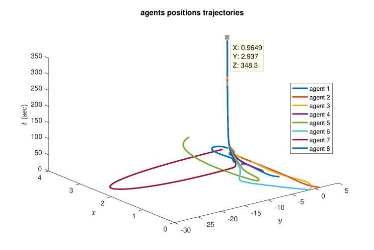
Figure 1: Position trajectories of double-integrator agents in numerical example.

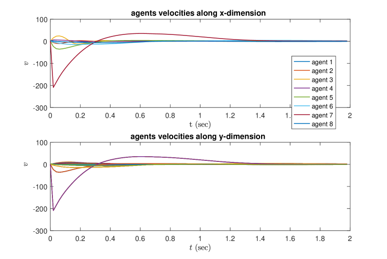
Figure 2: Velocity trajectories of double-integrator agents along both $x$ (down) and $y$ (top) dimension.

6 Conclusion

The problem of distributed constrained optimal consensus for undirected networks of dynamical agents was fully investigated in this paper. Here, all agents are supposed to rendezvous at a point that minimizes a collective convex objective function with regard to some local constraints. We studied this problem for two typical dynamics, namely single-integrator and double-integrator dynamics. To tackle the problem, we split it into two separate subproblems, viz consensus subproblem and distributed constrained convex optimization one. Then, we proposed a distributed control law composed of a consensus protocol and a term associated with decentralized convex optimization algorithm. In the proposed setup, each agent requires to know of its own states and the relative positions of agents within its neighborhood set. No information associated with objective functions are exchanged between agents.

To certify consensus, we exploited some theory associated with the analysis of perturbed systems stability. As for constrained convex optimization algorithm, we adopted an extended form of the interior-point method. Then, through Barbalat’s lemma, it was illustrated that optimality conditions, including the stationary condition and the feasibility condition, uniformly hold.

Finally, to relax the restricting assumption of local constraints being common, we exploited the distributed average tracking tool to estimate some essential information associated with the whole network at the local level. Then, we proved the convergence of our algorithm.

7 Appendix

In this appendix, we clarify how the inequality $\bar{v}^{\top}\Pi sig(\bar{v})^{p}\geq{\scriptstyle{\textstyle\frac{N-1}{N}}}\left(\left\|\bar{v}\right\|_{p+1}\right)^{p+1}$ holds for any $\bar{v}\in\mathbb{{R}}^{N}$.

$$\bar{v}^{\top}\Pi sig(\bar{v})^{p} =\bar{v}^{\top}\left[\begin{array}[]{cccc}\frac{N-1}{N}&-\frac{1}{N}&\cdots&-\frac{1}{N}\\ -\frac{1}{N}&\frac{N-1}{N}&\cdots&-\frac{1}{N}\\ \vdots&\vdots&\ddots&\vdots\\ -\frac{1}{N}&-\frac{1}{N}&\cdots&\frac{N-1}{N}\end{array}\right]sig(\bar{v})^{p}$$ (94)

$$={\scriptstyle{\textstyle\frac{N-1}{N}}}\sum_{i=1}^{N}\left|v_{i}\right|^{p+1}-{\textstyle{\textstyle\frac{1}{N}}}\sum_{i=1}^{N}\sum_{\underset{j\neq i}{j=1}}^{N}v_{j}\left|v_{i}\right|^{p}sign(v_{i})$$ (95)

$$\geq{\scriptstyle{\textstyle\frac{N-1}{N}}}\sum_{i=1}^{N}\left|v_{i}\right|^{p+1}-{\textstyle{\textstyle\frac{1}{N}}}\sum_{i=1}^{N}\sum_{\underset{j\neq i}{j=1}}^{N}\left|v_{j}\right|\left|v_{i}\right|^{p}$$ (96)

$$={\textstyle\frac{1}{N}\left|v_{1}\right|^{p}}\sum_{j=2}^{N}\left(\left|v_{1}\right|-\left|v_{j}\right|\right)$$

$$+{\textstyle\frac{1}{N}\left|v_{2}\right|^{p}}\sum_{\underset{j\neq 2}{j=1}}^{N}\left(\left|v_{2}\right|-\left|v_{j}\right|\right)+\cdots+{\textstyle\frac{1}{N}\left|v_{N}\right|^{p}}\sum_{\underset{j\neq N}{j=1}}^{N}\left(\left|v_{N}\right|-\left|v_{j}\right|\right)$$ (97)

$$=I$$ (98)

Now, assume that $\left|v_{i}\right|-\left|v_{j}\right|=\epsilon_{ij}$ for some $\epsilon_{ij}\in\mathbb{{R}}$. Then, we rewrite the left side of the equality (97) as

$$I=\frac{1}{2}\left({\textstyle\frac{1}{N}}\sum_{j=2}^{N}\epsilon_{1j}\left(\left|v_{1}\right|^{p}-\left|v_{j}\right|^{p}\right)+\cdots+{\textstyle\frac{1}{N}}\sum_{\underset{j\neq N}{j=1}}^{N}\epsilon_{Nj}\left(\left|v_{N}\right|^{p}-\left|v_{j}\right|^{p}\right)\right).$$ (99)

It is straightforward to show that $I\geq 0$, for any $\bar{v}\in\mathbb{{R}}^{N}$. Therefore, $\bar{v}^{\top}\Pi sig(\bar{v})^{p}\geq 0,\forall\bar{v}\in\mathbb{R}^{N}$. On the other hand, from (96), we have

$$\bar{v}^{\top}\Pi sig(\bar{v})^{p} \geq {\scriptstyle{\textstyle\frac{N-1}{N}}}\sum_{i=1}^{N}\left|v_{i}\right|^{p+1}$$ (100)

$$= {\scriptstyle{\textstyle\frac{N-1}{N}}}\left(\left\|\bar{v}\right\|_{p+1}\right)^{p+1}.$$

References

• Boyd \BBA Vandenberghe (\APACyear2004) \APACinsertmetastarboyd2004convex{APACrefauthors}Boyd, S.\BCBT \BBA Vandenberghe, L.  \APACrefYear2004. \APACrefbtitleConvex optimization Convex optimization. \APACaddressPublisherCambridge university press. \PrintBackRefs\CurrentBib
• Chen \BOthers. (\APACyear2012) \APACinsertmetastarchen2012distributed{APACrefauthors}Chen, F., Cao, Y.\BCBL \BBA Ren, W.  \APACrefYearMonthDay2012. \BBOQ\APACrefatitleDistributed average tracking of multiple time-varying reference signals with bounded derivatives Distributed average tracking of multiple time-varying reference signals with bounded derivatives.\BBCQ \APACjournalVolNumPagesIEEE Transactions on Automatic Control57123169–3174. \PrintBackRefs\CurrentBib
• Cheng \BOthers. (\APACyear2016) \APACinsertmetastarcheng2016reaching{APACrefauthors}Cheng, L., Wang, H., Hou, Z\BHBIG.\BCBL \BBA Tan, M.  \APACrefYearMonthDay2016. \BBOQ\APACrefatitleReaching a consensus in networks of high-order integral agents under switching directed topologies Reaching a consensus in networks of high-order integral agents under switching directed topologies.\BBCQ \APACjournalVolNumPagesInternational Journal of Systems Science4781966–1981. \PrintBackRefs\CurrentBib
• Fan \BOthers. (\APACyear2014) \APACinsertmetastarfan2014semi{APACrefauthors}Fan, M\BHBIC., Chen, Z.\BCBL \BBA Zhang, H\BHBIT.  \APACrefYearMonthDay2014. \BBOQ\APACrefatitleSemi-global consensus of nonlinear second-order multi-agent systems with measurement output feedback Semi-global consensus of nonlinear second-order multi-agent systems with measurement output feedback.\BBCQ \APACjournalVolNumPagesIEEE Transactions on Automatic Control5982222–2227. \PrintBackRefs\CurrentBib
• Fiacco \BBA McCormick (\APACyear1990) \APACinsertmetastarfiacco1990nonlinear{APACrefauthors}Fiacco, A\BPBIV.\BCBT \BBA McCormick, G\BPBIP.  \APACrefYear1990. \APACrefbtitleNonlinear programming: sequential unconstrained minimization techniques Nonlinear programming: sequential unconstrained minimization techniques (\BVOL 4). \APACaddressPublisherSiam. \PrintBackRefs\CurrentBib
• Horn \BBA Johnson (\APACyear2012) \APACinsertmetastarhorn2012matrix{APACrefauthors}Horn, R\BPBIA.\BCBT \BBA Johnson, C\BPBIR.  \APACrefYear2012. \APACrefbtitleMatrix analysis Matrix analysis. \APACaddressPublisherCambridge university press. \PrintBackRefs\CurrentBib
• Khalil (\APACyear1996) \APACinsertmetastarkhalil1996nonlinear{APACrefauthors}Khalil, H.  \APACrefYear1996. \APACrefbtitleNonlinear Systems Nonlinear systems. \APACaddressPublisherPrentice Hall. \PrintBackRefs\CurrentBib
• Kia \BOthers. (\APACyear2015) \APACinsertmetastarkia2015distributed{APACrefauthors}Kia, S\BPBIS., Cortés, J.\BCBL \BBA Martínez, S.  \APACrefYearMonthDay2015. \BBOQ\APACrefatitleDistributed convex optimization via continuous-time coordination algorithms with discrete-time communication Distributed convex optimization via continuous-time coordination algorithms with discrete-time communication.\BBCQ \APACjournalVolNumPagesAutomatica55254–264. \PrintBackRefs\CurrentBib
• Lee \BBA Mesbahi (\APACyear2011) \APACinsertmetastarlee2011constrained{APACrefauthors}Lee, U.\BCBT \BBA Mesbahi, M.  \APACrefYearMonthDay2011. \BBOQ\APACrefatitleConstrained consensus via logarithmic barrier functions Constrained consensus via logarithmic barrier functions.\BBCQ \BIn \APACrefbtitle2011 50th IEEE Conference on Decision and Control and European Control Conference 2011 50th ieee conference on decision and control and european control conference (\BPGS 3608–3613). \PrintBackRefs\CurrentBib
• Lin \BBA Ren (\APACyear2014) \APACinsertmetastarlin2014constrained{APACrefauthors}Lin, P.\BCBT \BBA Ren, W.  \APACrefYearMonthDay2014. \BBOQ\APACrefatitleConstrained consensus in unbalanced networks with communication delays Constrained consensus in unbalanced networks with communication delays.\BBCQ \APACjournalVolNumPagesIEEE Transactions on Automatic Control593775–781. \PrintBackRefs\CurrentBib
• Lu \BBA Tang (\APACyear2012) \APACinsertmetastarlu2012zero{APACrefauthors}Lu, J.\BCBT \BBA Tang, C\BPBIY.  \APACrefYearMonthDay2012. \BBOQ\APACrefatitleZero-gradient-sum algorithms for distributed convex optimization: The continuous-time case Zero-gradient-sum algorithms for distributed convex optimization: The continuous-time case.\BBCQ \APACjournalVolNumPagesIEEE Transactions on Automatic Control5792348–2354. \PrintBackRefs\CurrentBib
• Nedic \BBA Ozdaglar (\APACyear2009) \APACinsertmetastarnedic2009distributed{APACrefauthors}Nedic, A.\BCBT \BBA Ozdaglar, A.  \APACrefYearMonthDay2009. \BBOQ\APACrefatitleDistributed subgradient methods for multi-agent optimization Distributed subgradient methods for multi-agent optimization.\BBCQ \APACjournalVolNumPagesIEEE Transactions on Automatic Control54148–61. \PrintBackRefs\CurrentBib
• Nedic \BOthers. (\APACyear2010) \APACinsertmetastarnedic2010constrained{APACrefauthors}Nedic, A., Ozdaglar, A.\BCBL \BBA Parrilo, P\BPBIA.  \APACrefYearMonthDay2010. \BBOQ\APACrefatitleConstrained consensus and optimization in multi-agent networks Constrained consensus and optimization in multi-agent networks.\BBCQ \APACjournalVolNumPagesIEEE Transactions on Automatic Control554922–938. \PrintBackRefs\CurrentBib
• Olfati-Saber \BBA Murray (\APACyear2004) \APACinsertmetastarolfati2004consensus{APACrefauthors}Olfati-Saber, R.\BCBT \BBA Murray, R\BPBIM.  \APACrefYearMonthDay2004. \BBOQ\APACrefatitleConsensus problems in networks of agents with switching topology and time-delays Consensus problems in networks of agents with switching topology and time-delays.\BBCQ \APACjournalVolNumPagesIEEE Transactions on automatic control4991520–1533. \PrintBackRefs\CurrentBib
• Polycarpou \BBA Ioannou (\APACyear1993) \APACinsertmetastarpolycarpou1993robust{APACrefauthors}Polycarpou, M\BPBIM.\BCBT \BBA Ioannou, P\BPBIA.  \APACrefYearMonthDay1993. \BBOQ\APACrefatitleA robust adaptive nonlinear control design A robust adaptive nonlinear control design.\BBCQ \BIn \APACrefbtitleAmerican Control Conference, 1993 American control conference, 1993 (\BPGS 1365–1369). \PrintBackRefs\CurrentBib
• Qiu \BOthers. (\APACyear2016) \APACinsertmetastarqiu2016distributed{APACrefauthors}Qiu, Z., Liu, S.\BCBL \BBA Xie, L.  \APACrefYearMonthDay2016. \BBOQ\APACrefatitleDistributed constrained optimal consensus of multi-agent systems Distributed constrained optimal consensus of multi-agent systems.\BBCQ \APACjournalVolNumPagesAutomatica68209–215. \PrintBackRefs\CurrentBib
• Raffard \BOthers. (\APACyear2004) \APACinsertmetastarraffard2004distributed{APACrefauthors}Raffard, R\BPBIL., Tomlin, C\BPBIJ.\BCBL \BBA Boyd, S\BPBIP.  \APACrefYearMonthDay2004. \BBOQ\APACrefatitleDistributed optimization for cooperative agents: Application to formation flight Distributed optimization for cooperative agents: Application to formation flight.\BBCQ \BIn \APACrefbtitleDecision and Control, 2004. CDC. 43rd IEEE Conference on Decision and control, 2004. cdc. 43rd ieee conference on (\BVOL 3, \BPGS 2453–2459). \PrintBackRefs\CurrentBib
• Rahili \BBA Ren (\APACyear2017) \APACinsertmetastarrahili2015distributed{APACrefauthors}Rahili, S.\BCBT \BBA Ren, W.  \APACrefYearMonthDay2017. \BBOQ\APACrefatitleDistributed continuous-time convex optimization with time-varying cost functions Distributed continuous-time convex optimization with time-varying cost functions.\BBCQ \APACjournalVolNumPagesIEEE Transactions on Automatic Control6241590–1605. \PrintBackRefs\CurrentBib
• Ren \BBA Atkins (\APACyear2007) \APACinsertmetastarren2007distributed{APACrefauthors}Ren, W.\BCBT \BBA Atkins, E.  \APACrefYearMonthDay2007. \BBOQ\APACrefatitleDistributed multi-vehicle coordinated control via local information exchange Distributed multi-vehicle coordinated control via local information exchange.\BBCQ \APACjournalVolNumPagesInternational Journal of Robust and Nonlinear Control1710-111002–1033. \PrintBackRefs\CurrentBib
• Rezaee \BBA Abdollahi (\APACyear2015) \APACinsertmetastarrezaee2015average{APACrefauthors}Rezaee, H.\BCBT \BBA Abdollahi, F.  \APACrefYearMonthDay2015. \BBOQ\APACrefatitleAverage consensus over high-order multiagent systems Average consensus over high-order multiagent systems.\BBCQ \APACjournalVolNumPagesIEEE Transactions on Automatic Control60113047–3052. \PrintBackRefs\CurrentBib
• Tao (\APACyear1997) \APACinsertmetastartao1997simple{APACrefauthors}Tao, G.  \APACrefYearMonthDay1997. \BBOQ\APACrefatitleA simple alternative to the Barbalat lemma A simple alternative to the barbalat lemma.\BBCQ \APACjournalVolNumPagesIEEE Transactions on Automatic Control425698. \PrintBackRefs\CurrentBib
• J. Wang \BBA Elia (\APACyear2011) \APACinsertmetastarwang2011control{APACrefauthors}Wang, J.\BCBT \BBA Elia, N.  \APACrefYearMonthDay2011. \BBOQ\APACrefatitleA control perspective for centralized and distributed convex optimization A control perspective for centralized and distributed convex optimization.\BBCQ \BIn \APACrefbtitle2011 50th IEEE Conference on Decision and Control and European Control Conference 2011 50th ieee conference on decision and control and european control conference (\BPGS 3800–3805). \PrintBackRefs\CurrentBib
• X. Wang \BBA Hong (\APACyear2008) \APACinsertmetastarwang2008finite{APACrefauthors}Wang, X.\BCBT \BBA Hong, Y.  \APACrefYearMonthDay2008. \BBOQ\APACrefatitleFinite-time consensus for multi-agent networks with second-order agent dynamics Finite-time consensus for multi-agent networks with second-order agent dynamics.\BBCQ \APACjournalVolNumPagesIFAC Proceedings Volumes41215185–15190. \PrintBackRefs\CurrentBib
• Wieland \BOthers. (\APACyear2011) \APACinsertmetastarwieland2011internal{APACrefauthors}Wieland, P., Sepulchre, R.\BCBL \BBA Allgöwer, F.  \APACrefYearMonthDay2011. \BBOQ\APACrefatitleAn internal model principle is necessary and sufficient for linear output synchronization An internal model principle is necessary and sufficient for linear output synchronization.\BBCQ \APACjournalVolNumPagesAutomatica4751068–1074. \PrintBackRefs\CurrentBib
• Xie \BBA Lin (\APACyear2017) \APACinsertmetastarxie2017global{APACrefauthors}Xie, Y.\BCBT \BBA Lin, Z.  \APACrefYearMonthDay2017. \BBOQ\APACrefatitleGlobal optimal consensus for multi-agent systems with bounded controls Global optimal consensus for multi-agent systems with bounded controls.\BBCQ \APACjournalVolNumPagesSystems & Control Letters102104–111. \PrintBackRefs\CurrentBib
• Yang \BOthers. (\APACyear2016) \APACinsertmetastaryang2016multi{APACrefauthors}Yang, S., Liu, Q.\BCBL \BBA Wang, J.  \APACrefYearMonthDay2016. \BBOQ\APACrefatitleA multi-agent system with a proportional-integral protocol for distributed constrained optimization A multi-agent system with a proportional-integral protocol for distributed constrained optimization.\BBCQ \APACjournalVolNumPagesIEEE Transactions on Automatic Control. \PrintBackRefs\CurrentBib
• Yi \BOthers. (\APACyear2015) \APACinsertmetastaryi2015distributed{APACrefauthors}Yi, P., Hong, Y.\BCBL \BBA Liu, F.  \APACrefYearMonthDay2015. \BBOQ\APACrefatitleDistributed gradient algorithm for constrained optimization with application to load sharing in power systems Distributed gradient algorithm for constrained optimization with application to load sharing in power systems.\BBCQ \APACjournalVolNumPagesSystems & Control Letters8345–52. \PrintBackRefs\CurrentBib
• Yuan \BOthers. (\APACyear2011) \APACinsertmetastaryuan2011distributed{APACrefauthors}Yuan, D., Xu, S.\BCBL \BBA Zhao, H.  \APACrefYearMonthDay2011. \BBOQ\APACrefatitleDistributed primal–dual subgradient method for multiagent optimization via consensus algorithms Distributed primal–dual subgradient method for multiagent optimization via consensus algorithms.\BBCQ \APACjournalVolNumPagesIEEE Transactions on Systems, Man, and Cybernetics, Part B (Cybernetics)4161715–1724. \PrintBackRefs\CurrentBib
• Zhang \BBA Lewis (\APACyear2012) \APACinsertmetastarzhang2012adaptive{APACrefauthors}Zhang, H.\BCBT \BBA Lewis, F\BPBIL.  \APACrefYearMonthDay2012. \BBOQ\APACrefatitleAdaptive cooperative tracking control of higher-order nonlinear systems with unknown dynamics Adaptive cooperative tracking control of higher-order nonlinear systems with unknown dynamics.\BBCQ \APACjournalVolNumPagesAutomatica4871432–1439. \PrintBackRefs\CurrentBib