Bounds on the Entropy of a Function of a Random Variable and their Applications

Abstract

It is well known that the entropy $H(X)$ of a discrete random variable $X$ is always greater than or equal to the entropy $H(f(X))$ of a function $f$ of $X$, with equality if and only if $f$ is one-to-one. In this paper, we give tight bounds on $H(f(X))$ when the function $f$ is not one-to-one, and we illustrate a few scenarios where this matters. As an intermediate step towards our main result, we derive a lower bound on the entropy of a probability distribution, when only a bound on the ratio between the maximal and minimal probabilities is known. The lower bound improves on previous results in the literature, and it could find applications outside the present scenario.

I The Problem

Let $\mathcal{X}=\{x_{1},\ldots,x_{n}\}$ be a finite alphabet, and $X$ be any random variable (r.v.) taking values in $\mathcal{X}$ according to the probability distribution ${\bf p}=(p_{1},p_{2},\ldots,p_{n})$, that is, such that $P\{X=x_{i}\}=p_{i}$, for $i=1,2,\ldots,n$. A well known and widely used inequality states that

$$H(f(X))\leq H(X),$$ (1)

where $f\colon\mathcal{X}\to\mathcal{Y}$ is any function defined on $\mathcal{X}$, and $H(\cdot)$ denotes the Shannon entropy. Moreover, equality holds in (1) if and only if the function $f$ is one-to-one. The main purpose of this paper is to sharpen inequality (1) by deriving tight bounds on $H(f(X))$ when $f$ is not one-to-one. More precisely, given the r.v. $X$, an integer $2\leq m<n$, a set $\mathcal{Y}_{m}=\{y_{1},\ldots,y_{m}\}$, and the family of surjective functions $\mathcal{F}_{m}=\{f|\;f\colon\mathcal{X}\to\mathcal{Y}_{m},\ |f(\mathcal{X})|=m\}$, we want to compute the values

$$\max_{f\in\mathcal{F}_{m}}H(f(X))\qquad\mbox{and}\qquad\min_{f\in\mathcal{F}_{m}}H(f(X)).$$ (2)

While computing the $\min_{f\in\mathcal{F}_{m}}H(f(X))$ is easy, the computation of $\max_{f\in\mathcal{F}_{m}}H(f(X))$ turns out to be a challenging, but otherwise consequential, problem. It is also worth noticing that maximizing $H(f(X))$ for random functions is trivial, since the value $\log m$ is always achievable.

II The Results

For any probability distribution ${\bf p}=(p_{1},p_{2},\ldots,p_{n})$, with $p_{1}\geq p_{2},\ldots,\geq p_{n}\geq 0$, and integer $2\leq m<n$, let us define the probability distributions $R_{m}({\bf p})=(r_{1},\ldots,r_{m})$ as follows: if $p_{1}<1/m$ we set $R_{m}({\bf p})=(1/m,\ldots,1/m)$, whereas if $p_{1}\geq 1/m$ we set $R_{m}({\bf p})=(r_{1},\ldots,r_{m})$, where

$$r_{i}=\begin{cases}p_{i}&\hbox{ for }i=1,\dots,i^{*}\cr\left(\sum_{j=i^{*}+1}^{n}p_{j}\right)/{(m-i^{*})}&\hbox{ for }i=i^{*}+1,\dots,m,\end{cases}$$ (3)

and $i^{*}$ is the maximum index $i$ such that $p_{i}\geq\frac{\sum_{j=i+1}^{n}p_{j}}{m-i}$. A somewhat similar operator was introduced in [19].

As suggested by one of the referees, the operator $R_{m}({\bf p})$ can also be explained in the following way. For a given r.v. $X$ distributed in the alphabet $\mathcal{X}$ according to ${\bf p}$, the alphabet $\mathcal{X}$ can be partitioned in two sets $\mathcal{X}_{\mbox{\footnotesize large}}=\{x_{1},\ldots,x_{i^{*}}\}$ and $\mathcal{X}_{\mbox{\footnotesize small}}=\mathcal{X}\setminus\mathcal{X}_{\mbox{\footnotesize large}}$. Now, a r.v. $\hat{X}$ can be defined to be distributed just like $X$ conditioned on the event that $X\in\mathcal{X}_{\mbox{\footnotesize large}}$, and uniformly over $\mathcal{X}_{\mbox{\footnotesize small}}$, conditioned on the event that $X\in\mathcal{X}_{\mbox{\footnotesize small}}$. When the integer $i^{*}$ is chosen to be the largest possible that ensures that the probability distribution of $\hat{X}$ remains ordered, then the probability distribution of $\hat{X}$ is exactly $R_{m}({\bf p})$.

We also define the probability distributions $Q_{m}({\bf p})=(q_{1},\ldots,q_{m})$ in the following way:

$$q_{i}=\begin{cases}\sum_{k=1}^{n-m+1}p_{k},\quad&\hbox{ for }i=1,\cr p_{n-m+i},&\hbox{ for }i=2,\ldots,m.\end{cases}$$ (4)

The following Theorem provides the results seeked in (2).

Theorem 1.

For any r.v. $X$ taking values in the alphabet $\mathcal{X}=\{x_{1},x_{2},\ldots,x_{n}\}$ according to the probability distribution ${\bf p}=(p_{1},p_{2},\ldots,p_{n})$, and for any $2\leq m<n$, it holds that

$$\max_{f\in\mathcal{F}_{m}}H(f(X))\in\left[H(R_{m}({\bf p}))-\alpha,H(R_{m}({\bf p}))\right],$$ (5)

where $\alpha=1-({1+\ln(\ln 2)})/{\ln 2}<0.08608$, and

$$\min_{f\in\mathcal{F}_{m}}H(f(X))=H(Q_{m}({\bf p})).$$ (6)

Here, with a slight abuse of notation, for a probability distribution ${\bf a}=(a_{1},\ldots,a_{t})$ we denote with $H({\bf a})=-\sum_{i}a_{i}\log a_{i}$ the entropy of a discrete r.v. distributed according to ${\bf a}$. Moreover, with $\log$ we denote the logarithm in base 2, and with $\ln$ the natural logarithm in base $e$.

Therefore, according to Theorem 1, the function $f\in\mathcal{F}_{m}$ for which $H(f(X))$ is minimum maps all the elements $x_{1},\ldots,x_{n-m+1}\in\mathcal{X}$ to a single element, and it is one-to-one on the remaining elements $x_{n-m+2},\ldots,x_{n}$.

Before proving Theorem 1 and discuss its consequences, we would like to notice that there are quite compelling reasons why we are unable to determine the exact value of the maximum in (5), and consequently, the form of the function $f\in\mathcal{F}_{m}$ that attains the bound. Indeed, computing the value $\max_{f\in\mathcal{F}_{m}}H(f(X))$ is an NP-hard problem. It is easy to understand the difficulty of the problem already in the simple case $m=2$. To that purpose, consider any function $f\in\mathcal{F}_{2}$, that is $f\colon\mathcal{X}\to\mathcal{Y}_{2}=\{y_{1},y_{2}\}$, and let $X$ be any r.v. taking values in $\mathcal{X}$ according to the probability distribution ${\bf p}=(p_{1},p_{2},\ldots,p_{n})$. Let $\sigma_{1}=\!\!\!\sum_{x\in\mathcal{X}:f(x)=y_{1}}P\{X=x\},\quad\sigma_{2}=\!\!\!\sum_{x\in\mathcal{X}:f(x)=y_{2}}P\{X=x\}.$ Then,

$$H(f(X))=-\sigma_{1}\log\sigma_{1}-\sigma_{2}\log\sigma_{2},$$

and it is maximal in correspondence of a function $f\in\mathcal{F}_{2}$ that makes the sums $\sigma_{1}$ and $\sigma_{2}$ as much equal as possible. This is equivalent to the well known NP-hard problem Partition on the instance $\{p_{1},\ldots,p_{n}\}$ (see [17]). Actually, we can prove a stronger result. We first recall that problem is said to be strongly NP-hard if it is NP-hard even when all of its numerical parameters are bounded by a polynomial in the length of the input [17]. More importantly, any strongly NP-hard optimization problem with a polynomially bounded objective function cannot have a fully polynomial-time approximation scheme unless $P=NP$ [17].

Lemma 1.

The problem of computing $\max_{f\in\mathcal{F}_{m}}H(f(X))$ is strongly NP-hard.

Proof:

The following reduction from the well known 3-Partition problem [42] proves the result. We recall that in the 3-Partition problem we are given a set of $N=3m$ numbers $A=\{a_{1},\dots,a_{N}\}$, with $\sum_{i}a_{i}=mB$, and such that each number $a_{i}$ satisfies $\frac{B}{4}<a_{i}<\frac{B}{2}.$ The question is to decide whether it is possible to partition $A$ into subsets $A_{1},\ldots,A_{m}$, such that $|A_{j}|=3$ and $\sum_{a\in A_{j}}a=B$, for each $j=1,\ldots m.$ This problem is known to be strongly NP-complete (see [42], Theorem 7.2.4).

We will reduce 3-Partition to our problem: Let $A$ be an instance of 3-Partition, and $N,m$ and $B$ be as above. Let $X$ be a random variable taking values in $\{1,\ldots,N\}=[N]$, distributed according to ${\bf p}=(p_{1},\dots,p_{N})$, where $p_{i}=a_{i}/(mB)$, for $i=1,\ldots,N$. Assume first that there exists a partition $A_{1},\dots,A_{m}$ of the set $A$ such that for each $j=1,\dots,m,$ we have $|A_{j}|=3$ and $\sum_{a\in A_{j}}a=B$. Let $f$ be the function $f\colon[N]\mapsto\{1,\ldots,m\}=[m]$ defined by stipulating that $f(i)=j$ if and only if $a_{i}\in A_{j}$. It is easy to see that $H(f(X))=\log m.$

Conversely, let $f\colon[N]\mapsto[m]$ be a function such that $H(f(X))=\log m.$ This implies that the random variable $f(X)$ is equiprobable, i.e., for each $y\in[m]$ we have that

$$\sum_{i\in[N]\;:\;f(i)=y}p_{i}=\frac{1}{m}.$$

Let $B_{y}=\{i\in[N]\,:\,f(i)=y\}.$ Since, by definition, we have $\frac{1}{4m}<p_{i}<\frac{1}{2m},$ we have that for each $y$ it must hold $|B_{y}|=3.$ Moreover, we have $\sum_{i\in B_{y}}a_{i}=Bm\sum_{i\in B_{y}}p_{i}=B.$ Hence, letting $A_{y}=\{a_{i}\in A\mid f(i)=y\}$ we have that $A_{1},\dots,A_{m}$ is a partition of $A$ into sets of size $3$ with equal total sum. Therefore, we can map any instance of 3-Partition into an instance of our problem such that there exists a function $f\colon[N]\mapsto[m]$ with $H(f(X))=\log m$ if and only if the $3$-Partition instance admits the desired partition. ∎

In this paper we will also show that the function $f\in\mathcal{F}_{m}$ for which $H(f(X))\geq H(R_{m}({\bf p}))-\alpha$ can be efficiently determined, therefore we also have the following important consequence of Theorem 1.

Corollary 1.

There is a polynomial time algorithm to approximate the NP-hard problem of computing the value

$$\max_{f\in\mathcal{F}_{m}}H(f(X)),$$

with an additive approximation factor not greater than $1-({1+\ln(\ln 2)})/{\ln 2}<0.08608$.

Under the plausible assumption that $P\neq NP$, the strong NP-hardness result proved in Lemma 1 rules out the existence of polynomial time algorithms that, for any values of $\epsilon>0$, compute a function $g\in\mathcal{F}_{m}$ such that $H(g(X))\geq(1-\epsilon)\max_{f\in\mathcal{F}_{m}}H(f(X))$. Therefore, we find it quite interesting that the problem in question admits the approximation algorithm with the small additive error mentioned in Corollary 1, since only a handful NP-hard optimization problems are known to enjoy this property. In Section IV-A we will also prove that the polynomial time algorithm referred to in Corollary 1 outputs a solution whose value is at least $\frac{10}{11}\Bigl{(}\max_{f\in\mathcal{F}_{m}}H(f(X))\Bigr{)}$.

A key tool for the proof of Theorem 1 is the following result, proved in Section V.

Theorem 2.

Let ${\bf p}=(p_{1},p_{2},\ldots,p_{n})$ be a probability distribution such that $p_{1}\geq p_{2}\geq\ldots\geq p_{n}>0$. If $p_{1}/p_{n}\leq{\rho}$ then

$$H({\bf p})\geq\log n-\left(\frac{{\rho}\ln{\rho}}{{\rho}-1}-1-\ln\frac{{\rho}\ln{\rho}}{{\rho}-1}\right)\frac{1}{\ln 2}.$$ (7)

Theorem 2 improves on several papers (see [37] and references therein), that have studied the problem of estimating $H({\bf p})$ when only a bound on the ratio $p_{1}/p_{n}$ is known. Moreover, besides its application in the proof of the lower bound in (5), Theorem 2 has consequences of independent interest. In particular, in Section VI we will show how Theorem 2 allows us to provide a new upper bound on the compression rate of Tunstall codes for discrete memoryless and stationary sources. Our new bound improves the classical result of Jelinek and Schneider [21].

To prove our results, we use ideas and techniques from majorization theory [31], a mathematical framework that has been proved to be very much useful in information theory (e.g., see [3, 4, 19, 20] and references therein).

III Some Applications

Besides its inherent naturalness, the problem of estimating the entropy $H(f(X))$ has several interesting consequences. We highlight some of them here.

III-A Clustering

In the area of clustering [16], one seeks a mapping $f$ (either deterministic or stochastic) from some data, generated by a r.v. $X$ taking values in a set $\mathcal{X}$, to “labels” in some set $\mathcal{Y}$, where typically $|\mathcal{Y}|\ll|\mathcal{X}|$. Clusters are subsets $C\subseteq\mathcal{X}$ whose elements are mapped to a same label $y\in\mathcal{Y}$. A widely employed measure to appraise the goodness of a clustering algorithm is the information that the clusters retain towards the original data, measured by the mutual information $I(X;f(X))$ (see [15, 23] and references therein). In general, one wants to choose $f$ such that $|f(\mathcal{X})|$ is small but $I(X;f(X))$ is large. The authors of [18] (see also [25]) proved that, given the random variable $X$, among all mappings $f$ that maximizes $I(X;f(X))$ (under the constraint that the cardinality $|f(\mathcal{X})|$ is fixed) there is a maximizing function $f$ that is deterministic. This is essentially a consequence of the fact that the mutual information is convex in the conditional probabilities. Since in the case of deterministic functions it holds that $I(X;f(X))=H(f(X))$, it is obvious that finding the clustering $f$ of $\mathcal{X}$ (into a fixed number $m$ of clusters) that maximizes the mutual information $I(X;f(X))$ is equivalent to our problem of finding the function $f$ that appears in Corollary 1. We also remark that the problem of determining the function $f$ that maximizes the mutual information $I(X;f(X))$ (under the constraint that the cardinality $|f(\mathcal{X})|$ is fixed) has also been posed in [12, 13]. Other work that considers the general problem of reducing the alphabet size of a random variable $X$, while trying to preserve the information that it gives towards another random variable $Y$, is contained in [26, 22]. Our work seems also related to the well known information bottleneck method [40], mainly in the “agglomerative” or “deterministic” version, see [38, 39]. This connections will be explored elsewhere.

III-B Approximating probability distributions with low dimensional ones

Another scenario where our results directly find applications is the one considered in [41]. There, the author considers the problem of best approximating a probability distribution ${\bf p}=(p_{1},\ldots,p_{n})$ with a lower dimensional one ${\bf q}^{*}=(q^{*}_{1},\ldots,q^{*}_{m})$, $m\leq n$. The criterion with which one chooses ${\bf q}^{*}$, given ${\bf p}$, is the following. Given arbitrary ${\bf p}=(p_{1},\ldots,p_{n})$ and ${\bf q}=(q_{1},\ldots,q_{m})$, $m\leq n$, define the quantity ${\tt D}({\bf p},{\bf q})$ as $2W({\bf p},{\bf q})-H({\bf p})-H({\bf q})$, where $W({\bf p},{\bf q})$ is the minimum entropy of a bivariate probability distribution that has ${\bf p}$ and ${\bf q}$ as marginals. Equivalently, see [41, (9)] ${\tt D}({\bf p},{\bf q})=\min\bigl{\{}H(X|Y)+H(Y|X)\bigr{\}}$, where the minimization is with respect to all joint probability distributions of $X$ and $Y$ such that the random variable $X$ is distributed according to ${\bf p}$ and the random variable $Y$ according to ${\bf q}$. A joint probability distributions of $X$ and $Y$ such that the random variable $X$ is distributed according to a fixed ${\bf p}$ and the random variable $Y$ according to a fixed ${\bf q}$ is usually called a coupling of $X$ and $Y$. Couplings (with additional properties) play an important role in information theory questions, e.g., [35].

Having so defined the function ${\tt D}$, the “best” approximation ${\bf q}^{*}$ of ${\bf p}$ is chosen as the probability distributions ${\bf q}^{*}$ with $m$ components that minimizes ${\tt D}({\bf p},{\bf q})$, where the minimization is performed over all probability distributions ${\bf q}=(q_{1},\ldots,q_{m})$. The author of [41] motivates this choice, shows that the function ${\tt D}(\cdot,\cdot)$ is a pseudo distance among probability distributions, and proves that ${\bf q}^{*}$ can be characterized in the following way. Given ${\bf p}=(p_{1},\ldots,p_{n})$, call ${\bf q}=(q_{1},\ldots,q_{m})$ an aggregation of ${\bf p}$ into $m<n$ components if there is a partition of $\{1,\ldots,n\}$ into disjoint sets $I_{1},\ldots,I_{m}$ such that $q_{k}=\sum_{i\in I_{k}}p_{i}$, for $k=1,\ldots m$. In [41] it is proved that the vector ${\bf q}^{*}$ that best approximate ${\bf p}$ (according to ${\tt D}$) is the aggregation of ${\bf p}$ into $m$ components of maximum entropy. We notice that any aggregation ${\bf q}$ of ${\bf p}$ can be seen as the distribution of the r.v. $f(X)$, where $f$ is some appropriate non-injective function and $X$ is a r.v. distributed according to ${\bf p}$ (and, vice versa, any deterministic non-injective $f$ gives a r.v. $f(X)$ whose distribution is an aggregation of the distribution of the r.v. $X$). Therefore, from Lemma 1 one gets that the problem of computing the “best” approximation ${\bf q}^{*}$ of ${\bf p}$ is strongly NP-hard. The author of [41] proposes greedy algorithms to compute sub-optimal solutions both to the problem of computing the aggregation of ${\bf p}$ into $m$ components of maximum entropy and to the problem of computing the probability distributions ${\bf q}^{*}$ with $m$ components that minimizes ${\tt D}({\bf p},{\bf q})$. Notice, however, that no performance guarantee is given in [41] for the aforesaid greedy algorithms. In Section VII we will show how the bound (5) allows us to provide an approximation algorithm to construct a probability distribution $\overline{{\bf q}}=(\overline{q}_{1},\ldots,\overline{q}_{m})$ such that ${\tt D}({\bf p},\overline{{\bf q}})\leq{\tt D}({\bf p},{\bf q}^{*})+0.08608$, considerably improving on the result we presented in [7], where an approximation algorithm for the same problem with an additive error of $1$ was provided.

III-C Additional relations

There are other problems that can be cast in our scenario. For instance, Baez et al. [1] give an axiomatic characterization of the Shannon entropy in terms of information loss. Stripping away the Category Theory language of [1], the information loss of a r.v. $X$ amounts to the difference $H(X)-H(f(X))$, where $f$ is any deterministic function. Our Theorem 1 allows to quantify the extreme value of the information loss of a r.v., when the support of $f(X)$ is known.

In the paper [9] the authors consider the problem of constructing the best summary tree of a given weighted tree, by means of some contractions operations on trees. Two type of contractions are allowed: 1) subtrees may be contracted to single node that represent the corresponding subtrees, 2) multiple sibling subtrees (i.e., subtrees whose roots are siblings) may be contracted to single nodes representing them. Nodes obtained by contracting subtrees have weight equal to the sum of the node weights in the original contracted subtrees. Given a bound on the number of nodes in the resulting summary tree, the problem studied in [9] is to compute the summary tree of maximum entropy, where the entropy of a tree is the Shannon entropy of the normalized node weights. This is a particular case of our problem, when the function $f$ is not arbitrary but has to satisfy the constraints dictated by the allowed contractions operations on trees.

Another related paper is [14], where the authors consider a problem similar to ours, but now $f$ is restricted to be a low-degree polynomial and ${\bf p}$ is the uniform distribution.

There is also a vast literature (see [30], Section 3.3, and references therein) studying the “leakage of a program $P$ […] defined as the (Shannon) entropy of the partition $\Pi(P)$” [30]. One can easily see that their “leakage” is the same as the entropy $H(f(X))$, where $X$ is the r.v. modeling the program input, and $f$ is the function describing the input-output relation of the program $P$. In Section 8 of the same paper the authors study the problem of maximizing or minimizing the leakage, in the case the program $P$ is stochastic, using standard techniques based on Lagrange multipliers. They do not consider the (harder) case of deterministic programs (i.e., deterministic $f$’s) and our results are likely to be relevant in that context.

Our results are also related to Rota’s entropy-partition theory [27, 28]. Given a ground set $S=\{1,2,\ldots,n\}$, and a partition $\Pi=(C_{1},\ldots,C_{m})$ into $m$ classes of $S$, the entropy $H(\Pi)$ of $\Pi$ is defined as $H(\Pi)=\sum_{i=1}^{m}\frac{|C_{i}|}{n}\log\frac{n}{|C_{i}|}$. Rota was interested in the decrease (resp. increase) of the entropy of a partition under the operation of coarsening (resp., refining) of a partition, where two or more classes of the partition $\Pi$ are fused into a single class (resp., a class is split into two or more new classes). One can see that the decrease of $H(\Pi)$ due to the coarsening operation, for example, can be quantified by computing the entropy of $H(f(X))$, where $X$ is a r.v. distributed according to $\left(\frac{|C_{1}|}{n},\ldots,\frac{|C_{m}|}{n}\right)$, and $f$ is an appropriate function.

Our problem can also be seen as a problem of quantizing the alphabet of a discrete source into a smaller one (e.g., [33]), and the goal is to maximize the mutual information between the original source and the quantized one. Our results have also relations with those of [29], where it is considered the problems of aggregating data with a minimal information loss.

IV The Proof of Theorem 1

We first recall the important concept of majorization among probability distributions.

Definition 1.

[31] Given two probability distributions ${\bf a}=(a_{1},\ldots,a_{n})$ and ${\bf b}=(b_{1},\ldots,b_{n})$ with $a_{1}\geq\ldots\geq a_{n}\geq 0$ and $b_{1}\geq\ldots\geq b_{n}\geq 0$, we say that ${\bf a}$ is majorized by ${\bf b}$, and write ${\bf a}\preceq{\bf b}$, if and only if

$$\sum_{k=1}^{i}a_{k}\leq\sum_{k=1}^{i}b_{k},\quad\mbox{\rm for all }\ i=1,\ldots,n.$$

We will make extensive use of the Schur concavity of the entropy function $H$ (see [31], p. 101) that says:

$$H({\bf a})\geq H({\bf b}),\quad\mbox{ whenever }{\bf a}\preceq{\bf b}.$$ (8)

An important improvement of inequality (8) was proved in the paper [20], stating that

$$H({\bf a})\geq H({\bf b})+D({\bf b}||{\bf a}),$$ (9)

whenever ${\bf a},{\bf b}$ have been ordered and ${\bf a}\preceq{\bf b}$. Here $D({\bf b}||{\bf a})=\sum b_{i}\log(b_{i}/a_{i})$ is the relative entropy between ${\bf b}$ and ${\bf a}$. However, for most of our purposes the inequality (8) will be sufficient.

One can also extend the majorization relation to the set of all vectors of finite length by padding the shorter vector with zeros and applying Definition 1. This is customarily done in the literature (e.g., [34]). We also notice that this trick does not effect our results that uses (8), since adding zeros to a probability distribution ${\bf a}$ does not change the entropy value $H({\bf a})$.

The idea to prove Theorem 1 is simple. We shall first prove that for any function $f\in\mathcal{F}_{m}$, $m<n$, and for any r.v. $X$ distributed according to ${\bf p}=(p_{1},\ldots,p_{n})$, it holds that ${\bf p}$ is majorized by the probability distribution of the random variable $f(X)$. Successively, we will prove that the probability distribution $R_{m}({\bf p})$ defined in (3) is majorized by any ${\bf q}=(q_{1},\ldots,q_{m})$ such that ${\bf p}\preceq{\bf q}$ (in particular, by the the probability distribution of the random variable $f(X)$, with $f\in\mathcal{F}_{m}$). These facts, together with the Schur concavity of the entropy function will prove the upper bound $\max_{f\in\mathcal{F}_{m}}H(f(X))\leq H(R_{m}({\bf p}))$ in (5). We prove the lower bound in (5) by explicitly constructing a function $g\in\mathcal{F}_{m}$ such that $H(g(X))\geq H(R_{m}({\bf p}))-\alpha.$

Without loss of generality we assume that all the probabilities distributions we deal with have been ordered in non-increasing order. Since we will be working with functions of probability distributions that are invariant with respect to permutations of the variables, i.e., the Shannon entropy $H(\cdot)$, this is not a restriction. We also use the majorization relationship between vectors of unequal lengths, by properly padding the shorter one with the appropriate number of $0$’s at the end. The well known assumption that $0\log\frac{1}{0}=0$ allows us to do that.

Consider an arbitrary function $f\colon\mathcal{X}\to\mathcal{Y}$, $f\in\mathcal{F}_{m}$. Any r.v. $X$ taking values in $\mathcal{X}=\{x_{1},\ldots,x_{n}\}$, according to the probability distribution ${\bf p}=(p_{1},\ldots,p_{n})$, together with the function $f$, naturally induce a r.v. $f(X)$, taking values in $\mathcal{Y}=\{y_{1},\ldots,y_{m}\}$ according to the probability distribution whose values are given by the expressions

$$\forall y_{j}\in\mathcal{Y}\qquad P\{f(X)=y_{j}\}=\sum_{x\in\mathcal{X}:f(x)=y_{j}}P\{X=x\}.$$ (10)

Let ${\bf z}=(z_{1},\ldots,z_{m})$ be the vector containing the values $z_{1}=P\{f(X)=y_{1}\},\ldots,z_{m}=P\{f(X)=y_{m}\}$ ordered in non-increasing fashion. For convenience, we state the following self-evident fact about the relationships between ${\bf z}$ and ${\bf p}$.

Claim 1.

There is a partition of $\{1,\ldots,n\}$ into disjoint sets $I_{1},\ldots,I_{m}$ such that $z_{j}=\sum_{i\in I_{j}}p_{i}$, for $j=1,\ldots m$.

We will call such a ${\bf z}$ an aggregation of ${\bf p}$. In the paper [10] the authors use the different terminology of lumping, our nomenclature is taken from [41]. Given a r.v. $X$ distributed according to ${\bf p}$, and any function $f\in\mathcal{F}_{m}$, by simply applying the definition of majorization one can see that the (ordered) probability distribution of the r.v. $f(X)$ is majorized by $Q_{m}({\bf p})=(q_{1},\ldots,q_{m})$, as defined in (4). Therefore, by invoking the Schur concavity of the entropy function $H$ we get that $H(f(X))\geq H(Q_{m}({\bf p}))$. From this, the equality (6) immediately follows.

Denote by

$${\cal P}_{n}=\{{\bf p}=(p_{1},\ldots,p_{n})\in\mathbb{R}^{n}:p_{1}\geq\ldots p_{n}\geq 0,\sum_{i}p_{i}=1\}$$

the $(n-1)$-dimensional simplex. We need the following preliminary results.

Lemma 2.

For any ${\bf p}\in{\cal P}_{n}$, $m<n$, it holds that

$${\bf p}\preceq R_{m}({\bf p}).$$ (11)

Proof:

According to Definition 1, we need to prove that

$$\sum_{k=1}^{i}p_{k}\leq\sum_{k=1}^{i}r_{k},\mbox{ for }i=1,\ldots,m.$$ (12)

By the definition (3) of $R_{m}({\bf p})$, inequalities (12) are trivially true for each $i\leq i^{*}$. Moreover, by the definition of $i^{*}$ as the largest index $i$ for which $p_{i}\geq({\sum_{j=i+1}^{n}p_{j}})/({m-i})$ holds, one has $p_{i^{*}+1}<({\sum_{j=i^{*}+2}^{n}p_{j}})/({m-i^{*}-1})$. Summing up $p_{i^{*}+1}/(m-i^{*}-1)$ to both sides of the previous inequality, one has

$$\frac{\sum_{j=i^{*}+1}^{n}p_{j}}{m-i^{*}-1}>p_{i^{*}+1}+\frac{p_{i^{*}+1}}{m-i^{*}-1}=p_{i^{*}+1}\cdot\frac{m-i^{*}}{m-i^{*}-1}.$$

Therefore, $p_{i^{*}+1}<({\sum_{j=i^{*}+1}^{n}p_{j}})/({m-i^{*}})=r_{i^{*}+1}$. Since ${\bf p}$ has its components ordered in non increasing order, one has $p_{i}\leq r_{i}=r_{i^{*}+1}$ also for $i=i^{*}+1,\ldots,m$.

In conclusion, since we have proved that $p_{i}\leq r_{i}$, for all $i=1,\ldots,m$, and we also know that $\sum_{k=1}^{m}r_{k}=1$, we get that (12) is proved. ∎

Lemma 3.

Let ${\bf p}\in{\cal P}_{n}$, $m<n$, and ${\bf q}\in{\cal P}_{m}$ be any aggregation of ${\bf p}$. Then ${\bf p}\preceq{\bf q}$.

Proof:

We prove by induction on $i$ that $\sum_{k=1}^{i}q_{k}\geq\sum_{k=1}^{i}p_{k}$.
Since ${\bf q}=(q_{1},\ldots,q_{m})$ is an aggregation of ${\bf p}=(p_{1},\ldots,p_{n})$, one gets that there is a partition $I_{1},\dots,I_{m}$ of $\{1,\ldots,n\}$ such that $q_{i}=\sum_{j\in I_{i}}p_{j}$ for each $i=1,\dots,m.$ In particular, there exists a subset $I_{j}\subseteq\{1,\ldots,n\}$ such that $1\in I_{j}$. We then have $q_{1}\geq q_{j}\geq p_{1}$. Suppose now that $\sum_{k=1}^{i-1}q_{k}\geq\sum_{k=1}^{i-1}p_{k}$. If there exist indices $j\geq i$ and $\ell\leq i$ such that $\ell\in I_{j}$, then $q_{i}\geq q_{j}\geq p_{\ell}\geq p_{i}$, that implies $\sum_{k=1}^{i}q_{k}\geq\sum_{k=1}^{i}p_{k}$. Otherwise, for each $j\geq i$ and $\ell\leq i$ it holds that $\ell\not\in I_{j}$. Therefore, $\{1,\ldots,i\}\subseteq I_{1}\cup\ldots\cup I_{i-1}$. This immediately implies that $\sum_{k=1}^{i-1}q_{k}\geq\sum_{k=1}^{i}p_{k}$, from which we obviously get $\sum_{k=1}^{i}q_{k}\geq\sum_{k=1}^{i}p_{k}$. ∎

In other words, for any r.v. $X$ and function $f$, the probability distribution of $f(X)$ is an aggregation of the probability distribution of $X$. Therefore, the probability distribution of $f(X)$ always majorizes that of $X$. As a first consequence, from (9) we get that

$$H(X)\geq H(f(X))+D({\bf q}||{\bf p}),$$ (13)

where ${\bf p}$ is the probability distribution of $X$ and ${\bf q}$ is the probability distribution of $f(X)$. This is an improvement of the inequality $H(X)\geq H(f(X))$ that might be of independent interest. We highlight the inequality (13) in the following essentially equivalent formulation.

Corollary 2.

Let $X$ and $Y$ be arbitrary r.v., distributed according to ${\bf p}$ and ${\bf q}$, respectively. Then, if $H(Y|X)=0$ holds, one has that

$$H(X)\geq H(Y)+D({\bf q}||{\bf p}).$$

Next Lemma proves that, among all probability distributions in ${\cal P}_{m}$ that majorize a given ${\bf p}\in{\cal P}_{n}$, the vector $R_{m}({\bf p})\in{\cal P}_{m}$ defined in (3) is “minimal”, according to $\preceq$.

Lemma 4.

For any $n>m$, ${\bf p}\in{\cal P}_{n}$ and any ${\bf q}\in{\cal P}_{m}$ it holds that

$${\bf p}\preceq{\bf q}\;\mbox{ implies that }\;R_{m}({\bf p})\preceq{\bf q}.$$ (14)

Proof:

Consider an arbitrary ${\bf q}\in{\cal P}_{m}$ such that ${\bf p}\preceq{\bf q}$. By definition of $\preceq$ and from (3), we have that $\sum_{k=1}^{i}q_{k}\geq\sum_{k=1}^{i}p_{k}=\sum_{k=1}^{i}r_{k}$, for $i=1,\ldots,i^{*}$. It remains to show that $\sum_{k=1}^{i}q_{k}\geq\sum_{k=1}^{i}r_{k}$, also for $i=i^{*}+1,\ldots,m$. Suppose (absurdum hypothesis), that this is not the case and let $h\in\{i^{*}+1,\ldots,m-1\}$ be the smallest integer such that $\sum_{k=1}^{h}q_{k}<\sum_{k=1}^{h}r_{k}$. Since $\sum_{k=1}^{h-1}q_{k}\geq\sum_{k=1}^{h-1}r_{k}$, it follows that $q_{h}<r_{h}=(\sum_{j=i^{*}+1}^{n}p_{j})/({m-i^{*}})=r$. Therefore, since $r_{k}=r$, for $k\geq i^{*}+1$, we have

$$\sum_{k=h+1}^{m}q_{k}=1-\sum_{k=1}^{h}q_{k}>1-\sum_{k=1}^{h}r_{k}=\sum_{k=h+1}^{m}r_{k}=(m-h)r.$$

As a consequence, there exists $j\in\{h+1,\ldots m\}$ such that $q_{j}\geq(\sum_{k=h+1}^{m}q_{k})/({m-h})>r>q_{h}$, contradicting the fact that $q_{1}\geq q_{2}\geq\ldots\geq q_{m}$. ∎

From Lemmas 3 and 4, and by applying the Schur concavity of the entropy function $H$, we get the following result.

Corollary 3.

For any r.v. $X$ taking values in $\mathcal{X}$ according to a probability distribution ${\bf p}$, and for any $f\in\mathcal{F}_{m}$, it holds that

$$H(f(X))\leq H(R_{m}({\bf p})).$$ (15)

An equivalent way to say above facts, is that $R_{m}({\bf p})$ is the element of ${\cal P}_{m}$ that solves the following constrained maximum entropy problem:

$$\hbox{maximize }H({\bf q})$$ (16)

$$\hbox{subject to }{\bf q}\in{\cal P}_{m}\hbox{ and }{\bf p}\preceq{\bf q}.$$

Above results imply that

$$\max_{f\in\mathcal{F}_{m}}H(f(X))\leq H(R_{m}({\bf p})) =\sum_{k=1}^{i^{*}}p_{k}\log\frac{1}{p_{k}}+\left(\sum_{k=i^{*}+1}^{n}p_{k}\right)\log\frac{m-i^{*}}{\sum_{k=i^{*}+1}^{n}p_{k}},$$ (17)

where $i^{*}$ has been defined in (3). Therefore, to complete the proof of Theorem 1 we need only to show that we can construct a function $g\in\mathcal{F}_{m}$ such that

$$H(g(X))\geq H(R_{m}({\bf p}))-\left(1-\frac{1+\ln(\ln 2)}{\ln 2}\right),$$ (18)

or, equivalently, that we can construct an aggregation of ${\bf p}$ into $m$ components, whose entropy is at least $H(R_{m}({\bf p}))-\left(1-\frac{1+\ln(\ln 2)}{\ln 2}\right).$ We prove this fact in the following lemma.

Lemma 5.

For any ${\bf p}=(p_{1},\ldots,p_{n})$ and $2\leq m<n$, we can construct an aggregation ${\bf q}=(q_{1},\ldots,q_{m})$ of ${\bf p}$ such that

$$H({\bf q})\geq H(R_{m}({\bf p}))-\left(1-\frac{1+\ln(\ln 2)}{\ln 2})\right).$$

Proof:

We will assemble the aggregation ${\bf q}$ through the Huffman algorithm. We first make the following stipulation. To the purposes of this paper, each step of the Huffman algorithm consists in merging the two smallest element $x$ and $y$ of the current probability distribution, deleting $x$ and $y$ and substituting them with the single element $x+y$, and reordering the new probability distribution from the largest element to the smallest (ties are arbitrarily broken). Immediately after the step in which $x$ and $y$ are merged, each element $z$ in the new and reduced probability distribution that finds itself positioned at the “right” of $x+y$ (if there is such a $z$) has a value that satisfies $(x+y)\leq 2z$ (since, by choice, $x,y\leq z$). Let ${\bf q}=(q_{1},\dots,q_{m})$ be the ordered probability distribution obtained by executing exactly $n-m$ steps of the Huffman algorithm, starting from the distribution ${\bf p}$. Denote by $i_{q}$ the maximum index $i$ such that for each $j=1,\dots,i_{q}$ the component $q_{j}$ has not been produced by a merge operation of the Huffman algorithm. In other word, $i_{q}$ is the maximum index $i$ such that for each $j=1,\dots,i_{q}$ it holds that $q_{j}=p_{j}$. Notice that we allow $i_{q}$ to be equal to $0$. Therefore $q_{i_{q}+1}$ has been produced by a merge operation. At the step in which the value $q_{i_{q}+1}$ was created, it holds that $q_{i_{q}+1}\leq 2z$, for any $z$ at the “right” of $q_{i_{q}+1}$. At later steps, the inequality $q_{i_{q}+1}\leq 2z$ still holds, since elements at the right of $q_{i_{q}+1}$ could have only increased their values.

Let $S=\sum_{k=i_{q}+1}^{m}q_{k}$ be the sum of the last (smallest) $m-i_{q}$ components of ${\bf q}$. The vector ${\bf q}^{\prime}=(q_{i_{q}+1}/S,\dots,q_{m}/S)$ is a probability distribution such that the ratio between its largest and its smallest component is upper bounded by 2. By Theorem 2, with $\rho=2$, it follows that

$$H({\bf q}^{\prime})\geq\log(m-i_{q})-\alpha,$$ (19)

where $\alpha\leq\left(1-\frac{1+\ln(\ln 2)}{\ln 2}\right)<0.08608$. Therefore, we have

$$H({\bf q}) = \sum_{j=1}^{i_{q}}q_{j}\log\frac{1}{q_{j}}+\sum_{j=i_{q}+1}^{m}q_{j}\log\frac{1}{q_{j}}$$ (20)

$$= \sum_{j=1}^{i_{q}}q_{j}\log\frac{1}{q_{j}}-S\log S+S\sum_{j=i_{q}+1}^{m}\frac{q_{j}}{S}\log\frac{S}{q_{j}}$$ (21)

$$= \sum_{j=1}^{i_{q}}q_{j}\log\frac{1}{q_{j}}-S\log S+SH({\bf q}^{\prime})$$ (22)

$$\geq \sum_{j=1}^{i_{q}}q_{j}\log\frac{1}{q_{j}}-S\log S+S(\log(m-i_{q})-\alpha)$$ (23)

$$= \sum_{j=1}^{i_{q}}q_{j}\log\frac{1}{q_{j}}+\!\!S\log\frac{m-i_{q}}{S}-\alpha S$$ (24)

$$= \sum_{j=1}^{i_{q}}q_{j}\log\frac{1}{q_{j}}\!+\!\!\!\sum_{j=i_{q}+1}^{m}\frac{S}{m-i_{q}}\log\frac{m-i_{q}}{S}-\alpha S$$ (25)

$$\geq \sum_{j=1}^{i_{q}}q_{j}\log\frac{1}{q_{j}}+\sum_{j=i_{q}+1}^{m}\frac{S}{m-i_{q}}\log\frac{m-i_{q}}{S}-\alpha$$ (26)

$$= H\Bigl{(}q_{1},q_{2},\dots,q_{i_{q}},\frac{S}{m-i_{q}},\dots,\frac{S}{m-i_{q}}\Bigr{)}-\alpha.$$ (27)

We remark that inequality (26) holds since $S\leq 1$.

Let ${\bf q}^{*}=(q_{1},q_{2},\dots,q_{i_{q}},\frac{S}{m-i_{q}},\frac{S}{m-i_{q}},\dots,\frac{S}{m-i_{q}}),$ and observe that ${\bf q}^{*}$ coincides with ${\bf p}$ in the first $i_{q}$ components, as it does ${\bf q}$. What we have shown is that

$$H({\bf q})\geq H({\bf{q}}^{*})-\alpha.$$ (28)

We now observe that $i_{q}\leq i^{*}$, where $i^{*}$ is the index that intervenes in the definition of our operator $R({\bf p})$ (see (3)). In fact, by the definition of ${\bf q}$ one has $q_{i_{q}}\geq q_{i_{q}+1}\geq\cdots\geq q_{m}$, that also implies

$$\frac{\sum_{j=i_{q}+1}^{m}q_{j}}{m}\leq q_{i_{q}+1}\leq q_{i_{q}}=p_{i_{q}}.$$ (29)

Moreover, since the first $i_{q}$ components of ${\bf q}$ are the same as in ${\bf p}$, we also have $\sum_{j=i_{q}+1}^{m}q_{j}=\sum_{i_{q}+1}^{n}p_{j}$. This, together with relation (29), implies

$$\frac{\sum_{j=i_{q}+1}^{n}p_{j}}{m}\leq p_{i_{q}}.$$ (30)

Equation (30) clearly implies $i_{q}\leq i^{*}$ since $i^{*}$ is by definition, the maximum index $i$ such that $\sum_{j=i+1}^{n}p_{j}\geq(n-i)p_{i}.$ From the just proved inequality $i^{*}\geq i_{q}$, we have also

$${\bf q}^{*}\preceq R_{m}({\bf p}).$$ (31)

Using (28), (31), and the Schur concavity of the entropy function, we get

$$H({\bf q})\geq H({\bf q}^{*})-\alpha\geq H(R_{m}({\bf p}))-\alpha,$$

thus completing the proof of the Lemma (and of Theorem 1). ∎

IV-A Multiplicative Approximation to $\max_{f}H(f(X))$

In this section we prove the following result.

Theorem 3.

For any ${\bf p}=(p_{1},\ldots,p_{n})$ and $2\leq m<n$, we can construct in polynomial time an aggregation ${\bf q}=(q_{1},\ldots,q_{m})$ of ${\bf p}$ such that

$$H({\bf q})\geq\frac{10}{11}\max_{f\in\mathcal{F}_{m}}H(f(X)).$$

Proof:

Let us consider the algorithm outlined in Lemma 5, and let ${\bf q}=(q_{1},\ldots,q_{m})$ be the aggregation of ${\bf p}$ it produces. From the series of inequalities (20)-(24), we have that the aggregation ${\bf q}$ satisfies the following relations

$$H({\bf q}) \geq H({\bf q}^{*})-\alpha S$$

$$=H(q_{1},q_{2},\dots,q_{i_{q}},\frac{S}{m-i_{q}},\dots,\frac{S}{m-i_{q}})-\alpha S,$$ (32)

where $S=\sum_{j=i_{q}+1}^{m}q_{j}=\sum_{j=i_{q}+1}^{n}p_{j},$ and, as defined above, $i_{q}$ is the largest index $k$ such that for each $j\leq k,$ we have $q_{j}=p_{j}.$

We first observe that if $i_{q}=m-1$ then ${\bf q}$ is optimal, since $i_{q}\leq i^{*}\leq m-1$ implies $i_{q}=i^{*}$ and ${\bf q}=R({\bf p}),$ from which $H({\bf q})=H(R({\bf p}))\geq\max_{f\in\mathcal{F}_{m}}H(f(X)).$

Skipping this trivial case, and the equally trivial case $m=1,$ we can assume that

$$m-i_{q}\geq 2\qquad\mbox{and}\qquad m\geq 2.$$

From this, using $0\leq S\leq 1$ and $\alpha\leq 0.08608$ it follows that

$$\frac{m-i_{q}}{S}\geq 2>2^{11\alpha},\qquad\mbox{hence}\qquad\log\frac{m-i_{q}}{S}>11\alpha.$$ (33)

From the last inequality, we have

$$H({\bf q}^{*}) =H(q_{1},\dots,q_{i_{q}},\frac{S}{m-i_{q}},\dots,\frac{S}{m-i_{q}})$$

$$=\sum_{j=1}^{i_{q}}q_{j}\log\frac{1}{q_{j}}+S\log\frac{m-i_{q}}{S}\geq S\log\frac{m-i_{q}}{S}>11\alpha S.$$

Therefore,

$$-\alpha S>-\frac{1}{11}H({\bf q}^{*}),$$

which implies

$$H({\bf q}) \geq H({\bf q}^{*})-\alpha S>\frac{10}{11}H({\bf q}^{*})\geq\frac{10}{11}H(R({\bf p}))\geq\frac{10}{11}\max_{f\in\mathcal{F}_{m}}H(f(X)).$$

Therefore, our algorithm produces an aggregation whose entropy is a $\frac{10}{11}$-approximation of the maximum possible. ∎

V The proof of Theorem 2

We now prove Theorem 2. Again, we use tools from majorization theory. Consider an arbitrary probability distribution ${\bf p}=(p_{1},p_{2},\ldots,p_{n})$ with $p_{1}\geq p_{2}\geq\ldots\geq p_{n}>0$ and $p_{1}/p_{n}\leq{\rho}$. Let us define the probability distribution

$${\bf z}_{\rho}({\bf p})=(z_{1},\ldots,z_{n})$$ (34)

$$=(\underbrace{{\rho}p_{n},\ldots,{\rho}p_{n}}_{i\ \mbox{\scriptsize times}}, 1-(n+i{\rho}-i-1)p_{n},\underbrace{p_{n},\ldots,p_{n}}_{n-i-1\ \mbox{\scriptsize times}}),$$

where $i=\left\lfloor{(1-np_{n})}/{(p_{n}({\rho}-1))}\right\rfloor$. It is easy to verify that $p_{n}\leq 1-(n+i({\rho}-1)-1)p_{n}\leq{\rho}p_{n}$.

Lemma 6.

Let ${\bf p}=(p_{1},p_{2},\ldots,p_{n})$ with $p_{1}\geq p_{2}\geq\ldots\geq p_{n}>0$ be any probability distribution with $p_{1}/p_{n}\leq{\rho}$. The probability distribution ${\bf z}_{\rho}({\bf p})$ satisfies ${\bf p}\preceq{\bf z}_{\rho}({\bf p}).$

Proof:

For any $j\leq i$, it holds that

$$p_{1}+\ldots+p_{j}\leq jp_{1}\leq j({\rho}p_{n})=z_{1}+\ldots+z_{j}.$$

Consider now some $j\geq i+1$ and assume by contradiction that $p_{1}+\ldots+p_{j}>z_{1}+\ldots+z_{j}$. It follows that $p_{j+1}+\ldots+p_{n}<z_{j+1}+\ldots+z_{n}=(n-j)p_{n}$. As a consequence we get the contradiction $p_{n}\leq(p_{j+1}+\ldots+p_{n})/(n-j)<p_{n}$. ∎

Lemma 6 and the Schur concavity of the entropy imply that $H({\bf p})\geq H({\bf z}_{\rho}({\bf p}))$. We can therefore prove Theorem 2 by showing the appropriate upper bound on $\log n-H({\bf z}_{\rho}({\bf p}))$.

Lemma 7.

It holds that

$$\log n-H({\bf z}_{\rho}({\bf p}))\leq\left(\frac{{\rho}\ln{\rho}}{{\rho}-1}-1-\ln\frac{{\rho}\ln{\rho}}{{\rho}-1}\right)\frac{1}{\ln 2}.$$

Proof:

Consider the class of probability distributions of the form

$${\bf z}_{\rho}(x,i)=(\underbrace{{\rho}x,\ldots,{\rho}x}_{i\ \mbox{\scriptsize times}},1-(n+i({\rho}-1)-1)x,\underbrace{x,\ldots,x}_{n-i-1\mbox{\scriptsize times}})$$

having the first $i$ components equal to ${{\rho}x}$ and the last $n-i-1$ equal to $x$, for suitable $0\leq x\leq 1/\rho$, and $i\geq 0$ such that

$$1-(n+i({\rho}-1)-1)x\in[x,{\rho}x).$$ (35)

Clearly, for $x=p_{n}$ and $i=\left\lfloor{(1-np_{n})}/{p_{n}({\rho}-1)}\right\rfloor$ one has ${\bf z}_{\rho}({\bf p})={\bf z}_{\rho}(x,i)$, and we can prove the lemma by upper bounding the maximum (over all $x$ and $i$) of $\log n-H({\bf z}_{\rho}(x,i))$. For a fixed $i$, set $A=A(i)=n+i({\rho}-1)-1$ and let

$$f(x,i)= \log n-H({\bf z}_{\rho}((x,i))=\log n+i({\rho}x\log({\rho}x))$$

$$+(1-Ax)\log(1-Ax)+(n-i-1)x\log x.$$

From (35), for any value of $i\in\{1,\ldots,n-2\}$, one has that

$$x\in\left(\frac{1}{n+(i+1)({\rho}-1)},\frac{1}{n+i({\rho}-1)}\right]$$

Let us now study the derivatives of $f(x,i)$ with respect to $x.$ With $A$ defined as above, we have

$$f(x,i)= \log n+i{\rho}x\log({\rho}x){+}(1-Ax)\log(1-Ax)$$

$$+(n-i-1)x\log x,$$

$$\frac{d}{dx}f(x,i)= i{\rho}\log{\rho}+(i{\rho}-A+n-i-1)\log e$$

$$+(i{\rho}+n-i-1)\log x-A\log(1-Ax)$$

$$= i{\rho}\log{\rho}+A\log x-A\log(1-Ax),$$

$$\frac{d^{2}}{dx^{2}}f(x,i)= \Bigl{(}\frac{A}{x}+\frac{A^{2}}{1-Ax}\Bigr{)}\log e.$$

Since $\frac{d^{2}}{dx^{2}}f(x,i)\geq 0$ for any value of $x$ in the interval $\left(\frac{1}{n+(i+1)({\rho}-1)},\frac{1}{n+i({\rho}-1)}\right]$, the function is $\cup$-convex in this interval, and it is upper bounded by the maximum between the two extrema values $f(1/(n+(i+1)({\rho}-1)),i)$ and $f(1/(n+i({\rho}-1)),i)$.

We notice now that for $x=1/(n+(i+1)({\rho}-1))$, it holds that

$${\bf z}_{\rho}(x,i) =(\underbrace{{\rho}x,\ldots,{\rho}x}_{i\ \mbox{\scriptsize times}},1-(n+i({\rho}-1)-1)x,\underbrace{x,\ldots,x}_{n-i-1\ \mbox{\scriptsize times}})$$

$$=(\underbrace{{\rho}x,\ldots,{\rho}x}_{i+1\ \mbox{\scriptsize times}},\underbrace{x,\ldots,x}_{n-1-i\ \mbox{\scriptsize times}})$$

$$=(\underbrace{{\rho}x,\ldots,{\rho}x}_{i+1\ \mbox{\scriptsize times}},1-(n+(i+1)({\rho}-1)-1)x,\underbrace{x,\ldots,x}_{n-i-2\ \mbox{\scriptsize times}})$$

$$={\bf z}_{\rho}(x,i+1).$$

and

$$f(1/(n+(i+1)({\rho}-1)),i)=f(1/(n+(i+1)({\rho}-1)),i+1),$$

for $i=1,\ldots,n-2.$

Therefore, we can upper bound $f(x,i)$ by the maximum value among

$$f(1/(n+i({\rho}-1)),i)= \log n+\frac{i{\rho}}{n+i({\rho}-1)}\log{\rho}+\log\frac{1}{n+i({\rho}-1)},$$

for $i=1,\ldots,n-1$. We now interpret $i$ as a continuous variable, and we differentiate $\log n+\frac{i{\rho}}{n+i({\rho}-1)}\log{\rho}+\log\frac{1}{n+i({\rho}-1)}$ with respect to $i$. We get

$$\frac{d}{di} \left(\log n+\frac{i{\rho}}{n+i({\rho}-1)}\log{\rho}+\log\frac{1}{n+i({\rho}-1)}\right)$$

$$=\frac{n({\rho}\log{\rho}-({\rho}-1)\log e)-i({\rho}-1)^{2}\log e}{(n+i({\rho}-1))^{2}},$$

that is positive if and only if $i\leq\frac{n}{{\rho}-1}\left(\frac{{\rho}\ln{\rho}}{{\rho}-1}-1\right).$ Therefore, the desired upper bound on $f(x,i)$ can be obtained by computing the value of $f(\overline{x},\overline{\imath})$, where $\overline{\imath}=\frac{n}{{\rho}-1}\left(\frac{{\rho}\ln{\rho}}{{\rho}-1}-1\right)$ and $\overline{x}=\frac{1}{n+\overline{\imath}({\rho}-1)}$. The value of $f(\overline{x},\overline{\imath})$ turns out to be equal to

$$\log n +\frac{\frac{n}{{\rho}-1}\left(\frac{{\rho}\ln{\rho}}{{\rho}-1}-1\right){\rho}\log{\rho}}{n+n\left(\frac{{\rho}\ln{\rho}}{{\rho}-1}-1\right)}-\log\left(n+n\!\left(\frac{{\rho}\ln{\rho}}{{\rho}-1}-1\right)\!\right)$$

$$=\frac{{\rho}\log{\rho}({\rho}\ln{\rho}-{\rho}+1)}{({\rho}-1){\rho}\ln{\rho}}-\log\left(\frac{{\rho}\ln{\rho}}{{\rho}-1}\right)$$

$$=\frac{{\rho}\ln{\rho}-({\rho}-1)}{({\rho}-1)\ln 2}-\log\left(\frac{{\rho}\ln{\rho}}{{\rho}-1}\right)$$

$$=\left(\frac{{\rho}\ln{\rho}}{{\rho}-1}-1-\ln\frac{{\rho}\ln{\rho}}{{\rho}-1}\right)\frac{1}{\ln 2}.$$

∎

There are several results in the literature that bound from below the entropy of a probability distribution ${\bf p}=(p_{1},\ldots,p_{n})$, with $p_{1}\geq p_{2}\geq\ldots\geq p_{n}>0$, in terms of the ratio $p_{1}/p_{n}$. To the best of our knowledge, the tightest known bound is given in [37], where it is proven that if $p_{1}/p_{n}\leq 1+2(e^{\epsilon}-1)+2\sqrt{e^{2\epsilon}-e^{\epsilon}}$, then $H({\bf p})\geq\log n-\epsilon$. We can show that our bound (7) is better (see Appendix).

VI An improved Upper Bound on the Compression Rate of Tunstall Codes

In variable-to-fixed length encoding of stationary and memoryless discrete sources, the parameter to minimize is the compression rate $R$ given by

$$R=\frac{\lceil\log n\rceil}{E[L]},$$ (36)

where $n$ is the number of (variable-length) source segments to be encoded, each with a binary string of length $\lceil\log n\rceil$, and $E[L]$ is the average length of the source segments. A classical result by Jelinek and Schneider [21] proves that

$$R\leq\frac{\lceil\log n\rceil}{\log n-\log\rho}\times H(P),$$ (37)

where $H(P)$ denotes the source entropy and $\rho$ is the reciprocal of the probability of the least probable source symbol. To prove (37), Jelinek and Schneider [21] made use of the following two intermediate results:

$$E[L]=\frac{H(W)}{H(P)},$$ (38)

where $H(W)$ is the entropy of the leaves of any parse tree defined by the source segments, and

$$H(W)\geq\log n-\log\rho,$$ (39)

where $H(W)$ is the entropy of the leaves of the parse tree defined by the source segments produced by the Tunstall algorithm. Using formulæ  (36), (38), the well known fact that in the parse tree produced by the Tunstall algorithm it holds that the ratio between the largest and smallest probability is upper bounded by the reciprocal of the probability of the least probable source symbol, and our Theorem 2, we get the following improved upper bound on the compression rate $R$

Theorem 4.

Consider a stationary and memoryless discrete source whose symbols are compressed by a (variable-to-fixed) Tunstall code whose codewords are of length $\lceil\log n\rceil$. Then, the compression rate of the code satisfies the upper bound

$$R \leq\frac{\lceil\log n\rceil H(P)}{\log n-\left(\frac{\rho(\ln\rho)}{(\rho-1)}-1-\ln(\frac{\rho\ln\rho}{\rho-1})\right)\frac{1}{\ln 2}},$$ (40)

where $H(P)$ denotes the source entropy, and $\rho$ is the reciprocal of the probability of the least probable source symbol.

To appreciate how our Theorem 4 improves on (37), we numerically compare the subtractive term in the denominator of (37) and of (40). In Figure 1 one can see a comparison between the values of $\log{\rho}$ and that of $\left(\frac{{\rho}\ln{\rho}}{{\rho}-1}-1-\ln\frac{{\rho}\ln{\rho}}{{\rho}-1}\right)\frac{1}{\ln 2}$. The improvement seems significant.

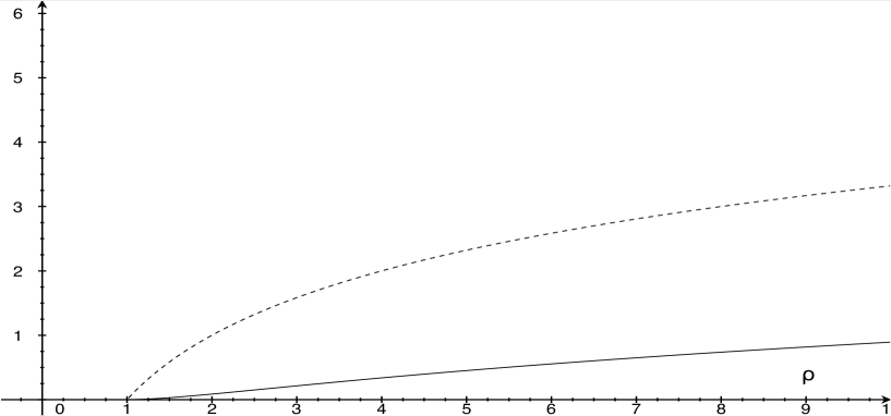
Figure 1: Dashed: $\log{\rho}$, solid: $\left(\frac{{\rho}\ln{\rho}}{{\rho}-1}-1-\ln\frac{{\rho}\ln{\rho}}{{\rho}-1}\right)\frac{1}{\ln 2}$

Moreover, our Theorem 2 can also be useful to quantify how close to the uniform probability distribution is the probability distribution on the leaves of a Tunstall tree. This is an important parameter for the efficient generations of truly random bits from a biased distribution (e.g., [5, 32])

VII Approximating the closest distribution to ${\bf p}$, according to the distance D

In this section we show how Theorems 1 and 2 allow us to design an approximation algorithm for the second problem mentioned in Section III, that is, the problem of constructing a probability distribution $\overline{{\bf q}}=(\overline{q}_{1},\ldots,\overline{q}_{m})$ such that ${\tt D}({\bf p},\overline{{\bf q}})\leq{\tt D}({\bf p},{\bf q}^{*})+0.08608$, where ${\tt D}({\bf p},{\bf q})=2W({\bf p},{\bf q})-H({\bf p})-H({\bf q})$, $W({\bf p},{\bf q})$ is the minimum entropy of a bivariate probability distribution that has ${\bf p}$ and ${\bf q}$ as marginals, and

$${\bf q}^{*}=\mbox{arg}\!\!\min_{{\bf q}\in{\cal P}_{m}}{\tt D}({\bf p},{\bf q}).$$

Our algorithm improves on the result presented in [7], where an approximation algorithm for the same problem with an additive error of $1$ was provided.

Let ${\bf q}$ be the probability distribution constructed in Lemma 5 and let us recall that the first $i_{q}$ components of ${\bf q}$ coincide with the first $i_{q}$ components of ${\bf p}$. In addition, for each $i=i_{q}+1,\dots,m,$ there is a set $I_{i}\subseteq\{i_{q}+1,\dots,n\}$ such that $q_{i}=\sum_{k\in I_{i}}p_{k}$ and the $I_{i}$’s form a partition of $\{i_{q}+1,\dots,n\},$ (i.e., ${\bf q}$ is an aggregation of ${\bf p}$ into $m$ components).

We now build a bivariate probability distribution ${{\bf M}}_{q}=[m_{ij}]$, having ${\bf p}$ and ${\bf q}$ as marginals, as follows:

• in the first $i_{q}$ rows and columns, the matrix ${{\bf M}}_{q}$ has non-zero components only on the diagonal, namely $m_{j\,j}=p_{j}=q_{j}$ and $m_{i\,j}=0$ for any $i,j\leq i_{q}$ such that $i\neq j$;

• for each row $i=i_{q}+1,\dots,m$ the only non-zero elements are the ones in the columns corresponding to elements of $I_{i}$ and precisely, for each $j\in I_{i}$ we set $m_{i\,j}=p_{j}.$

It is not hard to see that ${\bf M}_{q}$ has ${\bf p}$ and ${\bf q}$ as marginals. Moreover we have that $H({\bf M}_{q})=H({\bf p})$ since by construction the only non-zero components of ${\bf M}_{q}$ coincide with the set of components of ${\bf p}.$ Let ${\cal C}({\bf p},{\bf q})$ be the set of all bivariate probability distribution having ${\bf p}$ and ${\bf q}$ as marginals. Recall that $\alpha=1-({1+\ln(\ln 2)})/{\ln 2}<0.08608$. We have that

$${\tt D}({\bf p},{\bf q}) = \min_{{\bf N}\in{\cal C}({\bf p},{\bf q})}2H({\bf N})-H({\bf p})-H({\bf q})$$ (41)

$$= 2H({\bf M}_{q})-H({\bf p})-H({\bf q})$$ (42)

$$= H({\bf p})-H({\bf q})$$ (43)

$$\leq H({\bf p})-H(R_{m}({\bf p}))+\alpha$$ (44)

$$\leq H({\bf p})-H({\bf q}^{*})+\alpha$$ (45)

$$\leq {\tt D}({\bf p},{\bf q}^{*})+\alpha$$ (46)

where (41) is the definition of ${\tt D}({\bf p},{\bf q})$; (42) follows from (41) since ${\bf M}_{q}\in{\cal C}({\bf p},{\bf q})$, $H({\bf M}_{q})=H({\bf p})$, and for all ${\bf N}\in{\cal C}({\bf p},{\bf q})$ one has $H({\bf N})\geq H({\bf p})$; (43) follows from (42) because of $H({\bf M})=H({\bf p})$; (44) follows from Lemma 5; (45) follows from (44), the known fact that ${\bf q}^{*}$ is an aggregation of ${\bf p}$ (see Theorem 8 of [41]) and Lemmas 1 and 2. Finally, the general inequality $H({\bf a})-H({\bf b})\leq{\tt D}({\bf a},{\bf b})$ can be proved in the following way. Let $X$ and $Y$ be arbitrary random variables distributed according to ${\bf a}$ and ${\bf b}$. Then

$$H({\bf a})-H({\bf b})=H(X|Y)-H(Y|X)\leq H(X|Y)+H(Y|X).$$

Therefore

$$H({\bf a})-H({\bf b})\leq\min\bigl{\{}H(X|Y)+H(Y|X)\bigr{\}}={\tt D}({\bf p},{\bf q}),$$

where the minimization is taken with respect to all joint probability distributions of $X$ and $Y$ such that the random variable $X$ is distributed according to ${\bf a}$ and the random variable $Y$ according to ${\bf b}$.

Let $g(x)=1+2(x-1)+2\sqrt{x^{2}-x}$. The bound in [37] tells that if $p_{1}/p_{n}\leq g(x)$ for some $x\geq 1$ then $H({\bf p})\geq\log n-\ln x.$ By inverting the function $y=g(x)$ we get $g^{-1}(y)=\frac{(y+1)^{2}}{4y}$. Therefore, the bound in [37] can be equivalently stated as follows: If $p_{1}/p_{n}\leq{\rho}$ then

$$H({\bf p})\geq\log n-\ln\frac{({\rho}+1)^{2}}{4{\rho}}.$$ (47)

The following figure compares the subtractive term in the bound (47) and the subtractive term in bound given by our Theorem 2. The interesting regime is for $\rho\geq 1$.

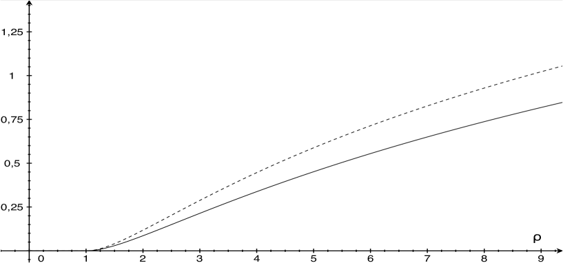
Figure 2: Dashed: $\ln\frac{({\rho}+1)^{2}}{4{\rho}}$, solid: $\left(\frac{{\rho}\ln{\rho}}{{\rho}-1}-1-\ln\frac{{\rho}\ln{\rho}}{{\rho}-1}\right)\frac{1}{\ln 2}.$

References

- [1] J.C. Baez, T. Fritz and T. Leinster, “A characterization of entropy in terms of information loss”, Entropy, vol. 13, n.11, 1945–1957, 2015.
- [2] J. Balatoni and A. Rényi, “Remarks on entropy”, Publ. Math. Inst. Hung. Acad. Sci., vol. 9, 9–-40, 1956.
- [3] F. Cicalese and U. Vaccaro, “Supermodularity and subadditivity properties of the entropy on the majorization lattice”, IEEE Transactions on Information Theory, vol. 48, 933–938, 2002.
- [4] F. Cicalese and U. Vaccaro, “Bounding the average length of optimal source codes via majorization theory”, IEEE Transactions on Information Theory , vol. 50, 633–637, 2004.
- [5] F. Cicalese, L. Gargano, and U. Vaccaro, “A note on approximation of uniform distributions from variable-to-fixed length codes”. IEEE Transactions on Information Theory, vol. 52, No. 8, pp. 3772–3777, 2006.
- [6] F. Cicalese, L. Gargano, and U. Vaccaro,“Information theoretic measures of distances and their econometric applications”, In: Proceedings of 2013 International Symposium in Information Theory (ISIT2013), pp. 409-413, 2013.
- [7] F. Cicalese, L. Gargano, and U. Vaccaro, “Approximating probability distributions with short vectors, via information theoretic distance measures”, in: Proceedings of 2016 IEEE International Symposium on Information Theory (ISIT 2016), pp. 1138-1142, 2016.
- [8] F. Cicalese, L. Gargano, and U. Vaccaro, “ vs. ”, in: Proceedings of 2017 IEEE International Symposium on Information Theory (ISIT 2017), pp. 51–57, Aachen, Germany, 2017.
- [9] R. Cole and H. Karloff,“Fast algorithms for constructing maximum entropy summary trees”, in: Proc. of 41st International Colloquium ICALP 2014, Copenhagen, Denmark, July 8, pp. 332–343, 2014.
- [10] I. Csiszár and P.C. Shields, ‘Information Theory and Statistics: A Tutorial”, Foundations and Trends in Communications and Information Theory: Vol. 1: No. 4, pp. 417-528, 2004.
- [11] R.C. de Amorim and C. Hennig, “Recovering the number of clusters in data sets with noise features using feature rescaling factors”, Information Sciences, vol. 324, pp. 126–-145, 2015.
- [12] A.G. Dimitrov and J.P. Miller, “Neural coding and decoding: communication channels and quantization”, Network: Computation in Neural Systems, Vol. 12, pp. 441–472, 2001.
- [13] A.G. Dimitrov, J.P. Miller, T. Gedeon, Z. Aldworth, and A.E. Parker, “Analysis of neural coding through quantization with an information-based distortion measure”, Network: Computation In Neural Systems, Vol. 14 , pp. 151–176, 2003.
- [14] Z. Dvir, D. Gutfreund, G. Rothblum, and S. Vadhan, “On approximating the entropy of polynomial mappings”. In: Proceedings of the 2nd Innovations in Computer Science Conference, pp. 460–475, 2011.
- [15] L. Faivishevsky and J. Goldberger, “Nonparametric information theoretic clustering algorithm”, in: Proceedings of the 27th International Conference on Machine Learning (ICML-10), pp. 351–358, 2010.
- [16] G. Gan, C. Ma, and J. Wu, Data Clustering: Theory, Algorithms, and Applications, ASA-SIAM Series on Statistics and Applied Probability, SIAM, Philadelphia, ASA, Alexandria, VA, 2007.
- [17] M. R. Garey and D. S. Johnson, Computers and Intractability: A Guide to the Theory of NP-Completeness, W. H. Freeman, 1979.
- [18] B.C. Geiger and R.A. Amjad, “Hard clusters maximize mutual information”, arXiv:1608.04872 [cs.IT]
- [19] S.W. Ho and R.W. Yeung, “The interplay between entropy and variational distance”, IEEE Trans. Inf.. Theory, 56, pp. 5906–5929, 2010.
- [20] S. W. Ho and S. Verdù, “On the interplay between conditional entropy and error probability”, IEEE Trans. Inf. Theory, 56, pp. 5930–5942, 2010.
- [21] F. Jelinek and K.S. Schneider, “On variable-length-to-block coding”, IEEE Transactions on Information Theory, vol. 18, no. 6, pp. 765–774, November 1972.
- [22] A. Kartowsky and Ido Tal, “Greedy-merge degrading has optimal power-law”, in: Proceedings of 2017 IEEE International Symposium on Information Theory (ISIT 2017), pp. 1618–1622, Aachen, Germany, 2017.
- [23] M. Kearns, Y. Mansour, and A. Y. Ng, “An information-theoretic analysis of hard and soft assignment methods for clustering.” In: Learning in graphical models. Springer Netherlands, pp. 495–520, 1998.
- [24] M. Kovačević, I. Stanojević, and V. Senk, “On the entropy of couplings”, Information and Computation, vol. 242, pp. 369–382, 2015.
- [25] B.M. Kurkoski,and H. Yagi, “Quantization of binary-input discrete memoryless channels”, IEEE Transactions Information Theory, vol. 60, 4544 – 4552, 2014.
- [26] B. Nazer, O. Ordentlich, and Y. Polyanskiy, “Information-distilling quantizers”, in: Proceedings of 2017 IEEE International Symposium on Information Theory (ISIT 2017), pp. 96–100, Aachen, Germany, 2017.
- [27] G.-C. Rota, “Twelve problems in probability no one likes to bring up”, in: Algebraic Combinatorics and Computer Science, H. Crapo et al. (eds.), pp. 57–93, Springer-Verlag, 2001.
- [28] J.P.S. Kung, G.-C. Rota, and C.H. Yan, Combinatorics: The Rota Way, Cambridge University Press, 2009.
- [29] R. Lamarche-Perrin, Y. Demazeau, J.-M. Vincent, “The best-partitions problem: How to build meaningful aggregations”, 2013 IEEE/WIC/ACM Inter. Conf. on Web Intell. and Intelligent Agent Techhology, 309–404, 2013.
- [30] P. Malacaria and J. Heusser, “Information theory and security: Quantitative information flow”, in: Aldini A., Bernardo M., Di Pierro A., Wiklicky H. (eds) Formal Methods for Quantitative Aspects of Programming Languages. SFM 2010. Lecture Notes in Computer Science, vol. 6154. Springer, Berlin, Heidelberg, 2010.
- [31] A.W. Marshall, I. Olkin, B. C. Arnold, Inequalities: Theory of Majorization and Its Applications, Springer, New York, 2009.
- [32] M. Mitzenmacher and E. Upfal, Probability and Computing: Randomized Algorithms and Probabilistic Analysis, Cambridge University Press, 2005.
- [33] D. Muresan and M. Effros, “Quantization as histogram segmentation: Optimal scalar quantizer design in network systems”, IEEE Transactions on Information Theory, vol. 54, 344–366, 2008.
- [34] M.A. Nielsen and G. Vidal, “Majorization and the interconversion of bipartite states”, Quantum Information and Computation, vol. 1, no. 1, 76–93, 2001.
- [35] I. Sason, “Entropy bounds for discrete random variables via maximal coupling,” IEEE Trans. on Information Theory, Vol. 59, no. 11, 7118–7131, 2013.
- [36] C. Shannon, “The lattice theory of information”, Transactions of the IRE Professional Group on Information Theory, Vol. 1, pp. 105–107, 1953.
- [37] S. Simic, “Jensen’s inequality and new entropy bounds.” Appl. Math. Letters, 22, 1262–1265, 2009.
- [38] N. Slonim and N. Tishby, “Agglomerative information bottleneck”, in: Advances in Neural Information Processing Systems 12 (NIPS 1999), pp. 617–623. Denver, CO, USA, 1999.
- [39] D.J. Strouse and D.J. Schwab, “The Deterministic information bottleneck”, Neural Computation, vol. 29, no. 6, pp. 1611–1630, 2017.
- [40] N. Tishby, F. Pereira, and W. Bialek, “The Information bottleneck method”, in: The 37th annual Allerton Conference on Communication, Control, and Computing, pp. 368–-377, Monticello, IL., USA, 1999.
- [41] M. Vidyasagar, “A metric between probability distributions on finite sets of different cardinalities and applications to order reduction”, IEEE Transactions on Automatic Control, vol. 57, 2464–2477, 2012.
- [42] I. Wegener, Complexity Theory, Springer-Verlag, 2005.