A discrete harmonic function bounded on a large portion of $\mathbb{Z}^{2}$ is constant

Abstract.

An improvement of the Liouville theorem for discrete harmonic functions on $\mathbb{Z}^{2}$ is obtained. More precisely, we prove that there exists a positive constant $\varepsilon$ such that if $u$ is discrete harmonic on $\mathbb{Z}^{2}$ and for each sufficiently large square $Q$ centered at the origin $|u|\leq 1$ on a $(1-\varepsilon)$ portion of $Q$ then $u$ is constant.

1. Introduction

Let $u$ be a discrete harmonic function on the lattice $\mathbb{Z}^{2}$, i.e., a function satisfying the mean value property: the value of $u$ at any point of $\mathbb{Z}^{2}$ is equal to the average of the four values at the adjacent points.

The Liouville theorem states that if $u$ is bounded on $\mathbb{Z}^{2}$, say $|u|\leq 1$ everywhere, then $u\equiv const$. This statement is classical [2],[6, Theorem 5] and well known.

In the present paper we obtain a somewhat unexpected improvement of the Liouville theorem. We show that if $|u|$ is bounded on $(1-\varepsilon)$ portion of $\mathbb{Z}^{2}$, where $\varepsilon>0$ is a sufficiently small numerical constant, then $u$ is a constant function. The precise statement is given below.

1.1. Main result.

We partition the plane $\mathbb{R}^{2}$ into unit squares (cells) so that the centers of squares have integer coordinates and identify the cells with the elements of $\mathbb{Z}^{2}$.

Given a positive integer $N$, we denote by $Q_{N}$ the square on $\mathbb{Z}^{2}$ with center at the origin and of size $(2N+1)\times(2N+1)$:

$$Q_{N}:=\{(n,m):|n|,|m|\leq N\}.$$

The translation of this square by a vector $x$ with integer coordinates is denoted by $Q_{N}(x)$. For a set $S\subset\mathbb{Z}^{2}$, we denote by $|S|$ the number of elements in $S$.

Let $\varepsilon\in(0,1)$ be a positive number. We say that $|u|$ is bounded by $1$ on $(1-\varepsilon)$ portion of the lattice $\mathbb{Z}^{2}$ if for some $N_{0}>0$

$$|Q_{N}\cap\{|u|\leq 1\}|\geq(1-\varepsilon)|Q_{N}|$$

for all $N\geq N_{0}$.

Theorem 1.1.

There exists $\varepsilon>0$ such that if $u$ is a harmonic function on $\mathbb{Z}^{2}$ and $|u|$ is bounded by $1$ on $(1-\varepsilon)$ portion of $\mathbb{Z}^{2}$, then $u$ is constant.

Remark 1.2.

There is no continuous analog of Theorem 1.1 for harmonic functions in $\mathbb{R}^{2}$. For instance, let $\Pi$ denote the semi-strip $\Pi=\bigl{\{}z\colon\text{Re}(z)>0,\ |\text{Im}(z)|<\pi\bigr{\}}$, and let $L=\partial\Pi$ be oriented so that $\Pi$ is on the right-hand side of $L$. Then the integral

$$E(z)=\frac{1}{2\pi{\rm i}}\int_{L}\frac{e^{e^{\zeta}}}{\zeta-z}\,\text{d}\zeta\,,\qquad z\in\mathbb{C}\setminus\Pi,$$

has an analytic continuation on $\mathbb{C}$, which is bounded outside $\Pi$ (see, for instance, [8, Ch 3, Problems 158-160]). Obviously, the harmonic function $H(z)=\text{Re}E(z)$ is also bounded outside $\Pi$.

Furthermore, given an arbitrarily narrow curvilinear semi-strip $\Pi$, symmetric with respect to the real axis and such that the intersection of $\Pi$ with any vertical line consists of an open interval, replacing the function $e^{\zeta}$ by another analytic function, one can modify this construction to get an entire (and then, harmonic) function bounded outside $\Pi$. See, for instance the discussion in [2].

Remark 1.3.

The following simple example shows that the statement of Theorem 1.1 cannot be extended to higher dimensions. First, we consider the function $u_{0}:\mathbb{Z}^{2}\to\mathbb{R}$ defined by $u_{0}(x,y)=0$ when $x\neq y$ and $u_{0}(x,x)=(-1)^{x}$. This function is not harmonic but is an eigenfunction of the discrete Laplace operator,

$$\Delta u_{0}(x,y)=u_{0}(x+1,y)+u_{0}(x,y+1)+u_{0}(x-1,y)+u_{0}(x,y-1)-4u_{0}(x,y)=-4u_{0}(x,y).$$

Then we define a function on $\mathbb{Z}^{3}$ by

$$u(x,y,z)=c^{z}u_{0}(x,y),\quad{\text{where}}\ \ c+c^{-1}=6,$$

and check that $u$ is a non-zero harmonic function on $\mathbb{Z}^{3}$ that vanishes everywhere except for the hyperplane $\{(x,y,z):x=y\}$.

1.2. Toy question and two examples

A simpler uniqueness question can be asked in connection to Theorem 1.1. Let a discrete harmonic function $u$ be equal to zero on $(1-\varepsilon)$ portion of $\mathbb{Z}^{2}$. Does $u$ have to be zero identically?

Theorem 1.1 implies the affirmative answer to that question if $\varepsilon>0$ is sufficiently small. On the other hand the statement is wrong for $\varepsilon=1/2$. One can construct a non-zero discrete harmonic function $u$ on $\mathbb{Z}^{2}$, which is equal to zero on half of $\mathbb{Z}^{2}$. Namely, $u$ may have zero values on a half-plane $\{(x,y)\in\mathbb{Z}^{2}:x-y\geq 0\}$ without being zero everywhere. It is not difficult to see that on each next diagonal we can choose one value and then the rest of the values are determined uniquely, the details of such construction are given in Section 3.3.

Going back to the assumption of Theorem 1.1, we note that there is a discrete harmonic function, which is bounded on $3/4$ of $\mathbb{Z}^{2}$. The following simple example was drawn to authors’ attention by Dmitry Chelkak. Let

$$u(n,m)=\sin(\pi n/2)e^{bm},$$

where $b$ is the positive solution of $e^{b}+e^{-b}=4$. It is easy to check that $u$ is a discrete harmonic function and $|u|$ is bounded by $1$ on $(2\mathbb{Z}\times\mathbb{Z})\cup(\mathbb{Z}\times\mathbb{Z}_{-})$.

We don’t know the precise value of $\varepsilon$ for either the uniqueness question or the boundedness question. One may also ask if those constants are equal.

1.3. Two theorems

The proof of Theorem 1.1 is based on two statements, which compete with each other.

Theorem (A).

For all sufficiently small $\varepsilon>0$, there exist $a=a(\varepsilon)>0$ and $N_{0}=N_{0}(\varepsilon)$ such that if

$$|Q_{N}\cap\{|u|\leq 1\}|\geq(1-\varepsilon)|Q_{N}|,\quad N>N_{0}(\varepsilon),$$

then

$$\max\limits_{Q_{[N/2]}}|u|\leq e^{aN}.$$

Moreover, $a(\varepsilon)\to 0$ as $\varepsilon\to 0$.

Theorem (B).

There exists $b>0$ such that the following holds. If $\varepsilon>0$ is sufficiently small, $N$ is sufficiently large, $\max\limits_{Q_{[\sqrt{N}]}}|u|\geq 2$ and

$$|Q_{K}\cap\{|u|\leq 1\}|\geq(1-\varepsilon)|Q_{K}|$$

for every $K\in[\sqrt{N},N]$, then

$$\max\limits_{Q_{[N/2]}}|u|\geq e^{bN}.$$

1.4. Theorem 1.1 follows from Theorems (A) and (B)

Assume that $|u|$ is bounded by $1$ on $(1-\varepsilon)$ portion of $\mathbb{Z}^{2}$ and $\varepsilon$ is small enough so that the value of $a$ from Theorem (A) is strictly smaller than the value of $b$ from Theorem (B). If $u$ is not constant, then by the Liouville theorem $\max\limits_{Q_{[\sqrt{N}]}}|u|\geq 2$ for some large $N$. Then the conclusion of Theorem (A) contradicts the conclusion of Theorem (B).

Remark 1.4.

As we have mentioned above, there is no continuous version of Theorem (A), i.e., Theorem (A) is essentially of discrete nature. On the other hand, Theorem (B) has continuous analogs, which are related to a version of the Hadamard three circle theorem for harmonic functions. In fact, a stronger version of Theorem (B) holds for continuous harmonic functions. If $f$ is a non-constant harmonic function on $\mathbb{R}^{2}$, then, informally speaking, the larger the set $\{|f|<1\}$ is, the faster $\max_{|z|=R}|f(z)|$ grows as $R\to\infty$.

It is worth mentioning that we don’t know whether the statement of Theorem 1.1 still holds under the weaker assumption that

$$|Q_{N}\cap\{|u|<1\}|\leq(1-\varepsilon)|Q_{N}|\quad{\text{ for\ infinitely\ many}}\ N.$$

Another open question is whether Theorem 1.1 remains true if one replaces the boundedness by positivity of $u$ on a large portion of $\mathbb{Z}^{2}$ (for $\varepsilon=0$ the result is true and classical [2]).

2. Lower bound

This section is devoted to the proof of Theorem (B).

2.1. Discrete three circle (square) theorem

We will use a discrete version of the Hadamard three circle theorem. Let $u$ be a discrete harmonic function on $Q_{N}$. Given a square $Q_{K}$, we say that $u$ is bounded by $1$ on a half of $Q_{K}$ if

$$|Q_{K}\cap\{|u|\leq 1\}|\geq\frac{1}{2}|Q_{K}|.$$

Theorem 2.1.

If $|u|\leq 1$ on a half of $Q_{[N/4]}$ and $|u|\leq M$ on $Q_{N}$, then

$$\max_{Q_{[N/2]}}|u|\leq CM^{\alpha}+Ce^{-cN}M,$$

where $\alpha\in(0,1)$ and $c,C>0$ are numerical constants.

This is a generalization of the discrete three circle theorem proved in [4], where the estimate $|u|\leq 1$ was assumed on the whole square $Q_{[N/4]}$. The continuous analog of Theorem 2.1 is known, a more general statement can be found in [7]. Comparing the discrete theorem with the continuous one, we see that an error term $Ce^{-cN}M$ appears at the RHS. This term has a discrete nature, cannot be removed and makes the three circle theorem in the discrete case weaker than in the continuous case.

The proof of Theorem 2.1 can be obtained by a modification of the proof given in [4]. A simpler approach is outlined in the Appendix for the convenience of the reader.

2.2. Proof of Theorem (B)

We assume that $N$ is sufficiently large and $\varepsilon$ is sufficiently small. More precisely, if $\alpha$ is as in Theorem 2.1, we first choose a large constant $A$ such that $((1+\alpha)/2)^{A}<2^{-5}$ and then take $\varepsilon<\frac{1}{100A^{2}}$. The choice of the parameters will be justified later.

For each integer $K$, $1\leq K\leq N$, denote by $M(K)$ the maximum of $u$ over $Q_{K}$. The following proposition is the main step in the proof of Theorem (B).

Proposition 2.2.

In assumptions of Theorem (B), there exist $C_{1},c_{1}>0$ such that if $M(K)>C_{1}$ and $K\in[\sqrt{N},N/4]$, then

(1) $$M(2K)\geq\min(M^{32}(K),M(K)e^{c_{1}K}).$$

The constant $32=2^{5}$ depends on our choice of the parameters, it can be replaced by any other constant provided that $\varepsilon$ is sufficiently small.

Proof.

First, by the assumption,

$$|Q_{4K}\cap\{|u|>1\}|\leq\varepsilon|Q_{4K}|.$$

Let $L=[K/A]$. Then, the inequality above and our choice of $\varepsilon$ imply that

(2) $$|Q_{[L/2]}(x)\cap\{|u|\leq 1\}|\geq\frac{1}{2}|Q_{[L/2]}(x)|,$$

for any $x\in Q_{2K}$.

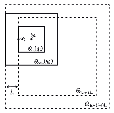
Figure 1.

For $i=0,1,...,A$, denote $M(K+iL)$ by $M_{i}$ and fix $x_{i}\in Q_{K+iL}$ such that $|u(x_{i})|=M_{i}$. Further, we choose $y_{i}$ such that $x_{i}\in Q_{L}(y_{i})\subset Q_{K+iL}$, see Figure 1. By (2) we can apply Theorem 2.1 to the square $Q_{L}(y_{i})$. This gives

$$\max\limits_{Q_{L}(y_{i})}|u|\leq C\max\limits_{Q_{2L}(y_{i})}|u|^{\alpha}+Ce^{-cK/A}\max\limits_{Q_{2L}(y_{i})}|u|.$$

Therefore, we have

$$M_{i}\leq CM^{\alpha}_{i+1}+Ce^{-cK/A}M_{i+1}.$$

Hence, for each $i=0,1,...,A-1$, at least one of the following inequalities holds:

$$(i)\quad M_{i}\leq 2Ce^{-cK/A}M_{i+1},\quad\quad(ii)\quad M_{i}\leq 2CM^{\alpha}_{i+1}.$$

We note that if (i) holds for at least one $i\in[0,A-1]$, then

$$M(2K)\geq M(K)e^{c_{1}K}$$

with sufficiently small $c_{1}$, depending on $c,A,C$ (since $N$ and therefore $K$ is large enough). This finishes the proof of the inequality (1) when (i) holds for at least one $i\in[0,A-1]$.

Assume that (ii) holds for each $i\in[0,A-1]$. Now, we use the assumption that $M(K)>C_{1}$ for some sufficiently large constant $C_{1}$. Denote $\alpha_{1}=\frac{\alpha+1}{2}$. Note that $\alpha_{1}>\alpha$ and

$$M_{i}\leq 2CM^{\alpha}_{i+1}\leq M^{\alpha_{1}}_{i+1},\quad{\text{for}}\quad i=0,...,A-1$$

provided that $C_{1}$ is sufficiently large. Therefore $M_{0}\leq M_{A}^{\alpha_{1}^{A}}$. Hence, by our choice of $A$, $\alpha_{1}^{A}<2^{-5}$, and we get

$$M(K)<\sqrt[32]{M(2K)}.$$

It completes the proof of the proposition. ∎

We continue to prove Theorem (B). We claim that the assumption $M(K)>C_{1}$ in Proposition 2.2 is fulfilled for $K=[N^{3/4}]$ when $N$ is sufficiently large (and then for all larger $K$). Indeed, $M([\sqrt{N}])\geq 2$ and there is at least one cell in $Q_{[\sqrt{N}]}$ where the function is $\leq 1$. Hence there are neighbors $p,p^{\prime}$ in $Q_{[\sqrt{N}]}$ with

$$|u(p)-u(p^{\prime})|\geq\frac{1}{4[\sqrt{N}]}.$$

The discrete gradient estimate for harmonic functions, see [6, Theorem 14] or (15) in Appendix, claims that if $q$ and $q^{\prime}$ are adjacent cells in $Q_{R}$, then

$$|u(q)-u(q^{\prime})|\leq C\max_{Q_{2R}}|u|/R.$$

Hence we have

$$M([N^{3/4}])\geq c_{2}|u(p)-u(p^{\prime})|N^{3/4}\geq c_{3}N^{1/4}\geq C_{1}$$

for $N$ large enough.

Finally we are ready to finish the proof of Theorem (B). Let

$$K_{0}=[N^{3/4}]+1,K_{1}=2K_{0},\dots,K_{l}=2^{l}K_{0},$$

where $K_{l}$ is the largest number in this sequence smaller than $N/2$. Note that $2^{l+3}\geq N^{1/4}$ and hence $32^{l}>N$ when $N$ is large enough. For each $i\in[1,l]$, by Proposition 2.2, we have

(3) $$M(K_{i})\geq\min((M(K_{i-1}))^{32},e^{c_{1}K_{i-1}}M(K_{i-1})).$$

First, we consider the case when for at least one $i\in[1,l]$

(4) $$M(K_{i})\geq e^{c_{1}K_{i-1}}M(K_{i-1}).$$

Then $M(K_{i})\geq e^{c_{1}K_{i-1}}.$ In this case, applying Proposition 2.2 for $i+1$ in place of $i$, we get

$$M(K_{i+1})\geq\min(e^{32c_{1}K_{i-1}},e^{c_{1}K_{i}})=e^{c_{1}K_{i}}.$$

Repeating the argument several times, we obtain

$$\max_{Q_{[N/2]}}|u|\geq M(K_{l})\geq e^{c_{1}K_{l-1}}\geq e^{c_{1}N/8}.$$

So the proof of Theorem (B) is finished if (4) holds for at least one $i\in[1,l]$.

Assume that it does not happen. Then by (3)

$$M(K_{i})\geq(M(K_{i-1}))^{32},\quad i=1,\dots,l.$$

This implies

$$\max_{Q_{[N/2]}}|u|\geq M(K_{l})\geq(M(K_{0}))^{32^{l}}\geq 2^{32^{l}}\geq 2^{N}.$$

The proof of Theorem (B) is completed.

3. Upper bound

3.1. Remez inequality.

The Remez inequality compares $L^{\infty}$ norms of a polynomial on different subsets of real line, we formulate the inequality in a simplified form. The sharp version is proven in the original work [9], see also [1].

Lemma 3.1 (Remez inequality).

Let $p$ be a polynomial of one variable of degree $d$. Suppose also that $I$ is a closed interval on the real line and $E$ is a measurable subset of $I$ with positive measure $|E|$. Then

$$\max_{I}|p|\leq\left(\frac{4|I|}{|E|}\right)^{d}\sup_{E}|p|.$$

We will need a discrete version of the Remez inequality.

Corollary 3.2.

Suppose that a polynomial $p$ of degree less than or equal to $d$ is bounded by $M$ at $d+l$ integer points on a closed interval $I$, then

$$\max_{I}|p|\leq\left(\frac{4|I|}{l}\right)^{d}M.$$

Proof of the corollary..

We may assume that $p$ is not a constant function and therefore $p^{\prime}$ is a non-zero polynomial of degree $\leq d-1$. Let

$$x_{1}<x_{2}<\ldots<x_{d+l}$$

be $d+l$ integer points on $I$ where $|p(x_{j})|\leq M$. If $p^{\prime}$ has no roots on $(x_{i},x_{i+1})$, then $|p|\leq M$ on $[x_{i},x_{i+1}]$. Since $p^{\prime}$ has at most $d-1$ roots, there are at least $l$ intervals $(x_{j},x_{j+1})$ without roots of $p^{\prime}$. At the end points of such intervals $p$ is bounded by $M$ and therefore $p$ is bounded by $M$ on at least $l$ disjoint intervals of length at least one. So the set $\{|p|\leq M\}$ has length at least $l$ and we can apply the Remez inequality in Lemma 3.1.

∎

3.2. Some notation and a reformulation of Theorem (A)

In this section we change our notation and introduce new coordinates which are better adjusted to our argument for the upper bound.

We define $s=(n+m)/2$ and $k=(n-m)/2$, such that $s,k\in\frac{1}{2}\mathbb{Z}$, and we always have $s+k\in\mathbb{Z}$. We denote the set of all such pairs $(s,k)$ by

$$\mathbb{Z}^{2}=\left\{(s,k)\in\frac{1}{2}\mathbb{Z}\times\frac{1}{2}\mathbb{Z}\,:\,s+k\in\mathbb{Z}\right\}.$$

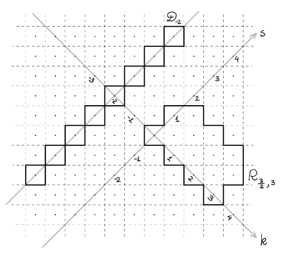
Figure 2.

$\mathbb{Z}^{2}$, the rectangle $R_{3/2,2}$, and the line $D_{-2}$

For $l\in\frac{1}{2}\mathbb{Z}$, denote by $D_{l}$ the set

$$D_{l}=\{(s,k)\in\mathbb{Z}^{2}:k=l\}.$$

We define a rectangle as a subset of $\mathbb{Z}^{2}=\{(s,k)\}$ of the form

$$R=\{a_{1}\leq s\leq a_{2},\,\,b_{1}\leq k\leq b_{2}\}$$

We denote it by $R_{I,J}$, where $I=[a_{1},a_{2}]$ and $J=[b_{1},b_{2}]$ and write $R_{a,b}$ for $I=[0,a]$ and $J=[0,b]$, see Figure 2.

From now on we use new coordinates $(s,k)$. Given a function $u$ on $\mathbb{Z}^{2}$ we identify it with the function $U$ on $\mathbb{Z}^{2}$ defined by

$$U(s,k)=u(s+k,s-k).$$

If $u$ is harmonic on $\mathbb{Z}^{2}$ then $U$ satisfies

(5) $$4U\left(s+\tfrac{1}{2},k+\tfrac{1}{2}\right)=U(s,k)+U(s+1,k)+U(s,k+1)+U(s+1,k+1).$$

We reformulate Theorem (A) using these new notation and we do not use other coordinates till the end of the proof of Theorem (A). We want to prove the following:

Theorem (A^′).

Suppose that function $U$ is defined on $\mathcal{Q}_{N}=R_{[-N,N],[-N,N]}$ and satisfies (5) for all $(s,k)\in\mathbb{Z}^{2}$ such that $-N\leq s\leq N-1,-N\leq k\leq N-1$. Assume further that $|U|\leq 1$ on $(1-\varepsilon)$ portion of $\mathcal{Q}_{N}$ and $\varepsilon>0$ is small enough. Then

$$|U(s,k)|\leq e^{a_{1}(\varepsilon)N},\quad(s,k)\in\mathcal{Q}_{N/2},$$

provided that $N$ is large enough. Moreover $a_{1}(\varepsilon)\to 0$ as $\varepsilon\to 0$.

Theorem (A) follows from Theorem (A^′). Note that to deduce Theorem (A) we apply Theorem (A^′) with a different (but comparable) value of $N$ . We cover the initial square $Q_{[N/2]}$ by several shifted new (sloped) squares and apply the statement in each of them.

3.3. Two elementary observations

Before we start the proof of Theorem (A^′), we make two useful observations.

Let $I=[a_{1},a_{2}],J=[b_{1},b_{2}]$, where $a_{1}\leq a_{2},\ b_{1}\leq b_{2}$ and $a_{1},a_{2},b_{1},b_{2}\in\tfrac{1}{2}\mathbb{Z}$. We consider the rectangle $R_{I,J}$ and denote by $a(R)$ and $b(R)$ its side lengths $a(R)=a_{2}-a_{1}+1/2$ and $b(R)=b_{2}-b_{1}+1/2$.

Observation 1.

Let $U$ be any function defined on the set

$$S=\{(s,k)\in R_{I,J}:\min\{s-a_{1},k-b_{1}\}\in\{0,1/2\}\}$$

Then $U$ has a unique discrete harmonic extension to $R=R_{I,J}$. This extension satisfies

$$\max_{R}|U|\leq 7^{a(R)+b(R)}\max_{S}|U|.$$

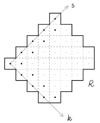
Figure 3.

The square $R$ and its subset $S$ (black points)

Proof.

Without loss of generality we may assume $\max_{S}|U|=1$. We are going to prove that the extension is unique and satisfies

(6) $$|U(s,k)|\leq 7^{s+k-a_{1}-b_{1}}\quad{\text{for\ all}}\ (s,k)\in R.$$

We argue by induction on $k$ and for fixed $k$ by induction on $s$. Recall that $D_{l}=\{(s,k)\in\mathbb{Z}^{2},k=l\}$ and let $T_{l}=D_{l}\cap R$. Clearly on $T_{b_{1}}$ and $T_{b_{1}+1/2}$ the function is already defined and the inequality (6) holds.

Suppose that we have proved that $U$ is uniquely determined and satisfies the estimate on $R_{k}:=\mathop{\cup}_{b_{1}\leq i\leq k}T_{i}$. The value of $U(s,k+1/2)$ is prescribed at the first point of $T_{k+1/2}$, where $s=a_{1}$ or $s=a_{1}+1/2$ (depending on the value of $k$), and the inequality (6) holds. Furthermore, the extension has to satisfy the mean value property (5) for the cells $(s,k)$ on $T_{k}$ with $a_{1}<s<a_{2}$,

$$U(s+\tfrac{1}{2},k+\tfrac{1}{2})=4U(s,k)-U(s+\tfrac{1}{2},k-\tfrac{1}{2})-U(s-\tfrac{1}{2},k-\tfrac{1}{2})-U(s-\tfrac{1}{2},k+\tfrac{1}{2}).$$

Thus by induction on $s$ the values on $T_{k+1/2}$ are uniquely determined.

Furthermore, since estimate (6) holds on $T_{k}$ and $T_{k-1/2}$, we have

$$|U(s+\tfrac{1}{2},k+\tfrac{1}{2})|\leq 6\cdot 7^{s+k-a_{1}-b_{1}}+|U(s-\tfrac{1}{2},k+\tfrac{1}{2})|,\quad a_{1}<s<a_{2}.$$

So if (6) holds at $(s-\tfrac{1}{2},k+\tfrac{1}{2})$, then it also holds at $(s+\tfrac{1}{2},k+\tfrac{1}{2})$. The induction argument finishes the proof. ∎

Observation 2.

Assume that a discrete harmonic function $U$ on $R=R_{I,J}$ satisfies

$$U(s,b_{1})=U(s,b_{1}+\tfrac{1}{2})=0,\quad a_{1}\leq s\leq a_{2}.$$

Then for any $k\in[b_{1}+1,b_{2}]\cap\frac{1}{2}\mathbb{Z}$ there is a polynomial $p_{k}$ of degree not greater than $2(k-b_{1})-2$ such that

(7) $$U(s,k)=(-1)^{s+k}p_{k}(s),\quad a_{1}\leq s\leq a_{2}.$$

Proof.

Define the functions $p_{k}(s)$ by (7). We show by induction on $k$ that $p_{k}$ coincides with some polynomial of degree $\leq 2(k-b_{1})-2$. The basis of induction follows from the fact that $U(s,k)=0$ for $k=b_{1},b_{1}+1/2$ (by a polynomial of a negative degree we mean identically zero function). We prove the statement for $k$ assuming that it holds for $k-1/2$ and $k-1$. By the mean value property (5) for $U$, we have

$$p_{k}(s+1)-p_{k}(s)=-4p_{k-1/2}(s+\tfrac{1}{2})+p_{k-1}(s+1)-p_{k-1}(s),\quad a_{1}\leq s\leq a_{2}-1.$$

Then, by the induction assumption, $p_{k}(s+1)-p_{k}(s)$ coincides on $a_{1}\leq s\leq a_{2}-1$ with a polynomial of degree $\leq 2(k-b_{1})-3$. Thus $p_{k}(s)$ coincides on $a_{1}\leq s\leq a_{2}$ with some polynomial of degree not greater than $2(k-b_{1})-2$. ∎

The next corollary is an application of the Remez inequality.

Corollary 3.3.

Assume that the rectangle $R=R_{I,J}$ satisfies $a(R)\geq 10b(R)$. Assume also that a discrete harmonic function $U$ on $R$ satisfies

$$U(s,b_{1})=U(s,b_{1}+\tfrac{1}{2})=0,\quad a_{1}\leq s\leq a_{2},$$

and $|U(s,b_{2})|\leq M$ for at least half of the points $(s,b_{2})$ on $T_{b_{2}}=D_{b_{2}}\cap R$. Then the following inequality holds:

$$|U(s,b_{2})|\leq MC^{b(R)},\quad a_{1}\leq s\leq a_{2}.$$

Proof.

Indeed, by the observation $(-1)^{s+b_{2}}U(s,b_{2})$ coincides with a polynomial $p(s)$ of degree not greater than $2b(R)-3$. But the number of cells in $D_{b_{2}}\cap R$ is at least $a(R)-1\geq 5(2b(R)-3)$ and $|p|\leq M$ on at least half of those cells. Applying the discrete version of the Remez inequality for $p$ we obtain a bound for $|p|$ on the interval $[a_{1},a_{2}]$. It gives the required bound for $|u|$ on $T_{b_{2}}$. ∎

3.4. Auxiliary Lemma

We will use the following lemma several times in the proof of Theorem (A).

Lemma 3.4.

Let $U$ be a discrete harmonic function on a rectangle $R=R_{I,J}$ with $a(R)\geq 10b(R).$ If

$$|U(s,b_{1})|,|U(s,b_{1}+\tfrac{1}{2})|\leq M,\quad a_{1}\leq s\leq a_{2},$$

and $|U|\leq M$ on at least half of the cells of $T_{b_{2}}=D_{b_{2}}\cap R$, then

$$|U(s,k)|\leq MC_{1}^{a(R)},\quad{\text{ for\ all}}\quad(s,k)\in R.$$

Proof.

We divide the proof into several steps.

Step 1. First, we prove the estimate $|U|\leq MC_{2}^{a(R)}$ on $T_{b_{2}}$. It is enough to consider the case when $U$ is zero on the set $S_{0}=\{(s,k)\in R,k=b_{1},b_{1}+1/2\}$. Indeed, we can apply Observation 1 to find a discrete harmonic function $U_{1}$ in $R$, which coincides with $U$ on the set $S_{0}$ and for example is zero at $(s,k)\in R$ such that $s\in\{a_{1},a_{1}+1/2\}$ and $k>b_{1}+1/2$. We see also that $|U_{1}|\leq 7^{a(R)+b(R)}M\leq M7^{2a(R)}$ in $R$. Now, consider the function $U_{2}=U-U_{1}$, which is equal to zero on $S_{0}$ and is less than $(1+7^{2a(R)})M$ on at least half of the cells of $T_{b_{2}}$. Corollary 3.3, applied for $U_{2}$, yields the bound $|U_{2}|\leq C^{b(R)}(1+7^{2a(R)})M$ on $T_{b_{2}}$. Thus $|U|$ is bounded on $T_{b_{2}}$ by $(C^{b(R)}(1+7^{2a(R)})+7^{2a(R)})M\leq MC_{2}^{a(R)}$.

Step 2. Suppose that $U$ is discrete harmonic in $R=R_{I,J}$ with $a(R)\geq 10b(R)$ and that

(8) $$|U(s,b_{1})|,|U(s,b_{1}+1/2)|,|U(s,b_{2})|\leq M_{1}\quad{\text{for\ any}}\quad a_{1}\leq s\leq a_{2}.$$

Then, we prove by induction on $b(R)$, that

(9) $$|U(s,k)|\leq M_{1}9^{b(R)}\quad{\text{for}}\ (s,k)\in\mathbb{Z}^{2},\ a_{1}+b(R)\leq s\leq a_{2}-b(R),\ b_{1}\leq k\leq b_{2}.$$

If $b(R)\leq 3/2$ all the values of $|U|$ are bounded by $M_{1}$. This is the basis of induction. For the induction step assume $b(R)>3/2$.

Define the function $V$ on $R^{-}=\{(s,k)\in\mathbb{Z}^{2}:a_{1}\leq s\leq a_{2}-1,b_{1}+1/2\leq k\leq b_{2}\}$ by

$$V(s,k)=U(s,k)+U(s+1,k).$$

Note that $V$ is discrete harmonic in $R^{-}$ and clearly $|V|\leq 2M_{1}$ on $D_{b_{1}+1/2}\cap R^{-}$ and on $D_{b_{2}}\cap R^{-}$. We claim that $|V|\leq 6M_{1}$ on $D_{b_{1}+1}\cap R^{-}$. By the mean value property (5),

$$V(s,b_{1}+1)=U(s,b_{1}+1)+U(s+1,b_{1}+1)=4U(s+1/2,b_{1}+1/2)-U(s,b_{1})-U(s+1,b_{1}).$$

Since $|U|\leq M_{1}$ on $D_{b_{1}}\cap R$ and on $D_{b_{1}+1/2}\cap R$, the identity above implies $|V|\leq 6M_{1}$ on $D_{b_{1}+1}\cap R^{-}$.

Now, we know that $|V|\leq 6M_{1}$ on three lines: $D_{b_{1}+1/2}\cap R^{-},D_{b_{1}+1}\cap R^{-}$ and $D_{b_{2}}\cap R^{-}$. We are in position to apply the induction assumption for $V$ and $R^{-}$. It gives

$$|V(s,k)|\leq 6M_{1}9^{b(R^{-})},\quad a_{1}+b(R^{-})\leq s\leq a_{2}-1-b(R^{-}),\ b_{1}+1/2\leq k\leq b_{2}.$$

Applying (5) once again, we get

$$4U(s,k)=V(s-1/2,k-1/2)+V(s-1/2,k+1/2).$$

For every $(s,k)\in\mathbb{Z}^{2}$, $a_{1}+b(R)\leq s\leq a_{2}-b(R)$, $b_{1}+1\leq k\leq b_{2}-1/2,$ it yields

$$|U(s,k)|\leq M_{1}9^{b(R)}.$$

While on $D_{b_{1}}\cap R$, $D_{b_{1}+1/2}\cap R$, and $D_{b_{2}}\cap R$ the function $|U|$ is smaller than $M_{1}$ by the initial assumption. The induction step is completed. We therefore have proved (9).

Step 3 Finally, applying Observation 1 to rectangles $R_{[a_{1},a_{1}+b(R)+1/2],J}$ and $R_{[a_{2}-b(R)-1/2,a_{2}],J}$, we obtain

$$|U(s,k)|\leq M_{1}9^{b(R)}7^{b(R)+1}\leq M_{1}C_{3}^{b(R)},{\text{ for\ all}}\quad(s,k)\in R_{I,J}.$$

Now we combine the steps. The first step implies (8) with $M_{1}=MC_{2}^{a(R)}$, then Steps 2 and 3 give $|U(s,k)|\leq M_{1}C_{3}^{b(R)}\leq MC_{2}^{a(R)}C_{3}^{b(R)}\leq MC_{1}^{a(R)}$ for all $(s,k)\in R$. This completes the proof of Lemma 3.4. ∎

3.5. Good rectangles

We make the last preparation for the proof of Theorem (A). Let $\mathcal{Q}=\mathcal{Q}_{N}=R_{[-N,N],[-N,N]}$ as in Section 3.2. We fix a function $U:\mathcal{Q}\rightarrow\mathbb{R}$ which is discrete harmonic and such that $|U|\leq 1$ on $(1-\varepsilon)$ portion of $\mathcal{Q}$.

We consider ”good rectangles” $R_{[a_{1},a_{2}],[b_{1},b_{2}]}=\{(s,k)\in\mathbb{Z}^{2}:a_{1}\leq s\leq a_{2},b_{1}\leq k\leq b_{2}\}$, whose side-lengths $a(R)=a_{2}-a_{1}+1/2$ and $b(R)=b_{2}-b_{1}+1/2$ are comparable, and on which the function $U$ is not large. More precise definition is below.

Definition 3.5.

Let $A=C_{1}^{800}$, where $C_{1}$ is the constant from Lemma 3.4. A rectangle $R\subset\mathcal{Q}$ is called good, if

$$a(R)/10\leq b(R)\leq 10a(R)\quad{\text{and}}\quad\max_{R}|U|\leq A^{a(R)+b(R)}.$$

The following lemma helps to expand good rectangles. It claims that if there is a good rectangle and near this rectangle the portion of cells with $|U|>1$ is small, then one can find a new larger good rectangle that contains the old one. For simplicity we formulate it for rectangles $R_{I,J}$ with $I=[0,a]$ and $J=[0,b]$ but will apply it for general rectangles, the proof is the same up to small changes of notation.

Lemma 3.6.

Assume that $R_{a,b}$ is a good rectangle with $a\geq b\geq 1/2$ and that the number of cells in $R_{a,3b}$ where $|U|>1$ is less than $\frac{1}{10^{5}}|R_{a,b}|$. Then for any $b^{\prime}\in[3b/2,2b]$, the rectangle $R_{a,b^{\prime}}$ is also good.

Proof.

If $b\leq 40$, then $a\leq 400$ because $R_{a,b}$ is good. In this case $|R_{a,4b}|\leq 10^{5}$ and $|U|\leq 1$ everywhere on $R_{a,4b}$.

Assume that $b>40$. For each $k=1,2,\dots,40$ we can choose a number

$$b_{k}\in\frac{1}{2}\mathbb{Z}\cap(b(1+(2k-1)/40),b(1+2k/40))$$

such that at least half of cells $z$ on the line $D_{b_{k}}\cap R_{a,3b}$ satisfy $|U(z)|\leq 1$. Define $b_{0}=b$. Note that

$$b/40\leq b_{k}-b_{k-1}\leq 3b/40\leq 3a/40\leq a/10-1/2$$

and $b_{40}\in(2b,3b)$.

Denote by $M_{k}=\max_{R_{a,b_{k}}}|U|$. It suffices to show that $M_{40}\leq A^{a+\frac{3}{2}b+1}.$ Indeed, it implies that

$$\max_{R_{a,b^{\prime}}}|U|\leq\max_{R_{a,2b}}|U|\leq M_{40}\leq A^{a+\frac{3}{2}b+1}\leq A^{a+b^{\prime}+1},$$

and thus that $R_{a,b^{\prime}}$ is good.

Since $R_{a,b}$ is good, we know that $M_{0}\leq A^{a+b+1}$. We show that

$$M_{k+1}\leq M_{k}C_{1}^{a}\quad{\text{for}}\ k=0,1,2,\dots 40.$$

Consider the rectangle

$$R_{k}=\{(s,t)\in\mathbb{Z}^{2}:0\leq s\leq a,b_{k}-1/2\leq t\leq b_{k+1}\}$$

and note that $b_{k+1}-b_{k}+1/2\leq a/10$. We have $|U|\leq M_{k}$ on $R_{k}\cap D_{b_{k}-1/2}$ and $R_{k}\cap D_{b_{k}}$ and also $|U|\leq 1$ on half of cells of $R_{k}\cap D_{b_{k+1}}$. We therefore can apply Lemma 3.4. We get $|U|\leq M_{k}C_{1}^{a}$ on $R_{k+1}$ and hence

$$M_{k+1}\leq M_{k}C_{1}^{a}.$$

Recalling that $M_{0}\leq A^{a+b+1}$ and using the inequality above consecutively for $k=0,1,...,39$, we get

$$M_{40}\leq A^{a+b+1}C_{1}^{40a}\leq A^{a+\frac{3}{2}b+1},$$

provided that $A\geq C_{1}^{800}$. ∎

Given a square $R=R_{I,J}$ with $I=[a_{1},a_{1}+l]$, $J=[b_{1},b_{1}+l]$ and $a(R)=b(R)=l+1/2$ and an odd integer $n$, we denote by $nR$ the square with the same center and side length $a(nR)=b(nR)=n(l+1/2)$.

Corollary 3.7.

If $R\subset\mathcal{Q}$ is a good square and $9R\subset\mathcal{Q}$, then either

$$|9R\cap\{|U|>1\}|\geq\frac{1}{10^{5}}|R|,$$

or $3R$ is good.

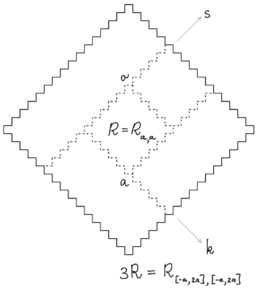
Figure 4.

Proof.

Assume that the number of cells $z$ in $9R$ with $|U(z)|>1$ is less than $\frac{1}{10^{5}}|R|$. Then applying (rotated and shifted versions of) Lemma 3.6 four times, we can expand $R$ and show that $3R$ is good. If we shift the initial square to be $R_{a,a}$ then we obtain the following sequence of good rectangles $R_{a,a},R_{2a,a},R_{2a,2a},R_{[-a,2a],[0,2a]}$ and finally $3R=R_{[-a,2a],[-a,2a]}$. ∎

3.6. Maximal good squares and a covering lemma

For the proof of Theorem (A^′) we will consider good squares that are maximal with respect to inclusion and therefore the portion of cells near these squares with $|U|>1$ is not too small.

Definition 3.8.

We call a good square $R\subset\mathcal{Q}_{N}$ maximal for $\mathcal{Q}_{N}$ if there is no good square $R^{\prime}$ such that $R\subsetneq R^{\prime}\subset\mathcal{Q}_{N}$.

Now, we formulate a proposition to be used in the proof of Theorem (A^′).

Proposition 3.9.

Suppose that

$$|\mathcal{Q}_{K}\cap\{|U|>1\}|\leq 10^{-20}|\mathcal{Q}_{K}|.$$

Then there is a good square $R$ such that

$$\mathcal{Q}_{[K/100]}\subset R\subset\mathcal{Q}_{K}.$$

Proof.

Consider the collection $\mathbb{M}$ of all maximal for $\mathcal{Q}_{[K/10]}$ squares that contain at least one cell in $\mathcal{Q}_{[K/100]}$. Note that the total number of cells in all maximal squares satisfies

(10) $$|\bigcup\limits_{\mathbb{M}}R|\geq\frac{1}{2}|\mathcal{Q}_{[K/100]}|\geq\frac{1}{10^{5}}|\mathcal{Q}_{K}|.$$

This is true because each cell $z\in\mathcal{Q}_{[K/100]}$ with $|U(z)|\leq 1$ is contained in some maximal square and $\{|U|\leq 1\}$ occupies at least a half of $\mathcal{Q}_{[K/100]}$.

We consider two cases:
(1) $a(R_{0})\geq K/50$ for some $R_{0}\in\mathbb{M}$, (2) $a(R)\leq K/50$ for every $R\in\mathbb{M}$.

We show that in the first case the conclusion of Proposition 3.9 holds and that the second case never occurs.

First, suppose that there is $R_{0}\in\mathbb{M}$ with $a(R_{0})\geq K/50.$ Since $R_{0}\subset\mathcal{Q}_{[K/10]}$, we have $9R_{0}\subset\mathcal{Q}_{K}$. Further,

$$|\{|U|>1\}\cap 9R_{0}|\leq|\{|U|>1\}\cap\mathcal{Q}_{K}|\leq 10^{-20}|\mathcal{Q}_{K}|\leq 10^{-7}|R_{0}|.$$

Applying Corollary 3.7 for $R_{0}$ we conclude that $3R_{0}$ is also good. Since $R_{0}$ intersects $\mathcal{Q}_{[K/100]}$ and $a(R_{0})>K/50$, we see that the good square $R=3R_{0}$ contains $\mathcal{Q}_{[K/100]}$ and the proposition is proved in the first case.

For the second case, we have $a(R)\leq K/50$ for each $R\in\mathbb{M}$. Consider any $R\in\mathbb{M}$. Since $R$ intersects $\mathcal{Q}_{[K/100]}$ we see that $3R\subset\mathcal{Q}_{[K/10]}$. Thus, by the maximality of $R$ in $\mathcal{Q}_{[K/10]}$, $3R$ is not good. Then Corollary 3.7 implies

(11) $$|9R\cap\{|U|>1\}|\geq\frac{1}{10^{5}}|R|.$$

We will use the following Vitali-type covering lemma:
Given a finite collection $\mathcal{M}=\{q_{j}\}$ of squares with sides parallel to the coordinate axis, there exists a subcollection $\mathcal{M}^{\prime}=\{q_{j_{k}}\}$ such that $q_{j_{k}}$ are pairwise disjoint and

$$\bigcup_{\mathcal{M}^{\prime}}3q_{j_{k}}\supset\bigcup_{\mathcal{M}}q_{j}.$$

The statement is simple and is proved by selecting the largest possible square on each step such that the chosen subcollection remain disjoint, we refer the reader to [5, Chapter 1]. A similar standard argument for balls in $\mathbb{R}^{n}$ can be found for example in [10].

Let $\mathbb{M}$ be the collection of maximal squares as above. We apply the covering lemma to the collection of squares $9R$ for $R\in\mathbb{M}$. (Note also that $9R\subset\mathcal{Q}_{K}$ for each $R\in\mathbb{M}$.) There exists a subcollection $\mathbb{M}^{\prime}\subset\mathbb{M}$ such that

$$\mathop{\bigcup}\limits_{\mathbb{M^{\prime}}}27R\supset\mathop{\bigcup}\limits_{\mathbb{M}}9R$$

and $9R_{1}$ and $9R_{2}$ are disjoint for any distinct $R_{1},R_{2}\in\mathbb{M^{\prime}}$. Then we get

$$\sum_{\mathbb{M}^{\prime}}|R|\geq\frac{1}{10^{3}}|\mathop{\bigcup}\limits_{\mathbb{M}}R|$$

and, since $\{9R,R\in\mathbb{M}^{\prime}\}$ are disjoint, (11) implies

$$|\{|U|>1\}\cap\mathcal{Q}_{K}|\geq\sum_{R\in\mathbb{M}^{\prime}}|9R\cap\{|U|>1\}|\geq\sum_{R\in\mathbb{M}^{\prime}}\frac{1}{10^{5}}|R|.$$

Thus

$$|\{|U|>1\}\cap\mathcal{Q}_{K}|>\frac{1}{10^{10}}|\mathop{\bigcup}\limits_{\mathbb{M}}R|$$

and by (10)

$$|\{|U|>1\}\cap\mathcal{Q}_{K}|\geq\frac{1}{10^{15}}|\mathcal{Q}_{K}|.$$

This contradicts the assumption of the proposition, hence the second case never occurs. Therefore we can always cover $\mathcal{Q}_{[K/100]}$ by a good rectangle. ∎

3.7. Proof of Theorem (A^′)

By the assumption

$$|\mathcal{Q}_{N}\cap\{|U|\leq 1\}\}|\geq(1-\varepsilon)|\mathcal{Q}_{N}|.$$

Our goal is to show that if $\varepsilon>0$ is sufficiently small and $N$ is sufficiently large, $N\geq N(\varepsilon)$, then

$$\max\limits_{\mathcal{Q}_{N/2}}|U|\leq e^{a_{1}N},$$

where $a_{1}=a_{1}(\varepsilon)\to 0$ as $\varepsilon\to 0$.

Let $K<N/200$ and cover $\mathcal{Q}_{N/2}$ by $\simeq([N/K])^{2}$ squares $\mathcal{Q}_{K}(x_{i})$ such that $\mathcal{Q}_{100K}(x_{i})\subset\mathcal{Q}_{N}$. The number of cells in $\mathcal{Q}_{100K}(x_{i})$ with $|U|>1$ is less than $\varepsilon|\mathcal{Q}_{N}|$. Hence

$$|\mathcal{Q}_{100K}(x_{i})\cap\{|U|>1\}\}|\leq\varepsilon\left(\frac{N}{K}\right)^{2}|\mathcal{Q}_{K}|.$$

If we assume that $K=cN$ and $\varepsilon\leq c^{2}/10^{20}$, then by Proposition 3.9, for each $i$, there is a good square $R_{i}$ such that $\mathcal{Q}_{K}(x_{i})\subset R_{i}\subset\mathcal{Q}_{100K}(x_{i})$. By the definition of a good square we have

$$\max_{R_{i}}|U|\leq A^{200K}=e^{N200c\log A}$$

Thus $|U|\leq e^{N200c\log A}$ in each $\mathcal{Q}_{K}(x_{i})$ and therefore in $\mathcal{Q}_{N/2}$. We had proved the first part of Theorem (A^′).

To prove that $a_{1}(\varepsilon)\to 0$ as $\varepsilon\to 0$, we fix any $a_{1}>0$ and choose $K=K(N,a_{1},\varepsilon)$ so that

$$A^{200K}\leq e^{a_{1}N}\ \textup{ and }\ \varepsilon\left(\frac{N}{K}\right)^{2}\leq 1/10^{20},$$

and we can make such a choice if $\varepsilon$ is sufficiently small.

Appendix

The aim of the appendix is to prove Theorem 2.1. The proof is a modification of the one given in [4]. First, we write down explicit formulas for the discrete Poisson kernel and prove an estimate for its analytic continuation into the complex plane, as it was done in [4]. Then we apply polynomial approximation and the discrete version of the Remez inequality to finish the proof. Note that we return to the standard lattice $\mathbb{Z}^{2}$ and the notation used in the first part of the text.

A.1. The discrete Poisson kernel

For each integer $k\in(0,2N)$ we define $a_{k}$ to be the only positive solution of the equation

$$\cosh a_{k}=2-\cos\frac{k\pi}{2N}.$$

Then

$$f_{k}(n,m)=\sin\left(\frac{\pi kn}{2N}\right)\sinh(a_{k}m)$$

is a discrete harmonic function. Now we fix an integer $n_{1}\in[-N+1,N-1]$ and consider a discrete harmonic function of $(n,m)$

(12) $$F(n,m)=\frac{1}{N}\sum_{k=1}^{2N-1}\sin\left(\pi k\frac{n+N}{2N}\right)\sin\left(\pi k\frac{n_{1}+N}{2N}\right)\frac{\sinh a_{k}(m+N)}{\sinh 2a_{k}N}.$$

Clearly $F(-N,m)=F(N,m)=F(n,-N)=0$. Furthermore, by the orthogonality identities for discretized trigonometric functions, we have $F(n_{1},N)=1$ and $F(n,N)=0$ when $n\neq n_{1},-N<n<N$. Thus $F(n,m)$ is the discrete Poisson kernel for the domain $Q_{N}$ at the boundary point $y=(n_{1},N)$. We denote it by $P(x,y)$, where $x=(n,m)$. Poisson kernel on the three other sides of the square can be computed in a similar way. We define the boundary of $Q_{N}$ by

$$\partial Q_{N}=\{(n_{1},m_{1})\in Q_{N}:\max\{|n_{1}|,|m_{1}|\}=N,\ |n_{1}|\neq|m_{1}|\},$$

it consists of the four sides of the square without the corners, denote the set of these four corners by $K_{N}$. The values of a discrete harmonic function on $Q_{N}\setminus K_{N}$ are defined by its values on $\partial Q_{N}$. More precisely, for any discrete harmonic function $u$ in $Q_{N}$, we have

(13) $$u(x)=\sum_{y\in\partial Q_{N}}P(x,y)u(y),\quad x\in Q_{N}\setminus K_{N}.$$

We need the following statement.

Lemma A.1.

For any $y\in\partial Q_{N}$ and any integer $m\in[-N/2,N/2]$ the function $g(t)=P((tN,m),y)$ has a holomorphic extension on

$$\Omega=\{z:|{\rm{Re}}(z)|\leq 1/2,|{\rm{Im}}(z)|\leq 1/16\}\subset\mathbb{C},$$

this extension satisfies $|g(z)|\leq CN^{-1}$ for all $z\in\Omega$.

Proof.

The holomorphic extension is given by (12). We want to prove the estimate. Let $y=(n_{1},m_{1})$, we consider two cases: $|n_{1}|=N$ and $|m_{1}|=N$. We note that $\cosh a_{k}=2-\cos\frac{k\pi}{2N}$, and we claim that $a_{k}\geq\frac{k}{2N}$. First when $N\leq k\leq 2N$, we have

$$\cosh a_{k}=2-\cos\frac{k\pi}{2N}\geq 2$$

and thus $a_{k}\geq 1\geq\frac{k}{2N}$ because $\cosh 1=(e+e^{-1})/2<2$.

For $0\leq k\leq N$ we use the inequality $\cos x\leq 1-x^{2}/\pi$ when $0\leq x\leq\pi/2$ and we obtain

$$\cosh a_{k}\geq 1+\frac{k^{2}\pi}{4N^{2}}$$

which implies

$$2\sinh^{2}a_{k}/2=\cosh a_{k}-1\geq\frac{k^{2}\pi}{4N^{2}}\geq\frac{k^{2}}{2N^{2}}.$$

We have that $\sinh 0=0$, $(\sinh t)^{\prime}=\cosh t$ and $\cosh t$ is increasing when $t>0$. Then $\sinh t/2\leq t/2\cosh 1\leq t$ for $t\leq 1$. Taking $t=k/(2N)$ we see that $\sinh a_{k}/2\geq t\geq\sinh t/2$ and

$$a_{k}\geq\frac{k}{2N}.$$

Then, for the first case we have,

$$|g(z)| =|P((zN,m),(\pm N,m_{1}))|$$

$$\leq\frac{1}{N}\sum_{k=1}^{2N-1}\left|\frac{\sinh a_{k}N(z+1)}{\sinh 2a_{k}N}\right|$$

$$\leq\frac{1}{N}\sum_{k=1}^{2N-1}\frac{\cosh 3a_{k}N/2}{\sinh 2a_{k}N}\quad\quad(|{\rm{Re}}(z)|\leq 1/2)$$

$$\leq\frac{1}{N}\sum_{k=1}^{2N-1}\frac{1}{\sinh a_{k}N/2}\quad\quad(\sinh 2t\geq\cosh 3t/2\sinh t/2)$$

$$\leq\frac{C}{N}\quad\quad(a_{k}N/2\geq k/4).$$

Similarly, for the case $|m_{1}|=N$, we get

$$|g(z)| =|P((zN,m),(n_{1},\pm N)|$$

$$\leq\frac{1}{N}\sum_{k=1}^{2N-1}\left|\sin\frac{\pi k(z+1)}{2}\right|\frac{\sinh(3a_{k}N/2)}{\sinh 2a_{k}N}$$

$$\leq\frac{1}{N}\sum_{k=1}^{2N-1}\cosh\frac{\pi k}{32}\frac{\sinh(3a_{k}N/2)}{\sinh 2a_{k}N}\quad\quad(|{\rm{Im}}(z)|\leq 1/16)$$

$$\leq\frac{1}{N}\sum_{k=1}^{2N-1}\cosh\frac{a_{k}N}{4}\frac{\sinh(3a_{k}N/2)}{\sinh 2a_{k}N}\quad\quad(\pi k/32\leq k/8\leq a_{k}N/4)$$

$$\leq\frac{1}{N}\sum_{k=1}^{2N-1}\frac{\sinh(7a_{k}N/4)}{\sinh 2a_{k}N}\quad\quad(\sinh(s+t)\geq\cosh s\sinh t,\ s,t>0)$$

$$\leq\frac{1}{N}\sum_{k=1}^{2N-1}\frac{1}{\cosh a_{k}N/4}$$

$$\leq\frac{C}{N}\quad\quad(a_{k}N/4\geq k/8).$$

∎

Corollary A.2.

Suppose that $u$ is a discrete harmonic function on $Q_{N}$ such that $|u|\leq M$ on $Q_{N}$ and that $m_{0}$ satisfies $|m_{0}|<N/2$. Then there exists an analytic function $f=f_{m_{0}}$ defined in a neighborhood of $\Omega=\{z=s+it,|s|\leq 1/2,|t|\leq 1/16\}$ such that $u(n,m_{0})=f(n/N)$ and $|f|\leq C_{0}M$ in $\Omega$.

The corollary follows immediately from Lemma A.1 and the Poisson representation formula (13). We will use this quantitative analyticity of $f$ for the following estimate. Let $P_{d}$ be the Taylor polynomial of $f$ of degree $d$ centered at the origin. Then the standard Cauchy estimate implies

(14) $$|f(z)-P_{d}(z)|\leq\max_{\Omega}|f|(L|z|)^{d+1},\quad|z|<1/L,$$

for some $L=L(\Omega)$.

We remark also that the corollary above, combined with the Cauchy estimates for derivatives of analytic functions, implies that if $q,q^{\prime}\in Q_{N/3}$ are two neighboring cells then

(15) $$|u(q)-u(q^{\prime})|\leq CN^{-1}\max_{Q_{N}}|u|$$

for any discrete harmonic function $u$ in $Q_{N}$. This in turn implies the gradient estimate that we used in the proof of Theorem (B).

Proof of Theorem 2.1

To prove Theorem 2.1, it is enough to prove the following statement for some $\gamma\in(0,1/2)$:
if $u$ is a discrete harmonic on $Q_{N}$ are such that $|u|<M$ on $Q_{N}$ and $|u|<\sigma$ in at least a half of the cells in $Q_{[\gamma N]}$, then $|u|<C(M^{\beta}\sigma^{1-\beta}+e^{-cN}M)$ on $Q_{2[\gamma N]}$.

Indeed, the statement of the theorem follows from this one by iterations. First we divide the square $Q_{N/4}$ into ones with the side length $\approx\gamma N/2$, find one of such squares where $|u|<1$ in at least half of the cells. Then we iterate the estimate finitely many times using the following observation: if we fix $M$ and for $\sigma,c,C>0$ and $\beta\in(0,1)$ define $r(\sigma,\beta,C,c)=C(M^{\beta}\sigma^{1-\beta}+e^{-cN}M)$ then

(16) $$r(r(\sigma,\beta_{1},C_{1},c_{1}),\beta,C,c)\leq r(\sigma,\beta+\beta_{1}-\beta\beta_{1},C(C_{1}^{1-\beta}+1),\min\{c_{1}(1-\beta),c\}).$$

The last inequality can be shown by an elementary computation which we skip.

We will prove the statement when $\gamma<2^{-8}L^{-1}$, where $L$ is the constant from (14). First we consider an integer $m\in[-\gamma N,\gamma N]$ such that $|u(n,m)|<\sigma$ for at least quarter of integers $n\in[-\gamma N,\gamma N]$ and propagate the estimate in the horizontal direction.

By Corollary A.2 there is an analytic function $f$ in $\Omega$ bounded by $C_{0}M$ and such that $f(n/N)=u(n,m)$ when $|n|<N/2$. By the assumption of the statement, there exist points $s_{j}\in[-\gamma,\gamma]$, $j=1,...,J$ such that $|f(s_{j})|\leq\sigma$ and $J\geq\frac{1}{2}\gamma N$, and $|s_{j}-s_{i}|\geq 1/N$ when $i\neq j$.

We consider now two cases, (i) $C_{0}M(2\gamma L)^{[J/2]}<\sigma$ and (ii) $C_{0}M(2\gamma L)^{[J/2]}\geq\sigma$.

(i) We choose $J_{0}\leq[J/2]$ such that $2\gamma L\sigma<C_{0}M(2\gamma L)^{J_{0}}<\sigma$ and let $P$ be the Taylor polynomial of $f$ of degree $J_{0}-1$. The inequality $|f(s_{j})|<\sigma$ and the estimate (14) imply $|P(s_{j})|\leq 2\sigma$ for $j=1,...,J$. Then, by a normalized version of Corollary 3.2, we obtain

$$|P(s)|\leq\left(\frac{16N\gamma}{J-J_{0}+1}\right)^{J_{0}}2\sigma,\quad s\in[-2\gamma,2\gamma].$$

We have $J-J_{0}+1\geq J/2\geq\frac{\gamma}{4}N$ which implies $|P(s)|\leq 64^{J_{0}-1}2\sigma$. Furthermore, using the inequalities (14) and $64<(4\gamma L)^{-1}$ , we get

$$|f(s)|\leq|P(s)|+C_{0}M(2L\gamma)^{J_{0}}\leq 64^{J_{0}-1}2\sigma+\sigma<2^{2-J_{0}}C_{0}M+\sigma,\quad s\in[-2\gamma,2\gamma].$$

Thus $\max_{[-2\gamma,2\gamma]}|f|\leq CM^{\beta}\sigma^{1-\beta}$.

(ii) If $\delta=C_{0}M(2\gamma L)^{[J/2]}\geq\sigma$ then we approximate $f$ by the Taylor polynomial $P$ of degree $[J/2]-1$. By (14) and the inequality $|f(s_{j})|<\sigma$, we have $|P(s_{j})|\leq 2\delta$. Then, applying Corollary 3.2 once again, we get $|P(s)|\leq 64^{[J/2]-1}2\delta$ on $[-2\gamma,2\gamma]$ and

$$|f(s)|\leq 64^{[J/2]-1}2\delta+C_{0}M(2L\gamma)^{[J/2]}\leq 2C_{0}M(2^{7}\gamma L)^{[J/2]}\leq Ce^{-cN}M.$$

Thus we conclude that $|u(n,m)|<r(\sigma,\beta,C,c)$ for $m$ chosen as above and all integer $n\in[-2\gamma N,2\gamma N]$. Note that the number of horizontal lines on which we did propagation is at least one quarter of the integers in $[-\gamma N,\gamma N]$. Now we repeat the argument and propagate smallness from horizontal lines to each vertical one and apply (16) again. This completes the proof of the statement and of Theorem 2.1.

References

- [1] B. Bojanov, Elementary proof of the Remez Inequality, The American Math. Monthly, 100, no. 5 (1993), 483–485.
- [2] J. Capoulade, Sur Quelques propiétés des fonctions harmoniques et des fonctions préharmoniques, Mathematica (Cluj), 6 (1932), 146–151.
- [3] A. Eremenko, Mathoverflow, www.mathoverflow.net/questions/190837/entire-function-bounded-at-every-line
- [4] M. Guadie, E. Malinnikova, On three balls theorem for discrete harmonic functions, Comp. Meth. Funct. Theory. 14, no. 4(2014), 721–734.
- [5] M. de Guzman, Differentiation of integrals in , Lecture Notes in Mathematics 481, Springer, 1975.
- [6] H. A. Heilbronn, On discrete harmonic functions, Math. Proc. Cambridge Phil. Soc., 45, no. 2 (1949), 194–206.
- [7] N. S. Nadirashvili, Estimation of the solutions of elliptic equations with analytic coefficients which are bounded on some set, Vestnik Mosk. Univ. Ser. I 2 (1979), 42–46.
- [8] G. Pólya, G. Szegö, Problems and Theorems in Analysis I, Classics in Mathematics, vol. 193, Springer, 1998.
- [9] E. J. Remez, Sur une propriété des polynômes de Tchebyscheff, Comm. Inst. Sci. Kharkow. 13 (1936), 93–95.
- [10] T. Tao, An Introduction to Measure Theory, Graduate Studies in Math., vol. 126, AMS, 2011.