Young planets under extreme UV irradiation. I. Upper atmosphere modelling of the young exoplanet K2-33b

The K2-33 planetary system hosts one transiting $\sim$5 $R_{\oplus}$ planet orbiting the young M-type host star. The planet’s mass is still unknown, with an estimated upper limit of $5.4$ $M_{J}$. The extreme youth of the system ($<$20 Myr) gives the unprecedented opportunity to study the earliest phases of planetary evolution, at a stage when the planet is exposed to an extremely high level of high-energy radiation emitted by the host star. We perform a series of 1D hydrodynamic simulations of the planet’s upper atmosphere considering a range of possible planetary masses, from 2 to 40 $M_{\oplus}$, and equilibrium temperatures, from 850 to 1300 K, to account for internal heating as a result of contraction. We obtain temperature profiles mostly controlled by the planet’s mass, while the equilibrium temperature has a secondary effect. For planetary masses below 7–10 $M_{\oplus}$, the atmosphere is subject to extremely high escape rates, driven by the planet’s weak gravity and high thermal energy, which increase with decreasing mass and/or increasing temperature. For higher masses, the escape is instead driven by the absorption of the high-energy stellar radiation. A rough comparison of the timescales for complete atmospheric escape and age of the system indicates that the planet is more massive than 10 $M_{\oplus}$.

1 Introduction

With the number of extrasolar planets that we have discovered rapidly increasing and the development of characterization techniques, the comparative analysis of exoplanet properties is becoming possible. To date, this effort has focused largely on the comparison of planets of different masses and stellar irradiation levels. The temporal component of this complex question, that is, the evolution of planetary atmospheres with time, has been touched upon mostly in the context of planets orbiting Gyrs old stars, evolved away from the zero-age main sequence, and the reaction of planetary atmospheres to slowly increasing irradiation caused by a host star evolving off the main sequence (e.g. Owen & Morton 2016; Lopez & Fortney 2016). This is mostly because the early evolution of planetary atmospheres, which is the most relevant in terms of atmospheric evolution (e.g. Owen & Wu 2013; Lopez & Fortney 2013; Jin et al. 2014; Chen & Rogers 2016), has been inaccessible due to various observational difficulties related to the activity and variability of young stars that have precluded the detection of planets in their early phases of evolution.

After the dispersal of the protoplanetary disk, extrasolar planets cool and contract to their currently observed sizes (e.g. Baraffe et al. 2006; Stökl et al. 2016). Recently, Stökl et al. (2015) and Owen & Wu (2016) suggested that planets emerging from their disks rapidly find themselves in a state of strong mass loss, called “boil-off”, due to Parker winds in the planetary atmosphere driven by the stellar thermal irradiation. During this short lived phase, the planet rapidly cools and contracts, losing a substantial fraction of its gaseous envelope before the planetary atmosphere settles into a more stable configuration and continues to evolve on slower timescales (e.g. Jin et al. 2014; Fossati et al. 2017; Jin & Mordasini 2017; Owen & Wu 2017). For planets close enough to the host star, the atmosphere may then go through a long phase of efficient hydrodynamic escape, or even “blow-off”, which, depending on the the planet’s atmosphere mass, may or may not significantly affect the planet (e.g. Lammer et al. 2003; Yelle 2004; Lecavelier des Etangs et al. 2004).

In this work, we present simulations of the upper atmospheric structure of the youngest confirmed exoplanet, K2-33b. Identified from $K2$ photometry by Vanderburg et al. (2016) and determined to be a pre-main-sequence low-mass member of the Upper Scorpius OB association by David et al. (2016) and Mann et al. (2016), K2-33b is a planet with a radius of about 5 $R_{\oplus}$ (i.e. 1.3 times Neptune’s radius). The semi-major axis is 0.0409 au and the rotational period is 5.43 days. The planetary mass is undetermined, yet a conservative upper limit of 5.4 $M_{\rm J}$ (Mann et al. 2016) indicates that the object is clearly a planet. Owing to the planet’s size, the true mass is likely to be somewhat smaller than that of Jupiter (i.e. $\approx$318 $M_{\oplus}$). The K2-33 system still possesses a protoplanetary disk; however, the lack of emission from hot material indicates that the disk appears to be truncated at 2 AU (David et al. 2016). Age estimates for the K2-33 system are 5–10 Myr (David et al. 2016) and $<20$ Myr (Mann et al. 2016).

The planet K2-33b is thus an object that has only very recently emerged from its birthplace inside the protoplanetary disk in which it was formed, and its atmosphere may still be in the process of cooling and contracting to a more stable configuration. The planet may either have formed further out in the system and travelled to its present location via disk-driven migration (e.g. Lin et al. 1996; Ida & Lin 2008; Rafikov 2006; Schlaufman et al. 2009; Lubow & Ida 2010; Raymond & Cossou 2014), or have formed at (or very near) its present location (Chiang & Laughlin 2013; Ogihara et al. 2015). Owing to the young age of the system, the planet is likely experiencing extremely high levels of high-energy X-ray and extreme ultraviolet (XUV) stellar irradiation (e.g. Wright et al. 2011). Its youth makes this object a key target for atmospheric studies, providing a snapshot on the earliest stages of planetary evolution.

We present here a grid of upper atmosphere models for K2-33b, aiming to determine the possible state of this planet’s atmosphere and to look for possible constraints on the planet’s mass from upper atmosphere modelling. In Section 2 we present the physical model used in our calculations, the results of which are presented in Section 3. In Section 4 we offer a first interpretation of the possible atmospheric properties of K2-33b and summarize our conclusions in Section 5.

2 Modelling setup and formalism

2.1 System parameters

David et al. (2016) and Mann et al. (2016) estimate compatible values of 1.1$\pm$0.1 and 1.05$\pm$0.07 $R_{\odot}$ for the radius of the host star K2-33. From the rather well determined stellar radius follows a planetary radius of 5.76${}^{+0.62}_{-0.58}$ $R_{\oplus}$ (David et al. 2016), or 5.04${}^{+0.34}_{-0.37}$ $R_{\oplus}$ (Mann et al. 2016). However, stellar mass estimates diverge depending on whether or not the stellar density, inferred from the transit light curve (following Seager & Mallén-Ornelas 2003), is included in the analysis. By considering stellar densities inferred from the transit light curve (0.49${}^{+0.21}_{-0.27}$ $\rho_{\odot}$), Mann et al. (2016) find a stellar mass of 0.56$\pm$0.09 $M_{\odot}$, while David et al. (2016) report a mass of 0.31$\pm$0.05 $M_{\odot}$ and a corresponding stellar density of 0.34$\pm$0.12 $\rho_{\odot}$, based on stellar evolutionary models. For our calculations, we base ourselves on Mann et al. (2016) and use therefore a value of 0.56$\pm$0.09 $M_{\odot}$. We also consider an orbital separation of $d$ = 0.04 au.

We estimated the stellar X-ray luminosity from the basic stellar parameters: mass, radius, and rotation rate. The X-ray luminosity, $L_{\rm X}$ , can be calculated from (e.g. Wright et al. 2011)

$$R_{\rm X}=\frac{L_{\rm X}}{L_{\rm bol}}=\cases{R}_{\rm X,sat}&\text{if $R_{0}<R_{\rm 0,sat}$}\\ CR_{0}^{\beta}\text{if $R_{0}\geq R_{\rm 0,sat}$}\,,{}$$

where $R_{\rm 0,sat}$ is the saturation threshold corresponding to the Rossby number $R_{0}$, which is the ratio between the stellar rotation period and the convective turnover time ($R_{\rm 0,sat}=0.13$; Wright et al. 2011). The X-ray emission reaches the saturation value $R_{\rm X,sat}$ for the fast rotating stars, with $R_{0}$ smaller than $R_{\rm 0,sat}$. Mann et al. (2016) estimated the stellar rotation period to be 6.27$\pm$0.17 days and the theoretical prediction of the convection turnover time for a stellar mass of 0.5 $M_{\odot}$ is 35 days (Wright et al. 2011). This implies that the star is already out of the saturated regime. By using values of $\beta$ = $-$2.18 and $C$ = 8.68$\times 10^{-6}$ (Pizzolato et al. 2003; Wright et al. 2011), we obtain $L_{\rm X}$ = 2.16$\times 10^{29}$ erg s^-1 and consequently an X-ray flux at the planetary orbit of 48,257 $\rm erg\,s^{-1}\,cm^{-2}$, which is about 10⁵ times stronger than that currently experienced at Earth.

The X-ray and extreme ultraviolet (EUV) luminosities are related as (Sanz-Forcada et al. 2011)

$$\log{L_{\rm EUV}}=(4.80\pm 1.99)+(0.860\pm 0.073)\log{L_{\rm X}}\,,$$ (1)

which leads to a stellar EUV luminosity of $L_{\rm EUV}$ = 1.066$\times 10^{30}$ erg s^-1 and an EUV flux at the planet’s orbit of 2.382$\times 10^{5}$ $\rm erg\,s^{-1}\,cm^{-2}$.

Since the planetary mass is essentially unknown, we perform our simulations over a grid in planetary mass, assuming values of 2, 4, 7, 10, 20, and 40 $M_{\oplus}$. We also consider different values of the equilibrium temperature ($T_{\rm eq}$) of 850, 1000, 1150, and 1300 K, where the lowest value of 850 K is roughly the $T_{\rm eq}$ value calculated on the basis of the system parameters (Mann et al. 2016), assuming a Bond albedo of zero and zero energy redistribution. By considering higher temperatures, we account for possible additional internal heating originating from gravitational contraction and radioactive decay.

2.2 Physical model

To model the planetary upper atmosphere and infer the mass-loss rates, we employ an updated version of the 1D hydrodynamical code described in detail in the appendix of Erkaev et al. (2016). This model treats the planetary upper atmosphere as a clear hydrogen gas envelope, including the effects of recombination, dissociation, ionization of the hydrogen atoms and molecules, and Ly-$\alpha$ cooling. In this work, we additionally include cooling from $\rm H_{3}^{+}$ molecules (see details below).

The original code does not account for the spectral dependence of stellar high-energy flux and considers just the integrated EUV flux, excluding X-rays. To make the model more appropriate for treating young stars with intense X-ray fluxes, such as K2-33, we implemented also X-ray heating (see details below).

The lower boundary of the calculation domain, $R_{\rm pl}$, is set to be at the planetary photospheric radius, where the optical and infrared stellar photons are absorbed. The upper boundary is set at the Roche radius $R_{\rm roche}=d\times(\frac{\alpha}{3})^{1/3}$, where $\alpha=\frac{M_{\rm pl}}{M_{\rm pl}+M_{*}}$, and $M_{\rm pl}$ and $M_{*}$ are the planetary and stellar masses, respectively. We also assume that the atmosphere at the lower boundary consists exclusively of molecular hydrogen, while the rest of the atmosphere is composed of molecular and atomic hydrogen, their ions, and $\rm H_{3}^{+}$.

For each modelled planet, the atmospheric pressure at the planetary photospheric radius (i.e. the lower boundary) was estimated employing the same technique described in Fossati et al. (2017) and Cubillos et al. (2017), which is based on the radiative transfer code BART (Bayesian Atmospheric Radiative Transfer, Cubillos 2016), and assuming solar metallicity. The obtained pressure values, which range between about 40 and 400 mbar, are listed in Table 1. We further set the temperature at the lower boundary to be equal to the equilibrium temperature (see Fossati et al. 2017, for a discussion on this point).

Table 1: Dependence of the lower pressure boundary (in mbar) as a function of planetary $T_{\rm eq}$ and mass ($M_{\rm pl}$).

$M_{\rm pl}$ [$M_{\oplus}$] $\diagdown$ $T_{\rm eq}$ [K]	850	1000	1150	1300
2.0	40.8	39.5	39.1	39.0
4.0	73.4	70.4	67.4	65.0
7.0	112.7	108.9	105.3	103.1
10.0	145.5	140.5	135.8	133.4
15.0	192.6	185.5	178.8	176.0
20.0	233.8	224.7	216.1	212.8
40.0	368.9	351.9	336.0	330.7

The height-averaged heating efficiency ($\eta$) of the upper atmosphere exposed to high-energy stellar radiation is usually considered to be between 10% and 60% (e.g. Watson et al. 1981; Yelle 2004; Murray-Clay et al. 2009; Cecchi-Pestellini et al. 2009; Owen & Jackson 2012; Shematovich et al. 2014; Salz et al. 2016). In this work, we follow the considerations of Erkaev et al. (2016) and adopt a value of 15%, based on the results of the direct simulation Monte Carlo model calculations of Shematovich et al. (2014), which model photolytic and electron impact processes in the thermosphere by solving the kinetic Boltzmann equation.

With the inclusion of Ly-$\alpha$ and $\rm H_{3}^{+}-$cooling, the equations for mass, momentum, and energy conservation are respectively

$$\frac{\partial\rho}{\partial t}+\frac{\partial(\rho vr^{2})}{r^{2}\partial r} = 0\,,$$ (2)

$$\frac{\partial\rho v}{\partial t}+\frac{\partial[r^{2}(\rho v^{2}+P)]}{r^{2}\partial r} = -\frac{\partial U}{\partial r}+\frac{2P}{r}\,,$$ (3)

$$\frac{\partial[\frac{1}{2}\rho v^{2}+E+\rho U]}{\partial t} + \frac{\partial vr^{2}[\frac{1}{2}\rho v^{2}+E+P+\rho U]}{r^{2}\partial r}=$$

$$Q_{\rm XUV}-Q_{\rm Ly-\alpha} + \frac{\partial}{r^{2}\partial r}(r^{2}\chi\frac{\partial T}{\partial r})-Q_{\rm H_{3}^{+}}.$$ (4)

Here $\rho$, $v$, $T$, and $P$ are mass density, velocity, temperature, and pressure of the gas as a function of the radial distance $r$ from $R_{\rm pl}$, respectively. The thermal energy $E$ is equal to $[\frac{3}{2}(n_{\rm H}+n_{\rm H^{+}}+n_{e})+\frac{5}{2}(n_{\rm H_{2}}+n_{\rm H_{2}^{+}})+3n_{\rm H_{3}^{+}}]kT$. The thermal conductivity is $\mathbf{\chi}$ , which is given by $\chi=4.45\times 10^{4}(\frac{T}{1000})^{0.7}$ (Watson et al. 1981), where the exponent 0.7 was chosen for the neutral gas (Banks & Kockarts 1973). The terms $Q_{\rm XUV}$ and $Q_{\rm Ly-\alpha}$ are the stellar XUV volume heating rate and $Ly-\alpha$ cooling, respectively, while $U=\frac{GM_{\rm pl}}{R_{\rm pl}}(1-\frac{R_{\rm pl}}{r})$ is the gravitational potential.

In the absence of a measured stellar XUV spectrum and to speed up computations for the XUV stellar flux absorption, we follow the approach of Erkaev et al. (2016), who considered that the whole stellar EUV flux is emitted at a single wavelength of 60 nm, which corresponds to the position of the peak of the stellar EUV emission. To account for X-ray heating, we additionally consider absorption of stellar X-ray photons by the planetary atmosphere. Here, we assume that they are all emitted at a wavelength of 5 nm, which lies roughly in the middle of the X-ray wavelength range. To summarize, we set the integrated X-ray and EUV stellar flux to be emitted at 5 and 60 nm, respectively. The XUV heating function $Q_{\rm XUV}$ is therefore composed of two terms, $Q_{\rm EUV}$ and $Q_{\rm X}$, which describe the heating by the EUV and X-ray stellar flux, respectively. These two functions are constructed in the same way, but the absorption cross-sections and absorption functions of the stellar flux inside the planetary atmosphere are defined at the two wavelengths given above. This results in a redistribution of the energy absorption inside the atmosphere, which, however, does not significantly affect the large-scale characteristics of the atmosphere.

The total heating function is $Q_{\rm XUV}$ = $Q_{\rm EUV}+Q_{\rm X}$. Each heating function is given by

$$Q_{m}=\eta\sigma_{m}(n_{\rm H}+n_{\rm H_{2}})\phi_{m},$$ (5)

where $m$ stands for either EUV or X, $\sigma_{m}$ is the absorption cross-section for the specific wavelength, and $\phi_{m}$ is the flux absorption function, given by

$$\phi_{m}=\frac{1}{4\pi}\int_{0}^{\frac{\pi}{2}+arccos(\frac{1}{r})}\{J_{m}(r,\theta)\,2\pi\,sin(\theta)\}d\theta.$$ (6)

Here, $J_{m}(r,\theta)$ is a function in spherical coordinates describing the spatial variation of the EUV, or X-ray, flux due to atmospheric absorption (Erkaev et al. 2015) and $r$ in this case is radial distance from the planetary centre, in units of $R_{\rm pl}$.

Following Murray-Clay et al. (2009), the absorption cross-sections are given by $\sigma=\sigma_{0}(\frac{E_{\lambda}}{E_{i}})^{-3}$, where $E_{i}$ is the hydrogen ionization energy and $E_{\lambda}$ is the photon energy at a specific wavelength range, that is $E_{\lambda}=20$ eV in the EUV and 248 eV in the X-ray domain. This gives EUV flux absorption cross-sections of $2\times 10^{-18}$ cm^-3 and $1.2\times 10^{-18}$ cm^-3 for atomic and molecular hydrogen, respectively. The X-ray absorption cross-section is $\sigma_{x}\sim 0.5\times 10^{-3}\sigma_{euv}$.

We calculate Ly-$\alpha$ cooling using (Watson et al. 1981)

$$Q_{\rm Ly-\alpha}=7.5\times 10^{-19}n_{\rm e}n_{\rm H}e^{\left(-\frac{118348}{T}\right)}.$$ (7)

We also include $\rm H_{3}^{+}$ cooling, as given by Miller et al. (2013), in the form of

$$Q_{\rm H_{3}^{+}}=4\pi n_{\rm H_{3}^{+}}e^{\sum_{n}C_{n}T^{n}{}}\,,$$ (8)

where $C_{n}$ are the temperature-dependent coefficients listed in Table 5 of Miller et al. (2013). To include $\rm H_{3}^{+}$ in the model, we add the following additional chemical reactions (with rate coefficients taken from Yelle 2004)

$$\rm H_{2}^{+}+\rm H_{2}\rightarrow\rm H_{3}^{+}+H,\hskip 14.22636pt\rm H_{3}^{+}+H\rightarrow\rm H_{2}^{+}+\rm H_{2}\,,$$

both having a cross-section of $\gamma_{\rm H_{2}}=2\times 10^{-9}$,

$$\rm H_{3}^{+}+e\rightarrow\rm H_{2}+H\,,$$

with a cross-section of $\alpha_{\rm H_{3}^{+}1}=2.9\times 10^{-8}(\frac{300}{T_{e}})^{0.65}$, and

$$\rm H_{3}^{+}+e\rightarrow H+H+H\,,$$

with a cross-section of $\alpha_{\rm H_{3}^{+}2}=8.6\times 10^{-8}(\frac{300}{T_{e}})^{0.65}$. By including these reactions, the continuity equations for the atmospheric species become

$$\frac{\partial n_{\rm H}}{\partial t}+\frac{\partial(n_{\rm H}vr^{2})}{r^{2}\partial r} = -\nu_{H}n_{\rm H}-\nu_{Hcol}n_{\rm e}n_{\rm H}$$

$$+\alpha_{H}n_{\rm e}n_{\rm H} + 2\alpha_{\rm H_{2}}n_{\rm e}n_{\rm H_{2}}+2\nu_{dis}n_{\rm H_{2}}n$$

$$-2\gamma_{H}nn_{\rm H}^{2} + \gamma_{\rm H_{2}}(n_{\rm H_{2}}n_{\rm H_{2}^{+}}-n_{\rm H}n_{\rm H_{3}^{+}})$$

$$+(\alpha_{\rm H_{3}^{+}1} + 3\alpha_{\rm H_{3}^{+}2})n_{\rm H_{3}^{+}}n_{\rm e}\,,$$ (9)

$$\frac{\partial n_{\rm H_{2}}}{\partial t}+\frac{\partial(n_{\rm H_{2}}vr^{2})}{r^{2}\partial r} = -\nu_{\rm H_{2}}n_{\rm H_{2}}-\nu_{dis}n_{\rm H_{2}}n$$

$$+\gamma_{H}nn_{\rm H}^{2} + \gamma_{\rm H_{2}}(n_{\rm H}n_{\rm H_{3}^{+}}-n_{\rm H_{2}}n_{\rm H_{2}^{+}})$$ (10)

$$+ \alpha_{\rm H_{3}^{+}1}n_{\rm H_{3}^{+}}n_{\rm e}\,,$$

$$\frac{\partial n_{\rm H^{+}}}{\partial t}+\frac{\partial(n_{\rm H^{+}}vr^{2})}{r^{2}\partial r} = \nu_{H}n_{\rm H}+\nu_{Hcol}n_{\rm e}n_{\rm H}$$ (11)

$$- \alpha_{H}n_{\rm e}n_{\rm H^{+}}\,,$$

$$\frac{\partial n_{\rm H_{2}^{+}}}{\partial t}+\frac{\partial(n_{\rm H_{2}^{+}}vr^{2})}{r^{2}\partial r} = \nu_{\rm H_{2}}n_{\rm H_{2}}-\alpha_{\rm H_{2}}n_{\rm e}n_{\rm H_{2}^{+}}$$

$$+\gamma_{\rm H_{2}}(n_{\rm H}n_{\rm H_{3}^{+}} - n_{\rm H_{2}}n_{\rm H_{2}^{+}})\,,$$ (12)

$$\frac{\partial n_{\rm H_{3}^{+}}}{\partial t}+\frac{\partial(n_{\rm H_{3}^{+}}vr^{2})}{r^{2}\partial r} = \gamma_{\rm H_{2}}(n_{\rm H_{2}}n_{\rm H_{2}^{+}}-n_{\rm H}n_{\rm H_{3}^{+}})$$

$$-(\alpha_{\rm H_{3}^{+}1} + \alpha_{\rm H_{3}^{+}2})n_{\rm H_{3}^{+}}n_{\rm e}\,.$$ (13)

Assuming quasi-neutrality, the electron density is given by

$$n_{\rm e}=n_{\rm H^{+}}+n_{\rm H_{2}^{+}}+n_{\rm H_{3}^{+}}\,,$$ (14)

while the total hydrogen number density is the sum of the number densities of all species. The ionization and dissociation reactions used in the above equations and their cross-sections are listed in Table 2. We note that our photo-electric cross-sections do not account for X-ray ionization (see for example Lorenzani & Palla 2001; Locci et al. 2018, for a more thorough approach), which is, however, orders of magnitude smaller than that caused by EUV irradiation.

The atmospheric mass density $\rho$ and pressure $P$ are given by

$$\rho=m_{\rm H}(n_{\rm H}+n_{\rm H^{+}})+m_{\rm H_{2}}(n_{\rm H_{2}}+n_{\rm H_{2}^{+}})+m_{\rm H_{3}}n_{\rm H_{3}^{+}}$$ (15)

and

$$P=(n_{\rm H}+n_{\rm H^{+}}+n_{\rm H_{2}}+n_{\rm H_{2}^{+}}+n_{\rm H_{3}^{+}}+n_{\rm e})kT\,,$$ (16)

while normalization and numerical realization are the same as in Erkaev et al. (2016).

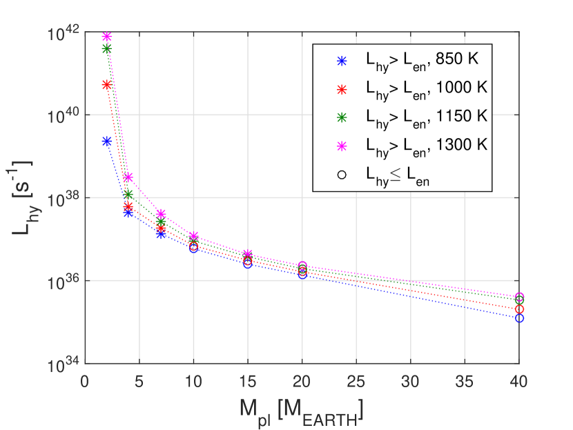
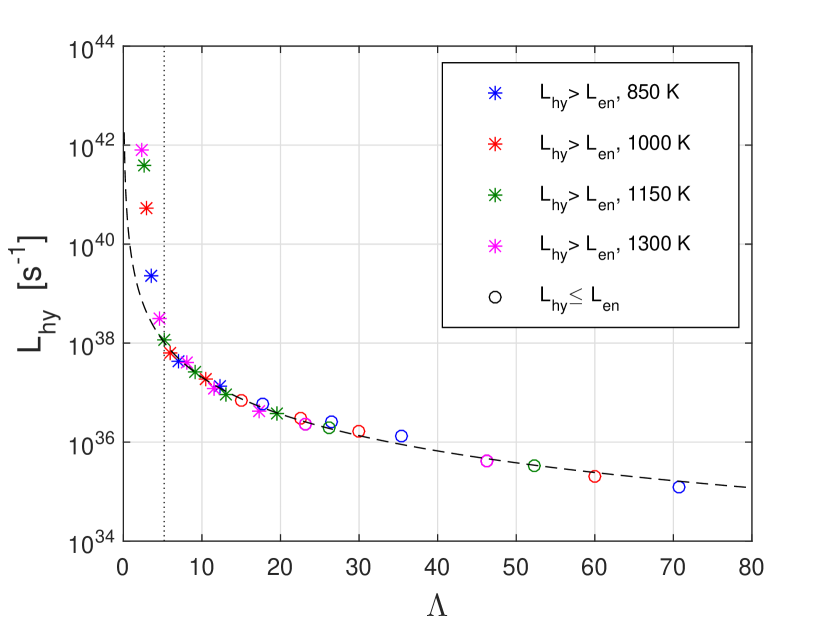
Figure 1: Hydrodynamic escape rates $L_{hy}$ as a function of planetary mass (top) and restricted Jeans escape parameter $\Lambda$ (bottom). Asterisks and circles mark models for which $L_{\rm hy}$ is higher and lower, respectively, than that estimated from the energy-limited formulation (see Section 4.1, for details). The dashed line in the bottom panel denotes Eq. (21). The vertical dotted line indicates the minimum $\Lambda$ value for which Eq. (21) is valid.

3 Results

3.1 Escape rates

For each cell in the model grid, we calculate the properties of the upper atmosphere including temperature, number density, and bulk flow velocity as a function of radial distance. From these quantities, we estimate the hydrodynamic hydrogen escape rate $L_{\rm hy}$ as the flow of particles through the upper boundary

$$L_{\rm hy}=4\pi R_{\rm roche}^{2}n_{1}V_{1}\,,$$ (17)

where $n_{1}$ and $V_{1}$ are the number density and velocity at the Roche radius $R_{\rm roche}$. Figure 1 shows the values of $L_{\rm hy}$ obtained from the simulations as a function of planetary mass and restricted Jeans escape parameter

$$\Lambda=\frac{GM_{\rm pl}m_{\rm H}}{k_{\rm B}T_{\rm eq}R_{\rm pl}}\,.$$ (18)

This last quantity corresponds to the value of the Jeans escape parameter calculated for the observed planetary radius and mass for the planet’s equilibrium temperature, and considering atomic hydrogen (Fossati et al. 2017). This parameter is particularly useful because it gives a rough measure of the planetary gravitational potential versus the intrinsic planetary thermal energy (i.e. excluding XUV heating), and hence it allows us to estimate the stability of the atmosphere against its own thermal energy and planetary gravity. The physical properties of the modelled planets and the derived escape rates are listed in Table $3$.

As expected, the escape rates increase with decreasing planetary mass. At high mass (i.e. $M_{\rm pl}$ $>$ 10 $M_{\oplus}$), the escape is driven by the heating caused by the absorption of the stellar XUV flux and the atmosphere is in the blow-off regime. Heating caused by absorption of the stellar X-ray flux contributes just a few percent of the total escape rates. For lower masses, where $L_{\rm hy}$ increases steeply, the escape is driven mostly by the planetary high thermal energy and low gravity. For these planets, the atmosphere lies in the boil-off regime (see Section 4.1).

3.2 Temperature and velocity profiles

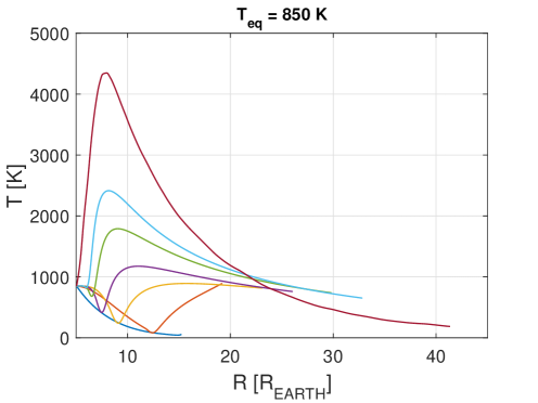
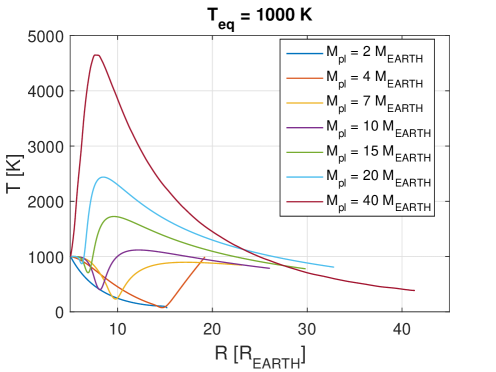
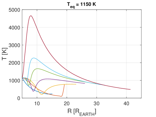
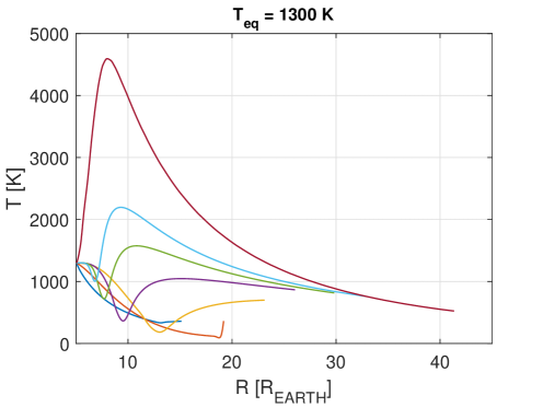
Figure 2: Temperature profiles of the modelled planets as a function of planetary mass and equilibrium temperature. For planets with a mass between 7 and 15 $M_{\oplus}$, the temperature profile presents a minimum close to $R_{\rm pl}$.

The atmospheric temperature profiles are mostly dependent on the planetary mass, while the adopted $T_{\rm eq}$ value has only a small influence (Fig. 2). For $M_{\rm pl}>10M_{\oplus}$ the models present efficient heating, with pronounced maxima, caused by the absorption of the stellar XUV radiation. For the lowest mass planets, the temperature profile is dominated by adiabatic cooling, driven by the strong hydrodynamic expansion of the atmosphere in the boil-off regime. For planets with intermediate masses (i.e. 7–15 $M_{\oplus}$), the temperature profile presents a minimum close to $R_{\rm pl}$, the position and amplitude of which decrease with increasing mass. We discuss the origin of this temperature minimum in Section 4.

For atmospheres dominated by adiabatic cooling, the temperature decreases at approximately the same rate throughout the atmosphere, independently of $T_{\rm eq}$. For the profiles presenting XUV heating in the atmosphere, the value of the maximum temperature increases slightly with decreasing temperature, with a difference of about 250 K between the coolest and hottest temperature maxima.

As stated in Section 2, the planetary atmosphere at the lower boundary consists of pure molecular hydrogen. Due to the XUV irradiation, hydrogen dissociates not far from the planetary surface and the upper part of the atmosphere is thus dominated by atomic hydrogen. The position of the dissociation barrier, the thickness of the hydrostatic $\rm H_{2}$ layers, and the atmospheric temperature mainly depend on the planetary mass. The dissociation appears to be more effective for the more massive planets, where the stellar flux penetrates deeper into the planetary atmosphere. Furthermore, the thickness of the pure molecular hydrogen layers (i.e. where the other species contribute less than 1%) varies with planetary mass and equilibrium temperature. For $T_{eq}=850$ K, the thickness of these layers ranges between 1.3 $R_{\rm pl}$ for the lowest mass planets to 0.04 $R_{pl}$ for the highest mass planets. By increasing the equilibrium temperature from the lowest to the highest value, the thickness of the molecular hydrogen layer increases by about 30%.

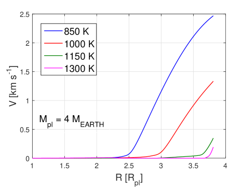
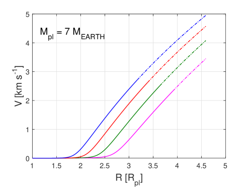
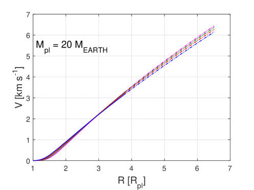
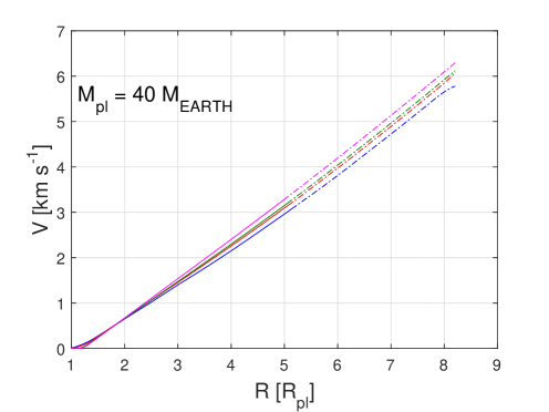
Figure 3: Gas velocity profiles for the planets with masses of 4 (top-left), 7 (top-right), 20 (bottom-left), and 40 (bottom-right) $M_{\oplus}$. The velocity profiles for planets with 10 and 15 $M_{\oplus}$ are very similar to those of the 20 $M_{\oplus}$ planet. The colours correspond to different values of the equilibrium temperature (blue: 850 K; red: 1000 K; yellow: 1150 K; magenta: 1300 K). The line style indicates whether a certain velocity is below (solid) or above (dash-dotted) the local sound speed.

Figure 3 shows the velocity profiles obtained for the modelled planets. For the lowest mass planets, the bulk of the atmosphere moves at a subsonic speed, with the local sound speed being $V_{\rm T}=\sqrt{k_{\rm B}T/m_{\rm H}}$. For the other planets, the upper part of the atmosphere becomes supersonic above the position of the maximum temperature. Similar to the behaviour observed for the temperature profiles, the position at which the atmosphere becomes supersonic gets closer to $R_{\rm pl}$ as the mass increases. The sensitivity of both temperature and velocity profiles to variations in $T_{\rm eq}$ decreases significantly with increasing mass: $T_{\rm eq}$ only seems to play a role in shaping the atmospheric profiles for the lower mass planets, for which the atmosphere is in the boil-off regime.

4 Discussion

4.1 Atmospheric escape regime

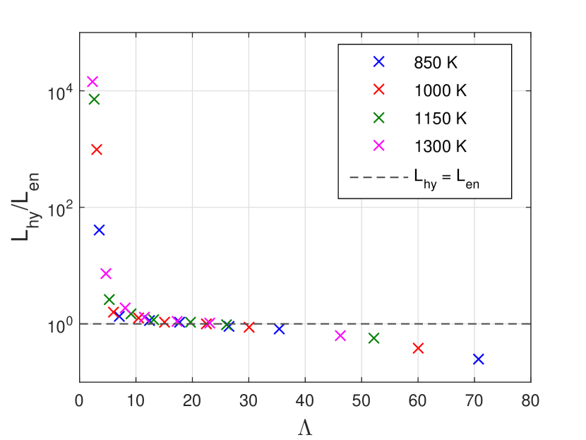
Figure 4: Ratio between the escape rates calculated with the hydrodynamic model $L_{\rm hy}$ and with the energy limited formulation $L_{\rm en}$ as a function of the restricted Jeans escape parameter $\Lambda$. The dashed horizontal line indicates the equality between $L_{\rm hy}$ and $L_{\rm en}$. The symbols are colour-coded as in the top panel and Fig. 1.

We compare here the escape rates derived from the models with those estimated through the energy-limited formulation (Watson et al. 1981; Erkaev et al. 2007)

$$L_{\rm en}=\frac{R_{\rm pl}R_{\rm eff}^{2}F_{\rm XUV}}{GM_{\rm pl}K}\,,$$ (19)

where $F_{\rm XUV}$ is the stellar XUV flux incident on the planet, $R_{\rm eff}$ is the radius at which most of the XUV flux is absorbed, and $K$ is a term accounting for Roche lobe effects (Table $3$). The value of $R_{\rm eff}$ is calculated as

$$R_{\rm eff}=R_{\rm pl}\sqrt{1+2\int_{1}^{\infty}{\left(1-\frac{J_{\rm XUV}(r,\frac{\pi}{2})}{F_{\rm XUV}}\right)r}dr}\,.$$ (20)

In Eq. (20), $J_{\rm XUV}$ corresponds to the stellar XUV flux inside the atmosphere, which depends on $r$ and on the spherical angle (see Erkaev et al. 2007, 2015, for more details). The $R_{\rm eff}$ values correspond roughly to the positions of the temperature maxima shown in Fig. 2 and hence $R_{\rm eff}$ increases with decreasing $\Lambda$. For the lowest mass planets, where the temperature decreases adiabatically, $R_{\rm eff}$ lies instead above the Roche radius, which is the upper boundary of our calculations. For such planets, we therefore consider $R_{\rm eff}$ to be equal to $R_{\rm roche}$, hence slightly underestimating the $L_{\rm en}$ values.

Figure 4 shows the $L_{\rm hy}$/$L_{\rm en}$ ratio as a function of $\Lambda$. This plot indicates that for $\Lambda$ values ranging between 10 and 40, the two escape rates are roughly similar, while for lower $\Lambda$ the escape rates calculated using the hydrodynamic model are significantly higher than those derived using Eq. (19). This agrees with the findings of Fossati et al. (2017), who carried out a similar analysis, but for 5 and 10 $M_{\oplus}$ planets subject to much smaller amounts (i.e. factor of 10 to 1000) of XUV irradiation. The atmospheres of planets with the lowest $\Lambda$ values lie therefore in the boil-off regime. This is also shown, for example, by the strong dependence of the escape rates on $T_{\rm eq}$ for these planets (see Fig. 1).

Given the monotonic increase of the escape rates with decreasing $\Lambda$, we fit the $L_{\rm hy}$ values with a logarithmic function of $\Lambda$, obtaining

$$\ln{L_{\rm hy}}=91.7-2.5\ln{\Lambda}\,,$$ (21)

where the fit was done excluding the planets for which $R_{\rm eff}$ lies above $R_{\rm roche}$. It is important to remark that this fit is valid just for planets with $\Lambda$ greater than about five and for the stellar parameters, including the XUV fluxes, adopted for these calculations. Higher or lower XUV fluxes would lead to higher or lower escape rates, respectively.

4.2 Impact of the uncertainties of the stellar parameters

As mentioned in Section 2.1, there is a significant difference in the stellar mass estimated by David et al. (2016) and Mann et al. (2016). This study is based on the stellar mass of 0.56 $M_{\odot}$ derived by Mann et al. (2016) and we discuss here the impact of this choice on the results. We re-calculated the grid of planetary upper atmosphere models considering a stellar mass of 0.3 $M_{\odot}$ (David et al. 2016). We found that, because of the decreased gravitational influence of the star on the planet, hence of the larger planetary Roche lobe, the escape rates for the lower mass planets are about half of those obtained considering the higher mass star. For the higher mass planets, instead, the modification of the gravitational potential has no effect on the escape rates.

The lower stellar mass leads also to lower stellar XUV fluxes. This is due to the dependence of the X-ray luminosity on the stellar mass, such that $L_{\rm X,0.56}\approx 1.8L_{\rm X,0.3}$, where the subscript indicates the stellar mass. Thus, when considering the lower stellar mass, the escape rates decrease by about 36% compared to those derived considering the higher stellar mass.

A further, closely related, uncertainty is that of the stellar bolometric luminosity, which enters also in the calculation of the XUV fluxes. By considering for example the estimate of $L_{\rm bol}$ based on the stellar age (Preibisch & Feigelson 2005), the XUV fluxes would increase by a factor of two. This would in turn lead to an increase of 40% in the escape rates for the most massive planets. These considerations indicate that the major uncertainties in the stellar parameters lead to escape rates that are within a factor of two of those presented in Section 3.

4.3 Possible impact of the modelling formalism

We discuss here how the results depend on the major modelling assumptions. One dimensional models are widely used for exoplanet studies, particularly with respect to upper atmosphere modelling (see e.g. Murray-Clay et al. 2009; Shaikhislamov et al. 2014; Salz et al. 2016; Erkaev et al. 2016, 2017; Fossati et al. 2017; Lammer et al. 2016). An upgrade to 2D or 3D simulations is instead required to model the interaction between the expanding planetary atmosphere with the stellar wind, particularly when considering ion pick-up processes related to planetary atmospheric escape. The mass loss expected to occur because of charge exchange processes is, however, about an order of magnitude smaller than the escape caused by XUV heating (see e.g. Kislyakova et al. 2014), and hence does not significantly affect our results. Furthermore, the stellar wind does not play a significant role if the planetary outflow is supersonic before the stellar-planetary interaction occurs, because the stellar wind particles do not penetrate into the deeper atmospheric layers. This is the case of K2-33b, except possibly for the lowest considered masses. However, for these cases, the planetary atmosphere fully escapes within 5 Myr.

The presence of strong transversal planetary winds would redistribute the thermal energy in the lower atmosphere from the day to the night side, thus lowering the temperature at the lower boundary of our simulations. Given the small dependence of our results on the planetary equilibrium temperature, we expect that a lower temperature by a few hundred degrees would not significantly affect our results.

As was stated in Section 2.2, we assume solar metallicity when estimating the lower pressure boundary $P_{0}$. We can therefore consider the effect of a different metallicity varying the lower pressure boundary. We thus conducted additional runs assuming a metallicity of 10$\times$ and 0.1$\times$ solar. We found that, at a temperature of 850 K, the escape rates change by about 5% in the case of the $M_{\rm pl}=20M_{\oplus}$ planet and by about 15% in the case of 7 $M_{\oplus}$ planet. Other, more local, parameters, such as temperature profiles, ionization rate, and position of the dissociation barrier, vary within 1%.

Finally, we tested the effect of the choice of chemical reaction rates. We ran further tests on the two simulated planets mentioned above (T${}_{\rm eq}=850$ K; M${}_{\rm pl}=7$ and $20M_{\oplus}$) substituting the reaction rates given by Yelle (2004) (used in this work) with those provided by the UMIST Database for Astrochemistry (UDfA) (http://udfa.ajmarkwick.net). We found that the escape rates vary by less than 0.5%, with the largest variations (still below 5%) being for the ionization rate.

4.4 Evolutionary status

We discuss here whether the derived escape rates, together with the age of the system, can provide any constraint on the planet’s minimum mass. We do not aim to realistically trace the evolution of the planet’s atmosphere, which would require more sophisticated models. We aim instead at providing an order of magnitude estimation for the timescale expected for the complete escape of a hydrogen-dominated atmosphere. By comparing it with the system’s age, we derive an estimate of the possible minimum planetary mass. To this end, one needs to assume a value for the current envelope mass fraction $f$, which is unknown. In the literature, the maximum $f$ value that is commonly considered is 50% (e.g. Rogers et al. 2011; Mordasini et al. 2012; Owen & Wu 2016). We therefore consider possible envelope mass fractions of 50%, 30%, 10%, and 1%. Given also the weak dependence of the escape rates on the equilibrium temperature, we consider the results obtained for a $T_{\rm eq}$ value of 850 K.

Figure 5 shows the timescale estimated for the complete escape of a hydrogen-dominated atmosphere (i.e. ratio between atmospheric mass and mass-loss rate) as a function of planetary mass, for the four considered $f$ values. This plot shows that, if the planet had a mass smaller than 7 $M_{\oplus}$, the planetary hydrogen-dominated envelope would have completely escaped by now. However, such a low planetary mass would imply a low bulk density, and therefore the presence of a thick hydrogen-dominated atmosphere, which is in contradiction with the previous statement. The result is that the planet cannot be less massive than 7 $M_{\oplus}$, regardless of the considered envelope mass fraction. In the same way, if the planet has an $f$ value smaller than 30% (or 10%), one could also safely exclude planetary masses smaller than 10 $M_{\oplus}$ (or 15 $M_{\oplus}$). For masses larger than 15–20 $M_{\oplus}$, the planet would keep its hydrogen-dominated atmosphere, even considering small envelope mass fractions, hence ending up as a hot Neptune.

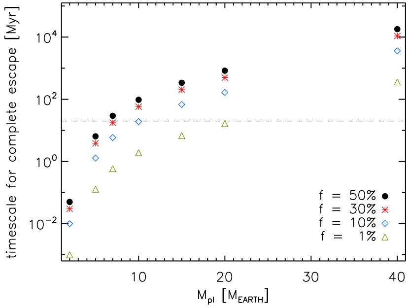
Figure 5: Timescale, in Myr, estimated for the complete escape of a hydrogen-dominated atmosphere as a function of planetary mass, assuming four different values of the atmospheric mass fraction $f$ of 50% (black dot), 30% (red asterisk), 10% (blue diamond), and 1% (green triangle). The horizontal dashed line indicates the maximum age (i.e. 20 Myr) derived for the K2-33 system (Mann et al. 2016).

These estimates do not consider that the stellar XUV flux, hence the atmospheric escape rates, will decrease with time. This will lead to a slight decrease of the possible minimum mass. To conclude, we can safely exclude the possibility that K2-33b is less massive than 7 $M_{\oplus}$, or 10 $M_{\oplus}$ if the envelope mass fraction is below 30%.

4.5 Temperature minima

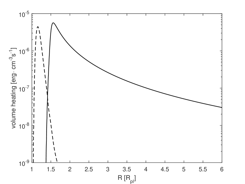
Figure 6: Volume heating rates of EUV (solid) and X-ray (dashed) stellar radiation for the 10 $M_{\oplus}$ planet with an equilibrium temperature of 850 K.

As mentioned in Section 3, the structure of the temperature profiles shown in Fig. 2 for planets with masses between 7 and 15 $M_{\oplus}$ is particularly unusual. To understand the origin of the temperature minima, we look at the effects of $\rm H_{3}^{+}$ cooling, X-ray heating, and EUV heating.

4.5.1 $\rm H_{3}^{+}$ cooling

Interestingly, most of the cooling caused by $\rm H_{3}^{+}$ molecules is located close to the position at which the temperature minimum occurs. We therefore ran simulations for the 10 $M_{\oplus}$ planet without considering $\rm H_{3}^{+}$ cooling, obtaining results that were not appreciably different from those of the original runs with the inclusion of $\rm H_{3}^{+}-$cooling. This result is in agreement with those of Shaikhislamov et al. (2014) and Chadney et al. (2015) who did similar tests for close-in Jupiter-mass planets.

4.5.2 X-ray heating

The X-ray heating rate is comparable to that produced by EUV, but, because of the much smaller absorption cross-section ($\sigma_{\rm X}\sim 0.5\times 10^{-3}\sigma_{\rm EUV}$), the X-rays penetrate significantly deeper into the atmosphere and deposit their energy in a thin layer where the atmosphere is dominated by $\rm H_{2}$ molecules (Fig. 6). Already at 1.5 $R_{\rm pl}$, X-ray heating becomes negligible compared to that produced by the EUV. Additional models run without the inclusion of the stellar X-ray fluxes show that X-ray heating is not responsible for the temperature minima either.

4.5.3 EUV heating

We further explored the effects of the intense EUV flux on the temperature profiles by carrying out additional simulations with the EUV fluxes reduced by a factor of 100 and 1000, compared to what we estimated for K2-33. We found that the amplitude of the minimum decreases in the first case and vanishes completely in the second.

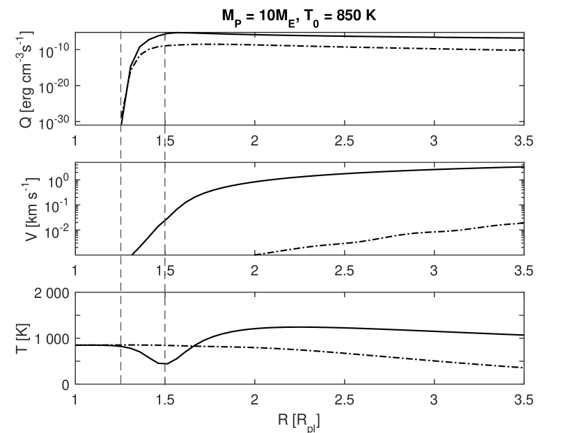
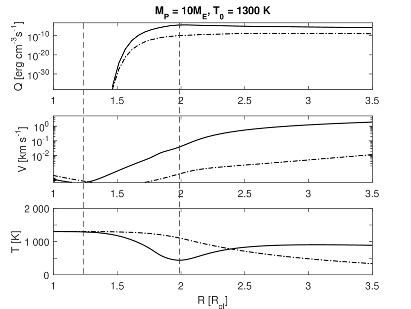
Figure 7: Top three panels: EUV volume heating rate (top), bulk velocity (middle), and temperature (bottom) profiles for the 10 $M_{\oplus}$ planet with an equilibrium temperature of 850 K. The solid line is for the planet irradiated by the XUV flux estimated for K2-33 and the dash-dotted line is for the same planet, but with a 1000 times weaker level of XUV irradiation. The vertical dashed lines mark the position at which the velocity begins to rise (left) and that of the temperature minimum for the most irradiated planet (right). Bottom three panels: same as the top three panels, but for a planet with an equilibrium temperature of 1300 K. For the lower and higher temperature planets, $R_{\rm eff}$ lies at about 2.3 and 3.0 $R_{\rm pl}$, respectively.

Figure 7 shows the atmospheric profiles for temperature, velocity, and EUV volume heating rate for the planets with a mass of 10 $M_{\rm\bigoplus}$ and an equilibrium temperature of 850 and 1300 K. For each planet, we ran two simulations: one considering the EUV flux estimated for K2-33, and one considering the same EUV flux reduced by a factor of 10³. In all cases, the atmospheres are characterized by adiabatic cooling close to R_pl, but only the planets subject to the stronger EUV irradiation present a temperature minimum close to the position of the peak of the volume heating rate.

The observed temperature minima are therefore caused by the extreme EUV heating. For the more irradiated planets, the EUV heating rate is about five orders of magnitude higher than that of the less irradiated planets, which also leads to the formation of a hydrodynamic flow much closer to $R_{\rm pl}$. This results in a strong adiabatic cooling caused by the fast gas flow, which leads to a local decrease in the temperature. However, when the heating reaches values of about 1.5–3$\times$10^-6 erg cm^-3 s^-1, it dominates the adiabatic cooling, producing the observed temperature minimum.

5 Conclusions

The young K2-33b planet offers the unique opportunity to study the very early phases of planetary evolution at a time when the planetary atmosphere is subject to extremely intense high-energy stellar fluxes. This is therefore the time when atmospheric escape is strongest and shapes the planetary envelope, setting it onto its final evolutionary path. We employed an upper atmosphere hydrodynamic model to study the physical characteristics of the planetary envelope and infer the escape rates. In order to more adequately model such a young system, we included in the model X-ray heating and $\rm H_{3}^{+}$ cooling, in addition to the processes included in the model in previous studies (Erkaev et al. 2016). In the absence of a measured planetary mass, we consider masses ranging between 2 and 40 $M_{\oplus}$, while the planetary radius was kept fixed to the measured value.

We found that for values of the restricted Jean escape parameter $\Lambda$ smaller than 10, the escape rates are considerably larger than those derived from the energy-limited formula. For these planets, the escape is driven by the high intrinsic thermal energy of the atmosphere and low planetary gravity, while XUV heating plays a negligible role. For planets with a $\Lambda$ value between 10 and 40, the hydrodynamic escape rates are comparable to those provided by the energy limited formula, while for larger $\Lambda$ values they are lower.

For the lowest mass planets, the temperature profile is characterized by adiabatic cooling, caused by the strong hydrodynamic outflow of the atmosphere. For the highest mass planets, the temperature profiles present a maximum close to the position of maximum absorption of the stellar EUV flux (we find that X-ray heating plays a negligible role compared to EUV heating). For the intermediate mass planets, we find instead the presence of a local minimum close to the planetary radius. Additional dedicated simulations showed that this feature is caused by the combination of adiabatic cooling and the absorption of the strong stellar EUV fluxes.

Finally, we roughly estimate whether the derived escape rates, together with the age of the system, can provide any constraint on the minimum mass possible for the planet. We found that for masses smaller than 7 $M_{\oplus}$, the planet would have completely lost its hydrogen-dominated envelope, which is in contradiction with the low average density that would result from a low planetary mass. We therefore place a lower limit of 7 $M_{\oplus}$ on the planetary mass.

Table 2: Reactions and relative cross-sections employed in the model.

$H\rightarrow H^{+}+e$	$\nu_{H}=5.9\times 10^{-8}\phi_{EUV}s^{-1}$	Storey & Hummer (1995)
$\rm H_{2}\rightarrow\rm H_{2}^{+}+e$	$\nu_{\rm H_{2}}=3.3\times 10^{-8}\phi_{EUV}s^{-1}$	Murray-Clay et al. (2009)
$H^{+}+e\rightarrow H$	$\alpha_{H}=4\times 10^{-12}(300/T)^{0.64}cm^{3}s{-1}$	Yelle (2004)
$\rm H_{2}^{+}+e\rightarrow H+H$	$\alpha_{\rm H_{2}}=2.3\times 10^{-8}(300/T)^{0.4}cm^{3}s^{-1}$	Yelle (2004)
$\rm H_{2}\rightarrow H+H$	$\nu_{diss}=1.5\times 10^{-9}e^{(-49000/T)}$	Yelle (2004)
$H+H\rightarrow\rm H_{2}$	$\gamma_{H}=8.0\times 10^{-33}(300/T)^{0.6}$	Yelle (2004)
$H+e\rightarrow H^{+}$	$\nu_{Hcol}=5.9\times 10^{-11}T^{1/2}e^{(-157809/T)}$	Black (1981)
$\rm H_{2}^{+}+\rm H_{2}\rightarrow\rm H_{3}^{+}+H$	$\gamma_{\rm H_{2}}=2\times 10^{-9}$	Yelle (2004)
$\rm H_{3}^{+}+H\rightarrow\rm H_{2}^{+}+\rm H_{2}$	$\gamma_{\rm H_{2}}=2\times 10^{-9}$	Yelle (2004)
$\rm H_{3}^{+}+e\rightarrow\rm H_{2}+H$	$\alpha_{\rm H_{3}^{+}1}=2.9\times 10^{-8}(\frac{300}{T_{e}})^{0.65}$	Yelle (2004)
$\rm H_{3}^{+}+e\rightarrow H+H+H$	$\alpha_{\rm H_{3}^{+}2}=8.6\times 10^{-8}(\frac{300}{T_{e}})^{0.65}$	Yelle (2004)

Table 3: Physical properties of the modelled planets and escape and mass-loss rates derived from the simulations. The mass-loss rates are given in $g\,s^{-1}$ and in $M_{\oplus}\,Gyr^{-1}$.

$M_{\rm pl}$	$T_{\rm eq}$	$\Lambda$	$L_{\rm hy}$	$L_{\rm en}$	$\dot{M}_{\rm hy}$	$\dot{M}_{\rm en}$	$\dot{M}_{\rm hy}$	$\dot{M}_{\rm en}$	$R_{\rm roche}$	$R_{\rm eff}$
$[M_{\oplus}]$	[K]		$[10^{35}s^{-1}]$	$[10^{35}s^{-1}]$	$[10^{11}gs^{-1}]$	$[10^{11}gs^{-1}]$	$[M_{\oplus}Gyr^{-1}]$	$[M_{\oplus}Gyr^{-1}]$	$[R_{\rm pl}]$	$[R_{\rm pl}]$
$2.0$	$850$	$3.5$	$22654.8$	$585.1$	$37892.4$	$978.6$	$20008.9$	$516.7$	$3.02$	$3.02$
$4.0$	$850$	$7.1$	$440.4$	$346.8$	$736.6$	$580.0$	$389.0$	$306.3$	$3.81$	$3.29$
$7.0$	$850$	$12.4$	$134.7$	$126.1$	$225.3$	$210.8$	$119.0$	$111.3$	$4.59$	$2.62$
$10.0$	$850$	$17.7$	$58.7$	$59.6$	$98.3$	$99.6$	$51.9$	$52.6$	$5.17$	$2.16$
$15.0$	$850$	$26.5$	$25.0$	$29.3$	$41.8$	$49.0$	$22.1$	$25.9$	$5.92$	$1.85$
$20.0$	$850$	$35.3$	$13.6$	$17.8$	$22.8$	$29.8$	$12.0$	$15.7$	$6.51$	$1.67$
$40.0$	$850$	$70.7$	$1.3$	$4.7$	$2.1$	$7.9$	$1.1$	$4.2$	$8.20$	$1.21$
$2.0$	$1000$	$3.0$	$536878.1$	$585.3$	$897982.4$	$979.0$	$474176.6$	$517.0$	$3.02$	$3.02$
$4.0$	$1000$	$6.0$	$618.6$	$418.4$	$1034.6$	$699.8$	$546.3$	$370.0$	$3.81$	$3.61$
$7.0$	$1000$	$10.5$	$186.7$	$156.8$	$312.3$	$262.3$	$164.9$	$138.5$	$4.59$	$2.93$
$10.0$	$1000$	$15.0$	$69.8$	$70.4$	$116.7$	$117.8$	$61.6$	$62.2$	$5.17$	$2.35$
$15.0$	$1000$	$22.5$	$30.8$	$33.1$	$51.5$	$55.4$	$27.2$	$29.2$	$5.92$	$1.97$
$20.0$	$1000$	$30.0$	$16.4$	$19.8$	$27.4$	$33.0$	$14.5$	$17.4$	$6.51$	$1.76$
$40.0$	$1000$	$60.1$	$2.0$	$5.7$	$3.4$	$9.6$	$1.8$	$5.0$	$8.20$	$1.34$
$2.0$	$1150$	$2.6$	$3950771.2$	$585.3$	$6608059.9$	$979.0$	$3489363.6$	$517.0$	$3.02$	$3.02$
$4.0$	$1150$	$5.2$	$1184.9$	$462.4$	$1981.8$	$773.5$	$1046.5$	$408.4$	$3.81$	$3.80$
$7.0$	$1150$	$9.1$	$267.2$	$192.7$	$446.9$	$322.4$	$236.0$	$170.2$	$4.59$	$3.24$
$10.0$	$1150$	$13.1$	$90.6$	$82.6$	$151.6$	$138.1$	$80.1$	$72.9$	$5.17$	$2.54$
$15.0$	$1150$	$19.6$	$37.8$	$37.3$	$63.1$	$62.3$	$33.3$	$32.9$	$5.92$	$2.09$
$20.0$	$1150$	$26.1$	$19.5$	$21.8$	$32.6$	$36.5$	$17.2$	$19.3$	$6.51$	$1.84$
$40.0$	$1150$	$52.2$	$3.4$	$6.4$	$5.7$	$10.7$	$3.0$	$5.6$	$8.20$	$1.41$
$2.0$	$1300$	$2.3$	$7864357.0$	$585.3$	$13153923.0$	$979.0$	$6945884.8$	$517.0$	$3.02$	$3.02$
$4.0$	$1300$	$4.6$	$3149.0$	$464.3$	$5267.1$	$776.7$	$2781.3$	$410.1$	$3.81$	$3.81$
$7.0$	$1300$	$8.1$	$407.8$	$230.2$	$682.1$	$385.0$	$360.2$	$203.3$	$4.59$	$3.55$
$10.0$	$1300$	$11.6$	$118.2$	$96.8$	$197.8$	$161.8$	$104.4$	$85.5$	$5.17$	$2.75$
$15.0$	$1300$	$17.3$	$42.9$	$41.9$	$71.7$	$70.1$	$37.9$	$37.0$	$5.92$	$2.22$
$20.0$	$1300$	$23.1$	$23.0$	$24.0$	$38.5$	$40.2$	$20.3$	$21.2$	$6.51$	$1.94$
$40.0$	$1300$	$46.2$	$4.1$	$6.9$	$6.8$	$11.6$	$3.6$	$6.1$	$8.20$	$1.47$