Stirring a black hole

Abstract

We present novel asymptotically global AdS₄ solutions, constructed by turning on a dipolar differential rotation at the conformal boundary. At fixed energy and boundary profile, we find two different geometries: a horizonless spacetime, and a deformed, hourglass shaped black hole with zero net angular momentum. Both solutions exist up to some maximum amplitudes of the boundary profile, and develop an ergoregion attached to the boundary before the maximum amplitude is reached. We show that both spacetimes develop hair as soon as the ergoregion develops. Furthermore, we discuss the full phase diagram, including the possibility of phases with disconnected horizons, by considering the Mathisson-Papapetrou equations for a spinning test particle. Finally, we provide a first principle derivation of the superradiant bound purely from CFT data, and outline possible scenarios for the late time evolution of the system.

1 Introduction

The behaviour of quantum field theories (QFTs) on a fixed curved spacetime is largely unknown territory, posing both conceptual and technical challenges. Perhaps the only known universal phenomenon is the emission of Hawking radiation around asymptotically flat black holes, and its concomitant information paradox Hawking:1974rv . However, even in the absence of horizons, interesting novel phenomenology can arise when considering quantum field theory on curved spacetimes, such as vacuum polarisation or particle production.

Much of our current understanding of QFTs on fixed nontrivial backgrounds comes from perturbation theory. The reasons for this are twofold: we do not know how to analytically study generic strongly coupled theories and we do not yet have a lattice formulation for a QFT on a generic curved spacetime. This in turn implies that questions that involve strongly coupled phenomenology, such as confinement, are out of reach and might bring novel effects. The gauge/gravity duality Maldacena:1997re ; Gubser:1998bc ; Witten:1998qj ; Aharony:1999ti offers a unique opportunity to study such scenarios.

The gauge/gravity duality maps a class of $d-$dimensional string theories with anti de-Sitter boundary conditions (AdS), to certain non-gravitational conformal quantum field theories (CFTs) formulated in $\tilde{d}$ dimensions, with $\tilde{d}<d$. CFTs typically come with two parameters: a dimensionless coupling $\lambda$ which measures the interaction of the microscopic constituents of the theory, and a measure of its degrees of freedom, which we will denote by $N$. One of the realisations in Maldacena:1997re was the fact that in the limit where $\lambda\to+\infty$ and $N\to+\infty$, the corresponding string theory duals become classical supergravity theories. This is precisely the regime where the dual CFT becomes strongly coupled, and where we expect interesting new phenomena to arise.

A seemingly unrelated topic is that of superradiance, the study of which was pioneered by Zeldovich:1971 ; Zeldovich:1972 ; Press:1972zz ; Starobinsky:1973scalar ; Starobinsky:1973 ; Detweiler:1973zz ; Zouros:1979iw ; Detweiler:1980uk in the asymptotically flat context, and the first quantitative study involving rotating black holes in AdS featured in Kunduri:2006qa ; Dias:2011at ; Dias:2013sdc ; Cardoso:2013pza . The idea behind the so called superradiant instability is simple: rotating black holes in AdS with sufficient angular velocity $\Omega_{H}$ can have ergoregions, which can act as reservoirs for negative energy if waves with azimuthal quantum number $m$ and frequency $0<\omega<m\,\Omega_{H}$ are scattered. If a rotating black hole with an ergoregion is surrounded by a confining potential (in our case this is provided by the AdS potential, but it could be equally provided by a mass term Detweiler:1973zz ; Herdeiro:2014goa for asymptotically flat spacetimes), then this process will be recurrent and will eventually lead to an instability. The endpoint of this instability seems to be outside the scope of current numerical methods in AdS, however, in Dias:2011at ; Dias:2015rxy ; Niehoff:2015oga it has been argued that the instability is likely to lead to a pointwise violation of the weak cosmic censorship conjecture in AdS.

One might have expected superradiance to produce an interesting phase diagram for CFTs in compact spacetimes, via the gauge/gravity duality. While this is certainly true in the context of the microcanonical ensemble, the grand-canonical ensemble seems rather innocuous. The reason for this is that the region of moduli space unstable to superradiance is cloaked by a first order Hawking-Page phase transition Hawking:1982dh . This implies that, for a fixed temperature and angular velocity that render the Kerr-AdS black hole unstable, the preferred phase is that of thermal AdS!

We shall see that this is no longer the case if we consider nontrivial boundary metrics that have differential rotation. For each boundary profile metric, we find two classes of solutions: a solitonic horizonless spacetime and black hole solutions, which are schematically pictured in Fig. 1.

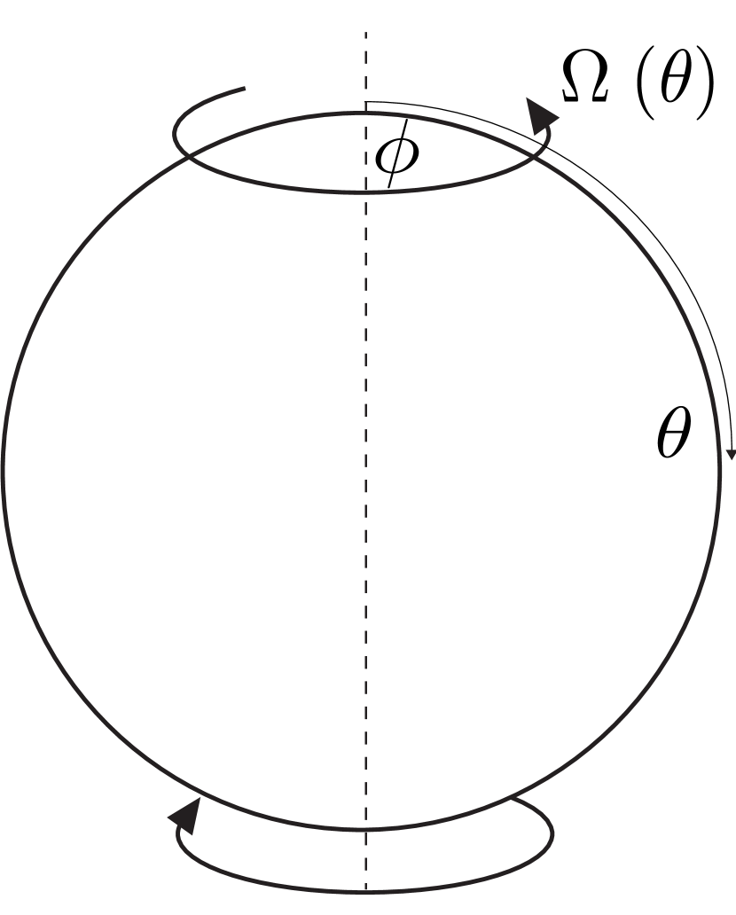
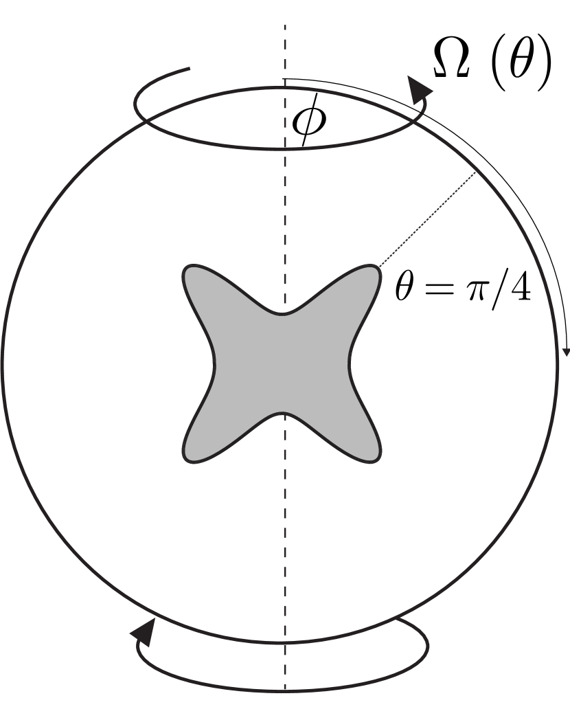
Figure 1: Illustration of the novel AdS₄ geometries. Left: Solitonic solutions with a differentially rotating boundary. Right: Black hole solutions. The rotational pull force is maximal at $\theta=\pi/4$, deforming the black hole horizon into an hourglass shape.

The solitonic solutions have no horizon, and correspond to deformations of global AdS₄, while black hole solutions can be seen as continuous deformations of Schwarzschild-AdS₄ black holes. We will find that both phases develop hair due to superradiance if the boundary deformation is sufficiently large. In addition, we shall see that the phase diagram of solutions is rather intricate, including certain regions of moduli space with up to six-fold degeneracy.

One might wonder about the interpretation of our results in terms of CFT data. We shall see that we will be able to reconstruct the critical value of the amplitude for which the system develops hair from pure CFT data. This will allow us to identify which CFT observables might be sensitive to this phenomenon and to the hypothetical violation of weak cosmic censorship in the bulk.

For simplicity, our work will focus on four-dimensional bulk physics and can easily be embedded into a full string theory embedding, as for instance in ABJM Aharony:2008ug . While some of what we describe might follow through to the higher-dimensional case, there are some important differences. For instance, for $d>4$, the Gregory-Laflamme instability might also play a role, and render some of our solutions unstable before they have a chance of becoming superradiant. We note however, that such an instability is also likely to lead to a violation of the weak cosmic censorship conjecture Lehner:2010pn ; Figueras:2015hkb ; Figueras:2017zwa . In this sense, we expect the relevant physics to be easier to dissect in $d=4$.

This paper is organised as follows. Section 3 details the construction of soliton and black hole solutions. In section 4 we present results, and carry out thermodynamical analysis. Section 5 presents stability analysis in which we consider a massless scalar field. Section 6 discusses the CFT interpretation of our results and attempts to identify the field theory variables that best describe it. In section 7, we study possible multi horizon equilibrium configurations for spinning test particles. Finally, in section 8, we briefly discuss the holographic dual of theories living on a fixed rotating background geometry containing no ergoregions. We conclude in section 9 with discussion and an outline for further work.

2 Setup

We start with the four-dimensional Einstein-Hilbert action supplemented by the Gibbons-Hawking-York boundary term York:1972sj ; Gibbons:1976ue :

$$S=\frac{1}{16\pi G_{N}}\int_{\small{\mathcal{M}}}\mathrm{d}^{4}x \sqrt{-g}\left(R[g]+\frac{6}{L^{2}}\right)+\frac{1}{8\pi G_{N}}\int_{\small{\partial\mathcal{M}}}\mathrm{d}^{3}x\sqrt{-\gamma}\,K,$$ (1)

where $\partial\mathcal{M}$ is the boundary of AdS₄, $\gamma_{\mu\nu}$ is the induced metric on the boundary, $K$ is the trace of the extrinsic curvature of the boundary, $L$ is the length scale of AdS₄ and $R[g]$ the Ricci scalar. The equations of motion derived from (1) read

$$R_{\mu\nu}+\dfrac{3}{L^{2}}g_{\mu\nu}=0,$$

and we are looking for asymptotically AdS₄ solutions, with a rotating conformal boundary given by

$$\mathrm{d}s^{2}_{\partial}=-\mathrm{d}t^{2}+\mathrm{d}\theta^{2}+\sin^{2}{\theta}\left[\mathrm{d}\phi+\Omega(\theta)\mathrm{d}t\right]^{2},$$ (2)

with a dipolar differential rotation profile $\Omega(\theta)=\varepsilon\cos{\theta}$. We will be interested in finding solutions where $\partial_{t}$ and $\partial_{\phi}$ extend as Killing fields into the bulk. Close to the poles and on the equator, $\partial_{t}$ is always timelike for any value of $\varepsilon$. However, its norm

$$\mathinner{\!\left\lVert\partial_{t}\right\rVert}^{2}=-1+\frac{\varepsilon^{2}}{4}\sin^{2}{2\theta}$$ (3)

is maximal at $\theta=\pi/4$, and $\partial_{t}$ becomes spacelike for certain regions of $\theta$ if ${\varepsilon>2}$. We shall see that both black holes and solitons develop hair due to superradiance if $\varepsilon>2$. One might wonder whether this could have been anticipate using the results of Green, Hollands, Ishibashi and Wald Green:2015kur . However, the theorems presented in Green:2015kur were deduced under the assumption that the boundary metric was metrically that of the Einstein static universe, which is not the case in our setup. Our results suggest that a generalisation of the results in Green:2015kur should exist even for nontrivial boundary metrics such as ours.

3 Numerical Construction

3.1 Numerical Method

To solve the Einstein equation we employ the DeTurck method Headrick:2009pv ; Wiseman:2011by (for a review see 2016CQGra..33m3001D ) where we instead solve the equivalent Einstein-DeTurck equation

$$R_{\mu\nu}+\dfrac{3}{L^{2}}g_{\mu\nu}-\nabla_{(\mu}\xi_{\nu)}=0,$$ (4)

where $\xi^{\mu}=g^{\nu\rho}\left(\Gamma^{\mu}_{\nu\rho}[g]-\Gamma^{\mu}_{\nu\rho}[\tilde{g}]\right)$ is the DeTurck vector and $\tilde{g}$ is an appropriate reference metric of our choice (as detailed in the following subsection). Provided that $\xi^{\mu}=0$, solutions to (4) will also be solutions of the Einstein equation. Fortunately, it has recently been shown that, for spacetimes possessing a $(t,\phi)\to-(t,\phi)$ reflection symmetry, solutions with $\xi\neq 0$ cannot exist Figueras:2016nmo - our spacetimes enjoy such a symmetry. We can thus monitor the norm of $\xi$ to provide a global measure of our numerical integration scheme (see Appendix A).

The DeTuck method has the advantage of rendering the equations elliptic, and conveniently fixing the gauge. We solve (4) using the Newton-Raphson method with pseudospectral collocation on a square half–half Chebyshev grid. Because our ansatz is written in such a way that all unknown functions are even about two of the grid edges (see the next subsection), we can halve the Chebyshev grid while effectively interpolating over the full grid. This in turn allows us to use a smaller grid size to achieve a desired numerical accuracy. Convergence of our solutions is presented in Appendix A (Fig. 21).

3.2 Ansätze

3.2.1 Soliton

In order to find solitonic solutions we consider the following numerical ansatz

$$\mathrm{d}s^{2}=\frac{L^{2}}{(1-y^{2})^{2}}\Bigg{\{}-Q_{1}\,\mathrm{d}t^{2}+\frac{4\,Q_{2}\,\mathrm{d}y^{2}}{2-y^{2}}+y^{2}(2-y^{2})\Bigg{[}\frac{4\,Q_{3}}{2-x^{2}}\left(\mathrm{d}x+\frac{x}{y}\sqrt{2-x^{2}}\,\,Q_{4}\,\mathrm{d}y\right)^{2}\\ +(1-x^{2})^{2}Q_{5}\,\left(\mathrm{d}\phi+yx\sqrt{2-x^{2}}\,Q_{6}\,\mathrm{d}t\right)^{2}\Bigg{]}\Bigg{\}}\,,$$ (5)

with $Q_{i}$, $i\in\{1,\ldots,6\}$, being functions of $(x,y)$. If $Q_{1}=Q_{2}=Q_{3}=Q_{5}=1$ and $Q_{4}=Q_{6}=0$, the line element (5) reduces to that of pure AdS₄ in global coordinates, with $y$ being related to the usual radial coordinate in AdS₄ via $r=L\,y\sqrt{2-y^{2}}/(1-y^{2})$, and $x$ parametrising the standard polar angle on $S^{2}$ with the identification $\sin\theta=1-x^{2}$. The powers of $y$ and $1-x^{2}$ appearing in the ansatz ensure that the metric is regular at the origin $y=0$ and axis of rotation $x=\pm 1$ for smooth functions $Q_{i}$.

The reference metric $\tilde{g}$ used in the DeTurck method is chosen by setting $Q_{6}=\varepsilon$, and $Q_{1}=Q_{2}=Q_{3}=Q_{5}=Q_{4}+1=1$, everywhere in the bulk. The parameter $\varepsilon$ controls the rotation on the boundary and in turn the stirring of the bulk.

As we are considering a dipolar problem we have reflection symmetry $x\to-x$ and thus both coordinates take values in the square domain $[0,1]\times[0,1]$. Because the functions $Q_{i}$ are constructed to be even around $x=0$ (the equator) and $y=0$ (the origin), we can use a square half–half Chebyshev grid clustering around the $x=1$ and $y=1$ boundaries and thus effectively interpolate the functions with half the number of points. This is especially advantageous as spectral convergence is exponential with grid size. In addition, it fixes smoothness of the geometry at the reflection boundary.

This leaves us with two boundaries, one at the conformal boundary located at $y=1$, and one at $x=1$. The latter is a physical boundary, whereas the former is a fictitious boundary where regularity must be imposed. Expanding the equations of motion near $x=1$ as a power series in $(1-x)$ gives $Q_{3}(1,y)=Q_{5}(1,y)$ and $Q_{4}(1,y)=0$, as well as $\partial_{x}Q_{1}=\partial_{x}Q_{2}=\partial_{x}Q_{3}=\partial_{x}Q_{4}=\partial_{x}Q_{5}=0$.

At the conformal boundary, we demand the metric (5) approaches global AdS₄ with a rotating conformal boundary metric, that is to say, we require

$$Q_{1}(x,1)=Q_{2}(x,1)=Q_{3}(x,1)=Q_{5}(x,1)=Q_{4}(x,1)+1=1\,,\quad\text{and}\quad Q_{6}(x,1)=\varepsilon\,.$$ (6)

Comparing the conformal boundary metric obtained from our boundary conditions (6) and (2), gives $\Omega(\theta)=\varepsilon\cos\theta$, in standard polar coordinates on $S^{2}$.

3.2.2 Black Holes

For the black hole solutions we use the ansatz

$$\mathrm{d}s^{2}=\frac{L^{2}}{(1-y^{2})^{2}}\Bigg{\{}-y^{2}\tilde{\Delta}(y)Q_{1}\mathrm{d}t^{2}+\frac{4\,y_{+}^{2}Q_{2}\,\mathrm{d}y^{2}}{\tilde{\Delta}(y)}+y_{+}^{2}\Bigg{[}\frac{4\,Q_{3}}{2-x^{2}}\left(\mathrm{d}x+x\sqrt{2-x^{2}}\,y\,Q_{4}\,\mathrm{d}y\right)^{2}\\ +(1-x^{2})^{2}Q_{5}\,\left(\mathrm{d}\phi+y^{2}x\sqrt{2-x^{2}}\,Q_{6}\,\mathrm{d}t\right)^{2}\Bigg{]}\Bigg{\}},$$ (7a)

where

$$\Delta(y)=(1-y^{2})^{2}+y_{+}^{2}(3-3y^{2}+y^{4})\,,\quad\text{and}\quad\tilde{\Delta}(y)=\Delta(y)\delta+y_{+}^{2}(1-\delta)\,,$$ (7b)

with $Q_{i}$, $i\in\{1,\ldots,6\}$, being functions of $(x,y)$. If $Q_{1}=Q_{2}=Q_{3}=Q_{5}=\delta=1$ and $Q_{4}=Q_{6}=0$, the line element (5) reduces to that of Schwarzschild-AdS₄ black hole in global coordinates, with $y$ being related to the usual radial coordinate via $r=L\,y_{+}/(1-y^{2})$, and $x$ parametrising the standard polar angle on $S^{2}$ with the identification $\sin\theta=1-x^{2}$.

The reference metric is chosen to have $Q_{6}=\varepsilon$ and, similarly to the soliton case, we work on a unit square grid. Regularity at $x=1$ demands $\partial_{x}Q_{i}(x,y)=0$ ($i\neq 4$), $Q_{4}(x,y)=0$, and $Q_{3}(x,y)=Q_{5}(x,y)$. At the conformal boundary, we set $Q_{i}(x,1)=1$ for $i=1,2,3,5$, $Q_{4}(x,1)=0$ and $Q_{6}(x,1)=\varepsilon$.

In the ansatz (7a) we have three parameters: $\varepsilon$, which sets the amplitude of the boundary rotation, and $(y_{+},\delta)$, which set the black hole temperature. The Hawking temperature is computed in the usual way by requiring smoothness of the Euclidean spacetime and is given by

$$T=\frac{(1-\delta)y_{+}^{2}+\delta\left(3y_{+}^{2}+1\right)}{4\pi y_{+}}.$$ (8)

For $\delta=1$, the temperature has a minimum at $y_{+}=1/\sqrt{3}$, coinciding with the minimal temperature of a Schwarzschild-AdS₄, occurring at $T_{\min}^{\mathrm{Schw}}\equiv\sqrt{3}/(2\pi)$. In general we will have two branches of solutions with the same temperature which we will refer to as large and small black holes. However, when $\varepsilon\neq 0$, our new deformed black holes can have a minimum temperature below that of the Schwarzschild-AdS₄ black hole. In order to bypass this, we introduced a parameter $\delta$ which allows us to get arbitrarily close to zero temperature. Computations with $T>T_{\min}^{\mathrm{Schw}}$ were performed using the ansatz where $\delta=1$, and the results with $\delta\neq 1$ enjoy similarly sufficient convergence properties as those with $\delta=1$ (see Appendix A).

4 Numerical Results

For simplicity of presentation, in all of our plots we will set $L=1$.

4.1 Soliton

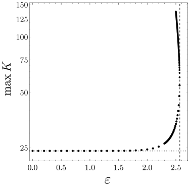
Figure 2: The log-linear plot of the maximum of the Kretschmann scalar against the rotation parameter for the soliton solutions. The dashed gridline marks $\varepsilon_{c}$, and the dotted line shows the $\max K=24/L^{4}$ for pure AdS₄.

One of the most interesting results of our manuscript is that we find no soliton solutions for $\varepsilon>\varepsilon_{c}\simeq 2.565$. In fact, we find no stationary axisymmetric solutions for $\varepsilon>\varepsilon_{c}$. Furthermore, there is a range $\varepsilon\in(2,\varepsilon_{c})$ in which two solitons exist for each value of $\varepsilon$, demonstrating non-uniqueness within the soliton family.

We have monitored the behaviour of the maximum of the Kretschmann scalar as a function of $\varepsilon$. Since we have no matter fields, besides a negative cosmological constant, the Kretschmann curvature invariant $K=R_{abcd}R^{abcd}$ is related to the norm of the Weyl tensor in a simple manner

$$L^{4}\,W_{abcd}W^{abcd}=L^{4}\,K-24\,,$$

that is to say, the local tidal forces scale like $K^{1/2}$.

The Kretschmann scalar $K$ is maximal at the equator $x=0$, and slowly deforms from the pure AdS₄ value of $24/L^{4}$ as we increase $\varepsilon\rightarrow\varepsilon_{c}$, forming two large extrema. The minima grows only slightly slower than the maxima, and the latter is plotted against $\varepsilon$ in Fig 2. For $\varepsilon>2$, we can see that two soliton solutions exist for a fixed value of $\varepsilon$. We call the upper branch the large branch, and the lower branch the small branch. The large branch of solitons smoothly extends the growth of $K$, which increases without bound, indicating formation of a curvature singularity. Also we note that for the soliton, the metric component $g_{tt}$ tends to zero at the origin, possibly as $\varepsilon\rightarrow 2$ from above.

4.2 Black Holes

4.2.1 The horizon geometry

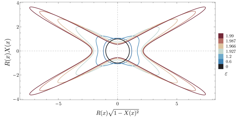
Figure 3: Hyperbolic embedding of the cross section of the black hole horizons, for several values of the parameter $\varepsilon$ and a fixed temperature $T=1/\pi$. As we increase $\varepsilon$, the arms of the horizon cross section get stretched further apart. This picture is qualitatively the same for $T\geq 1/\pi$.

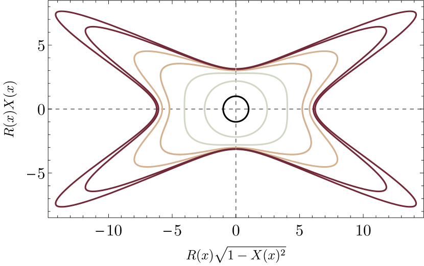
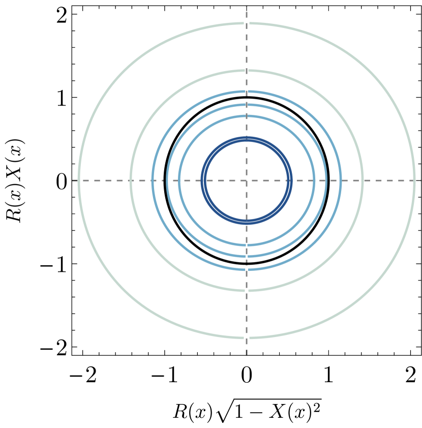
Figure 4: Hyperbolic embedding of the cross section of the black hole solution horizons, for several values of the parameter $\varepsilon$ and a fixed low temperature $T=0.2506$. In this regime, there is a four-fold black hole non-uniqueness. Left: Embeddings for the upper, thermodynamically dominant branch of solutions with $\varepsilon\in(1.520,2.059)$, and the largest entropy branch (two outer curves in red, $\varepsilon=2.055,2.05$). The black circle is the $T=1/\pi$, $\varepsilon=0$ black hole. Right: Embeddings for the two small black hole branches. The higher entropy branch has $\varepsilon\in(1.520,2.557)$, and the two inner circles in dark blue represent the lowest branch ($\varepsilon=2.55,2.53$). The embeddings are qualitatively similar for the low $T$ regime.

In order to obtain a better understanding of how the black hole horizon behaves under the increase of the boundary rotation amplitude we analyze horizon embedding diagrams. As with Schwarzschild-AdS₄ black holes, for a given temperature (8) there exist two solutions which we will call small and large black holes. In the case of the small black hole branch, we could successfully embed horizons into Eucliden space $\mathbb{E}^{3}$ for all $\varepsilon$ - they are small and round spheres, slightly squashed through the poles. However, for the large branch, the scalar Gaussian curvature of the horizon spatial sections becomes too negative and the procedure is only successful for very small $\varepsilon$. Instead, we embed spatial cross sections of the horizon into hyperbolic $\mathbb{H}^{3}$ space Gibbons:2009qe in global coordinates

$$\mathrm{d}s^{2}_{\mathbb{H}^{3}}=\frac{\mathrm{d}R^{2}}{1+R^{2}/\tilde{\ell}^{2}}+R^{2}\left[\frac{\mathrm{d}X^{2}}{1-X^{2}}+(1-X^{2})\,\mathrm{d}\phi^{2}\right],$$ (9)

where $\tilde{\ell}$ is the radius of the hyperbolic space. For sufficiently small values of $\tilde{\ell}$ the embedding always exists. The induced metric on the intersection of the horizon with a partial Cauchy surface of constant $t$ of the black hole line element (7a) is given by

$$\mathrm{d}s^{2}_{H}=L^{2}\left[\frac{4y_{+}^{2}Q_{3}(x,0)}{2-x^{2}}\,\mathrm{d}x^{2}+y_{+}^{2}(1-x^{2})^{2}Q_{5}(x,0)\,\mathrm{d}\phi^{2}\right].$$ (10)

The embedding is given by a parametric curve $\{R(x),X(x)\}$. The pull back of (9) to this curve induces a two-dimensional line element with the following form

$$\mathrm{d}s^{2}_{\mathrm{pb}}=\left[\frac{R^{\prime}(x)^{2}}{\displaystyle 1+\frac{R(x)^{2}}{\tilde{\ell}^{2}}}+\frac{R(x)^{2}X^{\prime}(x)^{2}}{1-X(x)^{2}}\right]\mathrm{d}x^{2}+R(x)^{2}(1-X(x)^{2})\,\mathrm{d}\phi^{2}\,.$$ (11)

Equating this line element with (10) gives the following first order differential equation for the polar coordinate

$$0=4H(x)P(x)(X(x)^{2}-1)^{2}\left[P(x)-\tilde{\ell}^{2}(X(x)^{2}-1)\right]+4\tilde{\ell}^{2}P(x)X(x)(X(x)^{2}-1)P^{\prime}(x)X^{\prime}(x)\\ -(X(x)^{2}-1)^{2}\tilde{\ell}^{2}P^{\prime}(x)^{2}-4P(x)^{2}(\tilde{\ell}^{2}+P(x))X^{\prime}(x)^{2}$$ (12)

with $H(x)=(2-x^{2})^{-1}(4y_{+}^{2}Q_{3}(x,0))$ and $P(x)=y_{+}^{2}(1-x^{2})^{2}Q_{5}(x,0)$. The numerical results for several values of $\varepsilon$ are presented in Fig. 3 where we set $\tilde{\ell}=0.73$. Here we are fixing the black hole temperature to be $T=1/\pi$, and the results for other temperatures are qualitatively similar (Fig. 4).

For $\varepsilon<1$, the large black holes are round and the deformation is small. As we approach $\varepsilon\rightarrow 2^{-}$, the black hole horizon gets significantly distorted and develops remarkable extended features. These cross-section “spikes” peak at $x=\sqrt{1-\sqrt{2}/2}$, i.e. $\theta=\pi/4$, where the gravitational pull is the strongest. The horizons are squashed through the poles, and extended sideways, with the circumference slowly increasing. The black hole diameter through the poles tends to some non-zero value, and for very large rotation parameter the thickness of the cross section arms is surprisingly uniform throughout its length, and as a function of $\varepsilon$. As we increase the temperature, the horizon deforms faster. We conjecture that for sufficiently high temperatures, these static, axially symmetric solutions exist for any $\varepsilon<2$, endlessly stretching the black hole horizon towards the AdS₄ boundary. This is difficult to check numerically, but our results indicate that there is no upper bound to how extended these black holes can become as we approach $\varepsilon\to 2^{-}$.

Colder black holes turn out to be less elastic, and more extended through the equator. In Fig. 4 we plot embeddings for a low temperature $T=0.2506$, where for a fixed $\varepsilon$ we find two or four black holes. Even though this phase is inelastic, as $\varepsilon\rightarrow 2^{+}$, we expect the stretched solutions to enter a scaling regime as with the hot solutions.

4.2.2 Curvature invariants

As we tune the boundary rotation parameter, thus “stirring” the bulk, the black hole becomes ever more stretched and we expect the curvature on the horizon to increase correspondingly.

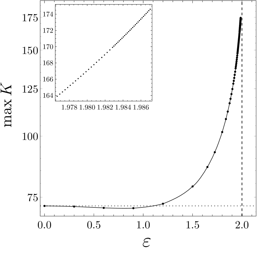
Figure 5: Log-linear plot of the curvature scalar maximum against $\varepsilon$, for a large black hole with $T=1/\pi$. The dashed gridline marks the critical value of $\varepsilon$, and the dotted gridline shows ${K_{\mathrm{max}}=72}$ for a Schwarzschild-AdS₄ black hole. The inset is a log-log plot for high values of the rotation amplitude.

In Fig. 5, we show the maximum of the Kretschmann scalar as a function of $\varepsilon$ for large black holes. For the black holes, the Kretschmann scalar is maximal on the horizon, located at $y=0$, and as $\varepsilon\rightarrow 2^{-}$, it peaks closer to $\theta=\pi/4$. For Schwarzschild-AdS₄, $L^{4}\,K|_{\mathcal{H}}=12/y_{+}^{4}+24/y_{+}^{2}+36$, and thus for $T=1/\pi$ the maximal value is $72/L^{4}$. As the boundary amplitude approaches $\varepsilon=2^{-}$, the Kretschmann scalar grows without bound (see Fig. 5) and we expect the maximum of the Kretschmann scalar to enter a scaling regime. This quantity is difficult to extract accurately, however we find some numerical evidence that it behaves as a power law as $\varepsilon\rightarrow 2^{-}$.

For completeness, we present plots of the Kretschmann scalar of the thermodynamically dominant solutions in Appendix B, Fig. 22.

4.2.3 Entropy

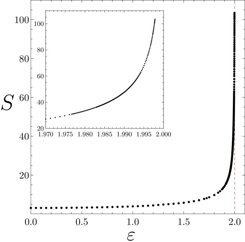
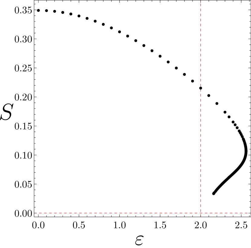
Figure 6: Left: Entropy against the rotation parameter $\varepsilon$ for the large branch of black holes with $T=1/\pi$. The inset zooms around the limit, demonstrating the asymptotic behavior. Red dashed gridlines mark the $\varepsilon=2$ limit. Middle: Logarithmic derivative of $S$ for the large black hole with $T=1/\pi$. As $\varepsilon\rightarrow 2$, the entropy of the large black hole blows up as an inverse power law. Right: Entropy of the small branch of black holes with the same temperature. Red dashed gridlines show where $\varepsilon=2$ and $S=0$.

The entropy associated with the black hole horizon is given by

$$S=\frac{A}{4G_{N}}=\frac{2\pi\,y_{+}^{2}\,L^{2}}{G_{N}}\int_{0}^{1}\mathrm{d}x\frac{1-x^{2}}{\sqrt{2-x^{2}}}\sqrt{Q_{3}(x,0)Q_{5}(x,0)}\,.$$ (13)

In Fig. 6, we present our results for the small and large branches of black hole solutions with a temperature $T=1/\pi$. For the large black holes, we find that the entropy is always an increasing function of $\varepsilon$, and as $\varepsilon\rightarrow 2^{-}$, it grows without bound. When $\varepsilon$ is sufficiently close to $2$, the entropy enters a scaling regime as we saw with the Kretschmann scalar, and $S\propto(2-\varepsilon)^{-\alpha}$ (see the middle panel of Fig. 6). Numerically we find that $\alpha$ is consistent with being $1/2$ within a $1\%$ error.

For the small branch (see right panel of Fig. 6), and fixed temperature, the entropy is a decreasing function of $\varepsilon$. In this case we can reach values $\varepsilon>2$, although we still find a maximum value of $\varepsilon$ beyond which we cannot find axially symmetric black hole solutions. We call this maximum value $\varepsilon_{\max}(T)$. As the temperature decreases, $\varepsilon_{\max}(T)$ approaches $\varepsilon_{c}$ from below, which is a turning point for the small branch of solutions, below which we obtain a second set of unstable solutions with lower entropy. In this region of the solution space numerical errors are increasingly large, and we were unable to extend the solutions by further decreasing $\varepsilon$. We conjecture that $S\rightarrow 0$ in the limit $\varepsilon\rightarrow 2^{+}$, and the singularity might be approached in a non-trivial way.

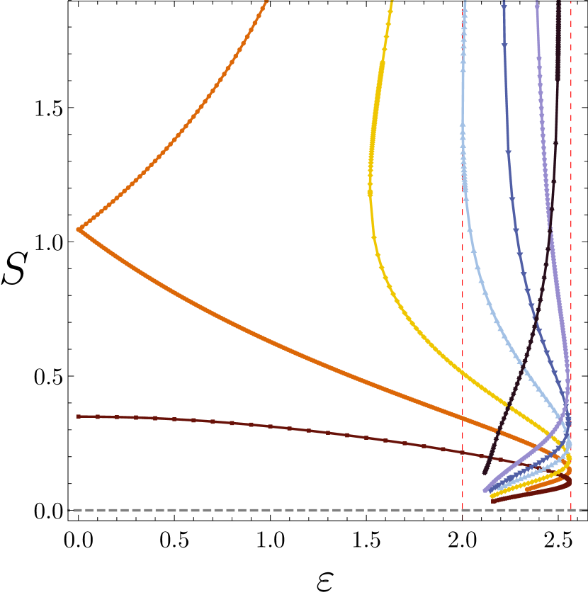
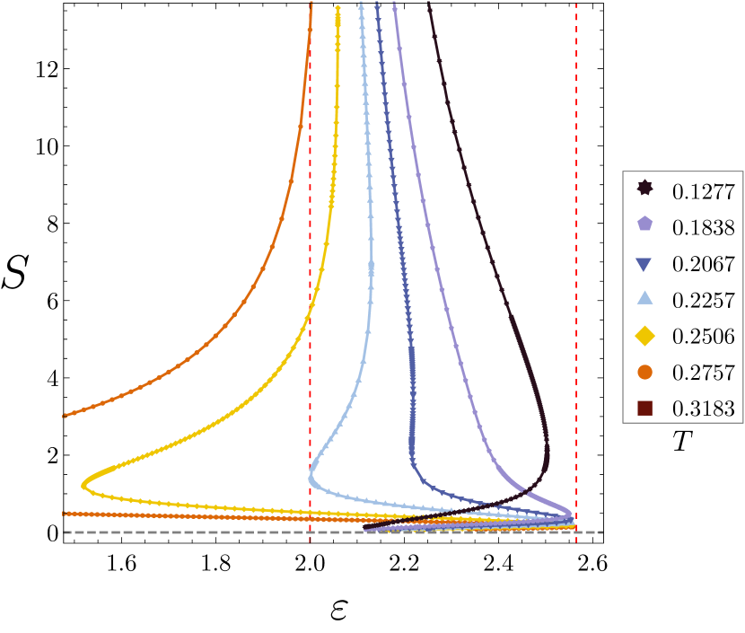
Figure 7: Left: Entropy against the boundary parameter for low temperature black holes with $T<T^{\mathrm{Schw}}_{\min}\simeq 0.2757$. The orange disks show black holes with $T\simeq T^{\mathrm{Schw}}_{\min}$. The brown squares show the (hot) small black holes with $T=1/\pi$ for reference. As we lower the temperature, the large black holes begin to exist for $\varepsilon>2$. Right: The asymptotic behavior of isothermal entropy curves. Both solution branches approach $\varepsilon=2$, with the large branch having a steeply increasing $S$, and the small branch having $S\rightarrow 0$. The red gridlines show $\varepsilon=2$ and $\varepsilon=\varepsilon_{c}$.

This picture looks qualitatively the same for black holes with $T>T^{\mathrm{Schw}}_{\min}$ (recall than $T^{\mathrm{Schw}}_{\min}\simeq 0.2757$), with large solutions expanding and small solutions shrinking down when we increase $T$. However, we can find black hole solutions with a minimal temperature $T_{\min}(\varepsilon)<T^{\mathrm{Schw}}_{\min}$. This implies that for fixed $T<T^{\mathrm{Schw}}_{\min}$, there are no black hole solutions for $\varepsilon<\varepsilon_{\min}$. As we cross the $T^{\mathrm{Schw}}_{\min}$, the two black hole branches at fixed temperature join up (see orange disks in Fig. 7), and as we lower the temperature further, the “left” turning point occurs for higher values of $\varepsilon$. The subsequent evolution of the phase space is somewhat intricate. It turns out, that for all fixed $T<T^{\mathrm{Schw}}_{\min}$, there exist large black holes with $\varepsilon>2$. There, we find yet another turning point, which bends back towards $\varepsilon=2$. For temperatures $T\lesssim 0.2257$, the “left” turning point crosses $\varepsilon=2$, and black holes exist only for $\varepsilon>2$. Soon after, once we reach $T\simeq 0.207$, the two upper turning points converge and disappear, leaving only the lower turning point, which appears to exist for all finite temperatures.

This analysis reveals interesting non-uniqueness of the black hole solutions. For temperatures ${T>T^{\mathrm{Schw}}_{\min}}$, we have two black hole solutions: for $\varepsilon<2$, there is a large and a small black hole, and for $\varepsilon>2$ there are two small black holes, if we assume that we are approaching $\varepsilon\rightarrow 2^{+}$ as $S\rightarrow 0$. For ${T<T^{\mathrm{Schw}}_{\min}}$, we have two solutions for $\varepsilon_{\mathrm{min}}(T)<\varepsilon<2$, four solutions for $\varepsilon>2$ until $T\simeq 0.2067$, when these extra phases merge, and then we again have two branches. All these solutions exist up to some value of $\varepsilon_{\mathrm{max}}(T)<\varepsilon_{c}$.

The low temperature regime is hard to access numerically, so we can only conjecture the very low temperature behaviour. The only remaining turning point is decreasing slowly with the temperature, separating the two branches of solutions the lower of which has vanishing horizon area as $\varepsilon\rightarrow 2^{+}$. These solutions look qualitatively very similar to the soliton solutions, and could be thought of as a small black hole placed in a soliton background. The upper branch has increasing entropy, which blows up as $\varepsilon\rightarrow 2^{+}$.

In the following subsections we present physical quantities and carry out an extensive thermodynamic analysis of both black holes and horizonless AdS₄ solutions, further supporting our conjectures.

4.3 Stress-Energy tensor

The bare on-shell gravity action in AdS₄ is divergent and in order to obtain the boundary stress tensor we need to regularise the action using holographic renormalization techniques Brown:1992br ; Henningson:1998gx ; Balasubramanian:1999re . The counterterms that we must add to the bulk action (1) are

$$S_{ct}=-\frac{1}{4\pi G_{N}L}\int_{\partial\mathcal{M}}\mathrm{d}^{3}x\sqrt{-\gamma}\left(1-\frac{L^{2}}{4}R[\gamma]\right),$$ (14)

and the expectation value of the stress-energy tensor of the dual field theory can be found to be

$$\langle\tilde{T}\rangle_{\mu\nu}=\frac{1}{8\pi G}\left(\Theta_{\mu\nu}-\Theta\gamma_{\mu\nu}+LG_{\mu\nu}[\gamma]-\frac{2}{L}\gamma_{\mu\nu}\right),$$ (15)

from the on-shell action.

As an exercise, following deHaro:2000vlm , we also compute the holographic stress tensor by recasting the metric (7a) into Fefferman-Graham coordinates. Firstly, we solve the equations of motion about the conformal boundary $y=1$, order by order, by expanding the metric functions as shown below

$$Q_{i}(x,y)=\sum_{n=0}^{3}(1-y)^{n}q_{i,n}(x)+\log{(1-y)}(1-y)^{4}\tau_{i,4}(x)+\mathchoice{{\scriptstyle\mathcal{O}}}{{\scriptstyle\mathcal{O}}}{{\scriptscriptstyle\mathcal{O}}}{\scalebox{0.7}{$\scriptscriptstyle\mathcal{O}$}}\left((1-y^{2})^{3}\right).$$ (16)

Next we perform an asymptotic coordinate change near the AdS₄ boundary to the Fefferman-Graham form

$$\mathrm{d}s^{2}=\frac{1}{z^{2}}\left[\mathrm{d}z^{2}+\mathrm{d}s^{2}_{\partial}+z^{2}\mathrm{d}s^{2}_{1}+z^{3}\mathrm{d}s^{2}_{2}+\mathcal{O}(z^{4})\right]\,.$$ (17)

To achieve this, we take

$$y=1+\sum_{n=1}^{4}z^{n}\,Y_{n}(\theta)+\mathchoice{{\scriptstyle\mathcal{O}}}{{\scriptstyle\mathcal{O}}}{{\scriptscriptstyle\mathcal{O}}}{\scalebox{0.7}{$\scriptscriptstyle\mathcal{O}$}}(z^{4}),$$

$$x=\sqrt{1-\sin\theta}+\sum_{n=1}^{4}z^{n}\,X_{n}(\theta)+\mathchoice{{\scriptstyle\mathcal{O}}}{{\scriptstyle\mathcal{O}}}{{\scriptscriptstyle\mathcal{O}}}{\scalebox{0.7}{$\scriptscriptstyle\mathcal{O}$}}(z^{4}),$$ (18)

and determine $\{Y_{n}(\theta),X_{n}(\theta)\}$ order by order in $z$ so that our line elements can be cast in the form (19) with conformal boundary metric

$$\mathrm{d}s^{2}_{\partial}=-\mathrm{d}t^{2}+\mathrm{d}\theta^{2}+\sin^{2}\theta\left[\mathrm{d}\phi+\mathrm{d}t\,\cos\theta\,\varepsilon\right]^{2}\,.$$ (19)

The holographic stress-energy tensor is then given by

$$\langle T_{ij}\rangle=\frac{3}{16\pi}g_{(2)ij},$$ (20)

where $g_{(2)ij}$ is the metric associated with $\mathrm{d}s_{2}^{2}$. As expected, this stress-energy tensor is traceless and transverse with respect to (19). The energy density is simply given by $\rho(\theta)=-\langle T^{t}_{\phantom{t}t}\rangle$, whilst the angular momentum density is simply $j(\theta)=\langle T^{t}_{\phantom{t}\phi}\rangle$.

4.3.1 Soliton

The independent boundary stress-energy tensor components for the soliton solution are given by

$$\langle T^{t}_{\phantom{t}t}\rangle =\frac{1}{768\pi}\left[18q_{1}(\theta)+\varepsilon\sin^{2}\theta\left\{-65\varepsilon+\sin^{2}\theta\left(3\varepsilon^{3}\sin^{2}2\theta+46\varepsilon+18q_{6}(\theta)\right)-18q_{6}(\theta)\right\}\right],$$ (21)

$$\langle T^{t}_{\phantom{t}\phi}\rangle =\frac{1}{128\pi}\sin^{2}\theta\cos\theta\left[2\varepsilon^{3}\sin^{4}\theta+3\varepsilon-3q_{6}(\theta)\right],$$ (22)

$$\langle T^{\theta}_{\phantom{\theta}\theta}\rangle =\frac{1}{768\pi}\left[\varepsilon^{2}\sin^{2}\theta(16\cos{2\theta}-27)+18q_{3}(\theta)\right].$$ (23)

Numerical results are presented in Fig. LABEL:fig:sols where we plot these components against $\theta$ for several values of the boundary rotation amplitude $\varepsilon$. The stress-energy tensor component $\langle T^{t}_{\phantom{t}t}\rangle$ is positive at the equator where it is also maximal; it becomes negative at a value which depends on $\varepsilon$, and is negative at the poles. As the rotation amplitude increases towards $\varepsilon_{c}$, $\langle T^{t}_{\phantom{t}t}\rangle$ develops a large negative minima in the upper quarter of the sphere. $\langle T^{t}_{\phantom{t}\phi}\rangle$, on the other hand, is negative for small values of $\varepsilon$, and is vanishing on both the poles and the equator. As $\varepsilon\rightarrow\varepsilon_{c}$, $\langle T^{t}_{\phantom{t}\phi}\rangle$ develops a broad, large maxima close to the equator, and for the second soliton branch, it becomes entirely positive. The component $\langle T^{\theta}_{\phantom{\theta}\theta}\rangle$, measuring the pressure along $\theta$, is positive and peaked at the equator for small values of $\varepsilon$. As the amplitude is increased, the pressure becomes very negative at the equator, increases towards the poles and develops a maxima close to $\theta=\pi/4$.

4.3.2 Black Holes

The independent holographic stress-energy tensor components for the black hole metric (7a) are given by

$$\begin{split}\langle T^{t}_{\phantom{t}t}\rangle=\frac{y_{+}}{49152\pi}\bigg{[}3y_{+}^{2}\left(635\delta^{3}-1533\delta^{2}-887\delta+384q_{1}(\theta)-263\right)-192\left(29\delta^{2}-14\delta+17\right)\\ +16\varepsilon\sin^{2}{\theta}\left\{\sin^{2}{\theta}\left(-12\varepsilon^{3}\cos{4\theta}+72q_{6}(\theta)y_{+}^{2}+\varepsilon\left(-1113\delta+12\varepsilon^{2}-288y_{+}^{2}+2285\right)\right)\right.\\ \left.-72q_{6}(\theta)y_{+}^{2}+32\varepsilon\left(27\delta+9y_{+}^{2}-65\right)\right\}\bigg{]},\\ \end{split}$$ (24)

$$\langle T^{t}_{\phantom{t}\phi}\rangle =\frac{y_{+}}{128\pi}\sin^{2}{\theta}\cos{\theta}\left[4\varepsilon^{3}\sin^{4}{\theta}-3q_{6}(\theta)y_{+}^{2}+12\varepsilon\left(3\delta+y_{+}^{2}-5\right)\right],$$ (25)

$$\begin{split}\langle T^{\theta}_{\phantom{\theta}\theta}\rangle=\frac{y_{+}}{49152\pi}\left[192\left(7\delta^{2}+26\delta-17\right)+3y_{+}^{2}\left(-109\delta^{3}+315\delta^{2}+721\delta+384q_{3}(\theta)+97\right)-\right.\\ \left.16(33\delta+139)\varepsilon^{2}\sin^{4}{\theta}-1024\varepsilon^{2}\sin^{2}{\theta}\right].\end{split}$$ (26)

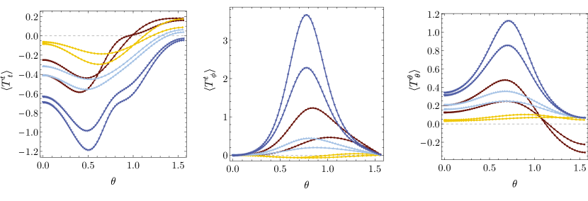
Figure 24: Boundary energy-stress tensor components for a fixed low temperature (${T=0.2506}$), where there are four possible black hole phases: lowest entropy black hole branch (brown squares), small black hole branch (yellow diamonds), thermodynamically dominant middle branch (faint blue triangles) and largest entropy large black holes (blue upside-down triangles).

Numerical results for several values of the black hole temperature and boundary rotation amplitude are presented in Fig. LABEL:fig:bhtensor (and for low temperatures see Appendix B, Fig. 24). For small $\varepsilon$ and large $T$, $\langle T^{t}_{\phantom{t}t}\rangle$ is entirely negative. It is maximal at the equator and minimal at a value which depends on both $\varepsilon$ and $T$, where it also attains its largest absolute value. If we fix $T$ and increase $\varepsilon$, the energy density at the equator decreases, and becomes slightly negative. As expected, for a fixed boundary amplitude, the energy density is an increasing function of temperature.

The component $\langle T^{t}_{\phantom{t}\phi}\rangle$ is negative for small $\varepsilon$ and temperatures close to $T_{\mathrm{min}}(\varepsilon)$, and vanishes at the poles and at the equator, similarly to the soliton case. Generally, $\langle T^{t}_{\phantom{t}\phi}\rangle$ is a complicated function of $T$ and $\varepsilon$. For a fixed value of $\varepsilon$, it is an increasing function of temperature, and for large enough temperatures it becomes large and entirely positive. In particular, when $\varepsilon\rightarrow 2$, the density develops a large positive maxima peaked at $\theta=\pi/4$.

The anisotropic pressures capture some qualitative behaviour of the system. The normal stress component along $\theta$ is positive for all $\varepsilon$ and $T$, and for a fixed rotation amplitude is an increasing function of temperature. Furthermore, for a fixed temperature, it is an increasing function of $\varepsilon$. In the large temperature, large $\varepsilon$ regime, $\langle T^{\theta}_{\phantom{\theta}\theta}\rangle$ develops a broad positive maxima, peaked in the vicinity of $\theta=\pi/4$. The normal stress component in the direction of $\phi$ (not pictured) can be negative around the equator, and in the large $\varepsilon$, $T$ regime, it is positive with a sharp dip to negative values at $\theta=\pi/4$.

4.4 Thermodynamics

4.4.1 Energy

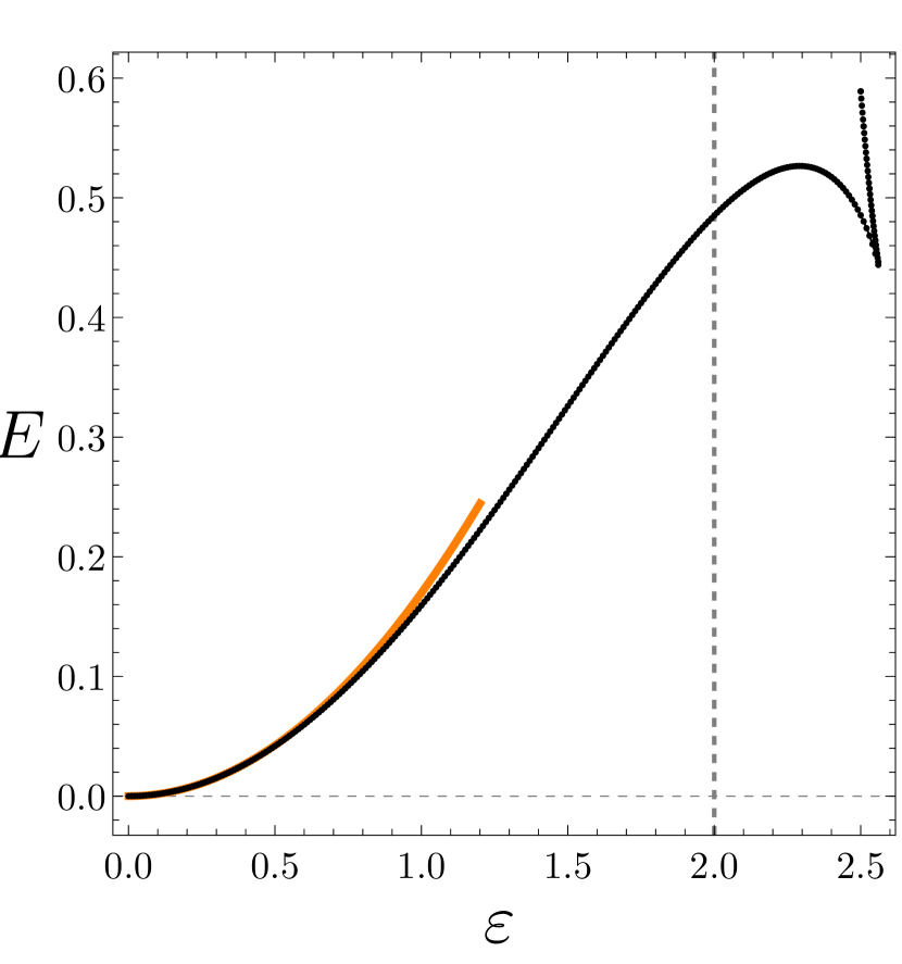
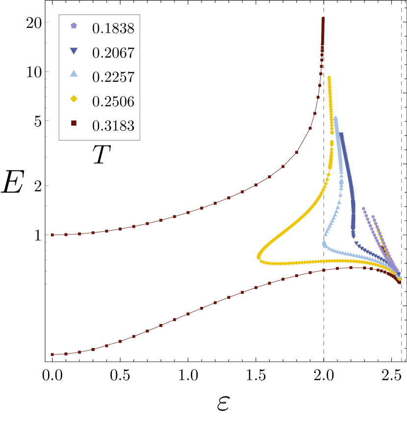
Figure 10: Left: Soliton solution boundary energy against rotation parameter. The dashed vertical gridline marks the critical amplitude $\varepsilon=2$, and the bold orange line is the perturbative result. Right: Log-linear plot of the energy for the black hole solutions against $\varepsilon$, for several values of $T$.

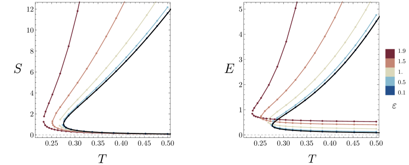
Figure 11: Left: Black hole entropy against temperature for several values of the boundary rotation parameter $\varepsilon$, for $\varepsilon<2$. The upper branches correspond to the large solutions and the lower branches to the small solutions. Right: Black hole energy as a function of temperature. Colouring codes the value of the boundary amplitude. The bold black curve is the Schwarzschild-AdS₄ solution with $\varepsilon=0$.

We obtain conserved charges in the usual way by integrating the angular momentum and energy densities Brown:1992br . We note that by construction, $\varepsilon=0$ solutions take the Schwarzschild-AdS₄ values, $T=(1+3y_{+}^{2})/(4\pi y_{+})$, $S=\pi y_{+}^{2}$, $M=y_{+}(1+y_{+}^{2})/2$ and $G=y_{+}(1-y_{+}^{2})/4$, discussed below.

As expected, the total angular momentum is identically zero. We present the energy for black holes as a function of $\varepsilon$ and $T$ on the right panels of Fig. 10 and Fig. 11, respectively. For a fixed $\varepsilon$ and varying $T$, the large black holes increase their energy, and the small black holes decrease it, asymptotically approaching $E\rightarrow 0$. Further, for a fixed $T$ and increasing $\varepsilon$, the large black hole energy increases monotonically, as does the small black hole energy for $\varepsilon<2$, which is the opposite behaviour to that of the entropy (see left panel of Fig. 11).

For values $2<\varepsilon<\varepsilon_{\mathrm{max}}(T)$, where $\mathrm{max}(T)$ was identified in the discussion of Fig. 6 and Fig. 7, the solution space has extra phases associated with cold temperatures. As we lower the temperature, the black hole energy approaches $\varepsilon=2$ from above, but unlike entropy, it appears to blow up for both small and large solution branches. As we lower $T$ further, black holes eventually exist only for $\varepsilon>2$, and the two branches appear to have similar values of energy.

The holographic energy for the soliton is presented on the left panel of Fig. 10. With increasing boundary parameter $\varepsilon$, the energy is increasing until it peaks at $\varepsilon\simeq 2.29$ with maximum energy $E_{\mathrm{max}}\simeq 0.527$ for the small branch. The large branch has larger energy, which increases steeply when $\varepsilon\rightarrow 2^{+}$. We constructed these solutions numerically up to $\varepsilon=2.3$, however numerical errors in this region of the parameter space become increasingly large.

4.4.2 Grand-canonical ensemble

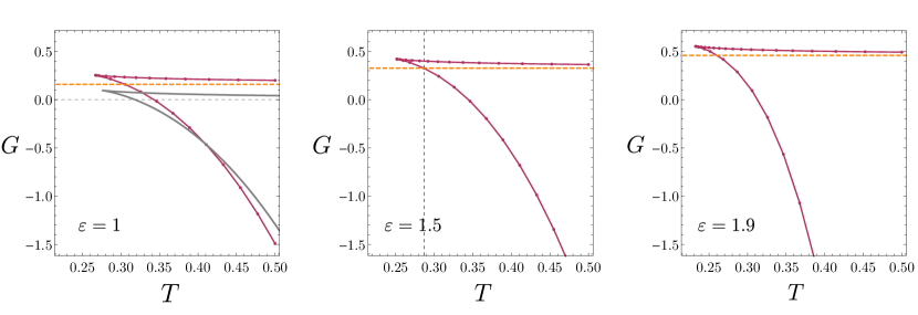
Figure 12: Left: Gibbs free energy for the black holes against temperature for a fixed boundary rotation parameter $\varepsilon=1$ (red data points). The orange gridline shows the value for the corresponding AdS₄ soliton with the same $\varepsilon$. The grey solid curve traces the values of Schwarzschild-AdS₄, and the grey-dashed gridline shows $G_{\mathrm{AdS}}=0$. Middle: Similar plot for $\varepsilon=1.5$, with the horizontal gridline marking the intersection temperature $T_{\mathrm{HP}}(\varepsilon)$. To the right of this line the large black holes will be the dominant solutions, whilst solitons dominate to the left. Right: As we approach the critical value of $\varepsilon$, the phase transition temperature decreases.

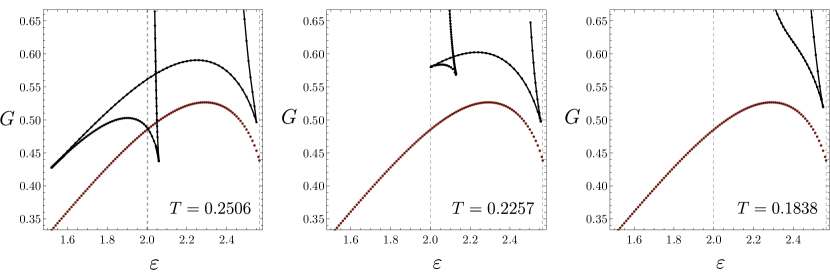
Figure 13: Gibbs free energy against the boundary parameter for low temepreature black holes. It exhibits a swallowtail phase transition between the inelastic black hole phase and the soliton (brown stars).

Because we can fix the boundary chemical potential and temperature $T$, the appropriate thermodynamic ensemble for analysing our solutions is the grand-canonical ensemble. In this ensemble the preferred phase minimises the Gibbs free energy

$$G=E-TS\,.$$ (27)

Note that in this system the energy, $E$, absorbs the chemical potential term, and in particular for solitons we have $G=E$. This is further supported by the first law of thermodynamics for these solutions, derived following Iyer:1994ys ; Papadimitriou:2005ii ; Compere:2007vx , and given by

$$\mathrm{d}E=T\,\mathrm{d}S+4\pi\int_{0}^{\pi/2}\mathrm{d}\Omega(\theta)j(\theta)\,\sin\theta\,\mathrm{d}\theta,$$ (28)

where $\Omega(\theta)=\varepsilon\cos\theta$ is the boundary angular velocity density, and $j(\theta)$ is the angular momentum density. In order to check the first law we constructed soliton solutions perturbatively to second order, the procedure for which is detailed in Appendix C. We use the second order expansion to calculate the boundary free energy to be $E=8\varepsilon^{2}/(15\pi)$, which matches our numerical solutions to small $\varepsilon$ amplitude (see left panel of Fig. 10) and satisfies the first law (28) to first order in $\varepsilon$. Numerically, the first law is satisfied to at least to $0.1\%$ for the small soliton branch, to $2\%$ for the large branch, and to $0.1\%$ for the black holes (with $2\%$ for the second set of the small black holes), while varying $\varepsilon$. For black holes it is also satisfied to $0.1\%$, while varying temperature and keeping the boundary profile fixed.

We next discuss our results in terms of free energy. In Fig. 12, we present $G$ for the black hole solutions as a function of the temperature for some values of the rotation amplitude. For a fixed $\varepsilon$, the corresponding soliton energy (see Fig. 10) is constant, which is pictured as a line. The intersection of the two marks the generalised Hawking-Page transition Hawking:1982dh , and the transition temperature $T_{\mathrm{HP}}(\varepsilon)$ is a decreasing function of $\varepsilon$. For temperatures higher than the transition value, the large black hole phase is the dominant one, whilst for ${T<T_{\mathrm{HP}}(\varepsilon)}$ the soliton is the preferred phase.

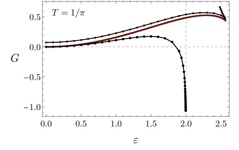
Figure 23: Left: Gibbs free energy against the boundary profile for black holes with a fixed temperature $T=1/\pi$ (black disks), and soliton (brown squares). The dashed gridline marks the $\varepsilon\rightarrow 2$ limit. Right: Maximum of the Kretschmann invariant against $\varepsilon$ for the small black hole with a fixed temperature. As $\mathrm{max}\,K$ increases, the $K$ looks very similar to that of the soliton.

For $T<T^{\mathrm{Schw}}_{\mathrm{HP}}=1/\pi$, we observe curious phase transitions in $G$, characterised by a “swallowtail” behaviour in the Gibbs free energy Chamblin:1999tk ; Chamblin:1999hg (Fig. 13). This occurs because large black holes start to exist past $\varepsilon=2$, where there is a turning point in the parameter space resulting in a four-fold non-uniqueness, and thus there exists a moduli space for which we have four possible black hole phases (and two soliton phases). We find that for $0.24<T<1/\pi$, there is a temperature dependent interval $\varepsilon_{\mathrm{HP}}(T)<\varepsilon<\varepsilon_{\mathrm{\star}}(T)$ with $\varepsilon_{\mathrm{\star}}(T)>2$, where the cold, inelastic black holes dominate the ensemble. Finally, we note that the small black hole branch is never favoured thermodynamically, as it always has higher free energy than both the large black hole and the soliton. The corresponding phase diagram is illustrated in Fig. 14. We also present $G$ as a function of $\varepsilon$ for a fixed temperature in Appendix B (see the left panel of Fig. 23).

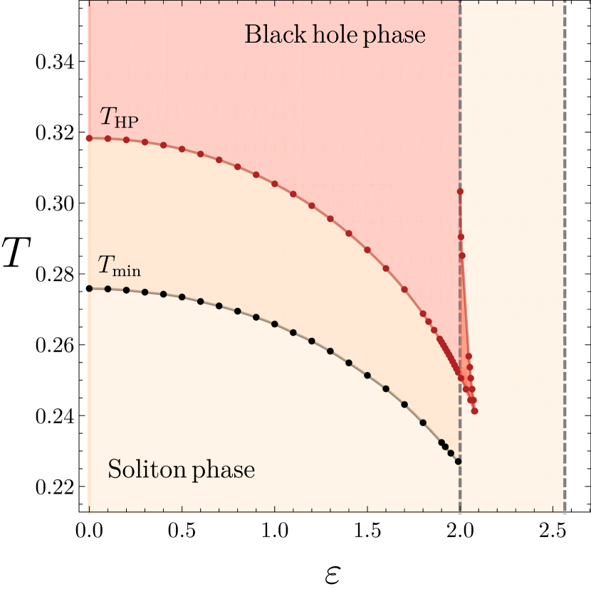
Figure 14: Phase diagram for the rotationally polarised solutions. For $\varepsilon<2$, black holes exist above $T_{\mathrm{min}}(\varepsilon)$ (black data points) and are the dominant phase above the $T_{\mathrm{HP}}(\varepsilon)$ curve (red area) which marks the corresponding Hawking-Page transition. Below the transition line (red data points), the dominant phase is the soliton. For $\varepsilon>2$, there is a cold inelastic black hole phase (red wedge). The elsewhere subdominant black holes exist up to some maximum $\varepsilon_{\mathrm{max}}(T)$, but are hidden by the soliton phase.

5 Stability

5.1 Quasinormal modes

To investigate the stability, we consider a wave equation for a neutral, minimally coupled scalar field

$$\Box\Phi=0\,.$$ (29)

Since both solitons and black holes have two commuting Killing fields, $\partial_{t}$ and $\partial_{\phi}$, we can decompose the perturbations as follows

$$\Phi=\widehat{\Phi}_{\omega,m}(x,y)e^{-i\,\omega\,t+i\,m\,\phi}\,.$$

The resulting equation for $\widehat{\Phi}_{\omega,m}$ is linear and can be regarded as a Sturm-Liouville problem for the eigenpair $\{\widehat{\Phi}_{\omega,m},\omega\}$, once suitable boundary conditions are imposed. The set of all $\omega$ are called the quasinormal mode (QNM) frequencies. For each value of $m$, there is an infinite number of QNM frequencies labelled by two integers. These are in one to one correspondence with the number of nodes along the $x$ and $y$ directions. If $\varepsilon=0$, we can use the background spherical symmetry to decompose the angular part in terms of spherical harmonics. These are labeled by $\ell$ and $m$, with $\ell-|m|$ counting the number of nodes along the polar angular direction. We will be interested in following the modes with $\ell=|m|$ as a function of $\varepsilon$, that is to say, modes with no nodes along the polar direction. Furthermore, we will also be focusing on the modes which have no nodes along the radial direction, i.e. with zero overtone. We focus on these modes since they have the largest $|\mathrm{Im}(\omega)|$ for fixed $m$.

We follow the method of Cardoso:2013pza ; Dias:2013sdc ; 2016CQGra..33m3001D and solve the resulting eigenvalue equation system using a Newton-Raphson method, on a fixed numerical solution background with a corresponding numerical grid.

The QNM spectrum with $\varepsilon=0$ is well–known: the Schwarzschild AdS₄ black hole QNM frequencies are given in Horowitz:1999jd , and the scalar normal mode frequencies of AdS₄ are given by integers $L\,\omega=3+\ell$. As we vary the boundary rotation parameter, the imaginary part of the black hole frequency $\omega$ becomes positive, indicating the presence of an instability.

The boundary conditions imposed at $y=0$ will depend strongly on the background solution we wish to perturb.

5.1.1 Soliton

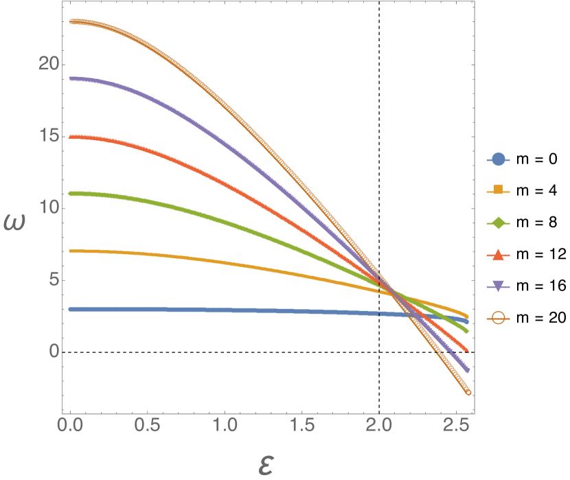
Figure 15: Left: Normal mode frequencies with $\ell=m$ vs the boundary rotation parameter $\varepsilon$ for the soliton metric. At $\varepsilon=0$ these reduce to the usual AdS₄ frequencies $L\,\omega=3+\ell$. Dashed gridlines show where $\varepsilon=2$ and $\mathrm{Re}\,\omega=0$. Right: Rotation amplitude $\varepsilon_{\times}$, where $\omega^{2}$ becomes negative, against $m$. The inset shows the logarithmic derivative of $\varepsilon_{\times}$. We expect that in the limit $m\rightarrow\infty$, $\varepsilon_{\times}\rightarrow 2$.

We first investigate scalar perturbations (29) on soliton backgrounds, and consider the following decomposition

$$\Phi(t,x,y,\phi)=e^{-i\omega t}e^{im\phi}y^{|m|}(1-y^{2})^{3}(1-x^{2})^{|m|}\psi(x,y),$$ (30)

where the factorisation ensures regularity at the origin for a smooth function $\psi(x,y)$. The boundary conditions at $y=1$ and $x=1$ are obtained by solving the equation (29) at the corresponding boundaries and are given by

$$|m|\,\psi(x,y)+\partial_{y}\psi(x,y)=0\quad\text{at}\quad y=1\,,$$ (31a)

and

$$\partial_{x}\psi(x,y)=0\quad\text{at}\quad x=1\,.$$ (31b)

We also require $\partial_{x}\psi(x,y)=0$ at $x=-1$ and $\partial_{y}\psi(x,y)=0$ at $y=0$.

On the left panel of Fig. 15, we plot the normal mode frequencies $\omega$ with $\ell=m$, against $\varepsilon$. The $\omega$ first becomes negative when $m=13$, and with each subsequent mode, $\omega$ becomes negative at a lower value of $\varepsilon$. We denote the value at which $\omega$ changes sign by $\varepsilon_{\times}$, and we find that $\varepsilon_{\times}-2\sim 1/m$ at large $m$ (see right panel of Fig. 15).

In order to better resolve where $\omega$ becomes negative for a given $m$, we can also set $\omega=0$ and look for zero–modes directly, and the results for this approach are presented in Fig. 15, right. We find that this method gives us the same values of $\varepsilon_{\times}$ as the ones inferred from computing $\omega$ directly. For each pair of values of $\{m,\varepsilon_{\times}\}$, we expect a given hairy family with nontrivial $\Phi$ to condensate. Whether this new family of hairy solutions will extend to large or small values of $\varepsilon$, is likely to depend on the model. We have constructed soliton solutions with complex scalar hair within cohomogeneity two, and will present these solutions elsewhere. These were built by minimally coupling a massless complex scalar field to gravity, and are similar in spirit to the black holes with a single Killing field of Dias:2011at and to the holographic Q-lattices of Donos:2013eha .

5.1.2 Black hole

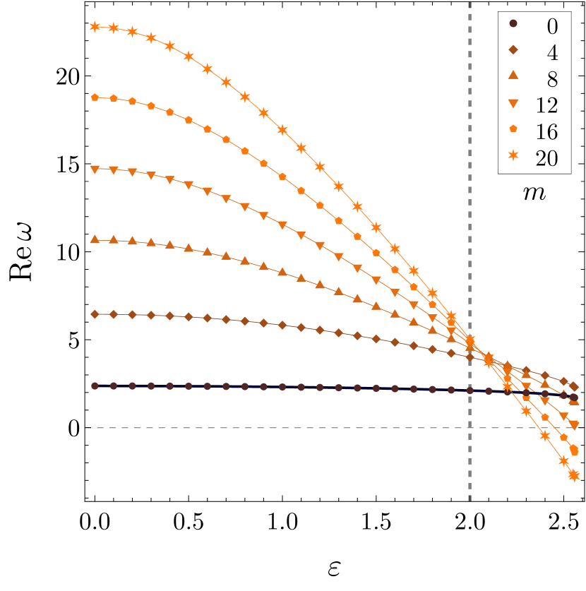
Figure 16: Left: Real part of quasinormal mode frequency with $\ell=m$ against the boundary rotation parameter $\varepsilon$, for small black holes with $T=1/\pi$. At $\varepsilon=0$, these reduce to the Schwarzschild-AdS₄ values. The bold dashed gridline shows the critical $\varepsilon=2$ value. Right: Rotation amplitude where the zero–mode is for a given $m$, against $m$. The inset shows the logarithmic derivative of $\varepsilon_{\times}$. We expect that in the limit $m\rightarrow\infty$, $\varepsilon_{\times}\rightarrow 2$.

Next, we consider the black hole solutions. A Frobenius analysis at the integration boundaries motivates the following separation ansatz

$$\Phi(t,x,y,\phi)=e^{-i\omega t}e^{im\phi}y^{-i\frac{2\omega y_{+}}{1+3y_{+}^{2}}}(1-y^{2})^{3}(1-x^{2})^{|m|}\psi(x,y)\,,$$ (32)

where we have implicitly imposed regularity in ingoing Eddington-Finkelstein coordinates Horowitz:1999jd .

The boundary conditions for $\psi(x,y)$ at $y=1$ and $x=1$ are then found by solving (29) and demanding that $\psi(x,y)$ has a regular Taylor expansion at $y=1$ and $x=1$. This in turn gives:

$$-2i\,y_{+}\omega\psi(x,y)+(1+3y_{+}^{2})\partial_{y}\psi(x,y)=0\quad\text{at}\quad y=1\,,$$ (33a)

and

$$\partial_{x}\psi(x,y)=0\quad\text{at}\quad x=1\,.$$ (33b)

As with the soliton, we require $\partial_{x}\psi(x,y)=0$ at $x=-1$ and $\partial_{y}\psi(x,y)=0$ at $y=0$.

Numerical results are presented in Fig. 16. On the left panel, we plot the real part of the QNM frequencies with $\ell=m$ against $\varepsilon$, for a fixed $T=1/\pi$ small black hole branch. We find that the behaviour of $\mathrm{Re}\,\omega$ is very similar to that of the soliton, and the first unstable mode appears at $m=13$. The imaginary part, $\mathrm{Im}\,\omega$, becomes positive exactly where $\mathrm{Re}\,\omega$ crosses the zero axis, indicating a zero–mode. If we set $\omega=0$ and look for these directly, we again find a $1/m$ fall–off (see right panel of Fig. 16) at large $m$. The growth rate of the instability is less than $\Gamma\sim 10^{-20}$, so it sets in incredibly slowly. We expect that these solutions will become unstable in modes with high $m$ as we increase the boundary rotation past $\varepsilon=2$ and, if we assume the $1/m$ decay, the instability should manifest itself slowly with increasing $\varepsilon$. Finally, for hot, large black holes we do not see any sign of instability, as these solutions never cross $\varepsilon=2$.

This is a surprising result - the ergoregion appears to induce hairy solutions in both phases. This opens up new possibilities for the phase diagram, some of which we will discuss in the following sections. This section was devoted entirely to the stability analysis of scalar perturbations, and the issue of the stability of our backgrounds with respect to gravitational perturbations is an open problem. However, if we assume that the physics involved in this instability is any similar to the usual superradiance instability, we expect the gravitational perturbations to be unstable and to have larger instability growth rates.

6 Field Theory

Our calculation in this section follows mutatis mutandis that of Section 4.1 of Costa:2015gol . We will first consider a conformally coupled scalar field satisfying the Klein-Gordon equation on $\mathbb{R}_{t}\times S^{2}$. The idea is to determine the eigenfunctions on this background, and use those to determine the spectrum of a conformally coupled scalar on the rotating background (2).

If $\varepsilon=0$, the Klein-Gordon equation for a conformally coupled scalar in $1+2$ reads (where we set the radius of the $S^{2}$ to unity):

$$-\frac{\partial^{2}}{\partial t^{2}}\varphi+\nabla^{2}_{S^{2}}\varphi=\frac{1}{4}\varphi\,.$$

The Hamiltonian eigenstates are given by spherical harmonics $|\ell,m\rangle$, with wave-functions

$$\langle\theta,\phi|\ell,m\rangle=Y_{\ell m}(\theta,\phi)\,.$$

In this basis, the Hamiltonian $\hat{H}=i\partial/\partial t$ has the following spectrum

$$\hat{H}|\ell,m\rangle=\left(\ell+\frac{1}{2}\right)|\ell,m\rangle\,.$$

After turning on the electric field, the Hamiltonian is deformed into

$$H=\sqrt{\frac{1}{4}-\nabla_{S^{2}}+\frac{\varepsilon^{2}}{16}\sin^{4}\theta}+i\,\varepsilon\,\cos\theta\,\frac{\partial}{\partial\phi}\,.$$

Since $H$ commutes with $\partial/\partial\phi$, it will remain diagonal in the azimuthal quantum number $m$. However, it is no longer diagonal in $\ell$, and its elements have to be computed numerically:

$$\langle\ell^{\prime}m^{\prime}|H|\ell m\rangle=\delta_{m,m^{\prime}}\Bigg{\{}\int_{0}^{2\pi}\mathrm{d}\,\varphi\int_{0}^{\pi}\mathrm{d}\theta\,\sin\theta\,\bar{Y}_{\ell^{\prime}m}\,\sqrt{\ell\left(\ell+\frac{1}{2}\right)+\frac{\varepsilon^{2}}{16}\sin^{4}\theta}\,Y_{\ell m}\\ -m\,\varepsilon\,\left[\delta_{\ell,\ell^{\prime}-1}\sqrt{\frac{(\ell+1+m)(\ell+1-m)}{(2\ell+1)(2\ell+3)}}+(\ell\leftrightarrow\ell^{\prime})\right]\Bigg{\}}.$$ (34)

For each value of $m$, we can truncate the values of $\ell$ and $\ell^{\prime}$ up to some maximum value $\ell_{\max}$ and determine the eigenvalues numerically. One can show that if we are only interested in a few low lying modes, the convergence is exponential in $\ell_{\max}$. The results are illustrated in Fig. 17 where we plot the lowest lying eigenvalue of $\langle\ell^{\prime}m|H|\ell m\rangle$, which we denote by $\lambda_{m,0}$, for several values of $m=2,6,10,14$. The similarity between the left panel of Fig. 15 and the left panel of Fig. 17 is striking.

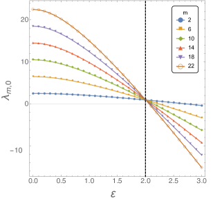
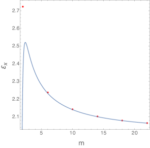
Figure 17: Left: Lowest lying mode eigenvalue of the boundary hamiltonian as a function of the boundary rotation parameter $\varepsilon$. At $\varepsilon=0$ these reduce to $\ell+1/2$. Right: $\varepsilon$ above which $\lambda_{m,0}$ becomes negative, plotted as a function of $m$. The solid line represents our analytic approximation (35) valid at large $m$.

One can go further and compute the critical value of $\varepsilon$ above which $\lambda_{m,0}$ becomes negative, and compare it with the right panel of Fig. 15. We call this special value $\varepsilon$ $\varepsilon_{\times}$, in accordance to section 5. In the large $m$ limit, the Hamiltonian can be diagonalised using a WKB approximation, and can be used to determine $\varepsilon_{\times}$. We have performed this calculation to order $m^{-12}$, and it turns out that

$$\varepsilon_{\times}=2+\frac{\sqrt{2}}{m}-\frac{3}{32m^{2}}+\frac{1}{32\sqrt{2}m^{3}}-\frac{85}{2048m^{4}}-\frac{5427}{32768\sqrt{2}m^{5}}-\frac{132879}{524288m^{6}}-\frac{8720967}{8388608\sqrt{2}m^{7}}\\ -\frac{322048277}{134217728m^{8}}-\frac{109314890677}{8589934592\sqrt{2}m^{9}}-\frac{5202962510427}{137438953472m^{10}}-\frac{550282627773161}{2199023255552\sqrt{2}m^{11}}\\ -\frac{32005862571264331}{35184372088832m^{12}}+\mathcal{O}(m^{-13})\,.$$ (35)

The validity of this approximation is tested on the right panel of Fig. 17, where we can see that for $m\geq 10$, the error is below $0.1\%$ and for $m\geq 22$ it is below $0.02\%$.

7 Equilibrium of spinning test particles

The spacetimes we consider are stationary, however, the black hole solution has zero angular velocity on the horizon, and vanishing total angular momentum. If we place a small Kerr hole on the axis of symmetry, there will be a general relativistic “spin–spin” force acting on the spinning black hole, which for stationary fields can be thought of as analogous to the electromagnetic “dipole–dipole” force with opposite sign PhysRevD.6.406 ; Natario:2007pu ; PhysRevD.93.104006 . In this section, we will investigate whether it is possible to have a spinning test particle hovering above the central black hole, balanced by the pull towards the black hole and the “spin–spin” interaction with the boundary.

Equilibria of spinning test particles can be studied using the Mathisson-Papapetrou (MP) equations Mathisson2010 ; Papapetrou248 ; Pirani:1956tn ; 592311013 ; doi10.1063/1.1704055 ; Dixon1964 ; Dixon499 (for a review see 1999MNRAS.308..863S ), which are derived by taking a multipole expansion about a suitably defined reference worldline. Truncated at dipole order, they are given by

$$\begin{split}\frac{Dp^{\mu}}{Ds}&=-\frac{1}{2}R^{\mu}_{\nu\rho\sigma}v^{\nu}S^{\rho\sigma},\\ \frac{DS^{\mu\nu}}{Ds}&=p^{\mu}v^{\nu}-p^{\nu}v^{\nu},\end{split}$$ (36)

where $p^{\mu}$ is the four-momentum of the particle, which in general is not co-linear with the kinematic four-velocity $v^{\mu}$. They are related by $p^{\mu}=mu^{\mu}-u_{\nu}\dot{S}^{\mu\nu}$, where $S^{\mu\nu}$ is the anti-symmetric spin matrix and $m$ is a mass parameter. We also require a supplementary spin condition to fix the center of mass, which we choose to be the Tulczyjew-Dixon condition $p_{\nu}S^{\mu\nu}=0$. On the rotation axis, it is equivalent to the Mathisson-Pirani condition.

We will be concerned with the static case, thus setting $\dot{S}^{\mu\nu}=0$ and $\dot{p}^{\mu}=0$. This implies $m=M$ and $p^{\mu}=Mu^{\mu}$, where $M$ is the rest mass of the particle $-M^{2}=p_{\mu}p^{\mu}$. Together with the spin magnitude, defined as $S^{2}=S_{\mu\nu}S^{\mu\nu}/2$, these are constant throughout the motion. These conditions, in conjunction with the MP equations (36), are sufficient to determine the static ratio $S/M$ as a function of the radial coordinate. Equivalently, we can instead consider a conserved quantity which includes the spin potential energy

$$E=-p^{\rho}\xi_{\rho}+\frac{1}{2}\xi_{\rho;\sigma}S^{\rho\sigma},$$ (37)

where $\xi=\partial_{t}$ is the time Killing vector field, and $E>0$ is the energy at infinity of a spinning particle. The first term is conserved for a non-spinning particle, and is positive when the Killing vector is future directed and timelike. Using the normalization $-M^{2}=p_{\mu}p^{\mu}$, we can find an effective potential for radial on-axis motion of a spinning particle. In order to find equilibrium points, we look for local minima of the potential $\dot{r}^{2}+V(r)=0$, which constrains both the energy $E$, and the ratio $S/M$.

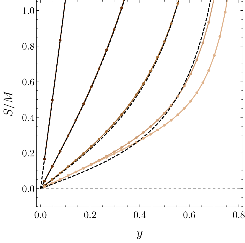
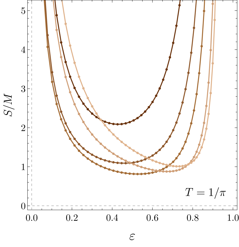
Figure 18: Left: Spin to mass ratio for a spinning test particle in the soliton background with boundary parameter $\varepsilon=0.1,0.4,1,2,2.5$ (corresponding colours vary from dark to light). Dashed black lines show analytic perturbative approximations (50) (pictured for $\varepsilon\leq 2$) which, for small $\varepsilon$, are in a very good agreement with numerical solutions. Right: Spin to mass ratio for large black holes with $T=1/\pi$, for $\varepsilon=0.1,0.5,1,1.5,1.93,1.99$ (corresponding colours vary from dark to light).

We calculate these quantities for the black hole metric (7a) and the soliton metric (5). Because our coordinates are not well-defined on the symmetry axis $\theta=0$, we first perform a local coordinate change

$$\begin{split}1-x^{2}=x_{1}^{2}+x_{2}^{2},\qquad\qquad\tan{\phi}=x_{2}/x_{1},\end{split}$$ (38)

and the symmetry axis is now given by $x_{1}=0$ and $x_{2}=0$. The supplementary condition implies that the only non-vanishing component of the spin matrix is $S^{x_{1}x_{2}}$, making the on-axis calculation considerably easier. The effective potential is then found to be

$$\begin{split}&V(r)=(g_{rr}g_{tt})^{-1}\left[g_{tt}+\left(\frac{E}{M}+\frac{S}{M}y^{\alpha}Q_{6}(1,y)\right)^{2}\right],\end{split}$$ (39)

where $\alpha=1$ for the soliton, and $\alpha=2$ for the black hole. The spin potential energy term depends on the metric ansatz, and in the expression (39) it is evaluated explicitly. The total energy of a spinning particle is

$$\frac{E}{M}=\sqrt{-g_{tt}}-\frac{S}{M}y^{\alpha}Q_{6}(1,y),$$ (40)

and the spin to mass ratio of a static spinning test particle on the symmetry axis is

$$\frac{S}{M}=\frac{-\partial_{y}g_{tt}(1,y)}{2y^{\alpha-1}\sqrt{-g_{tt}(1,y)}(2^{\alpha-1}Q_{6}(1,y)+y\partial_{y}Q_{6}(1,y))}.$$ (41)

Numerical results for both solutions are presented in Fig. 18. For the test body approximation, the Møller radius describing the minimum size of a rotating body is $R\geq S/M$ 587743163 , and it should be possible to make it arbitrarily small PhysRevD.6.406 . For the black holes, we do not find such a limiting process. For the soliton, this quantity vanishes as $y\rightarrow 0$, thus it is possible to place a spinning particle at this point, whose backreaction would lead to the formation of a small Kerr-AdS₄ black hole.

7.1 Equilibrium for non-spinning test particles

For static spacetimes the equilibrium positions are independent of spin, and can be achieved by balancing electromagnetic and gravitational forces, or coincide with the static radius due to a repulsive cosmological constant $\Lambda>0$. For Kerr black holes carter1968 , it is well known that no equilibrium positions exist PhysRevD.6.406 . Generally, conditions for equilibrium on the rotation axis are independent of the spin of the test particle. From (41), we can see that the requirement $S/M\rightarrow 0$ implies that the equilibrium conditions coincide with the minima of the static potential $-g_{tt}$.

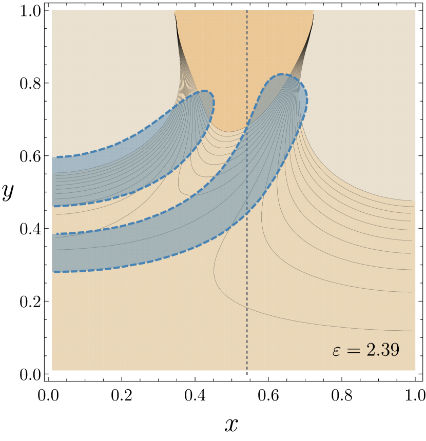
Figure 19: Left: Minima of static potential, $-g_{tt}$, for the soliton against the boundary parameter. For $\varepsilon<2$, there is a global minima at $y=0$. For ${\varepsilon>2}$, the minima is only local, owing to the fact that there is an ergoregion attached to the boundary. For the second branch, the local minima is on the $x=0$ axis, and for $\varepsilon\gtrsim 2.43$, the minima is no longer local. Right: Contour plot for $-g_{tt}$ for the second branch soliton, at $\varepsilon=2.39$. Black lines mark the contours, with the orange area around $\theta=\pi/4$ (black dashed gridline) showing the ergoregion, and the fainter orange being the positive areas, where the function increases rapidly. Overplotted in blue are the zero contours of the Kretchmann scalar, $K$, whilst the shaded areas are the two minima with a steep maxima between them.

The evolution of $-g_{tt}$ with the boundary parameter is non-trivial, and is related to the changes in the Kretchmann scalar $K$. For the soliton with $\varepsilon<2$, there is a global minima at $y=0$ (see the left panel of Fig. 19, and c.f. 2017JHEP…06..024C , Fig. 6). When $\varepsilon\geq 2$, $-g_{tt}$ becomes very negative near the boundary due to the ergoregion, and the central minima is then local. For the second branch, the minima moves up the equator towards the boundary, and as $\varepsilon\rightarrow 2$, the minima is found closer to where $K$ has the largest gradient. The ergosurface becomes visibly deformed towards the $x=0$ boundary, and the local minima eventually connects to the ergoregion at $\varepsilon\gtrsim 2.43$ (see the right panel of Fig. 19).

For the large hot black hole solutions, the minima of $-g_{tt}$ is on the horizon, tending to $\theta=\pi/4$ as $\varepsilon\rightarrow 2$. The corresponding small branch has a turning point at $\varepsilon>2$, where the entropy $S\rightarrow 0$ (see the right panel of Fig. 6). The small black holes, for all temperatures, are similar to soliton solutions. When the black hole entropy is small, $-g_{tt}$ looks very similar to the soliton (see the right panel of Fig. 19), but with the local minimum along the horizon.

Finally, we comment on the stability of the test particles. For the stable soliton branch ($\varepsilon>2$), the (spinning) particles can be put at the global minimum of the static potential, however, such solutions are not thermodynamically favoured. Let us place a small (rotating) black hole at the origin, approximated by a small Kerr black hole. If we parametrise the thermodynamic quantities by the outer horizon radius $r_{+}$, and temperature $T$, the entropy is given by

$$S=\frac{2\pi r_{+}^{2}}{4\pi r_{+}T+1}.$$ (42)

In the grand-canonical ensemble, at finite temperature $T$ and fixed chemical potential $\mu$, we find that the change in the free energy is $\delta G=ME+\mathcal{O}(r_{+}^{2})$, and thus adding (spinning) particles is not advantageous. In order to achieve a preferred phase, we would like to have $V_{\mathrm{min}}<0$, however, we find that the energy $E/M$ is positive. This is in agreement with the fact that the small black hole phase is always hidden by the soliton phase.

Once we cross $\varepsilon=2$, any particle will eventually fall into the ergoregion near the boundary. Similarly, this should happen for the small black holes which exist past the critical value $\varepsilon=2$.

It is interesting to contrast these results with a polarised black hole in global AdS₄ Costa:2015gol ; 2016CQGra..33k5011C . In these papers, solutions with a dipolar chemical potential on the boundary are considered. For the black holes, they find static charged particle orbits, which could allow for multi-black hole solutions. In our scenario, we find that the purely gravitational on–axis “spin–spin” interaction is not sufficient to support stationary solutions with more than one black hole.

8 No Ergoregions

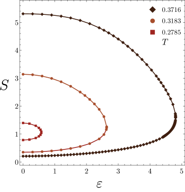
Figure 20: Entropy vs the boundary rotation parameter, when the metric is adjusted so that there is no ergoregion on the boundary. We observe two branches of black hole solutions which join up at some maximum value of $\varepsilon$.

The instabilities that we observe in the rotationally polarised AdS₄ system are primarily due to the induced ergoregion. It is interesting to ask, whether we still see instabilities if we isolate the boundary interaction term in the metric, in such a way that it does not cause the ergoregion to form. We consider the adjustment to the line elements (5) and (7a), such that $g_{tt}$ is always negative near the boundary, by choosing the reference metric in (4) to have $Q_{1}(x,y)=1+\varepsilon^{2}x^{2}(1-x^{2})^{2}(2-x^{2})y^{2}$. In this case, at any given fixed temperature $T>T^{\mathrm{Schw}}_{\min}=\sqrt{3}/(2\pi)$, we also find a maximum rotation amplitude past which we do not find stationary black hole solutions (see right panel of Fig. 20). As the system heats up, this value of $\varepsilon$ appears to increase without a bound. We also find a soliton solution, which appears to exist for any value of the rotation amplitude. We have been able to reach $\varepsilon=32$, and believe that the solution exists for any value of $\varepsilon$.

9 Conclusions and Outlook

We have used the gauge/gravity duality to study the behaviour of a strongly coupled field theory on a fixed rotating spacetime. Since our bulk field theory depends only on the metric, it lies in the universal sector of AdS/CFT. In particular, it can be embedded into a full top-down model for AdS/CFT, such as ABJM Aharony:2008ug . We restricted attention to boundary spacetimes taking the following form

$$\mathrm{d}s^{2}_{\partial}=-\mathrm{d}t^{2}+\mathrm{d}\theta^{2}+\sin^{2}\theta(\mathrm{d}\phi+\varepsilon\,\cos\theta\,\mathrm{d}t)^{2}\,,$$

and studied the behaviour of several one point functions, such as the expectation value of the stress energy tensor, for several values of $\varepsilon$. We have considered both the vacuum state and the thermal state for each value of $\varepsilon$. The holographic dual of the latter contains a black hole solution in the interior of the bulk spacetime, setting the temperature of the field theory Witten:1998qj .

We have seen that both the thermal and the vacuum states are non-unique; for a fixed angular boundary profile and fixed energy, more than one solution exists in the bulk. For boundary profiles containing ergoregions, we have observed a rather interesting behaviour. Specifically, singular black hole solutions exist, extending from the bulk all the way to the boundary, whenever the boundary profile has an evanescent ergosurface, i.e. when $\partial/\partial t$ becomes null along the equator at the boundary, but is everywhere else timelike. Furthermore, we have given ample numerical evidence that above a certain value of ${\varepsilon=\varepsilon_{c}\simeq 2.565}$, no axially symmetric stationary bulk solution exists. This value happens to always be larger than the critical value needed to generate hair. Finally, we provided a first principle derivation of the superradiant bound, i.e. we determined the minimum value of $\varepsilon$ that makes our system develop hair, purely from CFT data.

The most interesting question raised by our work does not yet have a definite answer. Namely, what happens if we start in the vacuum of the theory, i.e. pure global AdS₄, and promote $\varepsilon$ to be a function of time. In the most interesting scenario, we would increase $\varepsilon$ to a value above $\varepsilon_{c}$ and monitor the bulk dynamical evolution. We have provided numerical evidence that there are no axially symmetric and stationary solutions above this critical value. We have further seen that both the solitonic and the black hole phases can develop hair for $\varepsilon>2$. There are a number of possibilities for the nonlinear evolution of our system:

1. The superradiant instability quickly controls the dynamics, and the subsequent evolution proceeds just as described in Dias:2011at ; Dias:2015rxy ; Niehoff:2015oga .

2. A bulk horizon forms, becomes hot and expands all the way to the boundary, reaching the boundary in a finite amount of time. This is reminiscent of what was observed in Bosch:2017ccw ; Buchel:2017map .

3. A bulk horizon forms, the curvature grows large in the bulk as a power law in time, until the superradiant instability kicks in and controls the dynamics. This scenario is very similar to the one presented in Crisford:2017zpi ; 2017arXiv170907880C .

4. No horizon forms, and the curvature grows large in the bulk as a power law in time, until the superradiant instability kicks in and controls the dynamics. This scenario is again very similar to the one presented in Crisford:2017zpi ; 2017arXiv170907880C .

We do not know which one of these possibilities is most likely, but were possibility 2 to be the correct one, we would suspect that for our class of boundary metrics no positivity of energy theorem could be proven.

There are several extensions of our work that deserve attention. First, it would be interesting to consider a generalisation of this work to the Poincaré patch of AdS₄. Work in this direction will be presented elsewhere. Second, it would be interesting to understand whether the behaviour we observe depends on the rotation profile we choose. We think that most of what we reported should not be dependent on the choice of the boundary profile. For instance, we certainly believe that no solution should exist for arbitrarily large amplitudes of the boundary profile, so long as $\partial_{t}$ becomes spacelike.

Appendix A Numerical validity

We verified that our solutions satisfy $\xi^{\mu}=0$ to sufficient precision. In order to compute the stress energy tensor, adequate precision is required as we need to obtain third derivatives about the conformal boundary. We found that double precision was adequate thus significantly speeding up our computation. Nevertheless, we checked that the results converge as expected when the precision is increased.

We monitor convergence of our numerical method by computing the infinity norm of the DeTurck vector $\mathinner{\!\left\lVert\xi\right\rVert}_{\infty}$, as well as relative errors of physical quantities of interest defined by $\Delta_{N}G=\left|1-G_{N+1}/G_{N}\right|$, where $G_{N}$ denotes the quantity computed with $N$ grid points on each integration domain. This provides a good check of the numerics, as well as a measure of the error. We present convergence results for free energy in Fig. 21 which, in this work, is the physical quantity which exhibits the largest error. As $\varepsilon$ increases, the grid size has to be increased accordingly to maintain satisfactory error and typically a $60\times 60$ to $100\times 100$ grid was used. For the dominant soliton branch, $\mathinner{\!\left\lVert\xi\right\rVert}^{2}_{\infty}$ is never above $10^{-10}$ and errors in quantities never above $0.01\%$. For the large branch, $\mathinner{\!\left\lVert\xi\right\rVert}^{2}_{\infty}<10^{-7}$, and the errors are below $1\%$. For the large black holes, we keep $\mathinner{\!\left\lVert\xi\right\rVert}^{2}_{\infty}<10^{-9}$ and $\Delta_{N}G<0.01\%$, and for the small branch, $10^{-7}$ and $1\%$ respectively. Generally, we found that errors increase with both increasing and decreasing the temperature.

For analytic functions, we expect the pseudospectral methods to offer exponential convergence with an increasing grid size. However, we cannot attain these rates of convergence if the error drops below the machine precision. The error settles to an exponential decay until it starts to pivot around the machine error, and this interval is shown in Fig. 21. In order to improve convergence it is then necessary to increase numerical precision.

Figure 21: Top left: Log–linear plot of the DeTurck norm squared for the dominating soliton branch, at $\varepsilon=2.5$. Straight line indicates exponential convergence. Top right: Log–linear plot of the relative error in the free energy $G$ vs the grid size $n$, for the same data set as top left. Bottom left: Log–linear plot of the DeTurck norm squared vs grid size for a large black hole with $T=1/\pi$ and $\varepsilon=1.9875$. Bottom right: Log–linear plot of $\Delta_{N}G$ against $n$, for a cold ($T=0.2506$), small black hole, upper small branch ($\varepsilon=2.5$).

Appendix B Additional figures

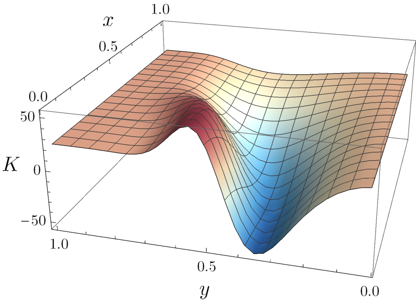
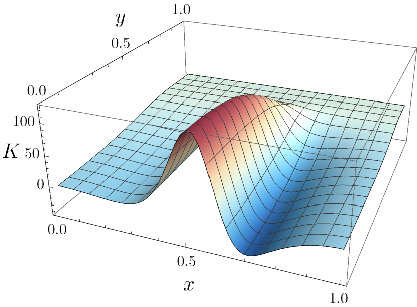
Figure 22: Left: Kretschmann scalar $K$ for the dominant soliton branch, $\varepsilon=2.564$. Right: $K$ for a large black hole with $\varepsilon=1.9$.

In Fig. 22, we present the Kretschmann scalar $K$ for a fixed value of the boundary parameter $\varepsilon\simeq\varepsilon_{c}$, where $\varepsilon_{c}$ is the maximal value up to which stationary solutions exist. The evolution of $K$ with the boundary deformation is non-trivial. In the left panel, we plot $K$ for the small soliton branch. For $\varepsilon<1.9$, the scalar has a positive minima at $y=0$, and for $\varepsilon>1.9$, it starts to display interesting features: the scalar is maximal at the equator $x=0$, displaying two large extrema close to each other, the magnitude of which are growing rapidly with the increase of the boundary rotation amplitude. At the boundary ${y=1}$, it reduces to the value of $K_{AdS}=24$, as expected for the asymptotically AdS₄ spacetimes. We also observe a local slowly increasing maxima at $y=0$, when $\varepsilon$ is large. The large, unstable, soliton branch shows a similar behavior, with magnitudes of the both extrema growing further and the distance between them decreasing, and the extrema are slowly moving towards the origin, as $\varepsilon\rightarrow 2$. There are also now two minima on each side of the maximum.

In the right panel we present the curvature scalar for the large black hole with $\varepsilon=1.9$ and $T=1/\pi$. It is maximal on the black hole horizon $y=1$, and is peaking at $\theta\rightarrow\pi/4$ as $\varepsilon\rightarrow 2$. On either side of the maximum there are two minima one of which is global. As we approach the critical amplitude, the peak, and the minima, become narrower. For $\varepsilon$ sufficiently large, the $K$ is small and positive on the poles and the equator.

Appendix C Perturbative expansion

In this section we present the perturbative expansion of the solitonic solution to order $\varepsilon^{2}$, where $\varepsilon$ is the boundary rotation parameter defined in section 2. The following procedure can be easily generalized to yield higher orders of the expansion, however the solutions become increasingly complicated. We will work in null quasi-spherical gauge Bartnik:1996js in which the solution reads

$$\begin{split}\mathrm{d}s^{2}=-\left(1+\frac{r^{2}}{L^{2}}\right)Q_{1}(r,\theta)\,\mathrm{d}t^{2}&+\left(1+\frac{r^{2}}{L^{2}}\right)^{-1}Q_{2}(r,\theta)\,\mathrm{d}r^{2}\\ &+r^{2}Q_{3}(r,\theta)\left[\mathrm{d}\theta^{2}+\sin{\theta}^{2}\left(\mathrm{d}\phi+\Omega(r,\theta)\,\mathrm{d}t\right)^{2}\right]\end{split}$$ (43)

where $\{\theta,\phi\}$ are the standard polar coordinates of unit two-sphere, and $L$ is the AdS₄ length. The gauge requires that the functions $Q_{i}$ ($i=1,2,3$) and $\Omega$ depend only on $r$ and $\theta$, and we will also use the fact that if $Q_{i}=Q_{i}(r)$ (and $\Omega=0$), we can additionally fix $Q_{3}=1$. As the induced stress-energy tensor is of order $\varepsilon^{2}$ in the angular velocity, consider an expansion in $\varepsilon$ given by

$$Q_{i}(r,\theta)=\sum_{i=0}^{+\infty}\varepsilon^{2i}q_{i}^{(2i)}(r,\theta),\qquad\qquad\Omega(r,\theta)=\sum_{i=0}^{+\infty}\varepsilon^{2i+1}\Omega^{(2i+1)}(r,\theta)$$ (44)

where we are expanding around a pure AdS₄ background given by $q_{i}^{(0)}=1$. At linear order we obtain a second order partial differential equation for $\Omega^{(1)}$ which can be solved using separation of variables subject to regularity at the origin. The solution is given by

$$\Omega^{(1)}(r,\theta)=\frac{2}{3\sqrt{\pi}}\sum_{l=0}^{+\infty}c^{(1)}_{l}\frac{\Gamma\left(\frac{l+3}{2}\right)\Gamma\left(\frac{l+5}{2}\right)}{\Gamma\left(l+\frac{5}{2}\right)}\,P_{l+1}^{\prime}(\cos{\theta})\left(\frac{r}{L}\right)^{l}\!_{2}F_{1}\left(\frac{l}{2},\frac{l+3}{2};l+\frac{5}{2};-\frac{r^{2}}{L^{2}}\right),$$ (45)

where $l$ is the harmonic number, $c^{(1)}_{l}$ are real numbers depending on the boundary profile, $P_{l}$ is Legendre polynomial of degree $l$ and $\!\,{}_{2}F_{1}$ is ordinary hypergeometric function. At the boundary the perturbation reduces to

$$\lim_{r\rightarrow+\infty}\Omega^{(1)}(r,\theta)=\sum_{l=0}^{+\infty}c^{(1)}_{l}P_{l+1}^{\prime}(\cos{\theta}),$$ (46)

and at first order the first harmonic $l=1$ gives us the dipolar boundary rotation profile ${\Omega(r,\theta)=\varepsilon\cos{\theta}}$. The final expression is

$$\Omega^{(1)}(r,\theta)=\frac{2L^{4}}{\pi r^{4}}\cos{\theta}\left[\frac{r}{L}\left(\frac{r^{2}}{L^{2}}+3\right)+\left(\frac{r^{2}}{L^{2}}-3\right)\left(\frac{r^{2}}{L^{2}}+1\right)\arctan\left(\frac{r}{L}\right)\right].$$ (47)

The first order angular velocity perturbation effectively sources the stress energy tensor at $\varepsilon^{2}$. We decompose the second order perturbations as Kodama:2003jz

$$q_{i}^{(2)}(r,\theta)=\gamma_{i}(r)+\alpha_{i}(r)P_{2}(\cos{\theta})+\beta_{i}(r)P_{4}(\cos{\theta}),$$ (48)

where the remaining gauge freedom is used to set $\gamma_{3}(r)=0$. We solve the equations requiring that the functions are regular at the origin $r=0$ and, that up to a diffeomorphism, they asymptotically satisfy AdS₄ boundary conditions. Below we provide the full perturbative functions:

$$\begin{split}&\gamma_{1}(r)=\frac{2L^{2}}{15\pi^{2}r^{6}(L^{2}+r^{2})}\left.\bigg{(}24L^{6}r^{2}+20L^{4}r^{4}-9(\pi^{2}-4)L^{2}r^{6}-8\left(6L^{7}r+7L^{5}r^{3}-6L^{3}r^{5}\right.\right.\\ &\quad\bigg{.}\left.-9Lr^{7}\right)\arctan\left(\frac{r}{L}\right)+4\left(6L^{8}+9L^{6}r^{2}+L^{4}r^{4}+7L^{2}r^{6}+9r^{8}\right)\arctan\left(\frac{r}{L}\right)^{2}-9\pi^{2}r^{8}\bigg{)},\\ &\gamma_{2}(r)=-\frac{8L^{4}}{15\pi^{2}r^{6}(L^{2}+r^{2})}\left((3L^{2}-r^{2})(L^{2}+r^{2})\arctan\left(\frac{r}{L}\right)-Lr(3L^{2}+r^{2})\right)\end{split}$$

$$\begin{split}&\hskip 230.00035pt\times\bigg{(}(3L^{2}+r^{2})\arctan\left(\frac{r}{L}\right)-3Lr\bigg{)},\\ &\alpha_{1}(r)=\frac{L^{2}}{84\pi^{2}r^{6}(L^{2}+r^{2})}\left.\bigg{(}96L^{6}r^{2}+L^{4}(-752+63\pi^{2})r^{4}+7L^{2}(-16+15\pi^{2})r^{6}\right.\\ &\qquad+\arctan\left(\frac{r}{L}\right)\left(-192L^{7}r+7L^{5}(176-9\pi^{2})r^{3}+2L^{3}(368-63\pi^{2})r^{5}+L(80-63\pi^{2})r^{7}\right.\\ &\hskip 120.00018pt\Bigg{.}\bigg{.}+32(L^{2}+r^{2})\left(3L^{6}-18L^{4}r^{2}+L^{2}r^{4}+6r^{6}\right)\arctan\left(\frac{r}{L}\right)\bigg{)}\Bigg{)},\\ &\alpha_{2}(r)=\frac{L^{3}}{84\pi^{2}r^{6}(L^{2}+r^{2})}\left(3936L^{5}r^{2}+(4208-63\pi^{2})L^{3}r^{4}+\arctan\left(\frac{r}{L}\right)\left(-7872L^{6}r+\right.\right.\\ &\qquad\left.(63\pi^{2}-10832)L^{4}r^{3}+2(63\pi^{2}-944)L^{2}r^{5}+32L(L^{2}+r^{2})\left(123L^{4}+84L^{2}r^{2}-23r^{4}\right)\right.\\ &\hskip 140.00021pt\Bigg{.}\bigg{.}\times\arctan\left(\frac{r}{L}\right)+(304+63\pi^{2})r^{7}\bigg{)}+(304-105\pi^{2})Lr^{6}\Bigg{)},\\ &\alpha_{3}(r)=\frac{L^{2}}{84\pi^{2}r^{6}}\left(-384L^{4}r^{2}-7(64+9\pi^{2})L^{2}r^{4}+\arctan\left(\frac{r}{L}\right)\left(768L^{5}r+(1360+63\pi^{2})\right.\right.\\ &\times L^{3}r^{3}-48\left(8L^{6}+19L^{4}r^{2}-10L^{2}r^{4}+3r^{6}\right)\arctan\left(\frac{r}{L}\right)-(592+63\pi^{2})Lr^{5}\bigg{)}+84\pi^{2}r^{6}\Bigg{)},\\ &\beta_{1}(r)=\frac{L^{2}}{1680\pi^{2}r^{6}(L^{2}+r^{2})}\left.\Bigg{(}3(5408+735\pi^{2})L^{6}r^{2}+38(608+105\pi^{2})L^{4}r^{4}\right.\\ &\qquad\quad+21(224+81\pi^{2})L^{2}r^{6}+\arctan\left(\frac{r}{L}\right)\left(3(1504-735\pi^{2})L^{7}r+63(352-75\pi^{2})L^{5}r^{3}\right.\\ &\qquad\left.+3(7712-945\pi^{2})L^{3}r^{5}-256(L^{2}+r^{2})\left(81L^{6}+144L^{4}r^{2}+48L^{2}r^{4}+r^{6}\right)\arctan\left(\frac{r}{L}\right)\right.\\ &\hskip 285.00043pt\Bigg{.}+(4448-315\pi^{2})Lr^{7}\Bigg{)},\\ &\beta_{2}(r)=\frac{L^{3}}{1680\pi^{2}r^{6}(L^{2}+r^{2})}\Bigg{(}-3(32+735\pi^{2})L^{5}r^{2}-2(3104+1995\pi^{2})L^{3}r^{4}\Bigg{.}\\ &\hskip 115.00017pt+\arctan\left(\frac{r}{L}\right)\bigg{(}3(735\pi^{2}-12256)L^{6}r+15(315\pi^{2}-4448)L^{4}r^{3}\\ &\hskip 90.00014pt\left.+(2835\pi^{2}-35936)L^{2}r^{5}+256L(L^{2}+r^{2})\left(144L^{4}+189L^{2}r^{2}+61r^{4}\right)\right.\\ &\hskip 127.00015pt\Bigg{.}\bigg{.}\times\arctan\left(\frac{r}{L}\right)+5(63\pi^{2}-992)r^{7}\bigg{)}-(4960+1701\pi^{2})Lr^{6}\Bigg{)},\\ &\beta_{3}(r)=\frac{L^{2}}{1680\pi^{2}r^{6}}\left(-3L^{4}(7072+735\pi^{2})r^{2}+7L^{2}(544-45\pi^{2})r^{4}+224\pi^{2}r^{6}\right.\\ &\qquad\quad+\arctan\left(\frac{r}{L}\right)\left(9L^{5}(608+245\pi^{2})r+2L^{3}(-5536+525\pi^{2})r^{3}+L(2656-315\pi^{2})r^{5}\right.\\ &\hskip 130.0002pt\Bigg{.}\bigg{.}+128\left(123L^{6}+153L^{4}r^{2}-19L^{2}r^{4}-9r^{6}\right)\arctan\left(\frac{r}{L}\right)\bigg{)}\Bigg{)}.\end{split}$$ (49)

Using this second order expansion we compute thermodynamic quantities, and test the first law (see subsec. 4.4). We also find equilibrium conditions for spinning test particles on the rotation axis $\theta=0$. For the metric (43), the spin to mass ratio (see sec. 7) is given by

$$\frac{S}{M}=\frac{\pi r^{6}}{16\varepsilon L^{2}\sqrt{r^{2}+1}\left[\left(3L^{2}+r^{2}\right)\tan^{-1}\left(r/L\right)-3Lr\right]}+\mathcal{O}(\varepsilon),$$ (50)

and vanishes when $r\rightarrow 0$. The comparison with the full non-linear numerical results are presented in Fig. 18.

References

- (1) S. W. Hawking, Black hole explosions, Nature 248 (1974) 30–31.
- (2) J. M. Maldacena, The Large N limit of superconformal field theories and supergravity, Int.J.Theor.Phys. 38 (1999) 1113–1133, [hep-th/9711200].
- (3) S. S. Gubser, I. R. Klebanov, and A. M. Polyakov, Gauge theory correlators from noncritical string theory, Phys. Lett. B428 (1998) 105–114, [hep-th/9802109].
- (4) E. Witten, Anti-de Sitter space and holography, Adv. Theor. Math. Phys. 2 (1998) 253–291, [hep-th/9802150].
- (5) O. Aharony, S. S. Gubser, J. M. Maldacena, H. Ooguri, and Y. Oz, Large N field theories, string theory and gravity, Phys. Rept. 323 (2000) 183–386, [hep-th/9905111].
- (6) Y. B. Zeldovich, Generation of Waves by a Rotating Body, JETP Lett. 14 (1971) 180.
- (7) Y. B. Zeldovich, Amplification of cylindrical electromagnetic waves reflected from a rotating body, Sov. Phys. JETP 35 (1972) 1085.
- (8) W. H. Press and S. A. Teukolsky, Floating Orbits, Superradiant Scattering and the Black-hole Bomb, Nature 238 (1972) 211–212.
- (9) A. A. Starobinsky and S. M. Churilov, Amplification of waves during reflection from a rotating black hole, Sov. Phys. JETP 37 (1973) 28.
- (10) A. A. Starobinsky and S. M. Churilov, Amplification of electromagnetic and gravitational waves scattered by a rotating black hole, Sov. Phys. JETP 38 (1973) 1.
- (11) S. L. Detweiler and J. R. Ipser, Stability of scalar perturbations of a Kerr-metric black hole, Astrophys. J. 185 (1973) 675–683.
- (12) T. J. M. Zouros and D. M. Eardley, Instabilities of Massive Scalar Perturbations of a Rotating Black Hole, Annals Phys. 118 (1979) 139–155.
- (13) S. L. Detweiler, Klein-Gordon Equation and Rotating Black Holes, Phys. Rev. D22 (1980) 2323–2326.
- (14) H. K. Kunduri, J. Lucietti, and H. S. Reall, Gravitational perturbations of higher dimensional rotating black holes: Tensor perturbations, Phys. Rev. D74 (2006) 084021, [hep-th/0606076].
- (15) Ó. J. C. Dias, G. T. Horowitz, and J. E. Santos, Black holes with only one Killing field, JHEP 07 (2011) 115, [arXiv:1105.4167].
- (16) Ó. J. C. Dias and J. E. Santos, Boundary Conditions for Kerr-AdS Perturbations, JHEP 10 (2013) 156, [arXiv:1302.1580].
- (17) V. Cardoso, Ó. J. C. Dias, G. S. Hartnett, L. Lehner, and J. E. Santos, Holographic thermalization, quasinormal modes and superradiance in Kerr-AdS, JHEP 04 (2014) 183, [arXiv:1312.5323].
- (18) C. A. R. Herdeiro and E. Radu, Kerr black holes with scalar hair, Phys. Rev. Lett. 112 (2014) 221101, [arXiv:1403.2757].
- (19) Ó. J. C. Dias, J. E. Santos, and B. Way, Black holes with a single Killing vector field: black resonators, JHEP 12 (2015) 171, [arXiv:1505.04793].
- (20) B. E. Niehoff, J. E. Santos, and B. Way, Towards a violation of cosmic censorship, Class. Quant. Grav. 33 (2016), no. 18 185012, [arXiv:1510.00709].
- (21) S. W. Hawking and D. N. Page, Thermodynamics of Black Holes in anti-De Sitter Space, Commun. Math. Phys. 87 (1983) 577.
- (22) O. Aharony, O. Bergman, D. L. Jafferis, and J. Maldacena, N=6 superconformal Chern-Simons-matter theories, M2-branes and their gravity duals, JHEP 10 (2008) 091, [arXiv:0806.1218].
- (23) L. Lehner and F. Pretorius, Black Strings, Low Viscosity Fluids, and Violation of Cosmic Censorship, Phys. Rev. Lett. 105 (2010) 101102, [arXiv:1006.5960].
- (24) P. Figueras, M. Kunesch, and S. Tunyasuvunakool, End Point of Black Ring Instabilities and the Weak Cosmic Censorship Conjecture, Phys. Rev. Lett. 116 (2016), no. 7 071102, [arXiv:1512.04532].
- (25) P. Figueras, M. Kunesch, L. Lehner, and S. Tunyasuvunakool, End Point of the Ultraspinning Instability and Violation of Cosmic Censorship, Phys. Rev. Lett. 118 (2017), no. 15 151103, [arXiv:1702.01755].
- (26) J. W. York, Jr., Role of conformal three geometry in the dynamics of gravitation, Phys. Rev. Lett. 28 (1972) 1082–1085.
- (27) G. W. Gibbons and S. W. Hawking, Action Integrals and Partition Functions in Quantum Gravity, Phys. Rev. D15 (1977) 2752–2756.
- (28) S. R. Green, S. Hollands, A. Ishibashi, and R. M. Wald, Superradiant instabilities of asymptotically anti-de Sitter black holes, Class. Quant. Grav. 33 (2016), no. 12 125022, [arXiv:1512.02644].
- (29) M. Headrick, S. Kitchen, and T. Wiseman, A New approach to static numerical relativity, and its application to Kaluza-Klein black holes, Class.Quant.Grav. 27 (2010) 035002, [arXiv:0905.1822].
- (30) T. Wiseman, Numerical construction of static and stationary black holes, in Black Holes in Higher Dimensions, ch. 10, pp. 233–279. Cambridge University Press, 2012.
- (31) Ó. J. C. Dias, J. E. Santos, and B. Way, Numerical methods for finding stationary gravitational solutions, Classical and Quantum Gravity 33 (July, 2016) 133001, [arXiv:1510.02804].
- (32) P. Figueras and T. Wiseman, On the existence of stationary Ricci solitons, Class. Quant. Grav. 34 (2017), no. 14 145007, [arXiv:1610.06178].
- (33) J. Markevičiūtė, and J. E. Santos, Hairy black holes in AdS, JHEP 06 (2016) 096, [arXiv:1602.03893].
- (34) G. W. Gibbons, C. A. R. Herdeiro, and C. Rebelo, Global embedding of the Kerr black hole event horizon into hyperbolic 3-space, Phys. Rev. D80 (2009) 044014, [arXiv:0906.2768].
- (35) J. D. Brown and J. W. York, Jr., Quasilocal energy and conserved charges derived from the gravitational action, Phys. Rev. D47 (1993) 1407–1419, [gr-qc/9209012].
- (36) M. Henningson and K. Skenderis, The Holographic Weyl anomaly, JHEP 07 (1998) 023, [hep-th/9806087].
- (37) V. Balasubramanian and P. Kraus, A Stress tensor for Anti-de Sitter gravity, Commun. Math. Phys. 208 (1999) 413–428, [hep-th/9902121].
- (38) S. de Haro, S. N. Solodukhin, and K. Skenderis, Holographic reconstruction of space-time and renormalization in the AdS / CFT correspondence, Commun. Math. Phys. 217 (2001) 595–622, [hep-th/0002230].
- (39) V. Iyer and R. M. Wald, Some properties of Noether charge and a proposal for dynamical black hole entropy, Phys. Rev. D50 (1994) 846–864, [gr-qc/9403028].
- (40) I. Papadimitriou and K. Skenderis, Thermodynamics of asymptotically locally AdS spacetimes, JHEP 08 (2005) 004, [hep-th/0505190].
- (41) G. Compere, Note on the First Law with p-form potentials, Phys. Rev. D75 (2007) 124020, [hep-th/0703004].
- (42) A. Chamblin, R. Emparan, C. V. Johnson, and R. C. Myers, Charged AdS black holes and catastrophic holography, Phys. Rev. D60 (1999) 064018, [hep-th/9902170].
- (43) A. Chamblin, R. Emparan, C. V. Johnson, and R. C. Myers, Holography, thermodynamics and fluctuations of charged AdS black holes, Phys. Rev. D60 (1999) 104026, [hep-th/9904197].
- (44) G. T. Horowitz and V. E. Hubeny, Quasinormal modes of AdS black holes and the approach to thermal equilibrium, Phys. Rev. D62 (2000) 024027, [hep-th/9909056].
- (45) A. Donos and J. P. Gauntlett, Holographic Q-lattices, JHEP 04 (2014) 040, [arXiv:1311.3292].
- (46) M. S. Costa, L. Greenspan, M. Oliveira, J. Penedones, and J. E. Santos, Polarised Black Holes in AdS, Class. Quant. Grav. 33 (2016), no. 11 115011, [arXiv:1511.08505].
- (47) R. Wald, Gravitational spin interaction, Phys. Rev. D 6 (Jul, 1972) 406–413.
- (48) J. Natario, Quasi-Maxwell interpretation of the spin-curvature coupling, Gen. Rel. Grav. 39 (2007) 1477–1487, [gr-qc/0701067].
- (49) L. F. O. Costa, J. Natário, and M. Zilhão, Spacetime dynamics of spinning particles: Exact electromagnetic analogies, Phys. Rev. D 93 (May, 2016) 104006.
- (50) M. Mathisson, Republication of: New mechanics of material systems, General Relativity and Gravitation 42 (2010), no. 4 1011–1048.
- (51) A. Papapetrou, Spinning test-particles in general relativity., Proceedings of the Royal Society of London A: Mathematical, Physical and Engineering Sciences 209 (1951), no. 1097 248–258.
- (52) F. A. E. Pirani, On the Physical significance of the Riemann tensor, Acta Phys. Polon. 15 (1956) 389–405. [Gen. Rel. Grav.41,1215(2009)].
- (53) W. Tulczyjew, Motion of multipole particles in general relativity theory, Acta Phys. Pol. 18 (1959) 393.
- (54) A. H. Taub, Motion of test bodies in general relativity, Journal of Mathematical Physics 5 (1964), no. 1 112–119, [http://dx.doi.org/10.1063/1.1704055].
- (55) W. G. Dixon, A covariant multipole formalism for extended test bodies in general relativity, Il Nuovo Cimento (1955-1965) 34 (1964), no. 2 317–339.
- (56) W. G. Dixon, Dynamics of extended bodies in general relativity, Proceedings of the Royal Society of London A: Mathematical, Physical and Engineering Sciences 314 (1970), no. 1519 499–527.
- (57) O. Semerák, Spinning test particles in a Kerr field - I, MNRAS 308 (Sept., 1999) 863–875.
- (58) C. M ller, On the definition of the centre of gravity of an arbitrary closed system in the theory of relativity, Commun. Dublin Inst. Adv. Stud. 5 (1949), no. 42.
- (59) B. Carter, Hamilton-jacobi and schr dinger separable solutions of einstein’s equations, Comm. Math. Phys. 10 (1968), no. 4 280–310.
- (60) M. S. Costa, L. Greenspan, J. Penedones, and J. E. Santos, Polarised black holes in ABJM, Journal of High Energy Physics 6 (June, 2017) 24, [arXiv:1702.04353].
- (61) M. S. Costa, L. Greenspan, M. Oliveira, J. Penedones, and J. E. Santos, Polarised black holes in AdS, Classical and Quantum Gravity 33 (June, 2016) 115011, [arXiv:1511.08505].
- (62) P. Bosch, A. Buchel, and L. Lehner, Unstable horizons and singularity development in holography, JHEP 07 (2017) 135, [arXiv:1704.05454].
- (63) A. Buchel, Singularity development and supersymmetry in holography, JHEP 08 (2017) 134, [arXiv:1705.08560].
- (64) T. Crisford and J. E. Santos, Violating the Weak Cosmic Censorship Conjecture in Four-Dimensional Anti-de Sitter Space, Phys. Rev. Lett. 118 (2017), no. 18 181101, [arXiv:1702.05490].
- (65) T. Crisford, G. T. Horowitz, and J. E. Santos, Testing the Weak Gravity - Cosmic Censorship Connection, ArXiv e-prints (Sept., 2017) [arXiv:1709.07880].
- (66) R. Bartnik, Einstein equations in the null quasispherical gauge, Class. Quant. Grav. 14 (1997) 2185–2194, [gr-qc/9611045].
- (67) H. Kodama and A. Ishibashi, A Master equation for gravitational perturbations of maximally symmetric black holes in higher dimensions, Prog. Theor. Phys. 110 (2003) 701–722, [hep-th/0305147].