CERN-TH-2018-093

Probing large-scale magnetism

with the Cosmic Microwave Background

Massimo Giovannini

Department of Physics, Theory Division, CERN, 1211 Geneva 23, Switzerland
INFN, Section of Milan-Bicocca, 20126 Milan, Italy

Abstract

Prior to photon decoupling magnetic random fields of comoving intensity in the nano-Gauss range distort the temperature and the polarization anisotropies of the microwave background, potentially induce a peculiar $B$-mode power spectrum and may even generate a frequency-dependent circularly polarized $V$-mode. We critically analyze the theoretical foundations and the recent achievements of an interesting trialogue involving plasma physics, general relativity and astrophysics.

1 A magnetized Universe

1.1 History, orders of magnitude and units

At the dawn of the seventeenth century William Gilbert published a celebrated treatise entitled De Magnete, Magneticisque Corporibus, et de Magno Magnete Tellure [1] where the quest for a coherent presentation of electric and magnetic phenomena anticipated the spirit, if not the letter, of the Maxwellian unification. In his systematic effort, Gilbert even conjectured that large-scale magnets (like the earth itself) could share the same physical properties of magnetic phenomena over much shorter distance-scales: a similar kind of extrapolation is at the heart of modern astrophysical applications from planetary sciences to black-holes. More than two hundred years later Michael Faraday introduced the expression magnetic field, a wording coined by Faraday himself while summarizing an amazing series of observations in his Experimental Researches in Electricity [2]. Since then, the synergic evolution of physics, astronomy and astrophysics has been guided in many cases by the study of magnetic fields over different length-scales so that today nearly all astrophysical objects, from planets to clusters of galaxies, appear to be magnetized, at least to a certain degree. Through the years the quantity and quality of the answerable questions became larger and now we are allowed to ask sensible questions on the origin of large-scale magnetism with the hope of receiving reasonably definite answers. The present discussion, with its own limitations, aims at summarizing in a theoretical perspective the various interesting attempts involving the interplay between large-scale magnetism and the physics of the microwave background.

Physical system	Magnetic field intensity	Typical scale of variation
earth	${\mathcal{O}}(1)$ G	${\mathcal{O}}(10^{4}\,\mathrm{km})$
Jupiter	${\mathcal{O}}(10)$ G	${\mathcal{O}}(10^{5}\mathrm{km})$
LHC dipoles	${\mathcal{O}}(10^{5})$ G	${\mathcal{O}}(15\,\mathrm{m})$
neutron stars	${\mathcal{O}}(10^{13})$ G	${\mathcal{O}}(10\,\mathrm{km})$
spiral galaxies	${\mathcal{O}}(10^{-6})$ G	${\mathcal{O}}(30\,\mathrm{kpc})$
regular (Abell) clusters	${\mathcal{O}}(10^{-7})$ G	$<{\mathcal{O}}(\mathrm{Mpc})$

Table 1: The magnetic field intensities of different physical systems are compared in terms of their associated scales of variation.

The magnetic fields of physical systems characterized by very different scales of variation are compared in Tab. 1. The scale of variation roughly measures the distance over which there is an appreciable correlation between the values of the field at two spatially separated points. The dipoles of the Large Hadron Collider (LHC) are of the order of $10^{5}$ G, that is to say almost a million times larger that the earth’s magnetic field which is roughly $0.3$ G. From Tab. 1 we also see that the geomagnetic field (as well as the magnetic fields of other planets of the solar system) is a million times more intense than the magnetic fields of the galaxies and of the intergalactic medium. One of the largest magnetic field intensities we can plausibly imagine in the framework of quantum electrodynamics comes from the Schwinger threshold for the production of electron-positron pairs demanding, at least, a field $m_{e}^{2}/e$ (where $m_{e}$ is the electron mass and $e$ the corresponding charge). The Schwinger limit implies an intensity of the order of $10^{13}$ G that is comparable, according to Tab. 1 with the magnetic fields possibly present at the surface of a neutron star. The rationale for the huge magnetic fields of neutron stars may be what we call compressional amplification: since at high conductivity the magnetic flux is frozen into the plasma element, as the gravitational collapse takes place the magnetic field increases. We shall preferentially measure magnetic fields in Gauss within the natural system of units (i.e. $\hbar=c=k_{B}=1$, where $k_{B}$ is the Boltzmann constant). In these units the Bohr magneton equals $5.788\times 10^{-11}{\rm MeV}/{\rm Tesla}$ and the relation between Tesla, Gauss and GeV is given by the following equations

$$1\,{\rm Tesla}=10^{4}\,{\rm Gauss},\qquad 1\,\mathrm{Gauss}=6.9241\times 10^{-20}\,\mathrm{GeV}^{2}.$$ (1.1)

W shall often employ the well known metric prefixes to indicate the multiples (or the fractions) of a given unit; so for instance, $\mu\mathrm{G}=10^{-6}\,\mathrm{G}$, $\mathrm{nG}=10^{-9}\mathrm{G}$ and so on. When needed the typical length-scales will be often expressed in parsec and their multiples: recall, in this respect, that $1\,\mathrm{kpc}=3.085\times 10^{21}\mathrm{cm}$. The present value of the Hubble radius is $H_{0}^{-1}=4282.7\,(h_{0}/0.7)\,\mathrm{Mpc}$. Magnetic fields whose correlation length is larger than the astronomical unit ( $1\,{\rm AU}=1.49\times 10^{13}{\rm cm}$) will be referred to as large-scale magnetic fields. While this choice is largely conventional, magnetic fields with approximate correlation scale comparable with the earth-sun distance are not observed (on the contrary, both the magnetic field of the sun and the one of the earth have a clearly distinguishable localized structure). Furthermore simple magnetohydrodynamical estimates seem to suggest that the magnetic diffusivity scale (i.e. the scale below which magnetic fields are diffused because of the finite value of the conductivity of the corresponding medium) of the order of the AU. For a definition of the magnetic diffusivity scale in weakly interacting plasmas see, for instance, section 2.1 and discussion therein.

The central theme of this paper deals with two apparently unrelated phenomena, namely the large-scale magnetism and the Cosmic Microwave Background radiation (CMB in what follows) originally discovered by Penzias and Wilson [3] and subsequently confirmed by the COBE satellite mission [4, 5, 6] which also gave the first solid evidence of the large-scale temperature anisotropies. The CMB temperature is given by [7]:

$$T_{\gamma 0}=(2.72548\pm 0.00057)\,\mathrm{K}.$$ (1.2)

The energy density of the CMB turns out to be of the same order of the energy density of the magnetic energy density stored in the galactic field. More specifically we could say

$$\rho_{\gamma 0}=\frac{\pi^{2}}{15}T_{\gamma 0}^{4}=2.001\times 10^{-51}\,\,\biggl{(}\frac{T_{\gamma 0}}{2.72548}\biggr{)}^{4}\,\,\mathrm{GeV}^{4},$$ (1.3)

$$\rho_{\mathrm{B}}=\frac{B^{2}}{8\pi}=2.002\times 10^{-51}\biggl{(}\frac{B}{3.24\mu\mathrm{G}}\biggr{)}^{2}\,\,\mathrm{GeV}^{4},$$ (1.4)

where Eq. (1.1) has been used together with the conversion between K degrees and eV. Equations (1.3) and (1.4) just account for an interesting numerical coincidence. Needless to say that the galactic magnetic field is not exactly $3.24\,\mu\mathrm{G}$: the magnetic field in the Solar neighbourhood has regular component and a random contribution so that estimates of the total magnetic field, depending on the way we count, range between $2$ and $6\mu\mathrm{G}$ [8]. It is however relevant to stress that the energy density of the CMB, the energy density of the galactic magnetic field and the energy density of the cosmic rays are all comparable within one order of magnitude. Two excellent background monographs on large-scale magnetism are listed in Refs. [9, 10].

1.2 Magnetic fields in galaxies

While it is probably true that large-scale magnetism is the birthright of radio-astronomy, the very first evidence of galactic and interstellar magnetic fields came from the isotropy of the galactic cosmic ray spectrum in the Milky Way and from the polarization of starlight. The lack of detection of appreciable anisotropies in cosmic ray spectrum led Fermi [11] to suggest the existence of a magnetic field of approximate $\mu$G strength scrambling the trajectories of the charged particles and making the spectrum fairly isotropic. Even if concrete evidences of large-scale magnetic fields in the interstellar media were still lacking, magnetic fields were known to be stable in highly conducting plasmas thanks to the seminal contributions of Alfvén [12]. Few months after Fermi’s proposal Hiltner [15] and, independently, Hall [16] observed the polarization of starlight which was later on interpreted by Davis and Greenstein [17] as an effect of galactic magnetic field aligning the dust grains.

After more than three score years of radio-astronomical observations, spiral galaxies are known to have magnetic fields in the same range of the Milky Way (i.e. ${\mathcal{O}}(\mu\mathrm{G})$) while elliptical galaxies have similar intensities but shorter correlation scales. As already alluded to in connection with Eqs. (1.3)–(1.4), galaxies have a regular magnetic field but they also possess a random component: magnetized domains with typical correlation scales from $100$ pc to few kpc are observed in the galactic halo of the Milky Way. Two excellent background monographs on galactic magnetism can be found in Refs. [18, 19]. In the last decade or so it has been established that planets and stars are formed in an environment which is already magnetized [20, 21] so that, as lucidly argued in a comprehensive review on large-scale magnetism [22], the true question before us today does not concern the existence of these fields but rather their origin. The measurements of galactic magnetic fields in the Milky Way and in external galaxies are reviewed in various papers (see e.g. [22, 23, 24] and [25] for an introduction to the main observational techniques). It is often difficult to disentangle the large-scale (ordered) fields from other components with smaller correlations scales. In this respect newly developed spectropolarimetric techniques [26] for wide-band polarization observations might not only improve the sensitivity but also give synthesized maps of Faraday rotation measure.

It is at the moment not yet clear if the observed galactic fields are the consequence of a strong dynamo action (see e.g. [9, 10, 19]) or if their existence somehow precedes the formation of galaxies. According to some intriguing suggestions, if the magnetic fields do not flip their sign from one spiral arm to the other, then a strong dynamo action can be suspected [23] (see also [24]). In the opposite case the magnetic field of galaxies should (or could) be primordial (i.e. present already at the onset of gravitational collapse). In this perespective a further indication that would support the primordial nature of the magnetic field of galaxies would be, for instance, the evidence that not only spirals but also elliptical galaxies are magnetized with a correlation scale shorter than in the case of spirals. Since elliptical galaxies have a much less efficient rotation, it seems difficult to postulate a strong dynamo action as the common origin of the two corresponding magnetic fields.

1.3 Magnetic fields in clusters

Magnetic fields are not only associated with galaxies but also with clusters which are gravitationally bound systems of galaxies. The Milky Way is part of the local group which is our own cluster and other members of the local group (e.g. Andromeda and Magellanic clouds) have magnetic fields between few and $10$ $\mu\mathrm{G}$. While the local group contains fewer members than other rich clusters (and it is sometimes referred to as an irregular cluster), regular clusters (like the Coma cluster) are magnetized at a level of $0.5\,\mu\mathrm{G}$ for typical correlation scales between $500$ kpc and the Mpc. Magnetic fields of single clusters have been extensively analyzed but in the last decade or so remarkable analyses of multi-cluster measurements became available [27] (see also [22, 28] for review articles on these specific themes). In the past it was shown that regular clusters have cores with a detectable component of Faraday rotation measure. There is now mounting evidence that $\mu\mathrm{G}$ magnetic fields are indeed detected inside regular Abell clusters [29, 30], as originally suggested in [28].

Weakly bound systems of clusters (i.e. superclusters) have been also claimed to be magnetized at the $\mu\mathrm{G}$ level: this is the case for the local supercluster (formed by the local group and by the Virgo cluster) and for the Coma supercluster [31]. The current indications seem to be encouraging even if crucial ambiguities persist on the way the magnetic field strengths are inferred from the Faraday rotation measurements of superclusters magnetic fields. It is not excluded that the recent progress in spectropolarimetric techniques [26] could be used also in the case of superclusters. In this connection we can mention that the intergalactic magnetic field in cosmic voids can be indirectly probed through its effect on electromagnetic cascades initiated by a source of TeV gamma-rays, such as active galactic nuclei. The original idea of Plaga [32, 33] suggested the possibility of deriving lower limits on the magnetic fields in voids even if reasonable statistical analyses seem to cast doubts on the claimed lower limits [34].

The hope for the near future is connected with the possibility of a next generation radio-telescope like the Square Kilometer Array (for short SKA [35]). The unprecedented collecting area of the instrument and the frequency range (hopefully between $0.1$–$25$ GHz) will allow full sky surveys of Faraday Rotation which may be combined with the most recent advances spectro-polarimetry [26]. This instrument might not only be directly beneficial for the microwave background physics but it might also have an amazing impact in pulsar searches [36] which are essential for sound determinations of magnetic fields from Faraday rotation [22, 23, 24, 25].

To close the circle we can go back to the isotropy of the cosmic ray spectrum and remind that nearly ten years ago the Auger collaboration advertized a correlation between the arrival directions of cosmic rays with energy above $6\times 10^{19}$ eV and the positions of active galactic nuclei within 75 Mpc [37]. In the same context concurrent analyses demonstrated [38] that overdensities on windows of 5 degree radius (and for energies $10^{17.9}eV<E<10^{18.5}$ eV) were compatible with an isotropic distribution. In a nutshell the claim was that in the highest energy domain (i.e. energies larger than $60$ EeV) cosmic rays were not appreciably deflected: within a cocoon of 70 Mpc the intensity of the (uniform) component of the putative magnetic field should be smaller than ${\mathcal{O}}(\mathrm{nG})$. The evidence of this claim got worse and worse so that the recent analyses suggest [39] that no deviation from isotropy is observed on any angular scale in the energy range between $4$ and $8$ EeV. Above $8$ EeV a weak indication for a dipole moment is claimed; no other deviation from isotropy is observed for other moments. While the claimed departure from isotropy is still at the level of indication, if cosmic rays would also be roughly isotropic in the EeV range, it would be tempting to conclude for the existence of potentially large magnetic fields (in the $10$ or $100$ nG range) for typical correlation scales larger than $10$ Mpc. It is amusing to note that the speculations of a single source accounting for a nearly isotropic high-energy cosmic ray spectrum in the presence of strong magnetic fields [40] now are becoming more plausible.

1.4 Magnetic fields at the largest scales

In spite of the remarkable progresses of the last decade, as we probe larger and larger distance scales the techniques used in the case of galaxies and clusters (i.e. Faraday rotation measures or synchrotron emission) become ambiguous. Therefore if we aim at scrutinizing the magnetization of the whole Universe we need to investigate directly the microwave background and its anisotropies.

The idea of employing microwave background physics as a magnetometer has a relatively long history which should be traced back to the seminal contributions of Hoyle [41] and Zeldovich [42]. Less than ten years after the debate that confirmed the existence of a magnetic field associated with the galaxy [11, 13, 14], Hoyle speculated in favour of a cosmological origin for the galactic magnetic fields and mentioned CMB physics as a crucial test of his idea. In a contribution entirely devoted to the steady state theory [41], Hoyle discussed at length the origin of galactic magnetism (not really central to the steady state theory) and lucidly concluded for a cosmological relevance of the problem: if the galactic magnetic fields would result from processes within the galaxy (e.g. ejecta of magnetic flux due to finite conductivity effects) the correlation scale would be inexplicable and, besides that, the field should be maintained against the magnetic diffusivity. The same problem actually occurs in geomagnetism where the maintenance of the field is insured by some kind of dynamo action. The origin of the magnetic field of the galaxies should therefore be understood from the past history of the Universe. Moreover, since the magnetic energy density increases faster than the energy density of non-relativistic matter, the role of the magnetic fields has to become more prominent as the curvature and the energy density of the Universe increase.

Few years later Zeldovich [42] (see also [43, 44]) even argued that magnetic fields should primarily account for the temperature anisotropies of the microwave background, an idea now ruled out by direct tests on the isotropy of the angular power spectra. The analysis of Zeldovich, later discussed and refined by many authors along slightly different perspectives, was formulated in the simplest general relativistic framework allowing for a uniform (i.e. homogeneous) magnetic field in a homogeneous (but anisotropic) space-time metric. These Bianchi models [45] can host magnetic and electric fields in various situations more complicated then the one originally considered in [42].

More than fifty years after the pioneering speculations of Hoyle and Zeldovich the current formulation of the standard cosmological paradigm implies that the temperature and the polarization anisotropies observed in the CMB are not caused by a large-scale magnetic field but rather by curvature inhomogeneities which are Gaussian and (at least predominatly) adiabatic. This possibility, originally intuited by Lifshitz [46] has been subsequently analyzed by various authors including Peebles [47, 48, 49], Silk [50], Harrison [51], Novikov and Zeldovich [52]. Around the same time Rees [53] showed that the repeated Thomson scattering of the primeval radiation during the early phases of an anisotropic Universe would modify the black-body spectrum and produce linear polarization. Today we know that the polarization anisotropies have an entirely different spectrum from the temperature fluctuations but their initial conditions is common and it comes from the large-scale inhomogeneities in the spatial curvature. The modern way of implementing the suggestions of Hoyle and Zeldovich is therefore to embed the presence of the magnetic random fields in the concordance paradigm and to analyze carefully their impact on the CMB observables.

1.5 Magnetic random fields and CMB observables

In spite of the efforts both from the theoretical and from the experimental sides, our knowledge of pre-decoupling magnetic fields is still not satisfactory in many respects and one of the purposes of the present article is to contribute to the ongoing debate. During the past decade there have been specific attempts to rule in (or out) the presence of a large-scale magnetic field potentially present after neutrino decoupling but prior to recombination [54]. In what follows we shall simply outline the guiding logic of the present discussion and briefly mention the summary of the forthcoming sections.

Because the current concordance paradigm is consistent with the assumption that the extrinsic curvature (i.e. the Hubble rate) dominates against the intrinsic (spatial) curvature, the background geometry prior to photon decoupling is conformally flat to a very good approximation and characterized by a metric tensor:

$$\overline{g}_{\mu\nu}(\tau)=a^{2}(\tau)\eta_{\mu\nu},\qquad\eta_{\mu\nu}=\mathrm{diag}(1,\,-1,\,-1,\,-1),$$ (1.5)

where $\eta_{\mu\nu}$ is the Minkowski metric, $a(\tau)$ is the scale factor and $\tau$ will denote throughout the conformal time coordinate. Since large-scale magnetic fields must not break the spatial isotropy of the background geometry their form is constrained by rotational invariance, by gauge-invariance and by the invariance under infinitesimal coordinate transformations on the background geometry (1.5). The most general two-point function of magnetic random fields respecting these requirements is given by:

$${\mathcal{C}}_{ij}(r,\tau)=M_{T}(r,\tau)\biggl{(}\delta_{ij}-\frac{r_{i}r_{j}}{r^{2}}\biggr{)}+M_{L}(r,\tau)\frac{r_{i}r_{j}}{r^{2}}+M_{G}(r,\tau)\epsilon_{ij\ell}\frac{r^{\ell}}{r},$$ (1.6)

where $M_{T}(r,\tau)$, $M_{L}(r,\tau)$ and $M_{G}(r,\tau)$ denote, respectively, the transverse, the longitudinal and the gyrotropic component of the two-point function. Note that $M_{T}(r,\tau)$ and $M_{L}(r,\tau)$ are not independent since the two-point function must be divergenceless (see, in particular, Eq. (A.8)). If $M_{G}\neq 0$ the two-point function is rotationally invariant but not parity-invariant: this term arises when the magnetic field $\vec{B}$ has a non-vanishing magnetic gyrotropy (i.e. $\vec{B}\cdot\vec{\nabla}\times\vec{B}\neq 0$). More detailed discussions on Eq. (1.6) and on the theory of isotropic random fields of different spin can be found in appendix A.

The dynamical effects of the (isotropic) magnetic random fields on CMB physics are summarized in Fig. 1. The first and most obvious consequence is a modification of the evolution equations of the charged species (i.e. electrons and ions) prior to photon decoupling. For this reason the modifications of the electron-photon and photon-ion scatterings affect the collisional terms of the corresponding radiative transfer equations for the temperature and polarization brightness perturbations. Furthermore the Faraday effect on the linear polarization of the CMB may induce a $B$-mode polarization. There is also the possibility of an inverse Faraday effect, namely the rotation of an initial $B$-mode polarization of tensor origin. Last but not least magnetic random fields may affect the CMB spectrum itself and produce circular polarizations which have been for long time an observational challenge.

Since the temperature of the plasma before photon decoupling is much smaller than the mass of the lightest charge carrier (i.e. the electrons), some of the most notable direct effects of the magnetic random fields are pictorially illustrated in Fig. 1 in a qualitative manner suitable for those who might want to avoid the more technical aspects of the forthcoming discussions.

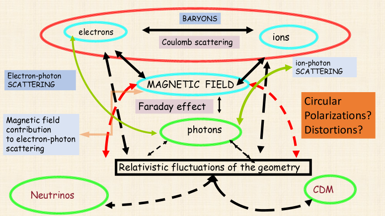
Figure 1: The effects of magnetic random fields on the pre-decoupling plasma for temperatures much smaller than the electron mass.

In Fig. 1 the direct effects of the magnetic fields have been indicated with full (double) arrows while the indirect effects have been denoted by dashed arrows. The ellipse at the top of the picture reminds that, prior to decoupling, the electrons and ions are interacting strongly via Coulomb scattering. In some cases this observation justifies the treatment of the electron-ion fluid as a single effective species often dubbed as the baryon fluid. One of the most notable exceptions to the previous statement is represented by the Faraday effect (i.e. the rotation of the polarization plane of the CMB) and more generally by all the phenomena where the magnetic field directly affects the propagation of high-frequency electromagnetic disturbances in the plasma.

Even if photons are not electrically charged, magnetic random fields have a direct effect on their evolution (as indicated in Fig. 1). This apparently counterintuitive phenomenon occurs since, prior to decoupling, photons scatter electrons and ions (or, for short, baryons). The electron-ion-photon system is, to some extent, a unique physical entity whose evolution equations are directly modified by the magnetic random fields, at least in the low-frequency branch of the spectrum of plasma excitations.

As the dashed lines of Fig. 1 suggest, the magnetic random fields interact indirectly with all the neutral species of the plasma (i.e. neutrinos, cold dark matter particles and of course photons). The neutral species actually appear in the evolution equations of the cosmological perturbations which are also affected by the presence of random magnetic fields. In particular, through the Hamiltonian and momentum constraints, the magnetic random fields modify the dynamics of the relativistic fluctuations of the geometry without affecting the evolution of the background. These two constraints determine, respectively, the initial conditions of the density contrasts and of the peculiar velocities for all species of the plasma (both charged and neutral). As a consequence the normal modes of the system are also modified and this occurrence entails, ultimately, different sets of large-scale initial conditions of the Einstein-Boltzmann hierarchy. All together the direct and indirect effects of the magnetic random fields will then determine the final values of the temperature and polarization anisotropies of the microwave background.

The layout of the paper is, in short the following. In section 2 the physical scales of the pre-decoupling plasma will be introduced together with the main ingredients of the concordance paradigm. The contribution of the magnetic fields to the electron-photon scattering will be analyzed in the second part of the section which will be concluded by a discussion of the distortions of the microwave background spectrum.

The evolution equations of the various species that interact strongly with the magnetic field (i.e. electrons and ions and, ultimately, baryons) will be discussed in section 3. After addressing the evolution of the weakly interacting species (i.e. neutrinos and cold dark matter particles), we shall tackle the magnetized scalar, vector and tensor modes of the geometry. By introducing the distinction between regular and divergent modes, the initial conditions of the Einstein-Boltzmann hierarchy will be specifically studied in terms of the normal mode of the system.

In section 4 we shall discuss some of the bounds on the magnetic fields derived in the past decade or so from the observed temperature and polarization anisotropies. We shall also illustrate the main distortions produced by magnetic random fields. The corresponding shapes of the magnetized temperature and polarization anisotropies will be briefly described by focussing on the current observables (i.e. the temperature autocorrelations, the polarization autocorrelations and the temperature-polarization cross-correlations).

Section 5 will be devoted to the analysis of the Faraday effect under different approximations and to the scaling properties of the polarization anisotropies. In section 6 we shall discuss the effects of the magnetic fields on the circular polarization (the so-called $V$-mode polarization). Section 7 contains some concluding remarks and some perspectives for the incoming decade. With the purpose of making this paper self-contained, some relevant technical aspects have been relegated to the appendix which could be useful for those who are also interested in the quantitative aspects of the problem.

2 The pre-decoupling plasma

Prior to photon decoupling the evolution of the space-time curvature and the relativistic fluctuations of the geometry cannot be neglected but the plasma parameter itself is at most of the order of $10^{-7}$, a value often encountered in diverse terrestrial plasmas from glow discharges to tokamaks. Since the Weyl invariance is broken by the masses of the charge carriers the evolution of the system cannot simply be reduced to its flat space-time analog. In this framework, the magnetic random fields affect the electron-photon scattering and, ultimately, the explicit form of the radiative transfer equations for the brightness perturbations.

2.1 Plasma parameters

The global neutrality of the plasma for redshifts $10^{3}<z<10^{6}$ implies that the concentration of the electrons and of the ions coincides, i.e. $n_{\mathrm{e}}=n_{\mathrm{i}}=n_{0}$ where $n_{0}=\eta_{\mathrm{b0}}n_{\gamma 0}$ and $n_{\gamma 0}$ denotes the present concentration of photons while, as usual, $\eta_{\mathrm{b}0}$ is the ratio between photon concentration and baryon concentration. Neglecting, for the moment, the expansion of the background geometry the plasma parameter [55, 56, 57] is given by:

$$g_{\mathrm{plasma}}=\frac{1}{V_{\mathrm{D}}n_{0}x_{\mathrm{e}}}=24e^{3}\sqrt{\frac{\overline{\zeta}(3)}{\pi}}\sqrt{x_{\mathrm{e}}\,\eta_{\mathrm{b}0}}=2.308\times 10^{-7}\sqrt{x_{\mathrm{e}}}\biggl{(}\frac{h_{0}^{2}\Omega_{\mathrm{b0}}}{0.02273}\biggr{)}^{1/2},$$ (2.1)

where $e$ is the electric charge and $\overline{\zeta}(3)=1.202\,...$; $x_{\mathrm{e}}$ is the ionization fraction and $\Omega_{\mathrm{b}0}$ is present critical fraction of baryons. In Eq. (2.1) $\lambda_{\mathrm{D}}$ is the Debye length and $V_{\mathrm{D}}$ is the volume of the Debye sphere:

$$\lambda_{\mathrm{D}}=\sqrt{\frac{T}{8\pi e^{2}n_{0}x_{\mathrm{e}}}},\qquad V_{\mathrm{D}}=\frac{4}{3}\pi\lambda_{\mathrm{D}}^{3},$$ (2.2)

where $T$ denotes the temperature of the plasma. Both $g_{\mathrm{plasma}}$ and its inverse (measuring the number of charge carriers within the Debye sphere) determine all the physically relevant hierarchies between the plasma parameters. Indeed, the Debye length (i.e. $\lambda_{\mathrm{D}}$) is parametrically smaller than the Coulomb mean free path (i.e. $\lambda_{\mathrm{Coul}}$) because of one power of $g_{\mathrm{plasma}}$:

$$\frac{\lambda_{\mathrm{D}}}{\lambda_{\mathrm{Coul}}}=\frac{g_{\mathrm{plasma}}}{48\pi}\ln{\Lambda_{\mathrm{C}}},\qquad\Lambda_{\mathrm{C}}=\frac{18\sqrt{2}}{g_{\mathrm{plasma}}},$$ (2.3)

where $\ln{\Lambda}_{\mathrm{C}}$ defines the Coulomb logarithm. In similar terms the plasma frequency of the electrons (i.e. $\omega_{\mathrm{pe}}$) is much larger than the collision frequency that is related, in its turn, to the Coulomb rate of interactions (i.e. $\Gamma_{\mathrm{Coul}}$):

$$\frac{\Gamma_{\mathrm{Coul}}}{\omega_{\mathrm{pe}}}=\frac{\ln{\Lambda_{\mathrm{C}}}}{24\sqrt{2}\pi}g_{\mathrm{plasma}},\qquad\omega_{\mathrm{pe}}=\sqrt{\frac{4\pi n_{0}x_{\mathrm{e}}}{m_{\mathrm{e}}}}.$$ (2.4)

Since the conductivity $\sigma$ depends both on the plasma frequency and on the Coulomb rate [55, 57] we can use Eq. (2.4) and express $\sigma$ in terms of the plasma parameter:

$$\sigma=\frac{\omega_{\mathrm{pe}}^{2}}{4\pi\Gamma_{\mathrm{Coul}}}=\frac{6\sqrt{2}}{\ln{\Lambda_{\mathrm{C}}}}\frac{\omega_{\mathrm{pe}}}{g_{\mathrm{plasma}}}.$$ (2.5)

The three hierarchies discussed in Eqs. (2.3), (2.4) and (2.5) should be supplemented by a fourth one, not directly related to the plasma parameter. The Hubble radius $r_{\mathrm{H}}=H^{-1}$ around equality exceeds (roughly by 20 orders of magnitude) the Debye length at the corresponding epoch. At the same reference time, magnetic fields can be present only over sufficiently large scales $L>L_{\sigma}$ where $L_{\sigma}$ is the magnetic diffusivity scale

$$L_{\sigma}\simeq(4\pi\sigma H_{\mathrm{eq}})^{-1},\qquad\sigma=\frac{T}{e^{2}\ln{\Lambda_{\mathrm{C}}}}\biggl{(}\frac{T}{m_{\mathrm{e}}}\biggr{)}^{1/2}.$$ (2.6)

In these conditions the Larmor radius prior to matter-radiation equality is always much smaller than the range of variation of the magnetic field, i.e.

$$r_{\mathrm{Be}}\ll L\simeq r_{\mathrm{H}},\qquad r_{\mathrm{Be}}=\frac{v_{\perp}}{\omega_{\mathrm{Be}}},\qquad v_{\perp}\simeq v_{\mathrm{th}},$$ (2.7)

where $v_{\mathrm{th}}\simeq\sqrt{3T/m_{\mathrm{e}}}$ and $\omega_{\mathrm{Be}}$ is the Larmor frequency. Equation (2.7) is the starting point for the so-called guiding center approximation [60, 61] which accounts for the motion of charged particles in the magnetized plasma and will be relevant when discussing the effects of magnetic random fields on the electron-photon scattering.

2.2 Gravitating plasmas

Denoting by $\ell_{P}=\sqrt{8\pi G}$ the Planck length and by $T_{\mu}^{\nu}$ the (covariantly conserved) total energy-momentum tensor of the plasma, the Einstein equations shall be written as:

$$R_{\mu}^{\nu}-\frac{1}{2}\delta_{\mu}^{\nu}\,R=\ell_{P}^{2}\,T_{\mu}^{\nu},\qquad\nabla_{\mu}T^{\mu\nu}=0,$$ (2.8)

where $R_{\mu\nu}$ is the Ricci tensor, $R$ is the Ricci scalar. The total energy-momentum tensor $T^{\mu\nu}$ is the sum of all the individual energy-momentum tensors of the various species of the plasma:

$$T^{\mu\nu}=T^{\mu\nu}_{(\mathrm{e})}+T^{\mu\nu}_{(\mathrm{i})}+T^{\mu\nu}_{(\nu)}+T^{\mu\nu}_{(\gamma)}+T^{\mu\nu}_{(\mathrm{c})}+T^{\mu\nu}_{(\Lambda)}+T^{\mu\nu}_{(\mathrm{EM})}.$$ (2.9)

In Eq. (2.9) the subscripts denote, respectively, the contributions of electrons, ions, neutrinos, photons, cold dark matter (CDM) particles, dark energy and electromagnetic fields. Since the electrons, the ions and the cold dark matter particles are all pressureless, their associated energy-momentum tensor becomes:

$$T^{\alpha\beta}_{(\mathrm{e})}=\rho_{\mathrm{e}}\,u_{(\mathrm{e})}^{\alpha}u_{(\mathrm{e})}^{\beta},\qquad T^{\alpha\beta}_{(\mathrm{i})}=\rho_{\mathrm{i}}\,u_{(\mathrm{i})}^{\alpha}u_{(\mathrm{i})}^{\beta},\qquad T^{\alpha\beta}_{(\mathrm{c})}=\rho_{\mathrm{c}}\,u_{(\mathrm{c})}^{\alpha}u_{(\mathrm{c})}^{\beta}.$$ (2.10)

The neutrinos are massless in the concordance paradigm and energy-momentum tensor will have exactly the same form as the one of the photons:

$$T^{\alpha\beta}_{(\nu)}=\frac{4}{3}\rho_{\nu}\,u^{\alpha}_{(\nu)}u^{(\beta)}_{(\nu)}-\frac{\rho_{\nu}}{3}g^{\alpha\beta},\qquad T^{\alpha\beta}_{(\gamma)}=\frac{4}{3}\rho_{\gamma}\,u^{\alpha}_{(\gamma)}u^{(\beta)}_{(\gamma)}-\frac{\rho_{\gamma}}{3}g^{\alpha\beta}.$$ (2.11)

In Eq. (2.11) the energy-momentum tensor of the neutrinos should also contain a contribution from the anisotropic stress which is fully inhomogeneous and only affects the evolution of the relativistic fluctuations of the geometry. Finally the energy-momentum tensors of the electromagnetic field and of the dark energy component is given by:

$$T_{(\mathrm{EM})}^{\alpha\beta}=\frac{1}{4\pi}\biggl{[}-F^{\alpha\mu}F^{\beta}_{\mu}+\frac{1}{4}g^{\alpha\beta}F_{\mu\nu}F^{\mu\nu}\biggr{]},\qquad T^{\alpha\beta}_{\Lambda}=\rho_{\Lambda}g^{\alpha\beta},$$ (2.12)

where $F_{\mu\nu}$ is the Maxwell field strength. In Eq. (2.12) the dark energy component is parametrized in terms of a cosmological constant, as it happens in the context of the concordance paradigm. Thus the relativistic fluctuations of the dark energy component are absent. As soon as we deviate from this choice the dark energy supports its own fluctuations.

The evolution equations of the background follow directly by writing Eq. (2.8) in the metric of Eqs. (1.5) and they are:

$$3{\mathcal{H}}^{2}=\ell_{P}^{2}a^{2}\rho_{\mathrm{t}},\qquad 2({\mathcal{H}}^{2}-{\mathcal{H}}^{\prime})=\ell_{P}^{2}a^{2}(p_{\mathrm{t}}+\rho_{\mathrm{t}}),$$ (2.13)

$$\rho_{\mathrm{t}}^{\prime}+3{\mathcal{H}}(\rho_{\mathrm{t}}+p_{\mathrm{t}})=0,\qquad{\mathcal{H}}=\frac{a^{\prime}}{a},$$ (2.14)

where the prime denotes a derivation with respect to the conformal time coordinate $\tau$; as usual the relation of ${\mathcal{H}}$ to the standard Hubble rate is given by ${\mathcal{H}}=aH$ where $H=\dot{a}/a$; note that the overdot denotes a derivation with respect to the cosmic time coordinate $t$. Moreover, by definition of cosmic time coordinate, we also have $dt=a(\tau)\,d\tau$. In the paper the derivation with respect to $\tau$ has been also denoted by $\partial_{\tau}$ in all the situations where the use of the prime would lead to potential ambiguities. The total energy density and the total pressure appearing in Eqs. (2.13) and (2.14) are

$$\rho_{\mathrm{t}}=\rho_{\mathrm{e}}+\rho_{\mathrm{i}}+\rho_{\gamma}+\rho_{\nu}+\rho_{\mathrm{c}}+\rho_{\Lambda},\qquad p_{\mathrm{t}}=\frac{\rho_{\gamma}}{3}+\frac{\rho_{\nu}}{3}-\rho_{\Lambda}.$$ (2.15)

The energy density of the magnetic fields is negligible in comparison with the energy density of the plasma but it is not negligible in comparison with the plasma inhomogeneities. By definition, the isotropic random fields of Eq. (1.6) have vanishing mean (see appendix A).

2.2.1 Evolution of the electromagnetic fields in curved space

The evolution of the electromagnetic fields can be summarized in terms of the following pair of generally covariant equations:

$$\nabla_{\mu}F^{\mu\nu}=4\pi j^{\nu},\qquad\nabla_{\mu}\widetilde{F}^{\mu\nu}=0,\qquad\nabla_{\mu}j^{\mu}=0,$$ (2.16)

where $\widetilde{F}^{\mu\nu}$ is the dual field strength, $j^{\nu}$ denotes the (covariantly conserved) total current of the plasma. Equations (2.16) do not change their form under a Weyl rescaling either when the total current vanishes or whenever the sources transform in an appropriate manner. We remind here that a Weyl rescaling of the four-dimensional metric corresponds to the transformation $G_{\mu\nu}\to g_{\mu\nu}=q(x)\,G_{\mu\nu}$ (where $x=(\vec{x},\tau)$ is a generic space-time coordinate). Under a Weyl rescaling the field strength and its dual transform, respectively, as $F^{\mu\nu}={\mathcal{F}}^{\mu\nu}/q^{2}(x)$ and as $\widetilde{F}^{\mu\nu}=\widetilde{{\mathcal{F}}}^{\mu\nu}/q^{2}(x)$. For instance, in the case of an Ohmic conductor with massless charge carriers the total current can be written as $j^{\nu}=\sigma(x)F^{\nu\alpha}\,u_{\alpha}$ where $\sigma(x)$ is the conductivity and Eq. (2.16) becomes

$$\partial_{\mu}\biggl{[}\sqrt{-g}\,F^{\mu\nu}\biggl{]}=4\pi\sqrt{-g}\,\sigma(x)\,F^{\nu\alpha}\,u_{\alpha},\qquad\partial_{\mu}(\sqrt{-g}\,\tilde{F}^{\mu\nu})=0,$$ (2.17)

together with the supplementary condition $g^{\alpha\beta}\,u_{\alpha}\,u_{\beta}=1$. The gravitating plasma for temperatures smaller than the MeV is not an Ohmic conductor. Since the masses of the charge carriers dominate against the (approximate) temperature of the plasma, the Weyl invariance is not preserved by the total current which is due to electrons and ions

$$j^{\mu}=e\,\widetilde{n}_{\mathrm{i}}u^{\mu}_{(\mathrm{i})}-e\,\widetilde{n}_{\mathrm{e}}u^{\mu}_{(\mathrm{e})},\qquad g_{\mu\nu}\,u^{\mu}_{(\mathrm{e})}\,u^{\nu}_{(\mathrm{e})}=1,\qquad g_{\mu\nu}\,u^{\mu}_{(\mathrm{i})}\,u^{\nu}_{(\mathrm{i})}=1,$$ (2.18)

where $e$ denotes the electric charge while $\widetilde{n}_{\mathrm{e}}$ and $\widetilde{n}_{\mathrm{i}}$ are the physical concentrations of the electrons and of the ions.

In a conformally flat background geometry the components of the electromagnetic field strengths expressed in terms of the physical electric and magnetic fields are given by $F_{0i}=-a^{2}\,{\mathcal{E}}_{i}$ and $F_{ij}=-a^{2}\epsilon_{ijk}{\mathcal{B}}^{k}$. Equations (2.16) then imply the following form of the Maxwell equations:

$$\vec{\nabla}\cdot\vec{E}=4\pi e(n_{\mathrm{i}}-n_{\mathrm{e}}),\qquad\vec{\nabla}\cdot\vec{B}=0,$$ (2.19)

$$\vec{\nabla}\times\vec{B}=4\pi e(n_{\mathrm{i}}\,\vec{v}_{\mathrm{i}}-n_{\mathrm{e}}\,\vec{v}_{\mathrm{e}})+\partial_{\tau}\vec{E},\qquad\vec{\nabla}\times\vec{E}=-\partial_{\tau}\vec{B},$$ (2.20)

where the comoving concentrations and the comoving electromagnetic fields are defined as:

$$n_{\mathrm{i}}=a^{3}\widetilde{n}_{\mathrm{i}},\qquad n_{\mathrm{e}}=a^{3}\widetilde{n}_{\mathrm{e}},\qquad\vec{E}=a^{2}\vec{{\mathcal{E}}},\qquad\vec{B}=a^{2}\vec{{\mathcal{B}}}.$$ (2.21)

In Eq. (2.20) the peculiar velocities of the electrons and ions are defined as $u^{k}_{(\mathrm{e})}=u^{0}_{(\mathrm{e})}v_{\mathrm{e}}^{k}$ and by $u^{k}_{(\mathrm{i})}=u^{0}_{(\mathrm{i})}v_{\mathrm{i}}^{k}$ as it follows from the general expression of the four-velocity. The peculiar velocity can also be expressed as $v^{i}=P^{i}/P^{0}$ where the physical momenta are often replaced by the comoving three-momenta $\vec{q}$ defined as:

$$P^{0}=\frac{1}{a^{2}}\sqrt{m^{2}a^{2}+q^{2}},\qquad P_{0}=\sqrt{m^{2}a^{2}+q^{2}},\qquad q^{i}=a^{2}P^{i},$$ (2.22)

which also implies that $\vec{v}=\vec{q}/\sqrt{q^{2}+m^{2}a^{2}}$. In the ultrarelativistic limit $\vec{v}=\vec{q}/|\vec{q}|$ (and the evolution equations would have the same flat-space-time form). Conversely, in the non-relativistic limit, $\vec{v}=\vec{q}/(ma)$ and the Weyl invariance is broken.

2.2.2 Comoving and physical descriptions

Since Weyl invariance is broken the plasma descriptions in curved and flat space-time are in general not the same. Recalling Eqs. (2.3), (2.4) and (2.5), the plasma parameter and the Debye length can be written in terms of the physical concentration $\widetilde{n}_{0}$:

$$\widetilde{g}_{\mathrm{plasma}}=\frac{3}{4\pi\widetilde{n}_{0}\widetilde{\lambda}_{\mathrm{D}}^{3}x_{\mathrm{e}}},\qquad\widetilde{\lambda}_{\mathrm{D}}=\sqrt{\frac{\widetilde{T}}{8\pi e^{2}\widetilde{n}_{0}x_{\mathrm{e}}}},$$ (2.23)

where the tilde denotes the corresponding physical variable. For instance the physical temperature and the physical concentration are, respectively, $\widetilde{T}=T(a_{0}/a)$ and $\widetilde{n}_{0}=n_{0}(a_{0}/a)^{3}$; $T$ and $n_{0}$ denote instead the comoving variables. It follows from Eq. (2.23) that the plasma parameter has the same value in the comoving and in the physical descriptions and it is therefore invariant:

$$\widetilde{g}_{\mathrm{plasma}}=g_{\mathrm{plasma}}=\frac{3}{4\pi n_{0}\lambda_{\mathrm{D}}^{3}x_{\mathrm{e}}},\qquad\widetilde{\lambda}_{\mathrm{D}}=\lambda_{\mathrm{D}}(a/a_{0}),\qquad\lambda_{\mathrm{D}}=\sqrt{\frac{T}{8\pi e^{2}n_{0}x_{\mathrm{e}}}},$$ (2.24)

where $\lambda_{\mathrm{D}}$ and $g_{\mathrm{plasma}}$ are, respectively, the comoving Debye scale and the comoving plasma parameter.

Because of the difference between comoving and physical three-momenta in the massive limit, the plasma frequencies for electrons and ions can be expressed either in comoving or in physical terms:

$$\overline{\omega}_{\mathrm{p}X}=\sqrt{\frac{4\pi n_{\mathrm{i}}e^{2}}{m_{X}a}}\equiv\omega_{\mathrm{p}X}a,\qquad\omega_{\mathrm{p}X}=\sqrt{\frac{4\pi\tilde{n}_{X}e^{2}}{m_{X}}},$$ (2.25)

where $X=\mathrm{i},\,\mathrm{e}$ corresponds either to the electrons or to the ions; moreover $\overline{\omega}_{\mathrm{p}X}$ and $\omega_{\mathrm{p}X}$ denote respectively the comoving and the physical frequencies. With the same notations the comoving Larmor frequencies for the electrons and for the ions are instead given by:

$$\overline{\omega}_{\mathrm{B}X}=\frac{e\vec{B}\cdot\hat{n}}{m_{X}a}=\omega_{\mathrm{B}X}a,\qquad\omega_{\mathrm{B}X}=\frac{e\vec{{\mathcal{B}}}\cdot\hat{n}}{m_{X}},$$ (2.26)

where the relation between the comoving and the physical magnetic fields is given in Eq. (2.21) and $\hat{n}$ denotes the magnetic field orientation. A direct consequence of Eqs. (2.25) and (2.26) is that the explicit expression of the comoving Larmor and plasma frequencies depend on the redshift:

$$\overline{\omega}_{\mathrm{Be}}=1.7\times 10^{-2}\biggl{(}\frac{\hat{n}\cdot\vec{B}}{\mathrm{nG}}\biggr{)}(z+1)\,\mathrm{Hz},\,\,\,\overline{\omega}_{\mathrm{pe}}=0.3\,\sqrt{x_{\mathrm{e}}}\,\biggl{(}\frac{h_{0}^{2}\Omega_{\mathrm{b}0}}{0.022}\biggr{)}^{1/2}\sqrt{z+1}\,\mathrm{MHz},$$ (2.27)

$$\overline{\omega}_{\mathrm{Bi}}=9.5\times 10^{-6}\biggl{(}\frac{\hat{n}\cdot\vec{B}}{\mathrm{nG}}\biggr{)}(z+1)\,\mathrm{Hz},\,\,\,\overline{\omega}_{\mathrm{pi}}=6.6\,\sqrt{x_{\mathrm{e}}}\,\biggl{(}\frac{h_{0}^{2}\Omega_{\mathrm{b}0}}{0.022}\biggr{)}^{1/2}\sqrt{z+1}\,\mathrm{kHz}.$$ (2.28)

The use of comoving or physical descriptions depends on the convenience. For instance the bounds on the magnetic field intensity are often compiled by using a comoving description. Conversely the values of the magnetic field and of the other plasma parameter in the bottom line of

Plasma	$\widetilde{n}_{0}[m^{-3}]$	$\widetilde{T}$ [keV]	${\mathcal{B}}$[G]	$\omega_{\mathrm{pe}}$[Hz]	$\widetilde{\lambda}_{\mathrm{D}}$[m]	$\widetilde{n}_{0}x_{e}\widetilde{\lambda}_{D}^{3}$	$\widetilde{\Gamma}_{\mathrm{Coul}}$[Hz]
tokamak	$10^{20}$	$10$	$10^{5}$	$10^{11}$	$10^{-5}$	$10^{7}$	$10^{4}$
glow discharge	$10^{20}$	$10^{-3}$	$10^{3}$	$6\times 10^{11}$	$10^{-7}$	$100$	$10^{10}$
solar corona	$10^{12}$	$10^{-1}$	$10$	$10^{7}$	$10^{-2}$	$10^{8}$	$10^{-1}$
pre-decoupling	$10^{9}$	$10^{-3}$	$<10^{-2}$	$10^{5}\,\sqrt{x_{e}}$	$10^{-2}$	$10^{6}/\sqrt{x_{e}}$	$10^{-2}x_{e}$

Table 2: Plasma parameters of some common physical system compared with the pre-decoupling plasma; $x_{e}$ denotes the ionization fraction.

Tab. 2 are computed for the typical reference temperature of the eV roughly corresponding to the equality between matter and radiation occurring at a redshift:

$$1+z_{\mathrm{eq}}=\frac{a_{0}}{a_{\mathrm{eq}}}=\frac{h_{0}^{2}\Omega_{\mathrm{M}0}}{h_{0}^{2}\Omega_{\mathrm{R}0}}=3228.91\biggl{(}\frac{h_{0}^{2}\Omega_{\mathrm{M}0}}{0.134}\biggr{)}.$$ (2.29)

For comparison photon decoupling takes place at a typical redshift $z_{*}={\mathcal{O}}(1100)$ (i.e. between $1080$ and $1110$). In Tab. 2 we also illustrate the same plasma parameters for other examples of highly ionized plasmas. Note that the number of charged carriers within the Debye sphere is grossly the same for the pre-decoupling plasma, for the solar corona and for a tokamak (see second column from the right in Tab. 2). Similar comparisons can be developed in the case of the other plasma parameters by always reminding, as emphasized in Eqs. (2.3)–(2.5) that the various hierarchies are controlled either by $g_{\mathrm{plasma}}$ or by its inverse.

2.2.3 The approximate temperature of the plasma

The evolution of the approximate temperature of the plasma depends on $g_{\mathrm{plasma}}$. Indeed when the plasma contains an equal number of positively and negatively charged species in a radiation background its total energy density and pressure are:

$$\overline{\rho}_{\mathrm{tot}}=\rho_{+}+\rho_{-}+\rho_{r},\qquad\overline{p}_{\mathrm{tot}}=p_{+}+p_{-}+p_{r}.$$ (2.30)

As long as the physical temperatures of the charged species exceed the corresponding masses (i.e. $\widetilde{T}_{\pm}\gg m_{\pm}$), the temperatures $\widetilde{T}_{+}$ and $\widetilde{T}_{-}$ approximately coincide with $\widetilde{T}_{r}$ which is, by definition, the temperature of the radiation, i.e. $\widetilde{T}_{+}\simeq\widetilde{T}_{-}\simeq\widetilde{T}_{r}$. In the opposite case (i.e. for $\widetilde{T}_{\pm}<m_{\pm}$) the evolution of the various temperatures depends on $g_{\mathrm{plasma}}$. From Eqs. (2.30) the first principle of the thermodynamics and the adiabaticity of the evolution imply:

$$d\biggl{\{}V_{H}\,\biggl{[}(\widetilde{n}_{+}m_{+}+\widetilde{n}_{-}m_{-})+\frac{3}{2}\biggl{(}\widetilde{n}_{+}\widetilde{T}_{+}+\widetilde{n}_{-}\widetilde{T}_{-}\biggr{)}+\rho_{r}\biggr{]}\biggr{\}}+\biggl{(}\widetilde{n}_{+}\widetilde{T}_{+}+\widetilde{n}_{-}\widetilde{T}_{-}+p_{r}\biggr{)}dV_{H}=0,$$ (2.31)

where $V_{H}(a)=(4\pi/3)H_{*}^{-3}a^{3}$ is the fiducial Hubble volume. Since the plasma is globally neutral (i.e. $\widetilde{n}_{+}=\widetilde{n}_{-}=\widetilde{n}_{0}$), Eq. (2.31) can also be expressed as:

$$d[a^{2}(\widetilde{T}_{+}+\widetilde{T}_{-})]+a\,\gamma\,d(a\widetilde{T}_{r})=0,\qquad\gamma=\frac{2s}{n_{0}},$$ (2.32)

where, besides the comoving concentration (i.e. $n_{0}=a^{3}\,\widetilde{n}_{0}$) we introduced the comoving entropy density $s=a^{3}\,\widetilde{s}$ (with $\widetilde{s}=2\pi^{2}{\mathcal{N}}_{\mathrm{th}}\widetilde{T}_{r}^{3}/45$). The physical initial conditions stipulate that $\widetilde{T}_{+}\simeq\widetilde{T}_{-}\simeq\widetilde{T}_{r}$ with the result that, thanks to Eq. (2.32), the common temperature of the different species scales as:

$$\widetilde{T}\simeq a^{-\frac{4+\gamma}{2+\gamma}},\qquad\gamma=\frac{4\pi^{4}}{45\,\overline{\zeta}(3)}\,\biggl{(}\frac{n_{r}}{n_{0}}\biggr{)}=\frac{16}{5}(2\pi)^{3}\,{\mathcal{N}}_{\mathrm{th}}\,\biggl{(}\frac{e^{3}}{g_{\mathrm{plasma}}}\biggr{)}^{2}.$$ (2.33)

where $\overline{\zeta}(3)$ has been already introduced after Eq. (2.1) and $n_{r}=a^{3}\widetilde{n}_{r}$; note that $\widetilde{n}_{r}={\mathcal{N}}_{\mathrm{th}}\,\widetilde{T}_{r}^{3}\,\overline{\zeta}(3)/\pi^{2}$. If $n_{r}\ll n_{0}$, the temperature scales, approximately, as $a^{-2}$ in the opposite case (i.e. $n_{r}\gg n_{0}$) the effective temperature evolves, to first order in $1/\gamma$, as $a^{-1}$. Since prior to decoupling $g_{\mathrm{plasma}}\ll 1$ and $\gamma\propto g_{\mathrm{plasma}}^{-2}$, we are exactly in the limit $\gamma\gg 1$.

2.3 Relativistic fluctuations of the geometry

The relativistic fluctuations of the conformally flat background of Eq. (1.5) (i.e. $g_{\mu\nu}(\vec{x},\tau)=\overline{g}_{\mu\nu}(\tau)+\delta g_{\mu\nu}(\vec{x},\tau)$) can be separated into scalar, vector and tensor modes as originally suggested by Lifshitz [46, 64]:

$$\delta g_{\mu\nu}(\vec{x},\tau)=\delta_{\mathrm{s}}g_{\mu\nu}(\vec{x},\tau)+\delta_{\mathrm{v}}g_{\mu\nu}(\vec{x},\tau)+\delta_{\mathrm{t}}g_{\mu\nu}(\vec{x},\tau),$$ (2.34)

where $\delta_{\mathrm{s}}$, $\delta_{\mathrm{v}}$ and $\delta_{\mathrm{t}}$ denote the inhomogeneity preserving, separately, the scalar, vector and tensor nature of the corresponding fluctuations. Magnetic random fields affect the evolution of the relativistic fluctuations of the geometry and, in particular, of the large-scale curvature inhomogeneities. Some relevant aspects of this well known problem will now be swiftly outlined.

2.3.1 Scalar, vector and tensor modes

The scalar modes of the geometry are parametrized in terms of four independent functions $\psi(\vec{x},\tau)$, $\phi(\vec{x},\tau)$, $F(\vec{x},\tau)$ and $G(\vec{x},\tau)$:

$$\delta_{\mathrm{s}}g_{00}(\vec{x},\tau)=2a^{2}(\tau)\phi(\vec{x},\tau),\qquad\delta_{\mathrm{s}}g_{0i}(\vec{x},\tau)=-a^{2}(\tau)\partial_{i}F(\vec{x},\tau),$$

$$\delta_{\mathrm{s}}g_{ij}(\vec{x},\tau)=2a^{2}(\tau)[\psi(\vec{x},\tau)\delta_{ij}-\partial_{i}\partial_{j}G(\vec{x},\tau)],$$ (2.35)

The vector modes are described by two independent vectors $Q_{i}(\vec{x},\tau)$ and $W_{i}(\vec{x},\tau)$:

$$\delta_{\mathrm{v}}g_{0i}(\vec{x},\tau)=-a^{2}Q_{i}(\vec{x},\tau),\qquad\delta_{\mathrm{v}}g_{ij}(\vec{x},\tau)=a^{2}\biggl{[}\partial_{i}W_{j}(\vec{x},\tau)+\partial_{j}W_{i}(\vec{x},\tau)\biggr{]},$$ (2.36)

subjected to the conditions $\partial_{i}Q^{i}=0$ and $\partial_{i}W^{i}=0$. Finally the tensor modes of the geometry are parametrized in terms of a rank-two tensor in three spatial dimensions, i.e.

$$\delta_{t}g_{ij}(\vec{x},\tau)=-a^{2}h_{ij}(\vec{x},\tau),\qquad\partial_{i}h^{i}_{j}(\vec{x},\tau)=h_{i}^{i}(\vec{x},\tau)=0.$$ (2.37)

For an infinitesimal coordinate shift $x^{\mu}\to\widetilde{x}^{\mu}=x^{\mu}+\epsilon^{\mu}$ the scalar and vector modes of Eqs. (2.35) and (2.36) transform according to the Lie derivative in the direction $\epsilon^{\mu}=(\epsilon^{0},\,\epsilon^{i})$. The scalar fluctuations in the tilded coordinate system read

$$\phi\to\widetilde{\phi}=\phi-{\cal H}\epsilon_{0}-\epsilon_{0}^{\prime},\qquad\psi\to\widetilde{\psi}=\psi+{\cal H}\epsilon_{0},$$ (2.38)

$$F\to\widetilde{F}=F+\epsilon_{0}-\epsilon^{\prime},\qquad G\to\widetilde{G}=G-\epsilon.$$ (2.39)

For the sake of simplicity in Eq. (2.39) the arguments of the various functions have been neglected and will be omitted hereunder unless strictly necessary. Following the same notations, the vector modes transform as:

$$Q_{i}\to\widetilde{Q}_{i}=Q_{i}-\zeta_{i}^{\prime},\qquad W_{i}\to\widetilde{W}_{i}=W_{i}+\zeta_{i}.$$ (2.40)

In the case of the vector modes the gauge choices are extremely limited and while a convenient gauge is $Q_{i}=0$, there are two unambiguous gauge-invariant variables that arise when combining the fluctuations of the metric with the vector fluctuations of the sources (see Eq. (3.98) and discussion thereafter). In the scalar case the possible gauge choices are more numerous than for the vector modes. For instance if $G$ and $F$ are set to zero in Eq. (2.35) the gauge freedom is completely fixed (see Eq. (2.39)) and this choice pins down the conformally Newtonian gauge [65] where the longitudinal fluctuations of the metric read, in Fourier space,

$$\delta_{\mathrm{s}}\,g_{00}(k,\tau)=2a^{2}\,\phi(k,\tau),\qquad\delta_{\mathrm{s}}g_{ij}=2a^{2}\psi(k,\tau)\delta_{ij}.$$ (2.41)

By instead setting $\phi$ and $F$ to zero we recover the standard choice of the synchronous coordinate system [66, 67] where the metric fluctuations can be written, in Fourier space, as [67]

$$\delta_{\rm s}g_{ij}(k,\tau)=a^{2}(\tau)\biggl{[}\hat{k}_{i}\hat{k}_{j}h(k,\tau)+6\xi(k,\tau)\biggl{(}\hat{k}_{i}\hat{k}_{j}-\frac{1}{3}\delta_{ij}\biggr{)}\biggr{]},$$ (2.42)

where, as usual, $\hat{k}_{i}=k_{i}/|\vec{k}|$. Finally the third convenient choice for the analyses of large-scale magnetism is the off-diagonal (or uniform curvature) gauge demanding that $\psi=F=0$ in Eq. (2.35) [68, 69, 70].

2.3.2 Gauge-invariant normal modes of the system

In the tensor case the normal modes coincide, up to a trivial field redefinition involving the scale factor, with the metric fluctuation introduced in Eq. (2.37). The evolution of the tensor modes breaks Weyl invariance and it has been derived well before the formulation of the inflationary scenario [71, 72]:

$$h_{ij}^{\prime\prime}+2{\mathcal{H}}h_{ij}^{\prime}-\nabla^{2}h_{ij}=0.$$ (2.43)

In the scalar case the normal modes are the curvature perturbations on comoving orthogonal hypersurfaces , conventionally denoted by ${\mathcal{R}}$. In the comoving orthogonal gauge the fluctuations of the spatial curvature correspond to ${\mathcal{R}}$, i.e. $\delta_{\mathrm{s}}^{(3)}R=-(4/a^{2})\nabla^{2}{\mathcal{R}}$. When the background is dominated by an irrotational relativistic fluid the evolution of ${\mathcal{R}}$ is:

$${\mathcal{R}}^{\prime\prime}+2\frac{z_{\mathrm{t}}^{\prime}}{z_{\mathrm{t}}}{\mathcal{R}}^{\prime}-c_{\mathrm{st}}^{2}\nabla^{2}{\mathcal{R}}=0,\qquad z_{\mathrm{t}}=\frac{a^{2}\sqrt{\rho_{\mathrm{t}}+p_{\mathrm{t}}}}{{\mathcal{H}}\,c_{\mathrm{st}}},$$ (2.44)

where $c_{\mathrm{st}}^{2}=p_{\mathrm{t}}^{\prime}/\rho_{\mathrm{t}}^{\prime}$; note that $\rho_{\mathrm{t}}$ and $p_{\mathrm{t}}$ enter directly the background equations (2.13) and (2.14). The variable of Eqs. (2.44) and (2.46) has been first discussed by Lukash [73] (see also [74, 75]) when analyzing the quantum excitations of an irrotational and relativistic fluid. The canonical normal mode identified in Ref. [73] is invariant under infinitesimal coordinate transformations as required in the context of the Bardeen formalism [65]. If the background is instead dominated by a single scalar field $\varphi$ the analog of Eq. (2.44) can be written as:

$${\mathcal{R}}^{\prime\prime}+2\frac{z_{\varphi}^{\prime}}{z_{\varphi}}{\mathcal{R}}^{\prime}-\nabla^{2}{\mathcal{R}}=0,\qquad z_{\varphi}=\frac{a\varphi^{\prime}}{\mathcal{H}}.$$ (2.45)

Equation (2.45) has been derived in the case of scalar field matter in Refs. [76] and [77]. These analyses follow the same logic of [73] (see Eq. (2.44)). The normal modes of Eqs. (2.44) and (2.45) coincide with the (rescaled) curvature perturbations on comoving orthogonal hypersurfaces [78, 79]. Once the curvature perturbations are computed (either from Eq. (2.44) or from Eq. (2.45)) the metric fluctuations can be easily derived in a specific gauge. Since ${\mathcal{R}}$ is gauge-invariant, its value is, by definition, the same in any coordinate system even if its expression changes from one gauge to the other. For instance, in the synchronous (i.e. Eq. (2.42)) and longitudinal (i.e. Eq. (2.41)) gauges the expression of ${\mathcal{R}}$ is, respectively

$${\mathcal{R}}^{(S)}=\frac{{\mathcal{H}}}{{\mathcal{H}}^{2}-{\mathcal{H}}^{\prime}}\xi^{\prime}+\xi,\qquad{\mathcal{R}}^{(L)}=-\psi-\frac{{\mathcal{H}}({\mathcal{H}}\phi+\psi^{\prime})}{{\mathcal{H}}^{2}-{\mathcal{H}}^{\prime}}.$$ (2.46)

Even if the expressions ${\mathcal{R}}^{(L)}$ and ${\mathcal{R}}^{(S)}$ of Eq. (2.46) are formally different, the invariance under infinitesimal coordinate transformations implies that the values of ${\mathcal{R}}$ computed in different gauges must coincide, i.e. ${\mathcal{R}}^{(S)}={\mathcal{R}}^{(L)}={\mathcal{R}}$.

2.4 The concordance paradigm

The $\Lambda$CDM paradigm is just a useful compromise between the available data, the standard cosmological model and the number of ascertainable parameters. The turning point shaping the present form of the $\Lambda$CDM scenario has been the WMAP program with the first analysis of the cross-correlation between the temperature and the polarization anisotropies [81, 82]. The position of the first Doppler peak in the temperature autocorrelations and the location of the first anti-correlation peak of the polarization implied that the source of large-scale inhomogeneities accounting for the CMB anisotropies had to be adiabatic and Gaussian fluctuations of the spatial curvature [81, 82]. This evidence, subsequently confirmed by the following data releases of the WMAP experiment [83, 84, 85] and by the Planck collaboration [86, 87, 88, 89, 90], justifies and motivates the current formulation of the concordance paradigm where the dominant source of large-scale inhomogeneity are the adiabatic curvature perturbations.

2.4.1 The pivotal parameters

The $\Lambda$CDM paradigm is formulated in terms of six pivotal parameters that are customarily chosen as follows: i) the present critical fraction of baryonic matter [i.e. $\Omega_{b0}=\rho_{b0}/\rho_{crit}={\mathcal{O}}(0.048)$]; ii) the present critical fraction of CDM particles, [i.e. $\Omega_{c0}=\rho_{c0}/\rho_{crit}={\mathcal{O}}(0.26)$]; iii) the present critical fraction of dark energy, [i.e. $\Omega_{\Lambda}=\rho_{\Lambda}/\rho_{crit}={\mathcal{O}}(0.7)$]; iv) the indetermination on the Hubble rate [i.e. $h_{0}={\mathcal{O}}(0.7)$]; v) the spectral index scalar inhomogeneities [i.e. $n_{\mathrm{s}}={\mathcal{O}}(0.967)$]; vi) the optical depth at reionization [i.e. $\epsilon_{re}={\mathcal{O}}(0.07)$].

The parameters of the $\Lambda$CDM paradigm can be inferred either by considering a single class of data (e.g. microwave background observations) or by requiring the consistency of the scenario with the three observational data sets represented, generally speaking, by the temperature and polarization anisotropies of the microwave background, by the extended galaxy surveys (see e.g. [91, 92]) and by the supernova observations (see e.g. [93, 94]). There have been 5 different releases of the WMAP data [81, 82, 83, 84, 85] corresponding to one, three, five, seven and nine years of integrated observations. The various releases led to compatible (but slightly different) determinations of the pivotal parameters of the $\Lambda$CDM paradigm. A similar comment holds for the two releases of the Planck collaboration [86, 87, 88, 89, 90]. Various terrestrial observations of the temperature and polarization anisotropies have been reported (see e.g. [95, 96, 97, 98, 99, 100, 101, 102]) and they have been sometimes used to infer specific limits on magnetic random fields.

Data	WMAP5	WMAP7	WMAP9	PLANCK
$\Omega_{b0}$	$0.0441\pm 0.0030$	$0.0449\pm 0.0028$	$0.0463\pm 0.0024$	$0.0486\pm 0.0010$
$\Omega_{c0}$	$0.214\pm 0.027$	$0.222\pm 0.026$	$0.233\pm 0.023$	$0.2589\pm 0.0057$
$\Omega_{\Lambda}$	$0.742\pm 0.030$	$0.734\pm 0.029$	$0.721\pm 0.025$	$0.6911\pm 0.0062$
$H_{0}$	$71.9^{+2.6}_{-2.7}$	$71.0\pm 2.5$	$70.0\pm 2.2$	$67.74\pm 0.46$
$n_{\mathrm{s}}$	$0.963^{+0.014}_{-0.015}$	$0.963\pm 0.014$	$0.972\pm 0.013$	$0.9667\pm 0.0040$
$\epsilon_{re}$	$0.087\pm 0.017$	$0.088\pm 0.015$	$0.089\pm 0.014$	$0.066\pm 0.012$
$r_{T}$	$<0.43$	$<0.36$	$<0.34$	$<0.1$

Table 3: The six pivotal parameters of $\Lambda$CDM scenario. The best fits of the WMAP5, WMAP7 and WMAP9 data alone are compared with the Planck fiducial set of parameters.

In Tab. 3 the determination of the various $\Lambda$CDM parameters of the last three data releases of the WMAP experiment is compared with the Planck fiducial set of parameters. In the last line, for reference, the limits on the tensor-to-scalar ratio have been illustrated.

2.4.2 Neutrinos, photons and baryons

The minimal $\Lambda$CDM paradigm (sometimes referred to as the vanilla $\Lambda$CDM scenario) assumes that the neutrinos are strictly massless and the tensor modes of the geometry are absent. The radiation component can therefore be directly computed from the photon and from the neutrino temperatures. The energy density of a massless neutrino background is today

$$\rho_{\nu 0}=\frac{21}{8}\biggl{(}\frac{4}{11}\biggr{)}^{4/3}\rho_{\gamma 0},\qquad h_{0}^{2}\Omega_{\nu 0}=1.68\times 10^{-5},$$ (2.47)

while the contribution of the photons is given by $h_{0}^{2}\Omega_{\gamma 0}=2.47\times 10^{-5}$. The factor $(4/11)^{4/3}$ stems from the relative reduction of the neutrino (kinetic) temperature (in comparison with the photon temperature) after weak interactions fall out of thermal equilibrium (see e.g. [103, 104] and also appendix A of Ref. [105]). The photon fraction in the radiation plasma (i.e $R_{\gamma}=\rho_{\gamma}/\rho_{R}$) and the corresponding neutrino fraction (i.e. $R_{\nu}=\rho_{\nu}/\rho_{R}$) obey, by definition, $R_{\gamma}=1-R_{\nu}$ and $R_{\nu}$ is:

$$R_{\nu}=\frac{\rho_{\nu}}{\rho_{\gamma}+\rho_{\nu}}=\frac{3\times(7/8)\times(4/11)^{4/3}}{1+3\times(7/8)\times(4/11)^{4/3}}=0.4052,$$ (2.48)

where $3$ counts the degrees of freedom associated with the massless neutrino families, $(7/8)$ arises because neutrinos follow the Fermi-Dirac statistics. The energy density of radiation in critical units is given today by:

$$h_{0}^{2}\Omega_{R0}=h_{0}^{2}\Omega_{\gamma 0}+h_{0}^{2}\Omega_{\nu 0}=4.15\times 10^{-5}.$$ (2.49)

To close the circle, the relative weight of photons and baryons depends on the redshift and it is parametrized in terms of $R_{b}(z)$:

$$R_{b}(z)=\frac{3}{4}\frac{\rho_{\mathrm{b}}}{\rho_{\gamma}}=0.664\biggl{(}\frac{h_{0}^{2}\Omega_{b0}}{0.023}\biggr{)}\biggl{(}\frac{1051}{z+1}\biggr{)},$$ (2.50)

where $z$ denotes the redshift. Note that the baryon to photon ratio determines the sound speed of the baryon-photon system and the sound horizon, namely:

$$c_{\mathrm{sb}}(\tau)=\frac{1}{\sqrt{3[1+R_{b}(\tau)]}},\qquad r_{\mathrm{s}}(\tau_{*})=\int_{0}^{\tau_{*}}d\tau c_{\mathrm{sb}}(\tau).$$ (2.51)

The value of the sound speed affects then the relative positions of the Doppler peak in the temperature autocorrelations (in the jargon the $TT$ correlations) and of the first anti-correlation peak of the temperature-polarization power spectrum (customarily referred to as the $TE$ correlations).

2.4.3 Large-scale inhomogeneities

The adiabatic scalar fluctuations are the dominant source of large-scale inhomogeneties in the $\Lambda$CDM scenario and they are customarily introduced in terms of the gauge-invariant curvature perturbation on comoving orthogonal hypersurfaces already mentioned in Eqs. (2.44), (2.45) and (2.46). The scalar random field ${\mathcal{R}}(\vec{x},\tau)$ corresponding to the curvature perturbation is described, in Fourier space, by its associated power spectrum $P_{{\mathcal{R}}}(k,\tau)$ (see Eqs. (A.4), (A.5) and (A.6) of appendix A for a specific discussion of the underlying notations).

The scalar power spectrum is customarily assigned as a power-law for typical length-scales larger than the Hubble radius at the corresponding time and well before matter-radiation equality :

$$P_{{\mathcal{R}}}(k,\tau)={\mathcal{A}}_{{\mathcal{R}}}\biggl{(}\frac{k}{k_{\mathrm{p}}}\biggr{)}^{n_{\mathrm{s}}-1},\qquad{\mathcal{A}}_{{\mathcal{R}}}={\mathcal{O}}(2.4)\times 10^{-9}\qquad k_{\mathrm{p}}=0.002\,\,\mathrm{Mpc}^{-1}.$$ (2.52)

where $n_{\mathrm{s}}$ is the scalar spectral index already introduced above and tabulated in Tab. 3 (see the fifth line from the top); ${\mathcal{A}}_{{\mathcal{R}}}$ measures the amplitude of curvature perturbations at the pivot scale $k_{\mathrm{p}}$ and its value is deduced from the overall normalization of the temperature autocorrelations. While the value of $k_{\mathrm{p}}$ is largely conventional, the choice of Eq. (2.52) corresponds to an effective harmonic $\ell_{\mathrm{eff}}\simeq 30$. In Eq. (2.52) the scale invariant limit (sometimes dubbed Harrison-Zeldovich [168, 52] limit) occurs for $n_{\mathrm{s}}\to 1$ (or $(n_{\mathrm{s}}-1)\to 0$).

For adiabatic initial conditions of the Einstein-Boltzmann hierarchy the $TT$ angular power spectrum has the celebrated first acoustic peak for $\ell_{\mathrm{d}}\simeq 220$. The first (anticorrelation) peak of the $TE$ spectra occurs instead for $\ell_{\mathrm{ac}}\simeq 3\,\ell_{\rm d}/4<\ell_{\mathrm{d}}\simeq 150$. As correctly argued already in the first data release of the WMAP experiment [81] this is the best evidence of the adiabatic nature of large-scale curvature perturbations. Recalling Eqs. (2.50) and (2.51) we have that the large-scale contribution to the temperature $TT$ correlation goes, in Fourier space, as $\cos{(kc_{\mathrm{sb}}\tau_{\mathrm{dec}})}$ where $\tau_{\mathrm{dec}}$ denotes approximately the decoupling time (see e.g. [81, 106] and also [103, 104, 105]). For the same set of adiabatic Cauchy data the $TE$ correlation oscillates, always in Fourier space, as $\sin{(2kc_{\mathrm{sb}}\tau_{\mathrm{dec}})}$. Consequently the first (compressional) peak of the temperature autocorrelation corresponds to $kc_{\mathrm{sb}}\tau_{\rm dec}\sim\pi$, while the first peak of the cross-correlation will arise for $kc_{\mathrm{sb}}\tau_{\rm dec}\sim 3\pi/4$ i.e., as anticipated, $\ell_{\mathrm{ac}}\simeq 3\,\ell_{\mathrm{d}}/4$. These analytic results can be obtained by working to first-order in the tight-coupling expansion [49, 81, 106, 107, 108].

From the position of the first anticorrelation peak it is possible to derive limits on the contribution of the magnetic random fields to the initial conditions of the Einstein-Boltzmann hierarchy [109]. The adiabatic nature of large-scale curvature inhomogeneities implies that the fluctuations of the specific entropy are either absent or strongly constrained. Non-adiabatic (or entropic) fluctuations are easily generated both in the early and in the late Universe and have been scrutinized in a number of different context [110, 111]. Magnetic random fields have been also studied in connection with the entropic fluctuations of the plasma [112] (see also section 3). Depending on the nature of the entropic solution, one of the most notable results of the Planck experiment implies the possibility of a non-adiabatic component smaller than about $2\%$ of the adiabatic component [90].

While the tensor modes of the geometry obeying Eq. (2.43) do not appear in the minimal $\Lambda$CDM paradigm, their power spectrum is customarily assigned as:

$$P_{\mathrm{T}}(k)={\mathcal{A}}_{\mathrm{T}}\biggl{(}\frac{k}{k_{\mathrm{p}}}\biggr{)}^{n_{\mathrm{T}}},\qquad{\mathcal{A}}_{\mathrm{T}}=r_{\mathrm{T}}{\mathcal{A}}_{{\mathcal{R}}},$$ (2.53)

where $n_{T}$ is the tensor spectral index and $r_{T}$ is often referred to as the tensor-to-scalar ratio (see also Eq. (A.17) of appendix A). Equation (2.53) requires the addition of two supplementary parameters: the spectral index and the amplitude. If the inflationary phase is driven by a single scalar degree of freedom and if the radiation dominance kicks in almost suddenly after inflation, the whole tensor contribution can be solely parametrized in terms of $r_{\mathrm{T}}$. The rationale for the latter statement is that $r_{\mathrm{T}}$ not only determines the tensor amplitude but also, thanks to the algebra obeyed by the slow-roll parameters, the slope of the tensor power spectrum. In Tab. 3 the upper limits on $r_{T}$ have been tabulated in the seventh line from the top. The direct measurement of $r_{T}$ can be achieved if the $B$-mode polarization is directly observed. The first detection of a $B$-mode polarization, coming from the lensing of the CMB anisotropies, has been published by the South Pole Telescope [101]. The $B$-mode polarization induced by the lensing of the CMB anisotropies is, however, qualitatively different from the $B$-mode induced by the tensor modes of the geometry.

2.5 Magnetized radiative transfer equations

The electron-photon scattering is customarily discussed without any magnetic field [113, 114]. However, prior to decoupling the photons scatter electrons (an ions) in a magnetized environment. Magnetic random fields affect the Stokes parameters as well as the evolution of the scalar, vector and tensor brightness perturbations [115] (see also [116, 117]).

2.5.1 Jones and Mueller calculus

The four Stokes parameters can either be organized in a $2\times 2$ matrix (as in Jones calculus) or in a column vector with four entries (as in the case of Mueller calculus). See Ref. [118] for an introduction to the Jones and Mueller approaches to the polarized radiative transfer equations. In what follows the polarization tensor ${\mathcal{P}}_{ij}={\mathcal{P}}_{ji}=E_{i}\,E_{j}^{*}$ shall be organized first in a $2\times 2$ matrix whose explicit form is:

$${\mathcal{P}}=\left(\matrix{I+Q&U-iV&\cr U+iV&I-Q&\cr}\right)=\left(I\,{\bf 1}+U\,\sigma_{1}+V\,\sigma_{2}+Q\,\sigma_{3}\right),$$ (2.54)

where ${\bf 1}$ denotes the identity matrix while $\sigma_{1}$, $\sigma_{2}$ and $\sigma_{3}$ are the three Pauli matrices. The problem depends on $6$ angles: i) $\Omega=(\vartheta,\varphi)$ defines the directions of the scattered photons, ii) $\Omega^{\prime}=(\vartheta^{\prime},\varphi^{\prime})$ accounts for the directions of the incident photons and iii) $\Omega^{\prime\prime}=(\alpha,\beta)$ denotes the magnetic field direction. The radial, azimuthal and polar directions of the scattered radiation are defined as:

$$\hat{r}=(\cos{\varphi}\sin{\vartheta},\,\sin{\varphi}\sin{\vartheta},\,\cos{\vartheta}),$$

$$\hat{\vartheta}=(\cos{\varphi}\cos{\vartheta},\,\sin{\varphi}\cos{\vartheta},\,-\sin{\vartheta}),\qquad\hat{\varphi}=(-\sin{\varphi},\,\cos{\varphi},\,0).$$ (2.55)

As it can be checked the orientation of the unit vectors is such that $\hat{r}\times\hat{\vartheta}=\hat{\varphi}$. The spherical polar coordinates of the incident photons are assigned as in Eq. (2.55) but the angles $(\vartheta,\varphi)$ are replaced by $(\vartheta^{\prime},\varphi^{\prime})$. In Fig. 2 the (thick) dashed line denotes the direction of $\hat{n}=(\vartheta,\varphi)$.

Figure 2: Schematic view of the relation between the coordinate system defining the scattered radiation field and the reference frame where the magnetic field is oriented along the third axis.

The direction defined by $\hat{e}_{1}$, $\hat{e}_{2}$ and $\hat{e}_{3}$ is determined by the angles $\alpha$ and $\beta$ illustrated in Fig. 2 and defined as:

$$\hat{e}_{1}=(\cos{\alpha}\cos{\beta},\,\sin{\alpha}\cos{\beta},\,-\sin{\beta}),$$

$$\hat{e}_{2}=(-\sin{\alpha},\,\cos{\alpha},\,0),\qquad\hat{e}_{3}=(\cos{\alpha}\sin{\beta},\sin{\alpha}\sin{\beta},\cos{\beta}).$$ (2.56)

With these specifications, the evolution of the matrix ${\mathcal{P}}$ can be formally written as

$$\frac{d{\mathcal{P}}}{d\tau}+\epsilon^{\prime}{\mathcal{P}}=\frac{3\epsilon^{\prime}}{8\pi}\int\,d\Omega^{\prime}\,M(\Omega,\Omega^{\prime},\Omega^{\prime\prime})\,{\mathcal{P}}(\Omega^{\prime})\,M^{\dagger}(\Omega,\Omega^{\prime},\Omega^{\prime\prime}),$$ (2.57)

where $d\Omega^{\prime}=\sin{\vartheta^{\prime}}\,d\vartheta^{\prime}\,d\varphi^{\prime}$ and the dagger in Eq. (2.57) defines, as usual, the complex conjugate of the transposed matrix. Defining the rate of electron-photon scattering $\Gamma_{\gamma\mathrm{e}}$ we have that the differential optical depth, the Thomson cross section and the classical radius of the electron are given, respectively, as

$$\epsilon^{\prime}=a\Gamma_{\gamma\mathrm{e}}=a\tilde{n}_{\mathrm{0}}x_{\mathrm{e}}\sigma_{\mathrm{e}\gamma},\qquad\sigma_{\gamma\mathrm{e}}=\frac{8}{3}\pi r_{\mathrm{e}}^{2},\qquad r_{\mathrm{e}}=\frac{e^{2}}{m_{\mathrm{e}}}.$$ (2.58)

In the differential optical depth the contribution of the ions is neglected since the mass of the ions is much larger than the mass of the electrons; we shall also follow this practice even if it is not strictly necessary. For reference the explicit components of the matrix $M(\Omega,\Omega^{\prime},\Omega^{\prime\prime})$ are separately reported in Eqs. (B.1)–(B.2) and (B.3)–(B.4).

2.5.2 Magnetized electron-photon scattering

When the photons impinge the electrons or ions in a magnetized environment, the magnetic field can be treated in the guiding centre approximation [60, 61] already mentioned in connection with Eq. (2.7). Denoting with $\vec{B}(\vec{x},\tau)$ the comoving magnetic field intensity, the guiding centre approximation stipulates that

$$B_{i}(\vec{x},\tau)\simeq B_{i}(\vec{x}_{0},\tau)+(x^{j}-x_{0}^{j})\partial_{j}B_{i}+...$$ (2.59)

where the ellipses stand for the higher orders in the gradients leading, both, to curvature and drift corrections. The wavelength of the incident radiation at the decoupling epoch (i.e. $\lambda^{(\mathrm{rec})}_{\gamma}={\mathcal{O}}(\mu\mathrm{m})$) is much smaller than $L=|\vec{x}-\vec{x}_{0}|$ and $L_{0}=|\vec{x}_{0}|$ and it is also much smaller than the Hubble radius (see Eq. (2.7)). The perturbative expansion of Eq. (2.59) holds provided the scale of variation of the magnetic field is much larger than the Larmor radius. If this is the case the spatial gradients can be approximately neglected.

The scattered electric field are then computed as in the standard case by superimposing the scattered electric fields due to the electrons and to the ions:

$$\vec{E}^{(\mathrm{out})}_{(\mathrm{e})}=-e\frac{\vec{r}\times[\vec{r}\times\vec{a}_{(\mathrm{e})}]}{r^{3}},\qquad\vec{E}^{\mathrm{out}}_{(\mathrm{i})}=e\frac{\vec{r}\times[\vec{r}\times\vec{a}_{(\mathrm{i})}]}{r^{3}},$$ (2.60)

where $\vec{a}_{(\mathrm{e})}$ and $\vec{a}_{(\mathrm{i})}$ are the corresponding accelerations. Thus the outgoing electric field can also be written as:

$$\vec{E}^{(\mathrm{out})}=\vec{E}^{(\mathrm{out})}_{(\mathrm{e})}+\vec{E}^{\mathrm{out}}_{(\mathrm{i})}=-e\frac{\vec{r}\times[\vec{r}\times\vec{A}]}{r^{3}}\equiv-\frac{e}{r}\biggl{[}\hat{r}(\vec{A}\cdot\hat{r})-\vec{A}\biggr{]},$$ (2.61)

where the vector $\vec{A}=(\vec{a}_{(\mathrm{e})}-\vec{a}_{(\mathrm{i})})$ in the frame of Eq. (2.56) can be decomposed as $\vec{A}=(A_{1}\hat{e}_{1}+A_{2}\hat{e}_{2}+A_{3}\hat{e}_{3})$. Denoting by $E_{1}=(\vec{E}\cdot\hat{e}_{1})$, $E_{2}=(\vec{E}\cdot\hat{e}_{2})$ and $E_{3}=(\vec{E}\cdot\hat{e}_{2})$ the components of the electric fields of the incident radiation in the local frame, we have from the geodesics of electrons and ions:

$$A_{1}=\frac{\overline{\omega}_{\mathrm{pe}}^{2}}{4\pi n_{0}}\,\zeta(\overline{\omega})\biggl{[}\Lambda_{1}(\overline{\omega})E_{1}-if_{\mathrm{e}}(\overline{\omega})\Lambda_{2}(\overline{\omega})E_{2}\biggr{]},$$ (2.62)

$$A_{2}=\frac{\overline{\omega}_{\mathrm{pe}}^{2}}{4\pi n_{0}}\,\zeta(\overline{\omega})\biggl{[}\Lambda_{1}(\overline{\omega})E_{2}+if_{\mathrm{e}}(\overline{\omega})\Lambda_{2}(\overline{\omega})\,E_{1}\biggr{]},\qquad A_{3}=-\frac{\overline{\omega}_{\mathrm{pe}}^{2}}{4\pi n_{0}}\Lambda_{3}(\overline{\omega})E_{3},$$ (2.63)

where, as previously remarked (see Eqs. (2.25) and (2.26)), $\overline{\omega}_{\mathrm{Be,\,i}}$ and $\overline{\omega}_{\mathrm{pe,\,i}}$ denote, respectively, the comoving Larmor and plasma frequencies for electrons (and ions). In Eqs. (2.62) and (2.63) the functions $\Lambda_{i}(\overline{\omega})$ (with $i=1,2,3$) as well as $\zeta(\overline{\omega})$ all depend upon the comoving angular frequency of the photon:

$$\Lambda_{1}(\overline{\omega})=1+\biggl{(}\frac{\overline{\omega}^{2}_{\mathrm{pi}}}{\overline{\omega}^{2}_{\mathrm{pe}}}\biggr{)}\biggl{(}\frac{\overline{\omega}^{2}-\overline{\omega}^{2}_{\mathrm{Be}}}{\overline{\omega}^{2}-\omega^{2}_{\mathrm{Bi}}}\biggr{)},\qquad\Lambda_{2}(\overline{\omega})=1-\biggl{(}\frac{\overline{\omega}^{2}_{\mathrm{pi}}}{\overline{\omega}^{2}_{\mathrm{pe}}}\biggr{)}\biggl{(}\frac{\overline{\omega}_{\mathrm{Bi}}}{\overline{\omega}_{\mathrm{Be}}}\biggr{)}\biggl{(}\frac{\overline{\omega}^{2}-\overline{\omega}_{\mathrm{Be}}^{2}}{\overline{\omega}^{2}-\overline{\omega}^{2}_{\mathrm{Bi}}}\biggr{)},$$

$$\Lambda_{3}(\overline{\omega})=1+\biggl{(}\frac{\overline{\omega}^{2}_{\mathrm{pi}}}{\overline{\omega}^{2}_{\mathrm{pe}}}\biggr{)},\qquad\zeta(\overline{\omega})=\frac{\overline{\omega}^{2}}{\overline{\omega}_{\mathrm{Be}}^{2}-\overline{\omega}^{2}}=\frac{1}{f_{\mathrm{e}}^{2}(\overline{\omega})-1}.$$ (2.64)

Recalling the discussion of the comoving plasma and Larmor frequencies of Eqs. (2.27)–(2.28) the numerical value of $f_{\mathrm{e}}(\overline{\omega})$ for typical cosmological parameters is given by

$$f_{\mathrm{e}}(\overline{\omega})=\biggl{(}\frac{\overline{\omega}_{\mathrm{Be}}}{\overline{\omega}}\biggr{)}=2.79\times 10^{-12}\biggl{(}\frac{B}{\mathrm{nG}}\biggr{)}\biggl{(}\frac{\mathrm{GHz}}{\overline{\nu}}\biggr{)}(z+1),$$ (2.65)

where $B=|\hat{e}_{3}\cdot\vec{B}|$. Using Eq. (2.61) and thanks to Eqs. (2.62)–(2.63) the relation between the outgoing and the ingoing electric fields is given by:

$$E^{(\mathrm{out})}_{\vartheta}(\Omega,\Omega^{\prime},\Omega^{\prime\prime})=\frac{r_{\mathrm{e}}}{r}\biggl{[}M_{\vartheta\vartheta}(\Omega,\Omega^{\prime},\Omega^{\prime\prime})E^{(\mathrm{in})}_{\vartheta}(\Omega^{\prime})+M_{\vartheta\varphi}(\Omega,\Omega^{\prime},\Omega^{\prime\prime})E^{(\mathrm{in})}_{\varphi}(\Omega^{\prime})\biggr{]},$$

$$E^{(\mathrm{out})}_{\varphi}(\Omega,\Omega^{\prime},\Omega^{\prime\prime})=\frac{r_{\mathrm{e}}}{r}\biggl{[}M_{\varphi\vartheta}(\Omega,\Omega^{\prime},\Omega^{\prime\prime})E^{(\mathrm{in})}_{\vartheta}(\Omega^{\prime})+M_{\varphi\varphi}(\Omega,\Omega^{\prime},\Omega^{\prime\prime})E^{(\mathrm{in})}_{\varphi}(\Omega^{\prime})\biggr{]},$$ (2.66)

where, $M_{ij}(\Omega,\Omega^{\prime},\Omega^{\prime\prime})$ are the components of the matrix $M(\Omega,\Omega^{\prime},\Omega^{\prime\prime})$ appearing in Eq. (2.57) and defined as:

$$M(\Omega,\Omega^{\prime},\Omega^{\prime\prime})=\left(\matrix{M_{\vartheta\varphi}(\Omega,\Omega^{\prime},\Omega^{\prime\prime})&M_{\vartheta\vartheta}(\Omega,\Omega^{\prime},\Omega^{\prime\prime})&\cr M_{\varphi\vartheta}(\Omega,\Omega^{\prime},\Omega^{\prime\prime})&M_{\varphi\varphi}(\Omega,\Omega^{\prime},\Omega^{\prime\prime})&\cr}\right).$$ (2.67)

The explicit expressions of $M_{ij}(\Omega,\Omega^{\prime},\Omega^{\prime\prime})$ (see Eqs. (B.1)–(B.3)) in the limit of vanishing magnetic field imply:

$$M_{\vartheta\vartheta}(\mu,\varphi,\nu,\varphi^{\prime})=-\sqrt{1-\mu^{2}}\sqrt{1-\nu^{2}}-\mu\nu\cos{(\varphi^{\prime}-\varphi)},$$

$$M_{\vartheta\varphi}(\mu,\varphi,\nu,\varphi^{\prime})=\mu\sin{(\varphi^{\prime}-\varphi)},\qquad M_{\varphi\vartheta}(\mu,\varphi,\nu,\varphi^{\prime})=-\nu\sin{(\varphi^{\prime}-\varphi)},$$

$$M_{\varphi\varphi}(\mu,\varphi,\nu,\varphi^{\prime})=-\cos{(\varphi^{\prime}-\varphi)},$$ (2.68)

where $\mu=\cos{\vartheta}$ and $\nu=\cos{\vartheta^{\prime}}$. Equation (2.68), modulo the different conventions, coincides exactly with the standard result (see e.g. [113]).

2.5.3 Magnetized brightness perturbations

From Eq. (2.57), using the explicit form of the matrix elements of Eqs. (B.1)–(B.2) and (B.3)–(B.4) it is straightforward to obtain the evolution column matrix ${\mathcal{I}}$ whose entries are the four Stokes parameters (i.e. respectively, $I$, $Q$, $U$ and $V$) [118]:

$$\frac{d{\mathcal{I}}}{d\tau}+\epsilon^{\prime}{\mathcal{I}}=\frac{3\epsilon^{\prime}}{16\pi}\int d\Omega^{\prime}\,\,{\mathcal{T}}(\Omega,\Omega^{\prime},\Omega^{\prime\prime}){\mathcal{I}}(\Omega^{\prime}),$$ (2.69)

where ${\mathcal{T}}(\Omega,\Omega^{\prime},\alpha,\beta)$ is a $4\times 4$ matrix derived from the matrix elements of Eqs. (B.1)–(B.2) and (B.3)–(B.4). A different form of the evolution equations (2.69) involves a further average over the local magnetic field direction:

$$\frac{d\overline{{\mathcal{I}}}}{d\tau}+\epsilon^{\prime}\overline{{\mathcal{I}}}=\frac{3\epsilon^{\prime}}{16\pi}\int d\Omega^{\prime}\,d\Omega^{\prime\prime}\,{\mathcal{T}}(\Omega,\Omega^{\prime},\Omega^{\prime\prime}){\mathcal{I}}(\Omega^{\prime}).$$ (2.70)

The scalar, vector and tensor fluctuations of the geometry of Eqs. (2.35), (2.36) and (2.37) contribute to the evolution of the total brightness perturbation defined as:

$$\Delta_{X}(\vec{x},\tau)=\Delta^{(\mathrm{s})}_{X}(\vec{x},\tau)+\Delta^{(\mathrm{v})}_{X}(\vec{x},\tau)+\Delta^{(\mathrm{t})}_{X}(\vec{x},\tau),$$ (2.71)

where $X=I,\,Q,\,U,\,V$ denotes, generically, one of the four Stokes parameters and where the superscripts refer, respectively, to the scalar, vector and tensor modes of the geometry. In the case of the intensity the relation between the Stokes parameters and the brightness perturbations is

$$I(\vec{x},\tau,q,\hat{n})=f_{0}(q)\biggl{[}1-\frac{\partial\ln{f_{0}}}{\partial\ln{q}}\Delta_{\mathrm{I}}(\vec{x},\tau,\hat{n})\biggr{]},$$ (2.72)

where $f_{0}(q)$ is the (unperturbed) Bose-Einstein distribution, $q$ is the modulus of the comoving three-momentum (see Eq. (2.22)) and $\hat{n}$ denotes, as usual, the direction of the photon. Note that $\Delta_{\mathrm{I}}$ does not depend on $q$ and this is the advantage of using $\Delta_{\mathrm{I}}$ instead of using directly the fluctuation of the intensity in the form $I(\vec{x},\tau,q,\hat{n})=f_{0}(q)[1+f^{(1)}(\vec{x},\tau,q,\hat{n})]$. Similar notations will be used for the remaining Stokes parameters.

The collisionless and the collisional contributions can be separately treated. As an example, in the case of the intensity, the collisionless contribution is:

$${\mathcal{L}}_{I}^{(\mathrm{s})}(\hat{n},\vec{x},\tau)=\partial_{\tau}\Delta^{(\mathrm{s})}_{\mathrm{I}}+\hat{n}^{i}\partial_{i}\Delta^{(\mathrm{s})}_{\mathrm{I}}+\epsilon^{\prime}\Delta^{(\mathrm{s})}_{\mathrm{I}}+\frac{1}{q}\biggl{(}\frac{dq}{d\tau}\biggr{)}_{\mathrm{s}},$$ (2.73)

$${\mathcal{L}}_{I}^{(\mathrm{v})}(\hat{n},\vec{x},\tau)=\partial_{\tau}\Delta^{(\mathrm{v})}_{\mathrm{I}}+\hat{n}^{i}\partial_{i}\Delta^{(\mathrm{v})}_{\mathrm{I}}+\epsilon^{\prime}\Delta^{(\mathrm{v})}_{\mathrm{I}}+\frac{1}{q}\biggl{(}\frac{dq}{d\tau}\biggr{)}_{\mathrm{v}},$$ (2.74)

$${\mathcal{L}}_{I}^{(\mathrm{t})}(\hat{n},\vec{x},\tau)=\partial_{\tau}\Delta^{(\mathrm{t})}_{\mathrm{I}}+\hat{n}^{i}\partial_{i}\Delta^{(\mathrm{t})}_{\mathrm{I}}+\epsilon^{\prime}\Delta^{(\mathrm{t})}_{\mathrm{I}}+\frac{1}{q}\biggl{(}\frac{dq}{d\tau}\biggr{)}_{\mathrm{t}},$$ (2.75)

where $q=\hat{n}_{i}q^{i}$ is the modulus of the comoving three-momentum whose derivative with respect to $\tau$ depends on the scalar, vector and tensor fluctuations of the metric:

$$\biggl{(}\frac{dq}{d\tau}\biggr{)}_{\mathrm{s}}=-q\partial_{\tau}\psi+q\hat{n}^{i}\partial_{i}\phi,$$ (2.76)

$$\biggl{(}\frac{dq}{d\tau}\biggr{)}_{\mathrm{v}}=\frac{q}{2}\hat{n}^{i}\hat{n}^{j}(\partial_{i}\partial_{\tau}W_{j}+\partial_{\tau}\partial_{j}W_{i}),\qquad\biggl{(}\frac{dq}{d\tau}\biggr{)}_{\mathrm{t}}=-\frac{q}{2}\,\hat{n}^{i}\,\hat{n}^{j}\,\partial_{\tau}h_{ij}.$$ (2.77)

In Fourier space the evolution of the brightness perturbations can be expressed, in the scalar case, as an expansion in $f_{\mathrm{e}}(\overline{\omega})$:

$$\partial_{\tau}\Delta^{(\mathrm{s})}_{\mathrm{I}}+(ik\mu+\epsilon^{\prime})\Delta^{(\mathrm{s})}_{\mathrm{I}}=\partial_{\tau}\psi-ik\mu\phi+\epsilon^{\prime}{\mathcal{A}}_{I}+\epsilon^{\prime}\,f_{\mathrm{e}}(\overline{\omega})\,{\mathcal{B}}_{I}+\epsilon^{\prime}\,f_{\mathrm{e}}^{2}(\overline{\omega})\,{\mathcal{C}}_{I},$$ (2.78)

$$\partial_{\tau}\Delta^{(\mathrm{s})}_{\mathrm{Q}}+(ik\mu+\epsilon^{\prime})\Delta^{(\mathrm{s})}_{\mathrm{Q}}=\epsilon^{\prime}{\mathcal{A}}_{Q}+\epsilon^{\prime}\,f_{\mathrm{e}}(\overline{\omega})\,{\mathcal{B}}_{Q}+\epsilon^{\prime}\,f_{\mathrm{e}}^{2}(\overline{\omega})\,{\mathcal{C}}_{Q},$$ (2.79)

$$\partial_{\tau}\Delta^{(\mathrm{s})}_{\mathrm{U}}+(ik\mu+\epsilon^{\prime})\Delta^{(\mathrm{s})}_{\mathrm{U}}=\epsilon^{\prime}{\mathcal{A}}_{U}+\epsilon^{\prime}\,f_{\mathrm{e}}(\overline{\omega})\,{\mathcal{B}}_{U}+\epsilon^{\prime}\,f_{\mathrm{e}}^{2}(\overline{\omega})\,{\mathcal{C}}_{U},$$ (2.80)

$$\partial_{\tau}\Delta^{(\mathrm{s})}_{\mathrm{V}}+(ik\mu+\epsilon^{\prime})\Delta^{(\mathrm{s})}_{\mathrm{V}}=\epsilon^{\prime}{\mathcal{A}}_{V}+\epsilon^{\prime}\,f_{\mathrm{e}}(\overline{\omega})\,{\mathcal{B}}_{V}+\epsilon^{\prime}\,f_{\mathrm{e}}^{2}(\overline{\omega})\,{\mathcal{C}}_{V},$$ (2.81)

where, for $X=I,\,Q,\,U,\,V$. Note that ${\mathcal{A}}_{X}$ denotes the leading order result of the expansion, ${\mathcal{B}}_{X}$ denotes the next-to-leading order (NLO) correction while ${\mathcal{C}}_{X}$ denotes the next-to-next-to-leading (NNLO) term [115].

The terms at the left hand sides of Eqs. (2.78)–(2.79) and (2.80)–(2.81) are obtained by integrating the collisional contributions over $\nu=\cos{\vartheta^{\prime}}$ and over $\varphi^{\prime}$. Following the standard practice, to facilitate the integration over $\nu$ of the collisional terms the four brightness perturbations have been expanded in a series of Legendre polynomials $P_{\ell}(\nu)$ as

$$\Delta_{X}(\nu,k,\tau)=\sum_{\ell=0}^{\infty}(-i)^{\ell}(2\ell+1)\,P_{\ell}(\nu)\,\Delta_{X\,\ell}(k,\tau).$$ (2.82)

Denoting by $S_{\mathrm{P}}=(\Delta_{I2}+\Delta_{Q0}+\Delta_{Q2})$ the usual combination of the quadrupole of the intensity and of the monopole and quadrupole of the linear polarization, the leading order contribution for the for brightness perturbations appearing in Eqs. (2.78)–(2.79) and (2.80)–(2.81) is:

$${\mathcal{A}}_{I} = \Delta_{I0}+\mu v_{\mathrm{b}}-\frac{P_{2}(\mu)}{2}S_{\mathrm{P}},\qquad{\mathcal{A}}_{V}=-\frac{3}{2}\,i\,\mu\,\Delta_{V1},$$ (2.83)

$${\mathcal{A}}_{Q} = \frac{3}{4}(1-\mu^{2})S_{\mathrm{P}},\qquad{\mathcal{A}}_{U}=0,$$ (2.84)

where the notation $\vec{v}^{(\mathrm{s})}=\vec{k}v_{\mathrm{b}}$ has been employed for the scalar component of the Doppler term. The NLO and the NNLO are rather lengthy and can be found in [115].

Another useful way of presenting the results for the magnetized perturbations is to average the source terms over the magnetic field directions by integrating over $\alpha$ and $\beta$ the collisional terms, as suggested in Eq. (2.70). The result of this further integration is:

$$\partial_{\tau}\overline{\Delta}^{(\mathrm{s})}_{\mathrm{I}}+(ik\mu+\epsilon^{\prime})\overline{\Delta}^{(\mathrm{s})}_{\mathrm{I}} = \partial_{\tau}\psi-ik\mu\phi+\epsilon^{\prime}\biggl{[}\overline{\Delta}_{I0}+\mu v_{\mathrm{b}}-\frac{P_{2}(\mu)}{2}\overline{S}_{\mathrm{P}}$$ (2.85)

$$+ f_{\mathrm{e}}^{2}\biggl{(}\frac{2}{3}\overline{\Delta}_{I0}+\frac{P_{2}(\mu)}{6}\overline{S}_{\mathrm{P}}\biggr{)}\biggr{]}$$

$$\partial_{\tau}\overline{\Delta}^{(\mathrm{s})}_{\mathrm{Q}}+(ik\mu+\epsilon^{\prime})\overline{\Delta}^{(\mathrm{s})}_{\mathrm{Q}} = \epsilon^{\prime}\frac{(f_{\mathrm{e}}^{2}-3)(\mu^{2}-1)}{4}\overline{S}_{\mathrm{P}},$$ (2.86)

$$\partial_{\tau}\overline{\Delta}^{(\mathrm{s})}_{\mathrm{U}}+(ik\mu+\epsilon^{\prime})\overline{\Delta}^{(\mathrm{s})}_{\mathrm{U}} = 0,$$ (2.87)

$$\partial_{\tau}\overline{\Delta}^{(\mathrm{s})}_{\mathrm{V}}+(ik\mu+\epsilon^{\prime})\overline{\Delta}^{(\mathrm{s})}_{\mathrm{V}} = -\frac{i\,\epsilon^{\prime}}{2}(3+f_{\mathrm{e}}^{2})\overline{\Delta}_{V1}.$$ (2.88)

The same discussion presented in the scalar case can also be carried on in the vector and tensor cases [115]. Consider first the case where the propagation of the long-wavelength gravitational wave is parallel to the direction of the magnetic field intensity (i.e. $\alpha=\beta=0$ and $\hat{k}\parallel\hat{e}_{3}$). The azimuthal dependence can be decoupled from the radial dependence and the brightness perturbations will be:

$$\Delta_{\mathrm{I}}^{(\mathrm{t})}(\varphi,\mu,k,\tau) = (1-\mu^{2})\biggl{[}\cos{2\varphi}\,{\mathcal{Z}}_{\oplus}(\mu,k,\tau)+\sin{2\varphi}\,{\mathcal{Z}}_{\otimes}(\mu,k,\tau)\biggr{]},$$ (2.89)

$$\Delta_{\mathrm{Q}}^{(\mathrm{t})}(\varphi,\mu,k,\tau) = (1+\mu^{2})\biggl{[}\cos{2\varphi}\,{\mathcal{T}}_{\oplus}(\mu,k,\tau)+\sin{2\varphi}\,{\mathcal{T}}_{\otimes}(\mu,k,\tau)\biggr{]},$$ (2.90)

$$\Delta_{\mathrm{U}}^{(\mathrm{t})}(\varphi,\mu,k,\tau) = 2\mu\biggl{[}-\sin{2\varphi}\,{\mathcal{T}}_{\oplus}(\mu,k,\tau)+\cos{2\varphi}\,{\mathcal{T}}_{\otimes}(\mu,k,\tau)\biggr{]},$$ (2.91)

$$\Delta_{\mathrm{V}}^{(\mathrm{t})}(\varphi,\mu,k,\tau) = 2\mu\biggl{[}\cos{2\varphi}\,{\mathcal{S}}_{\oplus}(\mu,k,\tau)+\sin{2\varphi}\,{\mathcal{S}}_{\otimes}(\mu,k,\tau)\biggr{]}.$$ (2.92)

The particular angular dependence of the brightness perturbations is fixed by the contribution of the tensor mode of the geometry to the collisionless part of the Boltzmann equation. According to Eq. (2.77), this contribution is proportional, in Fourier space, to $\hat{n}^{i}\hat{n}^{j}\partial_{\tau}h_{ij}(\vec{k},\tau)$ where $\hat{n}$, as usual, denotes the outgoing photon direction. By recalling the explicit form of the two polarizations of the gravitational wave (see Eq. (A.21)) we have, without much effort, that

$$\hat{n}^{i}\hat{n}^{j}\partial_{\tau}h_{ij}(\vec{k},\tau)=[(\hat{n}\cdot\hat{a})^{2}-(\hat{n}\cdot\hat{b})^{2}]\partial_{\tau}h_{\oplus}(\vec{k},\tau)+2(\hat{n}\cdot\hat{a})(\hat{n}\cdot\hat{b})\partial_{\tau}h_{\otimes}(\vec{k},\tau)$$ (2.93)

where $\hat{a}$ and $\hat{b}$ are two unit vectors orthogonal to $\hat{k}$ and mutually orthogonal. Equation (2.93) has the same azimuthal dependence of Eq. (2.89) which is just written in more explicit terms. The other expressions of Eqs. (2.90), (2.91) and (2.92) directly follow by consistency with the other evolution equations for the brightness perturbations. After some algebra, the evolution of ${\mathcal{Z}}$, ${\mathcal{T}}$ and ${\mathcal{S}}$ becomes:

$$\partial_{\tau}{\mathcal{Z}}+(ik\mu+\epsilon^{\prime}){\mathcal{Z}}-\frac{1}{2}\partial_{\tau}h=\epsilon^{\prime}\zeta^{2}(\overline{\omega})[\Lambda_{1}^{2}(\overline{\omega})-f_{\mathrm{e}}^{2}(\overline{\omega})\Lambda_{2}^{2}(\overline{\omega})]\Sigma^{(\mathrm{t})},$$ (2.94)

$$\partial_{\tau}{\mathcal{T}}+(ik\mu+\epsilon^{\prime}){\mathcal{T}}+\epsilon^{\prime}{\mathcal{T}}=-\epsilon^{\prime}\zeta^{2}(\overline{\omega})[\Lambda_{1}^{2}(\overline{\omega})-f_{\mathrm{e}}^{2}(\overline{\omega})\Lambda_{2}^{2}(\overline{\omega})]\Sigma^{(\mathrm{t})},$$ (2.95)

$$\partial_{\tau}{\mathcal{S}}+(ik\mu+\epsilon^{\prime}){\mathcal{S}}=0,$$ (2.96)

where ${\mathcal{Z}}$, ${\mathcal{T}}$, ${\mathcal{S}}$ and $h$ denote either the $\oplus$ or the $\otimes$ polarization. By expanding ${\mathcal{Z}}$, ${\mathcal{T}}$ in series of Legendre polynomials:

$${\mathcal{Z}}(\nu,k,\tau)=\sum_{\ell}(-i)^{\ell}(2\ell+1)\,P_{\ell}(\nu)\,{\mathcal{Z}}_{\ell}(k,\tau).$$ (2.97)

$${\mathcal{T}}(\nu,k,\tau)=\sum_{\ell}(-i)^{\ell}(2\ell+1)\,P_{\ell}(\nu)\,{\mathcal{T}}_{\ell}(k,\tau),$$ (2.98)

the source term $\Sigma^{(\mathrm{t})}$ can also be expressed as:

$$\Sigma^{(\mathrm{t})} = \frac{3}{32}\int_{-1}^{1}d\nu[(1-\nu^{2})^{2}{\mathcal{Z}}(\nu)-(1+\nu^{2})^{2}{\mathcal{T}}(\nu)-4\nu^{2}{\mathcal{T}}(\nu)]$$ (2.99)

$$= \frac{3}{70}{\mathcal{Z}}_{4}+\frac{{\mathcal{Z}}_{2}}{7}-\frac{{\mathcal{Z}}_{0}}{10}-\frac{3}{70}{\mathcal{T}}_{4}+\frac{6}{7}{\mathcal{T}}_{2}-\frac{3}{5}{\mathcal{T}}_{0},$$

where, as usual, ${\mathcal{Z}}_{\ell}$ and ${\mathcal{T}}_{\ell}$ denote the $\ell$-th mulipoles of the corresponding functions. When the relic tensor propagates orthogonally to the magnetic field direction, the two tensor polarizations will obey different equations. We can also compute the evolution equations by averaging the source functions over the directions of the magnetic field as suggested in Eq. (2.70). In this case the, on top of the integrations over $\nu=\cos{\vartheta^{\prime}}$ and $\varphi$ we have to perform also the integrals over $\alpha$ and $\beta$. According to Eq. (2.70) the evolution equations of the tensor polarizations with averaged collisional terms is then given by

$$\partial_{\tau}\overline{{\mathcal{Z}}}+(ik\mu+\epsilon^{\prime})\overline{{\mathcal{Z}}}-\frac{1}{2}\partial_{\tau}h=\frac{\epsilon^{\prime}}{15}[\zeta^{2}(7\Lambda_{1}^{2}-5f_{\mathrm{e}}^{2}\Lambda_{2}^{2})-6\zeta\Lambda_{1}\Lambda_{3}+2\Lambda_{3}^{2}]\overline{\Sigma}^{(\mathrm{t})},$$ (2.100)

$$\partial_{\tau}\overline{{\mathcal{T}}}+(ik\mu+\epsilon^{\prime})\overline{{\mathcal{T}}}=-\frac{\epsilon^{\prime}}{15}[\zeta^{2}(7\Lambda_{1}^{2}-5f_{\mathrm{e}}^{2}\Lambda_{2}^{2})-6\zeta\Lambda_{1}\Lambda_{3}+2\Lambda_{3}^{2}]\overline{\Sigma}^{(\mathrm{t})},$$ (2.101)

$$\partial_{\tau}\overline{{\mathcal{S}}}+(ik\mu+\epsilon^{\prime})\overline{{\mathcal{S}}}=0.$$ (2.102)

The same analysis discussed in the scalar and tensor case has been completed for the vector modes; these results will not be discussed here but can be found in Ref. [115].

2.6 Spectral distortions?

Non-interacting Planckian distributions are preserved by the adiabatic evolution so that the ratio of the Planckian temperatures at two different redshifts is given by the ratio of the redshifts. Since the baryon to photon ratio is about $10^{-10}$ (see e.g. Eq. (2.1) and discussion therein) once the thermal equilibrium is established (for instance at the epoch of nucleosynthesis) the transition from the ionized primordial plasma to neutral atoms at recombination does not significantly alter the microwave background spectrum. The remarkable precision with which the CMB spectrum is fitted by a Planckian distribution provides limits on possible energy releases for redshifts $z<10^{7}$. There are three important classes of spectral distortions corresponding to energy releases at different epochs: i) Compton distortions (due to late energy releases for $z<10^{5}$); ii) Bose-Einstein (or chemical potential) distortions (due to early energy releases $10^{5}<z<10^{7}$); iii) Free-free distortions (due to very late energy releases much after decoupling, i.e. $z\ll 10^{3}$). The free-free distortions occur for $z\ll 10^{3}$ and are therefore not directly relevant for magnetic random fields present prior to photon decoupling. There have been recently various interesting review articles stressing the importance and the challenges for improved measurements of the CMB intensity spectrum [119, 120]. Spectral distortions of the CMB are in principle a unique source of precious informations up to reshifts $z\simeq 10^{7}$. Unfortunately all the attempts so far carried out for detecting distortions failed and all of them were based on comparisons among absolute measurements of the CMB temperature at different frequencies [119].

The spectral distortions of the CMB are parametrized in terms of two parameters: the dimensionless chemical potential and the comptonization parameter denoted, respectively, by $\mu$ and $y$. The COBE/FIRAS limits were obtained by measuring the difference between the cosmic microwave background and a precise blackbody spectrum [121] and they imply the two well known bounds $|\mu|<9\times 10^{-5}$ and $|y|<15\times 10^{-6}$.

Before the accurate determinations of the temperature and the polarization anisotropies, one of the hopes to constrain large-scale magnetic fields came from the spectral distortions of the CMB and probably the first attempt in this direction is due to Ref. [122]. If magnetic fields exist before the decoupling epoch, they create both $\mu$- and $y$-type distortions. If magnetic random fields are present in the plasma they radiate. By computing the associated Poynting vector, it is possible to obtain the analog of the Larmor formula for a stochastic velocity field. The bounds on the magnetic fields depend on the redshift and by studying the Bose-Einstein distortion a rather strong bound of $10^{-10}$ G has been originally obtained on the uniform component of the magnetic field. From the $y$ distortion the limit was less demanding implying an intensity smaller than $3.4\times 10^{-8}$ [122]. The perspective of Ref. [122] has been subsequently criticized in Ref. [123] (see, in particular, the second paper) by suggesting that the cyclotron effect does not lead to large $\mu$-distortions at small redshifts. According to [123] the damping of pre-decoupling magnetic fields does lead to $\mu$ and $y$ distortions. By imposing the COBE/FIRAS limit we do get a limit on the magnetic field intensity of the order of $3\times 10^{-8}$ between comoving coherence length $400$ pc and $0.6$ Mpc (see also [124, 125]). More recently the hopes for new CMB experiments with improved sensitivities to distortions stimulated various reprises of these themes [126].

All the attempts so far envisaged for detecting CMB distortions failed probably because they were based on comparisons among absolute measurements of the CMB temperature at different frequencies. It is however not excluded that new experimental ideas could succeed like, for instance measurements of the frequency derivative of the CMB temperature over large frequency intervals, as suggested in [119]. So far the limits on magnetic fields distorting the microwave background spectrum are, as expected, weaker than the ones obtainable from the analysis of the temperature and polarization anisotropies.

3 Magnetized $\Lambda$CDM scenario

While in the conventional case the large-scale solutions of the Einstein-Boltzmann hierarchy are discussed in various textbooks [103, 104, 105], in what follows the discussion will be focussed on the modifications caused by the magnetic random fields. Since the curvature inhomogeneities and the fluctuations of the plasma mix with the evolution of the magnetic random fields, the large-scale solutions of the Einstein-Boltzmann hierarchy differ both from the adiabatic solution and from the conventional entropic modes.

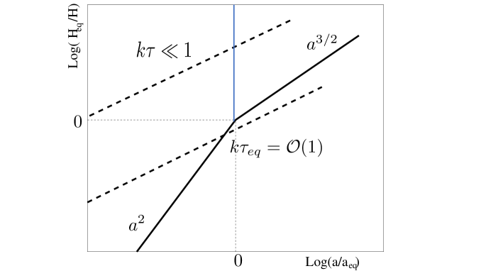
Figure 3: The evolution of the particle horizon is illustrated together with the physical scales determining the initial conditions of the Einstein-Boltzmann hierarchy.

By schematically illustrating the evolution of the Hubble radius across matter-radiation equality, Fig. 3 summarizes the main scales determining the Cauchy data of the Einstein-Boltzmann hierarchy: on the vertical axis the common logarithm of the particle horizon is reported as a function of common logarithm of the scale factor. While the dashed lines in Fig. 3 denote two wavelengths larger than the particle horizon, the scale which is about to cross the Hubble radius corresponds to $k\tau_{\mathrm{eq}}={\mathcal{O}}(1)$. Prior to equality and when the relevant wavelengths of the large-scale fluctuations exceed the particle horizon, the initial conditions of the Einstein-Boltzmann hierarchy are then set: in Fig. 3 this regime corresponds to $\tau<\tau_{\mathrm{eq}}$ (or $a<a_{\mathrm{eq}}$) and $k\tau\ll 1$. The (qualitative) description of large-scale cosmological perturbations [103, 104, 105] stipulates that a given wavelength exits the Hubble radius at some typical conformal time $\tau_{\mathrm{ex}}$ during an inflationary stage of expansion and approximately reenters at $\tau_{\mathrm{re}}$, when the Universe still expands but in a decelerated manner. By a mode being beyond the horizon we only mean that the physical wavenumber is much less than the expansion rate: this does not necessarily have anything to do with causality [127].

3.1 Magnetized scalar modes

The scalar fluctuations of the geometry introduced in Eq. (2.34) are subjected to the Hamiltonian constraint (imposing a relation between the density contrasts of the various species of the plasma) and to the momentum constraint (determining a specific relation among the peculiar velocities of the different species). Because of the simultaneous presence of two constraints the analysis is comparatively more challenging than in the case of the vector modes (where only the momentum constraint survives) and of the tensor inhomogeneities (where there are no constraints). The notion of the magnetized initial conditions for the scalar modes of the Einstein-Boltzmann hierarchy has been firstly discussed and pursued Ref. [109] by using the complementary descriptions provided by the longitudinal and synchronous gauges introduced in Eqs. (2.41) and (2.42). While the conformally Newtonian description is free from spurious gauge modes, the synchronous description is more suitable for the numerical treatment of the problem.

During the past decade the analysis of the magnetized scalar modes converged to the same standard employed when constraining more standard sets of initial data like, for instance, the four non-adiabatic modes [110, 111]. The non-Gaussian effects associated with the scalar modes have been firstly scrutinized in [128]. The first calculations of the temperature and polarization anisotropies induced by the magnetized adiabatic mode can be found in [136] and other explicit calculations have been reported in Refs. [137, 138]. Beside the magnetized adiabatic mode [109] also the entropic solutions have been generalized to accommodate the presence of magnetic random fields. While the latter solutions have been comparatively less studied than their adiabatic counterpart, the non-adiabatic modes in combinations with the magnetic contribution may interfere either constructively or destructively but so far no explicit bounds on these solutions have been discussed besides the ones reported in [112].

3.1.1 Strongly interacting species

In the Vlasov-Landau approach (appropriately extended to curved backgrounds) the evolution equations for the distribution functions for electrons and ions can be written as:

$$\partial_{\tau}f_{\mathrm{e,i}}+\vec{v}\cdot\vec{\nabla}_{\vec{x}}f_{\mathrm{e,i}}\mp e\bigl{[}\vec{E}+\vec{v}\times\vec{B}\bigr{]}\cdot\vec{\nabla}_{\vec{q}}f_{\mathrm{e,i}}=\bigl{[}\partial_{\tau}f_{\mathrm{e,i}}\bigr{]}_{\mathrm{coll}},$$ (3.1)

where $\vec{B}$, $\vec{E}$ and $\vec{v}$ are, respectively, the comoving electromagnetic fields and the peculiar velocity already defined in Eqs. (2.21) and (2.22); in the non-relativistic limit (which is the relevant one in the case of Eq. (3.1) the comoving three-momentum is $\vec{q}=ma\vec{v}$ and $m$ is the mass of the charge carrier (i.e. either electron or ion). The collisional terms at the right hand side of Eq. (3.1) are different for electrons and ions. By perturbing Eq. (3.1) around a solution describing an approximate kinetic equilibrium, the evolution of the various moments of the (perturbed) distribution functions can be derived and they will lead, respectively, to the equations for charge concentration (from the zeroth-order moment), to the equations for the velocities (from the first-order moment) and so on. In the flat space-time case this analysis is well known and can be found, for instance, in [55, 57]. Defining the charge concentrations and the velocities as appropriate moments of the distribution function

$$n_{\mathrm{e}}(\vec{x},\tau)=n_{0}\int d^{3}vf_{\mathrm{e}}(\vec{x},\vec{v},\tau),\qquad n_{\mathrm{i}}(\vec{x},\tau)=n_{0}\int d^{3}vf_{\mathrm{i}}(\vec{x},\vec{v},\tau),$$ (3.2)

$$\vec{v}_{\mathrm{e}}(\vec{x},\tau)=n_{0}\int d^{3}v\,\vec{v}\,f_{\mathrm{e}}(\vec{x},\vec{v},\tau),\qquad\vec{v}_{\mathrm{i}}(\vec{x},\tau)=n_{0}\int d^{3}v\,\vec{v}\,f_{\mathrm{i}}(\vec{x},\vec{v},\tau),$$ (3.3)

the evolution of the zeroth-order moment of Eq. (3.1) implies the evolution equation of the charge concentrations:

$$\partial_{\tau}n_{\mathrm{i}}+\theta_{\mathrm{i}}n_{\mathrm{i}}+\vec{v}_{\mathrm{i}}\cdot\vec{\nabla}n_{\mathrm{i}}=0,\qquad\partial_{\tau}n_{\mathrm{e}}+\theta_{\mathrm{e}}n_{\mathrm{e}}+\vec{v}_{\mathrm{e}}\cdot\vec{\nabla}n_{\mathrm{e}}=0,$$ (3.4)

where $\theta_{\mathrm{i}}=\vec{\nabla}\cdot\vec{v}_{\mathrm{i}}$ and $\theta_{\mathrm{e}}=\vec{\nabla}\cdot\vec{v}_{\mathrm{e}}$ are the three-divergences of the comoving three-velocities.

Even if the equations for the velocities follow in a similar manner from Eqs. (3.1) and (3.2)–(3.3), the same results of the Vlasov-Landau approach can be derived by perturbing (to first order) the covariant momentum conservation:

$$\nabla_{\mu}T^{\mu\nu}_{(\mathrm{i})}=F^{\nu\alpha}j_{\alpha}^{(\mathrm{i})}+(\rho_{\gamma}+p_{\gamma})\,\Gamma_{\gamma\mathrm{i}}[u_{(\gamma)}^{\nu}-u_{(\mathrm{i})}^{\nu}]+\rho_{\mathrm{e}}\Gamma_{\mathrm{ei}}[u_{(\mathrm{e})}^{\nu}-u_{(\mathrm{i})}^{\nu}],$$ (3.5)

$$\nabla_{\mu}T^{\mu\nu}_{(\mathrm{e})}=F^{\nu\alpha}j_{\alpha}^{(\mathrm{e})}+(\rho_{\gamma}+p_{\gamma})\,\Gamma_{\gamma\mathrm{e}}[u_{(\gamma)}^{\nu}-u_{(\mathrm{e})}^{\nu}]+\rho_{\mathrm{e}}\Gamma_{\mathrm{ei}}[u_{(\mathrm{i})}^{\nu}-u_{(\mathrm{e})}^{\nu}],$$ (3.6)

$$\nabla_{\mu}T^{\mu\nu}_{(\gamma)}=\Gamma_{\gamma\mathrm{i}}(\rho_{\gamma}+p_{\gamma})[u_{(\mathrm{i})}^{\nu}-u_{(\gamma)}^{\nu}]+\Gamma_{\gamma\mathrm{e}}(\rho_{\gamma}+p_{\gamma})[u_{(\mathrm{e})}^{\nu}-u_{(\gamma)}^{\nu}],$$ (3.7)

where the expressions of $T^{\mu\nu}_{(\mathrm{i})}$, $T^{\mu\nu}_{(\mathrm{e})}$ and $T^{\mu\nu}_{(\gamma)}$ have been already introduced in Eqs. (2.10) and (2.11). Since the first-order scalar fluctuations of $\nabla_{\mu}T^{\mu\nu}$ for a generic energy-momentum tensor is given by:

$$\delta_{\mathrm{s}}\nabla_{\mu}T^{\mu\nu}=\partial_{\mu}\delta_{\mathrm{s}}T^{\mu\nu}+\delta_{\mathrm{s}}\Gamma^{\mu}_{\mu\alpha}\overline{T}^{\alpha\nu}+\overline{\Gamma}^{\mu}_{\mu\alpha}\delta_{\mathrm{s}}T^{\alpha\nu}+\delta_{\mathrm{s}}\Gamma^{\nu}_{\alpha\beta}\overline{T}^{\alpha\beta}+\overline{\Gamma}^{\nu}_{\alpha\beta}\delta_{\mathrm{s}}T^{\alpha\beta},$$ (3.8)

the evolution equations of the velocities and of the density contrasts can be obtained from the scalar fluctuations of the Christoffel connections expressed in the longitudinal gauge of Eq. (2.41) (see e.g. [105]). The notation $\delta_{\mathrm{s}}$ has been already introduced after Eq. (2.34). In appendix C the main equations of the present section will be studied in the synchronous coordinate system already defined in Eq. (2.42).

If the free tensor index $\nu$ of Eqs. (3.5)–(3.7) is space-like, we obtain the evolution equations of the peculiar velocities for electrons, ions and photons:

$$\vec{v}_{\mathrm{e}}^{\,\prime}+{\mathcal{H}}\,\vec{v}_{\mathrm{e}}=-\frac{e}{m_{\mathrm{e}}\,a}[\vec{E}+\vec{v}_{\mathrm{e}}\times\vec{B}]-\vec{\nabla}\phi+\frac{4}{3}\frac{\rho_{\gamma}}{\rho_{\mathrm{e}}}a\Gamma_{\gamma\,\mathrm{e}}(\vec{v}_{\gamma}-\vec{v}_{\mathrm{e}})+a\Gamma_{\mathrm{e\,i}}(\vec{v}_{\mathrm{i}}-\vec{v}_{\mathrm{e}}),$$ (3.9)

$$\vec{v}_{\mathrm{i}}^{\,\prime}+{\mathcal{H}}\,\vec{v}_{\mathrm{i}}=\frac{e}{m_{\mathrm{i}}\,a}[\vec{E}+\vec{v}_{\mathrm{i}}\times\vec{B}]-\vec{\nabla}\phi+\frac{4}{3}\frac{\rho_{\gamma}}{\rho_{\mathrm{i}}}a\Gamma_{\gamma\,\mathrm{i}}(\vec{v}_{\gamma}-\vec{v}_{\mathrm{i}})+a\Gamma_{\mathrm{e\,i}}\frac{\rho_{\mathrm{e}}}{\rho_{\mathrm{i}}}(\vec{v}_{\mathrm{e}}-\vec{v}_{\mathrm{i}}),$$ (3.10)

$$\vec{v}_{\gamma}^{\,\prime}=-\frac{1}{4}\vec{\nabla}\delta_{\gamma}-\vec{\nabla}\phi+a\Gamma_{\gamma\mathrm{i}}(\vec{v}_{\mathrm{i}}-\vec{v}_{\gamma})+a\Gamma_{\gamma\mathrm{e}}(\vec{v}_{\mathrm{e}}-\vec{v}_{\gamma}),$$ (3.11)

where $\Gamma_{\gamma\mathrm{e}}$, $\Gamma_{\gamma\mathrm{i}}$ and $\Gamma_{\mathrm{e\,i}}$ are, respectively, the electron-photon, the ion-photon and the electron-ion interaction rates [55, 57]. The peculiar velocities of the various species follow the notations already introduced in Eqs.(2.20) and (2.22). In Eq. (3.11) and in what follows the density contrasts and the divergence of the three-velocities will be denoted, respectively, by by $\delta_{X}=\delta_{\mathrm{s}}\rho_{X}/\rho_{X}$ and $\theta_{X}=\vec{\nabla}\cdot\vec{v}_{X}$ where $X$ is one of the different species of the plasma. Obviously the density contrasts and the peculiar velocities change from one gauge to the other and, in particular, from the longitudinal to the synchronous gauges and vice versa (see, in particular, Eqs. (C.1) and (C.2)).

When the free tensor index appearing in Eqs. (3.5), (3.6) and (3.7) is taken to be time-like (i.e. $\nu=0$) the evolution equations of the density contrasts of the strongly interacting species turn out to be:

$$\delta_{\mathrm{e}}^{\prime}=-\theta_{\mathrm{e}}+3\psi^{\prime}-\frac{e}{m_{\mathrm{e}}a}\vec{E}\cdot\vec{v}_{\mathrm{e}},\qquad\vec{\nabla}\cdot\vec{v}_{\mathrm{e}}=\theta_{\mathrm{e}},$$ (3.12)

$$\delta_{\mathrm{i}}^{\prime}=-\theta_{\mathrm{i}}+3\psi^{\prime}+\frac{e}{m_{\mathrm{i}}a}\vec{E}\cdot\vec{v}_{\mathrm{i}},\qquad\vec{\nabla}\cdot\vec{v}_{\mathrm{i}}=\theta_{\mathrm{i}},$$ (3.13)

$$\delta_{\gamma}^{\prime}=4\psi^{\prime}-\frac{4}{3}\theta_{\gamma},\qquad\vec{\nabla}\cdot\vec{v}_{\gamma}=\theta_{\gamma},$$ (3.14)

with the same notations already employed in Eq. (3.4). All in all Eqs. (3.9)–(3.11) and Eqs. (3.12)–(3.14) describe a three-fluid system formed by photons, electrons and ions.

3.1.2 The photon-lepton-baryon fluid

While the Thomson rate increases with the temperature, the Coulomb rate decreases. More precisely, for physical temperatures larger than the eV, we have that $\Gamma_{\mathrm{ei}}/H\propto 10^{11}(\widetilde{T}/\mathrm{eV})^{-1/2}$ while $\Gamma_{\gamma\mathrm{e}}/H\propto 10^{4}(\widetilde{T}/\mathrm{eV})$. The meeting point of the two rates occurs close to the MeV so that, in the regime described by Fig. 3, photons are strongly coupled to the baryon-lepton (or simply baryon) fluid. The governing equations of the baryon fluid follow from the equations for the electrons and the ions. In particular, by summing Eq. (3.9) (multiplied by $m_{\mathrm{e}}$) and Eq. (3.10) (multiplied by $m_{\mathrm{i}}$) the baryon and the photon velocities will obey, respectively, the following pair of equations:

$$\vec{v}_{\mathrm{b}}^{\,\prime}+{\mathcal{H}}\vec{v}_{\mathrm{b}}=\frac{\vec{J}\times\vec{B}}{a^{4}\rho_{\mathrm{b}}(1+m_{\mathrm{e}}/m_{\mathrm{i}})}-\vec{\nabla}\phi+\frac{\epsilon^{\prime}}{R_{\mathrm{b}}}(\vec{v}_{\gamma}-\vec{v}_{\mathrm{b}}),$$ (3.15)

$$\vec{v_{\gamma}}^{\prime}=-\frac{1}{4}\vec{\nabla}\delta_{\gamma}-\vec{\nabla}\phi+\epsilon^{\prime}(\vec{v}_{\mathrm{b}}-\vec{v}_{\gamma}),$$ (3.16)

$R_{\mathrm{b}}$ and $\epsilon^{\prime}$ denote, respectively, the baryon to photon ratio of Eq. (2.50) and the differential optical depth introduced in Eq.(2.58). The two new one-fluid variables of Eqs. (3.15)–(3.16) are the centre of mass velocity of the electron-ion system and the total comoving current:

$$\vec{v}_{\mathrm{b}}=\frac{m_{\mathrm{e}}\vec{v}_{\mathrm{e}}+m_{\mathrm{i}}\vec{v}_{\mathrm{i}}}{m_{\mathrm{e}}+m_{\mathrm{i}}},\qquad\vec{J}=e\,n_{0}(\vec{v}_{\mathrm{i}}-\vec{v}_{\mathrm{e}}),$$ (3.17)

where $\vec{J}$ (already introduced in Eqs. (2.18)–(2.20)) has been explicitly written in the globally neutral case. The evolution equation of the baryonic density contrast $\delta_{\mathrm{b}}$ follows instead from the sum of Eqs. (3.12) and (3.13) :

$$\delta_{\mathrm{b}}^{\prime}=-\theta_{\mathrm{b}}+3\psi^{\prime}+\frac{\vec{J}\cdot\vec{E}}{a^{4}\rho_{\mathrm{b}}},\qquad\delta_{\mathrm{b}}=\frac{m_{\mathrm{e}}}{m_{\mathrm{i}}+m_{\mathrm{e}}}\delta_{\mathrm{e}}+\frac{m_{\mathrm{i}}}{m_{\mathrm{i}}+m_{\mathrm{e}}}\delta_{\mathrm{i}},$$ (3.18)

where, as before, $\theta_{\mathrm{b}}=\vec{\nabla}\cdot\vec{v}_{\mathrm{b}}$ and $\rho_{\mathrm{b}}=\widetilde{n}_{0}(m_{\mathrm{i}}+m_{\mathrm{e}})$ denotes the physical (not comoving) baryonic matter density in the globally neutral case. It is relevant to remark, as already mentioned in section 2 that the system is not Weyl invariant. The most convenient solution to exploit the remaining symmetries of the equations is therefore to use as much as possible comoving currents and comoving electromagnetic fields (as in Eqs. (3.15), (3.16) and (3.18)) together with the physical energy densities and pressures which appear directly in the background evolution equations (2.13) and (2.14).

Since the photon and the baryon velocities are quickly synchronized because of the hierarchy between the photon-electron rate and the Hubble rate, prior to decoupling the system of Eqs. (3.15), (3.16) and (3.18) can be further combined to eliminate the momentum exchange between photons and baryons:

$$\delta_{\gamma}^{\prime}=4\psi^{\prime}-\frac{4}{3}\theta_{\gamma\mathrm{b}},\qquad\delta_{\mathrm{b}}^{\prime}=3\psi^{\prime}-\theta_{\gamma\mathrm{b}}+\frac{\vec{J}\cdot\vec{E}}{a^{4}\rho_{\mathrm{b}}},$$ (3.19)

$$\theta_{\gamma\mathrm{b}}^{\,\prime}+\frac{{\mathcal{H}}R_{\mathrm{b}}}{R_{\mathrm{b}}+1}\theta_{\gamma\mathrm{b}}-\frac{\eta\,\nabla^{2}\theta_{\gamma\mathrm{b}}}{\rho_{\gamma}(1+R_{\mathrm{b}})}=\frac{3\vec{\nabla}\cdot(\vec{J}\times\vec{B})}{4a^{4}\rho_{\gamma}(R_{\mathrm{b}}+1)}-\frac{\nabla^{2}\delta_{\gamma}}{4(1+R_{\mathrm{b}})}-\nabla^{2}\phi,$$ (3.20)

where $\theta_{\gamma\mathrm{b}}=\vec{\nabla}\cdot\vec{v}_{\gamma\mathrm{b}}$ is the three-divergence of the corresponding peculiar velocity. The shear viscosity term $\eta=(4/15)\rho_{\gamma}\lambda_{\gamma\mathrm{e}}$ (see Eq. (3.20)), depends upon the photon mean free path $\lambda_{\gamma\mathrm{e}}$ which is inversely proportional to the differential optical depth $\epsilon^{\prime}$.

While in the limit $\vec{J}\to 0$ Eqs. (3.19) and (3.20) reproduce the conventional system of equations, in the present situation the electric fields and the total currents are essential. The simplest way of addressing this problem is to resort to the magnetohydrodynamical reduction [57, 59, 61], as originally suggested in [109, 136] and subsequently discussed by different authors (see e.g. [137, 138]). The cumbersome expression obtained by taking the difference of Eq. (3.9) (multiplied by $e\,n_{\mathrm{i}}$) and of Eq. (3.10) (multiplied by $e\,n_{\mathrm{e}}$) can be simplified in the limit $(m_{\mathrm{e}}/m_{\mathrm{i}})\ll 1$. Furthermore, since the plasma is globally neutral, the final result of this procedure translates into a differential form of the Ohm law reading [139]:

$$\partial_{\tau}\vec{J}+\biggl{(}{\mathcal{H}}+a\Gamma_{\mathrm{ie}}+\frac{4\rho_{\gamma}\Gamma_{\mathrm{e}\gamma}}{3n_{0}\,m_{\mathrm{e}}}\biggr{)}\vec{J} = \frac{\overline{\omega}_{\mathrm{pe}}^{2}}{4\pi}\biggl{(}\vec{E}+\vec{v}_{\mathrm{b}}\times\vec{B}+\frac{\vec{\nabla}p_{\mathrm{e}}}{e\,n_{0}}-\frac{\vec{J}\times\vec{B}}{en_{0}}\biggr{)}$$ (3.21)

$$+ \frac{4e\rho_{\gamma}\Gamma_{\mathrm{e}\gamma}}{3m_{\mathrm{e}}}(\vec{v}_{\mathrm{b}}-\vec{v}_{\gamma}).$$

The terms $\partial_{\tau}\vec{J}$ and ${\mathcal{H}}\vec{J}$ are comparable in magnitude; moreover they are both smaller than $\Gamma_{\mathrm{ie}}$ and $\Gamma_{\mathrm{e}\gamma}$, i.e. ${\mathcal{H}}\vec{J}\simeq\partial_{\tau}\vec{J}<(4/3)(\rho_{\gamma}/m_{\mathrm{e}})\Gamma_{\mathrm{e}\gamma}<a\Gamma_{\mathrm{ie}}$. Since Eq. (3.21) is dominated by the Coulomb rate $\Gamma_{\mathrm{ie}}$, at the right-hand side the term containing $(\vec{v}_{\mathrm{b}}-\vec{v}_{\gamma})$ is estimated by subtracting Eqs. (3.15) and (3.16); this term is driven exponentially to zero at a rate controlled by $a\Gamma_{\gamma\mathrm{e}}(1+R_{\mathrm{b}}^{-1})$. The Ohm’s law (in its asymptotic form) becomes then:

$$\vec{J}=\sigma\biggl{(}\vec{E}+\vec{v}_{\gamma\mathrm{b}}\times\vec{B}+\frac{\vec{\nabla}p_{\mathrm{e}}}{e\,n_{0}}-\frac{\vec{J}\times\vec{B}}{e\,n_{0}}\biggr{)},$$ (3.22)

where $\sigma$ denotes the comoving conductivity whose explicit form turns out to be:

$$\sigma=\frac{\overline{\omega}_{\mathrm{pe}}^{2}}{4\pi\{a\Gamma_{\mathrm{ie}}+(4/3)[\rho_{\gamma}/(n_{0}m_{\mathrm{e}})]\Gamma_{\mathrm{e}\gamma}\}}\to\frac{9}{8\pi\sqrt{3}}\frac{T}{e^{2}}\sqrt{\frac{T}{m_{\mathrm{e}}a}}[\ln{\Lambda_{\mathrm{C}}(T)}]^{-1},$$ (3.23)

where, as in Eq. (2.3), $\Lambda_{\mathrm{C}}=1.102\times(h_{0}^{2}\Omega_{\mathrm{b}0}/0.02273)^{-1/2}$ is the argument of the Coulomb logarithm; the second limit in Eq. (3.23) follows when the Coulomb rate dominates.

The hierarchy of scales leading to the simplification of Eq. (3.22) also implies that the displacement current of Eq. (2.20) is negligible in comparison with the Ohmic current. Since $4\pi\vec{J}\gg\partial_{\tau}\vec{E}$ the general form of Eqs. (2.19) and (2.20) gets much simpler since the electric fields, the magnetic fields and the Ohmic current are all solenoidal:

$$\vec{\nabla}\cdot\vec{E}=0,\qquad\vec{\nabla}\cdot\vec{B}=0,\qquad\vec{\nabla}\cdot\vec{J}=0.$$ (3.24)

The term $\vec{J}\cdot\vec{E}$ appearing in Eq. (3.19) can be approximated, in the baryon rest frame, as:

$$\frac{\vec{J}\cdot\vec{E}}{a^{4}\rho_{\mathrm{b}}}=\frac{(\vec{\nabla}\times\vec{B})^{2}}{4\pi\sigma a^{4}\rho_{\mathrm{b}}},\qquad\vec{E}\simeq\frac{\vec{\nabla}\times\vec{B}}{4\pi\sigma}.$$ (3.25)

Moreover, since Eq. (3.23) implies that $\sigma/\overline{\omega}_{\mathrm{pe}}\gg 1$ (and also that $\sigma/T\gg 1$), the large-scale electric fields are highly suppressed by powers of $\sigma^{-1}$ in the baryon rest frame [139] and can be estimated, from Eq. (3.22). The corresponding evolution equation for the magnetic field becomes then:

$$\partial_{\tau}\vec{B}=\vec{\nabla}\times(\vec{v}_{\gamma\mathrm{b}}\times\vec{B})+\frac{1}{4\pi\sigma}\nabla^{2}\vec{B}+\vec{\nabla}\times\biggl{[}\frac{\vec{\nabla}p_{e}}{en_{0}}\biggr{]}-\vec{\nabla}\times\biggl{[}\frac{(\vec{\nabla}\times\vec{B})\times\vec{B}}{4\pi en_{0}}\biggr{]},$$ (3.26)

where, to avoid ambiguities, the primes (denoting a derivation with respect to $\tau$) have been replaced by $\partial_{\tau}$. If the thermoelectric and Hall terms are neglected in Eq. (3.26) we obtain the standard form of the magnetic diffusivity equation where the bulk velocity of the plasma coincides with the baryon-photon velocity. By making explicit Eq. (3.22) in terms of the electric field and by taking the first conformal time derivative of the obtained expression we have an equation formally similar to Eq. (3.26):

$$\partial_{\tau}\vec{E}=-\partial_{\tau}(\vec{v}_{\gamma\mathrm{b}}\times\vec{B})+\frac{\partial_{\tau}\vec{J}}{\sigma}-\partial_{\tau}\biggl{[}\frac{\vec{\nabla}p_{e}}{en_{0}}\biggr{]}-\partial_{\tau}\biggl{[}\frac{(\vec{\nabla}\times\vec{B})\times\vec{B}}{4\pi en_{0}}\biggr{]},$$ (3.27)

where, to lowest order, $\partial_{\tau}\vec{J}=-\vec{\nabla}\times(\vec{\nabla}\times\vec{E})/(4\pi)$. Neglecting now the thermoelectric and the Hall terms in Eqs. (3.26) and (3.27) we can obtain the following simplified description:

$$\partial_{\tau}\vec{B}=\vec{\nabla}\times(\vec{v}_{\gamma\mathrm{b}}\times\vec{B})+\frac{1}{4\pi\sigma}\nabla^{2}\vec{B},\qquad\partial_{\tau}\vec{E}=-\partial_{\tau}(\vec{v}_{\mathrm{b}}\times\vec{B})+\frac{1}{4\pi\sigma}\nabla^{2}\vec{E}.$$ (3.28)

Before recombination denoting with $\tau_{\mathrm{c}}$ the inverse of the differential optical depth (i.e. $\tau_{\mathrm{c}}=1/\epsilon^{\prime}$), an explicit evolution equations for the velocity differences between baryons and photons can be derived by including the effects of the magnetic random fields. In the tight-coupling approximation, we have that the baryon and photon velocities coincide, at least approximately, i.e. $\theta_{\gamma\mathrm{b}}\simeq\theta_{\gamma}\simeq\theta_{\mathrm{b}}$. When the tight-coupling approximation breaks down it is possible to derive an evolution equation for $(\theta_{\mathrm{b}}-\theta_{\gamma})$ valid for $|\tau_{\mathrm{c}}/\tau|\ll 1$ and $k\tau_{c}\ll 1$. The idea of treating the problem in this way is due to Peebles and Yu [49] and has been subsequently rediscovered, for numerical purposes, in Ref. [67, 129, 130, 131].

3.1.3 Weakly interacting constituents

While the evolution of the CDM fluctuations only consists of the following two equations:

$$\delta_{\mathrm{c}}^{\prime}=3\psi^{\prime}-\theta_{\mathrm{c}},\qquad\theta_{\mathrm{c}}^{\,\prime}+{\mathcal{H}}\theta_{\mathrm{c}}=-\nabla^{2}\phi,$$ (3.29)

the neutrinos obey the collisionless Boltzmann equation whose lowest multipoles obey the following triplet of equations in Fourier space

$$\delta_{\nu}^{\prime}=-\frac{4}{3}\theta_{\nu}+4\psi^{\prime},$$ (3.30)

$$\theta_{\nu}^{\prime}=-k^{2}\sigma_{\nu}+\frac{k^{2}}{4}\delta_{\nu}+k^{2}\phi,$$ (3.31)

$$\sigma_{\nu}^{\prime}=\frac{4}{15}\theta_{\nu}-\frac{3}{10}k{\mathcal{F}}_{\nu 3},$$ (3.32)

where ${\mathcal{F}}_{\nu 3}$ is the octupole of the full neutrino phase space distribution. The collisionless Boltzmann equation supplemented by the contribution of the geometry is given by

$$\partial_{\tau}{\mathcal{F}}_{\nu}+ik\mu{\mathcal{F}}_{\nu}=4(\psi^{\prime}-ik\mu\phi).$$ (3.33)

The notations used in Eqs. (3.30)–(3.32) and (3.33) coincide with the ones of Refs. [109, 136]; these notations are essentially the ones of Ref. [67] (the signature of the metric (1.5) is however different and the longitudinal potentials of Eq. (2.41) are defined in a slightly different manner). If we expand the angular dependence of the reduced phase-space distribution in series of Legendre polynomials

$${\mathcal{F}}_{\nu}(\vec{k},\hat{n},\tau)=\sum_{\ell}(-i)^{\ell}(2\ell+1){\mathcal{F}}_{\nu\ell}(\vec{k},\tau)P_{\ell}(\mu),$$ (3.34)

Eqs. (3.30), (3.31) and (3.32) correspond, up to trivial numerical factors, to the evolution of the monopole, dipole and quadrupole of ${\mathcal{F}}_{\nu}$. For higher multipoles (i.e. $\ell\geq 3$)

$${\mathcal{F}}_{\nu\ell}^{\prime}=\frac{k}{2\ell+1}[\ell{\mathcal{F}}_{\nu,(\ell-1)}-(\ell+1){\mathcal{F}}_{\nu(\ell+1)}].$$ (3.35)

Note that in Eqs. (3.31) and (3.32), $\sigma_{\nu}$ is related to the neutrino anisotropic stress as $\partial_{i}\partial_{j}\Pi_{\mathrm{f}}^{ij}=(p_{\nu}+\rho_{\nu})\nabla^{2}\sigma_{\nu}$ where $\Pi_{\mathrm{f}}^{ij}$ is the anisotropic stress of the fluid. These two quantities coincide within the $\Lambda$CDM paradigm where the only source of anisotropic stress of the fluid is represented by the massless neutrinos. While in the concordance scenario the dark energy component does not fluctuate, it is often interesting to investigate the stability of the magnetized initial conditions in the presence of a fluctuating dark energy component which, among other things, may affect the integrated Sachs-Wolfe effect. Two supplementary evolution equations must be considered in this case and they correspond to the evolution of the dark energy density contrast and of the peculiar velocity.

3.1.4 The fluctuations of the geometry

The weakly interacting species are affected by the magnetic random fields through the evolution of the fluctuations of the geometry obeying the inhomogeneous Einstein equations. By perturbing both sides of Eq. (2.8) with respect to the scalar fluctuations of the geometry (1.5) we have

$$\delta_{\mathrm{s}}R_{\mu}^{\nu}-\frac{1}{2}\delta_{\mu}^{\nu}\,\delta_{\mathrm{s}}R=\ell_{P}^{2}\,\delta_{\mathrm{s}}T_{\mu}^{\nu},$$ (3.36)

where $\delta_{\mathrm{s}}$ denotes the scalar fluctuation of the coresponding tensor, exactly as in Eq. (2.34). The $(00)$ and $(0i)$ components of Eq. (3.36) relate the scalar fluctuations of the geometry to their first derivatives. In particular, denoting by $\delta_{\mathrm{s}}\rho_{\mathrm{t}}$ the total fluctuation of the energy density in the gauge (2.41),

$$\delta_{\mathrm{s}}\rho_{\mathrm{t}}=\delta_{\mathrm{s}}\rho_{\mathrm{c}}+\delta_{\mathrm{s}}\rho_{\nu}+\delta_{\mathrm{s}}\rho_{\gamma}+\delta_{\mathrm{s}}\rho_{\mathrm{b}},$$ (3.37)

the Hamiltonian constraint

$$\nabla^{2}\psi-3{\mathcal{H}}({\mathcal{H}}\phi+\psi^{\prime})=\frac{\ell_{P}^{2}a^{2}}{2}\biggl{[}\delta_{\mathrm{s}}\rho_{\mathrm{t}}+\delta_{\mathrm{s}}\rho_{\mathrm{B}}+\delta_{\mathrm{s}}\rho_{{\mathrm{E}}}\biggr{]},$$ (3.38)

follows from the $(00)$ component of Eq. (3.36). The fluctuations of the electromagnetic energy density and of the corresponding pressure are preceded by $\delta_{\mathrm{s}}$ since, unlike the corresponding anisotropic stresses, they only affect the evolution of the scalar modes:

$$\delta_{\mathrm{s}}\rho_{\mathrm{B}}=\frac{B^{2}}{8\pi a^{4}},\qquad\delta_{\mathrm{s}}\rho_{\mathrm{E}}=\frac{E^{2}}{8\pi a^{4}},\qquad\delta_{\mathrm{s}}p_{\mathrm{B}}=\frac{\delta_{\mathrm{s}}\rho_{\mathrm{B}}}{3},\qquad\delta_{\mathrm{s}}p_{\mathrm{E}}=\frac{\delta_{\mathrm{s}}\rho_{\mathrm{E}}}{3}.$$ (3.39)

The magnetic and electric energy densities are customarily referred to the energy density of the photon background [109, 136] by introducing the following dimensionless variables:

$$\Omega_{\mathrm{E}}(\vec{x},\tau)=\frac{\delta_{s}\rho_{\mathrm{E}}(\vec{x},\tau)}{\rho_{\gamma}(\tau)},\qquad\Omega_{\mathrm{B}}(\vec{x},\tau)=\frac{\delta_{s}\rho_{\mathrm{B}}(\vec{x},\tau)}{\rho_{\gamma}(\tau)}.$$ (3.40)

Since the total three-velocity field is not solenoidal in the case of the scalar modes, from the $(0i)$ component of Eq. (3.36) we can write the three-divergence of the momentum constraint

$$\nabla^{2}({\mathcal{H}}\phi+\psi^{\prime})+\frac{\ell_{P}^{2}a^{2}}{2}\biggl{[}(p_{\mathrm{t}}+\rho_{\mathrm{t}})\theta_{\mathrm{t}}+\frac{\vec{\nabla}\cdot(\vec{E}\times\vec{B})}{4\pi a^{4}}\biggr{]}=0,$$ (3.41)

where $\theta_{\mathrm{t}}$ denotes the total velocity field:

$$(p_{\mathrm{t}}+p_{\mathrm{t}})\theta_{\mathrm{t}} = \sum_{a}(p_{\mathrm{a}}+\rho_{\mathrm{a}})\theta_{\mathrm{a}}\equiv\frac{4}{3}\rho_{\nu}\theta_{\nu}+\frac{4}{3}\rho_{\gamma}\theta_{\gamma}+\rho_{\mathrm{c}}\theta_{\mathrm{c}}+\rho_{\mathrm{b}}\theta_{\mathrm{b}}$$ (3.42)

$$= \rho_{\mathrm{c}}\theta_{\mathrm{c}}+\frac{4}{3}\rho_{\nu}\theta_{\nu}+\frac{4}{3}\rho_{\gamma}\theta_{\gamma\mathrm{b}}(1+R_{\mathrm{b}}).$$

The expression appearing in the second line of Eq. (3.42) holds in the tight coupling approximation while the two preceding expressions are general. When the free indices are both space-like, the trace-full part of Eq. (3.36) is dynamical and it is given by:

$$\psi^{\prime\prime}+{\mathcal{H}}(\phi^{\prime}+2\psi^{\prime})+({\mathcal{H}}^{2}+2{\mathcal{H}}^{\prime})\phi+\frac{1}{3}\nabla^{2}(\phi-\psi)=\frac{\ell_{P}^{2}a^{2}}{2}\biggl{[}\delta_{\mathrm{s}}p_{\mathrm{t}}+\delta_{\mathrm{s}}p_{\mathrm{B}}+\delta_{\mathrm{s}}p_{\mathrm{E}}\biggr{]},$$ (3.43)

where $\delta_{\mathrm{s}}p_{\mathrm{t}}$ denotes the fluctuation of the total pressure which can always be expressed as the sum of an adiabatic contribution (containing the total sound speed $c_{\mathrm{st}}$) supplemented by a non-adiabatic (or entropic) fluctuation:

$$\delta_{\mathrm{s}}p_{\mathrm{t}}=c_{\mathrm{st}}^{2}\delta\rho_{\mathrm{t}}+\delta p_{\mathrm{nad}},\qquad c_{\mathrm{st}}^{2}=\frac{p_{\mathrm{t}}^{\prime}}{\rho_{\mathrm{t}}^{\prime}}.$$ (3.44)

Equation (3.44) stipulates that the fluctuations of the total pressure can either arise as fluctuations of the total energy density or as fluctuations of the chemical content of the plasma: $\delta p_{\mathrm{nad}}$ denotes the non-adiabatic fluctuation of the total pressure [110, 111, 112] and it can only appear if the plasma contains, at least, two different species. The last equation to be discussed is the traceless part of the $(ij)$ component of Eq. (3.36):

$$\partial^{i}\partial^{j}(\phi-\psi)-\frac{\delta^{ij}}{3}\nabla^{2}(\phi-\psi)=\ell_{P}^{2}a^{2}\Pi^{ij}_{\mathrm{tot}},\qquad\Pi^{ij}_{\mathrm{tot}}=\Pi^{ij}_{\mathrm{f}}+\Pi_{\mathrm{E}}^{ij}+\Pi_{\mathrm{B}}^{ij},$$ (3.45)

where $\Pi^{ij}_{\mathrm{tot}}$ denotes the total anisotropic stress of the system written as the sum of a fluid component and of the electromagnetic components:

$$\Pi_{\mathrm{E}\,i}^{j}=\frac{1}{4\pi a^{4}}\biggl{[}E_{i}E^{j}-\frac{\delta_{i}^{j}}{3}E^{2}\biggr{]},\qquad\Pi_{\mathrm{B}\,i}^{j}=\frac{1}{4\pi a^{4}}\biggl{[}B_{i}B^{j}-\frac{\delta_{i}^{j}}{3}B^{2}\biggr{]}.$$ (3.46)

A transparent relation between the longitudinal fluctuations and the sources of anisotropic stress can be obtained by applying two spatial gradients to both sides of Eq. (3.45):

$$\nabla^{2}(\phi-\psi)=\frac{3}{2}\ell_{P}^{2}a^{2}\Pi_{\mathrm{tot}},\qquad\partial_{i}\partial_{j}\Pi^{ij}_{\mathrm{tot}}=\nabla^{2}\Pi_{\mathrm{tot}},\qquad\Pi_{\mathrm{tot}}=\Pi_{\mathrm{E}}+\Pi_{\mathrm{B}}+\Pi_{\mathrm{f}}.$$ (3.47)

It is practical to express the electric and magnetic anisotropic stresses in dimensionless terms [109, 136]. Recalling that in the concordance paradigm the dominant source of anisotropic stress is provided by massless neutrinos the anisotropic stresses of Eq. (3.47) can also be expressed as:

$$\partial_{i}\partial_{j}\Pi^{ij}_{\mathrm{f}}=\nabla^{2}\Pi_{\mathrm{f}},\qquad\Pi_{\mathrm{f}}\equiv\Pi_{\nu}=(\rho_{\nu}+p_{\nu})\sigma_{\nu},$$ (3.48)

$$\partial_{i}\partial_{j}\Pi^{ij}_{\mathrm{E}}=\nabla^{2}\Pi_{\mathrm{E}}=(p_{\gamma}+\rho_{\gamma})\nabla^{2}\sigma_{\mathrm{E}},\qquad\partial_{i}\partial_{j}\Pi^{ij}_{\mathrm{B}}=\nabla^{2}\Pi_{\mathrm{B}}=(p_{\gamma}+\rho_{\gamma})\nabla^{2}\sigma_{\mathrm{B}}.$$ (3.49)

Since $\sigma_{\mathrm{E}}$ and $\sigma_{\mathrm{B}}$ are both dimensionless they are the analog of the dimensionless ratios defined in Eq. (3.40) for the electric and magnetic energy densities. The two sets of variables are related by the vector identities discussed in Eqs. (A.26) and (A.27). The relation $\Pi_{\mathrm{B}}=(p_{\gamma}+\rho_{\gamma})\sigma_{\mathrm{B}}$ is also practical since $\sigma_{\mathrm{B}}$ is the magnetic analog of $\sigma_{\nu}$ introduced in the neutrino case [109, 136] (see also [67] for analog notations in the case of neutrinos).

According to the vector identities discussed in appendix A (see, in particular, Eqs. (A.27) and (A.28)) the magnetohydrodynamical Lorentz force appearing in Eqs. (3.20) can be solely expressed in terms of $\sigma_{\mathrm{B}}$ and $\Omega_{\mathrm{B}}$. Indeed, from Eq. (3.20) we have that

$$\frac{3\vec{\nabla}\cdot(\vec{J}\times\vec{B})}{4a^{4}\rho_{\gamma}(R_{\mathrm{b}}+1)}=\frac{1}{4(R_{\mathrm{b}}+1)}\biggl{[}4\nabla^{2}\sigma_{\mathrm{B}}-\nabla^{2}\Omega_{\mathrm{B}}\biggr{]},\qquad\vec{J}=\frac{\vec{\nabla}\times\vec{B}}{4\pi},$$ (3.50)

where the right hand side follows from the left hand side thanks to Eq. (A.27). This observation reduces the number of correlators by a factor of $2$ [109, 136]. Equation (3.50) is however not universal but only holds in the absence of Ohmic electric fields which can be however included with their relative power spectra. It is finally relevant to mention that there exist magnetic field configurations which are force-free. A typical example are the eigenvecors of the curl, i.e. $\vec{\nabla}\times\vec{B}=\alpha\vec{B}$ originally studied, in the case of constant $\alpha$ within the so-called Chandrasekhar-Kendall representation [141]. More realistic configurations where the gyrotropy does decrease at large distance scales can be found [142]. These situations are even simpler to analyze since, as discussed in [109], the vanishing of the total current implies, according to Eqs. (3.50) and (A.27) that $\Omega_{\mathrm{B}}=4\sigma_{\mathrm{B}}$.

3.1.5 Gauge-invariant quasi-normal modes

In the absence of magnetic and electric fields the Cauchy data of the temperature and polarization anisotropies can be determined with standard methods [67, 129, 130, 131]) by expanding the lowest multipoles of the Einstein-Boltzmann hierarchy in powers of $|k\tau|<1$. While the conventional semianalytic approaches [132, 133, 134, 135] can be generalized to include the presence of magnetic random fields, a more transparent strategy is to solve directly the (gauge-invariant) evolution of the quasi-normal modes of the system and then deduce the metric fluctuations in the wanted coordinate system.

To derive the evolution equations of the quasi-normal modes we first take the difference between Eq. (3.43) and the Hamiltonian constraint of Eq. (3.38) (multiplied by $c_{\mathrm{st}}^{2}$). After some algebra the following first-order equation can be readily obtained:

$${\mathcal{R}}^{\prime}=\Sigma_{{\mathcal{R}}}-\frac{2a^{2}\nabla^{2}\psi}{\ell_{P}^{2}{\mathcal{H}}z_{t}^{2}},\qquad z_{t}=\frac{a^{2}\sqrt{\rho_{\mathrm{t}}+p_{\mathrm{t}}}}{{\mathcal{H}}\,c_{\mathrm{st}}},$$ (3.51)

where ${\mathcal{R}}$ is the curvature perturbation on comoving orthogonal hypersurfaces defined in Eq. (2.46); $\Sigma_{{\mathcal{R}}}$ contains the contribution of the electromagnetic fields, of the non-adiabatic pressure fluctuations and of the total anisotropic stress:

$$\Sigma_{{\mathcal{R}}}=-\frac{{\mathcal{H}}}{p_{t}+\rho_{t}}\delta p_{\mathrm{nad}}+\frac{{\mathcal{H}}}{p_{t}+\rho_{t}}\biggl{[}\biggl{(}c_{\mathrm{st}}^{2}-\frac{1}{3}\biggr{)}(\delta_{\mathrm{s}}\rho_{E}+\delta_{\mathrm{s}}\rho_{B})+\Pi_{\mathrm{tot}}\biggr{]},$$ (3.52)

where, as in Eqs. (3.45) and (3.47), $\Pi_{\mathrm{tot}}$ contains both the electromagnetic and the fluid contributions. By eliminating the longitudinal fluctuations of the metric (i.e. $\phi$ and $\psi$) through the Eq. (2.46), the conformal time derivative of Eq. (3.51) leads to a decoupled equation for ${\mathcal{R}}$:

$${\mathcal{R}}^{\prime\prime}+2\frac{z_{t}^{\prime}}{z_{t}}{\mathcal{R}}^{\prime}-c_{\mathrm{st}}^{2}\nabla^{2}{\mathcal{R}}=\Sigma_{{\mathcal{R}}}^{\prime}+2\frac{z_{t}^{\prime}}{z_{t}}\Sigma_{{\mathcal{R}}}+\frac{3a^{4}}{z_{t}^{2}}\Pi_{\mathrm{tot}}.$$ (3.53)

Eq. (3.53) follows by using the background equations of Eqs. (2.13)–(2.14) together with Eqs. (2.46) and (3.47). The result of Eq. (3.53) has been originally derived in the appendix of Ref. [70] and subsequently applied to various problems [144] involving the inflationary initial conditions of the magnetized curvature perturbations. When $\delta p_{\mathrm{nad}}\to 0$, $\Pi_{\mathrm{tot}}\to 0$ and in the absence of electromagnetic contributions, Eq. (3.53) coincides with the evolution equation of the normal mode of a relativistic irrotational fluid derived by Lukash [73, 74, 75].

Equation (3.53) must be supplemented by the evolution equation for the anisotropic stress. In the concordance scenario the only source of anisotropic stress comes from the neutrino sector; we can then take a conformal time derivative of both sides of Eq. (3.32) and obtain:

$$\sigma_{\nu}^{\prime\prime}=\frac{k^{2}}{15}\delta_{\nu}+\frac{4}{15}k^{2}\phi-\frac{11}{21}k^{2}\sigma_{\nu},$$ (3.54)

where the neutrino hierarchy has been truncated, for illustration, to the octupole (notice, however, that ${\mathcal{F}}_{\nu\,3}^{\prime}\neq 0$). By taking a further conformal time derivative of Eq. (3.54), $\delta_{\nu}^{\prime}$ can be eliminated by means of Eq. (3.30); the term $\phi^{\prime}$ shall be traded for the explicit definition of the total anisotropic stress (3.49). Finally the remaining parts of the equation (proportional to $\psi^{\prime}$) will be easily eliminated by using the second relation of Eq. (2.46) (holding in the longitudinal gauge) together with Eq. (3.51). The final result for the evolution equation of $\sigma_{\nu}$ will then be [144]

$$\sigma_{\nu}^{\prime\prime\prime}+\frac{8}{5}{\mathcal{H}}^{2}R_{\nu}\Omega_{R}\sigma_{\nu}^{\prime}-\frac{6}{7}\nabla^{2}\sigma_{\nu}^{\prime}-\frac{8{\mathcal{H}}}{5\overline{M}_{\mathrm{P}}^{2}}\Pi_{\mathrm{tot}}=\frac{4z_{t}^{2}}{15\overline{M}_{\mathrm{P}}^{2}}\biggl{[}\biggl{(}\frac{{\mathcal{H}}}{a^{2}}\biggr{)}^{\prime}({\mathcal{R}}^{\prime}-\Sigma_{{\mathcal{R}}})+c_{\mathrm{st}}^{2}\biggl{(}\frac{{\mathcal{H}}}{a^{2}}\biggr{)}\nabla^{2}{\mathcal{R}}\biggr{]},$$ (3.55)

where, by definition, $\Pi_{\mathrm{tot}}=[(p_{\nu}+\rho_{\nu})\sigma_{\nu}+(p_{\gamma}+\rho_{\gamma})\sigma_{\mathrm{B}}]$. Note that Eq. (3.55) has been derived under the hypothesis that $R_{\nu}\neq 0$ since we effectively divided both sides of the equation by $R_{\nu}$.

The form of the evolution equations of the quasi-normal modes depend on the field content of the background. While Eq. (3.53) has been obtained in the case of a perfect and irrotational fluid, if the field content changes the quasi-normal modes may obey a slightly different equation. For instance when the gauge kinetic term is coupled, in the action, to a single scalar field as $\lambda(\varphi)F_{\alpha\beta}F^{\alpha\beta}$ the evolution of the magnetized curvature perturbations can be explicitly written in terms of the auxiliary variable $\overline{\Delta}_{{\mathcal{R}}}$:

$$\overline{\Delta}_{{\mathcal{R}}}=\Delta_{{\mathcal{R}}}-\frac{{\mathcal{H}}a^{2}}{\varphi^{\prime\,2}}P,\qquad P=\frac{\vec{\nabla}\cdot(\vec{E}\times\vec{B})}{4\pi a^{4}},$$ (3.56)

where $\Delta_{{\mathcal{R}}}$ is the Laplacian of the curvature perturbations on comoving orthogonal hypersurfaces (i.e. $\Delta_{{\mathcal{R}}}=\nabla^{2}{\mathcal{R}}$) and $P$ is the three-divergence of the Poynting vector. The equation obeyed by $\overline{\Delta}_{{\mathcal{R}}}$ is given by:

$$\overline{\Delta}_{{\mathcal{R}}}^{\prime\prime}+2\frac{z^{\prime}_{\varphi}}{z_{\varphi}}\overline{\Delta}_{{\mathcal{R}}}^{\prime}-\nabla^{2}\overline{\Delta}_{{\mathcal{R}}}={\mathcal{S}},\qquad z_{\varphi}=\frac{a\varphi^{\prime}}{{\mathcal{H}}}.$$ (3.57)

The source term ${\mathcal{S}}$ of Eq. (3.57) is a functional of $P$ and of the fluctuations of the electromagnetic energy density:

$${\mathcal{S}}=\frac{a^{2}}{2\overline{M}_{P}^{2}}\biggl{[}P^{\prime}-\biggl{(}2\frac{{\mathcal{H}}^{\prime}}{{\mathcal{H}}}+2\frac{a^{2}}{\varphi^{\prime}}V_{,\,\varphi}\biggr{)}P+\nabla^{2}(\delta_{\mathrm{s}}\rho_{B}+\delta_{\mathrm{s}}\rho_{E})\biggr{]}+\frac{2a^{2}{\mathcal{H}}{\mathcal{F}}}{\varphi^{\prime\,2}}\nabla^{2}(\delta_{\mathrm{s}}\rho_{B}-\delta_{\mathrm{s}}\rho_{E}),$$ (3.58)

where $V_{,\,\varphi}\equiv\partial V/\partial\varphi$ and $V(\varphi)$ is the scalar potential. When two scalar fields are present, Eq. (3.57) will be replaced by the evolution of two coupled equations [70] which can be more easily deduced in the uniform curvature gauge [68, 69]. Equation (3.58) can be used in a variety of situations and, for instance, during inflation. When the electromagnetic contribution vanishes, Eq. (3.57) reduces to the results of [76, 77] quoted in Eq. (2.45). The continuity of the magnetized perturbations across the inflationary transition has been analyzed in terms of these variables and the related temperature and polarization anisotropies have been computed in [70, 144].

3.1.6 Complementary gauge-invariant descriptions

Since it is well known that the equations obeyed by the two Bardeen potentials [65] coincide with the equations written in the longitudinal gauge where $\Psi\equiv\psi$ and $\Phi\equiv\phi$, every equation written in the longitudinal gauge can be swiftly translated in gauge-invariant terms by using the explicit form of the Bardeen potentials. So, for instance the Hamiltonian constraint of Eq. (3.38) and the definition of ${\mathcal{R}}$ of Eq. (2.46) can be directly expressed in terms of $\Phi$ and $\Psi$ as:

$$\nabla^{2}\Psi-3{\mathcal{H}}({\mathcal{H}}\Phi+\Psi^{\prime})=\frac{\ell_{P}^{2}a^{2}}{2}\biggl{(}\delta^{\mathrm{(gi)}}_{\mathrm{s}}\rho_{\mathrm{t}}+\delta_{\mathrm{s}}\rho_{\mathrm{B}}+\delta_{\mathrm{s}}\rho_{\mathrm{E}}\biggr{)},\qquad{\mathcal{R}}=-\Psi-\frac{{\mathcal{H}}({\mathcal{H}}\Phi+\Psi^{\prime})}{{\mathcal{H}}^{2}-{\mathcal{H}}},$$ (3.59)

where $\delta^{\mathrm{(gi)}}_{\mathrm{s}}\rho_{\mathrm{t}}=\delta_{\mathrm{s}}\rho_{\mathrm{t}}+\rho_{\mathrm{t}}^{\prime}(F-G^{\prime})$ denotes the gauge-invariant fluctuation of the total energy density. The remaining equations of the longitudinal description can all be written in terms of the Bardeen potentials but this extension does not change the properties of the governing equations: if $\phi$ and $\psi$ diverge, the same will be true for $\Phi$ and $\Psi$.

A complementary gauge-invariant description of the magnetized curvature perturbations can be obtained in terms of the density contrast on uniform curvature hypersurfaces:

$$\zeta=-\psi-{\mathcal{H}}\frac{\delta_{\mathrm{s}}\rho_{\mathrm{t}}+\delta_{\mathrm{s}}\rho_{\mathrm{B}}+\delta_{\mathrm{s}}\rho_{\mathrm{E}}}{\rho_{\mathrm{\mathrm{t}}}^{\prime}}\equiv-\Psi-{\mathcal{H}}\frac{\delta_{\mathrm{s}}^{(\mathrm{gi})}\rho_{\mathrm{t}}+\delta_{\mathrm{s}}\rho_{\mathrm{B}}+\delta_{\mathrm{s}}\rho_{\mathrm{E}}}{\rho_{\mathrm{\mathrm{t}}}^{\prime}},$$ (3.60)

where the second equality in Eq. (3.60) follows from the correspondence between Bardeen potentials and longitudinal fluctuations. Alternatively $\zeta$ describes the curvature fluctuations in the hypersurfaces where the total energy density is uniform. In the conventional case many authors do not make any difference between $\zeta$ and ${\mathcal{R}}$. Indeed from the definition of ${\mathcal{R}}$ and $\zeta$ (i.e. Eqs. (2.46) and (3.60)) the Hamiltonian constraint of Eq. (3.38) implies:

$$\zeta-{\mathcal{R}}=\frac{2\nabla^{2}\Psi}{3\ell_{P}^{2}a^{2}(p_{t}+\rho_{t})}=\frac{\Sigma_{\mathcal{R}}-{\mathcal{R}}^{\prime}}{3{\mathcal{H}}c_{\mathrm{st}}^{2}},$$ (3.61)

where the first equation follows from the Hamiltonian constraint while the second relation is obtained by using Eq. (3.51). Thanks to Eq. (3.61) the second-order equation obeyed by $\zeta$ is far more involved than Eq. (2.46) even if the two equations coincide in the $k\tau\ll 1$ limit. The best strategy is probably to compute ${\mathcal{R}}$ from Eq. (3.53) and then calculate ${\mathcal{R}}^{\prime}$; with these two ingredients $\zeta$ can be immediately derived from Eq. (3.61). The first-order equation obeyed by $\zeta$ has been discussed at length in Ref. [136] (see in particular second paper) and it is given by

$$\zeta^{\prime}=\Sigma_{\mathcal{R}}-\frac{{\mathcal{H}}}{p_{\mathrm{t}}+\rho_{\mathrm{t}}}-\frac{\theta_{\mathrm{t}}}{3},$$ (3.62)

where $\theta_{\mathrm{t}}$ denotes the three-divergence of the total velocity field (see Eqs. (3.41) and (3.42)) and the other quantities have been already defined.

3.2 Adiabatic and non-adiabatic initial conditions

In the concordance paradigm, when the dark energy does not fluctuate, there are, overall five different sets of Cauchy data: one adiabatic [67] and four non-adiabatic [110, 111, 112] initial conditions. It can be actually shown on a general ground that the field equations for cosmological perturbations in the Newtonian gauge always have an adiabatic solution, for which ${\mathcal{R}}$ is nonzero and constant in the limit of large wavelength [127]. The four non-adiabatic modes are the CDM radiation mode, the baryon-entropy mode, the neutrino entropy mode and the neutrino isocurvature velocity mode. The solutions of the Einstein-Boltzmann hierarchy must be regular. If they are divergent they may be unphysical unless they can be smoothly described in at least one gauge. The explicit solutions for the adiabatic and non-adiabatic modes can be obtained from Eqs. (3.53) and (3.55) by setting to zero the electromagnetic contributions.

If electromagnetic contribution vanishes in Eq. (3.52) the only source of Eq. (3.53) comes from the entropic fluctuations of plasma and the general form of $\delta p_{\mathrm{nad}}$ is [112]:

$$\delta p_{\mathrm{nad}}(\vec{x},\tau) = \frac{1}{6{\mathcal{H}}\rho_{\mathrm{t}}^{\prime}}\sum_{\mathrm{m\,n}}\rho_{\mathrm{m}}^{\prime}\rho_{\mathrm{n}}^{\prime}(c_{\mathrm{sm}}^{2}-c_{\mathrm{sn}}^{2}){\mathcal{S}}_{\mathrm{mn}},\qquad{\mathcal{S}}_{\mathrm{mn}}=-(\zeta_{\mathrm{m}}-\zeta_{\mathrm{n}}),$$

$$\zeta_{\mathrm{m}} = -\Psi+\frac{\delta^{(\mathrm{gi})}_{\mathrm{m}}}{3(w_{\mathrm{m}}+1)},\qquad\zeta_{\mathrm{n}}=-\Psi+\frac{\delta^{(\mathrm{gi})}_{\mathrm{n}}}{3(w_{\mathrm{n}}+1)},$$ (3.63)

where the indices m and n are not tensor indices but denote two generic species of the plasma; $c_{\mathrm{sm}}^{2}$ and $c_{\mathrm{sn}}^{2}$ are their associated sound speeds while $w_{\mathrm{m}}$ and $w_{\mathrm{n}}$ are the corresponding barotropic indices. In Eq. (3.63) $\zeta_{\mathrm{m}}$ and $\zeta_{\mathrm{n}}$ the density contrasts (for each independent fluid) on the hypersurfaces where the curvature is uniform and their explicit form is:

$$\zeta_{\nu}=-\Psi+\frac{\delta^{\mathrm{(gi)}}_{\nu}}{4},\qquad\zeta_{\gamma}=-\Psi+\frac{\delta^{\mathrm{(gi)}}_{\gamma}}{4},\qquad\zeta_{\mathrm{c}}=-\Psi+\frac{\delta^{\mathrm{(gi)}}_{\mathrm{c}}}{3},\qquad\zeta_{\rm b}=-\Psi+\frac{\delta^{\mathrm{(gi)}}_{\mathrm{b}}}{3}.$$ (3.64)

Since the adiabatic solution must have, by definition, vanishing $\delta p_{\mathrm{nad}}$ we must require:

$$\zeta_{\nu}(k,\tau)=\zeta_{\gamma}(k,\tau)=\zeta_{\mathrm{c}}(k,\tau)=\zeta_{\mathrm{b}}(k,\tau)={\mathcal{R}}_{*}(k)+{\mathcal{O}}(k^{2}\tau^{2}),$$ (3.65)

for $\tau<\tau_{eq}$ and $k\tau\ll 1$. Equations (3.18)–(3.19) and (3.29)–(3.30) imply that the variables of Eq. (3.64) obey

$$\zeta_{\gamma}^{\prime}=-\frac{\theta_{\gamma{\mathrm{b}}}}{3},\qquad\zeta_{\nu}^{\prime}=-\frac{\theta_{\nu}}{3},\qquad\zeta_{\mathrm{c}}^{\prime}=-\frac{\theta_{\mathrm{c}}}{3},\qquad\zeta_{{\mathrm{b}}}^{\prime}=-\frac{\theta_{\gamma{\mathrm{b}}}}{3}.$$ (3.66)

When the entropic contribution vanishes Eq. (3.65) together with Eq. (3.66) imply that the three-divergences of the peculiar velocities are all coincident and of the order of $k^{2}\tau$:

$$\theta_{\gamma{\mathrm{b}}}(k,\tau)=\theta_{\nu}(k,\tau)=\theta_{\mathrm{c}}(k,\tau)=\theta_{\mathrm{c}}(k,\tau)={\mathcal{O}}(k^{2}\tau),$$ (3.67)

for $k\tau<1$ and $\tau<\tau_{\mathrm{eq}}$. The initial conditions of Eq. (3.65) during the radiation-dominated phase can be bootstrapped from the inflationary solution and, in the sudden reheating approximation they read:

$${\mathcal{R}}(k,\tau)={\mathcal{R}}_{*}(k)+\biggl{(}\frac{a_{r}}{a}\biggr{)}\frac{(1+\eta+\epsilon)(3+\eta+\epsilon)}{(3-\epsilon)}{\mathcal{R}}_{*}(k)\biggl{(}\frac{a_{*}\,H_{*}}{a_{r}\,H_{r}}\biggr{)}^{3},$$ (3.68)

where the star denotes the time at which the given wavelength crossed the Hubble radius during inflation.

If the large-scale magnetic fields are excited during an inflationary stage of expansion the continuity of the curvature perturbations across the inflationary transition may correct the constant adiabatic solution. In particular the analysis of Refs. [70, 144] (and, later, of Ref. [145]) showed that at the onset of the radiation dominated phase we rather have

$${\mathcal{R}}(k,\tau)={\mathcal{R}}_{*}(k)+c_{B}(\epsilon)R_{\gamma}\overline{\Omega}_{\mathrm{B}}(k)+d_{B}(\epsilon)R_{\gamma}\overline{\sigma}_{\mathrm{B}}(k)+{\mathcal{O}}(k^{2}\tau^{2}),$$ (3.69)

where $c_{B}(\epsilon)$ and $d_{B}(\epsilon)$ are of the same order and at most ${\mathcal{O}}(1/\epsilon)$ where $\epsilon$ is the slow-roll parameter; note also that $\overline{\Omega}_{\mathrm{B}}$ and $\overline{\sigma}_{\mathrm{B}}$ are conceptually the same quantities defined in Eqs. (3.40) and (3.46) but they are quantitively different. The same kind of result holds also in the tensor case [146]. While it would superficially seem that the inflationary contributions simply renormalize the standard adiabatic mode, the new terms in Eq. (3.69) should be used to set joined bounds on the magnetic field intensity, on the total number of efolds [70] (see also [143]) or even on the tensor to scalar ratio when, for instance, the inflaton is directly coupled to the gauge fields. Note finally that in the models of inflationary magnetogenesis the inflaton might not be directly coupled to the gauge fields but to one (or more) spectator fields. In these cases Eq. (3.69) will have to be supplemented by the corresponding entropic contributions [70].

3.2.1 Regular solutions and the magnetized adiabatic mode

In the conventional case the initial conditions of the Einstein-Boltzmann hierarchy are set during radiation and not directly at the onset of inflation. The rationale for this sensible physical choice stems from the observation that in spite of the early features of the inflationary phase the adiabatic solution is pretty general. Something similar also happens in the case when magnetic random fields are present. Therefore, during the radiation epoch $c_{\mathrm{st}}=1/\sqrt{3}$, and the canonical form of Eqs. (3.53)–(3.55) can be directly written in terms $y=k\tau$:

$$\frac{d^{2}{\mathcal{R}}}{dy^{2}}+\frac{2}{y}\frac{d{\mathcal{R}}}{dy}+\frac{{\mathcal{R}}}{3}=\frac{1}{y}\biggl{(}\frac{d\sigma_{t}}{dy}+\frac{2}{y}\sigma_{t}\biggr{)},$$ (3.70)

$$\frac{d^{3}\sigma_{t}}{dy^{3}}+\biggl{(}\frac{6}{7}+\frac{8R_{\nu}}{5y^{2}}\biggr{)}\frac{d\sigma_{t}}{dy}-16\frac{R_{\nu}}{y^{3}}\sigma_{t}+\frac{16R_{\nu}}{5y^{2}}\biggl{(}3\frac{d{\mathcal{R}}}{dy}+\frac{y{\mathcal{R}}}{3}\biggr{)}=0.$$ (3.71)

Since ${\mathcal{H}}=1/\tau$ during the radiation epoch, we have that $y=k/{\mathcal{H}}=k/(aH)$ and $y$ is in fact the ratio between the particle horizon and the physical wavelength of the fluctuation. Equations (3.70) and (3.71) show that the system depends on a single scaling variable. Deep in the radiation-dominated epoch and for typical wavelengths larger than the Hubble radius (see Fig. 3) the total anisotropic stress should obey the conditions

$$\sigma_{t}(k,\tau)\ll 1,\qquad\sigma_{t}^{\prime}(k,\tau)\ll 1,\qquad\sigma_{t}^{\prime\prime}(k,\tau)\ll 1,$$ (3.72)

where in the magnetized $\Lambda$CDM scenario we have $\sigma_{t}=R_{\nu}\sigma_{\nu}+R_{\gamma}\sigma_{B}$. The solutions of Eqs. (3.70) and (3.71), subjected to the initial conditions of Eq. (3.72), are regular in the limit $y<1$ provided:

$$\sigma_{t}(y)={\mathcal{A}}y^{\gamma}+{\mathcal{O}}(y^{2+\gamma}),\qquad{\mathcal{R}}(y)={\mathcal{R}}_{*}(k)+{\mathcal{B}}y^{\delta}+{\mathcal{O}}(y^{2+\delta}),$$ (3.73)

where $\gamma>0$ and $\delta>0$. While the conditions of Eq. (3.73) hold in the case of adiabatic (or quasi-adiabatic) initial conditions they may accidentally work also for various entropic solutions provided the appropriate form of $\delta p_{\mathrm{nad}}$ is considered. Sticking, for the moment, to the case of the adiabatic initial conditions we have that Eqs. (3.70) and (3.71) imply that the parameters of Eq. (3.73) must obey $12{\mathcal{A}}=(18{\mathcal{B}}+{\mathcal{R}}_{*})$ with $\delta=\gamma=2$. Once ${\mathcal{R}}$ is known Eqs. (3.51), (2.46) and (3.47) written in a radiation-dominated epoch give the explicit expressions of the Bardeen potentials $\Phi$ and $\Psi$:

$$\frac{d{\mathcal{R}}}{dy}=\frac{\sigma_{t}}{y}+\frac{y\Psi}{6},\qquad{\mathcal{R}}=-\Psi-\frac{\Phi}{2},\qquad(\Psi-\Phi)=\frac{6\sigma_{\mathrm{t}}}{y^{2}},$$ (3.74)

Since $\Psi$ and $\Phi$ are both constant to leading order, Eq. (3.73) also implies ${\mathcal{A}}=(\Psi-\Phi)/6$. The full gauge-invariant solution for the magnetized adiabatic mode is:

$${\mathcal{R}}(y)={\mathcal{R}}_{*}+{\mathcal{B}}y^{2}+{\mathcal{O}}(y^{4}),\qquad\sigma_{\nu}(y)=-\frac{R_{\gamma}}{R_{\nu}}\sigma_{B}+\frac{18{\mathcal{B}}+{\mathcal{R}}_{*}}{12}y^{2}+{\mathcal{O}}(y^{4}).$$ (3.75)

In the limit $\sigma_{B}\to 0$, the solution of Eq. (3.75) reproduces the standard adiabatic mode. From Eq. (3.75) we can also derive the solution for $\zeta$; in fact Eq. (3.61) implies

$$\zeta(y)={\mathcal{R}}(y)+\sigma_{t}(y)-y\frac{d{\mathcal{R}}}{dy}\equiv{\mathcal{R}}_{*}+\frac{1}{2}\biggl{(}{\mathcal{B}}+\frac{{\mathcal{R}}_{*}}{6}\biggr{)}y^{2}+{\mathcal{O}}(y^{4}),$$ (3.76)

where the second equality follows after inserting the solution of Eq. (3.75) into the first relation of Eq. (3.76).By finally taking the difference between $\zeta$ and ${\mathcal{R}}$ we correctly obtain a result ${\mathcal{O}}(y^{2})$, as independently required by the Hamiltonian constraint and by Eq. (3.61):

$$\zeta(y)-{\mathcal{R}}(y)=\frac{1}{2}\biggl{(}\frac{{\mathcal{R}}_{*}}{6}-{\mathcal{B}}\biggr{)}y^{2}\equiv-\frac{\Psi_{*}}{6}y^{2}+{\mathcal{O}}(y^{4}).$$ (3.77)

Thanks to the regular form of the solution (3.75) all the remaining variables can be simply determined. The solution for the magnetized adiabatic mode can then be written in terms of the Bardeen potentials and in terms of the other gauge-invariant plasma fluctuations. The result can be expressed as:

$$\Phi(k,\tau) = -\frac{10\,{\mathcal{R}}_{*}(k)}{4R_{\nu}+15}-\frac{8R_{\gamma}}{4R_{\nu}+15}\biggl{\{}\biggl{[}\sigma_{\mathrm{B}}(k)+\sigma_{E}(k)\biggr{]}$$

$$- \frac{R_{\nu}}{4}\biggl{[}\Omega_{\mathrm{B}}(k)+\Omega_{\mathrm{E}}(k)\biggr{]}\biggr{\}}+{\mathcal{O}}(k^{2}\tau^{2}),$$

$$\Psi(k,\tau) = \biggl{(}1+\frac{2}{5}R_{\nu}\biggr{)}\Phi(k,\tau)+\frac{4R_{\gamma}}{5}\biggl{\{}\biggl{[}\sigma_{\mathrm{B}}(k)+\sigma_{\mathrm{E}}(k)\biggr{]}$$

$$- \frac{R_{\nu}}{4}\biggl{[}\Omega_{\mathrm{B}}(k)+\Omega_{\mathrm{E}}(k)\biggr{]}\biggr{\}}+{\mathcal{O}}(k^{2}\tau^{2}),$$

$$\delta^{(\mathrm{gi})}_{\gamma}(k,\tau) = -2\Phi(k,\tau)-R_{\gamma}\biggl{[}\Omega_{\mathrm{B}}(k)+\Omega_{\mathrm{E}}(k)\biggr{]}+{\mathcal{O}}(k^{2}\tau^{2}),$$

$$\delta^{(\mathrm{gi})}_{\nu}(k,\tau) = -2\Phi(k,\tau)-R_{\gamma}\biggl{[}\Omega_{\mathrm{B}}(k)+\Omega_{\mathrm{E}}(k)\biggr{]}+{\mathcal{O}}(k^{2}\tau^{2}),$$

$$\delta^{(\mathrm{gi})}_{\mathrm{c}}(k,\tau) = -\frac{3}{2}\Phi(k,\tau)-\frac{3}{4}R_{\gamma}\biggl{[}\Omega_{\mathrm{B}}(k)+\Omega_{\mathrm{E}}(k)\biggr{]}+{\mathcal{O}}(k^{2}\tau^{2}),$$

$$\delta^{(\mathrm{gi})}_{\mathrm{b}}(k,\tau) = -\frac{3}{2}\Phi(k,\tau)-\frac{3}{4}R_{\gamma}\biggl{[}\Omega_{\mathrm{B}}(k)+\Omega_{\mathrm{E}}(k)\biggr{]}+{\mathcal{O}}(k^{2}\tau^{2}),$$

$$\sigma^{(\mathrm{gi})}_{\nu}(k,\tau) = -\frac{R_{\gamma}}{R_{\nu}}\biggl{[}\sigma_{\mathrm{B}}(k)+\sigma_{\mathrm{E}}(k)\biggr{]}+\frac{k^{2}\tau^{2}}{6R_{\nu}}[\Psi(k,\tau)-\Phi(k,\tau)]+{\mathcal{O}}(k^{4}\tau^{4}),$$

$$\theta^{(\mathrm{gi})}_{\gamma\mathrm{b}}(k,\tau) = \frac{k^{2}\tau}{2}\biggl{[}\Phi(k,\tau)+\frac{R_{\nu}}{2}\Omega_{\mathrm{B}}(k)-\frac{R_{\gamma}}{2}\Omega_{\mathrm{E}}(k)-2\sigma_{\mathrm{B}}(k)\biggr{]}+{\mathcal{O}}(k^{3}\tau^{2}),$$

$$\theta^{(\mathrm{gi})}_{\nu}(k,\tau) = \frac{k^{2}\tau}{2}\biggl{[}\Phi(k,\tau)-\frac{R_{\gamma}\Omega_{\mathrm{B}}(k)+\Omega_{\mathrm{E}}(k)}{2}+2\frac{R_{\gamma}}{R_{\nu}}(\sigma_{\mathrm{B}}(k)+\sigma_{\mathrm{E}}(k))\biggr{]}+{\mathcal{O}}(k^{3}\tau^{2}),$$

$$\theta^{(\mathrm{gi})}_{\mathrm{c}}(k,\tau) = \frac{k^{2}\tau}{2}\Phi(k,\tau)+{\mathcal{O}}(k^{3}\tau^{2}).$$ (3.78)

The solution of Eq. (3.78) is gauge-invariant and it can be expressed in any specific coordinate system. From Eq. (3.78) we can also obtain the magnetized adiabatic mode in the synchronous gauge by expressing the Bardeen potentials and the other gauge-invariant fluctuations in the synchronous coordinate system.

The magnetized adiabatic mode has been originally discussed in Refs. [109, 136] (see also [137, 138]). In all these analyses the magnetic field has been taken to be fully inhomogeneous in order not to break explicitly the isotropy. A specific strategy for the semi-analytical and for the numerical study of the magnetized temperature and polarization anisotropies has been presented in [149] and subsequently analyzed with dedicated and independent numerical approaches [150, 151, 152, 153, 155, 156, 157]. The explicit form of the magnetized adiabatic mode in the synchronous gauge can be explicitly found in [109, 136, 144, 150].

While the magnetized adiabatic mode of Eq. (3.78) shares some of the properties of bona fide adiabatic modes but not all of them and this is the reason why in [109, 136] the terminology quasi-adiabatic mode has been suggested. Even if this terminology did not encounter much success in the papers dealing with data analysis, it is however relevant to remark that a genuine adiabatic mode must satisfy Eqs. (3.65) and (3.67). Equation (3.78) does not satisfy Eq. (3.67) but does satisfy Eq. (3.65). In fact, inserting the solution (3.78) into Eq. (3.64) the following equation can be readily obtained:

$$\zeta_{\nu}(k,\tau)=\zeta_{\gamma}(k,\tau)=\zeta_{\mathrm{c}}(k,\tau)=\zeta_{\mathrm{b}}(k,\tau)={\mathcal{R}}_{*}(k)-\frac{R_{\gamma}}{4}[\Omega_{\mathrm{B}}(k)+\Omega_{\mathrm{E}}(k)]+{\mathcal{O}}(k^{2}\tau^{2}).$$ (3.79)

The condition (3.79), as its adiabatic counterpart of Eq. (3.65), always implies that $\delta p_{\mathrm{nad}}\to 0$. If we however consider Eq. (3.67) we see clearly that it is not satisfied in the same way. More precisely, from Eq. (3.78) we have that the peculiar velocities are all ${\mathcal{O}}(k^{2}\tau)$ to leading order but their values are different. Let us finally compute the total $\zeta$ introduced in Eq. (3.60); using the definitions of Eq. (3.64) into Eq. (3.60) we have that

$$\zeta=\frac{\rho_{\mathrm{c}}\zeta_{\mathrm{c}}+\rho_{\mathrm{b}}\zeta_{\mathrm{b}}+4\rho_{\gamma}\zeta_{\gamma}/3+4\rho_{\nu}\zeta_{\nu}/3}{\rho_{\mathrm{t}}+p_{\mathrm{t}}}+\frac{\delta_{\mathrm{s}}\rho_{\mathrm{B}}+\delta_{\mathrm{s}}\rho_{\mathrm{E}}}{3(\rho_{\mathrm{t}}+p_{\mathrm{t}})},$$ (3.80)

where $p_{\mathrm{t}}$ and $\rho_{\mathrm{t}}$ have been explicitly given in Eq. (2.15). If we now insert Eq. (3.79) into Eq. (3.80) we obtain that $\zeta(k,\tau)={\mathcal{R}}_{*}(k)+{\mathcal{O}}(k^{2}\tau^{2})$ as implied by the standard adiabatic mode. It is therefore true that also the magnetized adiabatic mode does not lead to entropic fluctuations but the properties of this mode are not exactly the ones of the conventional adiabatic solution.

3.2.2 Divergent solutions

In the absence of the neutrino anisotropic stress the system of Eqs. (3.70) and (3.71) leads to a divergent solution. In this case the equation to integrate is simply given by:

$$\frac{d^{2}{\mathcal{R}}}{dy^{2}}+\frac{2}{y}\frac{dR}{dy}+c_{\mathrm{st}}^{2}{\mathcal{R}}=\frac{2R_{\gamma}\sigma_{B}}{y^{2}}.$$ (3.81)

By now introducing the auxiliary variable $q(y)=y{\mathcal{R}}(y)$, Eq. (3.81) has the following solution:

$${\mathcal{R}}(y) = {\mathcal{R}}_{*}\frac{\sin{(c_{\mathrm{st}}y)}}{c_{\mathrm{st}}y}+2R_{\gamma}\sigma_{B}\biggl{[}\biggl{(}\mathrm{Ci}(c_{\mathrm{st}}y)-\mathrm{Ci}(c_{\mathrm{st}}y_{i})\biggr{)}\frac{\sin{(c_{\mathrm{st}}y)}}{c_{\mathrm{st}}y}$$ (3.82)

$$+ \biggl{(}\mathrm{Si}(c_{\mathrm{st}}y_{i})-\mathrm{Si}(c_{\mathrm{st}}y)\biggr{)}\frac{\cos{(c_{\mathrm{st}}y)}}{c_{\mathrm{st}}y}\biggr{]},$$

where $y=k\tau$ and $y_{i}=k\tau_{i}$; the two arbitrary constants of the homogeneous equation have been fixed by requiring that ${\mathcal{R}}(y_{i})\to{\mathcal{R}}_{*}$ for $y_{i}\ll 1$. In Eq. (3.82) $c_{\mathrm{st}}=1/\sqrt{3}$ denotes the total sound speed of the plasma (which is constant in the radiation-dominated epoch); the functions $\mathrm{Ci}(z)$ and $\mathrm{Si}(z)$ are the standard cosine integral and sine integral functions [159, 160]. The expression at the right hand side of Eq. (3.82) can be expanded in powers of $y$ and $y_{i}$ with the result that:

$${\mathcal{R}}(y)={\mathcal{R}}_{*}+2R_{\gamma}\sigma_{B}[\ln{(y/y_{i})}-1]+2R_{\gamma}\sigma_{B}y_{i}/y+{\mathcal{O}}(y^{2})+{\mathcal{O}}(y^{2}y_{i})+{\mathcal{O}}(y_{i}^{2})$$ (3.83)

where we recall that $y\geq y_{i}$. From Eq. (3.82) the Bardeen potentials are:

$$\Psi(k,\tau) = \frac{6R_{\gamma}\sigma_{\mathrm{B}}}{k^{2}\tau^{2}}\biggl{[}1-2\biggl{(}\frac{\tau_{i}}{\tau}\biggr{)}-c_{\mathrm{st}}^{2}k^{2}\tau_{i}\tau+{\mathcal{O}}(k^{4}\tau^{4})\biggr{]},$$

$$\Phi(k,\tau) = \frac{6R_{\gamma}\sigma_{\mathrm{B}}}{k^{2}\tau^{2}}\biggl{[}-2\biggl{(}\frac{\tau_{i}}{\tau}\biggr{)}-c_{\mathrm{st}}^{2}k^{2}\tau_{i}\tau+{\mathcal{O}}(k^{4}\tau^{4})\biggr{]},$$ (3.84)

and they both diverge for $k\tau<1$; furthermore, to all orders in $k\tau$, $(\Psi-\Phi)=6R_{\gamma}\sigma_{\mathrm{B}}/(k^{2}\tau^{2})$. While the magnetized adiabatic mode is a regular mode in any gauge, it has been known for long time that large-scale magnetic fields also admit divergent modes. This possibility has been pointed out long time ago (see, in particular, Eqs. (8.22)-(8.23) of Ref. [54] and discussion therein). The divergence of the Bardeen potentials implies similar singularities in the plasma fluctuations. It is desirable to find a description where no singularities appear in the same way as, in the conventional situation, the divergent modes are cured by going to the synchronous gauge. However the mode of Eq. (3.83) does also diverge in the synchronous gauge.

Taken at face value, the previous results suggest that it is not possible to use the divergent modes as initial conditions of the Einstein-Boltzmann hierarchy after neutrino decoupling. In the case of the divergent modes the initial conditions should be given at early time but different models of the origin of large scale magnetic fields suggest different normalization times. Fortunately, even if ${\mathcal{R}}$ grows logarithmically before neutrino decoupling, after neutrino decoupling, the anisotropic stress of the fluid turns the divergent mode into a regular one.

This approximate picture can be justified in terms of explicit analytic solutions and numerical integrations (see e.g. Fig. 1 in [144]). The numerical results can be analytically understood by solving Eqs. (3.70) and (3.71) in general terms, i.e. without imposing the condition (3.72). For this purpose Eqs. (3.70) and (3.71) can be written in terms of the new variable $w=(x-x_{i})$ where $x=\ln{y}$ and $x_{i}=\ln{y_{i}}$ corresponds to the moment at which initial conditions are set. Since $w$ evolves from $0$ we can Laplace transform Eqs. (3.70) and (3.71), solve the obtained algebraic conditions and then anti-transform the general solution that depends on the anisotropic stress and its derivatives; this analysis has been discussed in the second paper of Ref. [144]. Since the divergent modes turn anyway into regular (or compensated) modes it makes more sense to constrain directly the magnetized adiabatic mode (and its non-adiabatic generalization). This is, after all, the logic followed in the conventional case when the magnetic fields are absent.

The magnetized adiabatic mode introduced in [109, 136] has been referred to as compensated mode in some observational analyses [89]. The divergent solutions discussed here and firstly analyzed in [54] have been dubbed passive modes in [162]. Incidentally, in Ref. [162] the authors included the masses of the neutrinos in the Boltzmann hierarchy as previously suggested [163] with rather different quantitive results. We shall not denote the magnetized adiabatic mode as compensated since this terminology is ambiguous and may conflict with a different sort of compensation previously pointed out and discussed hereunder (see Eq. (3.92) and discussion thereafter).

3.2.3 Post-equality evolution

While the initial conditions of the Einstein-Boltzmann hierarchy are assigned prior to decoupling and in the regime of Fig. 3, the subsequent evolution must be followed by means of numerical integration. For instance in Refs. [109, 136, 155] some specific integration methods have been explored and the use of Boltzmann codes for the computation of the temperature and polarization anisotropies is common (see e.g. [150, 151, 152, 153]). Since numerical results without a specific analytic understanding are often difficult to decipher, it is useful to mention some simple analytical approximations that can be used, for instance, in the estimate of the Sachs-Wolfe [109, 136] and integrated Sachs-Wolfe [157] effects. These methods typically apply for large-scales (i.e. $\ell<\sqrt{z_{\mathrm{rec}}}$) but can be extended to smaller scales [136, 155] to understand with semianalytic methods the distortions of the acoustic peaks caused by magnetic random fields. The approaches of [136, 155] generalize to the magnetized case the classic analytic strategies employing approximate Gaussian forms of the visibility function [103, 104, 105] (see also [132, 133, 134, 135]). The obtained results have been compared with the ones Boltzmann solvers and they can be usefully employed for a qualitative understanding of the typical distortions induced by the magnetic random fields on the angular power spectra [136, 153].

Even to analyze the simplest large-scale effects (like the Sachs-Wolfe or the integrated Sachs-Wolfe effects) we need to integrate Eq. (3.53) across matter-radiation equality since the photon decoupling occurs during the matter-dominated stage of expasnion. The modes interested by the present calculation are the ones that will reenter the Hubble radius after equality. This means that the spatial gradients in Eq. (3.53) can be neglected so that the approximate form of the equation becomes

$$\partial_{\tau}\biggl{[}z_{\mathrm{t}}^{2}\biggl{(}{\mathcal{R}}^{\prime}-\Sigma_{{\mathcal{R}}}\biggr{)}\biggr{]}=3a^{4}\Pi_{\mathrm{tot}}.$$ (3.85)

Equation (3.85) has been explicitly solved in a number of different ways (see e.g. [136, 153]). If we set initial conditions in the radiation epoch by considering, for instance, the magnetized adiabatic mode of Eq. (3.78) we have that $\Pi_{\mathrm{tot}}={\mathcal{O}}(k^{2}\tau^{2})$ (and hence negligible around equality). Equation (3.85) can then be rephrased as:

$$\frac{\partial{\mathcal{R}}}{\partial\ln{\alpha}}=-\frac{c_{\mathrm{st}}^{2}\rho_{\mathrm{M}}}{\rho_{\mathrm{t}}+p_{\mathrm{t}}}{\mathcal{S}}_{*}+\biggl{(}c_{\mathrm{st}}^{2}-\frac{1}{3}\biggr{)}\frac{\delta_{\mathrm{s}}\rho_{\mathrm{B}}}{p_{\mathrm{t}}+\rho_{\mathrm{t}}},$$ (3.86)

where $\alpha=a/a_{\mathrm{eq}}$ is the scale factor normalized at equality and $\rho_{\mathrm{M}}$ is the total energy density of non-relativistic matter. In Eq. (3.86) we also added for immediate comparison a matter-radiation isocurvature mode. Equation (3.86) is easily solvable by recalling the standard results for the total barotropic index $w_{\mathrm{t}}$, for the total sound speed $c_{\mathrm{st}}$ and for the critical fractions of matter (i.e. $\Omega_{\mathrm{M}}$) and radiation (i.e. $\Omega_{\mathrm{R}}$):

$$w_{\mathrm{t}}=\frac{1}{3(\alpha+1)},\qquad c_{\mathrm{st}}^{2}=\frac{4}{3(3\alpha+4)},\qquad\Omega_{\mathrm{M}}=\frac{1}{\alpha+1},\qquad\Omega_{\mathrm{R}}=\frac{\alpha}{\alpha+1}.$$ (3.87)

Using repeatedly the results of Eq. (3.87) in Eq. (3.86) we obtain after simple algebra:

$${\mathcal{R}}(k,\alpha)={\mathcal{R}}_{*}(k)-\frac{\alpha[4{\mathcal{S}}_{*}(k)+3R_{\gamma}\Omega_{\mathrm{B}}(k)]}{4(3\alpha+4)},$$ (3.88)

where ${\mathcal{R}}_{*}(k)$ denotes the constant adiabatic mode; well before and well after equality, Eq. (3.88) implies, respectively,

$$\lim_{\alpha\gg 1}{\mathcal{R}}(k,\alpha)={\mathcal{R}}_{*}(k)-\frac{{\mathcal{S}}_{*}(k)}{3}-\frac{R_{\gamma}\Omega_{\mathrm{B}}(k)}{4},$$ (3.89)

$$\lim_{\alpha\ll 1}{\mathcal{R}}(k,\alpha)={\mathcal{R}}_{*}(k)-\frac{{\mathcal{S}}_{*}(k)}{4}\alpha-\frac{3R_{\gamma}\Omega_{\mathrm{B}}(k)}{16}\alpha.$$ (3.90)

From Eqs. (3.89) and (3.90) and from the definition of curvature perturbations we can determine the Bardeen potential

$$\Psi(k,\alpha) = -\frac{{\mathcal{R}}_{*}(k)}{15\alpha^{3}}\{16[\sqrt{\alpha+1}-1]+\alpha[\alpha(9\alpha+2)-8]\}$$ (3.91)

$$+ \frac{4{\mathcal{S}}_{*}(k)+3R_{\gamma}\Omega_{\mathrm{B}}(k)}{20\alpha^{3}}\{16[1-\sqrt{\alpha+1}]+\alpha[8+\alpha(\alpha-2)]\}.$$

As in the case of Eqs. (3.89) and (3.90) Eq. (3.91) can be evaluated well after and well before equality:

$$\lim_{\alpha\gg 1}\Psi(k,\alpha)=-\frac{3}{5}{\mathcal{R}}_{*}(k)+\frac{4{\mathcal{S}}_{*}(k)+3R_{\gamma}\Omega_{\mathrm{B}}(k)}{20},$$

$$\lim_{\alpha\ll 1}\Psi(k,\alpha)=-\frac{2}{3}{\mathcal{R}}_{*}(k)+\frac{\alpha}{32}\biggl{[}\frac{4}{3}{\mathcal{R}}_{*}(k)+4{\mathcal{S}}_{*}(k)+3R_{\gamma}\Omega_{\mathrm{B}}(k)\biggr{]}.$$ (3.92)

These results have been used for various semi-analytical determinations of the temperature and polarization anisotropies and demonstrate that the terminology “compensated mode” for what the magnetized adiabatic mode may be confusing in some cases. Non-adiabatic modes in the presence of magnetic fields may indeed lead to different compensating effects specifically analyzed in [112]. The idea in short is that at the level of the initial data the non-adiabatic modes may erase either partially or totally the contribution of the magnetic random fields. For instance in Eq. (3.88) we could imagine that the non-adiabatic and magnetic fluctuations could compensate in such a way that the net effect will be either erased of substantially reduced (i.e. $|4{\mathcal{S}}_{*}(k)+3R_{\gamma}\Omega_{\mathrm{B}}(k)|\ll 1$). If this happens it can be shown numerically [112] that the potential distortions in the temperature and polarization anisotropies may be strongly reduced.

3.3 Magnetized vector modes

Since the baryon velocity is not solenoidal the system of the scalar modes of the geometry and of the plasma is compressible because the fluctuations may compress the plasma when $\vec{\nabla}\cdot\vec{v}_{\mathrm{b}}\neq 0$. The vector modes of the geometry are instead affected by the solenoidal component of the total velocity field which will be denoted hereunder by $\vec{{\mathcal{V}}}$ (or, in gauge-invariant terms by $\vec{V}$). By definition we will have the that the total velocity, the velocities of the various species and the fluctuations of the geometry will all be solenoidal. In the vector case the fluctuations of the plasma and of the geometry cannot compress the plasma and are hence called incompressible [57, 59]. The compressible and the incompressible closures are physically rather different.

3.3.1 Evolution equations and momentum constraint

The vector fluctuations of the geometry are parametrized in terms of two divergence-less vectors which have been already introduced in Eqs. (2.36) and (2.40). Since the vector fluctuations cannot compress the plasma the Hamiltonian constraint disappears; furthermore the momentum constraint can be easily solved. Finally the vector components of the electromagnetic energy-momentum tensor is technically less cumbersome than in the scalar case (see, for instance, Eqs. (A.35)–(A.38) and discussion therein). In analogy with Eq. (3.36) we can consider the vector fluctuations of Eq. (2.8) implying

$$\delta_{\mathrm{v}}R_{\mu}^{\nu}=\ell_{P}^{2}\delta_{\mathrm{v}}T_{\mu}^{\nu},\qquad\delta_{\mathrm{v}}\biggl{(}\nabla_{\mu}T^{\mu}_{\nu}\biggr{)}=0,$$ (3.93)

where $\delta_{\mathrm{v}}$ denotes a vector fluctuation of the corresponding tensor and has been already introduced after Eq. (2.34). The only relevant equations for the vector problem are, respectively, the $(0i)$ and $(i\neq j)$ components of the perturbed Einstein equations (3.93):

$$\delta_{\mathrm{v}}R_{0}^{i}=\ell_{P}^{2}\delta_{\mathrm{v}}T_{0}^{i},\qquad\delta_{\mathrm{v}}R_{i}^{j}=\ell_{P}^{2}\delta_{\mathrm{v}}T_{i}^{j},$$ (3.94)

where $\delta_{\mathrm{v}}R_{i}^{j}$ and $\delta_{\mathrm{v}}R_{0}^{i}$ are the components of the Ricci tensor perturbed to first-order in the vector fluctuations defined in Eqs. Eqs. (2.36) and (2.40). The explicit form of $\delta_{\mathrm{v}}R_{i}^{j}$ and $\delta_{\mathrm{v}}R_{0}^{i}$ can be found, for instance, in appendix D of Ref. [105].

It is more practical to write the momentum constraint of (3.94) by taking directly the curl of the obtained expression and the result is

$$\nabla^{2}\vec{\omega}_{Z} = 2a^{2}\ell_{P}^{2}(\rho_{\mathrm{t}}+p_{\mathrm{t}})\vec{\omega}_{V}+\frac{\ell_{P}^{2}}{2\pi a^{2}}\vec{\nabla}\times\biggl{(}\vec{E}\times\vec{B}\biggr{)},$$ (3.95)

$$\vec{\omega}_{Z} = \vec{\nabla}\times\vec{Z},\qquad\vec{\omega}_{V}=\vec{\nabla}\times\vec{V},$$ (3.96)

The total vorticity $\vec{\omega}_{V}=\vec{\nabla}\times\vec{V}$ of the plasma obeys:

$$(p_{\mathrm{t}}+\rho_{\mathrm{t}})\vec{\omega}_{V}=\frac{4}{3}\rho_{\gamma}\vec{\omega}_{\gamma}+\frac{4}{3}\rho_{\nu}\vec{\omega}_{\nu}+\rho_{\mathrm{e}}\vec{\omega}_{\mathrm{e}}+\rho_{\mathrm{i}}\vec{\omega}_{\mathrm{i}}+\rho_{\mathrm{c}}\vec{\omega}_{\mathrm{c}},$$ (3.97)

where the vorticities of the different species have been introduced. Note that the two vectors $\vec{Z}$ and $\vec{V}$ (and their corresponding vorticities $\vec{\omega}_{Z}$ and $\vec{\omega}_{V}$) are gauge-invariant and they are given by:

$$\vec{Z}=\partial_{\tau}\vec{W}+\vec{Q},\qquad\vec{V}=\vec{{\mathcal{V}}}+\vec{Q}.$$ (3.98)

Indeed, recalling Eq. (2.40), we have that $\vec{Z}$ is automatically gauge-invariant. Since total vector fluctuation of the fluid and the related gauge shift are given, respectively, by

$$\delta_{\mathrm{v}}T_{0}^{i}=(p_{\mathrm{t}}+\rho_{\mathrm{t}}){\mathcal{V}}^{i},\qquad{\mathcal{V}}^{i}\to\widetilde{{\mathcal{V}}}^{i}={\mathcal{V}}^{i}+\partial_{\tau}\zeta^{i},$$ (3.99)

it follows from Eq. (2.40) that also $\vec{V}$ and $\vec{\omega}_{V}$ are explicitly gauge-invariant. The $(i\neq j)$ components of the perturbed Einstein equations (3.93) can be finally written as:

$$\biggl{(}\partial_{i}Z_{j}+\partial_{j}Z_{i}\biggr{)}^{\prime}+2{\mathcal{H}}\biggl{(}\partial_{i}Z_{j}+\partial_{j}Z_{i}\biggr{)}=-2\ell_{P}^{2}a^{2}\biggl{[}\Pi_{ij}^{(vec,\mathrm{B})}+\Pi_{ij}^{(vec,\nu)}\biggr{]}.$$ (3.100)

Since the vector fluctuations cannot compress the plasma, the diagonal part of the perturbed energy-momentum tensor only affects the scalar modes; in Eq. (3.100) $\Pi_{ij}^{(vec,\mathrm{B})}$ and $\Pi_{ij}^{(vec,\nu)}$ denote, respectively, the vector component of the magnetic anisotropic stress (see also Eqs. (A.35)–(A.37) and discussion therein) and the anisotropic stress of the fluid which is only due to neutrinos, as it happens in the concordance paradigm. The most notable difference between the compressible and the incompressible case is the possible presence of turbulence. Even if there are situations where the turbulence may be compressible, isotropic turbulence is often considered to be incompressible when the characteristic velocities are much smaller than the sound speed of the medium.

The hypothesis of primeval turbulence is inextricably bound to the vector modes of the geometry and has been a recurrent theme since the first speculations on the origin of the light nuclear elements. The implications of turbulence for galaxy formation have been pointed out in the fifties by Von Weizsäker and Gamow [164]. They have been scrutinized in the sixties and early seventies by various authors [165] (see also [166, 167] and discussions therein). The first connection between vector modes of the plasma and large-scale magnetism dates back to the seminal contributions of Harrison [168]. While the idea of Harrison was to use turbulence to generate large-scale magnetic fields also the opposite process, leading to Alfvén waves was implicitly discussed. We remind that in weakly coupled plasmas the incompressible closure is associated with the presence of Alfvén waves [57, 58, 59]. The potential presence of Alfvén waves prior to decoupling has been convincingly scrutinized in recent times [173] already with the WMAP 5-years data release [83]. Since Alfvén waves are typically treated in the presence of a uniform magnetic fields [173] (see also [174]) the vector fluctuations break explicitly the isotropy of the background by inducing off-diagonal correlations in multipole space. For this reasons the bounds on the primordial vector modes are closely related, in this case, to the studies aiming at testing the statistical isotropy of the microwave background [175, 176].

3.3.2 Initial conditions of the vector problem

In the absence of magnetic random fields and fluid anisotropic stress the vector modes of the geometry are always suppressed as $a^{-2}$, as long as the background geometry expands. Indeed, in this situation, Eqs. (3.95) and (3.100) imply

$$\partial_{\tau}\vec{Z}+2{\mathcal{H}}\vec{Z}=0,\qquad\vec{V}=\frac{\nabla^{2}\vec{Z}}{2a^{2}\ell_{P}^{2}(\rho_{\mathrm{t}}+p_{\mathrm{t}})}.$$ (3.101)

The solution of Eq. (3.101) depends on the evolution of the background. In the case of a post-inflationary evolution dominated by a perfect fluid with constant barotropic index $w$, in Fourier space Eq. (3.101) implies:

$$\vec{Z}(k,\tau)=\vec{Z}(k,\tau_{e})\biggl{(}\frac{a}{a_{i}}\biggr{)}^{-2},\qquad\vec{V}(k,\tau)=-\biggl{(}\frac{k}{a_{e}H_{e}}\biggr{)}^{2}\frac{\vec{Z}(k,\tau_{e})}{6(1+w)}\biggl{(}\frac{a}{a_{e}}\biggr{)}^{3w-1},$$ (3.102)

where Eqs. (2.13) and (2.14) have been used together with the identity ${\mathcal{H}}=aH$; in Eq. (3.100) $\tau_{r}$ denotes some initial times coinciding, for instance, with the end of inflation. In the concordance paradigm the evolution of the background is dominated by radiation almost immediately after inflation and it is therefore clear that, in this case, primeval turbulence (or simply a growing mode of the velocity) are categorically excluded. While this is the reason why vector modes never appear in the concordance paradigm, two exceptions can be envisaged. If the evolution of the post-inflationary background deviates from $w=1/3$, then the vector modes of the geometry will always decay but the total velocity and the total vorticity may potentially increase as long as $w>1/3$. In particular when $w\to 1$ the total velocity increases as $a^{2}$. This possibility has been suggested long ago by Barrow as a potential source of primeval turbulence [167]. A similar possibility arises in various classes of bouncing scenarios where, for some time, the universe contracts and vector modes can grow especially in the presence of dynamical extra-dimensions [171, 172].

The same analysis leading to Eq. (3.102) can be generalized to the case of inflation where the evolution of $\vec{Z}(k,\tau)$ is the same but the evolution of the velocity is slightly different:

$$\vec{Z}(k,\tau)=\vec{Z}(k,\tau_{i})\biggl{(}\frac{a}{a_{i}}\biggr{)}^{-2},\qquad\vec{V}(k,\tau)=-\frac{1}{4\epsilon}\biggl{(}\frac{k}{a_{i}H_{i}}\biggr{)}^{2}\vec{Z}(k,\tau_{i})\biggl{(}\frac{a}{a_{i}}\biggr{)}^{-4}.$$ (3.103)

We finally mention that the contribution of the Poynting flux in Eq. (3.95) does not alter significantly the conclusions of Eqs. (3.102) and (3.103). All in all we can say that the vector modes of the geometry are always strongly suppressed both during and after inflation.

Let us now examine the situation where magnetic random fields appear in Eqs. (3.95) and (3.100) either alone or in the presence of the anisotropic stress of the fluid. From Eqs. (3.95) and (3.100) we can argue that, as in the scalar case, two broad categories of initial conditions are possible. In the first case the fluid anisotropic stress vanishes in Eq. (3.100). In contrast with the scalar case, however, $\vec{Z}$ does not diverge. In fact Eq. (3.100) leads, after trivial algebra, to the equation $\partial_{\tau}(a^{2}Z^{i})=\ell_{P}^{2}K^{i}$ where $K^{i}$ is the source vector which depends on the comoving magnetic fields and it is constant in time, at least in the simplest situation. This means that $Z^{i}(k,\tau)$ always decays; for instance it decays as $1/a(\tau)$ during radiation.

In the second class of initial conditions the anisotropic stress of the neutrinos and of the magnetic fields are simultaneously present. A regular solution of Eq. (3.100) then follows by requiring that the total anisotropic stress vanishes when conditions of Fig. 3 are met, namely

$$\Pi_{ij}^{(vec,\mathrm{B})}+\Pi_{ij}^{(vec,\nu)}={\mathcal{O}}(k^{2}\tau^{2}),\qquad\tau\ll\tau_{eq},\qquad k\tau\ll 1.$$ (3.104)

Note that Eq. (3.104) is in fact the vector analog of the (regular) magnetized adiabatic mode introduced in Eq. (3.73), (3.75) and illustrated in Eq. (3.78). The regular initial condition of Eq. (3.104) is sometimes referred to as compensated vector mode but in fact it is probably the only relevant vector initial condition of the temperature and polarization anisotropies. Besides Eq. (3.104) we then need to discuss the neutrino hierarchy; in the vector case and for massless neutrinos the collisionless part of the Boltzmann equation can be written as:

$$\partial_{\tau}{\mathcal{F}}^{(vec)}_{\nu}+\hat{n}^{i}\partial_{i}{\mathcal{F}}^{(vec)}_{\nu}=-\hat{n}^{i}\hat{n}^{j}\partial_{i}Z_{j},$$ (3.105)

which is the vector analog of Eq. (3.33). Note that the collisionless Boltzmann equation in the vector case has been already written explicitly in Eqs. (2.74)–(2.77) when discussing the brightness perturbations. Note that the first expression in Eq. (2.77) is actually written in the gauge $Q_{i}=0$ and coincides, up to a sign, with the right hand side of Eq. (3.105) (see also [115]). The effects of the magnetic fields on the vector modes of the geometry have been numerically analyzed in [178] (see also [177] for earlier semi-analytical estimates). In [178] the effect of the neutrinos has been accurately included.

3.3.3 Strongly interacting species

The evolution of the vorticities of the electrons, of the ions and of the photons can be written as:

$$\partial_{\tau}\vec{\omega}_{\mathrm{e}}+{\mathcal{H}}\,\vec{\omega}_{\mathrm{e}} = \frac{en_{\mathrm{e}}}{\rho_{\mathrm{e}}\,a^{4}}\biggl{[}\partial_{\tau}\vec{B}+(\vec{v}_{\mathrm{e}}\cdot\vec{\nabla})\vec{B}+\theta_{\mathrm{e}}\vec{B}-(\vec{B}\cdot\vec{\nabla})\vec{v}_{\mathrm{e}}\biggr{]}$$ (3.106)

$$+ \frac{4}{3}\frac{\rho_{\gamma}}{\rho_{\mathrm{e}}}a\Gamma_{\gamma\,\mathrm{e}}(\vec{\omega}_{\gamma}-\vec{\omega}_{\mathrm{e}})+a\Gamma_{\mathrm{e\,i}}(\vec{\omega}_{\mathrm{i}}-\vec{\omega}_{\mathrm{e}}),$$

$$\partial_{\tau}\vec{\omega}_{\mathrm{i}}+{\mathcal{H}}\,\vec{\omega}_{\mathrm{i}} = -\frac{en_{\mathrm{i}}}{\rho_{\mathrm{i}}\,a^{4}}\biggl{[}\partial_{\tau}\vec{B}+(\vec{v}_{\mathrm{i}}\cdot\vec{\nabla})\vec{B}+\theta_{\mathrm{i}}\vec{B}-(\vec{B}\cdot\vec{\nabla})\vec{v}_{\mathrm{i}}\biggr{]}$$ (3.107)

$$+ \frac{4}{3}\frac{\rho_{\gamma}}{\rho_{\mathrm{i}}}a\Gamma_{\gamma\,\mathrm{i}}(\vec{\omega}_{\gamma}-\vec{\omega}_{\mathrm{i}})+a\Gamma_{\mathrm{e\,i}}\frac{\rho_{\mathrm{e}}}{\rho_{\mathrm{i}}}(\vec{\omega}_{\mathrm{e}}-\vec{\omega}_{\mathrm{i}}),$$

$$\partial_{\tau}\vec{\omega}_{\gamma} = a\Gamma_{\gamma\mathrm{i}}(\vec{\omega}_{\mathrm{i}}-\vec{\omega}_{\gamma})+a\Gamma_{\gamma\mathrm{e}}(\vec{\omega}_{\mathrm{e}}-\vec{\omega}_{\gamma}),$$ (3.108)

Note that we used $\vec{\nabla}\cdot\vec{E}=0$ in Eqs. (3.106) and (3.107) since the plasma is globally neutral. At the right hand sides of Eqs. (3.106) and (3.107) various higher-order terms have been kept to illustrate the possible coupling of the vorticity with the compressible part of the comoving velocity. These terms, however, all contain spatial gradients and will therefore be negligible over large length-scales, as argued long ago by Harrison [168].

Equations (3.106), (3.107) and (3.108) have three different scales of vorticity exchange: the photon-ion, the photon-electron and the electron ion rates whose relative magnitude determines the terms that are potentially subleading in the different dynamical regimes. By taking the ratios of the two rates appearing at the right hand side of Eqs. (3.106) and (3.107) the following two dimensionless ratios can be constructed

$$\frac{3\rho_{\mathrm{e}}\,\Gamma_{\mathrm{e\,i}}}{4\,\rho_{\gamma}\Gamma_{\gamma\mathrm{e}}}=\biggl{(}\frac{T}{T_{\mathrm{e}\gamma}}\biggr{)}^{-5/2},\qquad\frac{3\rho_{\mathrm{e}}\,\Gamma_{\mathrm{e\,i}}}{4\,\rho_{\gamma}\Gamma_{\gamma\mathrm{i}}}=\biggl{(}\frac{T}{T_{\mathrm{i}\gamma}}\biggr{)}^{-5/2}.$$ (3.109)

The effective temperatures $T_{\mathrm{e}\gamma}$ and $T_{\mathrm{i}\gamma}$ appearing in Eq. (3.109) are defined as:

$$T_{\mathrm{e}\gamma}=m_{\mathrm{e}}\,{\mathcal{N}}^{2/5}\,\eta_{\mathrm{b}0}^{2/5},\qquad T_{\mathrm{i}\gamma}=m_{\mathrm{e}}^{-1/5}m_{\mathrm{p}}^{4/5}{\mathcal{N}}^{2/5}\,\eta_{\mathrm{b}0}^{2/5},\qquad{\mathcal{N}}=\frac{270\overline{\zeta}(3)}{32\,\pi^{5}}\ln{\Lambda_{\mathrm{C}}},$$ (3.110)

where where $\overline{\zeta}(3)$ has been already introduced after Eq. (2.1) and the ion mass has been estimated through the proton mass. In more explicit terms $T_{\mathrm{e}\gamma}$ and $T_{\mathrm{i}\gamma}$ can be estimated as:

$$T_{\mathrm{e}\gamma}=88.6\,\biggl{(}\frac{h_{0}^{2}\Omega_{\mathrm{b}0}}{0.02258}\biggr{)}^{2/5}\,\mathrm{eV},\qquad T_{\mathrm{i}\gamma}=36.08\,\biggl{(}\frac{h_{0}^{2}\Omega_{\mathrm{b}0}}{0.02258}\biggr{)}^{2/5}\,\mathrm{keV}.$$ (3.111)

In the regime $T>T_{\mathrm{i}\gamma}$ the Coulomb rate can be neglected in comparison with the Thomson rates and the vorticities of photons, electrons and ions approximately coincide. For $T_{\mathrm{e}\gamma}<T<T_{\mathrm{i}\gamma}$ the evolution equations of the vorticities of the ions and of the photons are, up to spatial gradients,

$$\partial_{\tau}\vec{\omega}_{\mathrm{i}}+{\mathcal{H}}\vec{\omega}_{\mathrm{i}}=-\frac{en_{\mathrm{i}}}{\rho_{\mathrm{i}}a^{4}}\partial_{\tau}\vec{B},\qquad\partial_{\tau}\vec{\omega}_{\gamma}=a\Gamma_{\gamma\mathrm{e}}(\vec{\omega}_{\mathrm{e}}-\vec{\omega}_{\gamma}),$$ (3.112)

while the evolution of the magnetic field is

$$\partial_{\tau}\vec{B}=\vec{\nabla}\times(\vec{v}_{\mathrm{e}}\times\vec{B})+\frac{\nabla^{2}\vec{B}}{4\pi\sigma}-\frac{4}{3}\frac{\rho_{\gamma}}{\rho_{\mathrm{b}}}\,a^{2}\,\frac{m_{\mathrm{i}}}{e}\Gamma_{\mathrm{e}\gamma}(\vec{\omega}_{\gamma}-\vec{\omega}_{\mathrm{e}}).$$ (3.113)

By eliminating the electron-photon rate between Eqs. (3.112) and (3.113) and by neglecting the spatial gradients in the second relation of Eq. (3.113), the following pair of approximate conservation laws can be obtained:

$$\partial_{\tau}\biggl{(}a\vec{\omega}_{\mathrm{i}}+\frac{e}{m_{\mathrm{i}}}\vec{B}\biggr{)}=0,\qquad\partial_{\tau}\biggl{(}\frac{e}{m_{\mathrm{i}}}\vec{B}-\frac{a}{R_{\mathrm{b}}}\vec{\omega}_{\gamma}\biggr{)}=0,$$ (3.114)

where, as usual, $R_{\mathrm{b}}$ is the baryon to photon ratio. By further combining the relations of Eq. (3.114) the vorticity of the photons can be directly related to the vorticity of the ions since $\partial_{\tau}[R_{\mathrm{b}}\vec{\omega}_{\mathrm{i}}+\vec{\omega}_{\gamma}]=0$. By assuming that at a given time $\tau_{\mathrm{r}}$ the primordial value of the vorticity in the electron photon system is $\vec{\omega}_{\mathrm{r}}$ and that $\vec{B}(\tau_{\mathrm{r}})=0$ we shall have that

$$a_{\mathrm{r}}\vec{\omega}_{\mathrm{i}}(\tau_{\mathrm{r}})+\frac{4}{3}\frac{\rho_{\gamma}(\tau_{\mathrm{r}})}{\rho_{\mathrm{b}}(\tau_{\mathrm{r}})}a_{\mathrm{r}}\vec{\omega}_{\gamma}(\tau_{\mathrm{r}})=\vec{\omega}_{\mathrm{r}}.$$ (3.115)

Thus the solution of Eq. (3.112) with the initial condition (3.115) can be written as:

$$\vec{\omega}_{\mathrm{i}}(\vec{x},\tau)=-\frac{e}{m_{\mathrm{i}}}\frac{\vec{B}(\vec{x},\tau)}{a(\tau)}+\frac{a_{\mathrm{r}}}{a(\tau)}\vec{\omega}_{\mathrm{r}},\qquad\vec{\omega}_{\gamma}(\vec{x},\tau)=\frac{R_{\mathrm{b}}(\tau)}{a(\tau)}[\vec{\omega}_{\mathrm{r}}-a(\tau)\vec{\omega}_{\mathrm{i}}(\vec{x},\tau)].$$ (3.116)

The approximate conservation laws of Eqs. (3.114) can also be phrased in terms of the physical vorticities $\vec{\Omega}_{X}(\vec{x},\tau)=a(\tau)\vec{\omega}_{X}(\vec{x},\tau)$ where $X$ denotes a generic subscript. Note that while $\vec{\omega}_{X}$ is related to $\vec{B}$, the physical vorticity $\vec{\Omega}_{X}$ is directly proportional to $\vec{{\mathcal{B}}}$. For instance, in the treatment of [168] the use of the physical vorticity and of the physical magnetic field is preferred.

For typical temperatures $T<T_{\mathrm{e}\gamma}$ the electrons and the ions are more strongly coupled than the electrons and the photons. This means that the effective evolution can be described in terms of the one-fluid magnetohydrodynamical (MHD in what folllows) equations where, on top of the total current $\vec{J}$ the center of mass vorticity of the electron-ion system is introduced

$$\vec{\omega}_{\mathrm{b}}=\frac{m_{\mathrm{i}}\vec{\omega}_{\mathrm{i}}+m_{\mathrm{e}}\vec{\omega}_{\mathrm{e}}}{m_{\mathrm{e}}+m_{\mathrm{i}}}.$$ (3.117)

Equation (3.106) (multiplied by $m_{\mathrm{e}}$) and Eq. (3.107) (multiplied by $m_{\mathrm{i}}$) can therefore be summed up so that the effective set of evolution equations becomes, in this regime,

$$\partial_{\tau}\vec{\omega}_{\mathrm{b}}+{\mathcal{H}}\vec{\omega}_{\mathrm{b}}=\frac{\vec{\nabla}\times(\vec{J}\times\vec{B})}{a^{4}\,\rho_{\mathrm{b}}}+\frac{\epsilon^{\prime}}{R_{\mathrm{b}}}(\vec{\omega}_{\gamma}-\vec{\omega}_{\mathrm{b}}),$$ (3.118)

$$\partial_{\tau}\vec{B}=\vec{\nabla}\times(\vec{v}_{\mathrm{b}}\times\vec{B})+\frac{\nabla^{2}\vec{B}}{4\pi\sigma}+\frac{m_{\mathrm{i}}a}{e\,R_{\mathrm{b}}}\epsilon^{\prime}(\vec{\omega}_{\mathrm{b}}-\vec{\omega}_{\gamma}),$$ (3.119)

$$\partial_{\tau}\vec{\omega}_{\gamma}=\epsilon^{\prime}(\vec{\omega}_{\mathrm{b}}-\vec{\omega}_{\gamma}).$$ (3.120)

In the tight coupling limit Eqs. (3.118), (3.119) and (3.120) imply that $\vec{\omega}_{\mathrm{b}\gamma}\simeq\vec{\omega}_{\mathrm{b}}\simeq\vec{\omega}_{\gamma}$ while $\vec{\omega}_{\mathrm{b}\gamma}$ obeys

$$\partial_{\tau}\vec{\omega}_{\mathrm{b}\gamma}+\frac{{\mathcal{H}}R_{\mathrm{b}}}{R_{\mathrm{b}}+1}\vec{\omega}_{\mathrm{b}\gamma}=R_{\mathrm{b}}\frac{\vec{\nabla}\times(\vec{J}\times\vec{B})}{\rho_{\mathrm{b}}\,a^{4}(R_{\mathrm{b}}+1)}.$$ (3.121)

In analogy with what has been done above, a conservation laws can be derived by combining Eqs. (3.118) and (3.119)

$$\partial_{\tau}\biggl{(}\vec{B}+\frac{m_{\mathrm{i}}}{e}\,a\,\vec{\omega}_{\mathrm{b}}\biggr{)}=\vec{\nabla}\times(\vec{v}_{\mathrm{b}}\times\vec{B})+\frac{\nabla^{2}\vec{B}}{4\pi\sigma}+\frac{m_{\mathrm{i}}}{e}\frac{\vec{\nabla}\times(\vec{J}\times\vec{B})}{a^{3}\rho_{\mathrm{b}}}.$$ (3.122)

From Eqs. (3.119) and (3.120) and by neglecting the spatial gradients it also follows

$$\partial_{\tau}\biggl{(}\vec{B}-\frac{a}{R_{\mathrm{b}}}\frac{m_{\mathrm{i}}}{e}\vec{\omega}_{\gamma}\biggr{)}=0.$$ (3.123)

Equations (3.122) and (3.123) are separately valid, but, taken together and in the limit of tight baryon-photon coupling, they imply that the magnetic filed must be zero when the tight-coupling is exact (i.e. $\vec{\omega}_{\gamma}=\vec{\omega}_{\mathrm{b}}$).

In the different physical regimes discussed above the key point is to find a suitable source of large-scale vorticity which could be converted, in some way into a large-scale magnetic field [168]. The conversion can not only occur prior to matter-radiation equality but also after [170] in the regime where, as explained, the baryon-photon coupling becomes weak. Indeed, Eqs. (3.114) and (3.122) have the same dynamical content when the spatial gradients are neglected and the only difference involves the coupling to the photons. A source of large-scale vorticity may reside in the spatial gradients of the geometry and of the electromagnetic sources [179] but the total vorticity (estimated to lowest order in the spatial gradients) turns out to be negligible for cosmological standards.

3.3.4 Turbulence?

Since one of the motivations of the analysis o vector modes prior to decoupling has been the possible presence of turbulence in the early Universe [168] it may be relevant to understand, at least in the framework of the concordance paradigm, what are the typical values of the Reynolds numbers prior to decoupling. Let us start by reminding that in a magnetized plasma the kinetic and magnetic Reynolds numbers are defined as [58, 59]

$$R_{\mathrm{kin}}=\frac{v_{\mathrm{rms}}\,L_{v}\,}{\nu_{\mathrm{th}}},\qquad R_{\mathrm{magn}}=\frac{v_{\mathrm{rms}}\,L_{B}\,}{\nu_{\mathrm{magn}}},$$ (3.124)

where $v_{\mathrm{rms}}$ estimates the bulk velocity of the plasma while $\nu_{\mathrm{th}}$ and $\nu_{\mathrm{magn}}$ are the coefficients of thermal and magnetic diffusivity; $L_{v}$ and $L_{B}$ are, respectively, the correlation scales of the velocity field and of the magnetic field. What matters in various situations are not the absolute values of the Reynolds numbers but rather their ratio $Pr_{\mathrm{magn}}=R_{\mathrm{magn}}/R_{\mathrm{kin}}$ which is called Prandtl number.

In the first obvious situation we have that $R_{\mathrm{kin}}\gg 1$ and $R_{\mathrm{magn}}\gg 1$: in this case the Universe is both magnetically and kinetically turbulent. Prior to electron-positron annihilation (i.e. $T\geq\mathrm{MeV}$) the coefficient of thermal diffusivity can be estimated as $\nu_{\mathrm{th}}\sim(\alpha_{\mathrm{em}}^{2}T)^{-1}$ from the two-body scattering of relativistic species with significant momentum transfer. The conductivity of the plasma is different from the ones considered before and it is given by $\sigma\sim T/\alpha_{\mathrm{em}}$; the magnetic diffusivity becomes then $\nu_{\mathrm{magn}}=\alpha_{\mathrm{em}}(4\pi T)^{-1}$. Assuming, for sake of simplicity, thermal and kinetic equilibrium of all relativistic species (which is not exactly the case for $T\sim\mathrm{MeV}$) the kinetic Reynolds number turns out to be $R_{\mathrm{kin}}\simeq{\mathcal{O}}(10^{16})$, the magnetic Reynolds number is $R_{\mathrm{magn}}\simeq 4\pi/\alpha_{\mathrm{em}}^{3}R_{\mathrm{kin}}\sim{\mathcal{O}}(10^{24})$ and $Pr_{\mathrm{magn}}\sim 10^{7}$. The latter estimates have been obtained by assuming, in Eq. (3.124), $L_{v}\simeq L_{B}\sim H^{-1}$ (where $H^{-1}$ is the Hubble radius at the corresponding epoch). In the symmetric phase of the standard electroweak theory where all the species (including the Higgs boson and the top quark) are in thermal and kinetic equilibrium, $\nu_{\mathrm{th}}$ and $\nu_{\mathrm{magn}}$ can be estimated in analog terms and $R_{\mathrm{kin}}\sim{\mathcal{O}}(10^{11})$ and $R_{\mathrm{magn}}\sim{\mathcal{O}}(10^{17})$.

A direct calculation of the magnetic and kinetic Reynolds numbers shows that prior to decoupling we are in the situation where $R_{\mathrm{kin}}={\mathcal{O}}(10^{-4})$ and $R_{\mathrm{magn}}={\mathcal{O}}(10^{15})$ for $z={\mathcal{O}}(1500)$ implying $Pr_{\mathrm{magn}}={\mathcal{O}}(10^{19})$ [180]. Prior to decoupling the plasma is not kinetically turbulent but the largeness of the magnetic Reynolds number guarantees the conservation of the magnetic flux and of the helicity. Indeed, when $R_{\mathrm{magn}}\gg 1$ the two Alfvén theorems hold true and they imply the conservation of the total magnetic flux and of the total helicity:

$$\frac{d}{d\tau}\int_{\Sigma}\vec{B}\cdot d\vec{\Sigma}=-\nu_{\mathrm{magn}}\int_{\Sigma}\vec{\nabla}\times(\vec{\nabla}\times\vec{B})\cdot d\vec{\Sigma},$$

$$\frac{d}{d\tau}\int_{V}d^{3}x\vec{A}~{}\cdot\vec{B}=-2\nu_{\mathrm{magn}}\int_{V}d^{3}x{}~{}\vec{B}(\cdot\vec{\nabla}\times\vec{B}),$$ (3.125)

where $V$ and $\Sigma$ are a fiducial volume and a fiducial surface moving with the conducting fluid; $\vec{B}$ and $\vec{A}$ denote the comoving magnetic field and the comoving vector potential. In the ideal hydromagnetic limit (i.e. $\sigma\to\infty$, $\nu_{\mathrm{magn}}\to 0$ and $R_{\mathrm{magn}}\to\infty$) the flux is exactly conserved and the number of links and twists in the magnetic flux lines is also preserved by the time evolution.

We have therefore to admit, at least in the context of the $\Lambda$CDM paradigm, that what dominates is not the incompressible flow but rather the compressible velocity field. Indeed in the absence of the magnetic fields we have that the monopole and the dipole of the scalar hierarchy in the tight-coupling approximation have both amplitudes ${\mathcal{O}}({\mathcal{R}}_{*})$ and oscillate, respectively, as $\cos{kr_{s}(\tau)}$ and as $\sin{kr_{s}(\tau)}$ [106] (see also [132, 134, 135]) where $r_{s}(\tau)$ is the sound horizon of Eq. (2.51). This means that the physically meaningful initial conditions for the vector modes in the magnetized case are not the ones of Eq. (3.104) but rather the ones where the magnetically induced vector modes are strongly suppressed.

3.4 Magnetized tensor modes

The scalar modes of the geometry are subjected to the Hamiltonian and to the momentum constraint and their evolution may compress the plasma. The vector modes only experience the momentum constraint and are therefore incompressible. The tensor modes are subjected neither to the Hamiltonian nor to the momentum constraint and their evolution equation is:

$$h_{ij}^{\prime\prime}+2{\mathcal{H}}h_{ij}^{\prime}-\nabla^{2}h_{ij}=-2\ell_{P}^{2}a^{2}\Pi_{ij}^{(tens)},$$ (3.126)

where the total anisotropic stress $\Pi_{ij}^{(tens)}$ is given as the sum of the magnetic and of the fluid components:

$$\Pi_{ij}^{(tens)}=\Pi_{ij}^{(tens,\nu)}+\Pi_{ij}^{(tens,\mathrm{B})},\qquad\partial_{i}\Pi^{ij}_{(tens)}=\Pi_{i}^{(tens)\,i}=0.$$ (3.127)

For the explicit form of $\Pi_{ij}^{(tens,\mathrm{B})}$ see Eqs. (A.35)–(A.38) and discussion therein. The power spectrum of the total anisotropic stress can always be introduced from the two-point function with the same notations used in the case of the tensor modes:

$$\langle\Pi_{ij}^{(t)}(\vec{k},\tau)\,\Pi_{mn}^{(t)}(\vec{p},\tau)\rangle=\frac{2\pi^{2}}{k^{3}}{\mathcal{S}}_{ijmn}(\hat{k})P_{\Pi}(k,\tau)\delta^{(3)}(\vec{k}+\vec{p}),$$ (3.128)

where ${\mathcal{S}}_{ijmn}(\hat{k})$ has been already defined in Eqs. (A.17)–(A.18). Equation (3.126) can be also written, in explicit terms, by considering, separately, the polarisations of the gravitational wave. In particular, by defining three mutually orthogonal unit vectors $\hat{a}$, $\hat{b}$ and $\hat{k}$, the polarisations of the gravitational wave can be written as

$$\hat{e}^{\oplus}_{ij}=(\hat{a}_{i}\hat{a}_{j}-\hat{b}_{i}\hat{b}_{j}),\qquad\hat{e}^{\otimes}_{ij}=(\hat{a}_{i}\hat{b}_{j}+\hat{a}_{i}\hat{b}_{j}).$$ (3.129)

In this case Eq. (3.126) becomes

$$h_{X}^{\prime\prime}+2{\mathcal{H}}h_{X}^{\prime}-\nabla^{2}h_{\oplus}=-2\ell_{P}^{2}a^{2}\Pi_{X}^{(tens)},$$ (3.130)

where $X$ coincides either with $\otimes$ or with $\oplus$ and where $\Pi_{ij}^{(tens)}$ is decomposed as $\Pi_{ij}^{(tens)}=\Pi^{(tens)}_{\oplus}\hat{e}_{ij}^{\oplus}+\Pi^{(tens)}_{\otimes}\hat{e}_{ij}^{\otimes}$. The evolution equation of the perturbed phase-space distribution, in the tensor case and for massless neutrinos, is

$$\partial_{\tau}{\mathcal{F}}_{\nu}^{(tens)}+ik\mu{\mathcal{F}}_{\nu}^{(tens)}+2\hat{n}^{i}\hat{n}^{j}\partial_{\tau}h_{ij}=0.$$ (3.131)

Inserting Eq. (3.129) into Eq. (3.131) we obtain, as usual,

$$\partial_{\tau}{\mathcal{F}}_{\nu}^{(tens)}+ik\mu{\mathcal{F}}_{\nu}^{(tens)}+2[(\hat{n}\cdot\hat{a})^{2}-(\hat{n}\cdot\hat{b})^{2}]\partial_{\tau}h_{\oplus}+4(\hat{n}\cdot\hat{a})(\hat{n}\cdot\hat{b})\partial_{\tau}h_{\otimes}=0,$$ (3.132)

which can also be written in more explicit terms by recalling that $(\hat{n}\cdot\hat{a})^{2}-(\hat{n}\cdot\hat{b})^{2}=(1-\mu^{2})\cos{2\varphi}$ and that $2(\hat{n}\cdot\hat{a})(\hat{n}\cdot\hat{b})=(1-\mu^{2})\sin{2\varphi}$. The various moments of the distribution can then be obtained by separating in ${\mathcal{F}}_{\nu}^{(tens)}$ the contribution of the two polarization in full analogy with the discussion of the tensor brightness perturbations.

3.4.1 Initial conditions for the tensor problem

A naive argument would suggest that if the magnetic contribution is absent the problem should be trivial since the only source of anisotropic stress is provided by the massless neutrinos which could be safely and completely neglected. This case, typical of the concordance paradigm, for long time was considered of pure academic interest until Weinberg [181] suggested that the free-streaming of the neutrinos could provide a significant source of damping of the tensor modes with an effect of the order of $10\%$. This effect has been subsequently analyzed with numerical [182, 183] and analytical [184, 185] methods. If the anisotropic stress of the neutrinos and of the magnetic fields are simultaneously present, a regular solution of Eq. (3.126) then follows by requiring that the total anisotropic stress vanishes when conditions of Fig. 3 are met, namely

$$\Pi_{ij}^{(tens,\mathrm{B})}+\Pi_{ij}^{(tens,\nu)}={\mathcal{O}}(k^{2}\tau^{2}),\qquad\tau\ll\tau_{eq},\qquad k\tau\ll 1,$$ (3.133)

in full analogy with the vector case (see Eq. (3.104)). As already mentioned Eqs. (3.104) and (3.133) are nothing but the analog of the (regular) magnetized adiabatic mode [109, 136] introduced in Eq. (3.73), (3.75) and illustrated in Eq. (3.78). The initial condition of Eq. (3.133) is sometimes referred to as compensated tensor mode which has been specifically analyzed in [178] but in fact it is probably the only relevant tensor initial condition of the temperature and polarization anisotropies.

In the last class of initial conditions the only source of anisotropic stress is represented by the magnetic fields. This kind of initial condition is realized when the magnetic fields are (for some reason) dominant and anyway prior to neutrino decoupling approximately occurring for temperatures of the order of the MeV. Equation (3.126) can be rephrased in terms of the tensor normal mode $\mu_{ij}$:

$$\mu_{ij}^{\prime\prime}-\nabla^{2}\mu_{ij}-\frac{a^{\prime\prime}}{a}\mu_{ij}=-2\ell_{P}^{2}a^{3}(\tau)\Pi^{(tens)}_{ij},\qquad\mu_{ij}=ah_{ij}.$$ (3.134)

The solution of Eq. (3.126) and (3.134) obviously depends on the functional form of the scale factor. For instance during a radiation-dominated evolution we have that:

$$h_{ij}(\vec{x},\tau) = \overline{h}_{ij}(\vec{x},\tau)-\frac{2\ell_{P}^{2}}{a(\tau)}\int d^{3}x^{\prime}\,\int_{\tau_{*}}^{\tau}d\xi\,{\mathcal{G}}(\vec{x},\vec{x}^{\,\prime};\tau,\xi)\,a^{3}(\xi)\,\Pi^{(tens)}_{ij}(\vec{x}^{\prime},\xi),$$

$${\mathcal{G}}(\vec{x},\vec{x}^{\,\prime};\tau,\xi) = \frac{1}{(2\pi)^{3}}\int\frac{d^{3}k}{k}\,e^{-i\vec{k}\cdot(\vec{x}-\vec{x}^{\,\prime})}\,\sin{[k(\xi-\tau)]},$$ (3.135)

where $\overline{h}_{ij}(\vec{x},\tau)$ denotes the solution of the homogeneous equation. By going to Fourier space we then have

$$h_{ij}(\vec{k},\tau)=\overline{h}_{ij}(k,\tau_{*})\frac{\sin{k\tau}}{k\tau}-\frac{2\ell_{P}^{2}}{a(\tau)k}\int_{\tau_{*}}^{\tau}d\xi\,a^{3}(\xi)\,\Pi_{ij}^{(tens)}(\vec{k},\xi)\sin{k[(\xi-\tau)]},$$ (3.136)

which can be easily solved if $\Pi_{ij}^{(tens)}(\vec{k},\xi)\equiv\Pi_{ij}^{(tens,\mathrm{B})}(\vec{k},\xi)$ and, moreover, $\Pi_{ij}^{(tens,\mathrm{B})}(\vec{k},\xi)=\overline{\Pi}_{ij}(k)/a^{4}(\xi)$. In the latter case the full solution can be expressed in terms of sine integrals and cosine integrals. The result mirrors exactly what has been already discussed in the case of the divergent quasi-normal mode of the scalar problem in Eq. (3.82) and in the related discussion. In the case of a radiation-dominated evolution the solution will then be logarithmically divergent at early times as it happens in the case of Eq. (3.83).

3.4.2 Gravitational waves at intermediate frequencies

The initial conditions in the absence of neutrino anisotropic stress have been explored from the first time in Refs. [186] (see also [187]). The idea was rather simple: owing to the two Alfvén theorems (see Eq. (3.125)) helical configurations of the magnetic field possibly present in the early may survive over cosmological scales given the largeness of the magnetic Reynolds number. If this happens, the helical configurations that maximize the gyrotropy [141, 142] may affect the cosmic graviton spectrum and lead to a polarized background of relic gravitational waves at intermediate frequencies [186, 187] (see also [188] for the same kind of idea). This idea has been specifically explored at the electroweak scale [187]. It has actually been argued that inside the electroweak particle horizon, hypermagnetic knots (HK in what follows) can be pictured as a collection of flux tubes (closed because of transversality) but characterized by a non-vanishing gyrotropy (i.e. $\vec{B}\cdot\vec{\nabla}\times\vec{B}$ where $\vec{B}$ will denote, for the moment, the comoving hypermagnetic field). The dynamical production of HK and Chern-Simons waves suggested in the past a viable mechanism for the generation of the baryon asymmetry of the Universe [187] (see also [190]). Earlier ideas along this direction (even suggesting a connection with gravitational waves) can be found in Ref. [191].

Using Eq. (3.136) the energy density of the gravitational waves induced by hypermagnetic knots can be explicitly computed. Recently (see last paper of Ref. [187]), using two complementary approaches, a physical template family for the emission of the gravitational radiation produced by the HK has been constructed and the energy density of the relic gravitons can be parametrized as:

$$\Omega_{gw}(\nu,\tau_{0})=\frac{\Omega_{B}^{2}}{(1+z_{\mathrm{eq}})(1+z_{\Lambda})^{3}}\biggl{(}\frac{\overline{\nu}}{\overline{\nu}_{ew}}\biggr{)}^{\alpha}e^{-2(\overline{\nu}/\overline{\nu}_{\sigma})^{2}},\qquad\overline{\nu}\geq\overline{\nu}_{ew},$$ (3.137)

where $\Omega_{gw}$ is the energy density of the gravitational waves in critical units; $z_{\mathrm{eq}}$ is the redshift to equality and $z_{\Lambda}$ is the redshift to $\Lambda$-dominance. In Eq. (3.137) $\Omega_{B}$ is a dimensionless amplitude computable from the HK configuration. The spectral energy density ranges between $\overline{\nu}_{ew}={\mathcal{O}}(20)\,\mu\mathrm{Hz}$ and $\overline{\nu}_{\sigma}={\mathcal{O}}(50)\,\mathrm{kHz}$ which are the frequencies corresponding, respectively, to the electroweak Hubble radius and to the dissipation scale inside the electroweak horizon. While between $\nu_{ew}$ and $\nu_{\sigma}$ the inflationary contribution implies a spectral energy density $h_{0}^{2}\Omega_{gw}^{(inf)}={\mathcal{O}}(10^{-17})$, the signal due to hypermagnetic knots can be as large as $h_{0}^{2}\Omega_{gw}^{(knots)}={\mathcal{O}}(10^{-8})$ without conflicting with current bounds applicable to stochastic backgrounds of gravitational radiation like the big-bang nucleosynthesis bound [192] and the pulsar timing bound [193].

The intermediate frequency range of the spectrum of relic gravitational radiation goes from few $\mu$Hz to $10$ kHz. This intermediate range encompasses the operating windows of space-borne interferometers (hopefully available twenty years from now) and of terrestrial detectors (already available but still insensitive to stochastic backgrounds of relic gravitons of cosmological origin). This statement can be understood by comparing the quoted sensitivities of the Ligo/Virgo experiments with the constraints imposed by the big-bang nucleosynthesis bound. Moreover, between few $\mu$Hz and $10$ kHz, the conventional inflationary models lead to relic gravitons whose spectral energy density can be (at most) of the order of $10^{-17}$.

The lack of observation of gravitational waves between few $\mu$Hz and $10$ kHz will potentially exclude the presence of hypermagnetic knots configurations at the electroweak scale. Conversely the observation of a signal in the range that encompasses the operating windows of space-borne and terrestrial wide-band detectors will not necessarily confirm the nature of the source. Further scrutiny will be needed but the signal of the hypermagnetic knots can be disambiguated since the stochastic background of gravitational waves produced by the hypermagnetic knots is polarized. Last but not least a gravitational signal coming from maximally gyrotropic configurations of the hypercharge may offer an indirect test of the equations of anomalous magnetohydrodynamics whose spectrum includes hypermagnetic knots and Chern-Simons waves as low-frequency excitations [194].

4 Magnetized angular power spectra

In the minimal version of the magnetized $\Lambda$CDM the dominant source of large-scale inhomogeneities are the curvature fluctuations of Eq. (2.52) (also discussed in Eqs. (A.4)–(A.6)):

$$\langle{\mathcal{R}}(\vec{k},\tau)\,{\mathcal{R}}(\vec{p},\tau)\rangle=\frac{2\pi^{2}}{k^{3}}P_{{\mathcal{R}}}(k,\tau)\delta^{(3)}(\vec{k}+\vec{p}),\qquad P_{{\mathcal{R}}}(k,\tau)={\mathcal{A}}_{{\mathcal{R}}}\biggl{(}\frac{k}{k_{\mathrm{p}}}\biggr{)}^{n_{\mathrm{s}}-1},$$ (4.1)

where ${\mathcal{A}}_{{\mathcal{R}}}={\mathcal{O}}(2.4)\times 10^{-9}$ is the spectral amplitude at the pivot scale $k_{\mathrm{p}}=0.002\,\,\mathrm{Mpc}^{-1}$. According to Eq. (4.1) the scale-invariant limit occurs for $n_{\mathrm{s}}\to 1$. Had we chosen to include the factor $1/k^{3}$ directly in the definition of the power spectrum, the scale-invariant limit would have been shifted by three units (i.e. $\overline{n}_{\mathrm{s}}\to-3$). The second concurrent source of large-scale inhomogeneities will be the magnetic random fields whose two-point function, in Fourier space, reads:

$$\langle B_{i}(\vec{k},\tau)\,B_{j}(\vec{p},\tau)\rangle=\frac{2\pi^{2}}{k^{3}}P_{B}(k,\tau)\,p_{ij}(\hat{k})\delta^{(3)}(\vec{k}+\vec{p}),\qquad P_{\mathrm{B}}(k,\tau)=A_{\mathrm{B}}\biggl{(}\frac{k}{k_{\mathrm{L}}}\biggr{)}^{n_{\mathrm{B}}-1},$$ (4.2)

where $k_{\mathrm{L}}=\mathrm{Mpc}^{-1}$ is commonly referred to as the magnetic pivot scale. In the parametrizations of Eqs. (4.1) and (4.2) the power spectra $P_{{\mathcal{R}}}(k,\tau)$ and $P_{\mathrm{B}}(k,\tau)$ have the same dimensions of the corresponding correlation functions in real space. In particular $A_{\mathrm{B}}$ has the dimensions of an energy density as the two-point function of Eq. (1.6).

Equation (4.2) introduces only two supplementary parameters (i.e. $n_{\mathrm{B}}$ and $A_{\mathrm{B}}$) in comparison with the six parameters of the concordance paradigm. We note that in the current literature the power spectra of magnetic fields are often assigned in such a way that their scale-invariant limit would correspond to $\overline{n}_{\mathrm{B}}\to-3$ (and not to $n_{\mathrm{B}}\to 1$). As explained after Eq. (4.1) there is nothing deep with this choice: it amounts to including or excluding a factor $1/k^{3}$ from the definition of the power spectrum. We shall not follow this convention which seems deliberately confusing. The scale-invariant limit of magnetic random fields will then correspond here to $n_{\mathrm{B}}\to 1$ exactly as in the case of the curvature inhomogeneities (i.e. $n_{\mathrm{s}}\to 1$).

4.1 Blue and red magnetic power spectra

According to the standard terminology the curvature inhomogeneities are characterized red spectral indices (i.e. $n_{\mathrm{s}}<1$): this means that their corresponding two-point function slightly increases for large length-scales, as it can be argued from the preceding sections (see, in particular, Tab. 3 and discussion therein). Since the scale-invariant limit of the magnetic power spectrum coincides with $n_{\mathrm{B}}\to 1$, when $n_{\mathrm{B}}>1$ we shall be talking about blue magnetic spectra while when $n_{\mathrm{B}}<1$ we have the case of red spectra. In some papers (see e.g. [89]) the spectra $\overline{n}_{B}<0$ are referred to as red spectra; this terminology is peculiar since when the scale-invariant limit is $\overline{n}_{B}\to-3$ the spectra $-3<\overline{n}_{B}<0$ are charecterized by a two-point function which decreases for large length-scales. Thus the spectra $-3<\overline{n}_{\mathrm{B}}<0$ are in fact blue and not red.

It is customary to assign the magnetic energy density over a typical comoving scale of the order of $k_{\mathrm{L}}^{-1}$. This procedure is described in detail in the appendix A but, for the present purposes, what matters is that $A_{\mathrm{B}}$ can be traded for the regularized magnetic energy density defined in Eqs. (A.40), (A.41) and (A.42)

$$A_{\mathrm{B}} = \frac{(2\pi)^{n_{\mathrm{B}}-1}}{\Gamma[(n_{\mathrm{B}}-1)/2]}\,B_{\mathrm{L}}^{2},\qquad\mathrm{for}\qquad n_{\mathrm{B}}>1,$$ (4.3)

$$A_{\mathrm{B}} = \biggl{(}\frac{1-n_{\mathrm{B}}}{2}\biggr{)}\biggl{(}\frac{k_{0}}{k_{\mathrm{L}}}\biggr{)}^{(1-n_{\mathrm{B}})}\,B_{\mathrm{L}}^{2},\qquad\mathrm{for}\qquad n_{\mathrm{B}}<1.$$ (4.4)

As $k_{\mathrm{L}}$ is related to the ultraviolet cut-off (necessary in the case of blue spectra), in Eq. (4.4) $k_{0}$ is related to the infrared cut-off which is typically chosen between $k_{\mathrm{p}}$ and the Hubble scale, i.e. $H_{0}<k_{0}<k_{\mathrm{p}}$. In the case of white spectra (i.e. $n_{\mathrm{B}}=1$) the two-point function is logarithmically divergent in real space and this is fully analog to what happens in Eq. (A.6) when $n_{\mathrm{s}}=1$, i.e. the Harrison-Zeldovich (scale-invariant) spectrum. If the amplitude of the two-point function is assigned in terms of $B_{\mathrm{L}}$ the differences in the definition of the power spectrum are immaterial.

The magnetic random fields affect, in different ways, all the measured temperature and polarization anisotropies and, in particular, the temperature autocorrelations (for short $TT$ correlations), the polarization autocorrelations (in the jargon $EE$ correlations) and their mutual cross-correlation (i.e. the $TE$ power spectrum). In the conventional $\Lambda$CDM paradigm the tensor modes (possibly inducing a $B$-mode power spectra) are by definition disregarded. In the magnetized $\Lambda$CDM model there is indeed a further possible source of $B$-mode polarisation which is represented by the Faraday effect and which will be examined in the following section.

References	Pivotal data	$B_{\mathrm{L}}$	$n_{\mathrm{B}}$	Rationale
[109]	WMAP 1-year	$B_{\mathrm{L}}<10^{-7.8}$ G	$n_{\mathrm{B}}>1.1$	SW
[136]	WMAP 3-years	$B_{\mathrm{L}}<8$ nG	$n_{\mathrm{B}}>1$	TE peak
[136]	WMAP 3-years	$B_{\mathrm{L}}<0.5$ nG	$n_{\mathrm{B}}<1$	TE peak
[137]	WMAP 3-years	$B_{\mathrm{L}}<7.7$ nG	$1<n_{\mathrm{B}}<1.5$	TT/TE
[149]	WMAP 3-years	$B_{\mathrm{L}}<2$ nG	$n_{\mathrm{B}}>1.1$	TT/TE
[149]	WMAP 3-years	$B_{\mathrm{L}}<0.1$ nG	$n_{\mathrm{B}}<1$	TT
[150]	WMAP 3-years	$B_{\mathrm{L}}<5$ nG	$n_{\mathrm{B}}>1.1$	TT/TE
[151]	WMAP 3-years	$B_{\mathrm{L}}<5$ nG	$n_{\mathrm{B}}>1.1$	TT/TE
[152]	WMAP 3-years	$B_{\mathrm{L}}<5$ nG	$n_{\mathrm{B}}>1.1$	TT/TE
[154]	WMAP 5-years	$B_{\mathrm{L}}<4.5$ nG	$1.1\leq n_{\mathrm{B}}<2.5$	TT/TE
[155]	WMAP 5-years	$B_{\mathrm{L}}<3$ nG	$1.1\leq n_{\mathrm{B}}<2.5$	TT/TE
[156]	WMAP 5-years	$B_{\mathrm{L}}<9$ nG	$n_{\mathrm{B}}\to 1$	TT/TE
[157]	WMAP 5-years	$B_{\mathrm{L}}<5$ nG	$1.1\leq n_{\mathrm{B}}<2.5$	TT/TE
[144]	WMAP 9-years	$B_{\mathrm{L}}<5$ nG	$1.1\leq n_{\mathrm{B}}<2.5$	TT, TE

Table 4: Bounds on the intensity of magnetic random fields from the temperature and polarization anisotropies for of initial conditions of the Einstein-Boltzmann hierarchy.

Through the years specific bounds on $B_{\mathrm{L}}$ and $n_{\mathrm{B}}$ have been derived from the analysis of the temperature and of the polarisation anisotropies. In Tab. 4 we report the bounds on magnetic random fields from various different papers, not always homogeneous. Note, for instance, that some references did include the estimates of the $EE$ correlations (not measured by the WMAP collaboration) from various polarization experiments like for instance the Quad experiment [96, 97, 221, 222]. As already mentioned we remind that through the years few bounds on magnetic random fields have been derived from the (unobserved) non-Gaussianities [128]. More recently these bounds have been refined [195] but it is not always clear which are the initial conditions of the Einstein-Boltzmann hierarchy assumed in the analysis.

The bounds of the Planck collaboration [89] are more consistent than the scattered results of Tab. 4. By this we mean that the $TT$, $TE$ and $EE$ correlations, at least in the last data release, all come from the same experiment. They can be summarized by saying that from the $TT$ correlations alone and from the $TE$, $EE$ angular power spectra the data suggest $B_{\mathrm{L}}<{\mathcal{O}}(4.4)\,\mathrm{nG})$. Slightly more constraining values seem to be obtained in the case of nearly scale-invariant spectra in the range $B_{\mathrm{L}}<{\mathcal{O}}(2.1)\,\mathrm{nG}$. The range of spectral indices analyzed in [89] is $1.1<n_{\mathrm{B}}<6$. For $n_{\mathrm{B}}\to 6$ the bounds lead to $B_{\mathrm{L}}<0.011$ nG. In Ref. [89] the scale invariant limit is reached for $\overline{n}_{\mathrm{B}}\to-3$; in terms of the present conventions $n_{\mathrm{B}}=4+\overline{n}_{\mathrm{B}}$. What is interesting to remark is that the inclusion of the magnetic fields in the initial data of the Einstein-Boltzmann hierarchy immediately brings the bounds to be of the order of the nG. There is a simple physical rationale for this occurrence which can be appreciated by looking at the approximate solutions of the Einstein-Boltzmann hierarchy.

4.2 Sachs-Wolfe and integrated Sachs-Wolfe effects

The visibility function ${\mathcal{K}}(\tau)$ can be expressed, in general terms, as

$${\mathcal{K}}(\tau)=\epsilon^{\prime}e^{-\epsilon(\tau,\tau_{0})},\qquad\epsilon(\tau,\tau_{0})=\int_{\tau}^{\tau_{0}}\,\,x_{\mathrm{e}}(\tau^{\prime})\,\,\sigma_{\mathrm{e}\gamma}\,\,\tilde{n}_{\mathrm{e}}(\tau^{\prime})a(\tau^{\prime})\,d\tau^{\prime},$$ (4.5)

where $\epsilon(\tau,\tau_{0})$ denotes the optical depth as opposed to the differential optical depth $\epsilon^{\prime}$. Barring for the reionization peak (which is relevant for much lower redshifts) the visibility function vanishes for $\tau\gg\tau_{\mathrm{rec}}$ and has a maximum around recombination. The finite thickness effects of the last scattering surface are customarily taken into account by approximating ${\mathcal{K}}(\tau)$ with a Gaussian profile [132, 133, 134, 135] centered at $\tau_{\mathrm{rec}}$, i.e.

$${\mathcal{K}}(\tau) = {\mathcal{N}}(\sigma_{\mathrm{rec}})e^{-\frac{(\tau-\tau_{\mathrm{rec}})^{2}}{2\sigma_{\mathrm{rec}}^{2}}},\qquad\int_{0}^{\tau_{0}}{\mathcal{K}}(\tau)d\tau=1,$$ (4.6)

$${\mathcal{N}}(\sigma_{\mathrm{rec}}) = \sqrt{\frac{2}{\pi}}\frac{1}{\sigma_{\mathrm{rec}}}\biggl{[}\mathrm{erf}\biggl{(}\frac{\tau_{0}-\tau_{\mathrm{rec}}}{\sqrt{2}\sigma_{\mathrm{rec}}}\biggr{)}+\mathrm{erf}\biggl{(}\frac{\tau_{\mathrm{rec}}}{\sqrt{2}\sigma_{\mathrm{rec}}}\biggr{)}\biggr{]}^{-1},$$ (4.7)

$$\mathrm{erf}(z) = \frac{2}{\sqrt{\pi}}\int_{0}^{z}e^{-t^{2}}dt.$$ (4.8)

The overall normalization ${\mathcal{N}}(\sigma_{\mathrm{rec}})$ is fixed by normalizing to $1$ the integral of ${\mathcal{K}}(\tau)$ since the visibility function gives the probability that a photon last scatters between $\tau$ and $\tau+d\tau$. In the limits $\tau_{0}\gg\tau_{\mathrm{rec}}$ and $\tau_{0}\gg\sigma_{\mathrm{rec}}$, Eq. (4.7) simplifies since the error functions go to a constant and ${\mathcal{N}}(\sigma_{\mathrm{rec}})\to\sigma_{\mathrm{rec}}^{-1}\,\sqrt{2/\pi}$. In the latter limit, the thickness of the last scattering surface, i.e. $\sigma_{\mathrm{rec}}$, is of the order of $\tau_{\mathrm{rec}}$.

While the parametrizations of Eqs. (4.6) and (4.7) can be used in various situations to derive semi-analytic expressions of the temperature and polarization anisotropies [132, 133, 134, 135] (see also [109, 136]), for typical multipoles $\ell\leq\sqrt{z_{\mathrm{rec}}}$ the finite width of the visibility function is immaterial: for sufficiently small $\ell$ everything goes as if the opacity suddenly drops at recombination and this implies that ${\mathcal{K}}(\tau)$ presents a sharp (i.e. infinitely thin) peak at the recombination time. Thus, since the visibility is proportional to a Dirac delta function and $e^{-\epsilon(\tau,\tau_{0})}$ is proportional to an Heaviside theta function, the line of sight solution of the evolution equation for $\Delta_{\mathrm{I}}$ leads to a clear separation between Sachs-Wolfe (SW) and integrated Sachs-Wolfe (ISW) contributions:

$$\Delta_{\mathrm{I}}(k,\mu,\tau_{0}) = \Delta_{\mathrm{I}}^{(\mathrm{SW})}(k,\mu,\tau_{0})+\Delta_{\mathrm{I}}^{(\mathrm{ISW})}(k,\mu,\tau_{0}),$$ (4.9)

$$\Delta_{\mathrm{I}}^{(\mathrm{SW})}(k,\mu,\tau_{0}) = \biggl{[}\frac{\delta_{\gamma}}{4}+\phi\biggr{]}_{\tau_{\mathrm{rec}}}e^{-i\mu x(\tau_{\mathrm{rec}})},$$ (4.10)

$$\Delta_{\mathrm{I}}^{(\mathrm{ISW})}(k,\mu,\tau_{0}) = \int_{\tau_{\mathrm{rec}}}^{\tau_{0}}(\phi^{\prime}+\psi^{\prime})e^{-i\mu x(\tau)}\,d\tau,$$ (4.11)

where we recall that, by definition, $\delta_{\gamma}(k,\tau)=4\Delta_{\mathrm{I}0}(k,\tau)$. If the visibility is infinitely thin and the phase appearing in Eq. (4.11) is $\tau$-independent (i.e. $i\mu x(\tau)\simeq ik\mu(\tau_{0}-\tau_{\mathrm{rec}})$) and it coincides with the phase of the SW term. Moreover, according to Eqs. (3.88) and (3.89), the large-scale curvature perturbations become

$${\mathcal{R}}(k,\tau_{rec})={\mathcal{R}}_{*}-\frac{{\mathcal{S}}_{*}}{3}-\frac{R_{\gamma}}{4}\Omega_{B},\qquad\mathrm{for}\qquad\frac{a_{\mathrm{rec}}}{a_{\mathrm{eq}}}\gg 1.$$ (4.12)

The same limit leading to Eq. (4.12) also implies that $\delta_{\gamma}^{\prime}\simeq 4\psi^{\prime}$ and the expression for the Sachs-Wolfe contribution becomes:

$$\biggl{[}\frac{\delta_{\gamma}(k,\tau)}{4}+\psi(k,\tau)\biggr{]}_{\tau_{\mathrm{rec}}}=2\psi(k,\tau_{\mathrm{rec}})-\frac{3}{2}\psi(k,\tau_{*})\equiv 2\psi(k,\tau_{\mathrm{rec}})+{\mathcal{R}}_{*}(k)-\frac{R_{\gamma}}{4}\Omega_{\mathrm{B}}(k),$$ (4.13)

where $\tau_{*}$ denotes here the moment at which the large-scale curvature perturbations are normalized prior to equality. In Eq. (4.13) we used that $\delta_{\gamma}^{\prime}\simeq 4\psi^{\prime}$ as it follows from Eqs. (3.14) and (3.19). By direct integration we also have

$$\delta_{\gamma}(k,\tau_{\mathrm{rec}})=4\psi(k,\tau_{\mathrm{rec}})+\delta_{\gamma}(k,\tau_{*})-4\psi(k,\tau_{*})+{\mathcal{O}}(k^{2}\tau^{2}),$$ (4.14)

To determine the contribution $\delta_{\gamma}(k,\tau_{*})$ we recall from Eq. (3.64) that in the absence of Ohmic electric fields (irrelevant for the SW and ISW effects) the density contrast on uniform curvature hypersurfaces can be expressed, in the longitudinal gauge, as $\zeta=-\psi-{\mathcal{H}}(\delta\rho_{t}+\delta\rho_{B})/\rho_{t}^{\prime}$; this implies that around $\tau_{*}$,

$$\delta_{\gamma}(k,\tau_{*})=4[\zeta_{*}(k)+\psi(k,\tau_{*})]-R_{\gamma}\Omega_{B}(k).$$ (4.15)

Putting all together we have that the Sachs-Wolfe contribution can be written as:

$$\Delta_{\mathrm{I}}^{(\mathrm{SW})}(k,\mu,\tau_{0})=\biggl{[}-\frac{{\mathcal{R}}_{*}}{5}+\frac{2}{5}{\mathcal{S}}_{*}-\frac{R_{\gamma}}{20}\Omega_{B}\biggr{]}e^{-ik\mu\tau_{0}}.$$ (4.16)

From the (comoving) magnetic field intensity $B_{\mathrm{L}}$ we can easily compute the associated energy density referred to the photon background (i.e. $\overline{\Omega}_{\mathrm{BL}}=B_{\mathrm{L}}^{2}/(8\pi\overline{\rho}_{\gamma})$). Dividing $\overline{\Omega}_{\mathrm{BL}}$ by ${\mathcal{A}}_{{\mathcal{R}}}$ we obtain:

$$\frac{\overline{\Omega}_{\mathrm{BL}}}{{\mathcal{A}}_{\mathcal{R}}}=39.56\,\biggl{(}\frac{B_{\mathrm{L}}}{\mathrm{nG}}\biggr{)}^{2}\,\biggl{(}\frac{T_{\gamma 0}}{2.725\,\mathrm{K}}\biggr{)}^{-4}\,\biggl{(}\frac{{\mathcal{A}}_{{\mathcal{R}}}}{2.41\times 10^{-9}}\biggr{)}^{-1}.$$ (4.17)

Equation (4.17) demonstrates qualitatively why the bounds on the magnetic fields from the temperature autocorrelations (see Tab. 4) are in the nG range. To improve Eq. (4.16) we can note that $\alpha_{\mathrm{rec}}=a_{\mathrm{rec}}/a_{\mathrm{eq}}={\mathcal{O}}(3)$; to be more precise we can then write the full functions describing the large-scale evolution of the SW contribution [109, 136]

$$\Delta^{(\mathrm{SW})}_{\mathrm{I}}(k,\mu,\tau_{0}) = \biggl{[}-\frac{{\mathcal{R}}_{*}(k)}{5}{\mathcal{S}}{\mathcal{W}}_{{\mathcal{R}}}(\alpha_{\mathrm{rec}})+\frac{R_{\gamma}\Omega_{\mathrm{B}}(k)}{20}\,{\mathcal{S}}{\mathcal{W}}_{\mathrm{B}}(\alpha_{\mathrm{rec}})\biggr{]}e^{-i\mu y_{\mathrm{rec}}},$$ (4.18)

$${\mathcal{S}}{\mathcal{W}}_{{\mathcal{R}}}(\alpha) = 1+\frac{4}{3\alpha}-\frac{16}{3\alpha^{2}}+\frac{16(\sqrt{\alpha+1}-1)}{3\alpha^{3}},$$

$${\mathcal{S}}{\mathcal{W}}_{\mathrm{B}}(\alpha) = 1-\frac{12}{\alpha}+\frac{48}{\alpha^{2}}+\frac{32(1-\sqrt{\alpha+1})}{\alpha^{3}},$$ (4.19)

where, for simplicity, the non-adiabatic contribution has been neglected. The SW contribution typically peaks for comoving wavenumbers $k\simeq 0.0002\,\mathrm{Mpc}^{-1}$ while the ISW effect contributes between $k_{\mathrm{min}}=0.001\,\mathrm{Mpc}^{-1}$ and $k_{\mathrm{max}}=0.01\,\mathrm{Mpc}^{-1}$. Even if both contributions are reasonably separated in scales, the SW and ISW effects may partially compensate in the presence of a fluctuating dark energy background which is however not the case of the concordance paradigm [140, 157]. Further improvements of Eqs. (4.17) and (4.19) have been studied through the years but will not be discussed here. We rather stress that the direct bounds on the magnetic random fields obtainable from the SW effect and from the $TT$ correlations (see Tab. 4) are qualitatively consistent with more accurate determinations of the temperature and polarization anisotropies.

4.3 Temperature and polarization observables

Some qualitative features of the temperature and polarization anisotropies will now be illustrated. These themes have been discussed through the years in various analyses [109, 128, 136, 137, 148, 149, 150, 151, 152, 153, 154, 155, 156, 157]. For this purpose there are two complementary strategies. The first possibility is to include all the initial conditions without bothering about their physical significance. This is the approach often taken in data analyses where all sorts of initial data are compared. The second possibility is to select the initial conditions which are simultaneously minimal and physically justified on the basis of the underlying concordance paradigm. According to this second viewpoint no further parameters must be added besides the ones of Eq. (4.1): this excludes, for instance, the divergent modes where the evolution of the anisotropic stress must be specified, at least, from the end on inflation down to neutrino decoupling.

Since in the concordance paradigm the scalar modes are the dominant source of inhomogeneity, we can also expect that the regular magnetized mode of Eq. (3.78) will be the more relevant over large-scales. The vectors are likely not to play a role unless the rotational velocity field dominates against its irrotational counterpart. As argued in section 3 this is very different from what happens in the case of the $\Lambda$CDM scenario and would probably require, prior to decoupling, a turbulent flow which seems excluded by the smallness of the kinetic Reynolds number prior to matter-radaition equality. For the same reasons we are led to exclude, in the first approximation, the tensor modes which may however lead to a further source of $B$-mode polarization, as we shall see in section 5. Furthermore, if the magnetized tensor modes are regular before equality, they are also subdominant.

With these specifications we shall now focus on the scalar brightness perturbations and remind that $\Delta_{\mathrm{I}}(\hat{n},\tau)$ can be easily expanded in ordinary spherical harmonics so that the angular power spectrum of the temperature autocorrelations is defined as:

$$C_{\ell}^{(\mathrm{TT})}=\frac{1}{2\ell+1}\sum_{m}\langle a^{(\mathrm{T})*}_{\ell\,m}a^{(\mathrm{T})}_{\ell\,m}\rangle,\qquad a^{(\mathrm{T})}_{\ell m}=\int d\hat{n}\,Y_{\ell m}^{*}(\hat{n})\,\Delta_{\mathrm{I}}(\hat{n},\tau),$$ (4.20)

where $Y_{\ell m}(\hat{n})$ are the (scalar) spherical harmonics. Conversely $\Delta_{\mathrm{Q}}(\hat{n},\tau)$ and $\Delta_{\mathrm{U}}(\hat{n},\tau)$ are naturally expanded in terms of spin-$2$ spherical harmonics [196, 197]. The orthogonal combinations

$$\Delta_{\pm}(\hat{n},\tau)=\Delta_{\mathrm{Q}}(\hat{n},\tau)\pm i\Delta_{\mathrm{U}}(\hat{n},\tau),$$ (4.21)

transform, respectively, as fluctuations of spin-weight $\pm 2$ [196, 197, 198]. Owing to this observation, $\Delta_{\pm}(\hat{n},\tau)$ can be expanded in terms of spin-$\pm 2$ spherical harmonics ${}_{\pm 2}Y_{\ell\,m}(\hat{n})$, i.e.

$$\Delta_{\pm}(\hat{n},\tau)=\sum_{\ell\,m}a_{\pm 2,\,\ell\,m}\,{}_{\pm 2}Y_{\ell\,m}(\hat{n}).$$ (4.22)

The $E$- and $B$-modes are, up to a sign, the real and the imaginary parts of $a_{\pm 2,\ell\,m}$, i.e.

$$a^{(\mathrm{E})}_{\ell\,m}=-\frac{1}{2}(a_{2,\,\ell m}+a_{-2,\,\ell m}),\qquad a^{(\mathrm{B})}_{\ell\,m}=\frac{i}{2}(a_{2,\,\ell m}-a_{-2,\,\ell m}).$$ (4.23)

In real space (as opposed to Fourier space), the fluctuations constructed from $a^{(\mathrm{E})}_{\ell\,m}$ and $a^{(\mathrm{B})}_{\ell\,m}$ have the property of being invariant under rotations on a plane orthogonal to $\hat{n}$. They can therefore be expanded in terms of (ordinary) spherical harmonics:

$$\Delta_{\mathrm{E}}(\hat{n},\tau)=\sum_{\ell\,m}N_{\ell}^{-1}\,a^{(\mathrm{E})}_{\ell\,m}\,Y_{\ell\,m}(\hat{n}),\qquad\Delta_{\mathrm{B}}(\hat{n},\tau)=\sum_{\ell\,m}N_{\ell}^{-1}\,a^{(\mathrm{B})}_{\ell\,m}\,Y_{\ell\,m}(\hat{n}),$$ (4.24)

where $N_{\ell}=\sqrt{(\ell-2)!/(\ell+2)!}$. The $EE$ and $BB$ angular power spectra are then defined as:

$$C_{\ell}^{(EE)}=\frac{1}{2\ell+1}\sum_{m=-\ell}^{\ell}\langle a^{(\mathrm{E})*}_{\ell m}\,a^{(\mathrm{E})}_{\ell m}\rangle,\qquad C_{\ell}^{(BB)}=\frac{1}{2\ell+1}\sum_{m=-\ell}^{\ell}\langle a^{(\mathrm{B})*}_{\ell m}\,a^{(\mathrm{B})}_{\ell m}\rangle.$$ (4.25)

In the minimal version of the $\Lambda$CDM paradigm the adiabatic fluctuations of the scalar curvature lead to a polarization which is characterized exactly by the condition $a_{2,\,\ell m}=a_{-2,\,\ell m}$, i.e. $a_{\ell m}^{(\mathrm{B})}=0$. It is however true that a $B$-mode polarization is induced through the lensing of the primary anisotropies; this secondary $B$-mode polarization has been already detected by the South Pole Telescope [199]. In the presence of magnetic random fields the further sources of $B$-mode polarization can be envisaged (see section 5) but, for the moment, we shall just focus on the basic observables detected so far. By focussing the attention on the primary anisotropies we can therefore only define a further power spectrum given by the cross-correlation of the temperature and of the $E$-mode polarization:

$$C_{\ell}^{(TE)}=\frac{1}{2\ell+1}\sum_{m=-\ell}^{\ell}\langle a^{(\mathrm{T})*}_{\ell m}\,a^{(\mathrm{E})}_{\ell m}\rangle.$$ (4.26)

In the standard terminology Eqs. (4.20) and (4.25) give, respectively, the $TT$ and $EE$ correlations while Eq. (4.26) gives instead the $TE$ power spectrum. The normalized temperature and polarization autocorrelations (i.e., respectively, $TT$ and $EE$ angular power spectra) and their mutual cross-correlations (i.e. the $TE$ angular power spectra) can be written, with shorthand notation, as:

$$G^{(\mathrm{TT})}_{\ell}=\frac{\ell(\ell+1)}{2\pi}C_{\ell}^{(\mathrm{TT})},\qquad G^{(\mathrm{EE})}_{\ell}=\frac{\ell(\ell+1)}{2\pi}C_{\ell}^{(\mathrm{EE})},\qquad G^{(\mathrm{TE})}_{\ell}=\frac{\ell(\ell+1)}{2\pi}C_{\ell}^{(\mathrm{TE})},$$ (4.27)

and are measured in $(\mu\mathrm{K})^{2}$. It is now useful to discuss the qualitative features of the temperature and polarization anisotropies when the magnetic random fields are included according to the minimal logic spelled out above in this section. The initial conditions of the Einstein-Boltzmann hierarchy are therefore fixed in terms of the magnetized adiabatic mode of Eq. (3.78).

4.4 Magnetized temperature autocorrelations

For magnetic fields with $B_{\mathrm{L}}={\mathcal{O}}(\mathrm{few})$ nG and spectral indices $n_{\mathrm{B}}={\mathcal{O}}(1)$ the first Doppler peak of the temperature autocorrelations increases sharply. Already for $0.1\mathrm{nG}<B_{\mathrm{L}}<2\,\mathrm{nG}$ the third peak increases while the second peak becomes less pronounced. As soon as $B_{\mathrm{L}}\geq 2$ nG the second peak practically disappears and it is replaced by a sort of hump.

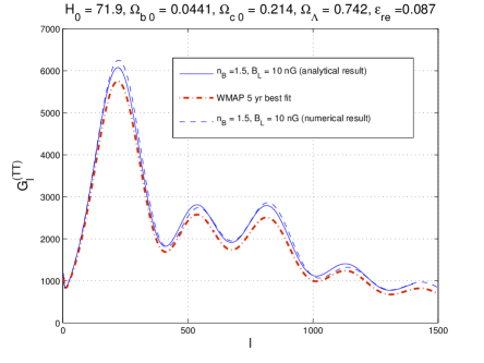
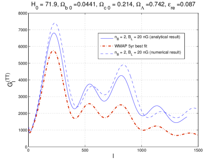
Figure 4: The temperature autocorrelations are illustrated in the case of rather large values of the magnetic field (i.e. $10$ and $20$ nG) with the purpose of emphasizing the typical patterns of distortions induced by the magnetized adiabatic mode of Eq. (3.78). For comparison the WMAP-5y best fit has been also included. These plots as the following ones are adapted from Ref. [153].

In Fig. 4 we illustrate the $TT$ autocorrelations for a deliberately extreme set of parameters: this choice will make more apparent the effect of the increase of the magnetic field intensity. The inclusion of a magnetized background has a threefold effect on the temperature autocorrelations: the height of the first acoustic peak increases, the second peak is distorted and it eventually turns into a hump for sufficiently large values of $B_{\mathrm{L}}$ (or of $n_{\mathrm{B}}$). The third peak is, at the same time, distorted and raised. In Fig. 4 as we move from the plot at the left to the plot at the right the spectral index increases. The increase of the spectral slope entails also an increase of the distortions, as we can see from Fig. 4.

As suggested in [153, 154] the impact of the magnetic field parameters follows from the relative ratios of the first three acoustic peaks which defined as:

$$\overline{H}_{1}=\frac{{\mathcal{G}}^{(\mathrm{TT})}_{\ell_{1}}}{{\mathcal{G}}^{(\mathrm{TT})}_{\ell=10}}\qquad\overline{H}_{2}=\frac{{\mathcal{G}}^{(\mathrm{TT})}_{\ell_{2}}}{{\mathcal{G}}^{(\mathrm{TT})}_{\ell_{1}}},\qquad\overline{H}_{3}=\frac{{\mathcal{G}}^{(\mathrm{TT})}_{\ell_{3}}}{{\mathcal{G}}^{(\mathrm{TT})}_{\ell_{2}}},$$ (4.28)

where $\ell_{1}={\mathcal{O}}(220)$, $\ell_{2}={\mathcal{O}}(535)$ and $\ell_{3}={\mathcal{O}}(816)$ are, respectively, the locations of the first three acoustic peaks. When the magnetic field intensity increases we have that, typically, $\overline{H}_{1}$ and $\overline{H}_{3}$ increase more than $\overline{H}_{2}$ so that the resulting shape of the $TT$ correlations changes qualitatively.

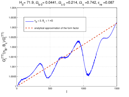
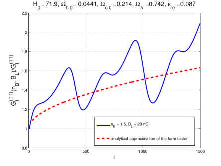
Figure 5: The scaling properties of the magnetized $TT$ correlations.

To gauge the effects of the magnetic random fields on the $TT$ correlations a practical strategy is to fix the $\Lambda$CDM parameters to their best-fit values and then construct the ratio ${\mathcal{G}}^{(\mathrm{TT})}(n_{\mathrm{B}},B_{\mathrm{L}})/{\mathcal{G}}^{(\mathrm{TT})}$ where ${\mathcal{G}}^{(\mathrm{TT})}(n_{\mathrm{B}},B_{\mathrm{L}})$ is the angular power spectrum computed for a particular set of parameters of the magnetized background and ${\mathcal{G}}^{(\mathrm{TT})}$ is the angular power spectrum for the best fit of the $\Lambda$CDM parameters. In Fig. 5 this ratio is illustrated for different values of the intensity and of the spectral index. What is apparent is that a magnetic field $B_{\mathrm{L}}={\mathcal{O}}(1)$ nG induces a modification ${\mathcal{O}}(10^{-3})$ on the shape of the angular power spectrum (see [153] for further details).

The dashed lines in Fig. 5 and the full lines in Fig. 4 illustrate the results of the analytic approximation to the temperature autocorrelations. The idea, in short, is to include consistently the contributions of the magnetic fields in the evolution of the monopole and of the dipole of the brightness perturbations and to evaluate the angular power spectra by using a semi-analytic form of the visibility function (like the one outlined in Eq. (4.6)). Assuming tight coupling between photons, electrons and baryons, the evolution of the monopole and of the dipole of the brightness perturbations determines the source term in the temperature and polarization anisotropies. The monopole and the dipole obey, in Fourier space, the following pair of equations:

$$(\psi-\Delta_{\mathrm{I}0})^{\prime}=k\Delta_{\mathrm{I}1},$$ (4.29)

$$[(R_{\mathrm{b}}+1)\Delta_{\mathrm{I}1}]^{\prime}+2\frac{k^{2}}{k_{\mathrm{D}}^{2}}(R_{\mathrm{b}}+1)\Delta_{\mathrm{I}1}=\frac{k}{3}\Delta_{\mathrm{I}0}+\frac{k(R_{\mathrm{b}}+1)}{3}\phi+\frac{k(\Omega_{\mathrm{B}}-4\sigma_{\mathrm{B}})}{12},$$ (4.30)

where $k_{\mathrm{D}}$ is the wave-number corresponding to diffusive damping.To lowest-order in the photon-baryon coupling the diffusive damping is $k_{\mathrm{D}}^{-2}=\eta/[\rho_{\gamma}(1+R_{\mathrm{b}})]$ where $\eta$ has been defined right after Eq. (3.20); more precisely we have [49, 103, 105]:

$$\frac{1}{k^{2}_{\mathrm{D}}}=\frac{2}{5}\int_{0}^{\tau}c_{\mathrm{sb}}(\tau^{\prime})\frac{a_{0}d\tau^{\prime}}{a(\tau^{\prime})\,\,x_{\mathrm{e}}n_{\mathrm{e}}\sigma_{\mathrm{e}\gamma}}.$$ (4.31)

The estimates based on shear viscosity can be improved by going to higher order in the tight-coupling expansion and by further refining the estimates depending upon the explicit values of the $\Lambda$CDM parameters. To second order in the tight-coupling expansion the inclusion of the polarization allows one to estimate [107, 108]:

$$\frac{1}{k_{\mathrm{D}}^{2}}=\int_{0}^{\tau}\frac{d\tau^{\prime}}{6(R_{\mathrm{b}}+1)\epsilon^{\prime}}\biggl{[}\frac{16}{15}+\frac{R_{\mathrm{b}}^{2}}{R_{\mathrm{b}}+1}\biggr{]}.$$ (4.32)

The factor $16/15$ arises since the polarization fluctuations are taken consistently into account in the derivation. This difference is physically relevant. Grossly speaking we can indeed say that more polarization implies more anisotropy (and vice versa); more polarization implies a faster damping by diffusion. Note that $k_{\mathrm{D}}$ provides an effective ultra-violet cut-off for the magnetic energy spectra and will be used later on.

The evolution of the monopole and of the dipole can be determined from the WKB solution of Eqs. (4.29) and (4.30), i.e.

$$\Delta_{\mathrm{I}0}(k,\tau)+\phi(k,\tau)={\mathcal{L}}(k,\tau)+\sqrt{c_{\mathrm{sb}}}{\mathcal{M}}(k,\tau)\cos{[kr_{\mathrm{s}}(\tau)]}\,e^{-\frac{k^{2}}{k_{\mathrm{D}}^{2}}},$$ (4.33)

$$\Delta_{\mathrm{I}1}(k,\tau)=c_{\mathrm{sb}}^{3/2}{\mathcal{M}}(k,\tau)\sin{[k\,r_{\mathrm{s}}(\tau)]}e^{-\frac{k^{2}}{k_{\mathrm{D}}^{2}}},$$ (4.34)

where ${\mathcal{L}}(k,\tau)$ and ${\mathcal{M}}(k,\tau)$ are fixed once the initial conditions of the Einstein-Boltzmann hierarchy are specified. In what follows, as already mentioned, the initial conditions shall correspond to the magnetized adiabatic mode. More details on the semi-analytic approaches for the analysis of the temperature and polarization anisotropies can be found in a series of papers [136, 153].

The coefficients $a_{\ell m}^{(\mathrm{T})}$ and $a_{\ell m}^{(\mathrm{E})}$ are determined in terms of the monopole, dipole and quadrupole of the intensity and in terms of the monopole and quadrupole of the polarization. More specifically the coefficient $a_{\ell m}^{(\mathrm{T})}$ is

$$a^{(\mathrm{T})}_{\ell m}=\frac{\sqrt{4\pi}}{(2\pi)^{3/2}}\,(-i)^{\ell}\,\sqrt{2\ell+1}\int d^{3}ke^{-\frac{k^{2}}{k_{\mathrm{t}}^{2}}}\biggl{[}(\Delta_{\mathrm{I}0}+\phi)j_{\ell}(x)+3\Delta_{\mathrm{I}1}\biggl{(}\frac{dj_{\ell}}{dx}\biggr{)}\biggr{]},$$ (4.35)

where $x=k(\tau_{0}-\tau_{*})$ and where $j_{\ell}(x)$ are the spherical Bessel functions [159, 160] of argument $x$. In Eq. (4.35) $k_{\mathrm{t}}=\sqrt{3}/\sigma_{*}$ arises from the integration over $\tau$ of the Gaussian visibility function. The coefficient $a_{\ell m}^{(\mathrm{E})}$ turns out to be:

$$a_{\ell m}^{(\mathrm{E})}=\frac{3}{4}\frac{(-i)^{\ell}}{(2\pi)^{3/2}}\sqrt{\frac{(\ell-2)!}{(\ell+2)!}}\sqrt{4\pi}\sqrt{2\ell+1}\int d^{3}k\,\,x^{2}\,\,[(1+\partial_{x}^{2})^{2}]j_{\ell}(x)\int_{0}^{\tau_{0}}{\mathcal{K}}(\tau)S_{\mathrm{P}}(k,\tau)d\tau.$$ (4.36)

Using Eqs. (4.35) and (4.36) in Eqs. (4.20), (4.25) and (4.26) we can obtain the semianalytic forms of the $TT$, $TE$ and $EE$ angular power spectra. This is the way the dashed lines in Fig. 5 have been computed. As we shall see the same approximations lead to some interesting results for the $TE$ and $EE$ correlations.

4.5 Magnetized polarisation correlations and cross-correlations

The $TE$ cross-correlations together with the $TT$ spectra are among the most useful indicators of the adiabatic nature of the CMB initial conditions. The polarization observations are therefore a rather sensitive tool which can be used for the scrutiny of a magnetized component.

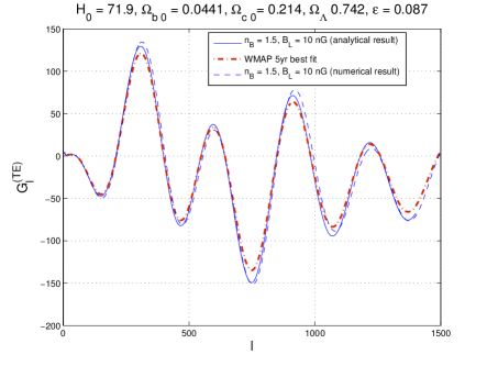
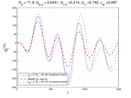
Figure 6: The $TE$ correlations are illustrated for the same set of extreme magnetic field parameters already employed in Fig. 5. In both plots with the full lines we reported the analytical results obtained on the basis of the approximation scheme mentioned in Eqs. (4.33) and (4.34).

In Fig. 6 the $TE$ correlations are illustrated for the case of blue magnetic spectral indices $1<n_{\mathrm{B}}<5/2$. On a purely qualitative ground when the magnetic field is of the order of $0.1$ nG the magnetized TE correlations cannot be distinguished from the angular power spectra computed in the absence of magnetic fields. This observation shows once more the typical sensitivities of this type of approach.

Unlike the case of the temperature autocorrelations (where the position of the Doppler peak cannot be moved by a stochastic magnetic field) there is an observable shift of the second and third (correlation) peaks of the $TE$ spectra. This distortion also entails a shift of the position of the corresponding peaks. A similar effect is observed in the magnetized $EE$ correlations which are reported in Fig. 7 (see in particular the plot at the right).

Figures 6 and 7 show, a posteriori, that the magnetic fields also affect the polarization observables even without a Faraday rotation term (which will be specifically discussed in section 5). The physical reason of the obtained result can be easily understood: to zeroth-order in the tight-coupling expansion, the magnetic field affects the dipole of the brightness perturbation for the intensity. Always to zeroth order, this contribution is reflected in a further source term for the monopole. But both the $TE$ and $EE$ power spectra arise to first-order in the tight-coupling expansion and are proportional to the first-order dipole through a term which is, up to a numerical factor, $k/\epsilon^{\prime}$. This shows why we also get an effect on the polarization observables even if the Faraday rotation term is absent.

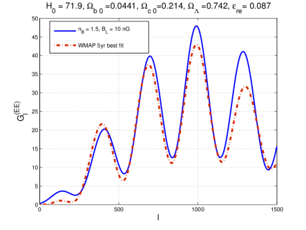
Figure 7: The $EE$ correlations are illustrated for the same sets of parameters of Figs. 5 and 6. Note that in the left plot, with the dashed line, we illustrate the semi-analytic approximation in the absence of magnetic fields.

The results illustrated in this section show that it is possible to obtain accurate estimates of the temperature autocorrelations and of the polarization correlations also in the presence of a magnetized background.

5 Faraday rotation

In a magnetized plasma the linear polarization of the microwave background rotates thanks to the Faraday effect and this suggestion already appeared in a relevant remark of Ref. [53] where the author argued that repeated Thomson scatterings of the primeval radiation during the early phases of a slightly anisotropic universe would modify the black-body spectrum and produce linear polarization. The CMB polarization could then be modified by the depolarizing effect of a uniform magnetic field [53] possibly accommodated in an axisymmetric background geometry. After the first observations of the temperature anisotropies, the Faraday rotation of the microwave background has been analyzed in different frameworks [200, 201, 202]. By developing the original perspective of Ref. [53] the initial analyses have been conducted within the uniform field approximation [200, 201, 202] (see also [203]). In the case of magnetic random fields the Faraday rotation is however characterized by a specific power spectrum [204] (see also [205, 206, 207]) and the uniform field approximation is not always suitable. The Faraday effect may also mix with the birefringence induced by pseudo-scalar particles [207] (see also [208, 209]). In this case the frequency dependence of the signal differs from the situation of the Faraday effect alone. From the viewpoint of the temperature and polarization angular power spectra the Faraday effect rotates the $E$-mode polarization into a $B$-mode that must be computed from the appropriate magnetized initial conditions [210] already introduced in the previous section. In this case the total $B$-mode polarization will be a convolution of the Faraday rotation spectrum and of the $E$-mode autocorrelation determined, in its turn, by the magnetized initial conditions explored in sections 3 and 4. In a more realistic perspective the Faraday rotation occurs while the polarization is formed without an explicit scale separation between the two moments; the theoretical analysis of this description is still not completely clear.

5.1 Pivotal frequencies

Since the Faraday effect leads to a frequency-dependent $B$-mode power spectrum it is sometimes relevant to define a pivot frequency at which the signal is computed. This possible need of a pivotal frequency scale is rarely mentioned in the current literature and it is therefore useful to clarify this aspect. The energy density of the CMB spectrum in critical units can be written as

$$\frac{1}{\rho_{\mathrm{c}}}\frac{d\rho_{\gamma}}{d\ln{\overline{\omega}}}=\frac{15}{\pi^{4}}h_{0}^{2}\Omega_{\gamma 0}\,g(x),\qquad h_{0}^{2}\Omega_{\gamma 0}=2.47\times 10^{-5},$$ (5.1)

where $g(x)=x^{4}/(e^{x}-1)$; note that $x=\overline{\omega}/T_{\gamma 0}$ and $\overline{\omega}=2\pi\overline{\nu}$. The maximum of the spectral energy density (5.1) follows from the extremum of $g(x)$ and the result is $x_{\mathrm{max}}^{(\rho)}=3.920$. In analog terms the maximum of the brightness of the microwave background spectrum follows from the extremum of $f(x)=x^{3}/(e^{x}-1)$ corresponding to $x_{\mathrm{max}}^{(b)}=2.821$. Consequently, two motivated pivotal frequencies for the normalization of the $B$-mode autocorrelation induced by the Faraday effect are, respectively, the maximum of the brightness and of the energy density

$$\overline{\nu}^{(b)}_{\mathrm{max}}=160.3\,\mathrm{GHz},\qquad\overline{\nu}^{(\rho)}_{\mathrm{max}}=222.6\,\mathrm{GHz},$$ (5.2)

where $\overline{\nu}^{(b)}$ and $\overline{\nu}_{\mathrm{max}}$ denote respectively the maximum of the brightness and of the spectral energy density. When needed, we shall preferentially use $\overline{\nu}^{(\rho)}_{\mathrm{max}}$ as pivotal frequency for the Faraday rotation signal.

The rationale for the introduction of the pivot frequency also depends on the widely different observational channels exploited by the various experiments. For instance the WMAP experiment observed the microwave sky in five frequency channels centered at $23$, $33$, $41$, $61$ and $94$ in units of GHz. The Planck experiment observed the microwave sky in nine frequency channels: three frequency channels (i.e. $30,\,44,\,70$ GHz) belonged to the low frequency instrument (LFI); six channels (i.e. $100,\,143,\,217,\,353,\,545,\,857$ GHz) belonged to the high frequency instrument (HFI). Since not all the channels see the same $B$-mode angular power spectrum it is desirable that observational papers would clearly specify the pivot frequency when comparing their results to potential theoretical signals coming from the Faraday effect. This is rarely done since, understandably, each collaboration just considers its own operating frequency (for instance $70$ GHz in the case of Ref. [89] or $148$ GHz in the case of Ref. [102]). We point out that this practice can be improved by referring the angular power spectra either to the maximum of the spectral energy density or to the maximum of the brightness, as suggested in Eq. (5.2).

5.2 Dispersion relations

When the frequency of the (polarized) CMB photons exceeds the plasma frequency the baryon fluid is no longer a sound dynamical approximation and a two-fluid description is mandatory. This is the essence of Faraday rotation and of the other dispersive phenomena that can be analyzed by studying the propagation of high-frequency waves in magnetized plasmas.

The relevant dispersion relations are derived by linearizing Eqs. (2.19)–(2.20) in the presence of a background magnetic field $\vec{B}(\vec{x})$. By separating the background fields from the propagating electromagnetic waves we have

$$n_{\rm e,\,i}(\vec{x},\tau)=n_{0}+\delta n_{\rm e,\,i}(\vec{x},\tau),\qquad\vec{B}(\vec{x},\tau)=\vec{B}(\vec{x})+\vec{b}(\vec{x},\tau),$$

$$\vec{v}_{\rm e,\,i}(\vec{x},\tau)=\delta\vec{v}_{\rm e,\,i}(\vec{x},\tau),\qquad\vec{E}(\vec{x},\tau)=\vec{e}(\vec{x},\tau),$$ (5.3)

where $\vec{e}(\vec{x},\tau)$ and $\vec{b}(\vec{x},\tau)$ are, respectively, the electric and magnetic fields of the wave while $\vec{B}(\vec{x})$ is the large-scale magnetic random field. The evolution of the concentrations and of the velocities for electrons and ions

$$\delta n_{\rm e}^{\,\prime}+n_{0}\vec{\nabla}\cdot\delta\vec{v}_{\rm e}=0,\qquad\delta\vec{v}_{\rm e}^{\,\prime}+{\cal H}\delta\vec{v}_{\rm e}=-\frac{e}{m_{\rm e}a}\biggl{[}\vec{e}+\delta\vec{v_{\rm e}}\times\vec{B}\biggr{]},$$ (5.4)

$$\delta n_{\rm i}^{\,\prime}+n_{0}\vec{\nabla}\cdot\delta\vec{v}_{\rm i}=0,\qquad\delta\vec{v}_{\rm i}^{\,\prime}+{\cal H}\delta\vec{v}_{\rm i}=\frac{e}{m_{\rm i}a}\biggl{[}\vec{e}+\delta\vec{v_{\rm i}}\times\vec{B}\biggr{]},$$ (5.5)

can be used to solve for the propagation of the electromagnetic waves in the plasma by using the following pair of equations:

$$\vec{\nabla}\times\vec{e}=-\vec{b}^{\,\,\prime},\qquad\vec{\nabla}\times\vec{b}=\vec{e}^{\,\,\prime}+4\pi\,e\,n_{0}(\delta\vec{v}_{\rm i}-\delta\vec{v}_{\rm e}),$$ (5.6)

by recalling that the corresponding electric and magnetic fields are both divergenceless (i.e. $\vec{\nabla}\cdot\vec{e}=0$ and $\vec{\nabla}\cdot\vec{b}=0$).

Waves that are locally parallel (i.e. $\parallel$) or orthogonal (i.e. $\perp$) to the magnetic field $\vec{B}$ obey different dispersion relations. As already mentioned in connection with the plasma hierarchies, the trajectory of the charged species can be determined as a perturbation around the centre of the particle orbit [60, 61] by using an expansion of the magnetic random field in spatial gradients and by keeping the leading order result. In the present context the magnetic field is uniform over the typical scale of the particle orbit, which also means that the field experienced by the electron in traversing a Larmor orbit is almost constant. By taking the Fourier and the Laplace transforms the evolution equations (5.6) can be recast in the following form

$$k^{2}\vec{e}_{\vec{k},\overline{\omega}}-(\vec{k}\cdot\vec{e}_{\vec{k},\overline{\omega}})\vec{k}=\epsilon(\overline{\omega},\alpha)\overline{\omega}^{2}\vec{e}_{\vec{k},\overline{\omega}},\qquad\alpha=i{\mathcal{H}}/\overline{\omega}=H/\omega\ll 1,$$ (5.7)

where $\alpha$ accounts for the curved-space corrections. The dielectric tensor $\epsilon(\overline{\omega},\alpha)$ can be written in a generalized matrix notation as:

$$\epsilon(\overline{\omega},\alpha)=\left(\matrix{\epsilon_{\perp 1}(\overline{\omega},\alpha)&i\epsilon_{\perp 2}(\overline{\omega},\alpha)&0&\cr-i\epsilon_{\perp 2}(\overline{\omega},\alpha)&\epsilon_{\perp 1}(\overline{\omega},\alpha)&0&\cr 0&0&\epsilon_{\parallel}(\overline{\omega},\alpha)}\right),$$ (5.8)

where the various entries of the matrix (5.8) are:

$$\epsilon_{\parallel}(\overline{\omega},\alpha)=1-\frac{\overline{\omega}_{\rm p\,i}^{2}}{\overline{\omega}^{2}(1+\alpha)}-\frac{\overline{\omega}_{\rm p\,e}^{2}}{\overline{\omega}^{2}(1+\alpha)},$$ (5.9)

$$\epsilon_{\perp 1}(\overline{\omega},\alpha)=1-\frac{\overline{\omega}^{2}_{\rm p\,i}(\alpha+1)}{\overline{\omega}^{2}(\alpha+1)^{2}-\overline{\omega}_{\rm B\,i}^{2}}-\frac{\overline{\omega}^{2}_{\rm p\,e}(\alpha+1)}{\overline{\omega}^{2}(\alpha+1)^{2}-\overline{\omega}_{\rm B\,e}^{2}},$$ (5.10)

$$\epsilon_{\perp 2}(\omega,\alpha)=\frac{\overline{\omega}_{\rm B\,e}}{\overline{\omega}}\frac{\overline{\omega}^{2}_{\rm p\,e}}{\overline{\omega}^{2}(\alpha+1)^{2}-\overline{\omega}^{2}_{\rm B\,e}}-\frac{\overline{\omega}_{\rm B\,i}}{\overline{\omega}}\frac{\overline{\omega}^{2}_{\rm p\,i}}{\overline{\omega}^{2}(\alpha+1)^{2}-\overline{\omega}^{2}_{\rm B\,i}}.$$ (5.11)

Introducing now $\vec{k}_{\parallel}=k\cos{\vartheta}$ and $\vec{k}_{\perp}=k\sin{\vartheta}$, the relevant dispersion relations are readily deduced from Eq. (5.7):

$$2\epsilon_{\parallel}\cos^{2}{\theta}[(n^{2}-\epsilon_{-})(n^{2}-\epsilon_{+})]=\sin^{2}{\theta}(\epsilon_{\parallel}-n^{2})[n^{2}(\epsilon_{+}+\epsilon_{-})-2\epsilon_{+}\epsilon_{-}].$$ (5.12)

In Eq. (5.12), as usual, the refractive index is defined as $\overline{\omega}/k=1/n$. Equation (5.12) is the Appleton-Hartree dispersion relation [56, 57] and $\epsilon_{\pm}(\omega,\alpha)=\epsilon_{\perp 1}(\omega,\alpha)\pm\epsilon_{\perp 2}(\omega,\alpha)$ are the dielectric tensors in the circular basis.

If the propagation occurs along the magnetic field direction [i.e. $\theta=0$ in Eq. (5.12)] the waves with positive helicity (i.e. $\hat{e}_{+}$) and negative helicity (i.e. $\hat{e}_{-}$) experience two different phase velocities $v_{\pm}(\omega,\alpha)=1/n_{\pm}(\overline{\omega},\alpha)$ with $n_{\pm}(\overline{\omega},\alpha)=\sqrt{\epsilon_{\pm}(\overline{\omega},\alpha)}$. Conversely when the propagation is orthogonal to the magnetic field direction there is an ordinary and an extraordinary wave whose dispersion relations are given, respectively, by

$$k_{\mathrm{O}}=\overline{\omega}\sqrt{1-\frac{\overline{\omega}_{\mathrm{pe}}^{2}}{\overline{\omega}^{2}(1+\alpha)}},$$ (5.13)

$$k_{\mathrm{E}}=\overline{\omega}\sqrt{\frac{\overline{\omega}[\overline{\omega}^{2}(\alpha+1)^{2}-\overline{\omega}_{\mathrm{Be}}^{2}]-2\overline{\omega}_{\mathrm{pe}}^{2}\overline{\omega}^{2}(\alpha+1)+\overline{\omega}_{\mathrm{pe}}^{4}}{\overline{\omega}^{2}[\overline{\omega}^{2}(\alpha+1)^{2}-\overline{\omega}_{\mathrm{Be}}^{2}-\overline{\omega}_{\mathrm{pe}}^{2}(\alpha+1)]}}.$$ (5.14)

Equations (5.13) and (5.14) imply, in the physical range of frequencies, that $\overline{\omega}^{2}\to k^{2}$. The typical CMB angular frequency of Eq. (5.2) is actually ${\mathcal{O}}(200)$ GHz and hence much larger than the plasma and Larmor frequencies (see Eqs. (2.27)–(2.28)) which are instead in the MHz or even kHz ranges. Furthermore, in the physical range of parameters the plasma and Larmor frequencies of the electrons are always much larger than the corresponding frequencies of the ions. Thus the relevant physical regime of the dispersion relations can be summarized by the following hierarchies between the various frequencies:

$$\frac{\overline{\omega}_{\mathrm{pe}}}{\overline{\omega}_{\mathrm{Be}}}\gg 1,\qquad\frac{\overline{\omega}_{\mathrm{pi}}}{\overline{\omega}_{\mathrm{Bi}}}\gg 1,\qquad\frac{\overline{\omega}_{\mathrm{pe}}}{\overline{\omega}_{\mathrm{pi}}}\gg 1,\qquad\frac{\overline{\omega}}{\overline{\omega}_{\mathrm{pe}}}\gg 1,$$ (5.15)

where, as already mentioned, $\overline{\omega}$ denotes the comoving angular frequency of the microwave background photons estimated, for instance, from the maximum of the spectral energy density (see Eq. (5.2)). Under the conditions expressed by Eq. (5.15) the expressions of $\epsilon_{\pm}(\overline{\omega},\alpha)$ greatly simplifies and the result is

$$\epsilon_{\pm}(\overline{\omega},\alpha)=1-\frac{\overline{\omega}_{\mathrm{pe}}^{2}}{\overline{\omega}[\overline{\omega}(\alpha+1)\pm\overline{\omega}_{\mathrm{Be}}]},$$ (5.16)

implying that the dispersion relations of the ordinary and extraordinary wave are $\overline{\omega}^{2}\to k^{2}$, as it follows also in different plasmas [57].

5.3 Microwave background polarization and Faraday screening

For a monochromatic wave polarized along $\hat{e}_{1}$ at $\tau=0$ (e.g. $\vec{e}(z,\tau)=E_{0}\hat{e}_{1}e^{-i(\overline{\omega}\tau-kz)}$) the positive and negative helicities are defined as $\hat{e}_{\pm}=(\hat{e}_{1}\pm i\hat{e}_{2})/\sqrt{2}$. Consequently the linear polarization is effectively composed by two circularly polarized waves, one with positive helicity (propagating with wavenumber $k_{+}=\sqrt{\epsilon_{+}(\overline{\omega},\alpha)}\,\,\overline{\omega}$) the other with negative helicity (propagating with wavenumber $k_{-}=\sqrt{\epsilon_{-}(\overline{\omega},\alpha)}\,\,\overline{\omega}$). We have therefore that after a conformal time $\tau$ the electric field of the wave will be

$$\vec{e}(z,\tau) = \frac{E_{0}}{\sqrt{2}}\biggl{[}\hat{e}_{+}e^{-i(\overline{\omega}\tau-k_{+}z)}+\hat{e}_{-}e^{-i(\overline{\omega}\tau-k_{+}z)}\biggr{]}$$ (5.17)

$$= \frac{E_{0}}{2}\biggl{[}\hat{e}_{1}\biggl{(}e^{ik_{+}z}+e^{ik_{-}z}\biggr{)}+i\hat{e}_{2}\biggl{(}e^{ik_{+}z}-e^{ik_{-}z}\biggr{)}\biggl{]}e^{-i\overline{\omega}\tau},$$

where the second equality follows from the definitions of $\hat{e}_{\pm}$. We can now compute easily the four Stokes parameters of the wave which are, by definition,

$$I=|\vec{e}\cdot\hat{e}_{1}|^{2}+|\vec{e}\cdot\hat{e}_{2}|^{2},\qquad V=2\,\mathrm{Im}[(\vec{e}\cdot\hat{e}_{1})^{*}(\vec{e}\cdot\hat{e}_{2})],$$ (5.18)

$$Q=|\vec{e}\cdot\hat{e}_{1}|^{2}-|\vec{e}\cdot\hat{e}_{2}|^{2},\qquad U=2\,\mathrm{Re}[(\vec{e}\cdot\hat{e}_{1})^{*}(\vec{e}\cdot\hat{e}_{2})].$$ (5.19)

When the polarization plane of the incoming wave is rotated, two out of four Stokes parameter will be rotated; more specifically while $I$ and $V$ are left invariant, $Q$ and $U$ are rotated. Inserting Eq. (5.17) into Eqs. (5.18) and (5.19) the only Faraday rotated Stokes parameters are:

$$Q^{(\mathrm{F})}=Q^{(\mathrm{in})}\cos{(2\Delta\Phi)}+U^{(\mathrm{in})}\sin{(2\Delta\Phi)},$$

$$U^{(\mathrm{F})}=-Q^{(\mathrm{in})}\sin{(2\Delta\Phi)}+U^{(\mathrm{in})}\cos{(2\Delta\Phi)}.$$ (5.20)

where, by definition,

$$\Delta\Phi=\frac{\overline{\omega}}{2}\biggl{[}\sqrt{\epsilon_{+}(\overline{\omega},\alpha)}-\sqrt{\epsilon_{-}(\overline{\omega},\alpha)}\biggr{]}\Delta z.$$ (5.21)

The rate of rotation per unit time is called Faraday rotation rate and it is given by:

$${\mathcal{F}}(\hat{n}) = \frac{d\Phi}{d\tau}=\frac{\overline{\omega}}{2}\biggl{[}\sqrt{\epsilon_{+}(\overline{\omega},\alpha)}-\sqrt{\epsilon_{-}(\overline{\omega},\alpha)}\biggr{]}$$

$$= \frac{\overline{\omega}_{\mathrm{Be}}}{2}\biggl{(}\frac{\overline{\omega}_{\mathrm{pe}}}{\overline{\omega}}\biggl{)}^{2}\equiv\frac{e^{3}}{2\pi m_{\mathrm{e}}^{2}}a\tilde{n}_{\mathrm{e}}x_{\mathrm{e}}\biggl{(}\frac{\vec{B}\cdot\hat{n}}{\overline{\nu}^{2}}\biggr{)},$$

$$\mathrm{F}(\hat{n}) = \frac{{\mathcal{F}}(\hat{n})}{\epsilon^{\prime}}=\frac{3}{16\pi^{2}e}\frac{\hat{n}\cdot\vec{B}}{\overline{\nu}^{2}}.$$ (5.22)

The first line of Eq. (5.22) is the definition of Faraday rotation rate; the second line of Eq. (5.22) follows by recalling the hierarchies of Eq. (5.15) i.e. $|\overline{\omega}/\overline{\omega}_{\mathrm{pe}}|\gg 1$ and for $|\overline{\omega}/\overline{\omega}_{\mathrm{Be}}|\gg 1$. Finally, the third line of Eq. (5.22) follows by taking into account the definition of the differential optical depth, (i.e. $\epsilon^{\prime}=a\tilde{n}_{\mathrm{e}}x_{\mathrm{e}}\sigma_{\mathrm{e}\gamma}$) and by making the cross section of Eq. (2.58) explicit.

In the conventional lore the polarization is only generated very near the surface of last scattering as the photons begin to decouple from the electrons and generate a quadrupole moment through free-streaming [200, 201, 202]. According to this perspective the polarization of the microwave background is first generated and then it is rotated by a Faraday screen. From Eqs. (5.20) and (5.22) we can take the total time derivative supposing that the initial polarization is independent on time. From the Faraday rotation rate we then get:

$$\Delta_{\mathrm{Q}}^{\prime}+n^{i}\partial_{i}\Delta_{\mathrm{Q}}=2\epsilon^{\prime}F(\hat{n})\Delta_{\mathrm{U}},\qquad\Delta_{\mathrm{U}}^{\prime}+n^{i}\partial_{i}\Delta_{\mathrm{U}}=-2\epsilon^{\prime}F(\hat{n})\Delta_{\mathrm{Q}}.$$ (5.23)

Even if the polarization and its rotation are two concurrent phenomena, the approximation of the Faraday screening is considered satisfactory as long as the Faraday rotation rate is sufficiently small. Equations (5.23) describe the Faraday rotation mixing which can be computed within two complementary strategies. In the first approach the $E$-mode polarization is computed as if the magnetic fields were absent from the initial conditions of the Einstein-Boltzmann hierarchy (see e.g. [200, 201, 202, 203, 206, 211, 212]). In a more realistic strategy the $E$-mode polarization is computed by taking into account the appropriate magnetized initial conditions [210]. While within the first approach the calculation just assumes the conventional adiabatic mode of the concordance paradigm, in the second approach the magnetic random fields not only affect the Faraday rotation rate but also the $E$-mode power spectrum. The total angle of rotation at some reference time $\tau=\tau_{*}$ is defined in terms of the visibility function of Eq. (4.5):

$$\Phi(\hat{n},\tau_{*})={\mathcal{A}}(\overline{\nu})\int_{0}^{\tau_{*}}{\mathcal{K}}(\tau)\,[\hat{n}\cdot\vec{B}(\vec{x},\tau)]\,\,d\tau,\qquad{\mathcal{K}}(\tau)=\epsilon^{\prime}(\tau)e^{-\epsilon(\tau,\tau_{*})}.$$ (5.24)

where ${\mathcal{A}}(\overline{\nu})=3/(16\pi^{2}e\overline{\nu}^{2})$ depends upon the comoving frequency $\overline{\nu}$. Given an explicit form of the visibility function (see e.g. Eqs. (4.7)) the total rotation rate can be approximately evaluated [205, 210]. In the sudden approximation the visibility function is sharply peaked around the decoupling time with practically zero width so that, in this limit, $\Phi(\hat{n},\tau_{*})\to F(\hat{n},\tau_{*})$.

5.4 Induced $B$-mode polarization

The $B$-mode polarization induced by the Faraday rate is more easily estimated in real space; the angular power spectrum is obtained after a simple but lengthy algebra. The starting point of the derivation are the two orthogonal combinations of the brightness perturbations already introduced in Eq. (4.22), namely $\Delta_{\pm}(\hat{n},\tau)=\Delta_{\mathrm{Q}}(\hat{n},\tau)\pm i\Delta_{\mathrm{U}}(\hat{n},\tau)$; in terms of these quantities the $E$-mode and the $B$-mode polarizations are given by:

$$\Delta_{\mathrm{E}}(\hat{n},\tau) = -\frac{1}{2}\biggl{\{}(1-\mu^{2})\partial_{\mu}^{2}(\Delta_{+}+\Delta_{-})-4\mu\partial_{\mu}(\Delta_{+}+\Delta_{-})-2(\Delta_{+}+\Delta_{-})$$ (5.25)

$$- \frac{\partial_{\varphi}^{2}(\Delta_{+}+\Delta_{-})}{1-\mu^{2}}+2i\biggl{[}\partial_{\varphi}\partial_{\mu}(\Delta_{+}-\Delta_{-})-\frac{\mu}{1-\mu^{2}}\partial_{\varphi}(\Delta_{+}-\Delta_{-})\biggr{]}\biggr{\}},$$

$$\Delta_{\mathrm{B}}(\hat{n},\tau) = \frac{i}{2}\biggl{\{}(1-\mu^{2})\partial_{\mu}^{2}(\Delta_{+}-\Delta_{-})-4\mu\partial_{\mu}(\Delta_{+}-\Delta_{-})-2(\Delta_{+}-\Delta_{-})$$ (5.26)

$$- \frac{\partial_{\varphi}^{2}(\Delta_{+}-\Delta_{-})}{1-\mu^{2}}+2i\biggl{[}\partial_{\varphi}\partial_{\mu}(\Delta_{+}+\Delta_{-})-\frac{\mu}{1-\mu^{2}}\partial_{\varphi}(\Delta_{+}+\Delta_{-})\biggr{]}\biggr{\}},$$

where, as usual, $\partial_{\mu}$ denotes a derivation with respect to $\mu=\cos{\vartheta}$ while $\partial_{\varphi}$ denotes a derivation with respect to $\varphi$. According to Eqs. (5.25) and (5.26) the initial B-mode polarization is absent (i.e. $\Delta_{\mathrm{B}}(\hat{n},\tau)=0$) provided $\Delta_{+}(\hat{n},\tau)=\Delta_{-}(\hat{n},\tau)$ and when the brightness perturbation does not depend on $\varphi$ [i.e. $\partial_{\varphi}(\Delta_{+}+\Delta_{-})=0$]. Once $\Delta_{\mathrm{E}}(\hat{n},\tau)$ and $\Delta_{\mathrm{B}}(\hat{n},\tau)$ are determined, it is sufficient to recall that:

$$a^{(\mathrm{E})}_{\ell\,m}=N_{\ell}\int d\hat{n}\,\Delta_{\mathrm{E}}(\hat{n},\tau)\,Y^{*}_{\ell\,m}(\hat{n}),\qquad a^{(\mathrm{B})}_{\ell\,m}=N_{\ell}\int d\hat{n}\,\Delta_{\mathrm{B}}(\hat{n},\tau)\,Y^{*}_{\ell\,m}(\hat{n}),$$ (5.27)

where $N_{\ell}=\sqrt{(\ell-2)!/(\ell+2)!}$. In terms of Eq. (5.27) the $EE$ and $BB$ angular power spectra can be easily computed from their definition:

$$C_{\ell}^{(\mathrm{EE})}=\frac{1}{2\ell+1}\sum_{m=-\ell}^{\ell}\langle a^{(\mathrm{E})*}_{\ell m}\,a^{(\mathrm{E})}_{\ell m}\rangle,\qquad C_{\ell}^{(\mathrm{BB})}=\frac{1}{2\ell+1}\sum_{m=-\ell}^{\ell}\langle a^{(\mathrm{B})*}_{\ell m}\,a^{(\mathrm{B})}_{\ell m}\rangle,$$ (5.28)

where, as usual, $\langle...\rangle$ denotes the ensemble average. If the Faraday rate operates after the linear polarization is effectively produced, to lowest order in the rate the $E$-mode and the $B$-mode in real space are, respectively,

$$\Delta_{\mathrm{E}}(\hat{n},\tau) = -\partial_{\mu}^{2}[(1-\mu^{2})\Delta_{\mathrm{P}}(\hat{n},\tau)],$$ (5.29)

$$\Delta_{\mathrm{B}}(\hat{n},\tau) = 2\,\partial_{\mu}^{2}[(1-\mu^{2})\,\Phi(\vec{x},\hat{n},\tau)\,\Delta_{\mathrm{P}}(\hat{n},\tau)].$$ (5.30)

The result of Eq. (5.30) can then be expressed $\ell$-space (see second paper of Ref. [210]); the result obtained in this way coincide other derivations [204, 205, 206, 207]. Denoting with $C_{\ell}^{(\mathrm{FF})}$ the angular power spectrum of Faraday rotation [204, 205, 206, 207, 210] the final result for the $B$-mode polarization is

$${\mathcal{C}}_{\ell}^{(\mathrm{BB})}=\sum_{\ell_{1},\,\,\ell_{2}}{\mathcal{Z}}(\ell,\ell_{1},\ell_{2})C_{\ell_{2}}^{(\mathrm{EE})}C_{\ell_{1}}^{(\mathrm{F})}$$ (5.31)

where ${\mathcal{Z}}(\ell,\ell_{1},\ell_{2})$ is a function of the multipole moments containing a Clebsch-Gordon coefficient (see Eqs. (D.6) and (D.7)); in Eq. (5.31) $C_{\ell_{2}}^{(\mathrm{EE})}$ denotes, as usual, the angular power spectrum of the (magnetized) $E$-mode autocorrelation. While the explicit expression for ${\mathcal{Z}}(\ell,\ell_{1},\ell_{2})$ is reported in Eq. (D.7), the sum of Eq. (5.31) must be conducted in compliance with the constraints stemming from the triangle inequality $|\ell_{1}-\ell_{2}|\leq\ell\leq\ell_{1}+\ell_{2}$.

Recalling the results (D.1)–(D.4) and using the shorthand notation $F(\hat{n},\tau)={\mathcal{A}}(\overline{\nu})\vec{B}\cdot\hat{n}$, the two-point function of the Faraday rate is given by:

$$\langle F(\hat{n}_{1},\tau)F(\hat{n}_{2},\tau)\rangle=\frac{1}{4\pi}\sum_{\ell}(2\ell+1)C_{\ell}^{(\mathrm{FF})}P_{\ell}(\hat{n}_{1}\cdot\hat{n}_{2}),$$ (5.32)

where the angular power spectrum of Faraday rotation is

$$C_{\ell}^{(\mathrm{FF})}=4\pi{\mathcal{A}}^{2}(\overline{\nu})\ell(\ell+1)\int\frac{dk}{k}P_{B}(k,\tau)\frac{j_{\ell}^{2}(k\tau_{0})}{k^{2}\tau_{0}^{2}}.$$ (5.33)

Note that $\tau_{0}$ has been already introduced when discussing the line of sight solutions of the brightness perturbations (see e.g. Eq. (4.11)) and it comes by approximating $i\mu x(\tau)\simeq ik\mu(\tau_{0}-\tau_{\mathrm{rec}})\simeq ik\mu\tau_{0}$. When the magnetic power spectrum is a power-law, Eq. (5.33) can be analytically integrated and the final result is [210]

$$C_{\ell}^{(\mathrm{FF})} = \overline{C}^{(\mathrm{FF})}\,\,\ell(\ell+1)\,\,{\mathcal{I}}_{\ell}(n_{\mathrm{B}},k_{d}),$$ (5.34)

$$\overline{C}^{(\mathrm{FF})} = 1.015\times 10^{-5}\,\,\bigg{(}\frac{B_{\mathrm{L}}}{\mathrm{nG}}\biggr{)}^{2}\biggl{(}\frac{\overline{\nu}}{\overline{\nu}^{(\rho)}_{\mathrm{max}}}\biggr{)}^{-4}\,\biggl{(}\frac{k_{0}}{k_{\mathrm{L}}}\biggr{)}^{n_{\mathrm{B}}-1}\,\frac{(2\pi)^{n_{\mathrm{B}}-1}}{\Gamma[(n_{\mathrm{B}}-1)/2]},$$ (5.35)

$${\mathcal{I}}_{\ell}(n_{\mathrm{B}},k_{d}) = \int_{0}^{\infty}z^{n_{\mathrm{B}}-4}j_{\ell}^{2}(z)e^{-2(z/x_{\mathrm{d}})^{2}}\,\,dz,$$ (5.36)

where $x_{\mathrm{d}}=k_{\mathrm{d}}\tau_{0}$ and $k_{\mathrm{d}}^{-2}=(k_{\mathrm{D}}^{-2}+k_{\sigma}^{-2}+k_{\mathrm{t}}^{-2})$; note that $k_{\mathrm{D}}$ and $k_{\sigma}$ parametrize, respectively, the effects of the thermal and magnetic diffusivities while $k_{\mathrm{t}}$ is of the order of $\tau_{\mathrm{rec}}^{-1}$ and parametrizes the finite thickness effects of the last scattering surface. The results of the integral of Eq. (5.36) are expressible generalized hypergeometric functions since $j_{\ell}(z)$ are the usual spherical Bessel functions [159].

It is possible to estimate analytically Eq. (5.31) at small angular scales (i.e. $\ell_{1}\gg 1$, $\ell_{2}\gg 1$ and $\ell\gg 1$) where the Clebsch-Gordon coefficient appearing inside ${\mathcal{Z}}(\ell,\ell_{1},\ell_{2})$ can be evaluated in analogy with the semiclassical limit in non relativistic quantum mechanics. This approach to the asymptotics of the Clebsch-Gordon coefficients was originally studied in Ref. [214] by exploiting the connection of the Clebsch-Gordon coefficients with the Wigner $3j$ and $6j$ symbols (see also [215]). This analytical technique has been exploited in [213] (see also the last paper of Ref. [210]) for the explicit estimates of ${\mathcal{Z}}(\ell,\ell_{1},\ell_{2})$.

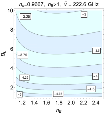
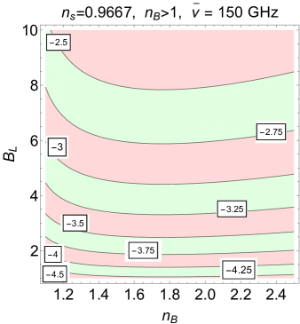
Figure 8: The angular power spectrum of the $B$-mode autocorrelation induced by the Faraday effect is illustrated for two different frequencies (i.e. $222.6$ GHz and $150$ GHz). The two plots refer to the case of blue spectra of the magnetic random field. The different labels in both plots denote the common logarithm of $\ell(\ell+1)C_{\ell}^{(\mathrm{BB})}/(2\pi)$ in units of $(\mu\mathrm{K})^{2}$ and for a $\ell=1000$ which roughly corresponds to the maximum of the $E$-mode autocorrelation entering directly the expression of Eq. (5.31). Note that, on the vertical axes, $B_{L}$ is measured in nG.

5.5 Orders of magnitudes of the $B$-mode autocorrelations

To estimate the $B$-mode autocorrelation we can use Eq. (5.31) and then evaluate the obtained result for $\ell={\mathcal{O}}(1000)$, roughly corresponding to the maximum of the $E$-mode autocorrelation. By following this strategy, the common logarithm of the $B$-mode autocorrelation induced by the Faraday effect is illustrated in Fig. 8 (in the case of blue spectral indices, i.e. $n_{\mathrm{B}}>1$) and in Fig. 9 (for red spectral indices, i.e. $n_{\mathrm{B}}<1$). In both figures the left plots correspond to a frequency channel coinciding with the maximum of the energy density of the microwave background radiation discussed in Eqs. (5.1) and (5.2). Conversely, in the right plots of Figs. 8 and 9, the frequency is instead $150$ GHz coinciding, incidentally, with the operating window of the Bicep2 experiment [101]. The various labels in the plots report the common logarithm of the $BB$ power spectrum computed from Eq. (5.31) and evaluated for $\ell=1000$.

The orders of magnitude of the $BB$ correlations of Fig. 8 can be qualitatively understood in rather simple terms. Assuming that $\overline{{\mathcal{G}}}^{(\mathrm{EE})}_{\ell}=\ell(\ell+1)C_{\ell}^{(EE)}/(2\pi)$ is well estimated by the measured angular power spectrum, we can (approximately) calculate the $E$-mode autocorrelation as:

$$\overline{{\mathcal{G}}}^{(\mathrm{EE})}_{\ell}\simeq 50\,\mu\mathrm{K}^{2},\qquad\mathrm{for}\,\,\ell\simeq\ell_{\mathrm{max}}=1000.$$ (5.37)

The actual value of the maximum of $\overline{{\mathcal{G}}}^{(\mathrm{EE})}_{\ell}$ is slightly overestimated but Eq. (5.37) is purposely generous with the aim of establishing an order of magnitude estimate valid for $\ell={\mathcal{O}}(\ell_{\mathrm{max}})$. From the analysis of Ref. [213] and from the explicit analytic expression of Eqs. (5.31) and (5.33), the order of magnitude of the $B$-mode autocorrelation is then given by:

$${\mathcal{G}}_{\ell}^{(\mathrm{BB})}\simeq 4.9\times 10^{-4}\times\biggl{(}\frac{B_{\mathrm{L}}}{\mathrm{nG}}\biggr{)}^{2}\biggl{(}\frac{150\,\mathrm{GHz}}{\overline{\nu}}\biggr{)}^{4}\,\mu\mathrm{K}^{2}\,\,\,n_{\mathrm{B}}>1.$$ (5.38)

For smaller multipoles we have that ${\mathcal{G}}^{(\mathrm{EE})}_{\ell}<5\,\mu\mathrm{K}^{2}$. This means that Eq. (5.38) should be corrected by a factor ${\mathcal{O}}(10^{-4})$; in other words for $\ell<100$ we will have that ${\mathcal{G}}_{\ell}^{(\mathrm{BB})}<10^{-5}(B_{\mathrm{L}}/\mathrm{nG})^{2}[\overline{\nu}/(150\mathrm{GHz})]^{-4}\,\,\mu\mathrm{K}^{2}$. This point can be appreciated by looking at Figs. 10, 11 and 12 where the explicit angular power spectra have been illustrated by adapting the results of Ref. [213].

The benchmark frequency of Eq. (5.38) is close to the maximum of the brightness of the CMB spectrum and it coincides, for immediate convenience, with the Bicep2 [101] operating frequency. As we saw in section 4 the value of $1$ nG for the magnetic field intensity is barely compatible with the distortions produced by a magnetic random field on the measured temperature and polarization anisotropies: this is the reason why we used the nG strength as a reference value in Eq. (5.38).

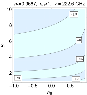
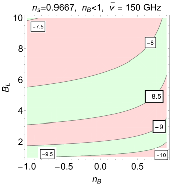
Figure 9: The angular power spectrum of the $B$-mode autocorrelation induced by the Faraday effect is illustrated for two different frequencies (i.e. $222.6$ GHz and $150$ GHz) and in the case of red spectra of the magnetic random field. As in the case of Fig. 9, the different labels in both plots denote the common logarithm of $\ell(\ell+1)C_{\ell}^{(\mathrm{BB})}/(2\pi)$ in units of $(\mu\mathrm{K})^{2}$ and for a $\ell=1000$. As in Fig. 8, $B_{L}$ is measured in nG.

When the magnetic power spectrum is red (i.e. $n_{\mathrm{B}}<1$) the values of the $B$-mode autocorrelation are ${\mathcal{O}}(10^{-4})$ smaller than in the case of blue spectra (see Fig. 9); they can be qualitatively captured by the analog of Eq. (5.38):

$${\mathcal{G}}_{\ell}^{(\mathrm{BB})}\simeq 5\times 10^{-8}\times\biggl{(}\frac{B_{\mathrm{L}}}{\mathrm{nG}}\biggr{)}^{2}\biggl{(}\frac{150\,\mathrm{GHz}}{\overline{\nu}}\biggr{)}^{4}\,\mu\mathrm{K}^{2}\,\,\,n_{\mathrm{B}}<1.$$ (5.39)

Even Eqs. (5.38) and (5.39) can only be correct within an order of magnitude, they are useful together with Figs. 8 and 9 for swift qualitative estimates. For instance the Bicep2 measurement claimed a $B$-mode detection [101] which quickly turned out to be a foreground effect. Even if confirmed, the Bicep2 measurement (i.e. ${\mathcal{G}}_{\ell}^{(\mathrm{BB})}\simeq(5.07\pm 1.13)\times 10^{-2}\,\,\mu\mathrm{K}^{2}$ for $\ell\simeq 248$) could not have been the effect of Faraday rotation [213]. This conclusion follows from a qualitative analysis of Eq. (5.38): the purported Bicep2 observation could have been only reproduced for $B_{\mathrm{L}}={\mathcal{O}}(10)$ nG which is forbidden by the analysis of the magnetized temperature and polarization anisotropies. This conclusion fits well with the results of more sophisticated discussions like the ones illustrated in Figs. 10, 11 and 12.

In Figs. 10, 11 and 12 with the full, dashed and dot-dashed lines we report the results for the $BB$ spectrum induced by the Faraday effect and numerically computed on the basis of Eq. (5.31) after having included the magnetic fields in the Einstein-Boltzmann hierarchy.

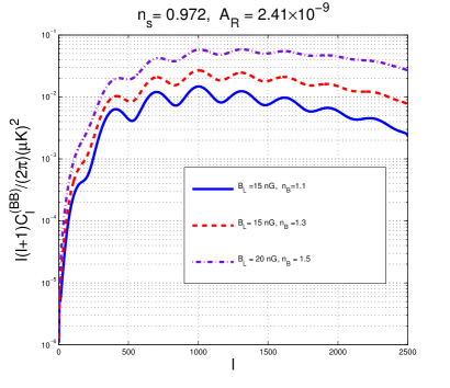
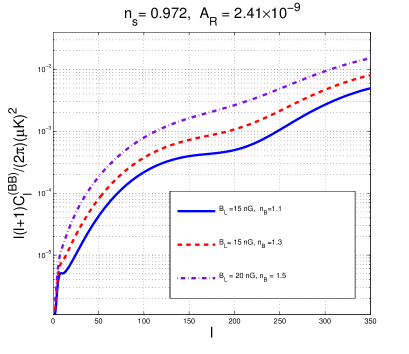
Figure 10: The $B$ mode polarization induced by the Faraday effect in the magnetized $\Lambda$CDM scenario with no tensors and with different choices of magnetic field parameters. The plot on the right illustrates the large angular scales. The axes are semilogarithmic and the frequency is $150$ GHz. The plots are adapted from Ref. [213].

Both plots of Fig. 10 share the same parameters but the plot on the right is focussed on the large angular scales while the plot on the left illustrates the small angular scales. Semilogarithmic scales are used in both plots. We can already see that the angular power spectra can only be ${\mathcal{O}}(10^{-2})\,\mu\mathrm{K}^{2}$ when $B_{\mathrm{L}}={\mathcal{O}}(15)$ nG. This trend is confirmed by Figs. 11 and 12. In Fig. 11 the magnetic spectral index has been fixed at $n_{\mathrm{B}}=1.5$ while in Fig. 12 the spectral index has been fixed to $n_{\mathrm{B}}=2$. The full, dashed and dot-dashed curves in the various plots of Figs. 11 and 12 denote, respectively magnetic field intensities of $1$, $5$ and $10$ nG.

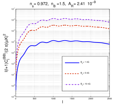
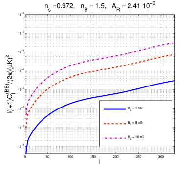
Figure 11: The $B$ mode polarization induced by the Faraday effect in the magnetized $\Lambda$CDM. In both plots the magnetic spectral index is $n_{\mathrm{B}}=1.5$. The plot on the right describes large angular scales. The axes are semilogarithmic in both plots.

We finally remind that the tensor modes of the geometry could also produce a $B$-mode polarization. The effect of the tensor modes of inflationary origin is customarily parametrized in term of the tensor to scalar ratio $r_{\mathrm{T}}$ introduced in Eq. (2.53) (see also the last line of Tab. 3 and the discussion therein). For a tensor to scalar ratio $r_{\mathrm{T}}={\mathcal{O}}(0.1)$ (which corresponds to the most recent limits) the tensor modes of inflationary origin are always larger than the one of the Faraday effect (at least for $B_{\mathrm{L}}<\mathrm{nG}$). One could however argue that even in the absence of tensor modes of inflationary origin the magnetic random fields may induce tensor modes and hence a $B$-mode. Using the same accuracy of Eq. (5.38) we can estimate that, in this case, the $BB$ power spectrum will be ${\mathcal{G}}_{\ell}^{(\mathrm{BB})}\simeq 10^{-4}(B_{\mathrm{L}}/\mathrm{nG})^{4}$. Since, however, $B_{\mathrm{L}}$ is smaller than the nG the Faraday rotation signal always dominates being proportional to $(B_{\mathrm{L}}/\mathrm{nG})^{2}$ rather than to $(B_{\mathrm{L}}/\mathrm{nG})^{4}$.

5.6 Faraday scaling

The frequency scaling induced by the Faraday effect is the most powerful tool to disambiguate the possible origin of the $B$-mode polarization. The $BB$ angular power spectrum induced by the tensor modes is frequency independent. Conversely, given the signal at a certain pivot frequency $\nu_{p}$ the B mode polarization induced by Faraday rotation at a different observational frequency $\nu$ can be obtained in terms of this simple scaling law:

$${\mathcal{G}}^{(\mathrm{BB})}_{\ell}(\overline{\nu})=\biggl{(}\frac{\overline{\nu}_{p}}{\overline{\nu}}\biggr{)}^{4}{\mathcal{G}}^{(\mathrm{BB})}_{\ell}(\overline{\nu}_{p}).$$ (5.40)

A direct application of Eq. (5.40) involves the possibility of distinguishing a potential $B$-mode signal from known unwanted foregrounds. For instance both the synchrotron and the free-free emissions lead to a frequency dependence of the $B$-mode angular power spectrum which is however very different from the one of the Faraday rotated $E$-mode polarization.

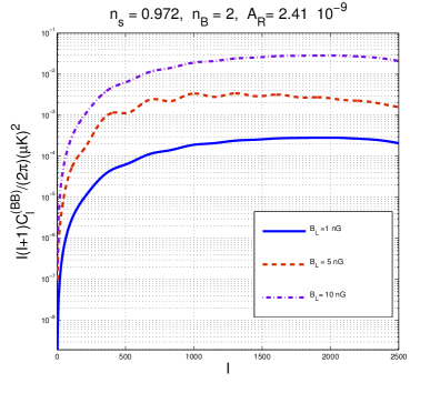
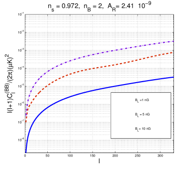
Figure 12: The $B$ mode polarization induced by the Faraday effect in the magnetized $\Lambda$CDM. In both plots the magnetic spectral index is $n_{\mathrm{B}}=2$. The plot on the right describes large angular scales. The axes are semilogarithmic in both plots.

Equation (5.40) could be used to infer the origin of the $B$-mode signal. To give an example of this second possibility let us suppose that an experiment measured ${\mathcal{G}}^{(\mathrm{BB})}_{\ell}={\mathcal{O}}(10^{-2})\,\,\mu\mathrm{K}^{2}$ at a pivot frequency $\nu_{p}=150$ GHz. Since direct upper limits on the $B$-mode autocorrelation have been presented, over different observational frequencies we could simply ask if the various upper limits are simultaneously compatible with this purported signal and with the scaling law provided by Eq. (5.40). The answer to this question is negative [216] and it has been used to exclude Faraday rotation as a possible origin of the purported Bicep2 signal [101] which was instead due to a foreground contamination.

The pivot frequencies of the microwave background polarization experiments can be conventionally divided into two ranges conventionally denoted hereunder by $\nu_{low}$ and $\nu_{high}$:

$$26\,\,\mathrm{GHz}\leq\nu_{low}\leq 36\,\,\mathrm{GHz},\qquad 100\,\,\mathrm{GHz}\leq\nu_{high}\leq 150\,\,\mathrm{GHz}.$$ (5.41)

The Dasi (Degree Angular Scale Interferometer) [80, 217] and the Cbi (Cosmic Background Imager) [218] experiments were both working in a range coinciding exactly with $\nu_{low}$. Four other experiments have been conducted around $\nu_{high}$ and they are: i) Boomerang (Balloon Observations of Millimetric Extragalactic Radiation and Geophysics) working at $145$ GHz with four pairs of polarization sensitive bolometers [219]; ii) Maxipol (Millimiter Anisotropy experiment Imaging array) working at $140$ GHz with 12 polarimeters [220]; iii) Quad working with 31 pairs of polarization sensitive bolometers: 12 at $100$ GHz and $19$ at $150$ GHz [221, 222]; iv) Bicep2 [223, 224] and its precursor Bicep1 [225] working, respectively, at $150$ GHz and $100$ GHz.

References	Data	$B_{\mathrm{L}}$	$n_{\mathrm{B}}$	Frequency
[89]	Planck	$B_{\mathrm{L}}<1.38\,\mu\mathrm{G}$	$\mathrm{undetermined}$	$70$ GHz
[102]	Polarbear	$B_{\mathrm{L}}<93$ nG	$n_{\mathrm{B}}\to 1$	$148$ GHz
[224]	Bicep2	$B_{\mathrm{L}}<30$ nG	$n_{\mathrm{B}}\to 1$	$150$ GHz
[210, 216]	Cbi	$B_{\mathrm{L}}<15$ nG	$1.1\leq n_{\mathrm{B}}<2.5$	$30$ GHz
[210, 216]	Capmap	$B_{\mathrm{L}}<10$ nG	$1.1\leq n_{\mathrm{B}}<2.5$	$35$–$46$ GHz

Table 5: The bounds inferred from direct limits on the $B$-mode polarization at low frequencies are compared with the most recent (and less restrictive) limits over larger frequencies.

There are finally four polarization sensitive experiments working in mixed or intermediate frequency ranges. They include: a) the WMAP experiment [84] (see also [226]) spanning five frequencies from $23$ to $94$ GHz; b) the Capmap experiment (Cosmic Anisotropy Polarization Mapper) [227], with $12$ receivers operating between $84$ and $100$ GHz and four receivers operating between $35$ and $46$ GHz; c) the Quiet (Q/U imager experiment) [98, 228] operating at $43$ GHz (during the first season of the experiment) and at $95$ GHz (during the second season of the experiment). Finally we have the Planck experiment [86, 88]: the three low frequency channels (i.e. $30,\,44,\,70$ GHz) belonged to the low frequency instrument (LFI); six channels (i.e. $100,\,143,\,217,\,353,\,545,\,857$ GHz) belonged to the high frequency instrument (HFI).

The $BB$ angular power spectrum induced by the Faraday effect gets larger (and even much larger) when the frequency decreases. It is therefore expected that limits obtained for frequencies between $70$ GHz and $150$ GHz may be less constraining than the limits obtained over much smaller frequencies. The observational frequencies of Planck [89], Polarbear [102] and Bicep2 [224] give bounds on the Faraday rotated $E$-mode polarization which are sometimes less constraining than some of the previous polarization experiments operating over much smaller frequencies. This theme might suggest some useful reflections which are summarized in Tab. 5. It is finally relevant to mention that the next generation of radio-telescopes (like the daring project of the Square Kilometre Array [35]) may get their frequency capability up to $25$ GHz. The overlap between radio-astronomy and microwave background will then be observationally accessible in a frequency range where the signal due to a Faraday-induced $B$-mode is maximal.

5.7 Stochastic Faraday mixing as a Markov Process

In the standard lore the polarization of the microwave background is first generated and then it is rotated by a Faraday screen. The two steps of the process, however, cannot be neatly separated. The idea explored in Ref. [229] (see also [213]) is therefore to describe the Faraday rate as a random, stationary and approximately Markovian process. In this approach the Faraday rate $X_{F}(\vec{x},\tau)$ is not a deterministic variable but rather a stochastic process which is stationary insofar as the autocorrelation function $\Gamma(\tau_{1},\tau_{2})=\langle X_{F}(\tau_{1})X_{F}(\tau_{2})\rangle$ only depends on time differences i.e. $\Gamma(\tau_{1},\tau_{2})=\Gamma(|\tau_{1}-\tau_{2}|)$. The evolution of the brightness perturbations

$$\Delta_{\pm}^{\prime}+(\epsilon^{\prime}+n^{i}\,\partial_{i})\Delta_{\pm}={\mathcal{M}}(\vec{x},\tau)\mp 2i\,X_{F}(\vec{x},\tau)\Delta_{\pm},$$ (5.42)

becomes then a stochastic differential equation. The simplest approximation is to consider $X_{F}$ as a random variable characterized by a given probability distribution; this case has been already analyzed in the framework of the synchrotron emission [230, 231, 232] and will not be specifically analyzed here.

As an example of stationary process not delta-correlated consider the case where $\Gamma(\tau_{1}-\tau_{2})=\langle X_{F}(\tau_{1})\,X_{F}(\tau_{2})\rangle$ can take only two values $\overline{x}_{F}^{2}$ and $-\overline{x}_{F}^{2}$ and let us suppose that $X_{F}(\tau)$ has switched an even number of times in the interval between $\tau_{1}$ and $\tau_{2}$ so that $\Gamma(\tau_{1}-\tau_{2})=\overline{x}_{F}^{2}$ whereas the correlation function gives $-\overline{x}_{F}^{2}$ if there have been an odd number of switches. If $p(n,\Delta\tau)$ is the probability of $n$ switches in the interval $\Delta\tau=\tau_{1}-\tau_{2}$, it follows that

$$\Gamma(\Delta\tau)=\overline{x}_{F}^{2}\sum_{n=0,\,2,\,4\,...}^{\infty}p(n,\Delta\tau)-\overline{x}_{F}^{2}\sum_{n=1,\,3,\,5\,...}^{\infty}p(n,\Delta\tau)=\overline{x}_{F}^{2}\sum_{n=0}^{\infty}(-1)^{n}\,p(n,\Delta\tau).$$ (5.43)

As the switches are random with average rate $r$, $p(n,\Delta\tau)$ is nothing but a Poisson distribution with mean number of switches $\overline{n}=r\,\Delta\tau$, i.e. $p_{n}=\overline{n}^{n}e^{-\overline{n}}/n!$. This means that $\Gamma(\Delta\tau)=\overline{x}_{F}^{2}\exp{[-2r\,\Delta\tau]}$. This is an example of dichotomic Markov process [233, 234] applied to the case of stochastic Faraday rate.

Using the technique of the cumulant expansion [233, 234] and in the absence of a primordial tensor contribution the angular power spectra of the $E$-mode and of the $B$-mode polarizations can be derived and they are:

$$C_{\ell}^{(EE)}(\omega_{F})=e^{-\omega_{F}}\,\cosh{\omega_{F}}\,\overline{C}_{\ell}^{(EE)},\qquad C_{\ell}^{(BB)}(\omega_{F})=e^{-\omega_{F}}\,\sinh{\omega_{F}}\,\overline{C}_{\ell}^{(EE)};$$ (5.44)

where

$$\omega_{F}=4\int_{\tau_{*}}^{\tau}\,d\tau_{1}\,\int_{\tau_{*}}^{\tau}\,d\tau_{2}\langle X_{F}(\tau_{1})\,X_{F}(\tau_{2})\rangle.$$ (5.45)

In Eq. (5.45) $\tau_{*}$ denotes the photon decoupling. Even if $X_{F}\leq 1$, $\omega_{F}$ is not bound to be smaller than $1$. However if $|\omega_{F}|<1$, from Eq. (5.45) $C_{\ell}^{(EE)}\simeq\overline{C}_{\ell}^{(EE)}$ while $C_{\ell}^{(BB)}\simeq\omega_{F}\overline{C}_{\ell}^{(EE)}$.

If the $B$-mode polarization induced by the tensor modes of the geometry is instead present [235], the stochastic Faraday mixing also affects the tensor modes of the geometry and the analog of the result mentioned above is given by:

$$C_{\ell}^{(EE)} = e^{-\omega_{F}}\cosh{\omega_{F}}\,\biggl{(}\overline{C}_{\ell}^{(EE)}+{\mathcal{C}}_{\ell}^{(EE)}\biggr{)}+e^{-\omega_{F}}\,\sinh{\omega_{F}}\,{\mathcal{C}}_{\ell}^{(BB)},$$

$$C_{\ell}^{(BB)} = e^{-\omega_{F}}\sinh{\omega_{F}}\biggl{(}\overline{C}_{\ell}^{(EE)}+{\mathcal{C}}_{\ell}^{(EE)}\biggr{)}+e^{-\omega_{F}}\,\cosh{\omega_{F}}\,{\mathcal{C}}_{\ell}^{(BB)};$$ (5.46)

where $\overline{C}_{\ell}^{(EE)}$ denotes the $E$ mode power spectrum coming from the scalar modes of the geometry while ${\mathcal{C}}_{\ell}^{(BB)}$ and ${\mathcal{C}}_{\ell}^{(EE)}$ (both in calligraphic style) denote, respectively, the polarization observables induced by the tensor modes of the geometry. Both the $E$ mode and the $B$ mode polarization are frequency dependent since $\omega_{F}$ is proportional to the square of the rate and, ultimately, to the fourth power of the comoving wavelength. The stochastic approach to the Faraday rate represents an ideal framework for deriving a set of scaling laws only involving the measured polarization power spectra [229, 216]. Note that Eq. (5.46) not only describes the rotation of an initial $E$-mode polarization but also the inverse effect, i.e. the rotation of an initial $B$-mode polarization of tensor origin.

6 Circular polarizations?

Large-scale magnetic fields prior to decoupling may also circular polarizations. Direct limits on the $V$-mode power spectrum between $10^{-7}\,\,\mu\mathrm{K}^{2}$ and $10^{-4}\,\,\mu\mathrm{K}^{2}$ could directly rule out (or rule in) pre-decoupling magnetic fields in the range of $0.1$–$1$ nG for typical frequencies between $10$ GHz and $30$ GHz.

6.1 The $V$-mode polarization of the microwave background

The intensity (i.e. $I=|\vec{E}\cdot\hat{e}_{1}|^{2}+|\vec{E}\cdot\hat{e}_{2}|^{2}$) and the circular polarizations (i.e. $V=2\,\mathrm{Im}[(\vec{E}\cdot\hat{e}_{1})^{*}(\vec{E}\cdot\hat{e}_{2})]$), are both invariant for a rotation of $\hat{e}_{1}$ and $\hat{e}_{2}$ in the plane orthogonal to the direction of propagation of the radiation (see also Eqs. (5.18) and (5.19)). The $V$-mode polarization is then described by two supplementary power spectra: the $V$-mode autocorrelation (i.e. the $VV$ spectrum) and the cross-correlation with the temperature (i.e. the $VT$ spectrum). The $VV$ and the $VT$ power spectra are the analog of the $EE$ and $TE$ power spectra arising in the case of the linear polarization. The $TT$, $VT$ and the $VV$ power spectra shall be preferentially considered hereunder since they are anyway larger than the $VE$ and $VB$ correlations.

In the absence of pre-decoupling magnetic field the primeval circular polarization is decoupled from the temperature fluctuations and from the linear polarization. A computable amount of circular polarization is then generated when the electron-photon scattering takes place in a magnetized environment, as previously discussed in section 2. In this case the circular polarization directly affects both the temperature anisotropies as well as the $E$-mode and $B$-mode polarizations. Thus a primordial $V$-mode polarization (possibly present prior to decoupling) can be constrained by using the magnetized plasma as a polarimeter. Conversely if the circular polarization vanishes initially the magnetic field acts effectively as a polarizer.

When the curvature perturbations are the dominant source of large-scale inhomogeneity, the evolution equations for the brightness perturbations can be derived from Eqs. (2.78), (2.79), (2.80) and (2.81). In this case, the evolution of relevant the brightness perturbations is given by:

$$\Delta_{\mathrm{I}}^{\prime}+(ik\mu+\epsilon^{\prime})\Delta_{\mathrm{I}} = \psi^{\prime}-ik\mu\phi+\epsilon^{\prime}\biggl{[}\Delta_{\mathrm{I}0}+\mu v_{\mathrm{b}}-\frac{P_{2}(\mu)}{2}S_{\mathrm{P}}\biggr{]}$$ (6.1)

$$- \frac{3}{2}i\,\epsilon^{\prime}\,f_{\mathrm{e}}(\overline{\omega})\,(1+\mu^{2})\Delta_{\mathrm{V}1}$$

$$\Delta_{\mathrm{P}}^{\prime}+(ik\mu+\epsilon^{\prime})\Delta_{\mathrm{P}} = \frac{3}{4}(1-\mu^{2})\epsilon^{\prime}S_{\mathrm{P}}-\frac{3}{2}i\epsilon^{\prime}f_{\mathrm{e}}(\overline{\omega})(\mu^{2}-1)\Delta_{\mathrm{V}1},$$ (6.2)

$$\Delta_{\mathrm{V}}^{\prime}+(ik\mu+\epsilon^{\prime})\Delta_{\mathrm{V}} = \epsilon^{\prime}\mu\biggl{\{}f_{\mathrm{e}}(\overline{\omega})[2\Delta_{\mathrm{I}0}-S_{\mathrm{P}}]-\frac{3}{2}i\Delta_{\mathrm{V}1}\biggr{\}},$$ (6.3)

where $f_{\mathrm{e}}(\overline{\omega})$ denotes, the ratio between the Larmor frequency of the electrons and the angular frequency of the observational channel (see also Eq. (2.65)). The limit $f_{\mathrm{e}}(\overline{\omega})\to 0$ corresponds to the standard situation where the plasma is not magnetized. While the tensor and the vector modes may also affect the $V$-mode polarization, their role is less relevant at least in the light of the concordance paradigm.

The analysis of the $V$-mode polarization calls for direct measurements of the circular polarizations of the CMB [236, 237]. While diverse circularly polarized foregrounds may exist [238] (see also, for instance, [239]), they are qualitatively different from the ones customarily considered in the case of linear polarizations. The bounds on circular polarizations coming from direct searches have a rather long history which can be traced back to the seminal contribution of Ref. [240] (see also [241, 242]) and of Ref. [243] (see also [244, 245]). The measurements of [243, 244, 245] were conducted for a typical wavelength of $6$ cm (corresponding to $\nu=4.9$ GHz) and used the Very Large Array radio-telescope in Socorro (New Mexico). Conversely the limits of [240, 241, 242] used a $\nu=33$ GHz radiometer (corresponding to a wavelength of $9$ mm) which used a Faraday rotator to switch between orthogonal and linear polarization states. The bounds of Ref. [240, 241, 242] and [243, 244, 245] have been used in Refs. [236, 237]. Recently further measurements appeared in the literature. Improved upper limits on the circular polarization on large angular scale have been presented in [238, 246]. Direct constraints at intermediate angular scales appeared in the literature [247] thanks to the Spider collaboration. To be relevant for the ideas conveyed in this section the present sensitivities should be improved, in the future, by at least $6$ or even $7$ orders of magnitude.

Besides the presence of a magnetic field only few other sources of circular polarization have been discussed in the literature. They include photon-photon interactions [248] and pseudo-scalar particles [207, 249]. The $V$-mode of the CMB has been also suggested as a probe for the first stars [250]. The circular polarization is finally invoked as the result of the Faraday conversion of linearly polarized radiation. Faraday conversion (typical of relativistic jets) should not be confused with Faraday rotation. In the presence of relativistic electrons linearly polarized radiation can be Faraday converted into circularly polarized radiation. The Faraday conversion and Faraday rotation have a different dependence upon the magnetic field intensity and upon the frequency [230, 231, 251]. For the latter mechanism to operate, relativistic electrons must be present in the system and this can happen only as a secondary effect when CMB photons pass through magnetized clusters; this is however not the idea pursued here since the pre-decoupling plasma is cold and the charge carriers are non-relativistic.

6.2 The magnetized plasma as a polarizer

The degree of circular polarization directly induced by the magnetized plasma can be computed from Eqs. (6.1), (6.2) and (6.3). According to this perspective the initial $V$-mode polarization vanishes so that $\Delta_{\mathrm{V}1}=0$ and the primordial circular polarization can be neglected [236, 237]. The Cauchy data for the evolution of the brightness perturbations follow, in this case, from the standard adiabatic mode (possibly even magnetized). The induced circular polarization can be computed and the results of this analysis are illustrated in Fig. 13 in the case of the standard adiabatic mode. For the fiducial set of parameters of the Planck experiment the quantitative differences are irrelevant so that we just adapted the results of Ref. [236].

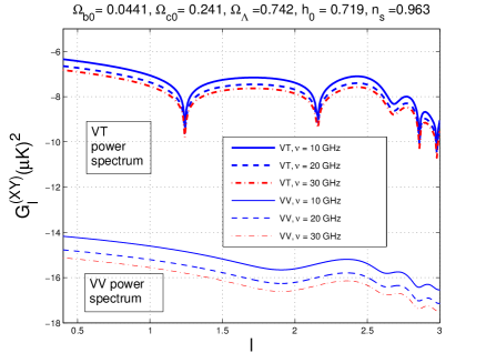
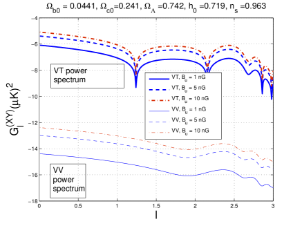
Figure 13: In the plot at the left the $VT$ and the $VV$ angular power spectra are reported for a fixed value of the magnetic field intensity $B_{u}$ (i.e. $1$ nG) but for different values of the comoving frequency. In the plot at the right the comoving frequency is fixed to $10$ GHz but the magnetic field strength increases. The thin lines denote the $VV$ correlations while the thick lines denote the $VT$ correlations. In the plots, on both axes, the common logarithm of the corresponding quantity is reported.

Note that, in Fig. 13, we denoted ${\mathcal{G}}_{\ell}^{(XY)}=\ell(\ell+1)C_{\ell}^{(XY)}/(2\pi)$ where $X=V$ and $Y$ coincides either with $V$ (in the three curves at the bottom) or with $T$ (in the three curves at the top). If the initial conditions are not adiabatic the $V$-mode polarization will have different physical features depending upon the specific entropic initial condition.

The thin lines in both plots of Fig. 13 denote the $V$-mode autocorrelations while the thick lines denote the cross-correlation of the circular polarization anisotropies with the temperature inhomogeneities. The signal is larger for low multipoles and its shape reminds a bit of the temperature autocorrelations induced by the tensor modes of the geometry which reach their largest value for small $\ell$ and decline exponentially for $\ell>90$. The $B$-mode autocorrelation induced by the tensor modes of the geometry is typically larger than the $V$-mode polarization. Recently the Spider collaboration reported a direct bound on the $V$-mode autocorrelation implying [247]

$${\mathcal{G}}_{\ell}^{(VV)}=\frac{\ell(\ell+1)C_{\ell}^{(VV)}}{2\pi}<{\mathcal{O}}(100)\mu\mathrm{K}^{2},\qquad 33<\ell<307,$$ (6.4)

for a typical frequency of $150$ GHz. The bound of [247] is actually more accurate and the term ${\mathcal{O}}(100)$ refers to constraints ranging from $141$ to $255$ $\mu\mathrm{K}^{2}$. It is also useful, in some cases, to measure the circular polarization in terms of the square root of the $VV$ angular power spectrum. Clearly if a given angular power spectrum is in the range $10^{-6}\,\mathrm{\mu}K^{2}$, its square root is of the order of $10^{-3}$ mK. These are typically the sensitivities suggested by Fig. 13.

6.3 The magnetic field as a polarimeter

If the initial radiation field is circularly polarized prior to decoupling, the problem is to deduce an upper limit on the initial degree of circular polarization. More specifically, if $\Delta_{\mathrm{V}1}\neq 0$ the line of sight solution of Eq. (6.1) implies that the power spectrum of the temperature correlations receives two separated contributions stemming, respectively, from the intensity of the radiation field (denoted by $\overline{a}^{(\mathrm{I})}_{\ell\,m}$) and from the circular polarization (denoted by $\overline{a}^{(\mathrm{V})}_{\ell\,m}$):

$$\overline{a}^{(\mathrm{I})}_{\ell\,m}=\frac{1}{(2\pi)^{3/2}}\int d^{3}k\int_{-1}^{1}\,d\mu\,\int_{0}^{2\pi}d\varphi\,Y_{\ell\,m}^{*}(\mu,\varphi)\int_{0}^{\tau_{0}}\,e^{-i\mu x}\,e^{-\epsilon(\tau,\tau_{0})}\,{\mathcal{N}}_{\mathrm{I}}(k,\mu,\tau)\,d\tau,$$ (6.5)

$$\overline{a}^{(\mathrm{V})}_{\ell\,m}=\frac{1}{(2\pi)^{3/2}}\int d^{3}k\int_{-1}^{1}\,d\mu\,\int_{0}^{2\pi}d\varphi\,Y_{\ell\,m}^{*}(\mu,\varphi)\int_{0}^{\tau_{0}}\,e^{-i\mu x}\,e^{-\epsilon(\tau,\tau_{0})}\,{\mathcal{N}}_{\mathrm{V}}(k,\mu,\tau)\,d\tau,$$ (6.6)

where the two generalized sources ${\mathcal{N}}_{\mathrm{I}}(k,\mu,\tau)$ and ${\mathcal{N}}_{\mathrm{V}}(k,\mu,\tau)$ are given, respectively, by:

$${\mathcal{N}}_{\mathrm{I}}(k,\mu,\tau)=\psi^{\prime}-ik\mu\phi+\epsilon^{\prime}\biggl{[}\Delta_{\mathrm{I}0}+\mu v_{\mathrm{b}}-\frac{1}{2}P_{2}(\mu)S_{\mathrm{P}}\biggr{]},$$ (6.7)

$${\mathcal{N}}_{\mathrm{V}}(k,\mu,\tau)=-\frac{3}{2}\,i\,\epsilon^{\prime}f_{\mathrm{e}}(\omega)(1+\mu^{2})\Delta_{\mathrm{V}1}.$$ (6.8)

The temperature fluctuation will then be the sum of the intensity contribution and of circular polarization dipole:

$$\Delta_{\mathrm{T}}(\hat{n},\tau_{0})=\sum_{\ell m}a^{(\mathrm{T})}_{\ell m}\,Y_{\ell m}(\hat{n}),\qquad a^{(\mathrm{T})}_{\ell\,m}=\overline{a}^{(\mathrm{I})}_{\ell\,m}+\overline{a}^{(\mathrm{V})}_{\ell\,m}.$$ (6.9)

It is important to appreciate that $\overline{a}^{(\mathrm{V})}_{\ell\,m}$ denotes the $V$-mode contribution to the temperature correlation and should not be confused with what we will later call $a^{(\mathrm{V})}_{\ell\,m}$ (see below Eq. (6.17)). Prior to matter-radiation equality the dipole power spectrum is given by

$${\mathcal{P}}_{\mathrm{V}}(k)={\mathcal{A}}_{\mathrm{V}}\biggl{(}\frac{k}{k_{\mathrm{p}}}\biggr{)}^{n_{\mathrm{v}}-1},\qquad k_{\mathrm{p}}=0.002\,\mathrm{Mpc}^{-1},$$ (6.10)

where, incidentally, $k_{\mathrm{p}}$ is the same pivot scale used to assign the adiabatic mode. By demanding that the $V$-mode contribution to the temperature fluctuations be negligible in comparison with the intensity, an interesting bound on the circular polarization can be derived [237]:

$${\mathcal{A}}_{V}<{\mathcal{N}}_{\mathrm{TT}}\biggl{(}\frac{{\mathcal{A}}_{{\mathcal{R}}}}{2.43\times 10^{-9}}\biggr{)}\biggl{(}\frac{z_{*}+1}{1091.79}\biggr{)}^{-2}\biggl{(}\frac{D_{A}}{14116\,\mathrm{Mpc}}\biggr{)}^{n_{v}-n_{\mathrm{s}}}\biggl{(}\frac{B_{u}}{\mathrm{nG}}\biggr{)}^{-2}\biggl{(}\frac{\nu}{\mathrm{GHz}}\biggr{)}^{2}$$ (6.11)

where $D_{A}$ denotes the (comoving) angular diameter distance to last scattering while $z_{*}$ denotes the redshift to the last scattering; the term ${\mathcal{N}}_{\mathrm{TT}}$ is given by:

$${\mathcal{N}}_{\mathrm{TT}} = 1.156\times 10^{6}\times\,(0.0354)^{n_{\mathrm{s}}-n_{v}}\,e^{-2\epsilon_{\mathrm{re}}}\,r(\ell,n_{v},n_{\mathrm{s}}),$$ (6.12)

$$r(\ell,n_{v},n_{\mathrm{s}}) = \frac{4\,\Gamma\biggl{(}\frac{3}{2}-\frac{n_{\mathrm{s}}}{2}\biggr{)}\,\Gamma\biggl{(}4-\frac{n_{v}}{2}\biggr{)}}{(n_{v}^{2}-12n_{v}+39)\Gamma\biggl{(}2-\frac{n_{\mathrm{s}}}{2}\biggr{)}\Gamma\biggl{(}\frac{3}{2}-\frac{n_{v}}{2}\biggr{)}}\,\ell^{n_{\mathrm{s}}-n_{v}}\,\biggl{[}1+{\mathcal{O}}\biggl{(}\frac{1}{\ell}\biggr{)}\biggr{]}.$$ (6.13)

where we assumed $-3<n_{v}<3$ and, moreover, $2\leq\ell<40$. The numerical value of Eq. (6.13), for different values of the spectral indices, varies btween ${\mathcal{O}}(0.1)$ (for $n_{v}>n_{\mathrm{s}}$) and ${\mathcal{O}}(10)$ (for $n_{v}<n_{\mathrm{s}}$). From Eq. (6.2), with the same logic used for the intensity, the contribution of the circular polarization to the $E$-mode autocorrelation can be computed. This analysis results is a further bound on ${\mathcal{A}}_{V}$ reading

$${\mathcal{A}}_{\mathrm{V}}<5.42\times 10^{-2}\,\sqrt{\frac{(n_{\mathrm{s}}+1)^{n_{\mathrm{s}}+1}}{(n_{v}-1)^{n_{v}-1}}}\,\biggl{(}\frac{4e}{\ell_{\mathrm{D}}}\biggr{)}^{(n_{v}-n_{\mathrm{s}})/2-1}$$

$$\times\biggl{(}\frac{{\mathcal{A}}_{{\mathcal{R}}}}{2.43\times 10^{-9}}\biggr{)}\biggl{(}\frac{z_{*}+1}{1091.79}\biggr{)}^{-2}\biggl{(}\frac{D_{A}(z_{*})}{14116\,\mathrm{Mpc}}\biggr{)}^{n_{v}-n_{\mathrm{s}}}\biggl{(}\frac{B_{u}}{\mathrm{nG}}\biggr{)}^{-2}\biggl{(}\frac{\nu}{\mathrm{GHz}}\biggr{)}^{2},$$ (6.14)

for $n_{v}>1$ and

$${\mathcal{A}}_{\mathrm{V}}<5.42\times 10^{-2}\,(2\ell_{\mathrm{V}})^{1-n_{v}}\,(n_{\mathrm{s}}+1)^{(n_{\mathrm{s}}+1)/2}\,\biggl{(}\frac{4e}{\ell_{\mathrm{D}}}\biggr{)}^{-(n_{\mathrm{s}}+1)/2}$$

$$\times\biggl{(}\frac{{\mathcal{A}}_{{\mathcal{R}}}}{2.43\times 10^{-9}}\biggr{)}\biggl{(}\frac{z_{*}+1}{1091.79}\biggr{)}^{-2}\biggl{(}\frac{D_{A}(z_{*})}{14116\,\mathrm{Mpc}}\biggr{)}^{n_{v}-n_{\mathrm{s}}}\biggl{(}\frac{B_{u}}{\mathrm{nG}}\biggr{)}^{-2}\biggl{(}\frac{\nu}{\mathrm{GHz}}\biggr{)}^{2},$$ (6.15)

for $n_{v}<1$. In Eqs. (6.14) and (refEE27) $\ell_{\mathrm{V}}={\mathcal{O}}(65)$ while $\ell_{\mathrm{D}}$ is the damping multipole appearing in the $E$-mode autocorrelations [237].

6.4 Limits on the $V$-mode autocorrelations

The contribution of the circular polarization to the $TT$ and to the $EE$ correlations can be used for the derivation of two separate sets of bounds as suggested by Eqs. (6.11) and (6.14)–(6.15). Following the discussion of Ref. [237] the following parametrization will be adopted for the direct limits on the $V$-mode power spectrum:

$$\sqrt{\frac{\ell(\ell+1)}{2\pi}C_{\ell}^{(\mathrm{VV})}}=\alpha\,T_{\gamma 0},\qquad T_{\gamma 0}=2.725\,\mathrm{K}.$$ (6.16)

Different values of $\alpha$ will correspond to different observational limits either already obtained or potentially interesting for the present considerations. Using the line of sight integration, Eq. (6.3) implies

$$a_{\ell\,m}^{(\mathrm{V})}=\frac{1}{(2\pi)^{3/2}}\int\,d\hat{n}\,Y_{\ell\,m}^{*}(\hat{n})\,\int d^{3}k\,\Delta_{\mathrm{V}}(k,\mu,\tau_{0}),$$ (6.17)

$$\Delta_{\mathrm{V}}(k,\mu,\tau_{0})=-\frac{3}{4}\,i\,\mu\int_{0}^{\tau_{0}}d\tau\,{\mathcal{K}}(\tau)\,e^{-i\mu x}\Delta_{\mathrm{V}\,1}(k,\tau).$$ (6.18)

The V-mode autocorrelation can be neatly computed in the sudden decoupling limit where the coefficient $a_{\ell\,m}^{(\mathrm{V})}$ are:

$$a_{\ell\,m}^{(\mathrm{V})}=\frac{3\,(-i)^{\ell}}{4\,(2\pi)^{3/2}}\delta_{m0}\sqrt{\frac{4\pi}{2\ell+1}}\int d^{3}k\,\int_{0}^{\tau_{0}}[\ell\,j_{\ell-1}(x)-(\ell+1)\,j_{\ell+1}(x)]\,\Delta_{\mathrm{V}\,1}(k,\tau)\,d\tau;$$ (6.19)

as usual, $x=k(\tau_{0}-\tau)$. In the large-scale limit (i.e. in practice for $\ell<40$) the angular power spectrum of the $V$-mode polarization is given by:

$$C_{\ell}^{(\mathrm{VV})}=\frac{9\pi}{4\,(2\ell+1)^{2}}\int_{0}^{\infty}\frac{dk}{k}\,{\mathcal{P}}_{V}(k)[\ell j_{\ell-1}(x)-(\ell+1)j_{\ell+1}(x)]^{2}.$$ (6.20)

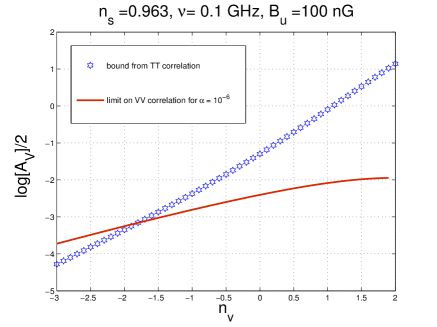
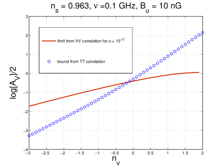
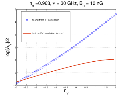
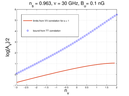
Figure 14: The bounds on the $V$-mode power spectrum are illustrated in terms of the amplitude and of the spectral index. The starred points correspond to the bounds arising from Eqs. (6.11) and (6.12). The full lines corresponds to Eq. (6.16) with the values of $\alpha$ reported in each legend.

The latter expression can be explicitly computed and the result is:

$$C_{\ell}^{(\mathrm{VV})}=\frac{9\pi^{2}}{8}{\mathcal{A}}_{\mathrm{V}}\,\biggl{(}\frac{k_{0}}{k_{\mathrm{p}}}\biggr{)}^{n_{v}-1}{\mathcal{V}}(\ell,n_{v}),$$ (6.21)

$${\mathcal{V}}(\ell,n_{v})=\frac{\ell^{2}}{(2\ell+1)^{2}}{\mathcal{V}}_{1}(\ell,n_{v})+\frac{(\ell+1)^{2}}{(2\ell+1)^{2}}{\mathcal{V}}_{2}(\ell,n_{v})-\frac{2\ell(\ell+1)}{(2\ell+1)^{2}}{\mathcal{V}}_{3}(\ell,n_{v}),$$ (6.22)

where the functions ${\mathcal{V}}_{1}(\ell,n_{v})$, ${\mathcal{V}}_{2}(\ell,n_{v})$ and ${\mathcal{V}}_{3}(\ell,n_{v})$ are given as ratios of products of Gamma functions:

$${\mathcal{V}}_{1}(\ell,n_{v}) = \frac{1}{2\sqrt{\pi}}\frac{\Gamma\biggl{(}\frac{3}{2}-\frac{n_{v}}{2}\biggr{)}\Gamma\biggl{(}\ell-\frac{3}{2}+\frac{n_{v}}{2}\biggr{)}}{\Gamma\biggl{(}2-\frac{n_{v}}{2}\biggr{)}\,\Gamma\biggl{(}\frac{3}{2}+\ell-\frac{n_{v}}{2}\biggr{)}},$$ (6.23)

$${\mathcal{V}}_{2}(\ell,n_{v}) = \frac{1}{2\sqrt{\pi}}\frac{\Gamma\biggl{(}\frac{3}{2}-\frac{n_{v}}{2}\biggr{)}\Gamma\biggl{(}\ell-\frac{1}{2}+\frac{n_{v}}{2}\biggr{)}}{\Gamma\biggl{(}2-\frac{n_{v}}{2}\biggr{)}\Gamma\biggl{(}\frac{7}{2}+\ell-\frac{n_{v}}{2}\biggr{)}},$$ (6.24)

$${\mathcal{V}}_{3}(\ell,n_{v}) = \frac{(2-n_{v})}{4\sqrt{\pi}}\frac{\Gamma\biggl{(}\frac{3}{2}-\frac{n_{v}}{2}\biggr{)}\Gamma\biggl{(}\ell-\frac{1}{2}+\frac{n_{v}}{2}\biggr{)}}{\Gamma\biggl{(}3-\frac{n_{v}}{2}\biggr{)}\Gamma\biggl{(}\frac{5}{2}+\ell-\frac{n_{v}}{2}\biggl{)}}.$$ (6.25)

As previously done, it is practical to deduce a simplified expression valid in the limit $\ell>1$:

$${\mathcal{V}}(\ell,n_{v})=\frac{\ell^{n_{v}-3}}{2\sqrt{\pi}(4-n_{v})}\frac{\Gamma\biggl{(}\frac{3-n_{v}}{2}\biggr{)}}{\Gamma\biggl{(}\frac{4-n_{v}}{2}\biggr{)}}\biggl{[}1+{\mathcal{O}}\biggl{(}\frac{1}{\ell}\biggr{)}\biggr{]}.$$ (6.26)

Since ${\mathcal{A}}_{\mathrm{V}}$ has been independently bounded from the analysis of the $TT$ and of the $EE$ angular power spectra, the $V$-mode angular power spectrum is also bounded. In Fig. 14 the bounds stemming from the $V$-mode contribution to the $TT$ power spectrum are summarized for different values of the magnetic field intensity. In all four plots on the vertical axis we report the common logarithm of $\sqrt{{\mathcal{A}}_{\mathrm{V}}}$ while on the horizontal axis the corresponding spectral index is illustrated.

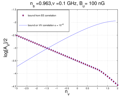
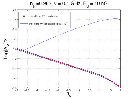
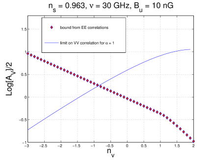
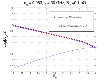
Figure 15: The bounds on the V-mode power spectrum are illustrated as they arise from the $EE$ correlations. The bounds derived in section 4 are illustrated and compared with the potentially direct bounds parametrized, as in Fig. 14, in terms of different values of $\alpha$ (see Eq. (6.16).

In Fig. 14 with the full line we report the limit on $\sqrt{{\mathcal{A}}_{\mathrm{V}}}$ stemming from Eq. (6.16) in terms of the corresponding value of $\alpha$. The various curves are obtained by using, at the left hand side of Eq. (6.16) the expression of Eq. (6.22) appropriately averaged over the multipole range. Always in Fig. 5 the starred points correspond to the bound on $\sqrt{{\mathcal{A}}_{\mathrm{V}}}$ derived in Eqs. (6.11) and (6.12).

The results of Fig. 14 suggest that for sufficiently large frequencies and for sufficiently small magnetic field intensity the bounds derived from the $TT$ correlations are not competitive with potential direct limits. This aspect can be appreciated from the two bottom plots of Fig. 5 where already a value $\alpha=1$ would imply a more stringent limit on $\sqrt{{\mathcal{A}}_{\mathrm{V}}}$. Notice that the allowed region is below the full line (if the limit of Eq. (6.16) is considered) or below the starred points if the limit of Eqs. (6.11) and (6.12) is enforced.

In connection with Figs. 14 and 15 there are three possible situations. The full line could always be above the starred line: this never happens in the case of Fig. 14 but it would simply mean that any indirect limit is more stringent than the direct one. If the full line is below the starred line the indirect limit from the $TT$ correlation is always compatible with the direct searches: this always happens if the magnetic field is sufficiently small (see, e.g. Fig. 14 bottom left plot). Finally the full line may cross the starred points: this is the most realistic situation in the light of the present and forthcoming direct limits on circular dichroism.

By looking at Fig. 14 it is plausible that, depending upon the frequency of the experiment, magnetic fields $B_{\mathrm{u}}={\mathcal{O}}(100\,\mathrm{nG})$ can be directly excluded for $\nu\simeq\mathrm{GHz}$ and with a sensitivity $\alpha\simeq 10^{-6}$ which would imply, in terms of Eq. (6.16), direct upper limits on the V-mode power spectrum ${\mathcal{O}}(\mu K)$ for $\ell<40$.

In Fig. 15 the same absolute bounds illustrated in Fig. 14 are now compared with the bounds from the analysis of the $EE$ correlations which are numerically more significant, especially for large spectral indices (i.e. $n_{v}>1$). As in the case of Fig. 14 sufficiently small values of the magnetic field intensity make the indirect bounds rather loose in comparison with direct limits. There are however numerical differences. From the top right and bottom left plots of Fig. 15 magnetic fields $B_{\mathrm{u}}={\mathcal{O}}(10\,\mathrm{nG})$ can be directly excluded for $\nu\simeq\mathrm{GHz}$ and with a sensitivity $\alpha\simeq 10^{-6}$. The bounds stemming from the $EE$ correlations are therefore more stringent than the ones derived in the case of the $TT$ correlations.

It is finally appropriate to mention that the frequency range assumed in the present discussion is in the GHz range because previous bounds, even if loose, were set over those frequencies. It is however tempting to speculate that, in a far future, microwave background measurements could be possible even below the GHz. In this case direct bounds will certainly be more stringent but huge foregrounds might make this speculation forlorn (see, in this connection, [252, 253]).

All in all, if a $V$-mode polarization (not correlated with the adiabatic mode) is present prior to matter-radiation equality both the $TT$ and the $EE$ power spectra are affected in a computable manner. Specific constraints can then be inferred in terms of the amplitude and of the spectral index of the $V$-mode power spectrum. Improved direct experimental limits on the $VV$ correlations could be used for setting a limit on the magnetic field intensity. For experimental devices operating in the GHz range, direct limits on the circular dichroism imply constraints on pre-decoupling magnetic fields in the $10$ nG range. Conversely, the current limits on large-scale magnetic fields derived from the distortions of the $TT$, $TE$ and $EE$ correlations (in the nG range) are compatible with current bounds on the primordial dichroism. Improved bounds on the $V$-mode polarization are not only interesting in their own right but they might have rewarding phenomenological implications. Direct limits on the $V$-mode power spectrum in the range ${\mathcal{O}}(0.01\,\mathrm{mK})$ imply limits on ${\mathcal{A}}_{\mathrm{V}}$ ranging from ${\mathcal{O}}(10^{-8})$ to ${\mathcal{O}}(10^{-4})$ depending on the value of the spectral index and for angular scales larger than ${\mathcal{O}}(1\,\mathrm{deg})$.

7 An ongoing trialogue

As argued more than fifty years ago by Hoyle and Zeldovich, if the origin of large-scale magnetism is primordial (as opposed to astrophysical), magnetic random fields evolving in the primeval plasma prior to the decoupling of radiation from matter must necessarily affect the microwave background observables. During the past decade the magnetized temperature and polarization anisotropies have been analyzed in the context of a serendipitous trialogue involving plasma physics, general relativity and astrophysics. This ongoing effort led to a number of interesting progresses so that today the problem is correctly formulated, at least in principle if not always in practice. Interesting constraints on magnetic random fields in the nG range have been established. The five WMAP releases and the Planck results provided a steady quantitive refinement of existing bounds (sometimes obtained with comparatively primitive methods). While the overall consistency of different approaches is rewarding from the theoretical viewpoint, it is fair to say that the primordial nature of large-scale magnetic fields has been neither confirmed nor ruled out.

Various reference sets of Cauchy data of the Einstein-Boltzmann hierarchy are customarily arranged to scrutinize the microwave background observables in the context of the concordance paradigm and of its immediate extensions. The very same strategy is a fortiori mandatory when the magnetic random fields are dynamical. Even if not all the aspects of this rich theoretical framework have been fully explored, the guiding logic developed in the past decade is that magnetic random fields cannot be generically excluded or discovered by only refining the tools of the data analyses: it is essential to understand what to look for in the data and what kind of initial conditions are more or less physical. Alternatively one should envisage specific tests that are independent on the initial data: this complementary tactic proved to be more difficult so far.

There are at least three general problems to be addressed in the near future if our course of action is to prove sound and effective. At the moment the magnetized initial conditions of the Einstein-Boltzmann hierarchy have been more or less classified but it is unclear which ones are more physical. While the adoption of the conventional adiabatic paradigm found a strong justification in the relative position of the first acoustic peak and of the first anticorrelation peak of the cross-correlation between temperature and polarization, an analog model-independent test is not yet available in the case of magnetized perturbations. Similarly, while in the conventional case there are now good reasons to eliminate the entropic initial conditions from the Cauchy data of the Einstein-Boltzmann hierarchy, we do not have any specific rationale to exclude possible compensations effects coming from the interference of entropic modes and magnetized initial conditions.

Assuming a better understanding of the Cauchy data the second interesting area of investigation involves an improved theoretical scrutiny of the Faraday effect which is certainly one of the best model-independent tests for the primordial nature of large-scale magnetism. It could be that a $B$-mode polarization of tensor origin will be soon discovered and we shall therefore be in the situation of considering the interplay of magnetic and non-magnetic sources of $B$-mode polarization. These analyses seem particularly urgent in the light of the forthcoming full-sky surveys of Faraday rotations which could even reach frequencies of $25$ GHz.

It would be highly desirable to see a steady observational progress in the analysis of circular polarizations of the microwave background. Further scrutiny of these aspects is important in its own right since the direct analyses of circular polarizations are at the moment the most challenging in the remarkable agenda of the observational cosmologists. The study of circular dichroism is not more forlorn than other signals which are often invoked as conceptually important to consider but observationally difficult to assess. While the systematic effects plaguing the measurements of the $V$-mode power spectra differ from the case of linear polarizations, whether or not they are less severe depends also upon the features of the instrument and on the specific frequency band.

It is finally plausible to expect that during the forthcoming score year a new channel for the observations of magnetic random fields will become hopefully available. Magnetic random fields may lead to a stochastic backgrounds of relic gravitational waves in the frequency interval ranging between few $\mu$Hz and $10$ kHz. This intermediate range encompasses the operating windows of space-borne interferometers (hopefully available twenty years from now) and of terrestrial detectors (already available but still insensitive to stochastic backgrounds of relic gravitons of cosmological origin). Hypermagnetic fields possibly present before and after the electroweak phase transition typically lead to a stochastic background which may even be $8$ orders of magnitude larger than the conventional inflationary contribution characterized by a spectral energy density in critical units ${\mathcal{O}}(10^{-17})$.

Given the encouraging progresses of the past decade it is fair to expect that the forthcoming years will be an exciting moment both for theory and for observations. This will be even more true if the forthcoming flow of data will not only be regarded as a source of improved precision but also as a concrete inspiration for the scrutiny of novel and potentially unexpected paradigms.

Aknowledgements

It is a pleasure to thank G. Sironi for sharing his wise remarks all along the last decade. The kind support and the encouragement of D. Pedrini is also acknowledged. Last but not least I wish to thank J. Vigen, T. Basaglia, A. Gentil-Beccot and S. Rohr of the CERN Scientific Information Service for their help and for their everlasting patience.

Appendix A Isotropic random fields

A.1 Scalar, vector and tensor random fields

For coincident (conformal) times the two-point functions of isotropic scalar, vector and tensor random fields in real space only depend on the distance $r=|\vec{x}-\vec{y}|$ between the two spatially separated points:

$${\mathcal{C}}^{(s)}(r,\tau)=\langle{\mathcal{R}}(\vec{x},\tau){\mathcal{R}}(\vec{y},\tau)\rangle,$$ (A.1)

$${\mathcal{C}}^{(v)}_{ij}(r,\tau)=\langle B_{i}(\vec{x},\tau)B_{j}(\vec{y},\tau)\rangle,$$ (A.2)

$${\mathcal{C}}^{(t)}_{ijmn}(r,\tau)=\langle h_{ij}(\vec{x},\tau)h_{mn}(\vec{y},\tau)\rangle.$$ (A.3)

In Eq. (A.1) ${\mathcal{R}}(\vec{x},\tau)$ denotes a generic scalar which can coincide, for instance, with the curvature perturbations on comoving orthogonal hypersurfaces introduced in Eqs. (2.44), (2.46) or (3.53). Similarly, in Eq. (A.2) $B_{i}(\vec{x},\tau)$ is valid for a three-dimensional vector but it also applies to the comoving electric and magnetic fields introduced in Eqs.(2.20) and (2.21). Finally, in Eq. (A.3) $h_{ij}(\vec{x},\tau)$ is a rank-two tensor in three-dimensional Euclidean space and it describes, for example, the tensor modes of the geometry or the anisotropic stress. According to the present conventions the Fourier transform of ${\mathcal{R}}(\vec{x},\tau)$ is defined as:

$${\mathcal{R}}(\vec{x},\tau)=\frac{1}{(2\pi)^{3/2}}\int d^{3}k{\mathcal{R}}(\vec{k},\tau)e^{-i\vec{k}\cdot\vec{x}}.$$ (A.4)

The power spectrum $P_{{\mathcal{R}}}(k)$ is simply given by

$$\langle{\mathcal{R}}(\vec{x},\tau)\,{\mathcal{R}}(\vec{x}+\vec{r},\tau)\rangle=\int d\ln{k}\,P_{{\mathcal{R}}}(k,\tau)\,j_{0}(kr),\qquad j_{0}(kr)=\frac{\sin{kr}}{kr},$$ (A.5)

where $j_{0}(kr)$ is the spherical Bessel function of zeroth-order [159, 160]. In Fourier space the two-point function of Eq. (A.5) is

$$\langle{\mathcal{R}}(\vec{k},\tau)\,{\mathcal{R}}(\vec{p},\tau)\rangle=\frac{2\pi^{2}}{k^{3}}P_{{\mathcal{R}}}(k,\tau)\delta^{(3)}(\vec{k}+\vec{p}).$$ (A.6)

The power spectrum of Eq. (A.6) describes the large-scale inhomogeneities of the concordance paradigm and its explicit form has been introduced in Eq. (2.52). Equations (A.5) and (A.6) power spectrum $P_{{\mathcal{R}}}(k,\tau)$ (in Fourier space) has the same dimensions of the correlation function (in real space).

The explicit expression of the two-point function of vector random fields given in Eq. (A.2) depends on three functions $M_{T}(r,\tau)$, $M_{L}(r,\tau)$ and $M_{G}(r,\tau)$ denoting, respectively, the transverse, the longitudinal and the gyrotropic components:

$${\mathcal{C}}^{(v)}_{ij}(r,\tau)=M_{T}(r,\tau)p_{ij}(\hat{r})+M_{L}(r,\tau)\hat{r}_{i}\hat{r}_{j}+M_{G}(r,\tau)\epsilon_{ij\ell}\hat{r}^{\ell},$$ (A.7)

where $p_{ij}(\hat{r})=\delta_{ij}-\hat{r}_{i}\hat{r}_{j}$ is the transverse the projector and $\hat{r}^{i}=r^{i}/r$ is the unit vector. The gyrotropic contribution, proportional to the Levi-Civita totally antisymmetric symbol, is rotationally-invariant but not parity-invariant; if present it implies the existence of a non-vanishing magnetic gyrotropy defined as $\vec{B}\cdot\vec{\nabla}\times\vec{B}$. Whenever the vector random fields are divergenceless, their transverse and the longitudinal components will be subjected to the following further condition:

$$\frac{\partial M_{L}}{\partial r}+\frac{2}{r}(M_{L}-M_{T})=0,$$ (A.8)

which follows by simply imposing that ${\mathcal{C}}^{(v)}_{ij}(r,\tau)$ be divergenceless. It could also happen that the two-point function be traceless (i.e. $2M_{T}+M_{L}=0$) but this is not what happens in the case of the magnetic random fields. In complete analogy with the scalar case of Eq. (A.4) the Fourier transform of $B_{i}(\vec{x},\tau)$ is:

$$B_{i}(\vec{x},\tau)=\frac{1}{(2\pi)^{3/2}}\int d^{3}k\,B_{i}(\vec{k},\tau)\,e^{-i\vec{k}\cdot\vec{x}}.$$ (A.9)

It follows from Eq. (A.9) that the vector power spectra are given by:

$$\langle B_{i}(\vec{k},\tau)\,B_{j}(\vec{p},\tau)\rangle=\frac{2\pi^{2}}{k^{3}}\biggl{[}P_{B}(k,\tau)\,p_{ij}(\hat{k})+{\mathcal{P}}_{G}(k,\tau)\epsilon_{ij\ell}\hat{k}^{\ell}\biggr{]}\delta^{(3)}(\vec{k}+\vec{p}).$$ (A.10)

If $B_{i}(\vec{x},\tau)$ coincides with the magnetic field its dimensions will be of an inverse area (i.e. $L^{-2}$) while $B_{i}(\vec{k},\tau)$ will obviously have dimensions of a length (i.e. $L$). This elementary remark shows in explicit terms that the magnetic power spectrum in Fourier space (i.e. Eq. (A.10)) has the same dimensions of the two point function in coordinate space (i.e. Eq. (A.2)). Since the two-point function of magnetic random fields has the dimensions of an energy density in real space, the corresponding power spectrum will be measured in the same units (e.g. $\mathrm{Gauss}^{2}$ or $\mathrm{Tesla}^{2}$). In the case of the magnetic field, $M_{T}(r,\tau)$, $M_{L}(r,\tau)$ and $M_{G}(r,\tau)$ will be given by:

$$M_{T}(r,\tau) = \int d\ln{k}\,P_{B}(k,\tau)\,\biggl{[}\frac{\cos{kr}}{k^{2}r^{2}}+\frac{k^{2}r^{2}-1}{k^{3}r^{3}}\sin{kr}\biggr{]},$$ (A.11)

$$M_{L}(r,\tau) = 2\int d\ln{k}\,P_{B}(k,\tau)\,\frac{[\sin{kr}-kr\cos{kr}]}{k^{3}r^{3}},$$ (A.12)

$$M_{G}(r,\tau) = \int d\ln{k}\,P_{G}(k,\tau)\,\biggl{[}\frac{\cos{kr}}{kr}-\frac{\sin{kr}}{k^{2}r^{2}}\biggr{]}.$$ (A.13)

Note finally that the two vector polarizations $\hat{e}_{i}^{\alpha}(\hat{k})$ (with $\alpha=1,\,2$) of the divergenceless and traceless random vector fields obey $\sum_{\alpha=1,\,2}\hat{e}^{(\alpha)}_{i}(\hat{k})\hat{e}^{(\alpha)}_{j}(\hat{k})=p_{ij}(\hat{k})$.

The explicit form of the two-point function for tensor random fields given in Eq. (A.3) can be more explicitly written as:

$${\mathcal{C}}^{(t)}_{ijmn}(r,\tau) = N_{T}(r,\tau)[p_{im}(\hat{r})p_{jn}(\hat{r})+p_{in}(\hat{r})p_{jm}(\hat{r})-p_{ij}(\hat{r})p_{mn}(\hat{r})]$$ (A.14)

$$+ N_{L}(r,\tau)\hat{r}_{i}\,\hat{r}_{j}\,\hat{r}_{m}\,\hat{r}_{n}$$

$$+ N_{G}(r,\tau)[\epsilon_{ijk}\epsilon_{mn\ell}\,\hat{r}^{k}\,\hat{r}^{\ell}+\epsilon_{imk}\epsilon_{jn\ell}\,\hat{r}^{k}\,\hat{r}^{\ell}+\epsilon_{ink}\,\epsilon_{jm\ell}\,\hat{r}^{k}\,\hat{r}^{\ell}].$$

Following the same conventions of Eqs. (A.4) and (A.9) the Fourier transform of $h_{ij}(\vec{x},\tau)$ is defined as

$$h_{ij}(\vec{x},\tau)=\frac{1}{(2\pi)^{3/2}}\int d^{3}k\,h_{ij}(\vec{k},\tau)\,e^{-i\vec{k}\cdot\vec{x}}.$$ (A.15)

Neglecting the terms that break explicitly parity and that are antisymmetric in $(ij)$ or $(mn)$, the two-point function traced over the indices and the correlation function in Fourier space are, respectively,

$$\langle h_{ij}(\vec{x},\tau)h_{ij}(\vec{x}+\vec{r},\tau)\rangle = \int d\ln{k}\,P_{\mathrm{T}}(k,\tau)j_{0}(kr),$$ (A.16)

$$\langle h_{ij}(\vec{k},\tau)\,h_{mn}(\vec{p},\tau)\rangle = \frac{2\pi^{2}}{k^{3}}P_{\mathrm{T}}(k,\tau)\,{\mathcal{S}}_{ijmn}(\hat{k})\,\delta^{(3)}(\vec{k}+\vec{p}),$$ (A.17)

$${\mathcal{S}}_{ijmn}(\hat{k}) = \frac{1}{4}\biggl{[}p_{im}(\hat{k})p_{jn}(\hat{k})+p_{in}(\hat{k})p_{jm}(\hat{k})-p_{ij}(\hat{k})p_{mn}(\hat{k})\biggr{]},$$ (A.18)

where ${\mathcal{S}}_{ijmn}(\hat{k})$ is traceless and divergenceless as implied by the requirement $h_{i}^{i}=\partial_{i}h^{ij}=0$:

$$\hat{k}^{i}{\mathcal{S}}_{ijmn} = \hat{k}^{j}{\mathcal{S}}_{ijmn}=\hat{k}^{m}{\mathcal{S}}_{ijmn}=\hat{k}^{n}{\mathcal{S}}_{ijmn}=0,$$ (A.19)

$${\mathcal{S}}_{iimn}(\hat{k}) = {\mathcal{S}}_{ijmm}(\hat{k})=0,\qquad{\mathcal{S}}_{ijij}(\hat{k})=1.$$ (A.20)

The two tensor polarizations are defined in this paper as

$$\hat{e}^{\oplus}_{ij}(\hat{k})=\hat{m}_{i}\hat{m}_{j}-\hat{n}_{i}\hat{n}_{j},\qquad\hat{e}^{\otimes}_{ij}(\hat{k})=\hat{m}_{i}\hat{n}_{j}+\hat{n}_{i}\hat{m}_{j},$$ (A.21)

where $\hat{m}$, $\hat{n}$ and $\hat{k}$ are a triplet of mutually orthogonal unit vectors. The sum over the polarizations leads, respectively, to

$$\sum_{\beta=\oplus,\,\otimes}\hat{e}^{(\beta)}_{ij}(\hat{k})\hat{e}^{(\beta)}_{mn}(\hat{k})=p_{im}(\hat{k})p_{jn}(\hat{k})+p_{in}(\hat{k})p_{jm}(\hat{k})-p_{ij}(\hat{k})p_{mn}(\hat{k})=4{\mathcal{S}}_{ijmn}(\hat{k}).$$ (A.22)

A.2 Vector identities and further power spectra

The explicit components of the canonical energy-momentum tensor of Eq. (2.12) are:

$$T_{0}^{(EM)\,0} = \delta_{\mathrm{s}}\rho_{\mathrm{E}}(\vec{x},\tau)+\delta_{\mathrm{s}}\rho_{\mathrm{B}}(\vec{x},\tau),$$ (A.23)

$$T_{i}^{(EM)\,j} = -\biggl{[}\delta_{\mathrm{s}}p_{\mathrm{E}}(\vec{x},\tau)+\delta_{\mathrm{s}}p_{\mathrm{B}}(\vec{x},\tau)\biggr{]}\delta_{i}^{j}+\Pi^{(\mathrm{E})\,j}_{i}(\vec{x},\tau)+\Pi^{(\mathrm{B})\,j}_{i}(\vec{x},\tau),$$ (A.24)

$$T_{0}^{(EM)\,i} = \frac{1}{4\pi a^{4}}\biggl{(}\vec{E}\times\vec{B}\biggr{)}^{i},$$ (A.25)

where $\vec{E}$ and $\vec{B}$ are the comoving electric and magnetic fields introduced in Eqs. (2.19), (2.20) and (2.21). The energy densities already introduced in Eq. (3.39) are preceded by $\delta_{\mathrm{s}}$ since they only affect the evolution of the scalar modes of the geometry. Conversely the magnetic and the electric anisotropic stresses $\Pi^{(\mathrm{B})}_{ij}$ and $\Pi^{(\mathrm{E})}_{ij}$ (already defined in Eq. (3.46)) not only contribute to the evolution of the scalar modes but also to the vector and tensor fluctuations of the geometry. In the case of the electric fields the following vector identity can be easily derived:

$$\frac{\vec{\nabla}\cdot[(\vec{\nabla}\times\vec{E})\times\vec{E}]}{4\pi a^{4}(\rho_{\gamma}+p_{\gamma})}=\nabla^{2}\biggl{[}\sigma_{E}-\frac{\Omega_{E}}{4}\biggr{]}-\frac{3}{16\pi\rho_{\gamma}a^{4}}(\vec{\nabla}\cdot\vec{E})^{2}$$ (A.26)

where, $\Omega_{\mathrm{E}}$ and $\sigma_{\mathrm{E}}$ have been introduced, respectively, in Eqs. (3.40) and (3.49). A similar vector identity holds in the case of the magnetic field in the approximation where the total current is solenoidal namely

$$\frac{3}{4}\frac{\vec{\nabla}\cdot[\vec{J}\times\vec{B}]}{a^{4}\rho_{\gamma}}=\nabla^{2}\sigma_{\mathrm{B}}-\frac{1}{4}\nabla^{2}\Omega_{\mathrm{B}},$$ (A.27)

where, as in Eqs. (3.40) and (3.49), we have referred the magnetic energy density and the corresponding anisotropic stress to the photon background. After simple algebra Eq. (A.27) can also be written as:

$$\nabla^{2}\sigma_{\mathrm{B}}=\frac{3}{16\pi\rho_{\gamma}a^{4}}\partial_{i}B_{j}\partial^{j}B^{i}-\frac{1}{2}\nabla^{2}\Omega_{\mathrm{B}}.$$ (A.28)

If the plasma is globally neutral also the electric field is solenoidal so that Eqs. (A.26) and (A.27) are symmetric. In the slow description of the plasma modes summarized in Eq. (3.24) the total current, the magnetic fields and the electric field are all solenoidal.

Since $\Omega_{\mathrm{B}}(\vec{x},\tau)$ and $\sigma_{\mathrm{B}}(\vec{x},\tau)$ are scalars we can compute their associated power spectra. Recalling the conventions of Eqs. (A.4) and (A.6) in Fourier space their expression is:

$$\Omega_{\mathrm{B}}(\vec{q},\tau) = \frac{1}{(2\pi)^{3/2}}\frac{1}{8\pi a^{4}\rho_{\gamma}}\int d^{3}kB_{i}(k,\tau)B^{i}(\vec{q}-\vec{k},\tau),$$ (A.29)

$$\sigma_{\mathrm{B}}(\vec{q},\tau) = \frac{1}{(2\pi)^{3/2}}\frac{1}{16\pi a^{4}\rho_{\gamma}}\int d^{3}k\biggl{[}\frac{3(q^{j}-k^{j})k^{i}}{q^{2}}B_{j}(k,\tau)B_{i}(\vec{q}-\vec{k},\tau)$$ (A.30)

$$- B_{i}(\vec{q}-\vec{k},\tau)B^{i}(\vec{k},\tau)\biggr{]}.$$

The correlation functions for $\Omega_{\mathrm{B}}(\vec{k},\tau)$ and $\sigma_{\mathrm{B}}(\vec{k},\tau)$ are then defined as

$$\langle\Omega_{\mathrm{B}}(\vec{q},\tau)\Omega_{\mathrm{B}}(\vec{p},\tau)\rangle = \frac{2\pi^{2}}{q^{3}}P_{\Omega}(q,\tau)\delta^{(3)}(\vec{q}+\vec{p}),$$

$$\langle\sigma_{\mathrm{B}}(\vec{q},\tau)\sigma_{\mathrm{B}}(\vec{p},\tau)\rangle = \frac{2\pi^{2}}{q^{3}}P_{\sigma}(q,\tau)\delta^{(3)}(\vec{q}+\vec{p}).$$ (A.31)

Defining, for the sake of simplicity, the following auxiliary scalar product

$$\gamma(\vec{k},\vec{q})=\frac{\vec{k}\cdot(\vec{q}-\vec{k})}{k|\vec{q}-\vec{k}|}=\frac{\hat{k}\cdot(\vec{q}-\vec{k})}{|\vec{q}-\vec{k}|},$$ (A.32)

the explicit expression of the two power spectra $P_{\Omega}(q,\tau)$ and $P_{\sigma}(q,\tau)$ is given in terms of the power spectra of the magnetic random fields as:

$$P_{\Omega}(q,\tau) = \frac{q^{3}}{(2\pi)}\frac{1}{8\pi a^{4}\rho_{\gamma}}\int d^{3}k\frac{P_{\mathrm{B}}(k,\tau)}{k^{3}}\frac{P_{\mathrm{B}}(|\vec{q}-\vec{k}|,\tau)}{|\vec{q}-\vec{k}|^{3}}\biggl{[}1+\gamma^{2}(\vec{k},\vec{q})\biggr{]},$$ (A.33)

$$P_{\sigma}(q,\tau) = \frac{q^{3}}{(2\pi)}\frac{1}{(16\pi a^{4}\rho_{\gamma})^{2}}\int d^{3}k\frac{P_{\mathrm{B}}(k,\tau)}{k^{3}}\frac{P_{\mathrm{B}}(|\vec{q}-\vec{k}|,\tau)}{|\vec{q}-\vec{k}|^{3}}$$ (A.34)

$$\times \biggl{\{}1+\gamma^{2}(\vec{k},\vec{q})+\frac{6\,\vec{k}\cdot(\vec{q}-\vec{k})}{q^{2}}\biggl{[}1-\gamma^{2}(\vec{k},\vec{q})\biggr{]}$$

$$+ \frac{9\,k^{2}|\vec{q}-\vec{k}|^{2}}{q^{4}}\biggl{[}1-\gamma^{2}(\vec{k},\vec{q})\biggr{]}^{2}\biggr{\}}.$$

The source terms for the evolution of the scalar modes of the geometry are visibly the most cumbersome since they involve the energy density, the pressure and the anisotropic stress. For the vector and for the tensor modes the source terms only involve the vector and the tensor components of the electromagnetic anisotropic stress. For instance, in the case of the magnetic fields we can always write:

$$\Pi_{ij}^{(\mathrm{B})}(\vec{q},\tau) = \Pi_{ij}^{(scal,\mathrm{B})}(\vec{q},\tau)+\Pi_{ij}^{(vec,\mathrm{B})}(\vec{q},\tau)+\Pi_{ij}^{(ten,\mathrm{B})}(\vec{q},\tau),$$ (A.35)

$$\Pi_{ij}^{(scal,\mathrm{B})}(\vec{q},\tau) = \hat{q}_{i}\hat{q}_{j}\Pi_{ij}^{(\mathrm{B})}(\vec{q},\tau),$$ (A.36)

$$\Pi_{ij}^{(vec,\mathrm{B})}(\vec{q},\tau) = \biggl{[}p_{in}(\hat{q})\,\hat{q}_{j}+p_{jn}(\hat{q})\,\hat{q}_{i}\biggr{]}\hat{q}_{m}\Pi_{mn}^{(\mathrm{B})}(\vec{q},\tau),$$ (A.37)

$$\Pi_{ij}^{(tens,\mathrm{B})}(\vec{q},\tau) = \biggl{[}p_{im}(\hat{q})\,p_{jn}(\hat{q})+p_{jn}(\hat{q})\,p_{im}(\hat{q})\biggr{]}\Pi_{mn}^{(\mathrm{B})}(\vec{q},\tau),$$ (A.38)

where, by definition, the Fourier transform of the total magnetic anisotropic stress is given by:

$$\Pi_{mn}^{(\mathrm{B})}(\vec{q},\tau)=\frac{1}{4\pi a^{4}\,(2\pi)^{3/2}}\int d^{3}k\biggl{[}B_{m}(\vec{k},\tau)B_{n}(\vec{q}-\vec{k},\tau)-\frac{1}{3}B_{\ell}(\vec{k},\tau)B_{\ell}(\vec{q}-\vec{k},\tau)\delta_{mn}\biggr{]}.$$ (A.39)

Equations (A.29)–(A.30) as well as Eqs. (A.31), (A.33) and (A.34) can be rephrased in terms of the electric random fields at least as long as they are solenoidal, exactly as the magnetic random fields or the total current.

A.3 Parameters of the magnetized $\Lambda$CDM scenario

Even if, according to Eq. (4.2), the initial conditions of the Einstein-Boltzmann could be assigned directly in terms of the amplitude $A_{\mathrm{B}}$ and of the spectral index, it is a common practice to trade $A_{\mathrm{B}}$ for the regularized magnetic energy density $B_{\mathrm{L}}^{2}$. When the magnetic power spectra are blue (i.e. $n_{\mathrm{B}}>1$) the energy density is predominantly concentrated over small scales; the opposite is true for the case of red spectra (i.e. $n_{\mathrm{B}}<1$). From Eqs. (A.7) and (A.10), $B_{\mathrm{L}}^{2}$ is the trace of the two-point function of the magnetic random fields:

$$B_{\mathrm{L}}^{2}={\mathcal{C}}^{(v)}_{ii}(r,\tau)=\langle B_{i}(\vec{x},\tau)B^{i}(\vec{y},\tau)\rangle=2\int d\ln{k}P_{\mathrm{B}}(k,\tau)j_{0}(kr)W(k),$$ (A.40)

where $W(k)$ is an appropriate window function which is not strictly necessary and could be simply replaced either by an ultraviolet cut-off (in the case of blue spectra) or by an infra-red cut-off (in the case of red spectra).

When the spectrum is blue the energy density can be regularized over a typical comoving scale $L$ (which is related to the pivot wavenumber $k_{\mathrm{L}}$) by means of a Gaussian window function $W(k)=e^{-k^{2}L^{2}}$. Equation (A.40) then implies:

$$B_{\mathrm{L}}^{2}(r)=(2\pi)^{1-n_{\mathrm{B}}}A_{\mathrm{B}}\Gamma\biggl{(}\frac{n_{\mathrm{B}}-1}{2}\biggr{)}F_{11}\biggl{(}\frac{n_{\mathrm{B}}-1}{2},\frac{3}{2},-\frac{r^{2}k_{\mathrm{L}}^{2}}{16\pi^{2}}\biggr{)},$$ (A.41)

where $F_{11}(a,b,z)$ is the Kummer function [159, 160]. Since $\lim_{z\to 0}F_{11}(a,b,z)=1$,

$$B_{\mathrm{L}}^{2}=\lim_{r\to 0}{\mathcal{C}}^{(v)}_{ii}(r,\tau)=A_{\mathrm{B}}^{2}(2\pi)^{1-n_{\mathrm{B}}}\Gamma\biggl{(}\frac{n_{\mathrm{B}}-1}{2}\biggr{)}.$$ (A.42)

When $n_{\mathrm{B}}>1$ we then have that $A_{\mathrm{B}}=(2\pi)^{n_{\mathrm{B}}-1}\,B_{\mathrm{L}}^{2}/\Gamma[(n_{\mathrm{B}}-1)/2]$, as reported in Eq. (4.3). In the radial integrals of Eqs. (A.33) and (A.34), $A_{\mathrm{B}}$ can be traded for $B_{\mathrm{L}}^{2}$ so that $P_{\Omega}(k)$ and $P_{\sigma}(k)$ can be expressed, respectively, as [109, 150]:

$$P_{\Omega}(k)=\overline{\Omega}_{\mathrm{BL}}^{2}\biggl{(}\frac{k}{k_{\mathrm{L}}}\biggr{)}^{2(n_{\mathrm{B}}-1)}{\mathcal{F}}(n_{\mathrm{B}}),\qquad P_{\sigma}(k)=\overline{\Omega}_{\mathrm{BL}}^{2}\biggl{(}\frac{k}{k_{\mathrm{L}}}\biggr{)}^{2(n_{\mathrm{B}}-1)}{\mathcal{G}}(n_{\mathrm{B}}),$$ (A.43)

where $\overline{\Omega}_{\mathrm{BL}}=B_{\mathrm{L}}^{2}/(8\pi\overline{\rho}_{\gamma})$ and

$${\mathcal{F}}(n_{\mathrm{B}}) = \frac{(2\pi)^{2(n_{\mathrm{B}}-1)}}{\Gamma^{2}\biggl{(}\frac{n_{\mathrm{B}}-1}{2}\biggr{)}}\biggl{[}\frac{4(7-n_{\mathrm{B}})}{3(n_{\mathrm{B}}-1)(5-2n_{\mathrm{B}})}+\frac{4}{(2n_{\mathrm{B}}-5)}\biggl{(}\frac{k}{k_{\mathrm{D}}}\biggr{)}^{5-2n_{\mathrm{B}}}\biggr{]},$$ (A.44)

$${\mathcal{G}}(n_{\mathrm{B}}) = \frac{(2\pi)^{2(n_{\mathrm{B}}-1)}}{\Gamma^{2}\biggl{(}\frac{n_{\mathrm{B}}-1}{2}\biggr{)}}\biggl{[}\frac{n_{\mathrm{B}}+29}{15(5-2n_{\mathrm{B}})(n_{\mathrm{B}}-1)}+\frac{7}{5}\frac{1}{(2n_{\mathrm{B}}-5)}\biggl{(}\frac{k}{k_{\mathrm{D}}}\biggr{)}^{5-2n_{\mathrm{B}}}\biggr{]}.$$ (A.45)

When $1<n_{\mathrm{B}}<5/2$, we can formally send the diffusion scale to infinity (i.e. $k_{\mathrm{D}}\to\infty$) and the final result will still be convergent. Consequently the diffusion damping only enters the case when the spectral slopes are violet (i.e. $n_{\mathrm{B}}\gg 5/2$). For red spectra (i.e. $n_{\mathrm{B}}<1$) the window function can be chosen as a simple step function $W(k)=\theta(k-k_{0})$. In this case $A_{\mathrm{B}}=[(1-n_{\mathrm{B}})/2](k_{0}/k_{\mathrm{L}})^{(1-n_{\mathrm{B}})}B_{\mathrm{L}}^{2}$, where $H_{0}<k_{0}<k_{\mathrm{p}}$ (see also Eq. (4.4)). The power spectra $P_{\Omega}(k)$ and $P_{\sigma}(k)$ can be formally written exactly as in Eq. (A.43) but with two slightly different pre-factors which shall be denoted by $\overline{{\mathcal{F}}}(n_{\mathrm{B}})$ and $\overline{\mathcal{G}}(n_{\mathrm{B}})$:

$$P_{\Omega}(k)=\overline{\Omega}_{\mathrm{BL}}^{2}\biggl{(}\frac{k}{k_{0}}\biggr{)}^{2(n_{\mathrm{B}}-1)}\overline{{\mathcal{F}}}(n_{\mathrm{B}}),\qquad P_{\Omega}(k)=\overline{\Omega}_{\mathrm{BL}}^{2}\biggl{(}\frac{k}{k_{0}}\biggr{)}^{2(n_{\mathrm{B}}-1)}\overline{{\mathcal{G}}}(n_{\mathrm{B}}),$$ (A.46)

where

$$\overline{{\mathcal{F}}}(n_{\mathrm{B}}) = \frac{16}{3}(1-n_{\mathrm{B}})^{2}\left[\frac{n_{\mathrm{B}}-7}{(n_{\mathrm{B}}-1)(2n_{\mathrm{B}}-5)}+\frac{2}{1-n_{\mathrm{B}}}\left(\frac{k_{0}}{k}\right)^{n_{\mathrm{B}}-1}\right],$$ (A.47)

$$\overline{{\mathcal{G}}}(n_{\mathrm{B}}) = (1-n_{\mathrm{B}})^{2}\left[\frac{4n_{\mathrm{B}}+116}{15(5-2n_{\mathrm{B}})(n_{\mathrm{B}}-1)}+\frac{8}{3}\frac{1}{1-n_{\mathrm{B}}}\left(\frac{k_{0}}{k}\right)^{n_{\mathrm{B}}-1}\right].$$ (A.48)

Appendix B Magnetized Thomson scattering

The four distinct entries of the matrix $M(\Omega,\Omega^{\prime},\Omega^{\prime\prime})$ appearing in Eqs. (2.57), (2.66) and (2.67) are given by:

$$M_{\vartheta\vartheta}(\Omega,\Omega^{\prime},\Omega^{\prime\prime}) = \frac{\zeta\Lambda_{1}-\Lambda_{3}}{2}\biggl{[}\sqrt{1-\mu^{2}}\sqrt{1-\nu^{2}}+\mu\nu\cos{(\varphi-\alpha)}\cos{(\varphi^{\prime}-\alpha)}\biggr{]}$$ (B.1)

$$+ \frac{\zeta\Lambda_{1}+\Lambda_{3}}{2}\biggl{\{}\cos{2\beta}\biggl{[}\mu\nu\cos{(\varphi-\alpha)}\cos{(\varphi^{\prime}-\alpha)}-\sqrt{1-\mu^{2}}\sqrt{1-\nu^{2}}\biggr{]}$$

$$+ \sin{2\beta}\biggl{[}\mu\sqrt{1-\nu^{2}}\cos{(\varphi-\alpha)}+\nu\sqrt{1-\mu^{2}}\cos{(\varphi^{\prime}-\alpha)}\biggr{]}\biggr{\}}$$

$$+ \zeta\Lambda_{1}\mu\nu\sin{(\varphi-\alpha)}\sin{(\varphi^{\prime}-\alpha)}+if_{\mathrm{e}}\zeta\Lambda_{2}\biggl{\{}\sin{\beta}\biggl{[}\mu\sqrt{1-\nu^{2}}\sin{(\varphi-\alpha)}$$

$$- \nu\sqrt{1-\mu^{2}}\sin{(\varphi^{\prime}-\alpha)}\biggr{]}+\mu\nu\cos{\beta}\sin{(\varphi-\varphi^{\prime})}\biggr{\}},$$

$$M_{\vartheta\varphi}(\Omega,\Omega^{\prime},\Omega^{\prime\prime}) = \frac{\Lambda_{3}-\Lambda_{1}\zeta}{2}\mu\sin{(\varphi^{\prime}-\alpha)}\cos{(\varphi-\alpha)}$$ (B.2)

$$- \frac{\Lambda_{3}+\Lambda_{1}\zeta}{2}\biggl{\{}\mu\sin{(\varphi^{\prime}-\alpha)}\cos{(\varphi-\alpha)}\cos{2\beta}$$

$$+ \sqrt{1-\mu^{2}}\sin{(\varphi^{\prime}-\alpha)}\sin{2\beta}\biggr{\}}+\zeta\Lambda_{1}\mu\sin{(\varphi-\alpha)}\cos{(\varphi^{\prime}-\alpha)}$$

$$- if_{\mathrm{e}}\zeta\Lambda_{2}\biggl{[}\mu\cos{\beta}\cos{(\varphi^{\prime}-\varphi)}+\sqrt{1-\mu^{2}}\sin{\beta}\cos{(\varphi^{\prime}-\alpha)}\biggr{]},$$

$$M_{\varphi\vartheta}(\Omega,\Omega^{\prime},\Omega^{\prime\prime}) = -\frac{\zeta\Lambda_{1}+\Lambda_{3}}{2}\sqrt{1-\nu^{2}}\,\sin{2\beta}\sin{(\varphi-\alpha)}$$ (B.3)

$$+ \frac{\nu}{4}(\zeta\Lambda_{1}+\Lambda_{3})\biggl{[}\sin{(\varphi+\varphi^{\prime}-2\alpha)}-\sin{(\varphi^{\prime}-\varphi)}\biggr{]}(1-\cos{2\beta})$$

$$+ if_{\mathrm{e}}\Lambda_{2}\zeta\biggl{[}\nu\cos{\beta}\cos{(\varphi^{\prime}-\varphi)}+\sqrt{1-\nu^{2}}\sin{\beta}\cos{(\varphi-\alpha)}\biggr{]},$$

$$M_{\varphi\varphi}(\Omega,\Omega^{\prime},\Omega^{\prime\prime}) = \frac{\zeta\Lambda_{1}+\Lambda_{3}}{4}\sin{2\alpha}(1-\cos{2\beta})\sin{(\varphi^{\prime}+\varphi)}-\Lambda_{3}\cos{(\varphi^{\prime}-\varphi)}$$ (B.4)

$$+ \frac{\zeta\Lambda_{1}+\Lambda_{3}}{4}(1+\cos{2\beta})\biggl{[}\cos{(\varphi^{\prime}-\varphi)}-\cos{2\alpha}\cos{(\varphi^{\prime}+\varphi)}\biggr{]}$$

$$+ \frac{\zeta\Lambda_{1}+\Lambda_{3}}{2}\biggl{[}\cos{(\varphi^{\prime}-\varphi)}+\cos{2\alpha}\cos{(\varphi^{\prime}+\varphi)}\biggr{]}$$

$$- if_{\mathrm{e}}\zeta\Lambda_{2}\cos{\beta}\sin{(\varphi^{\prime}-\varphi)},$$

where, following the notations of section 2, we have $\nu=\cos{\vartheta^{\prime}}$, $\mu=\cos{\vartheta}$ and $\Omega^{\prime\prime}=(\alpha,\,\beta)$. The components of the incident electric fields in the local frame $\hat{e}_{1}$, $\hat{e}_{2}$ and $\hat{e}_{3}$ can be related to the components off the electric field in the three Cartesian directions as

$$E_{1} = \cos{\alpha}\cos{\beta}E_{x}^{\prime}+\sin{\alpha}\cos{\beta}E_{y}^{\prime}-\sin{\beta}E_{z},\qquad E_{2}=-\sin{\alpha}E_{x}^{\prime}+\cos{\alpha}E_{y}^{\prime},$$

$$E_{3} = \cos{\alpha}\sin{\beta}E_{x}^{\prime}+\sin{\alpha}\sin{\beta}E_{y}^{\prime}+\cos{\beta}E_{z}^{\prime}.$$ (B.5)

The incident electric fields $E_{x}^{\prime}$, $E_{y}^{\prime}$ and $E_{z}^{\prime}$ can be related, in turn, to their polar components as:

$$E_{x}^{\prime} = \cos{\vartheta^{\prime}}\cos{\varphi^{\prime}}E_{\vartheta}^{\prime}-\sin{\varphi^{\prime}}E_{\varphi},\qquad E_{y}^{\prime}=\cos{\vartheta^{\prime}}\sin{\varphi^{\prime}}E_{\vartheta}^{\prime}+\cos{\varphi^{\prime}}E_{\varphi}^{\prime},$$

$$E_{z}^{\prime} = -\sin{\vartheta^{\prime}}E_{\vartheta}^{\prime},$$ (B.6)

where, as already spelled out in section 2 the direction of propagation of the incident radiation $\hat{n}^{\prime}$ coincides with $\hat{r}^{\prime}$ and ($E_{\vartheta}^{\prime}$, $E_{\varphi}^{\prime}$) are the components of the incident electric field in the spherical basis.

Appendix C Synchronous gauge description

The relation between the perturbed quantities in the longitudinal gauge (i.e. Eq. (2.41)) and the synchronous gauge of Eq. (2.42) is given by:

$$\phi(k,\tau)=-\frac{1}{2k^{2}}\{[h(k,\tau)+6\xi(k,\tau)]^{\prime\prime}+{\mathcal{H}}[h(k,\tau)+6\xi(k,\tau)]^{\prime}\},$$

$$\psi(k,\tau)=-\xi(k,\tau)+\frac{{\mathcal{H}}}{2k^{2}}[h(k,\tau)+6\xi(k,\tau)]^{\prime},$$

$$\overline{\delta}(k,\tau)=\delta(k,\tau)+\frac{3{\mathcal{H}}(w+1)}{2k^{2}}[h(k,\tau)+6\xi(k,\tau)]^{\prime},$$

$$\overline{\theta}(k,\tau)=\theta(k,\tau)-\frac{1}{2}[h(k,\tau)+6\xi(k,\tau)]^{\prime}.$$ (C.1)

The barred quantities (i.e. $\overline{\delta}$ and $\overline{\theta}$) are defined in the longitudinal gauge; $w$ is the barotropic index of the corresponding species. The inverse transformations are instead given by:

$$\xi(k,\tau)=-\psi(k,\tau)-\frac{{\mathcal{H}}}{a}\int^{\tau}a(\tau^{\prime})\phi(k,\tau^{\prime})d\tau^{\prime},$$

$$h(k,\tau)=6\psi(k,\tau)+6\frac{{\mathcal{H}}}{a}\int^{\tau}a(\tau^{\prime})\phi(k,\tau^{\prime})d\tau^{\prime}-2k^{2}\int^{\tau}\frac{d\tau^{\prime}}{a(\tau^{\prime})}\int^{\tau^{\prime}}a(\tau^{\prime\prime})\phi(k,\tau^{\prime\prime})d\tau^{\prime\prime},$$

$$\delta(k,\tau)=\overline{\delta}(k,\tau)+\frac{3{\mathcal{H}}(w+1)}{a}\int^{\tau}a(\tau^{\prime})\phi(k,\tau^{\prime})d\tau^{\prime},$$

$$\theta(k,\tau)=\overline{\theta}(k,\tau)-\frac{k^{2}}{a}\int^{\tau}a(\tau^{\prime})\phi(k,\tau^{\prime})d\tau^{\prime}.$$ (C.2)

While $\Delta_{\mathrm{Q}}$ and $\Delta_{\mathrm{U}}$ are gauge-invariant, the brightness perturbation of the intensity transforms as:

$$\overline{\Delta}_{\mathrm{I}}=\Delta_{\mathrm{I}}-\frac{{\mathcal{H}}}{2k^{2}}(h^{\prime}+6\xi^{\prime})+\frac{i\mu}{2k}(h^{\prime}+6\xi^{\prime}),$$ (C.3)

while its multipoles and the baryon velocity transform as:

$$\overline{\Delta}_{\mathrm{I}1}=\Delta_{\mathrm{I}1}-\frac{1}{6k}(h^{\prime}+6\xi^{\prime}),\qquad\overline{\Delta}_{\mathrm{I}0}=\Delta_{\mathrm{I}0}+\frac{{\mathcal{H}}}{2k^{2}}(h^{\prime}+6\xi^{\prime}).$$ (C.4)

To avoid ambiguities we shall now agree that all the remaining equations of this appendix C hold in the synchronous gauge. The evolution equations of the density contrast of CDM particles (i.e. $\delta_{\mathrm{c}}$) and of the corresponding peculiar velocity (i.e. $\theta_{\mathrm{c}}$) are:

$$\delta_{\mathrm{c}}^{\prime}=-\theta_{\mathrm{c}}+\frac{h^{\prime}}{2},\qquad\theta_{\mathrm{c}}^{\prime}+{\mathcal{H}}\theta_{\mathrm{c}}=0.$$ (C.5)

The integrals appearing in Eq. (C.2) for the expressions of $\theta$ and $h$ imply two integration constants which can be space dependent. Following the standard practice they are fixed by demanding that the CDM peculiar velocity vanishes (i.e. $\theta_{\mathrm{c}}=0$) and that $h$ has no constant mode. While different possibilities can be envisaged the synchronous description typically assumes the CDM rest frame. Defining, in analog terms, $\delta_{\nu}$ and $\theta_{\nu}$ as the neutrino density contrast and as the three-divergence of the neutrino peculiar velocity, the corresponding evolution equations are:

$$\delta_{\nu}^{\prime}=-\frac{4}{3}\theta_{\nu}+\frac{2}{3}h^{\prime},\qquad\theta_{\nu}^{\prime}=-k^{2}\sigma_{\nu}+\frac{k^{2}}{4}\delta_{\nu},$$ (C.6)

$$\sigma_{\nu}^{\prime}=\frac{4}{15}\theta_{\nu}-\frac{3}{10}k{\mathcal{F}}_{\nu 3}-\frac{2}{15}h^{\prime}-\frac{4}{5}\xi^{\prime},$$ (C.7)

where $\sigma_{\nu}$ is the neutrino anisotropic stress and ${\mathcal{F}}_{\nu 3}$ is the octupole of the (perturbed) phase space distribution. These two terms are automatically gauge-invariant and do not change from the longitudinal to the synchronous descriptions.

Recalling the baryon-photon ratio $R_{\mathrm{b}}$ of Eq. (2.50), the equations for the reduced baryon-photon system are given by:

$$\delta_{\mathrm{b}}^{\prime}=-\theta_{\mathrm{b}}+\frac{h^{\prime}}{2}+\frac{\vec{E}\cdot\vec{J}}{a^{4}\rho_{\mathrm{b}}},\qquad\theta_{\mathrm{b}}^{\prime}+{\mathcal{H}}\theta_{\mathrm{b}}=\frac{\epsilon^{\prime}}{R_{\mathrm{b}}}(\theta_{\gamma}-\theta_{\mathrm{b}})+\frac{k^{2}}{4R_{\mathrm{b}}}\bigl{[}\Omega_{\mathrm{B}}-4\sigma_{\mathrm{B}}\bigr{]},$$ (C.8)

where $\epsilon^{\prime}$ is the differential optical depth (see Eq.(2.58)). The lowest two multipoles of the Boltzmann hierarchy of the photons, namely the density contrast (i.e. the monopole) and the three-divergence of the velocity field (related to the dipole of the intensity of the brightness perturbations) are:

$$\delta_{\gamma}^{\prime}=-\frac{4}{3}\theta_{\gamma}+\frac{2}{3}h^{\prime},\qquad\theta_{\gamma}^{\prime}=-\frac{1}{4}\nabla^{2}\delta_{\gamma}+\epsilon^{\prime}(\theta_{\mathrm{b}}-\theta_{\gamma}).$$ (C.9)

In the tight-coupling limit Eqs. (C.8) and (C.9) become

$$\theta_{\gamma\mathrm{b}}^{\prime}+\frac{{\mathcal{H}}R_{\mathrm{b}}}{1+R_{\mathrm{b}}}\theta_{\gamma\mathrm{b}}+\frac{\eta}{\rho_{\gamma}(R_{\mathrm{b}}+1)}k^{2}\theta_{\gamma\mathrm{b}}=\frac{k^{2}}{4(1+R_{\mathrm{b}})}\delta_{\gamma}+\frac{k^{2}(\Omega_{\mathrm{B}}-4\sigma_{\mathrm{B}})}{4(1+R_{\mathrm{b}})},$$ (C.10)

$$\delta_{\gamma}^{\prime}=\frac{2}{3}h^{\prime}-\frac{4}{3}\theta_{\gamma\mathrm{b}},\qquad\delta_{\mathrm{b}}^{\prime}=\frac{h^{\prime}}{2}-\theta_{\gamma\mathrm{b}}.$$ (C.11)

The brightness perturbations of the radiation field are related to the inhomogeneities of the Stokes parameters. In the synchronous coordinate system the evolution equations of the brightness perturbations are

$$\Delta_{\mathrm{I}}^{\prime}+ik\mu\Delta_{\mathrm{I}}=-\biggl{[}\xi^{\prime}-\frac{\mu^{2}}{2}(h^{\prime}+6\xi^{\prime})\biggr{]}+\epsilon^{\prime}\biggl{[}-\Delta_{\mathrm{I}}+\Delta_{\mathrm{I}0}+\mu v_{\mathrm{b}}-\frac{1}{2}P_{2}(\mu)S_{\mathrm{P}}\biggr{]},$$ (C.12)

$$\Delta_{\mathrm{Q}}^{\prime}+ik\mu\Delta_{\mathrm{Q}}=\epsilon^{\prime}\biggl{[}-\Delta_{\mathrm{Q}}+\frac{1}{2}(1-P_{2}(\mu))S_{\mathrm{P}}\biggr{]},$$ (C.13)

$$\Delta_{\mathrm{U}}^{\prime}+ik\mu\Delta_{\mathrm{U}}=-\epsilon^{\prime}\Delta_{\mathrm{U}},$$ (C.14)

$$v_{\mathrm{b}}^{\prime}+{\mathcal{H}}v_{\mathrm{b}}+\frac{\epsilon^{\prime}}{R_{\mathrm{b}}}(3i\Delta_{\mathrm{I}1}+v_{\mathrm{b}})+ik\frac{\Omega_{\mathrm{B}}-4\sigma_{\mathrm{B}}}{4R_{\mathrm{b}}}=0,$$ (C.15)

where $R_{\mathrm{b}}$ is the baryon to photon ratio and where we defined $v_{\mathrm{b}}=\theta_{\mathrm{b}}/(ik)$. Moreover, in Eqs. (C.12) and (C.13) we have that $S_{\mathrm{P}}=\Delta_{\mathrm{I}2}+\Delta_{\mathrm{Q}0}+\Delta_{\mathrm{Q}2}$ is automatically gauge-invariant.

By perturbing the Einstein equations, the Hamiltonian and the momentum constraints stemming from the $(00)$ and $(0i)$ components of Eq. (3.36) are

$$2k^{2}\xi-{\mathcal{H}}h^{\prime}=\ell_{P}^{2}a^{2}\biggl{[}\delta_{\mathrm{s}}\rho_{\mathrm{t}}+\delta_{\mathrm{s}}\rho_{\mathrm{B}}\biggr{]},\qquad k^{2}\xi^{\prime}=-\frac{\ell_{P}^{2}a^{2}}{2}(p_{\mathrm{t}}+\rho_{\mathrm{t}})\theta_{\mathrm{t}}.$$ (C.16)

In Eq. (C.16) $\delta_{\mathrm{s}}\rho_{\mathrm{t}}$ and $\theta_{\mathrm{t}}$ are, respectively, the density fluctuation of the plasma and the three-divergence of the total velocity field. The spatial components of the perturbed Einstein equations (i.e., respectively, $(i=j)$ and $(i\neq j)$) lead instead to:

$$h^{\prime\prime}+2{\mathcal{H}}h^{\prime}-2k^{2}\xi=3\ell_{P}^{2}a^{2}[\delta p_{\mathrm{t}}+\delta_{\mathrm{s}}p_{\mathrm{B}}],$$ (C.17)

$$(h+6\xi)^{\prime\prime}+2{\mathcal{H}}(h+6\xi)^{\prime}-2k^{2}\xi=3\ell_{P}^{2}a^{2}\Pi_{\mathrm{tot}},$$ (C.18)

where $\Pi_{\mathrm{tot}}=[(p_{\nu}+\rho_{\nu})\sigma_{\nu}+(p_{\gamma}+\rho_{\gamma})\sigma_{\mathrm{B}}]$. In terms of the synchronous degrees of freedom, the curvature perturbation on comoving orthogonal hypersurfaces (i.e. ${\mathcal{R}}$) and the curvature perturbation on uniform density hypersurfaces (i.e. $\zeta$) are defined, respectively, as

$${\mathcal{R}}=\xi+\frac{{\mathcal{H}}\xi^{\prime}}{{\mathcal{H}}^{2}-{\mathcal{H}}^{\prime}},\qquad\zeta=\xi-\frac{{\mathcal{H}}(\delta_{\mathrm{s}}\rho_{\mathrm{t}}+\delta_{\mathrm{s}}\rho_{\mathrm{B}}+\delta_{\mathrm{s}}\rho_{\mathrm{E}})}{\rho_{\mathrm{t}}^{\prime}},$$ (C.19)

where the definition of ${\mathcal{R}}$ has been already mentioned in Eq. (2.46) while the definition of $\zeta$ is the synchronous analog of Eq. (3.60). By taking the difference of ${\mathcal{R}}$ and $\zeta$ and using the Hamiltonian constraint of Eq. (C.16), the following equation can be obtained:

$$\zeta-{\mathcal{R}}=-\frac{2k^{2}\xi-(h+6\xi)^{\prime}}{3\ell_{P}^{2}a^{2}(p_{\mathrm{t}}+\rho_{\mathrm{t}})}.$$ (C.20)

By combining the evolution of $\xi$, $h$ and ${\mathcal{R}}$ we can obtain, after some algebra, the following relation

$${\mathcal{R}}^{\prime}=\Sigma_{R}-\frac{2a^{2}k^{2}\xi}{\ell_{P}^{2}{\mathcal{H}}z_{t}^{2}}+\frac{a^{2}(h+6\xi)^{\prime}}{8\pi Gz_{t}^{2}},$$ (C.21)

which is the analog of Eq. (3.51) already discussed in the longitudinal gauge.

Appendix D Power spectra of Faraday rotation

If we expand Faraday rotation rate of Eq. (5.22) in ordinary spherical harmonics we can formally define the angular power spectrum of Faraday rotation as:

$$\mathrm{F}(\hat{n})=\sum_{\ell\,m}f_{\ell\,m}Y_{\ell\,m}(\hat{n}),\qquad\langle f_{\ell\,m}^{*}f_{\ell^{\prime}\,m^{\prime}}\rangle=C_{\ell}^{(\mathrm{FF})}\delta_{\ell\,\ell^{\prime}}\delta_{m\,m^{\prime}}.$$ (D.1)

To get the explicit form of $C_{\ell}^{(\mathrm{FF})}$ in terms of the magnetic power spectrum we expand the magnetic field in vector spherical harmonics [254, 255, 256] (see also [257]). This technique is rather well established both in the study of electromagnetic processes as well as in nuclear physics. The vector analog of the Rayleigh expansion can be written, for the present ends, as:

$$\vec{B}(\vec{k})e^{-ik\mu\tau_{0}}=\sum_{\ell\,m}\sum_{\alpha}g_{\ell\,m}^{(\alpha)}(k,\mu)\vec{Y}_{\ell\,m}^{(\alpha)}(\hat{n}),$$ (D.2)

where, as usual $\mu=\hat{k}\cdot\hat{n}$. In Eq. (D.2) $\alpha$ is the polarization and $\vec{Y}_{\ell\,m}^{(\alpha)}$ are the vector harmonics [254, 255]:

$$\vec{Y}_{\ell\,m}^{(1)}(\hat{n})=\frac{\vec{\nabla}_{\hat{n}}Y_{\ell\,m}(\hat{n})}{\sqrt{\ell(\ell+1)}},\qquad\vec{Y}_{\ell\,m}^{(0)}(\hat{n})=-\frac{i(\hat{n}\times\vec{\nabla}_{\hat{n}})Y_{\ell\,m}(\hat{n})}{\sqrt{\ell(\ell+1)}},\qquad\vec{Y}^{(-1)}_{\ell\,m}=\hat{n}Y_{\ell\,m}(\hat{n}),$$ (D.3)

where $Y_{\ell\,m}(\hat{n})$ are the usual spherical harmonics. Since $\hat{n}\cdot\vec{Y}^{(1)}_{\ell\,m}(\hat{n})=\hat{n}\cdot\vec{Y}^{(0)}_{\ell\,m}(\hat{n})=0$ and $\hat{k}\cdot\vec{B}(\vec{k})=0$, only one term of the sum over $\alpha$ survives in Eq. (D.2), i.e. the term $\alpha=-1$ and the result is:

$$\hat{n}\cdot\vec{B}(\vec{k})e^{-ik\mu\tau_{0}}=4\pi\sum_{\ell\,m}\sqrt{\ell(\ell+1)}\frac{j_{\ell}(k\tau_{0})}{k\tau_{0}}\vec{B}(\vec{k})\cdot\vec{Y}_{\ell\,m}^{(-1)\,\ast}(\hat{k}).$$ (D.4)

The angular power spectrum of Faraday rotation can be simply expressed as:

$$C_{\ell}^{(\mathrm{FF})}=4\pi{\mathcal{A}}^{2}\ell(\ell+1)\int\frac{dk}{k}P_{B}(k)\frac{j_{\ell}^{2}(k\tau_{0})}{k^{2}\tau_{0}^{2}}.$$ (D.5)

The expression of the $B$-mode autocorrelation can then be written as:

$${\mathcal{C}}_{\ell}^{(\mathrm{BB})} = \sum_{\ell_{1},\,\,\ell_{2}}{\mathcal{Z}}(\ell,\ell_{1},\ell_{2})C_{\ell_{2}}^{(\mathrm{EE})}C_{\ell_{1}}^{(\mathrm{F})}$$ (D.6)

$${\mathcal{Z}}(\ell,\ell_{1},\ell_{2}) = N_{\ell}^{2}N_{\ell_{2}}^{2}{\mathcal{Q}}(\ell,\ell_{1},\ell_{2})^{2}\frac{(2\ell_{1}+1)(2\ell_{2}+1)}{4\pi(2\ell+1)}[{\mathcal{C}}^{\ell 0}_{\ell_{1}0\ell_{2}0}]^{2},$$ (D.7)

which are the expressions mentioned in Eq. (5.31). Note that in Eq. (D.7) ${\mathcal{Q}}(\ell,\ell_{1},\ell_{2})$ is defined as:

$${\mathcal{Q}}(\ell,\ell_{1},\ell_{2})=-\frac{1}{2}[L^{2}+L_{1}^{2}+L_{2}^{2}-2L_{1}L_{2}-2L_{1}L+2L_{1}-2L_{2}-2L],$$ (D.8)

$$L=(\ell+1)\ell,\qquad L_{1}=(\ell_{1}+1)\ell_{1},\qquad L_{2}=(\ell_{2}+1)\ell_{2},$$ (D.9)

$$N_{\ell}=\sqrt{\frac{2(\ell-2)!}{(\ell+2)!}},\qquad N_{\ell_{2}}=\sqrt{\frac{2(\ell_{2}-2)!}{(\ell_{2}+2)!}}.$$ (D.10)

Denoting with $n$ a positive integer, in Eq. (D.7) ${\mathcal{C}}^{\ell\,0}_{\ell_{1}\,0\,\ell_{2}\,0}$ vanishes whenever $\ell+\ell_{1}+\ell_{2}=(2n+1)$; conversely,

$${\mathcal{C}}^{\ell\,0}_{\ell_{1}\,0\,\ell_{2}\,0}=\frac{(-1)^{n-\ell}\sqrt{2\ell+1}n!}{(n-\ell_{1})!(n-\ell_{2})!(n-\ell)!}\sqrt{\frac{(2n-2\ell_{1})!(2n-2\ell_{2})!(2n-2\ell)!}{(2n+1)!}},$$

provided $\ell+\ell_{1}+\ell_{2}=2n$. This form of the relevant Clebsch-Gordon coefficient is given by [254]. The Clebsch-Gordon coefficient of the previous equation then vanishes unless $|\ell_{1}-\ell_{2}|\leq\ell<\ell_{1}+\ell_{2}$ (triangle inequality) and unless $\ell_{1}+\ell_{2}+\ell$ is an even integer. In the two degenerate cases (i.e. $\ell=\ell_{1}+\ell_{2}$ and $\ell=\ell_{1}-\ell_{2}$) the expressions become, respectively:

$${\mathcal{C}}^{\ell_{1}+\ell_{2}\,\,0}_{\ell_{1}\,0\,\ell_{2}\,0}=\frac{(\ell_{1}+\ell_{2})!}{\ell_{1}!\ell_{2}!}\sqrt{\frac{(2\ell_{1})!(2\ell_{2})!}{(2\ell_{1}+2\ell_{2})!}},$$

$${\mathcal{C}}^{\ell_{1}-\ell_{2}\,\,0}_{\ell_{1}\,0\,\ell_{2}\,0}=(-1)^{\ell_{2}}\frac{\ell_{1}!}{\ell_{2}!(\ell_{1}-\ell_{2})!}\sqrt{\frac{(2\ell_{1})!(2\ell_{1}-2\ell_{2}+1}{(2\ell_{1}+1)!}}.$$

References

- [1] W. Gilbert, De Magnete (Dover Publications, New York, 1958); first published in Latin (1600); English translation by P. Fleury Mottelay (1893).
- [2] M. Faraday, Experimental researches in electricity (Dover Publications, New York, 1965); originally published in the Philosophical Transactions of the Royal Society between 1831 and 1852.
- [3] A. A. Penzias and R. W. Wilson, Astrophys. J. 142, 419 (1965).
- [4] J. C. Mather et al., Astrophys. J. 354, L37 (1990).
- [5] G. F. Smoot et al. [COBE Collaboration], Astrophys. J. 396, L1 (1992).
- [6] J. C. Mather et al., Astrophys. J. 420, 439 (1994).
- [7] D. J. Fixsen, Astrophys. J. 707, 916 (2009).
- [8] M. Haverkorn and V. Heesen, Space Sci. Rev. 166, 133 (2012).
- [9] E. N. Parker, Cosmical Magnetic Fields (Clarendon Press, Oxford, 1979).
- [10] Ya. B. Zeldovich, A. Ruzmaikin, D. Sokoloff, Magnetic Fields in Astrophysics (Gordon Breach Science, New York, 1983).
- [11] E. Fermi, Phys. Rev. 75, 1169 (1949).
- [12] H. Alfvén, Arkiv. Mat., F. Astr. o. Fys. 29 B, 2 (1943); Nature, 150, 405 (1942).
- [13] H. Alfvén, Phys. Rev. 75, 1732 (1949).
- [14] R. D. Richtmyer, and E. Teller, Phys. Rev. 75, 1729 (1949).
- [15] W. A. Hiltner, Science 109, 165 (1949).
- [16] J. S. Hall, Science 109, 166 (1949).
- [17] L. J. Davis J. L. Greenstein, Astrophys. J. 114, 206 (1951).
- [18] C. Heiles, Annu. Rev. Astron. Astrophys. 14, 1 (1976).
- [19] A. A. Ruzmaikin, A. M. Shukurov, D. D. Sokoloff, Magnetic Fields of Galaxies, (Kluwer Academic Publisher, Dordrecht, 1988).
- [20] J. M. Girart, M. T. Beltran, Q. Zhang, R. Rao, and R. Estalella Science 324, 1408 (2009).
- [21] R. Rao, J. M. Girart, S. P. Lai, and D. P. Marrone, Ap. J. Lett. 780, L6 (2014).
- [22] J. L. Han, Annu. Rev. Astron. Astrophys. 55, 111 (2017).
- [23] R. Beck, Space Sci. Rev. 99, 243 (2001); Astron. Astrophys. Rev. 24, 4 (2016).
- [24] L. M. Widrow, Rev. Mod. Phys. 74, 775 (2002)
- [25] M. Giovannini, Int. J. Mod. Phys. D 13, 391 (2004).
- [26] M. A. Brentjens, A. G. de Bruyn Astron. Astrophys. 441, 1217 (2005).
- [27] C. Carilli and G. Taylor Ann.Rev.Astron.Astrophys. 40, 319 (2002).
- [28] T.E. Clarke, P.P. Kronberg and H. Böhringer, Astrophys. J. 547, L111 (2001).
- [29] H. Boehringer, G. Chon, and P. P. Kronberg, Astron. Astrophys. 596, A22 (2016).
- [30] H. Boehringer, G. Chon, J. Retzlaff, J. Truemper, K. Meisenheimer and N. Schartel, Astron. J. 153, 220 (2017).
- [31] Y. Xu, P. P. Kronberg, S. Habib and Q. W. Dufton, Astrophys. J. 637, 19 (2006); P. P. Kronberg, R. Kothes, C. J. Salter and P. Perillat, Astrophys. J. 659, 267 (2007).
- [32] R. Plaga, Nature 374 430 (1995).
- [33] F. Tavecchio, G. Ghisellini, L. Foschini, G. Bonnoli, G. Ghirlanda and P. Coppi, Mon. Not. Roy. Astron. Soc. 406, L70 (2010); A. Neronov and I. Vovk, Science 328, 73 (2010).
- [34] T. C. Arlen, V. V. Vassiliev, T. Weisgarber, S. P. Wakely and S. Y. Shafi, Astrophys. J. 796, 18 (2014).
- [35] See, for instance, https://www.skatelescope.org.
- [36] R. Smits, M. Kramer, B. Stappers, D. R. Lorimer, J. Cordes and A. Faulkner, Astron. Astrophys. 493, 1161 (2009).
- [37] J. Abraham, et al. [Pierre Auger Collaboration], Science 318 938 (2007).
- [38] M. Aglietta, et al. [Pierre Auger Collaboration], Astropart. Phys. 27 244 (2007).
- [39] A. Aab et al. [Pierre Auger Collaboration], JCAP 1706, 026 (2017).
- [40] G. Cocconi, “Arguments in favour of a personal interpretation of extra galactic cosmic rays”, unpublished (2005).
- [41] F. Hoyle, Proc. of Solvay Conference “La structure et l’evolution de l’Univers”, (ed. by R. Stoop, Brussels) p. 59 (1958).
- [42] Ya. B. Zeldovich, Sov. Phys. JETP 21, 656 (1965) [Zh. Eksp. Teor. Fiz., 48 986 (1965)].
- [43] Ya. B. Zeldovich, Sov. Astron. 13, 608 (1970).
- [44] Ya. B. Zeldovich and I. D. Novikov, “The Structure and Evolution of the Universe”, (Chicago University Press, Chicago, 1971), Vol.2.
- [45] M.P. Ryan, and L.C. Shepley, “Homogeneous Relativistic Cosmologies”, ( Princeton University Press, Princeton 1975).
- [46] E. M. Lifshitz, Zh. Eksp. Teor. Fiz. 16, 587 (1946).
- [47] P. J. E. Peebles, Astrophys. J. 142, 1317 (1965).
- [48] P. J. E. Peebles, Astrophys. J. 147, 859 (1967).
- [49] P. J. E. Peebles and J. T. Yu, Astrophys. J. 162, 815 (1970).
- [50] J. Silk, Astrophys. J. 151, 459 (1968).
- [51] E. R. Harrison, Phys. Rev. D 1, 2726 (1970).
- [52] Ya. B. Zeldovich and I. D. Novikov, Sov. Astron. 13, 754 (1970).
- [53] M. Rees, Astrophys. J. 153, L1 (1968).
- [54] M. Giovannini, Class. Quant. Grav. 23, R1 (2006).
- [55] L. Spitzer, Physics of Fully ionized plasmas (J. Wiley and Sons, New York, 1962).
- [56] T. H. Stix, The Theory of Plasma Waves, (McGraw-Hill, New York, 1962).
- [57] N. A. Krall and A. W. Trivelpiece, Principles of Plasma Physics, (San Francisco Press, San Francisco 1986).
- [58] D. Biskamp, Non-linear Magnetohydrodynamics (Cambridge University Press, Cambridge, 1994).
- [59] H. P. Goedbloed and S. Poedts, Principles of Magnetohydrodynamics, (Cambridge University Press, Cambridge 2004).
- [60] H. Alfvén, Cosmical Electrodynamics (Clarendon press, Oxford, 1951).
- [61] H. Alfvén and C. G. Fälthammer, Cosmical Electrodynamics, 2nd edn., (Clarendon press, Oxford, 1963).
- [62] A. Lichnerowicz, Relativistic Magnetohydrodynamics, (W. A. Benjamin Inc., New York, 1967).
- [63] M. Giovannini, Phys. Rev. D 85, 101301 (2012).
- [64] E. M. Lifshitz and I. M. Khalatnikov, Adv. Phys. 12, 185 (1963).
- [65] J. Bardeen, Phys. Rev. D22, 1882 (1980).
- [66] W. Press and E. Vishniac, Astrophys. J. 239, 1 (1980); Astrophys. J. 236, 323 (1980).
- [67] C. P. Ma and E. Bertschinger, Astrophys. J. 455, 7 (1995).
- [68] J -c. Hwang, Astrophys. J. 375, 443 (1990); Class. Quant. Grav. 11, 2305 (1994); J. -c. Hwang and H. Noh, Phys. Lett. B 495, 277 (2000).
- [69] J. -c. Hwang and H. Noh, Phys. Rev. D 65, 124010 (2002); Class. Quant. Grav. 19, 527 (2002); J. -C. Hwang and H. Noh, Phys. Rev. D 73, 044021 (2006); H. S. Kim, J. -c. Hwang, Phys. Rev. D 74, 043501 (2007).
- [70] M. Giovannini, Phys. Rev. D 87, 083004 (2013).
- [71] L. P. Grishchuk, Sov. Phys. JETP 40, 409 (1975) [Zh. Eksp. Teor. Fiz. 67, 825 (1974)].
- [72] L. P. Grishchuk, Annals N. Y. Acad. Sci. 302, 439 (1977).
- [73] V. N. Lukash, Sov. Phys. JETP 52, 807 (1980) [Zh. Eksp. Teor. Fiz. 79, 1601 (1980)].
- [74] V. Strokov, Astron. Rep. 51, 431-434 (2007).
- [75] V. N. Lukash and I. D. Novikov, Lectures on the very early universe in Observational and Physical Cosmology, II Canary Islands Winter School of Astrophysics, eds. F. Sanchez, M. Collados and R. Rebolo (Cambridge University Press, Cambridge UK, 1992), p. 3.
- [76] H. Kodama, M. Sasaki, Prog. Theor. Phys. Suppl. 78, 1 (1984); M. Sasaki, Prog. Teor. Phys. 76, 1036 (1986).
- [77] G. V. Chibisov, V. F. Mukhanov, Mon. Not. Roy. Astron. Soc. 200, 535 (1982); V. F. Mukhanov, Sov. Phys. JETP 67, 1297 (1988) [Zh. Eksp. Teor. Fiz. 94, 1 (1988)].
- [78] R. H. Brandenberger, R. Kahn and W. H. Press, Phys. Rev. D 28, 1809 (1983); R. H. Brandenberger and R. Kahn, Phys. Rev. D 29, 2172 (1984).
- [79] J. Bardeen, P. Steinhardt, and M. Turner, Phys. Rev. D28, 679 (1983); J. A. Frieman and M. S. Turner, Phys. Rev. D 30, 265 (1984).
- [80] J. M. Kovac et al., Nature 420 772 (2002); E. M. Leitch, et al., Nature 420, 763 (2002).
- [81] D. N. Spergel et al. [WMAP Collaboration], Astrophys. J. Suppl. 148, 175 (2003); H. V. Peiris et al. [WMAP Collaboration], Astrophys. J. Suppl. 148, 213 (2003); C. L. Bennett et al. [WMAP Collaboration], Astrophys. J. Suppl. 148, 1 (2003).
- [82] D. N. Spergel et al. [WMAP Collaboration], Astrophys. J. Suppl. 170, 377 (2007); L. Page et al. [WMAP Collaboration], Astrophys. J. Suppl. 170, 335 (2007).
- [83] . Hinshaw et al. [WMAP Collaboration], Astrophys. J. Suppl. 180, 225 (2009); M. R. Nolta et al. [WMAP Collaboration], Astrophys. J. Suppl. 180, 296 (2009); E. Komatsu et al. [WMAP Collaboration], Astrophys. J. Suppl. 180, 330 (2009).
- [84] E. Komatsu et al. [WMAP Collaboration], Astrophys. J. Suppl. 192, 18 (2011).
- [85] G. Hinshaw et al. [WMAP Collaboration], Astrophys. J. Suppl. 208, 19 (2013).
- [86] P. A. R. Ade et al. [Planck Collaboration], Astron. Astrophys. 571, A16 (2014).
- [87] P. A. R. Ade et al. [Planck Collaboration], Astron. Astrophys. 571, A22 (2014)
- [88] P. A. R. Ade et al. [Planck Collaboration], Astron. Astrophys. 594, A13 (2016).
- [89] P. A. R. Ade et al. [Planck Collaboration], Astron. Astrophys. 594, A19 (2016).
- [90] P. A. R. Ade et al. [Planck Collaboration], Astron. Astrophys. 594, A20 (2016).
- [91] W. J. Percival, B. A. Reid, D. J. Eisenstein et al., Mon. Not. Roy. Astron. Soc. 401, 2148 (2010).
- [92] B. A. Reid, W. J. Percival, D. J. Eisenstein et al., Mon. Not. Roy. Astron. Soc. 404, 60 (2010).
- [93] R. Kessler, A. Becker, D. Cinabro et al., Astrophys. J. Suppl. 185, 32 (2009).
- [94] M. Hicken, W. M. Wood-Vasey, S. Blondin et al., Astrophys. J. 700, 1097 (2009).
- [95] C. L. Reichardt, P. A. R. Ade, J. J. Bock et al., Astrophys. J. 694, 1200 (2009).
- [96] M. Zemcov et al. [QUaD collaboration], Astrophys. J. 710, 1541 (2010).
- [97] M. L. Brown et al. [QUaD collaboration], Astrophys. J. 705, 978 (2009).
- [98] C. Bischoff et al. [QUIET Collaboration], Astrophys. J. 741, 111 (2011).
- [99] D. Hanson et al. [SPTpol Collaboration], Phys. Rev. Lett. 111, 141301 (2013).
- [100] J. L. Sievers et al. [Atacama Cosmology Telescope Collaboration], JCAP 1310, 060 (2013)
- [101] P. A. R. Ade et al. [BICEP2 Collaboration], Phys. Rev. Lett. 112, 241101 (2014).
- [102] P. A. R. Ade et al. [POLARBEAR Collaboration], Phys. Rev. Lett. 113, 021301 (2014); Astrophys. J. 794, 171 (2014); Phys. Rev. D 92, 123509 (2015).
- [103] P. D. Naselsky, D. I. Novikov and I. D. Novikov The Physics of the Cosmic Microwave Background, (Cambridge University Press, Cambridge 2006).
- [104] S. Weinberg, Cosmology (Oxford University Press, Oxford 2008).
- [105] M. Giovannini, A primer on the Physics of the Cosmic Microwave background (World Scientific, Singapore 2008).
- [106] W. Hu and N. Sugiyama, Astrophys. J. 471, 542 (1996); Astrophys. J. 444, 489 (1995).
- [107] A. G. Doroshkevich, Ya. B. Zeldovich, and R. A. Sunyaev, Sov. Astron. 22, 523 (1978).
- [108] M. Zaldarriaga and D. D. Harari, Phys. Rev. D 52 (1995) 3276.
- [109] M. Giovannini, Phys. Rev. D 70, 123507 (2004); Phys. Rev. D 73, 101302 (2006).
- [110] K. Enqvist, H. Kurki-Suonio and J. Valiviita, Phys. Rev. D 62, 103003 (2000); K. Enqvist, H. Kurki-Suonio and J. Valiviita, Phys. Rev. D 65, 043002 (2002); J. Valiviita and V. Muhonen, Phys. Rev. Lett. 91, 131302 (2003).
- [111] H. Kurki-Suonio, V. Muhonen and J. Valiviita, Phys. Rev. D 71, 063005 (2005); R. Keskitalo, H. Kurki-Suonio, V. Muhonen and J. Valiviita, JCAP 0709, 008 (2007).
- [112] M. Giovannini, Class. Quant. Grav. 23, 4991 (2006); M. Giovannini and K. E. Kunze, Phys. Rev. D 77, 123001 (2008).
- [113] S. Chandrasekhar, Radiative Transfer, (Dover, New York, US, 1966).
- [114] A. Peraiah, An Introduction to Radiative Transfer, (Cambridge University Press, Cambridge, UK, 2001).
- [115] M. Giovannini, Class. Quant. Grav. 27, 225016 (2010); Phys. Rev. D 81, 123003 (2010).
- [116] B. Whitney, Astrophys. J. Suppl. 75, 1293 (1991).
- [117] K. C. Chou, Ap. Space Sci. 121, 333 (1986).
- [118] B. A. Robson, The Theory of Polarization Phenomena, (Clarendon Press, Oxford, 1974).
- [119] G. Sironi, JCAP 1702, 023 (2017).
- [120] G. De Zotti, M. Negrello, G. Castex, A. Lapi and M. Bonato, JCAP 1603, 047 (2016).
- [121] D. J. Fixsen, E. S. Cheng, J. M. Gales, J. C. Mather, R. A. Shafer and E. L. Wright, Astrophys. J. 473, 576 (1996).
- [122] D. Puy and P. Peter, Int. J. Mod. Phys. D 7, 489 (1998).
- [123] K. Jedamzik, V. Katalinic and A. V. Olinto, Phys.Rev. D57 3264 (1998); Phys. Rev. Lett. 85, 700 (2000).
- [124] A. Zizzo and C. Burigana, New Astron. 11, 1 (2005).
- [125] J. M. Wagstaff and R. Banerjee, Phys. Rev. D 92, 123004 (2015)
- [126] K. Miyamoto, T. Sekiguchi, H. Tashiro and S. Yokoyama, Phys. Rev. D 89, 063508 (2014); K. E. Kunze and E. Komatsu, JCAP 1401, 008 (2014); J. Ganc and M. S. Sloth, JCAP 1408, 018 (2014); J. Chluba, D. Paoletti, F. Finelli and J. A. Rubi o-Mart n, Mon. Not. Roy. Astron. Soc. 451, 2244 (2015).
- [127] S. Weinberg, Phys. Rev. D 67, 123504 (2003).
- [128] I. Brown and R. Crittenden, Phys. Rev. D 72, 063002 (2005); I. A. Brown, Astrophys. J. 733, 83 (2011).
- [129] E. Bertschinger, Cosmics: cosmological initial conditions and microwave anisotropy codes arXiv:astro-ph/9506070.
- [130] U. Seljak and M. Zaldarriaga, Astrophys. J. 469, 437 (1996).
- [131] M. Zaldarriaga, D. N. Spergel and U. Seljak, Astrophys. J. 488, 1 (1997).
- [132] B. Jones and R. Wyse, Astron. Astrophys. 149, 144 (1985).
- [133] P. Naselsky and I. Novikov, Astrophys. J. 413, 14 (1993).
- [134] U. Seljak, Astrophys. J. 435, L87 (1994).
- [135] H. Jorgensen, E. Kotok, P. Naselsky, and I. Novikov, Astron. Astrophys. 294, 639 (1995).
- [136] M. Giovannini, Phys. Rev. D 74, 063002 (2006); Phys. Rev. D 76, 103508 (2007); PMC Phys. A 1, 5 (2007).
- [137] D. Yamazaki, K. Ichiki, T. Kajino and G. J. Mathews, Astrophys. J. 646, 719 (2006).
- [138] D. G. Yamazaki, K. Ichiki, K. i. Umezu and H. Hanayama, Phys. Rev. D 74, 123518 (2006).
- [139] M. Giovannini and N. Q. Lan, Phys. Rev. D 80 (2009); M. Giovannini and Z. Rezaei, Phys. Rev. D 83, 083519 (2011).
- [140] R. Bean and O. Dore, Phys. Rev. D 69, 083503 (2004).
- [141] E. Fermi and S. Chandrasekhar, Astrophys. J. 118, 116 (1953); S. Chandrasekhar and P. C. Kendall, Astrophys. J. 126, 457 (1957); S. Chandrasekhar and L. Woltjer, Proc. Natl. Acad. Sci. U.S.A. 44, 285 (1958); L. Woltjer, Proc. Natl. Acad. Sci. U.S.A. 44, 489 (1958).
- [142] R. Jackiw and S. -Y. Pi, Phys. Rev. D 61, 105015 (2000); C. Adam, B. Muratori and C. Nash, Phys. Rev. D 61, 105018 (2000); Phys. Rev. D 62, 105027 (2000); Phys. Rev. D 66, 103503 (2002).
- [143] T. Suyama and J. Yokoyama, Phys. Rev. D 86, 023512 (2012).
- [144] M. Giovannini, Class. Quant. Grav. 30, 205017 (2013); M. Giovannini, Phys. Rev. D 90, 123513 (2014).
- [145] C. Bonvin, C. Caprini and R. Durrer, Phys. Rev. D 88, 083515 (2013).
- [146] M. Giovannini, Phys. Lett. B 771, 482 (2017).
- [147] L. Campanelli, P. Cea and L. Tedesco, Phys. Rev. Lett. 97, 131302 (2006); Erratum: [Phys. Rev. Lett. 97, 209903 (2006)]; Phys. Rev. D 76, 063007 (2007).
- [148] T. Kahniashvili and B. Ratra, Phys. Rev. D 75, 023002 (2007).
- [149] M. Giovannini, PMC Phys. A 1, 5 (2007).
- [150] M. Giovannini and K. E. Kunze, Phys. Rev. D 77, 061301 (2008); M. Giovannini and K. E. Kunze, Phys. Rev. D 77, 063003 (2008).
- [151] D. G. Yamazaki, K. Ichiki, T. Kajino and G. J. Mathews, Phys. Rev. D 77, 043005 (2008).
- [152] F. Finelli, F. Paci and D. Paoletti, Phys. Rev. D 78, 023510 (2008).
- [153] M. Giovannini, Phys. Rev. D 79, 103007 (2009).
- [154] M. Giovannini, Phys. Rev. D 79, 121302 (2009).
- [155] D. G. Yamazaki, K. Ichiki, T. Kajino and G. J. Mathews, Phys. Rev. D 81, 023008 (2010).
- [156] R. G. Cai, B. Hu and H. B. Zhang, JCAP 1008, 025 (2010).
- [157] M. Giovannini, Class. Quant. Grav. 27, 105011 (2010).
- [158] K. Jedamzik and T. Abel, JCAP 1310, 050 (2013).
- [159] M. Abramowitz and I. A. Stegun, Handbook of Mathematical Functions (Dover, New York, 1972).
- [160] I. S. Gradshteyn and I. M. Ryzhik, Tables of Integrals, Series and Products (fifth edition), (Academic Press, New York, 1994).
- [161] M. Bucher, K. Moodley and N. Turok, Phys. Rev. D 62, 083508 (2000); M. Bucher, K. Moodley and N. Turok, Phys. Rev. D 66, 023528 (2002).
- [162] J. R. Shaw and A. Lewis, Phys. Rev. D 81, 043517 (2010); Phys. Rev. D 86, 043510 (2012).
- [163] K. Kojima, K. Ichiki, D. G. Yamazaki, T. Kajino and G. J. Mathews, Phys. Rev. D 78, 045010 (2008).
- [164] C. F. Von Weizsäker, Astrophys. J. 114, 165 (1951); G. Gamow, Phys. Rev. 86, 251 (1952).
- [165] J. H. Oort, Nature 224, 1158 (1969); L. M. Ozernoy and A. D. Chernin, Soviet Astron. AJ 12, 901 (1969) [ Astron. Zh. 45, 1137 (1968)]; L. M. Ozernoy, Soviet Astron. AJ 15, 923 (1972) [ Astron. Zh. 48, 1160 (1971)].
- [166] P. J. E. Peebles, Astrophys. and Space Sci. 11, 443 (1971).
- [167] J. D. Barrow, Mon. Not. R. astr. Soc. 179, 47 (1977); Mon. Not. R. astr. Soc. 178, 625 (1977).
- [168] E. R. Harrison, Phys. Rev. Lett. 18, 1011 (1967); Phys. Rev. 167, 1170 (1968); Astrophys. Lett., 3, 133 (1969).
- [169] I. Mishustin and A. Ruzmaikin, Sov. Phys. JETP 34, 233 (1972) [ Zh. Eksp. Teor. Fiz. 61, 441 (1971)].
- [170] T. Vachaspati and A. Vilenkin, Phys. Rev. Lett. 67, 1057 (1991); P. Avelino and P. Shellard, Phys. Rev. D51, 5946 (1995); K. Dimopoulos, Phys. Rev. D57, 4629 (1998); Z. Berezhiani, A. D. Dolgov, Astropart. Phys. 21, 59 (2004).
- [171] M. Giovannini, Phys. Rev. D 70, 103509 (2004); Class. Quant. Grav. 22, 363 (2005).
- [172] T. J. Battefeld and R. Brandenberger, Phys. Rev. D 70, 121302 (2004); F. C. Mena, D. J. Mulryne and R. Tavakol, Class. Quant. Grav. 24, 2721 (2007); B. Xue and P. J. Steinhardt, Phys. Rev. D 84, 083520 (2011).
- [173] J. Kim and P. Naselsky, JCAP 0907, 041 (2009); Astrophys. J. 724, L217 (2010).
- [174] G. Chen, P. Mukherjee, T. Kahniashvili, B. Ratra and Y. Wang, Astrophys. J. 611, 655 (2004).
- [175] P. Naselsky, M. Hansen and J. Kim, JCAP 1109, 012 (2011).
- [176] P. A. R. Ade et al. [Planck Collaboration], Astron. Astrophys. 594, A16 (2016).
- [177] K . Subramanian and J. D. Barrow, Mon. Not. Roy. Astron. Soc. 335, L57 (2002); K. Subramanian, T. R. Seshadri and J. D. Barrow, Mon. Not. Roy. Astron. Soc. 344, L31 (2003).
- [178] A. Lewis, Phys. Rev. D 70, 043011 (2004); Phys. Rev. D 70, 043518 (2004).
- [179] M. Giovannini and Z. Rezaei, Class. Quant. Grav. 29, 035001 (2012).
- [180] M. Giovannini, Phys. Lett. B 711, 327 (2012); Phys. Rev. D 85, 043006 (2012).
- [181] S. Weinberg, Phys. Rev. D 69, 023503 (2004).
- [182] D. A. Dicus and W. W. Repko, Phys. Rev. D 72, 088302 (2005) ; B. A. Stefanek and W. W. Repko, Phys. Rev. D 88, 083536 (2013).
- [183] S. Bashinsky and U. Seljak, Phys. Rev. D 69, 083002 (2004).
- [184] J. R. Pritchard and M. Kamionkowski, Annals Phys. 318, 2 (2005).
- [185] Y. Zhang, W. Zhao, T. Xia and Y. Yuan, Phys. Rev. D 74, 083006 (2006)
- [186] M. Giovannini, Phys. Rev. D 58, 124027 (1998)
- [187] M. Giovannini, Phys. Rev. D 61, 063004 (2000); Phys. Rev. D 61, 063502 (2000); Class. Quant. Grav. 34, 135010 (2017).
- [188] T. Kahniashvili, G. Gogoberidze and B. Ratra, Phys. Rev. Lett. 95, 151301 (2005); Phys. Rev. Lett. 100, 231301 (2008).
- [189] W. Zhao, Phys. Rev. D 79, 063003 (2009).
- [190] L. Campanelli and M. Giannotti, Phys. Rev. Lett. 96, 161302 (2006); K. Bamba, C. Q. Geng and S. H. Ho, Phys. Lett. B 664, 154 (2008); L. Campanelli, Int. J. Mod. Phys. D 18, 1395 (2009); M. Giovannini, Phys. Rev. D 92, 121301 (2015); T. Fujita and K. Kamada, Phys. Rev. D 93, 083520 (2016); A. J. Long and E. Sabancilar, JCAP 1605, 029 (2016); K. Kamada and A. J. Long, Phys. Rev. D 94, 123509 (2016).
- [191] V.A. Rubakov, Prog. Theor. Phys. 75, 366 (1986).; V.A. Matveev et al., Nucl. Phys. B 282, 700 (1987); V.A. Rubakov, A.N. Tavkhelidze, Phys. Lett. B 165, 109 (1985); A. N. Redlich and L. C. R. Wijewardhana, Phys. Rev. Lett. 54, 970 (1984); D. Deryagin, D. Grigoriev, V. Rubakov, and M. Sazhin, Mod. Phys. Lett. A 11, 593 (1986).
- [192] V. M. Kaspi, J. H. Taylor, and M. F. Ryba, Astrophys. J. 428, 713 (1994); F. A. Jenet et al., Astrophys. J. 653, 1571 (2006); P. B. Demorest et al., Astrophys. J. 762, 94 (2013); R. M. Shannon et al., Science 349, 1522 (2015); W. Zhao, Phys. Rev. D 83, 104021 (2011); W. Zhao, Y. Zhang, X.-P. You, Z.-H. Zhu, Phys. Rev. D 87, 124012 (2013).
- [193] V. F. Schwartzmann, JETP Lett. 9, 184 (1969); M. Giovannini, H. Kurki-Suonio and E. Sihvola, Phys. Rev. D 66, 043504 (2002); R. H. Cyburt, B. D. Fields, K. A. Olive, and E. Skillman, Astropart. Phys. 23, 313 (2005).
- [194] M. Giovannini, Phys. Rev. D 88, 063536 (2013); Phys. Rev. D 94, 081301 (2016).
- [195] M. Shiraishi, S. Saga and S. Yokoyama, JCAP 1211, 046 (2012); L. Motta and R. R. Caldwell, Phys. Rev. D 85, 103532 (2012); M. Shiraishi and T. Sekiguchi, Phys. Rev. D 90, no. 10, 103002 (2014).
- [196] J. Goldberg, A. Macfarlane, E. Newman, F. Rohrlich, and E. Sudarshan J. Math. Phys. 8, 2155 (1967).
- [197] M. Zaldarriaga and U. Seljak, Phys. Rev. D 55, 1830 (1997).
- [198] D. N. Spergel, and D. M. Goldberg, Phys. Rev. D 59, 103001 (1999); Phys. Rev. D 59, 103002 (1999).
- [199] D. Hanson et al. [SPTpol Collaboration], Phys. Rev. Lett. 111, 141301 (2013).
- [200] A. Kosowsky and A. Loeb, Astrophys. J. 469, 1 (1996).
- [201] D. D. Harari, J. D. Hayward and M. Zaldarriaga, Phys. Rev. D 55, 1841 (1997)
- [202] M. Giovannini, Phys. Rev. D 56, 3198 (1997).
- [203] C. Scoccola, D. Harari and S. Mollerach, Phys. Rev. D 70, 063003 (2004).
- [204] T. Kolatt, Astrophys. J. 495, 564 (1998).
- [205] L. Campanelli, A. D. Dolgov, M. Giannotti and F. L. Villante, Astrophys. J. 616, 1 (2004).
- [206] A. Kosowsky, T. Kahniashvili, G. Lavrelashvili and B. Ratra, Phys. Rev. D 71, 043006 (2005).
- [207] M. Giovannini, Phys. Rev. D 71, 021301 (2005); M. Giovannini and K. E. Kunze, Phys. Rev. D 79, 087301 (2009).
- [208] W. Zhao and M. Li, Phys. Rev. D 89, 103518 (2014).
- [209] A. Gruppuso, G. Maggio, D. Molinari and P. Natoli, JCAP 1605, 020 (2016).
- [210] M. Giovannini and K. E. Kunze, Phys. Rev. D 78, 023010 (2008); Phys. Rev. D 79, 063007 (2009).
- [211] L. Pogosian, A. P. S. Yadav, Y. -F. Ng and T. Vachaspati, Phys. Rev. D 84, 043530 (2011).
- [212] B. Ruiz-Granados, E. Battaner and E. Florido, Mon. Not. Roy. Astron. Soc. 460, no. 3, 3089 (2016).
- [213] M. Giovannini, Phys. Rev. D 89, 103010 (2014).
- [214] G. Ponzano and T. Regge, in Spectroscopic and Group Theoretical Methods in Physics (Racah Memorial Volume) (North-Holland, Amsterdam, 1968), p. 1.
- [215] K. Schulten, and R. G. Gordon, J. Math. Phys. 16, 1971 (1975); H. Engel, and K. G. Kay, J. Chem. Phys. 128, 094104 (2008).
- [216] M. Giovannini, Phys. Rev. D 90, 041301 (2014).
- [217] E. M. Leitch et al., Astrophys. J. 624, 10 (2005); G. Bernardi et al., Mon. Not. R. Astron. Soc. 370, 2064 (2006).
- [218] A. C. S. Readhead et al., Science 306, 836 (2004); J. L. Sievers et al. , Astrophys. J. 660, 976 (2007).
- [219] T. E. Montroy et al., Astrophys. J. 647, 813 (2006).
- [220] J.H.P. Wu et al. , Astrophys. J. 665, 55 (2007); B.R. Johnson et al., Astrophys. J. 665, 42 (2007).
- [221] P. A. R. Ade et al. [QUaD collaboration], Astrophys. J. 674, 22 (2008); C. Pryke et al. [QUaD collaboration], Astrophys. J. 692, 1247 (2009);
- [222] E. Y. S. Wu et al. [QUaD Collaboration], Phys. Rev. Lett. 102, 161302 (2009); M. L. Brown et al. [QUaD Collaboration], Astrophys. J. 705, 978 (2009).
- [223] P. A. R. Ade et al. [BICEP2 Collaboration], Astrophys. J. 792, 62 (2014).
- [224] P. A. R. Ade et al. [BICEP2 and Keck Arrary Collaborations], Phys. Rev. D 96, 102003 (2017).
- [225] J. P. Kaufman et al. [BICEP1 Collaboration], Phys. Rev. D 89, 062006 (2014); D. Barkats et al. [BICEP1 Collaboration], Astrophys. J. 783, 67 (2014).
- [226] C. L. Bennett et al. [WMAP Collaboration], Astrophys. J. Suppl. 192, 17 (2011); B. Gold et al. [WMAP Collaboration], Astrophys. J. Suppl. 192, 15 (2011).
- [227] D. Barkats et al., Astrophys. J. 619, L127 (2005); C. Bischoff et al. [The CAPMAP Collaboration], Astrophys. J. 684, 771 (2008).
- [228] D. Araujo et al. [QUIET Collaboration], Astrophys. J. 760, 145 (2012).
- [229] M. Giovannini, Phys. Rev. D 89, 061301 (2014).
- [230] B. J. Burn, Mont. Not. R. Astr. Soc. 113, 67 (1966); A. G. Pacholczyk and T. L. Swihart, Astrophys. J. 150, 647 (1967); Astrophys. J. 161, 415 (1970).
- [231] V. N. Sazonov, Sov. Phys. JETP 29, 578 (1969) [Zh. Eksp. Teor. Fiz. 56, 1065 (1969)]; T. Jones and A. O’Dell, Astrophys. J. 214, 522 (1977); 215, 236 (1977).
- [232] J. Simonetti, J. Cordes and S. Sprangler, Astrophys. J. 284, 126 (1984); D. Melrose and J. Macquart, Astrophys. J. 505, 921 (1998); D. Lai and W. C. G. Ho, Astrophys. J. 588, 962 (2003).
- [233] R. Kraichnan, J. Math. Phys. 2, 124 (1961); R. Zwanzig, J. Chem. Phys. 33, 1338 (1960);
- [234] N. G. Van Kampen, Physica 74, 215 (1974); R. H. Terweil, Physica 74, 248 (1974).
- [235] M. Giovannini, PMC Phys. A 4, 1 (2010).
- [236] M. Giovannini, Phys. Rev. D 80, 123013 (2009).
- [237] M. Giovannini, JCAP 1008, 028 (2010); Phys. Rev. D 81, 023003 (2010).
- [238] S. King and P. Lubin, Phys. Rev. D 94, 023501 (2016).
- [239] S. Spinelli, G. Fabbian, A. Tartari, M. Zannoni and M. Gervasi, Mon. Not. Roy. Astron. Soc. 414, 3272 (2011).
- [240] P. Lubin, P. Melese and G. Smoot, Astrophys. J. 273, L51 (1983).
- [241] P. Lubin and G. Smoot, Phys. Rev. Lett. 42, 129 (1979).
- [242] P. Lubin and G. Smoot, Astrophys. J 245, 129 (1981).
- [243] R. B. Partridge, J. Nowakowski, and H. M. Martin, Nature 331, 146 (1988).
- [244] H. M. Martin, R. B. Partridge, Astrophys. J. 324, 794 (1988).
- [245] H. M. Martin, R. B. Partridge, and R. T. Rood, Astrophys. J. 240, L79 (1980).
- [246] R. Mainini et al., JCAP 1308, 033 (2013).
- [247] J. M. Nagy et al. [SPIDER Collaboration], Astrophys. J. 844, 151 (2017).
- [248] R. F. Sawyer, Phys. Rev. D 91, 021301 (2015).
- [249] S. Alexander, E. McDonough and R. Sims, Phys. Rev. D 96, 063506 (2017).
- [250] S. De and H. Tashiro, Phys. Rev. D 92, 123506 (2015).
- [251] A. Cooray, A. Melchiorri and J. Silk, Phys. Lett. B 554, 1 (2003).
- [252] G. Sironi, M. Limon, G. Marcellino, G. Bonelli, M. Bersanelli, G. Conti, Astrophys. J. 357, 301, (1990); G. Sironi, G. Bonelli, M. Limon Astrophys. J. 378, 550 (1991).
- [253] M. Zannoni et al., Astrophys. J. 688, 12 (2008); M. Gervasi et al., Astrophys. J. 688, 24 (2008); A. Tartari et al., Astrophys. J. 688, 32 (2008).
- [254] D. A. Varshalovich, A. N. Moskalev, and V. K. Khersonskii, Quantum Theory of Angular Momentum, (World Scientific, Singapore, 1988).
- [255] L. C. Biedenharn and J. D. Louck, Angular Momentum in Quantum Physics, (Addison-Wesley, Reading, Massachusetts, 1981) p. 442.
- [256] J. M. Blatt and V. F. Weisskopf, Theoretical Nuclear Physics, (John Wiley and Sons, New York, 1952), p. 798.
- [257] A. R. Edmonds, Angular momentum in Quantum Mechanics, (Princeton University Press, Princeton 1957).