Standing Shocks in Magnetized Dissipative Accretion Flow around Black Holes

Abstract

We explore the global structure of the accretion flow around a Schwarzschild black hole where the accretion disc is threaded by toroidal magnetic fields. The accretion flow is optically thin and advection dominated. Synchrotron radiation is considered to be the active cooling mechanism in the flow. With this, we obtain the global transonic accretion solutions and show that centrifugal barrier in the rotating magnetized accretion flow causes a discontinuous transition of the flow variables in the form of shock waves. The shock properties and the dynamics of the post-shock corona are affected by the flow parameters such as viscosity, cooling rate and strength of the magnetic fields. The shock properties are investigated against these flow parameters. We further show that for given set of boundary parameters at the outer edge of the disc, accretion flow around a black hole admits shock when the flow parameters are tuned for a considerable range.

biplob@iitg.ernet.in

xx xxx 201xxx xxx 201xxx xxx 201x

12.3456/s78910-011-012-3 #### 123 2017 23–25 25

1 Introduction

Magnetic fields are abundant in the astrophysical environment and due to their presence in accretion discs around black holes, these systems exhibit many interesting features. Ichimaru (1977) pointed out the significance of magnetic fields on the transition between an optically thin hot disc and an optically thick cool disc. He argued that the magnetic pressure ($P_{\rm mag}$) cannot exceed the gas pressure ($P_{\rm gas}$) since the magnetic flux will escape from the disc due to buoyancy. Magnetohydrodynamic (MHD) simulations of buoyant escape of magnetic flux as a result of Parker instability (Parker 1966) was performed by Shibata et al. (1990). This simulation showed that when magnetic pressure is dominant in the disc, the disc can survive in the low-$\beta$ state ($\beta$ = $P_{\rm gas}$/$P_{\rm mag}<1$) since the growth rate of Parker instability suffers a decline in the low-$\beta$ state because of magnetic tension. These findings point to the fact that magnetized accretion disc systems are astrophysically viable.

The consequences of large scale ordered magnetic fields in accretion disc theories are frequently investigated in two categories. In one category, the global magnetic field is considered where both the poloidal and toroidal components of the ordered magnetic field are present. In the other category, the accretion disc is threaded only by the toroidal field. The latter is justified since an accretion disc is rotationally dominated and we expect the magnetic fields in the disc to be primarily toroidal in nature. Toroidal field is generated in the disc by the effect of differential rotation on the originally poloidal field lines linking layers rotating at different rates (Papaloizou & Terquem 1997). Thus in this article, we consider the accretion disc to be threaded by toroidal magnetic fields.

Numerical MHD simulations by Hirose et al. (2004) showed that the toroidal component of the magnetic field governs the main body of the accretion flow, principally in its inner region, whereas regions close to the poles are predominantly governed by a poloidal magnetic field, which is chiefly in the vertical direction. The poloidal component of magnetic field is of primary importance in accretion discs to account for the origin of outflows through the magnetocentrifugal force (Ustyugova et al. 1999, Spruit & Uzdensky 2005). However, global three-dimensional MHD simulations (e.g., Hawley 2001; Kato et al. 2004) have showed that inside the disc, the poloidal component of magnetic field is weak compared to the azimuthal component. Since the toroidal component of the field is significantly larger than the radial and vertical components, when the toroidal field buoyantly escapes from the disc, the so-called ‘hoop stress’ would greatly assist in collimating the flow (Pudritz & Norman 1986, Lebedev et al. 2005, Singh & Chakrabarti 2011). However, investigation of the various initial magnetic field geometries by many authors (e.g., Hawley & Krolik 2002, Igumenshchev et al. 2003, Beckwith et al. 2008 and McKinney & Blandford 2009) have shown that the evolution of models with exclusively toroidal initial field is very moderate as compared to those with a poloidal initial field. This is so since the former have neither a vertical field to begin with, that is required for the linear MRI, nor a radial field, that is necessary for field amplification through shear. Inflow starts only after the MRI has generated turbulence of adequate amplitude (Hawley & Krolik 2002), which occurs considerably later when the field is toroidal to begin with.

In the context of observational aspects, magnetic fields have been proposed to play an important role for the generation/collimation of jets in black hole systems. It has been shown by exhaustive magnetohydrodynamic simulations of accretion disc around spinning black holes that windy hot materials (i.e. corona) escape from the inner part of the disc as jets (Koide et al. 2002; McKinney & Gammie 2004; De Villiers et al. 2005). In the vicinity of the horizon, spin of the black hole drags the space-time geometry and the magnetic field lines are twisted consequently transporting energy from the black hole along the field lines. Blandford & Znajek (1977) showed that this mechanism has the potential to produce truly relativistic jets. Furthermore, results reported by Oda et al. (2010) indicated the significance of the magnetically supported disc where it was shown that the model can provide a satisfactory explanation for the bright/hard state observed during the bright hard-to-soft transition of galactic black hole candidates. Identification of such state transition in X-ray observations have been reported by Gierliński & Newton (2006).

Magnetic fields in accretion discs play the dual role. In one hand, they contribute to angular-momentum transport thus making accretion possible and on the other hand, dissipation of magnetic energy contributes to the heating of the disc (Hirose et al. 2006; Krolik et al. 2007). The conventional model of accretion discs (e.g., Shakura & Sunyaev 1973 (SS73)) appeal to the phenomenological $\alpha-$viscosity. Yet, the exact physical mechanism that allows adequate angular momentum transport to explain the activities of accretion-powered sources, such as dwarf nova, remains inconclusive. Balbus and Hawley (1991) revealed the relevance of the magneto-rotational instability (MRI) in accretion discs. MRI can successfuly excite and maintain magnetic turbulence. The Maxwell stress created by the turbulent magnetic fields effectively transports angular momentum enabling disc material to accrete. In the quasi-steady state, the average ratio of the Maxwell stress to the gas pressure ($\alpha_{\rm SS}$) which correlates with the $\alpha$-parameter (value of the stress-to-pressure ratio) in the conventional accretion disc models (SS73), is $0.01-0.1$ (e.g., Hawley 2000; Hawley & Krolik 2001; Machida & Matsumoto 2003).

The above findings have also been validated by numerical simulations. Machida et al. (2006) performed global three-dimensional MHD simulations of black hole (BH) accretion discs. The simulation was started considering a radiatively inefficient torus threaded by weak toroidal magnetic fields. With the growth of MRI, an optically thin, hot accretion disc is formed by the efficient transport of angular momentum. When the density of the accretion disc exceeds the critical density, a cooling instability takes place in the disc and gas pressure decreases due to cooling. Hence, disc shrinks in vertical direction while attempting to almost conserve toroidal magnetic flux. This leads magnetic fields to amplify due to flux conservation and eventually $P_{\rm mag}$ exceeds $P_{\rm gas}$. With this, a magnetically supported disc is formed. When $P_{\rm mag}$ becomes dominant, disc stops shrinking in vertical direction because the magnetic pressure supports the disc. Finally, an optically thin, radiatively inefficient, hot, high-$\beta$ disc undergoes transition to an optically thin, radiatively efficient, cool, low-$\beta$ disc, except in the plunging region (e.g., Machida et al. 2006; Oda et al. 2010).

In an accretion flow around a black hole, radial velocity of the flow reaches at speed of light at the event horizon while sound speed remains lesser. At large distance, the flow may be at rest while still having some temperature (nonzero sound speed). Therefore, flow is supersonic at the event horizon and subsonic at a large distance. Hence flow must pass through at least one sonic point and presumably more, in presence of even a small angular momentum. In presence of multiple sonic points, flow is richer in topological properties and may contain dynamically important shock waves. Since matter must enter the black hole supersonically, the flow must therefore be sub-Keplerian close to the black hole horizon even in the presence of heating and cooling processes (Chakrabarti 1996; Chakrabarti 1990).

The advective accretion process around a black hole is the competition between gravitational ($F_{\rm GR}$) and centrifugal ($F_{\rm CEN}$) forces. The slowed down inner part of the disc acts as effective boundary layer around the black holes (Chakrabarti 1996; Chakrabarti 1999; Das et al. 2001b; Chakrabarti & Das 2004; Das 2007; Chattopadhyay & Chakrabarti 2011). Therefore, centrifugal barrier triggers the formation of shock. Following the Second Law of Thermodynamics, shock is preferred in accretion solution for the sake of choosing the high-entropy solution when possible (Fukue 1987; Chakrabarti 1989; Lu & Yuan 1998; Fukumura & Tsuruta 2004)

Based on the above considerations, we investigate a single-temperature, magneto-fluid model for accretion disc around a stationary black hole. We consider synchrotron cooling mechanism as energy dissipation process following Shapiro and Teukolsky (1983). The sonic point analysis and Rankine-Hugoniot shock conditions (Landau & Lifshitz 1959) are employed following the treatment of Sarkar & Das (2015, 2016); Sarkar em et al. (2018). With these assumptions, we show the presence of accretion solutions passing through the outer sonic point and show that these type of solutions may possess shock waves depending on the fulfillment of the shock conditions.

In Sarkar & Das (2016) the authors investigated magnetized accretion discs around non-rotating black holes employing the radial variation of magnetic flux in presence of bremsstrahlung cooling process. The authors showed that such discs harbour shocks for a wide range of flow parameters. However, the strength of the magnetic field was moderate in this work. Very recently, Sarkar et al. (2018) explored the possibility of shocks in magnetically supported accretion discs around stationary black holes in the presence of synchrotron cooling. Since accretion discs around stellar mass black holes are threaded by significant amount of magnetic fields, the authors focussed their interest on these systems. The present paper is a follow-up work of Sarkar et al. (2018). Nonetheless, the present paper further strengthens the claims made by Sarkar et al. (2018). In particular, the present work considers about the global transonic solution with shock, especially passing through an outer sonic point by considering the radial structure of the magnetic field. Such solutions passing through outer sonic point are highly important to explain many aspects of BH accretion properties, but they have been mostly ignored in the literature. We have provided a detailed analysis of the radial variation of the structure and strength of large-scale magnetic field in the disc. Many works in the literature have considered only the random or stochastic magnetic field in the disc to study transonic accretion solutions with or without shocks and ignored the large-scale field (Narayan & Yi 1995; Yuan 2001, Mandal & Chakrabarti 2005, Das 2007, Rajesh & Mukhopadhyay 2010). The present paper aims to emphasize that shocks in accretion flows are present even when large-scale toroidal fields thread the disc. For a chosen set of outer edge parameters, we have shown that the magnetic field strength can reach $>10^{6.5}G$ in the inner region of the accretion disc. The electron temperature in the disc regulates the cutoff in X-ray spectra originating from the disc. Oda et al. 2012 reported that the electron temperature ($T_{e}$) in the low$-\beta$ solutions is lower ($T_{e}\sim 10^{8}-10^{9.5}K$) than that in advection-dominated accretion flow (ADAF) ($T_{e}\geq 10^{9.5}K$). Our results are also in consonance with this finding. Also the estimated vertical optical depth in the disc is shown to remain $\ll 1$ even when magnetic pressure is dominant in the disc and this essentially indicates that the possibility of escaping hard radiations from the disc is quite high. The paper is organized as follows. In Section 2, we present the model assumptions and governing equations. In Section 3, we obtain the global accretion solutions with and without shock, shock properties, and the critical limits of accretion rate. Finally in Section 4, we present the summary and concluding remarks.

2 Basic model and Governing Equations

Results of numerical simulations of global and local MHD accretion flow around black holes have shown that magnetic fields inside the disc are turbulent and the azimuthal component predominates (e.g., Machida et al. 2006; Johansen & Levin 2008). Resting on the findings of these simulations, we decomposed the magnetic fields into mean fields and fluctuating fields. In this process, we considered the mean fields as ${\bf{B}}=(0,<B_{\phi}>,0)$, while the fluctuating fields are expressed as $\delta{\bf{B}}=(\delta B_{r},\delta B_{\phi},\delta B_{z})$. Here, $<>$ indicates the azimuthal average. We consider that the fluctuating components vanish upon azimuthally averaging, $<\delta{\bf{B}}>=0$. Also, we assume that the radial and vertical components of the magnetic field are insignificant as compared to the azimuthal component, $|<B_{\phi}>+\delta B_{\phi}|\gg|\delta B_{r}|$ and $|\delta B_{z}|$. Essentailly, this provides the azimuthally averaged magnetic field as $<{\bf{B}}>=<B_{\phi}>\hat{\phi}$ (Oda et al. 2007).

2.1 Governing Equations

In the present model, we consider a steady, axis-symmetric, geometrically thin, viscous disc around a Schwarzschild black hole of mass, $M_{\rm BH}$. We use the Geometric unit system as $2G=M_{\rm BH}=c=1$, where, $G$ is the universal Gravitational constant and $c$ is the speed of light. In this unit system, length, time and velocity are measured in unit of ${2GM_{\rm BH}}/{c^{2}}$, ${2GM_{\rm BH}}/{c^{3}}$ and $c$, respectively. We assume matter being accreted through the equatorial plane of the black hole. Accordingly, we adopt cylindrical polar coordinates ($x,\phi,z$) with the black hole located at the origin.

The set of governing equations describing the accretion flow around black hole in the steady state are given by:
(a) Radial momentum equation:

$${\upsilon\frac{d\upsilon}{dx}+\frac{1}{\rho}\frac{dP}{dx}-\frac{\lambda^{2}(x)}{x^{3}}+\frac{d\Psi}{dx}+\frac{\left<B_{\phi}^{2}\right>}{4\pi x\rho}=0}.$$

where, $\upsilon$ is the radial velocity, $\rho$ is the density and $\lambda$ is the specific angular momentum of the flow, respectively. $P$ denotes the total pressure in the disc. We consider $P=p_{\rm gas}+p_{\rm mag}$, where $p_{\rm gas}$ is the gas pressure and $p_{\rm mag}$ is the magnetic pressure of the flow, respectively. The gas pressure inside the disc is given by, $p_{\rm gas}=R\rho T/\mu$, where, $R$ is the gas constant, $\mu$ is the mean molecular weight assumed to be $0.5$ for fully ionized hydrogen and $T$ is the temperature. The azimuthally averaged magnetic pressure is given by, $p_{\rm mag}=<B_{\phi}^{2}>/8\pi$. We define plasma $\beta=p_{\rm gas}/p_{\rm mag}$ and this provides $P=p_{\rm gas}(1+1/\beta)$. The effect of space-time geometry around a stationary black hole has been approximated by using the pseudo-Newtonian potential (Paczynski & Wiita (1980)), given by,

$$\Psi=-\frac{1}{2(x-1)},$$

(b) Mass Conservation:

$$\dot{M}=2\pi x\Sigma\upsilon,$$

where, $\dot{M}$ is mass accretion rate which is constant globally. $\Sigma$ represents the vertically integrated density of flow (Matsumoto et al. 1984).
(c) Azimuthal momentum equation:

$$\upsilon\frac{d\lambda(x)}{dx}+\frac{1}{\Sigma x}\frac{d}{dx}(x^{2}T_{x\phi})=0,$$

where, we consider that the vertically integrated total stress to be dominated by the $x\phi$ component of the Maxwell stress $T_{x\phi}$. Following Machida et al. (2006) and for an advective flow with significant radial velocity, we estimate $T_{x\phi}$ as (Chakrabarti & Das 2004)

$$T_{x\phi}={\frac{<B_{x}B_{\phi}>}{4\pi}}h=-\alpha_{B}(W+\Sigma\upsilon^{2}),$$

where, $h$ denotes the the half thickness of the disc, $\alpha_{B}$ (ratio of Maxwell stress to the total pressure) is the constant of proportionality and $W$ is the vertically integrated pressure (Matsumoto et al. 1984). In the present work, $\alpha_{B}$ is treated as a parameter based on the seminal work of SS73. When the radial velocity is unimportant, such as for a Keplerian flow, Eq. (5) subsequently reduces to the original prescription of ‘$\alpha-$model’ (SS73).

Assuming the flow to be in vertical hydrostatic equilibrium, $h$ is given by,

$$h=\sqrt{\frac{2}{\gamma}}ax^{1/2}(x-1),$$

where, the adiabatic sound speed is defined as $a=\sqrt{\gamma P/\rho}$, where $\gamma$ is the adiabatic index. We assume $\gamma$ to remain constant globally and adopt the canonical value of $\gamma=4/3$ in the subsequent analysis.
(d) The entropy generation equation:

$$\Sigma\upsilon T\frac{ds}{dx}=\frac{h\upsilon}{\gamma-1}\left(\frac{dp_{\rm gas}}{dx}-\frac{\gamma p_{\rm gas}}{\rho}\frac{d\rho}{dx}\right)=Q^{-}-Q^{+},$$

where, $s$ and $T$ represent the specific entropy and the local temperature of the flow, respectively. In the right hand side, $Q^{+}$ and $Q^{-}$ denote the vertically integrated heating and cooling rates. Numerical simulations show that heating of the flow arises due to the thermalization of magnetic energy through the magnetic reconnection mechanism (Hirose et al. 2006; Machida et al. 2006) and therefore, expressed as

$$Q^{+}=\frac{<B_{x}B_{\phi}>}{4\pi}xh\frac{d\Omega}{dx}=-\alpha_{B}(W+\Sigma\upsilon^{2})x\frac{d\Omega}{dx},$$

where, $\Omega$ denotes the local angular velocity of the flow.

In the present analysis, since magnetic fields play an important role in the accretion disc, it is evident that electrons should primarily emit synchrotron radiation. Thus considering synchrotron process as the effective radiative cooling mechanism, the cooling rate of the flow is given by (Shapiro & Teukolsky 1983),

$$Q^{-}=\frac{Sa^{5}\rho h}{\upsilon x^{3/2}(x-1)}\frac{\beta^{2}}{(1+\beta)^{3}},$$

with,

$$S=1.048\times 10^{18}\frac{{\dot{m}}\mu^{2}e^{4}}{I_{n}m_{e}^{3}\gamma^{5/2}}\frac{1}{2GM_{\odot}c^{3}},$$

where, $e$ and $m_{e}$ denote the charge and mass of the electron, respectively. Also, $k_{B}$ is the Boltzmann constant, $I_{n}=(2^{n}n!)^{2}/(2n+1)!$ and $n=1/(\gamma-1)$ is the polytropic constant. The electron temperature is estimated using the relation $T_{e}=(\sqrt{m_{e}/m_{p}})T_{p}$ (Chattopadhyay & Chakrabarti 2002), where any coupling between the ions and electrons have been ignored. Furthermore, in subsequent sections, $\dot{m}$ represents the accretion rate measured in units of Eddington rate ($\dot{M}_{\rm Edd}=1.39\times 10^{17}\times M_{\rm BH}/M_{\odot}$ $gs^{-1}$).
(e) Radial advection of the toroidal magnetic flux:

To account for the radial advection of the toroidal magnetic flux, we consider the induction equation and it is expressed as,

$$\frac{\partial<B_{\phi}>\hat{\phi}}{\partial t}={\bf\nabla}\times\left({\vec{\upsilon}}\times<B_{\phi}>\hat{\phi}-{\frac{4\pi}{c}}\eta{\vec{j}}\right),$$

where, $\vec{\upsilon}$ is the velocity vector, $\eta$ is the resistivity, and ${\vec{j}}=c({\nabla}\times<B_{\phi}>\hat{\phi})/4\pi$ denotes the current density. Here, Eq. (10) is azimuthally averaged. On account of very large length scale of accretion disc, the Reynolds number ($R_{m}$) is very large rendering the magnetic-diffusion term insignificant, thus, it is neglected. Further we also drop the dynamo term for the present study. In the steady state, the resultant equation is then vertically averaged considering that the azimuthally averaged toroidal magnetic fields vanish at the disc surface. As an outcome, we get the advection rate of the toroidal magnetic flux as (Oda et al. 2007),

$$\dot{\Phi}=-\sqrt{4\pi}\upsilon h{B}_{0}(x),$$

where,

$${B}_{0}(x) =\langle{B}_{\phi}\rangle\left(x;z=0\right)$$

$$=2^{5/4}{\pi}^{1/4}(RT/\mu)^{1/2}{\Sigma}^{1/2}h^{-1/2}{\beta}^{-1/2}$$

denotes the azimuthally averaged toroidal magnetic field restrained in the disc equatorial plane. If the contribution from the dynamo term and the magnetic diffusion term do not cancel each other in the whole region, $\dot{\Phi}$ is expected to vary in the radial direction. Global three-dimensional MHD simulation by Machida et al. (2006) indicates that in the quasi-steady state, as a result of the aforementioned processes, the magnetic flux advection rate varies as, $\dot{\Phi}\propto 1/x$. Explicit computation of the magnetic diffusion term and the dynamo term are hard from the local quantities. Hence, by introducing a parameter, $\zeta$, the dependence of $\dot{\Phi}$ on $x$ is parameterized (Oda et al. 2007) and is given by,

$$\dot{\Phi}\left(x;\zeta,\dot{M}\right)\equiv\dot{\Phi}_{\rm edge}(\dot{M})\left(\frac{x}{x_{\rm edge}}\right)^{-\zeta},$$

where, $\dot{\Phi}_{\rm edge}$ denotes the advection rate of the toroidal magnetic flux at the outer edge of the disc ($x_{\rm edge}$). When $\zeta=0$, it implies the conservation of magnetic flux in the radial direction, and when $\zeta>0$, the magnetic flux increases as the accreting matter advances towards the black hole horizon. In this work, for the sake of representation, we fix $\zeta=1$, and assume $\zeta$ to remain constant all throughout unless stated otherwise.

2.2 Sonic Point Analysis

We aim to obtain a global accretion solution in the steady-state, where inflowing matter from a large distance can smoothly accrete inwards before going in to the black hole. Additionally, in order to preserve the inner boundary condition imposed by the event horizon, the flow must necessarily become transonic. On the basis of the above observations, the general nature of the sonic points is inferred from simultaneous solution of equations (1), (3), (4), (7), (11) and (12) which is expressed as,

$$\frac{d\upsilon}{dx}=\frac{N}{D},$$

where, the expressions of numerator $N$ and the denominator $D$ are same as in Sarkar et al. (2018). Moreover, the gradient of sound speed, angular momentum and plasma $\beta$, can also be referred to from Sarkar et al. (2018).

It is previously pointed out that since the flow trajectory must be smooth everywhere along the streamline, it demands that the velocity gradient must be real and finite always. However, there exists some points between the outer edge of the disc and the horizon, where the denominator ($D$) may vanish. In order for the solution to be continuous, the point where $D$ goes to zero, $N$ must also simultaneously tends to zero there. Such a location, where $N$ and $D$ vanish simultaneously is known as a sonic point ($x_{c}$). So, we attain two conditions at the sonic point as $N=0$ and $D=0$. Equating $D$ to zero, we attain the expression of Mach number ($M=\upsilon/a$) at the sonic point as,

$$M(x_{c})=\sqrt{\frac{-m_{2}-\sqrt{m^{2}_{2}-4m_{1}m_{3}}}{2m_{1}}},$$

where,

$$m_{1}=2\alpha^{2}_{B}I_{n}\gamma^{2}(1+\beta_{c})(\gamma-1)(2g-1)-\gamma^{2}(3+(\gamma+1)\beta_{c})$$

$$m_{2}=2\gamma(2+\gamma\beta_{c})+4\alpha^{2}_{B}I_{n}\gamma g(1+\beta_{c})(g-1)(\gamma-1)$$

$$m_{3}=-2\alpha^{2}_{B}I_{n}g^{2}(1+\beta_{c})(\gamma-1)$$

Employing the other sonic point condition $N=0$, we attain an algebraic equation of the sound speed at $x_{c}$ which is given by,

$${\mathcal{A}}a^{3}(x_{c})+{\mathcal{B}}a^{2}(x_{c})+{\mathcal{C}}a(x_{c})+{\mathcal{D}}=0,$$

where,

$${\mathcal{A}}=\frac{S}{x_{c}^{3/2}(x_{c}-1)}\frac{\beta_{c}^{2}}{(1+\beta_{c})^{3}},$$

$${\mathcal{B}}=\frac{2\alpha^{2}_{B}I_{n}(g+\gamma M_{c}^{2})^{2}}{\gamma^{2}x_{c}}+\frac{2\alpha^{2}_{B}I_{n}g(5x_{c}-3)(g+\gamma M_{c}^{2})}{\gamma^{2}x_{c}(x_{c}-1)}$$

$$-\frac{M_{c}^{2}(5x_{c}-3)}{x_{c}(\gamma-1)(x_{c}-1)}\frac{(\beta_{c}+\frac{3}{2\gamma})}{(1+\beta_{c})}-\frac{8\alpha^{2}_{B}I_{n}g(g+\gamma M_{c}^{2})}{\gamma^{2}(1+\beta_{c})x_{c}}$$

$$+\frac{2[3+\beta_{c}(\gamma+1)]M_{c}^{2}}{\gamma(\gamma-1)(1+\beta_{c})^{2}x_{c}}-\frac{M_{c}^{2}}{\gamma(\gamma-1)(1+\beta_{c})(x_{c}-1)}$$

$$-\frac{(4\zeta-1)M_{c}^{2}}{2\gamma(\gamma-1)(1+\beta_{c})x_{c}},$$

$${\mathcal{C}}=-\frac{4\lambda_{c}\alpha_{B}I_{n}M_{c}(g+\gamma M_{c}^{2})}{\gamma x_{c}^{2}},$$

$${\mathcal{D}}=-\left[\frac{\lambda_{c}^{2}}{x_{c}^{3}}-\frac{1}{2(x_{c}-1)^{2}}\right]$$

$$\times\left[\frac{[3+\beta_{c}(\gamma+1)]M_{c}^{2}}{(1+\beta_{c})(\gamma-1)}-\frac{4\alpha^{2}_{B}gI_{n}(g+\gamma M_{c}^{2})}{\gamma}\right].$$

Here, the quantities with subscript ‘c’ represent their values evaluated at the sonic point.

When a set of input parameters of the flow are provided, we can solve Eq. (15) to compute the sound speed at $x_{c}$. Subsequently, the radial velocity at $x_{c}$ can be obtained from Eq. (14). This allows us to investigate the properties of the sonic point using Eq. (13). At the sonic point, $d\upsilon/dx$ generally possesses two specific values: one corresponds to accretion flow and the other holds for wind solutions. If both the derivatives are real and of opposite sign, then the sonic point is called saddle type. Such a sonic point has a special significance in accretion flows as global transonic solutions only pass through it (Chakrabarti & Das 2004). In the present paper, we focus to explore the dynamical structure and properties of global accretion flow, thus we leave the wind solutions aside for future study.

3 Results and Discussions

With the aim to obtain a global accretion solution, we solve equations corresponding to the gradients of $\upsilon$, $a$, $\lambda$ and $\beta$ simultaneously using known boundary values of angular momentum ($\lambda$), plasma $\beta$, accretion rate ($\dot{m}$) and $\alpha_{B}$ at a given radial distance ($x$). Since black hole solutions must be transonic in nature, flow must pass through the sonic point. Hence, it is advantageous to supply the boundary values of the flow at the sonic point. By this means, we integrate equations corresponding to the gradients of $\upsilon$, $a$, $\lambda$ and $\beta$ from the sonic point once inward up to just outside the black hole horizon and then outward up to a large distance (equivalently ‘outer edge of the disc’). These two parts can be joined to finally obtain a complete global transonic accretion solution. Depending on the input parameters, flow must possess at least one sonic point and presumably more (Chang & Ostriker 1985; Lu et al. 1997; Das et al. 2001a). Sonic points which form close to the horizon, are called as inner sonic points ($x_{\rm in}$) and those that form far away from the horizon, are called as outer sonic points ($x_{\rm out}$), respectively. In the sections that follow, we adopt $M_{\rm BH}=10M_{\odot}$ as a fiducial value.

3.1 Shock free global accretion solution

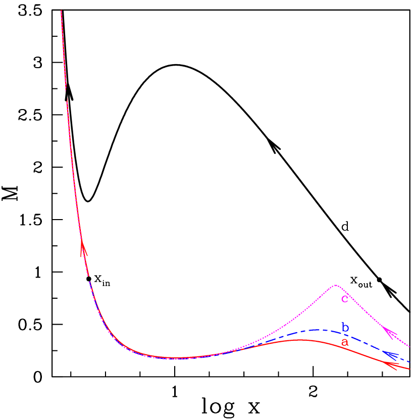
Figure 1: Radial dependence of Mach number ($M=\upsilon/a$) of the accreting matter for different values of angular momentum ($\lambda_{\rm edge}$) at the outer edge $x_{\rm edge}=500$ where $\beta_{\rm edge}=3500$, $\alpha_{B}=0.023$ and $\dot{m}=0.002$. Thin solid and short-long-dashed curves represent the results for $\lambda_{\rm edge}=5.6225$ and $3.6618$, respectively. For the same set of outer edge parameters, the minimum angular momentum that provides the accretion solution passing through the inner sonic is identified as $\lambda^{\rm min}_{\rm edge}=2.6654$ (dotted curve). When $\lambda_{\rm edge}<\lambda^{\rm min}_{\rm edge}$, accretion solutions pass through the outer sonic point only (thick solid curve) where $\lambda_{\rm edge}=2.2183$. In the figure, the locations of the inner sonic point ($x_{\rm in}$) and outer sonic point ($x_{\rm out}$) are marked and arrows indicate the direction of the flow motion towards the black hole. See text for details.

In Fig. 1, we present variation of Mach number $(M=\upsilon/a)$ versus logarithmic radial distance ($x$). The solid curve, denoted by ‘a’, depicts a global accretion solution passing through the inner sonic point $x_{\rm in}=2.4242$ with angular momentum $\lambda_{\rm in}=1.740$, $\beta_{\rm in}=19.0$, $\alpha_{B}=0.023$ and $\dot{m}=0.002$, respectively, and connects the BH horizon with the outer edge of the disc $x_{\rm edge}$, where we note the values of the flow variables $\lambda_{\rm edge}=5.6225$, $\beta_{\rm edge}=3500$, $\upsilon_{\rm edge}=0.00275$, $a_{\rm edge}=0.03726$ at $x_{\rm edge}=500$. In another way, we can obtain the same solution when the integration is carried out towards the black hole starting from the outer edge of the disc ($x_{\rm edge}$) with the noted boundary values. Hence, the above result necessarily describes the solution of an accretion flow that starts its journey from $x_{\rm edge}=500$ and crosses the inner sonic point at $x_{\rm in}=2.4242$ before crossing the event horizon. The arrow displays the direction of the flow. Now, we decrease $\lambda_{\rm edge}=3.6618$ holding all the other values of the flow variables same at $x_{\rm edge}=500$ and attain the global transonic solution by appropriately tuning the values of $\upsilon_{\rm edge}=0.00467$ and $a_{\rm edge}=0.03381$. The solution is denoted as ‘b’. Here, the values of $\upsilon_{\rm edge}$ and $a_{\rm edge}$ are further needed to start the integration as the sonic point is not identified a priori. Following this approach, we determine the minimum value of angular momentum at the outer edge $\lambda_{\rm edge}^{\rm min}=2.6654$, below this value accretion solution fails to pass through the inner sonic point. Accretion solution which corresponds to the minimum $\lambda_{\rm edge}^{\rm min}$ is illustrated by the dotted curve and marked as ‘c’. The streamlines namely ‘a-c’ depict solutions similar to the solution of advection dominated accretion flow around black holes (Narayan, Kato & Honma 1997; Oda et al. 2007). However, yet another important class of solutions stay unexamined which we deal with in this work. As $\lambda_{\rm edge}^{\rm min}$ is decreased further, such as $2.2183$, accretion solution changes its character and passes through the outer sonic point ($x_{\rm out}=300.89$) instead of inner sonic point ($x_{\rm in}$) with angular momentum $\lambda_{\rm out}=2.0499$, $\beta_{\rm out}=2283.02$ which is indicated by the thick solid line marked as ‘d’. In the context of magnetically supported accretion disc, there are only few studies of accretion solution passing through the outer sonic points (Sarkar & Das 2015, 2016; Sarkar et al. 2018). Solutions specifically of this kind are appealing as they are likely to possess centrifugally supported shock waves. The existence of shock wave in an accretion flow has profound significance as it satisfactorily characterizes the spectral and temporal behaviour of numerous black hole sources (Molteni el al. 1999, Rao et al. 2000, Okuda et al. 2004, 2008, Das et al. 2014; Nandi et al. 2012; Aktar et al. 2015, 2017; Iyer, Nandi & Mandal 2015, Suková & Janiuk 2015, Suková et al. 2017). Thus, the present effort aims to explore the properties of magnetically supported accretion solutions that possess shock waves.

3.2 Shock induced global accretion solution

Figure 2: A complete global accretion solution containing shock ($x_{s}=36.60$) is depicted along with outer ($x_{\rm out}$) and inner ($x_{\rm in}$) sonic points. Inflow parameters at the outer edge are same as case ‘d’ of Fig. 1. See text for details.

In Fig. 2, we present a composite global accretion solution containing shock wave where the flow transits the sonic location multiple times. Inflowing matter at the outer edge starts accreting towards the black hole subsonically with the boundary values same as the case ‘d’ of Fig. 1. The flow crosses the outer sonic point located at $x_{\rm out}=300.89$ and becomes supersonic. When the rotating matter advances further, it experiences virtual barrier caused by the centrifugal repulsion and begins piling up there. The process persists until at some point, shock formation is triggered when the shock conditons are satisfied and this leads to a discontinuous transition of the flow variables. This is because when dynamically possible, shock is thermodynamically preferred accretion solution since the post-shock matter possesses high entropy content (Becker & Kazanas 2001). For a dissipative accretion flow, the expression of the entropy-accretion rate in the flow is obtained as (Chakrabarti 1996; Sarkar et al. 2018),

$$\dot{\cal{M}}(x)\propto\left(\frac{\beta}{1+\beta}\right)^{n}a^{(2n+1)}\upsilon x^{3/2}(x-1).$$

In the absence of any dissipative processes like viscosity and/or radiative cooling, $\dot{\cal{M}}$ remains constant throughout the flow except at the shock.

In an accretion flow, shock transition is governed by the conservation laws of mass, momentum, energy and magnetic field (Sarkar & Das 2016, and reference therein). Across the shock front, these laws are clearly given as the continuity of (a) mass flux (${\dot{M}}_{-}={\dot{M}_{+}}$) (b) the momentum flux ($W_{-}+\Sigma_{-}\upsilon^{2}_{-}=W_{+}+\Sigma_{+}\upsilon^{2}_{+}$) (c) the energy flux (${\cal E_{-}}={\cal E_{+}}$) and (d) the magnetic flux ($\dot{\Phi}_{-}=\dot{\Phi}_{+}$) across the shock. Here, the quantities with subscripts ‘-’ and ‘+’ refer to values before and after the shock, respectively. While doing so, we inherently consider the shock to be thin and non-dissipative. The energy flux of the flow in the presence of a magnetic field is given by (Fukue 1990; Samadi et al. 2014),

$$\mathcal{E}=\frac{\upsilon^{2}}{2}+\frac{a^{2}}{\gamma-1}+\frac{\lambda^{2}(x)}{2x^{2}}-\frac{1}{2(x-1)}+\frac{<B_{\phi}^{2}>}{4\pi\rho}$$

In the immediate post-shock region, the flow becomes subsonic because of conversion of pre-shock kinetic energy in to the thermal energy. Hence, the post-shock matter becomes hot and dense. Subsonic post-shock matter continues its journey towards the BH because of gravitational attraction. It gains its radial velocity and consequently passes through the inner sonic point smoothly in order to satisfy the supersonic inner boundary condition before entering the event horizon. In Fig. 2, we present the variation of Mach number with the logarithmic radial distance. Thick curve refers to the accretion solution passing through the outer sonic point that can in principle enter in to the black hole directly. Interestingly, on the way towards the black hole, when the shock conditions are satisfied, flow makes discontinuous transition from the supersonic branch to the subsonic branch avoiding thick dot-dashed part of the solution. In the plot, the joining of the supersonic pre-shock flow with the subsonic post-shock flow is marked by the vertical arrow and the thin solid line denotes the inner part of the solution representing the post-shock flow. The overall direction of the flow motion during accretion towards black hole is indicated by the arrows.

3.3 Shock dynamics and shock properties

Here, we explore the dynamics of shock location as a function of the dissipation parameters ($\beta_{\rm edge}$ and/or $\dot{m}$) for flows where initial parameters are held fixed. In Fig. 3, matter is injected subsonically at the outer edge of the disc, $x_{\rm edge}=500$, with local specific energy, $\mathcal{E}_{\rm edge}=9.4855\times 10^{-4}$, local angular momentum, $\lambda_{\rm edge}=2.2460$ and viscosity, $\alpha_{B}=0.023$. When flow at $x_{\rm edge}=500$ is injected with accretion rate $\dot{m}=0.0001$ and plasma $\beta_{\rm edge}=3500$, the flow suffers shock transition at $x_{s}=246.62$. This result is represented in the figure by solid curve where vertical arrow represents the shock location. Next we increase the accretion rate to $\dot{m}=0.004$, holding rest of flow parameters fixed at $x_{\rm edge}$ and notice that the shock front moves closer to the horizon at $x_{s}=71.08$. This result is denoted using dotted curve where the dotted vertical arrow indicates the shock transition. Increase of $\dot{m}$ obviously augments the cooling rate of the flow. Since density and temperature of the flow undergo a catastrophic jump in the post-shock corona (PSC), effect of cooling in the PSC is intensified compared to the pre-shock flow. This reduces the post-shock thermal pressure and thus the shock moves closer to the black hole to maintain pressure balance across it. Additionally, we fix $\beta_{edge}=200$ and $\dot{m}=0.004$ maintaing the other flow parameters unchanged at $x_{\rm edge}$ and observe the shock to form at $x_{s}=26.98$. We represent this result by dashed curve where dashed vertical line denotes the shock location as before. Decrease in $\beta_{edge}$ indicates the increase of magnetic fields in the accretion flow that augments the Maxwell stress, thus enhancing the angular momentum transport from the inner to the outer region in the disc. Thus the centrifugal repulsion at the PSC weakens. Furthermore, decrease of $\beta_{\rm edge}$ ultimately enhances the synchrotron cooling efficiency as well. Consequently, the collective effects of both the physical processes drive the shock front even further towards the horizon. This highlights the important role played by $\beta_{edge}$ in deciding the dynamics of shock location, apart from the role played by $\dot{m}$.

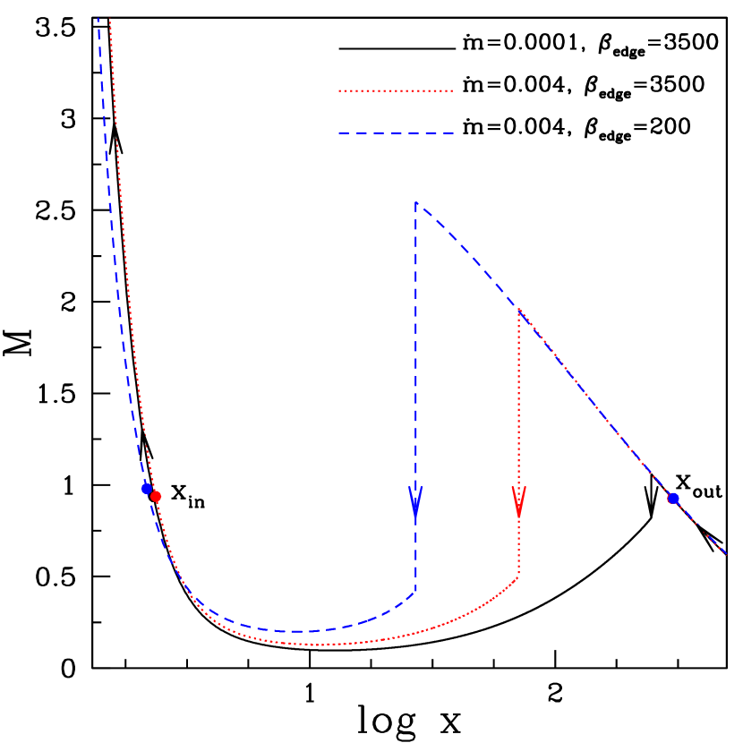
Figure 3: Variation of Mach number as function of logarithmic radial distance. Flows are injected from the outer edge $x_{\rm edge}=500$ with energy $\cal{E}_{\rm edge}$ = $9.4855\times 10^{-4}$, angular momentum $\lambda_{\rm edge}=2.2460$ and viscosity $\alpha_{B}=0.023$. Solid, dotted and dashed curves depict the results obtained for ($\dot{m},\beta_{\rm edge})$ = $(10^{-4},3500),(0.004,3500)$ and $(0.004,200)$, respectively. Vertical arrows indicate the corresponding shock transitions positioned at $x_{s}=246.62$ (solid), $x_{s}$ = 71.08 (dotted) and $x_{s}$ = 26.98 (dashed). See text for details.

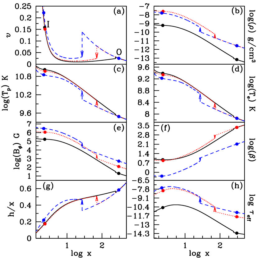
Figure 4: Variation of (a) radial velocity, (b) density in $g/cm^{3}$ , (c) proton temperature, (d) electron temperature, (e) strength of magnetic field, (f) ratio of gas pressure to magnetic pressure, (g) disc scale height ($h/x$) and (h) effective optical depth as function of logarithmic radial coordinate. Results plotted with solid, dotted and dashed curves correspond to the accretion solution depicted in Fig. 3. Filled circles represent the sonic points where the closer one is the inner sonic point and the furthest one is the outer sonic point. Vertical arrows indicate the shock position. See text for details

In Fig. 4, we demonstrate the vertically averaged accretion disc structure corresponding to the solutions considered in Fig. 3. In every panel, we depict the variation of a flow variable with logarithmic radial distance, where vertical arrows point out the shock transition. In Fig. 4(a), we plot the radial velocity profile ($\upsilon$) of the accretion flow. As anticipated, $\upsilon$ increases with the decrease of radial coordinate before it experiences a shock transition. After the shock transition $\upsilon$ drops to a subsonic value and again increases steadily in the PSC. Ultimately, flow enters the event horizon with velocity of the order of speed of light after crossing the inner sonic point. Here, solid, dotted and dashed curves exhibit results for ($\dot{m}$, $\beta_{\rm edge}$) = ($10^{-4}$, $3500$), ($0.004$, $3500$) and ($0.004$, $200$), respectively. We demonstrate the density profile of the flow in Fig. 4(b), where, we find an increase of density directly after the shock transition in each case. This occurs due to the decline of radial velocity at PSC, eventually preserving the conservation of mass flux across the shock front. The general trend of density profile corresponding to $\dot{m}=0.004$ is higher compared to the case of $\dot{m}=10^{-4}$ just because the large $\dot{m}$ signifies higher mass inflow at the outer edge. In Fig. 4(c), the proton temperature profile ($T_{p}$) is shown. During the shock transition, supersonic pre-shock flow is turned in to subsonic flow, and thereby, greater part of the kinetic energy of the infalling matter is converted to the thermal energy at PSC. This ultimately causes heating of the PSC as revealed by the rise of post-shock temperature profile. Additionally, when $\dot{m}$ rises, radiative cooling is more effective at PSC that explains the reduction of $T_{p}$ as clearly visible in the vicinity of the event horizon. Further, we notice that the decrease of $\beta_{\rm edge}$ necessarily displays the decrease of temperature profile of the flow. Fig. 4(d) shows the variation of electron temperature ($T_{e}$) with logarithmic radial distance. Since we have assumed the electron temperature to be estimated using proton temperature as $T_{e}\sim 0.023T_{p}$, the radial variation of $T_{e}$ follows the same trend as $T_{p}$. Importantly, since the radiative cooling is mostly effective at the inner part of the disc (due to high density, temperature and magnetic field), the synchrotron cooling is seen to be significantly effective in this region leading to decrease in $T_{e}$ profile. In Fig. 4(e), we show the variation of toroidal magnetic field ($B_{\phi}$) with logarithmic radial distance. $B_{\phi}$ increases radially as the flow approaches the BH because of increase of magnetic flux as matter approaches the event horizon. Compression of flow in the post-shock region causes the magnetic field strength to increase after the shock because of the conservation of magnetic flux ($\dot{\Phi}$) across the shock. Increase of accretion rate in the flow increases $B_{\phi}$ (through gas pressure) which in turn enhances angular momentum transport and pushes the shock front towards the BH. We present the radial variation of plasma $\beta$ profile in Fig. 4(f). We observe that $\beta$ decreases as the flow approaches to the horizon. Furthermore, $\beta$ drops sharply across the shock that renders the PSC into magnetically dominated. The radial variation of the vertical scale-height ($h/x$) is presented in Fig. 4(g). The validity of the thin disc approximation is found to hold all throughout from the outer edge to the horizon, in spite of the presence of shock transition. Lastly, in Fig. 4(h), we plot the variation of effective vertical optical depth, $\tau_{\rm eff}=\sqrt{\tau_{\rm es}\tau_{\rm syn}}$ (Rajesh & Mukhopadhyay 2010) where, $\tau_{\rm es}$ represents the scattering optical depth given by $\tau_{\rm es}=\kappa_{\rm es}\rho h$ and the electron scattering opacity, $\kappa_{\rm es}$, is taken to be $\kappa_{\rm es}=0.38~{}{\rm cm}^{2}{\rm g}^{-1}$. Here, $\tau_{\rm syn}$ denotes the absorption effect arising due to thermal processes and is given by $\tau_{\rm syn}=\left(hq_{\rm syn}/4\sigma T_{e}^{4}\right)\left(2GM_{\rm BH}/c^{2}\right)$ (Rajesh & Mukhopadhyay 2010) where, $q_{\rm syn}$ is the synchrotron emissivity (Shapiro & Teukolsky 1983) and $\sigma$ is the Stefan-Boltzmann constant. We observe that the optical depth of PSC is consistently greater than the pre-shock region because the density of post-shock region is higher (see, Fig. 4b). Moreover, the global variation of the optical depth for augmented accretion rate stays higher. In addition, despite of a steep density profile, PSC flow is found to remain optically thin ($\tau<1$). This instinctively leads to the conclusion that there is a significant possibility of escaping hard radiations from the PSC.

Fig. 5, demonstrates the different shock properties as a function of accretion rate ($\dot{m}$) for flows injected from a fixed outer edge as $x_{\rm edge}=500$ with $\beta_{\rm edge}$ = 3500, energy $\cal{E}_{\rm edge}$ = $9.4855\times 10^{-4}$ and viscosity $\alpha_{B}$ = 0.023. In the upper panel (Fig. 5a), the variation of shock position is shown for three different values of angular momentum ($\lambda_{\rm edge}$) at $x_{\rm edge}$. The solid, dotted and dashed curves correspond to flows injected with angular momentum $\lambda_{\rm edge}$ = $2.2120$, $2.2290$ and $2.2460$ respectively. Evidently, we find that a wide range of $\dot{m}$ supports shock induced global accretion solutions. For a given $\lambda_{\rm edge}$, the location of shock advances towards the horizon with the increment of accretion rate ($\dot{m}$). With the rise of accretion rate the efficiency of radiative cooling is enhanced and the flow loses energy during accretion. Loss of energy causes drop in post-shock thermal pressure thus pushing the shock front closer to the horizon in order to maintain pressure balance across the shock. When accretion rate exceeds its critical value ($\dot{m}^{\rm cri}$), standing shock no longer form as the shock conditions are not fulfilled. This clearly suggests that the likelihood of shock formation reduces with the increase of $\dot{m}$. It should be noted that ($\dot{m}^{\rm cri}$) does not have a global value, rather it primarily depends on the accretion flow parameters. Interestingly enough, when $\dot{m}>(\dot{m}^{\rm cri})$, flow can have oscillatory shocks, however, the investigation of non-steady shock properties are out of scope of the present work. Such type of oscillation of the post-shock region has been shown by Molteni et al. (1996). In addition, for a given $\dot{m}$, shock front recedes from the horizon with the increase of $\lambda_{\rm edge}$. This is because the centrifugal barrier strengthens with the increase of $\lambda_{\rm edge}$. From this it is clear that shocks in accretion flow around black holes are centrifugally driven. It is evident from Fig. 5(a) that when $\lambda_{\rm edge}$ is decreased the range of $\dot{m}$ over which shock exists, decreases. When $\lambda_{\rm edge}$ will be decreased below the value $2.2120$, shocks will exist for still lower range of $\dot{m}$ and will finally cease to exist when $\lambda_{\rm edge}$ will be decreased beyond a critical limit because standing shock will fail to form. It is previously noted that the shock

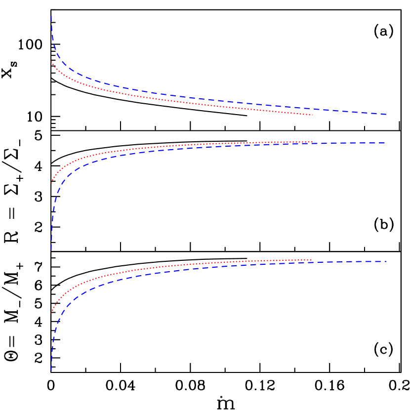
Figure 5: Variation of (a) shock location $x_{s}$, (b) compression ratio $R$, and (c) shock strength $\Theta$ as function of $\dot{m}$ for flows injected from $x_{\rm edge}$ = 500 with $\alpha_{B}$ = 0.023, $\beta_{\rm edge}=3500$ and $\cal{E}_{\rm edge}$ = $9.4855\times 10^{-4}$. Solid, dotted and dashed curves represent the results corresponding to $\lambda_{\rm edge}$ = $2.2120$, $2.2290$ and $2.2460$, respectively. See text for details.

compression causes the density and temperature of the PSC to increase. Furthermore, the spectral properties of an accretion disc are directly determined by the density and temperature distribution of the flow. Hence, it is imperative to estimate the amount of density and temperature boost across the shock transition. For this, we first evaluate the compression ratio which is defined as the ratio of the vertically averaged post-shock density to the pre-shock density ($R=\Sigma_{+}/\Sigma_{-}$) and plot it as function of $\dot{m}$ in Fig. 5b. We retain the flow parameters chosen in Fig. 5a. For a given $\lambda_{\rm edge}$, $R$ is seen to grow monotonicaly with the increase of $\dot{m}$. That is so because the shock is pushed closer to the horizon with the increase of $\dot{m}$ boosting the density compression and resulting in increase of compression ratio. Oppositely, for a given $\dot{m}$, when $\lambda_{\rm edge}$ is increased, the centrifugal barrier strengthens and shock recedes away form the horizon leading to decrease in the post-shock compression. When $\dot{m}>(\dot{m}^{\rm cri})$, since shock cease to exist, we observe a cut-off in the compression ratio in all the cases. Next, we compute the shock strength ($\Theta$) defined as the ratio of pre-shock Mach number ($M_{-}$) to the post-shock Mach number ($M_{+}$) which basically measures the temperature jump across the shock. In Fig. 5(c), we plot the variation of $\Theta$ as a function of accretion rate $\dot{m}$ for the same injection parameters as in Fig. 5(a). We observe that the response of $\Theta$ on the increase of $\dot{m}$ is identical to $R$ as represented in Fig. 5(b).

4 Conclusions

In this work, we demonstrate that the synchrotron cooling plays an important role in a magnetized accretion disc around black holes. Efforts are still ongoing to study the origin of viscosity and the exact mode of angular momentum transport in accretion discs by several authors (Menou 2000, Balbus 2003, Becker & Subramanian 2005, Kaufmann et al. 2007, King et al. 2007, Guan & Gammie 2009, Hopkins & Quataert 2011, Kotko & Lasota 2012). Hence, we rely on the numerical simulation results of Machida et al. (2006). Following Machida et al. (2006), we assume the x$\phi$ -component of the Maxwell stress to be proportional to the total pressure. We find that such a flow is transonic and passes through the sonic point multiple times giving rise to the phenomenon of shocks in the accretion flow. Global accretion solutions of magnetically supported accretion discs around stationary black holes have been carried out by Oda et al. (2007, 2012). These works show the accretion solutions passing through a single sonic point only and ignore the possibility of multiple sonic points in the flow. Thus the solutions presented by Oda et al. (2007, 2012) are a subset of the generalized accretion solutions studied in this work. In Sarkar & Das (2016), the magnetic field strength was assumed to be moderate throughout the flow. However the present work has no such restrictions and shock solutions have been shown to be present in the disc when the inner region is magnetically dominated ($\beta<1$) as well (Fig. 4f). We make a detailed study of the effects of the dissipation variables, namely accretion rate ($\dot{m}$) and magnetic parameter $\beta$ on the global accretion solutions. We find that increase in radiative loss due to increase of cooling and strength of magnetic field removes a significant thermal pressure from the inflow and as the dissipation increases, the shock location shifts towards the black hole to maintain the pressure balance across it. When the dissipation is reached its critical value, standing shocks can no longer form. Such a study is highly important since the dissipation parameters are likely to influence the spectral and timing properties of the radiation emitted from the disc. We have studied the effect of cooling on the shock dynamics. For a flow strating from a large distance with a given set of outer edge conditions, there exists a cut-off in accretion rate, beyond which, steady shock solutions cannot exist, as in Fig. 5. Beyond the critical limit, unsteady, oscillating shocks are possible (Das et al. 2014). We ignore the formation of such oscillating shocks since their study is out of the scope of the present work.

Finally, we point out the limitations of the present work. In this paper, the adiabatic index has been considered to be constant throughout the flow instead of calculating it self-consistently. Also, the black hole in this paper has been considered to be non-rotating. Apart from plasma $\beta$, the spin of the black hole is also expected to affect the dynamics of shocks. We would like to consider the above issues in the future works.

References

- [1] Aktar, R., Das, S., Nandi, A. 2015, MNRAS, 453, 3414.
- [2] Aktar, R., Das, S., Nandi, A., Sreehari, H. 2017, MNRAS, 471, 4806.
- [3] Balbus, S., Hawley, J. F. 1991, ApJ, 376, 214.
- [4] Balbus, S. 2003, ARA&A, 41, 555.
- [5] Becker, P. A., Kazanas, D. 2001, ApJ, 546, 429.
- [6] Becker, P. A., Subramanian, P. 2005, ApJ, 622, 520.
- [7] Beckwith, K., Hawley, J. F., Krolik, J. H. 2008, ApJ, 678, 1180.
- [8] Blandford, R. D., Znajek, R. L. 1977, MNRAS, 179, 433.
- [9] Chakrabarti, S. K. 1989, ApJ, 347, 365.
- [10] Chakrabarti, S. K. 1990, MNRAS, 243, 610.
- [11] Chakrabarti, S. K. 1996, ApJ, 464, 664.
- [12] Chakrabarti, S. K. 1999, A&A, 351, 185
- [13] Chakrabarti, S. K., Das, S. 2004, MNRAS, 349, 649.
- [14] Chang, K. M., Ostriker, J. P. 1985, ApJ, 288, 428.
- [15] Chattopadhyay, I., Chakrabarti, S. K. 2002, MNRAS, 333, 454.
- [16] Chattopadhyay, I., Chakrabarti, S. K. 2011, IJMPD, 20, 1597.
- [17] Das, S., Chattopadhyay, I., Chakrabarti, S. K. 2001a, ApJ, 557, 983.
- [18] Das, S., Chattopadhyay, I., Nandi, A., Chakrabarti, S. K. 2001b, A&A, 379, 683.
- [19] Das, S. 2007, MNRAS, 376, 1659.
- [20] Das, S., Chattopadhyay, I., Nandi, A., Molteni, D. 2014, MNRAS, 442, 251.
- [21] De Villiers, J.-P., Hawley, J. F., Krolik, J. H., Hirose, S. 2005, ApJ, 620, 878.
- [22] Fukue, J. 1987, PASJ, 39, 309.
- [23] Fukue, J. 1990, PASJ, 42, 793.
- [24] Fukumura K., Tsuruta S. 2004, ApJ, 611, 964.
- [25] Gierliński, M., Newton, J. 2006, MNRAS, 370, 837.
- [26] Guan, X., Gammie, C. F. 2009, ApJ, 697, 1901.
- [27] Hawley, J. F. 2000, ApJ, 528, 462.
- [28] Hawley, J. F. 2001, ApJ, 554, 534.
- [29] Hawley, J. F., Krolik, J. H. 2001, ApJ, 548, 348.
- [30] Hawley, J. F., Krolik, J. H. 2002, ApJ, 566, 164.
- [31] Hirose, S., Krolik, J. H., De Villiers, J. P., Hawley, J. F. 2004, ApJ, 606, 1083.
- [32] Hirose, S., Krolik, J. H., Stone, J. M. 2006, ApJ, 640, 901.
- [33] Hopkins P. F., Quataert E. 2011, MNRAS, 415, 1027.
- [34] Ichimaru, S. 1977, ApJ, 214, 840.
- [35] Igumenshchev, I. V., Narayan, R., & Abramowicz, M. A. 2003, ApJ, 592, 1042.
- [36] Iyer, N., Nandi, A., Mandal, S. 2015, ApJ, 807, 108.
- [37] Johansen, A., Levin, Y. 2008, A&A, 490, 501.
- [38] McKinney, J. C., Gammie, C. F. 2004, ApJ, 611, 977.
- [39] Kato, Y., Mineshige, S., Shibata, K. 2004, ApJ, 605, 307.
- [40] Kaufmann T., Mayer L., Wadsley J., Stadel J. and Moore B. 2007, MNRAS, 375, 53.
- [41] King A. R., Pringle J. E. & Livio M. 2007, MNRAS, 376, 1740.
- [42] Koide S., Shibata K., Kudoh T., Meier D. L. 2002, Science, 295, 1688.
- [43] Kotko, I., Lasota, J.-P. 2012, A&A, 545, A115.
- [44] Krolik, J. H., Hirose, S., Blaes, O. 2007, ApJ, 664, 1045.
- [45] Landau L. D., Lifshitz E. D. 1959, Fluid Mechanics (New York, Pergamon).
- [46] Lebedev, S. V., Ciardi, A., Ampleford, D. J., et al. 2005, MNRAS, 361, 97.
- [47] Lu, J. F., Yu, K. N., Yuan, F., Young, E. C. M. 1997, A&A, 321, 665.
- [48] Lu, J. F., Yuan, F. 1998, MNRAS, 295, 66.
- [49] Machida, M., Matsumoto, R. 2003, ApJ, 585, 429.
- [50] Machida, M., Nakamura, K. E., Matsumoto, R. 2006, PASJ, 58, 193.
- [51] Mandal, S., Chakrabarti, S. K. 2005, Ap&SS, 297, 269.
- [52] Matsumoto, R., Kato, S., Fukue, J., Okazaki, A. T. 1984, PASJ, 36, 71.
- [53] McKinney, J., Blandford, R. 2009, MNRAS, 394, L126.
- [54] Menou, K. 2000, Sci, 288, 2022.
- [55] Molteni, D., Sponholtz, H., Chakrabarti, S. K. 1996, ApJ, 457, 805.
- [56] Molteni D., Toth G., Kuznetsov O. A. 1999, ApJ, 516, 411.
- [57] Narayan, R., Yi, I. 1995, ApJ, 452, 710.
- [58] Narayan, R., Kato, S., Honma, F. 1997, ApJ, 476, 49.
- [59] Nandi, A., Debnath, D., Mandal, S., Chakrabarti, S. K. 2012, A&A, 542, 56.
- [60] Oda, H., Machida, M., Nakamura, K. E., Matsumoto, R. 2007, PASJ, 59, 457.
- [61] Oda, H., Machida, M., Nakamura, K. E., Matsumoto, R. 2010, ApJ, 712, 639.
- [62] Oda, H., Machida, M., Nakamura, K. E., Matsumoto, R., Narayan, R. 2012, PASJ, 64, 15.
- [63] Okuda T., Teresi V., Toscano E., Molteni D. 2004, PASJ, 56, 547.
- [64] Okuda, T., Teresi, V., Molteni, D. 2008, AIP Conference Proceedings, vol. 968, p. 417.
- [65] Paczyński, B., Wiita, P. J. 1980, A&A, 88, 23.
- [66] Papaloizou, J. C. B., Terquem, C. 1997, MNRAS, 287, 771.
- [67] Parker, E. N. 1966, ApJ, 145, 811.
- [68] Pudritz, R. E., Norman, C. A. 1986, Can. J. Phys., 64, 501.
- [69] Rajesh, S. R., Mukhopadhyay B. 2010, MNRAS, 402, 961.
- [70] Rao A. R., Yadav J. S., Paul B. 2000, ApJ, 544, 443.
- [71] Samadi, M., Abbassi, S., Khajavi, M. 2014, MNRAS, 437, 3124.
- [72] Sarkar, B., Das, S. 2015, ASInC, 12, 91.
- [73] Sarkar, B., Das, S. 2016, MNRAS, 461, 190.
- [74] Sarkar, B., Das, S., Mandal, S. 2018, MNRAS, 473, 2415.
- [75] Shakura, N. I., Sunyaev, R. A. 1973, A&A, 24, 337.
- [76] Shapiro, S. L., Teukolsky, S. A. 1983, Black Holes, White Dwarfs and Neutron Stars: The Physics of Compact Objects (New York, Wiley).
- [77] Shibata, K., Tajima, T., & Matsumoto, R. 1990, ApJ, 350, 295.
- [78] Singh, C. B., Chakrabarti, S. K. 2011, MNRAS, 410, 2414.
- [79] Spruit, H. C., & Uzdensky, D. A. 2005, ApJ, 629, 960.
- [80] Suková P., Janiuk A. 2015, MNRAS, 447, 1565.
- [81] Suková P., Charzyński, S., Janiuk A. 2017, MNRAS, 472, 4327.
- [82] Ustyugova, G. V., Koldoba, A. V., Romanova, M. M., Chechetkin, V. M., & Lovelace, R. V. E. 1999, ApJ, 516, 221.
- [83] Yuan, F. 2001, MNRAS, 324, 119.