Solution of the sign problem in the Potts model
at fixed fermion number

Abstract

We consider the heavy-dense limit of QCD at finite fermion density in the canonical formulation and approximate it by a 3-state Potts model. In the strong coupling limit, the model is free of the sign problem. Away from the strong coupling, the sign problem is solved by employing a cluster algorithm which allows to average each cluster over the ${\mathbb{Z}}(3)$ sectors. Improved estimators for physical quantities can be constructed by taking into account the triality of the clusters, that is, their transformation properties with respect to ${\mathbb{Z}}(3)$ transformations.

1 Introduction

At present, the non-perturbative properties of QCD at finite baryon density can not be studied from first principles, because the theory suffers from a fermion sign problem as soon as the baryon chemical potential $\mu$ is nonzero. More precisely, the fluctuating sign of the fermion determinant in the path integral at nonzero $\mu$ prevents the interpretation of the Boltzmann factor as a probability measure and hence renders importance sampling methods such as Monte Carlo (MC) simulations of lattice QCD inapplicable. One common approach to the problem is to include the fluctuating sign of the Boltzmann factor in the measured observables. While this is in principle a valid procedure, in practice it is bound to fail because the severe cancellations require the statistics to grow exponentially with the space-time volume of the lattice.

Nevertheless, it turns out that in some limiting cases the fermion sign problem is mild or even absent. One such situation concerns lattice QCD in the so-called heavy-dense limit in the canonical formulation at infinitely strong coupling. In the heavy-dense limit, the fermion contributions to the path integral are encoded in Polyakov loops associated with static quarks and antiquarks propagating in time. In the strong coupling limit, the Polyakov loops decouple in the effective action and the global ${\mathbb{Z}}(3)$ symmetry of QCD at zero density is promoted to a local one. This in turn allows to project the propagating quark states in the canonical formulation exactly onto mesonic and baryonic states localized on single sites. The contributions of those states to the path integral have a phase which is zero or extremely small, hence allowing MC calculations. Despite this happy state of affairs in the strong coupling limit, as soon as the coupling is tuned away from this limit, the sign problem strikes back with vengeance – it swamps away any coherent contribution from the colour neutral states and consequently renders MC simulations impossible.

However, the physical picture emerging in the strong coupling limit indicates how the relevant fermionic contributions to the path integral, being physical and having small or even zero phases, may look like away from infinitely strong coupling. In fact, one may speculate that whenever the quarks and antiquarks form mesonic and baryonic clusters, within which the Polyakov loops fluctuate in conjuction, a coherent physical contribution should arise, very similar to what happens in the strong coupling limit. In order to substantiate this speculation and study the mechanism in more detail, in this paper we simplify the problem further and consider a system in which the gauge dynamics is replaced by that of the ${\mathbb{Z}}(3)$ Potts model and the Polyakov loops are represented by the Potts spins $z\in{\mathbb{Z}}(3)$ [1, 2, 3, 4]. For the canonical formulation of this model, where the quarks are represented in terms of quark occupation numbers, we are able to devise a cluster algorithm that solves the fermion sign problem completely, in a similar way as the cluster algorithm in [5] for the grand-canonical formulation with a finite chemical potential. However, in the canonical situation described in this paper, the solution has a clear and very intriguing physical interpretation in terms of the quark occupation numbers, very much in line with the physical picture that emerges for QCD in the heavy-dense and strong coupling limit as described above.

In the cluster formulation it turns out that the only physical, nonzero contributions to the canonical partition functions are exclusively from clusters which contain exactly a multiple of three quarks. The weights of these clusters are invariant under ${\mathbb{Z}}(3)$ transformations and we denote the corresponding clusters as triality-0 clusters. Clusters with one or two additional quarks are denoted as triality-1 and triality-2 clusters, respectively, refering to the transformation properties of their weights with respect to ${\mathbb{Z}}(3)$ transformations. Their total contributions to the canonical partition functions exactly vanish, but they contribute to observables which consist of nonzero-triality quark fields.

The clusters which are formed in the canonical picture allow for a straightforward physical interpretation. The triality-0 clusters containing a nonzero number of quarks represent baryon or multi-baryon states. While the quarks can move freely within the cluster, of course always respecting the Pauli exclusion principle, they are nevertheless confined within the clusters. It is therefore obvious to interpret these clusters as baryon bags. Empty clusters on the other hand represent vacuum fluctuations of the underlying gauge degrees of freedom. In case we also allow antiquarks in the system, the triality-0 clusters may also contain mesons and represent all kinds of multi-baryon-multi-meson bags.

This physical picture is also useful to interpret the transition from the confined phase to the deconfined one. At low temperature and density, the clusters tend to be very small and form a dilute gas of hadrons, representing the system in the confined phase. When the temperature is increased, the clusters grow larger and start to percolate, at which point the system undergoes a first order phase transition into the deconfined phase. At even higher temperatures, one single cluster essentially fills the whole volume and the quarks can hence move freely within the whole volume.

Before moving on to work this picture out in full detail, it is useful to discuss the symmetry properties of the ${\mathbb{Z}}(3)$ Potts model at finite density. While the model at zero fermion density is invariant under global ${\mathbb{Z}}(3)$-symmetry transformations, this is no longer true at finite density. In that case the introduction of the chemical potential breaks the ${\mathbb{Z}}(3)$ symmetry explicitly. In contrast, in the canonical formulation the contributions from the static charges have definite transformation properties under ${\mathbb{Z}}(3)$ transformations, such that the contributions vanish unless the number of charges is a multiple of 3. As a consequence, the non-vanishing contributions are manifestly invariant under global ${\mathbb{Z}}(3)$-symmetry transformations.

The paper is organised as follows. Section 2 contains the definition of the ${\mathbb{Z}}(3)$ Potts model and its canonical formulation. In section 3 we introduce the bond formulation and describe the cluster algorithm for the canonical formulation, while in section 4 we construct improved estimators for various physical quantities such as the quark-antiquark, the quark-quark, the antiquark-antiquark and the 3-quark correlator, as well as the free energy of a single quark and of a single antiquark. A practical algorithm to sample the various sectors in configuration space based on the calculation of the multiplicities of quark configurations with subsequent reweighting is presented in section 5. Next, in section 6 we discuss the severity of the sign problem, while in section 7 we present a selection of simulation results, including an illustration of how the expected phase transition at very low fermion density manifests itself in the canonical setup. Finally, section 8 contains our conclusions, while some technical details are collected in the appendices.

2 The 3-dimensional ${\mathbb{Z}}(3)$ Potts model

In order to introduce the 3-dimensional ${\mathbb{Z}}(3)$ Potts model we follow [5] and approximate the grand-canonical partition function of QCD in the heavy-dense limit by

$$Z_{\text{GC}}(h)=\int{\cal D}z\,\exp(-S[z]+h\sum_{x}z_{x})$$ (1)

where the Potts spins $z_{x}\in{\mathbb{Z}}(3)$ are defined on discrete lattice points $x$ and stand for the Polyakov loop variables generated by the infinitely heavy quarks. The parameter $h=(2\kappa e^{\mu})^{\beta}$ refers to the hopping parameter $\kappa$, the chemical potential $\mu$ and the inverse temperature $\beta$ of the original theory. The precise form of the action can in principle be derived from QCD by integrating out all degrees of freedom except for the ${\mathbb{Z}}(3)$ phase of the Polyakov loop. In the Potts model $h$ plays the role of an external (magnetic) field which couples to the Potts spins and hence explicitly breaks the ${\mathbb{Z}}(3)$ symmetry present for a ${\mathbb{Z}}(3)$-invariant action $S[z]$ and $h=0$.

In the canonical formulation the partition function for $N_{Q}$ quarks can be written in the generic form

$$Z_{\text{C}}(N_{Q})=\sum_{\{n\}}\int{\cal D}z\,\exp(-S[z])\cdot\prod_{x}g[z_{x},n_{x}]\,.$$ (2)

Here the quark occupation numbers $n_{x}\in\{0,\ldots,n_{\text{max}}\}$ are collected in the quark configuration $n=\{n_{x}\}$ and the sum is over all quark configurations which fulfill $|n|\equiv\sum_{x}n_{x}=N_{Q}$. The finite maximal number of quarks $n_{\text{max}}$ on each site implements the Pauli exclusion principle. The fermionic weights $g[z_{x},n_{x}]$ can in principle be derived from QCD and in general also involve the anti-Polyakov loops $z_{x}^{*}$ and corresponding occupation numbers $\bar{n}_{x}$ for the antiquarks. Here we replace the fermionic weights by

$$g[z,n]=z^{n}\,.$$ (3)

For this case, the connection to the grand-canonical partition function in eq.(1) can be made explicit and it can be shown that the correspondence is exact for $h\ll 1$, i.e. at low densities. We refer to Appendix A for further details.

For the action $S[z]$ representing the pure gluon action we choose the standard nearest-neighbour Potts model interaction

$$S[z]=-\gamma\sum_{\langle xy\rangle}\delta_{z_{x},z_{y}}$$ (4)

where the sum is over all nearest-neighbour lattice sites. Note that the total action including the fermionic weights is manifestly complex and suffers from a sign problem just as in the grand-canonical formulation. However, the properties of the action under global ${\mathbb{Z}}(3)$ transformations ensure that

$$Z_{N_{Q}\neq 0\text{ mod }3}=0\,.$$ (5)

In the limit $\gamma\rightarrow 0$, corresponding to the strong coupling limit in QCD, the Potts spins fluctuate independently on each site and the global ${\mathbb{Z}}(3)$ transformation is promoted to a local one which hence enforces

$$n_{x}=0\text{ mod }3,\quad\forall x\qquad\text{('strong coupling limit' $\gamma\rightarrow 0$)}.$$ (6)

The fermionic weights then become trivial and the partition function simply counts the number of allowed quark configurations,

$$\lim_{\gamma\rightarrow 0}Z_{N_{Q}}=\sum_{\{n\}}\int{\cal D}z=3^{V}\cdot G(N_{Q}/3)\,.$$ (7)

In case the quark occupation number is restricted to $n_{x}\leq n_{\text{max}}=3$, the number of allowed quark configurations yields $G(N_{Q}/3)={{V}\choose{N_{Q}/3}}$.

3 Bond formulation and cluster algorithm

For finite gauge coupling the canonical partition function reads

$$Z_{N_{Q}}=\sum_{\{n\}}\int{\cal D}z\exp(\gamma\sum_{\langle xy\rangle}\delta_{z_{x},z_{y}})\prod_{x}z_{x}^{n_{x}}$$ (8)

and with the help of

$$e^{\gamma\cdot\delta_{z_{x},z_{y}}}=\sum_{b_{xy}=0}^{1}\left(\delta_{z_{x},z_{y}}\delta_{b_{xy},1}\left(e^{\gamma}-1\right)+\delta_{b_{xy},0}\right)$$ (9)

it can be written as

$$Z_{N_{Q}}=\sum_{\{n\}}\sum_{\{b\}}\int{\cal D}z\prod_{\langle xy\rangle}\left(\delta_{z_{x},z_{y}}\delta_{b_{xy},1}\left(e^{\gamma}-1\right)+\delta_{b_{xy},0}\right)\prod_{x}z_{x}^{n_{x}}$$ (10)

where the sum is over all bond configurations $b=\{b_{xy}\}$. For future reference we introduce a double bracket notation to abbreviate the sum over $\{b\}$, $\{n\}$ and ${\cal D}z$ weighted by the bond factors. For a generic quark number $N_{Q}=\sum_{x}n_{x}$ and a generic function $f(\{z_{x}\})$ we define

$$\llangle\prod_{x}z_{x}^{n_{x}}\cdot f(\{z_{x}\})\rrangle_{N_{Q}}=\sum_{\{n\}}\sum_{\{b\}}\int{\cal D}z\prod_{\langle xy\rangle}\left(\delta_{z_{x},z_{y}}\delta_{b_{xy},1}\left(e^{\gamma}-1\right)+\delta_{b_{xy},0}\right)\prod_{x}z^{n_{x}}\cdot f(\{z_{x}\})\,,$$ (11)

i.e., eq.(10) becomes

$$Z_{N_{Q}}=\llangle\prod_{x}z_{x}^{n_{x}}\rrangle_{N_{Q}}$$ (12)

Let us now consider for a moment the case $N_{Q}=0$ when there are no fermionic contributions through the Polyakov loops. From the expression above we read off that for a given spin configuration a bond $b_{xy}$ is occupied with probability $p(b_{xy}=1)=(1-e^{-\gamma})$ if the two neighbouring spins $z_{x}$ and $z_{y}$ are aligned, else it is empty ($b_{xy}=0$). The weight of such a bond configuration is then simply $W(\{b\})=(e^{\gamma}-1)^{N_{b}}$, where $N_{b}=\sum_{\langle xy\rangle}b_{xy}$ is the total number of occupied bonds, and it is independent of the orientation of the spins within the connected clusters of bonds. Hence, all spins within a cluster can be flipped into any of the three states independently of the spins in the other clusters. Up to here, this is just the well-known Swendsen-Wang cluster reformulation [6] of the Potts model. One can now integrate out the spins for a given bond configuration by summing over all possible combinations of cluster orientations, yielding

$$Z_{N_{Q}=0}=\llangle 1\rrangle_{N_{Q}=0}=\sum_{\{b\}}(e^{\gamma}-1)^{N_{b}}\cdot 3^{N_{C}}$$ (13)

where $N_{C}$ is the number of clusters for the given bond configuration. This is just the random cluster model representation of the Potts model as derived by Fortuin and Kasteleyn in [7]. Note that the integration over the spins is possible because the bond variables decouple the spin orientations of the clusters from each other, so that the integration over the spin degrees of freedom can be factorized over the clusters. This factorization is in fact the basis for the solution of the sign problem when the fermionic contributions are included.

In order to simulate the system according to the weights given in eq.(13), the bonds can be updated with a local algorithm as follows. A bond whose value does not change the number of clusters is activated with probability $p=1-e^{-\gamma}$. A bond which connects two clusters $C_{1}$ and $C_{2}$, which would otherwise be separate, is a bridging bond and therefore called a bridge in short. Activating a bridge decreases the number of clusters $N_{C}$ by one, and it is therefore done with a probability

$$p(C_{1},C_{2}\rightarrow C_{1}\cup C_{2})=\frac{e^{\gamma}-1}{e^{\gamma}+2}=\frac{1-e^{-\gamma}}{1+2e^{-\gamma}}\,,$$ (14)

while the bridge is deactivated with the probability

$$p(C_{1}\cup C_{2}\rightarrow C_{1},C_{2})=\frac{3}{e^{\gamma}+2}=\frac{3e^{-\gamma}}{1+2e^{-\gamma}}\,.$$ (15)

Hence, the update of a bond requires one to check whether the bond under consideration is a bridge or not. This is a well known, difficult problem in computational complexity theory and goes under the name fully-dynamic connectivity problem. For further details and our strategy to deal with the problem we refer to Appendix B.

For $N_{Q}>0$ we can include the fermionic contribution in our considerations by constructing an improved estimator for it. For an individual configuration the contribution $\prod_{x}z^{n_{x}}$ is in general complex, but its average over the subensemble of the $3^{N_{C}}$ configurations related by the ${\mathbb{Z}}(3)$ transformations of the individual clusters is rather simple. In the following we denote this subensemble average by $\langle\,\cdot\,\rangle_{3^{N_{C}}}$. We first observe that the total weight can be factorized into individual cluster weights $W_{0}(C)$,

$$\langle\prod_{x}z_{x}^{n_{x}}\rangle_{3^{N_{C}}}=\langle\prod_{C}\prod_{x\in C}z_{x}^{n_{x}}\rangle_{3^{N_{C}}}=\prod_{C}\langle\prod_{x\in C}z_{x}^{n_{x}}\rangle_{3}=\prod_{C}W_{0}(C)\,,$$ (16)

where by $\langle\,\cdot\,\rangle_{3}$ we denote the average over the three ${\mathbb{Z}}(3)$ orientations of a given cluster. This average can be calculated due to the fact that all spins in the cluster are aligned,

$$W_{0}(C)=\langle\prod_{x\in C}z^{n_{x}}\rangle_{3}=\langle z^{\sum_{x\in C}n_{x}}\rangle_{3}=\left\{\begin{array}[]{ll}1&\text{if }\sum_{x\in C}n_{x}=0\text{ mod }3,\\ 0&\text{else}.\end{array}\right.$$ (17)

Denoting the fermion number content of each cluster modulo 3 by

$$n_{C}=\sum_{x\in C}n_{x}\text{ mod }3\,,$$ (18)

the cluster weight simply becomes $W_{0}(C)=\delta_{n_{C},0}$. In the following we refer to $n_{C}$ as the triality of the cluster $C$. Consequently, all bond clusters can be classified according to their fermion content $n_{C}$, i.e. their triality. Clusters with nonzero triality $n_{C}=1$ or 2 have a vanishing contribution to the partition function, while clusters with zero triality $n_{C}=0$ contribute positively with weight 1. Hence, the partition function can now be written as

$$Z_{N_{Q}}=\llangle\prod_{x}z_{x}^{n_{x}}\rrangle_{N_{Q}}=\sum_{\{n\}}\sum_{\{b\}}(e^{\gamma}-1)^{N_{b}}\cdot 3^{N_{C}}\cdot\prod_{C}\delta_{n_{C},0}$$ (19)

where the sums are with respect to all bond and occupation number configurations (with $\sum_{x}n_{x}=N_{Q}$). The fermionic contribution $\prod_{x}z_{x}^{n_{x}}$ simply projects onto the sector of configurations containing only triality-0 clusters. Note that although the contributions to the partition function are now all positive, the expectation value of the fermionic contribution with respect to the full, unrestricted ensemble with fixed $N_{Q}$,

$$\langle\prod_{C}\delta_{n_{C},0}\rangle_{N_{Q}}=\frac{\llangle\prod_{x}z_{x}^{n_{x}}\rrangle_{N_{Q}}}{\llangle 1\rrangle_{N_{Q}}}\,,$$ (20)

can still be exponentially small, because the probability to find configurations without nonzero-triality clusters among all possible cluster and fermion number configurations can be exponentially small in the volume. In fact, it is easy to see that eq.(20) is just the expectation value of the complex phase in the modified real action ensemble and represents a measure for the severity of the sign problem. We refer to Sec. 6 for a more detailed discussion.

Nevertheless, the partition function can in principle be updated by directly operating on the bond variables and the fermion occupation numbers. Updates need to ensure that the system stays in the configuration space containing only triality-0 clusters. The bond update can be implemented as before with the cluster break-up probability in eq.(15) modified to

$$p(C_{1}\cup C_{2}\rightarrow C_{1},C_{2})=\frac{3}{e^{\gamma}+2}\cdot\delta_{n_{C_{1}},0}\cdot\delta_{n_{C_{2}},0}=\frac{3e^{-\gamma}}{1+2e^{-\gamma}}\cdot\delta_{n_{C_{1}},0}\cdot\delta_{n_{C_{2}},0}\,,$$ (21)

where the $\delta$-functions make sure that no clusters with nonzero triality are generated. Note that this step fulfills detailed balance since the situation involving the reverse step, i.e. connecting two clusters with at least one having nonzero triality, can never occur. Once the bond configuration is updated, the fermion occupation numbers can be updated locally by proposing to shift a fermion from site $x$ to one of its nearest-neighbour sites $y$. The shift is accepted with probability 1 as long as the fermion remains in the same cluster. Hops to sites which are already saturated are forbidden, as well as hops into a different cluster, since these would leave behind two clusters with nonzero triality. Hence, for two neighbouring sites $x$ and $y$ we have

$$p(n_{x},n_{y}\rightarrow n_{x}-1,n_{y}+1)=(1-\delta_{n_{x},0})(1-\delta_{n_{y},n_{\text{max}}})\cdot\delta_{C_{x},C_{y}}$$ (22)

where $C_{x}$ and $C_{y}$ denote the clusters containing the sites $x$ and $y$, respectively. Additional update steps can of course be envisaged and might be favourable with respect to efficiency of the algorithm. For example, one could let three fermions, i.e. a baryon, hop together. Since this update does not change the triality of the clusters, the hop is also allowed across the clusters.

In a sense, the algorithm realizes a kind of a bag model in which the fermions can move freely within bags defined by the individual clusters, i.e. the fermions are confined to the clusters, but deconfined within the clusters. In the confined phase we expect the clusters to be small, so the quarks within a cluster are confined within the small regions of the clusters. In the limit $\gamma\rightarrow 0$ no bonds are allowed and the clusters consist of single sites only, so the quarks are bound into baryons confined to single sites, just as it happens for QCD in the strong coupling limit. Towards the deconfined phase the clusters proliferate, so the quarks can move freely within large regions and hence form baryons of extended size. In the deconfined phase, the clusters percolate the whole volume, so the quarks can move unrestricted throughout the whole volume and the baryon loses its meaning as a bound state of three quarks. Hence, what we have here is a set of degrees of freedom which captures and describes the physics of the underlying system very naturally.

4 Improved estimators for physical quantities

The reformulation in terms of bond variables and fermion occupation numbers allows to construct improved estimators for physical observables. First we note that the expectation values of observables with nonzero triality vanish in the ensembles with $N_{Q}=0\text{ mod }3$. Hence, for the partition function of a single (anti-)Polyakov loop in the restricted ensemble without nonzero-triality clusters we have

$$\llangle z_{x}\prod_{y}z_{y}^{n_{y}}\rrangle_{N_{Q}=0\text{ mod }3}=\llangle z_{x}^{*}\prod_{y}z_{y}^{n_{y}}\rrangle_{N_{Q}=0\text{ mod }3}=0\,,$$ (23)

which reflects the fact that the free energy of a single quark or antiquark is infinite in the background of integer baryon number, $F_{q}|_{N_{Q}/3\in{\mathbb{N}}}=F_{\bar{q}}|_{N_{Q}/3\in{\mathbb{N}}}\rightarrow\infty$ due to Gauss’ law. The same holds true for the quark-quark or antiquark-antiquark correlation functions in the background of integer baryon number. In contrast, a single quark or antiquark can exist as a probe in a background with non-integer baryon number. Indeed, the partition function including a single quark or antiquark as a source picks up contributions exclusively from the sectors of configurations which contain nonzero-triality clusters,

$$\begin{split}\llangle z_{x}\prod_{y}z_{y}^{n_{y}}\rrangle_{N_{Q}=2\text{ mod }3}&=\exp(-\beta F_{q_{x}}|_{N_{Q}=2\text{ mod }3})\neq 0,\\ \llangle z_{x}^{*}\prod_{y}z_{y}^{n_{y}}\rrangle_{N_{Q}=1\text{ mod }3}&=\exp(-\beta F_{\bar{q}_{x}}|_{N_{Q}=1\text{ mod }3})\neq 0\,,\end{split}$$ (24)

and similarly for the partition functions including a quark-quark or an antiquark-antiquark correlator.

To be more precise, let us construct an improved estimator for the partition function of a single quark at position $x$ in the background of $N_{Q}=2\text{ mod }3$ quarks. For a given cluster configuration and fermion number configuration (with $\sum_{y}n_{y}=N_{Q}-1$ and $N_{Q}=0\text{ mod }3$) we denote by $C_{x}$ the cluster containing the site $x$ and calculate the subensemble average according to

$$\langle z_{x}\prod_{y}z_{y}^{n_{y}}\rangle_{3^{N_{C}}} =\langle z_{x}\prod_{y\in C_{x}}z_{y}^{n_{y}}\prod_{C\neq C_{x}}\prod_{y\in C}z_{y}^{n_{y}}\rangle_{3^{N_{C}}}$$

$$=\langle\prod_{y\in C_{x}}z_{y}^{n_{y}+\delta_{x,y}}\rangle_{3}\prod_{C\neq C_{x}}\langle\prod_{y\in C}z_{y}^{n_{y}}\rangle_{3}$$ (25)

$$=W_{2}(C_{x})\cdot\prod_{C\neq C_{x}}W_{0}(C)\,.$$

As before the weights $W_{0}(C)=\delta_{n_{C},0}$ project onto the triality-0 clusters, while the weight $W_{2}(C_{x})$ is

$$W_{2}(C_{x})=\langle\prod_{y\in C_{x}}z^{n_{y}+\delta_{x,y}}\rangle_{3}=\left\{\begin{array}[]{ll}1&\text{if }\sum_{y\in C_{x}}n_{y}=2\text{ mod }3\\ 0&\text{else}\end{array}\right\}=\delta_{{n_{C_{x}}},2}$$ (26)

i.e. it is nonzero only if $C_{x}$ is a cluster with triality $n_{C_{x}}=2$. Hence, after integrating out the spin variables, the observable for a single quark at position $x$ in the background of $N_{Q}=2\text{ mod }3$ quarks is just

$$z_{x}\,\rightarrow\,\delta_{n_{C_{x}},2}\cdot\prod_{C\neq C_{x}}\delta_{n_{C},0}\,.$$ (27)

The observable simply counts the number of configurations with all clusters having triality $n_{C}=0$ except the one containing the site $x$ which has triality $n_{C_{x}}=2$. Similarly, the observable for an antiquark in the background of $N_{Q}=1\text{ mod }3$ quarks can be written as

$$z_{x}^{*}\,\rightarrow\,\delta_{n_{C_{x}},1}\cdot\prod_{C\neq C_{x}}\delta_{n_{C},0}$$ (28)

which counts the number of configurations with all clusters having triality $n_{C}=0$ except the cluster $C_{x}$ with triality $n_{C_{x}}=1$. The first $\delta$-function in eq.(28) is just the weight $W_{1}(C_{x})$ defined in analogy to eq.(26) by

$$W_{1}(C_{x})=\langle\prod_{y\in C_{x}}z_{y}^{n_{y}-\delta_{x,y}}\rangle_{3}=\left\{\begin{array}[]{ll}1&\text{if }\sum_{y\in C_{x}}n_{y}=1\text{ mod }3\\ 0&\text{else}\end{array}\right\}=\delta_{{n_{C_{x}}},1}\,.$$ (29)

Of course, while the absolute free energy can not be measured directly in a Monte Carlo simulation, the free energy difference can be determined from appropriate ratios of partition functions. The free energy difference between $N_{Q}=0\text{ mod }3$ quarks and a quark in the background of $N_{Q}-1$ quarks for example can be calculated from

$$\exp(-\beta\Delta F_{q_{x}})|_{N_{Q}}=\exp(-\beta(F_{q_{x}}|_{N_{Q}-1}-F|_{N_{Q}}))=\frac{\llangle z_{x}\prod_{y}z_{y}^{n_{y}}\rrangle_{N_{Q}-1}}{\llangle\prod_{y}z_{y}^{n_{y}}\rrangle_{N_{Q}}}\equiv\langle z_{x}\rangle_{N_{Q}}$$ (30)

corresponding to $\langle z_{x}\rangle_{\rho}$ in the thermodynamic limit $V\rightarrow\infty$ with $\rho=N_{Q}/V$ fixed. The crucial step to simulate this system with the spins already integrated out is the observation that the bond cluster configurations contributing to the numerator and the denominator are the same – the only difference is in the fermion numbers and possible fermion configurations. Hence, we can measure the ratio by simulating both the sector where all clusters have zero triality $n_{C}=0$ and the sector with one quark less and exactly one cluster containing the site $x$ with triality $n_{C_{x}}=2$. This can be achieved by setting up a Monte Carlo process which probes the configuration space of clusters and quark configurations with $N_{Q}$ and $N_{Q}-1$, the latter with exactly one triality-2 cluster connected to site $x$. More precisely, we add two update steps which try to remove or add a quark from a random site $y$ depending on whether the system is in the sector with $N_{Q}=0\text{ mod }3$ or $N_{Q}-1$ quarks. The removal is only accepted when the site $y$ is in the same cluster as $x$, so for a random site $y$ we have

$$p(n_{y}\rightarrow n_{y}-1)=(1-\delta_{n_{y},0})\cdot\delta_{C_{x},C_{y}}\cdot\delta_{N_{q},0\text{ mod }3}\,,$$ (31)

while the balancing acceptance probability for adding a quark is

$$p(n_{y}\rightarrow n_{y}+1)=(1-\delta_{n_{y},n_{\text{max}}})\cdot\delta_{C_{x},C_{y}}\cdot\delta_{n_{C_{y},2}}\,.$$ (32)

Moreover, in the sector $N_{Q}-1$ the triality-2 cluster can only be a broken in two if the triality-2 cluster remains connected to site $x$, so the cluster break-up probability is given by

$$p(C_{1}\cup C_{2}\rightarrow C_{1},C_{2})=\frac{3}{e^{\gamma}+2}\cdot\left\{\begin{array}[]{ll}\delta_{n_{C_{1}},2}\cdot\delta_{n_{C_{2}},0}\cdot\delta_{C_{1},C_{x}}&\text{if }x\in C_{1}\cup C_{2},\\ \delta_{n_{C_{1}},0}\cdot\delta_{n_{C_{2}},0}&\text{if }x\notin C_{1}\cup C_{2}\,.\end{array}\right.$$ (33)

We can of course make use of translational invariance of $F_{q_{x}}$ and collect statistics for each site in the triality-2 cluster. One just has to make sure that in the update steps above at most one triality-2 cluster is present in the system. Denoting by $N_{1}$ and $N_{2}$ the number of clusters with triality 1 and 2, respectively, this means that the allowed configuration space is extended to include configurations with $(N_{1},N_{2})=(0,0)$ and $(0,1)$ nonzero-triality clusters.

It is straightforward to construct similar update steps for simulating both the sector where all clusters have zero triality $n_{C}=0$ and the sector with one additional quark and hence exactly one cluster with triality $n_{C}=1$. The allowed configuration space is then extended to configurations with $(N_{1},N_{2})=(0,0)$ and $(1,0)$ nonzero-triality clusters. The relative occurrence of configurations in the two sectors eventually yields the free energy difference between $N_{Q}=0\text{ mod }3$ quarks and a single antiquark in the background of $N_{Q}+1$ quarks,

$$\exp(-\beta\Delta F_{\bar{q}_{x}})|_{N_{Q}}=\exp(-\beta(F_{\bar{q}_{x}}|_{N_{Q}+1}-F|_{N_{Q}}))=\frac{\llangle z_{x}^{*}\prod_{y}z_{y}^{n_{y}}\rrangle_{N_{Q}+1}}{\llangle\prod_{y}z_{y}^{n_{y}}\rrangle_{N_{Q}}}\equiv\langle z_{x}^{*}\rangle_{N_{Q}}$$ (34)

corresponding to $\langle z_{x}^{*}\rangle_{\rho}$ in the thermodynamic limit $V\rightarrow\infty$ with $\rho=N_{Q}/V$ fixed.

It is noteworthy that the probabilities for the transitions between the sectors $(1,0)\rightarrow(0,0)$ and $(0,0)\rightarrow(0,1)$ are suppressed by $1/V$ because the numbers of configurations in the corresponding configuration spaces scale accordingly. As a consequence, the ratios in eq.(30) and (34) are more and more difficult to measure accurately in numerical simulations towards the thermodynamic limit. This can be alleviated by artificially enhancing and suppressing the transition probabilities between the sectors followed by an appropriate a-posteriori reweighting. A more drastic approach is the following. Since the bond cluster configurations contributing to the numerator and the denominator are the same up to the difference in the fermion numbers, we can measure the ratios by simulating only in the sector $(N_{1},N_{2})=(0,0)$ and reweighting to the fermion configurations with $(1,0)$ and $(0,1)$ using the corresponding multiplicities. We refer to Sec. 5 for the detailed discussion of this alternative approach.

Observables with nonvanishing expectation values in integer baryon number sectors are for example the quark-antiquark correlator $\langle z_{x}z_{y}^{*}\rangle_{N_{Q}=0\text{ mod }3}$ and the 3-point quark correlator $\langle z_{x}z_{y}z_{w}\rangle_{N_{Q}=0\text{ mod }3}$. Let us first consider the improved estimator for the quark-antiquark correlator. For a given fermion number configuration with $\sum_{x}n_{x}=0\text{ mod }3$ and fixed cluster configuration we calculate the subensemble average while keeping track whether the sites $x$ and $y$ belong to the same cluster,

$$\langle z_{x}z_{y}^{*}\prod_{w}z_{w}^{n_{w}}\rangle_{3^{N_{C}}} =\delta_{C_{x},C_{y}}\cdot\langle z_{x}z_{y}^{*}\prod_{w}z_{w}^{n_{w}}\rangle_{3^{N_{C}}}+(1-\delta_{C_{x},C_{y}})\cdot\langle z_{x}z_{y}^{*}\prod_{w}z_{w}^{n_{w}}\rangle_{3^{N_{C}}}$$

$$=\delta_{C_{x},C_{y}}\cdot\langle\prod_{w\in C_{x}}z_{w}^{n_{w}+\delta_{w,x}-\delta_{w,y}}\rangle_{3}\prod_{C\neq C_{x}}\langle\prod_{w\in C}z_{w}^{n_{w}}\rangle_{3}$$

$${}\quad+(1-\delta_{C_{x},C_{y}})\cdot\langle\prod_{w\in C_{x}}z_{w}^{n_{w}+\delta_{w,x}}\rangle_{3}\cdot\langle\prod_{w\in C_{y}}z_{w}^{n_{w}-\delta_{w,y}}\rangle_{3}\prod_{{C\neq C_{x}}\atop{C\neq C_{y}}}\langle\prod_{w\in C}z_{w}^{n_{w}}\rangle_{3}$$

$$=\delta_{C_{x},C_{y}}\cdot\prod_{C}W_{0}(C)+(1-\delta_{C_{x},C_{y}})\cdot W_{2}(C_{x})\cdot W_{1}(C_{y})\prod_{{C\neq C_{x}}\atop{C\neq C_{y}}}W_{0}(C)$$ (35)

where we have used that $zz^{*}=1$. Expressing the weights of the clusters explicitly in terms of $\delta$-functions, we can write the improved estimator for the correlator $z_{x}z_{y}^{*}$ as

$$z_{x}z_{y}^{*}\,\rightarrow\,\delta_{C_{x},C_{y}}\cdot\prod_{C}\delta_{n_{C},0}+(1-\delta_{C_{x},C_{y}})\cdot\delta_{n_{C_{x}},2}\cdot\delta_{n_{C_{y}},1}\prod_{{C\neq C_{x}}\atop{C\neq C_{y}}}\delta_{n_{c},0}\,.$$ (36)

Hence, the quark-antiquark correlator receives contributions both from the zero triality sector and from the sector with exactly one cluster with triality $n_{C_{x}}=2$ and one cluster with triality $n_{C_{y}}=1$. Therefore, in a numerical simulation we allow the breakup of a zero triality cluster with $\sum_{x\in C}n_{x}>0$ into the two required nonzero triality clusters, and the probability in eq.(21) to remove a bridge is modified accordingly,

$$p(C_{1}\cup C_{2}\rightarrow C_{1},C_{2})=\frac{3}{e^{\gamma}+2}\cdot\left\{\begin{array}[]{ll}\delta_{n_{C_{1}},1}\cdot\delta_{n_{C_{2}},2}&\text{if }y\in C_{1}\land x\in C_{2},\\ \delta_{n_{C_{1}},0}\cdot\delta_{n_{C_{2}},0}&\text{else}.\end{array}\right.$$ (37)

In addition, we allow a fermion to hop from the cluster $C_{x}$ with zero triality into the zero triality one $C_{y}$, thereby generating the two required clusters with nonzero triality. Hence, the probability in eq.(22) for a fermion to hop from site $v$ to site $w$ is modified according to

$$p(n_{v},n_{w}\rightarrow n_{v}-1,n_{w}+1)\\ =(1-\delta_{n_{v},0})(1-\delta_{n_{w},n_{\text{max}}})\cdot\left\{\delta_{C_{v},C_{w}}+(1-\delta_{C_{v},C_{w}})\delta_{C_{v},C_{x}}\delta_{C_{w},C_{y}}\right\}\,.$$ (38)

In this way we efficiently probe both the sectors which contribute to the correlator, and we obtain the quark-antiquark potential in the background of $N_{Q}$ quarks as

$$\exp(-\beta V_{q\bar{q}}(x-y))|_{N_{Q}}=\llangle z_{x}z_{y}^{*}\prod_{w}z_{w}^{n_{w}}\rrangle_{N_{Q}}/\llangle\prod_{w}z_{w}^{n_{w}}\rrangle_{N_{Q}}=\langle z_{x}z_{y}^{*}\rangle_{N_{Q}}\,.$$ (39)

Of course one can generalize the above steps in such a way that the allowed configuration space is extended to include configurations with just $(N_{1},N_{2})=(0,0)$ and $(1,1)$ nonzero-triality clusters independent of $x$ and $y$. By making use of translational invariance, one can then collect statistics for all possible distances $x-y$ on a given cluster and fermion configuration. However, since the bond cluster configurations contributing to the numerator and the denominator are the same up to the difference in the fermion numbers, we can measure the ratio as in the case of $\langle z_{x}\rangle$, namely by simulating in the sector containing triality-0 clusters only and reweighting to the fermion configurations with $n_{C_{x}}=2$ and $n_{C_{y}}=1$. We refer again to Sec. 5 for a more detailed discussion of this approach.

The improved estimators for the quark-quark and antiquark-antiquark correlators can be constructed in an analogous way. Here we only note that the quark-quark correlator is defined exclusively in the background of $N_{Q}-2=0\text{ mod }3$ quarks, allowing only configurations with $(N_{1},N_{2})=(1,0)$ and $(0,2)$ nonzero-triality clusters. In contrast, the antiquark-antiquark correlator is defined only in the background of $N_{Q}+2=0\text{ mod }3$ quarks, requiring exclusively configurations with $(N_{1},N_{2})=(0,1)$ and $(2,0)$ nonzero-triality clusters. Consequently, the physical quantity of interest is the free energy difference, or potential energy, between $N_{Q}=0\text{ mod }3$ quarks and the two (anti)quarks in the corresponding background,

$$\begin{split}\exp(-\beta V_{qq}(x-y))|_{N_{Q}}&=\llangle z_{x}z_{y}\prod_{w}z_{w}^{n_{w}}\rrangle_{N_{Q}-2}/\llangle\prod_{w}z_{w}^{n_{w}}\rrangle_{N_{Q}}\equiv\langle z_{x}z_{y}\rangle_{N_{Q}}\,,\\ \exp(-\beta V_{\bar{q}\bar{q}}(x-y))|_{N_{Q}}&=\llangle z_{x}^{*}z_{y}^{*}\prod_{w}z_{w}^{n_{w}}\rrangle_{N_{Q}+2}/\llangle\prod_{w}z_{w}^{n_{w}}\rrangle_{N_{Q}}\equiv\langle z_{x}^{*}z_{y}^{*}\rangle_{N_{Q}}\,.\end{split}$$ (40)

Finally, let us now consider the expectation value of the 3-point quark correlator $\langle z_{x}z_{y}z_{w}\rangle$ in the background of ${N_{Q}=0\text{ mod }3}$ quarks. The derivation of the corresponding improved estimator is analogous to the derivations before. When calculating the subensemble average of the 3-point correlator $z_{x}z_{y}z_{w}$ including the canonical fermion weight $\prod_{v}z_{v}^{n_{v}}$ one has to keep track of which of the three spins belong to the same cluster. They can all belong to the same cluster, or to two or three different ones. The latter two possibilities generate contributions in the sectors with exactly two or three clusters with nonzero triality. More explicitly, one has

$$\langle z_{x}z_{y}z_{w}\prod_{v}z_{v}^{n_{v}}\rangle_{3^{N_{C}}}=\delta_{C_{x},C_{y}}\cdot\delta_{C_{y},C_{w}}\cdot\prod_{C}W_{0}(C)\\ +(1-\delta_{C_{x},C_{y}})\cdot\delta_{C_{y},C_{w}}\cdot W_{2}(C_{x})\cdot W_{1}(C_{y})\prod_{C\neq C_{x},C_{y}}W_{0}(C)\\ +(1-\delta_{C_{x},C_{y}})\cdot\delta_{C_{x},C_{w}}\cdot W_{2}(C_{y})\cdot W_{1}(C_{x})\prod_{C\neq C_{x},C_{y}}W_{0}(C)\\ +(1-\delta_{C_{x},C_{w}})\cdot\delta_{C_{x},C_{y}}\cdot W_{2}(C_{w})\cdot W_{1}(C_{x})\prod_{C\neq C_{x},C_{w}}W_{0}(C)\\ +(1-\delta_{C_{x},C_{y}})(1-\delta_{C_{y},C_{w}})(1-\delta_{C_{x},C_{w}})\cdot W_{2}(C_{x})W_{2}(C_{y})W_{2}(C_{w})\prod_{C\neq C_{x},C_{y},C_{w}}W_{0}(C)$$ (41)

and we could now write down the expression for the partition function $\llangle z_{x}z_{y}z_{w}\rrangle_{N_{Q}}$ in terms of $\delta$-functions which simply single out the various contributions from the sectors containing up to three clusters with nonzero triality. As before, in the simulation we allow the breakup of a zero triality cluster with $\sum_{x\in C}n_{x}>0$ into two clusters with triality $n_{C}=1$ and 2, respectively, as long as the resulting clusters contain the source sites $x,y,w$ as given above. In addition, we also allow a further breakup of the cluster with triality $n_{C}=1$ into two clusters with triality $n_{C}=2$, so as to allow contributions of the kind when all sources sit in different clusters.

By dividing $\llangle z_{x}z_{y}z_{w}\rrangle_{N_{Q}}$ by $Z_{N_{Q}}$ one obtains an expression for the 3-quark potential in the background of $N_{Q}$ quarks,

$$\exp(-\beta V_{q_{x}q_{y}q_{w}})|_{N_{Q}}=\frac{\llangle z_{x}z_{y}z_{w}\prod_{v}z_{v}^{n_{v}}\rrangle_{N_{Q}}}{\llangle\prod_{v}z_{v}^{n_{v}}\rrangle_{N_{Q}}}=\langle z_{x}z_{y}z_{w}\rangle_{N_{Q}}\,.$$ (42)

This expectation value can be measured by probing the extended configuration space which allows for clusters with nonzero triality. Denoting by $N_{1}$ and $N_{2}$ the number of clusters with triality 1 and 2, respectively, the allowed configuration space is restricted to configurations with $(N_{1},N_{2})=(0,0)$, $(1,1)$ and $(0,3)$ nonzero-triality clusters. It is straightforward to generalize the previous update steps in such a way that only configurations in that restricted configuration space are generated.

Finally, we note that summing the 3-point quark correlator over all positions $x,y,w$ yields the free energy difference between $N_{Q}=0\text{ mod }3$ and $N_{Q}+3$ quarks, i.e. the baryon free energy in the background of $N_{Q}$ quarks,

$$\exp(-\beta\Delta F_{B})|_{N_{Q}}=\exp(-\beta(F_{B}|_{N_{Q}+3}-F_{B}|_{N_{Q}}))=\frac{\llangle\prod_{C}\delta_{n_{C},0}\rrangle_{N_{Q}+3}}{\llangle\prod_{C}\delta_{n_{C},0}\rrangle_{N_{Q}}}=\frac{Z_{N_{Q}+3}}{Z_{N_{Q}}}\,.$$ (43)

This quantity gives a direct link between the baryon density $\rho_{B}=N_{Q}/3V$ defined in the canonical formulation discussed here and the quark chemical potential $\mu$ in the grand-canonical formulation through the relation

$$\lim_{V\rightarrow\infty}\left.\frac{\beta}{3}\Delta F_{B}\right|_{N_{Q}=3\rho V}=\frac{\beta}{3}\frac{\partial F_{B}}{\partial\rho_{B}}=\mu(\rho_{B})\,.$$ (44)

5 Multiplicities of quark configurations and reweighting

The classification of the clusters and fermion number configurations according to their triality guarantees the identification of those configurations, for which the contributions cancel exactly in the partition function or in the improved observables, so that we are left with positive contributions only. The positivity of configuration weights and the existence of improved estimators provide a complete solution of the complex action problem.

From a practical point of view, this is however not sufficient. While it is easy to identify the relevant configurations, one also needs a suitable algorithm to efficiently sample all the relevant configurations. The algorithm discussed in the previous section suffers for example from inefficiencies due to the fact that the transition, e.g. from the sector $(N_{1},N_{2})=(0,0)_{N_{Q}}\rightarrow(0,1)_{N_{Q}-1}$ when simulating the ratio in eq.(30), is suppressed like $1/V$ at low density. Similar issues may arise in the transitions $(0,0)\leftrightarrow(1,1)$ when calculating the quark-antiquark correlation, or $(0,0)\leftrightarrow(1,1)\leftrightarrow(0,3)$ in the calculation of the 3-point quark correlator. In this section we describe how these difficulties can be circumvented by simulating only the $(N_{1},N_{2})=(0,0)_{N_{Q}}$ sector with appropriate reweighting into all the other sectors relevant for the various observables. The approach is based on the fact that the bond configurations contributing to the partition function and the improved observables are the same and the contributions only differ in the multiplicities determined by the allowed quark number configurations.

To be more precise, we recall the partition function in eq.(19) and note that the sum over the quark number configurations for a fixed bond configuration is only affected by the product of constraining $\delta$-functions. Hence, for a given cluster configuration, which is controlled by the bond configuration $b$, we define

$${\cal N}(N_{Q},b)\equiv\sum_{\{n\}}\prod_{C}\delta_{n_{C},0}$$ (45)

as the multiplicity of the bond configuration $b$, i.e. the number of quark configurations compatible with the constraints. The partition function for $N_{Q}$ quarks then becomes

$$Z(N_{Q})=\sum_{\{b\}}(e^{\gamma}-1)^{N_{b}}3^{N_{C}}\cdot{\cal N}(N_{Q},b)\,.$$ (46)

Similarly, the correlation function can be written as

$$\left\langle z_{x}z_{y}^{*}\right\rangle_{N_{Q}}=\frac{1}{Z_{N_{Q}}}\sum_{\{b\}}(e^{\gamma}-1)^{N_{b}}3^{N_{C}}\cdot{\cal N}_{xy}(N_{Q},b)\,,$$ (47)

where we introduced the number of quark configurations compatible with the new constraints as

$${\cal N}_{xy}(N_{Q},b)\equiv\sum_{\{n\}}\left[\delta_{C_{x},C_{y}}\delta_{n_{C_{x}},0}+(1-\delta_{C_{x},C_{y}})\delta_{n_{C_{x}},2}\delta_{n_{C_{y}},1}\right]\prod_{{C\neq C_{x}}\atop{C\neq C_{y}}}\delta_{n_{C},0}\,.$$ (48)

We then have

$$\left\langle z_{x}z_{y}^{*}\right\rangle_{N_{Q}}=\frac{\sum_{\{b\}}(e^{\gamma}-1)^{N_{b}}3^{N_{C}}{\cal N}_{xy}(N_{Q},b)}{\sum_{\{b\}}(e^{\gamma}-1)^{N_{b}}3^{N_{C}}{\cal N}(N_{Q},b)}=\left\langle\frac{{\cal N}_{xy}(N_{Q},b)}{{\cal N}(N_{Q},b)}\right\rangle_{N_{Q}}\,,$$ (49)

where the latter average is over bond configurations $\{b\}$ distributed according to the Boltzmann factor $P(b)\propto(e^{\gamma}-1)^{N_{b}}3^{N_{C}}{\cal N}(N_{Q},b)$.

The multiplicity of a bond configuration, ${\cal N}(N_{Q},b)$, can be computed in two steps: first determine all possible partitions $\{B\}$ of the total baryon number $N_{B}=N_{Q}/3$ over the clusters $C$, and secondly for each of these partitions compute the number of possible arrangements of $n$ quarks within each cluster of volume $|C|$, denoted by the multiplicity ${\cal P}(n,|C|)$ in the following. Note that ${\cal P}$ depends only on the number of quarks and the volume of the cluster, while the shape of the cluster is irrelevant. The multiplicity can be computed using the recurrence relation

$${\cal P}(n,v)=\sum_{k=0}^{n_{\text{max}}}{\cal P}(n-k,v-1)\,,$$ (50)

together with the recurrence stopping condition ${\cal P}(n,1)=1$ for $n\leq n_{\text{max}}$ and $0$ otherwise. The recurrence relation is justified by the fact that the number of ways of distributing $n$ quarks on $v$ sites can be computed by separating a site out and then counting how many configurations have no quark on that site, ${\cal P}(n,v-1)$, how many have one quark on that site, ${\cal P}(n-1,v-1)$, etc., and then adding up all these contributions.

To generate all partitions $\{B\}$ of $N_{B}$ baryons into $N_{C}$ clusters one can use the Algorithm 1 given in Appendix C. Note that the partitions only depend on the number of clusters and are not affected by the sizes of the clusters. However, since the number of partitions grows quickly with the number of clusters and the baryon number we will use stochastic estimators, as detailed further below, in order to evaluate the sum over the baryon partitions.

So for a given baryon partition $B=\{B_{C}\}$, where $B_{C}$ denotes the number of baryons in the cluster $C$, the multiplicity, i.e. the total number of quark arrangements fulfilling the triality-0 constraint, is simply the product of quark multiplicities over all clusters. Denoting with $N_{B}$ the total number of baryons in partition $B$, that is $N_{B}\equiv\sum_{C}B_{C}$, we generate the partitions $B$ such that $N_{B}=N_{Q}/3$ and we finally have

$${\cal N}(N_{Q},b)=\sum_{\{B\}}\prod_{C}{\cal P}(3B_{C},|C|)\,,$$ (51)

the multiplicity of the bond configuration $b$, i.e. the number of triality-0 quark partitions for that bond configuration.

For ${\cal N}_{xy}(N_{Q},b)$ we need partitions that are similar to the ones for ${\cal N}(N_{Q},b)$. When $C_{x}=C_{y}$ we have ${\cal N}_{xy}(N_{Q},b)={\cal N}(N_{Q},b)$. For the case when $C_{x}\neq C_{y}$ the trialities of $C_{x}$ and $C_{y}$ are $2$ and $1$, respectively. A partition satisfying this condition can be generated from a triality-0 partition by moving a quark from $C_{x}$ to $C_{y}$. All triality-broken partitions with $(N_{1},N_{2})=(1,1)$ and $n_{C_{x}}=1,n_{C_{y}}=2$ are generated from triality-0 partitions that allow this move, namely the ones with $\sum_{v\in C_{x}}n_{v}>0$ and $\sum_{v\in C_{y}}n_{v}<|C_{y}|\cdot n_{\text{max}}$. Denoting the set of triality-0 partitions with ${\cal B}_{0,0}\equiv\{B\}_{(N_{1}=0,N_{2}=0)}$ and the triality-broken ones with ${\cal B}_{1,2}\equiv\{B\}_{(N_{1}=1,N_{2}=2)}$ we then have

$$\frac{{\cal N}_{xy}(N_{Q},b)}{{\cal N}(N_{Q},b)}={\cal F}(C_{x},C_{y})\quad\text{with}\quad{\cal F}(C^{\prime},C^{\prime\prime})\equiv\frac{\sum_{{{\cal B}}_{1,2}}\prod_{C}{\cal P}(M_{C},|C|)}{\sum_{{{\cal B}}_{0,0}}\prod_{C}{\cal P}(M_{C},|C|)}\,$$ (52)

where $M_{C}=\sum_{x\in C}n_{x}$ is the number of quarks in cluster $C$. Above we stressed that the fraction ${\cal F}$ does not depend on $x$ and $y$ directly, but rather on the clusters that these sites belong to. As such, for a given bond configuration $b$ we can compute ${\cal F}(C^{\prime},C^{\prime\prime})$ for all cluster combinations $C^{\prime},C^{\prime\prime}$ and then use it to collect statistics for correlators at all distances. For moderate number of clusters and quarks the calculation can be carried out by listing and summing over all relevant baryon partitions. Unfortunately, the number of such partition grows quickly as the number of quarks and clusters increases. It is therefore advisable to use an estimator for the fraction function,

$${\cal F}(C^{\prime},C^{\prime\prime})=\left\langle\frac{{\cal P}(M_{C^{\prime}}-1,|C^{\prime}|)\cdot{\cal P}(M_{C^{\prime\prime}}+1,|C^{\prime\prime}|)}{{\cal P}(M_{C^{\prime}},|C^{\prime}|)\cdot{\cal P}(M_{C^{\prime\prime}},|C^{\prime\prime}|)}\right\rangle_{{{\cal B}}_{0,0}}$$ (53)

where the average if over triality zero partitions $B\in{{\cal B}}_{0,0}$ distributed according to the Boltzmann factor $\prod_{C}{\cal P}(M_{C},|C|)$. This can be easily generated using baryon moves from cluster to cluster, accepted or rejected based on a Metropolis process. Note that we assumed that the function ${\cal P}$ is zero when the quark number is negative or exceeds saturation.

There are two other two-point functions of interest, namely $\left\langle z_{x}z_{y}\right\rangle$ and $\left\langle z_{x}^{*}z_{y}^{*}\right\rangle$ which are defined as

$$\begin{split}\left\langle z_{x}z_{y}\right\rangle_{N_{Q}}&\equiv\frac{1}{Z_{N_{Q}}}\sum_{b}(e^{\gamma}-1)^{N_{b}}3^{N_{C}}\cdot{\cal N}_{xy}^{(-2)}(N_{Q},b)\,,\\ \left\langle z_{x}^{*}z_{y}^{*}\right\rangle_{N_{Q}}&\equiv\frac{1}{Z_{N_{Q}}}\sum_{b}(e^{\gamma}-1)^{N_{b}}3^{N_{C}}\cdot{\cal N}_{xy}^{(+2)}(N_{Q},b)\,,\end{split}$$ (54)

with

$${\cal N}_{xy}^{(\pm 2)}(N_{Q},b)\equiv\sum_{{\{n\}}\atop{|n|=N_{Q}\pm 2}}\left[\delta_{C_{x},C_{y}}\delta_{n_{C_{x}},\pm 2}+(1-\delta_{C_{x},C_{y}})\delta_{n_{C_{x}},\pm 1}\delta_{n_{C_{y}},\pm 1}\right]\prod_{{C\neq C_{x}}\atop{C\neq C_{y}}}\delta_{n_{C},0}\,.$$ (55)

The calculation proceeds along the same steps as with the quark-antiquark correlator, with a modified estimator for the multiplicity fraction

$${\cal F}^{(\pm 2)}(C,C^{\prime})=\left\langle\frac{{\cal P}(M_{C}\pm 1,|C|)\cdot{\cal P}(M_{C^{\prime}}\pm 1,|C^{\prime}|)}{{\cal P}(M_{C},|C|)\cdot{\cal P}(M_{C^{\prime}},|C^{\prime}|)}\right\rangle_{{{\cal B}}_{0,0}}$$ (56)

where the average is again over triality zero partitions $B\in{{\cal B}}_{0,0}$ as in eq.(53).

Other observables of interest are the 1-point averages $\left\langle z\right\rangle$ and $\left\langle z^{*}\right\rangle$ defined by

$$\begin{split}\left\langle z_{x}\right\rangle_{N_{Q}}&\equiv\frac{1}{Z_{N_{Q}}}\sum_{b}(e^{\gamma}-1)^{N_{b}}3^{N_{C}}\cdot{\cal N}_{x}^{(-1)}(N_{Q},b)\,,\\ \left\langle z_{x}^{*}\right\rangle_{N_{Q}}&\equiv\frac{1}{Z_{N_{Q}}}\sum_{b}(e^{\gamma}-1)^{N_{b}}3^{N_{C}}\cdot{\cal N}_{x}^{(+1)}(N_{Q},b)\,,\end{split}$$ (57)

with

$${\cal N}_{x}^{(\pm 1)}(N_{Q},b)\equiv\sum_{{\{n\}}\atop{|n|=N_{Q}\pm 1}}\delta_{n_{C_{x}},\pm 1}\prod_{C\neq C_{x}}\delta_{n_{C},0}\,.$$ (58)

The corresponding multiplicity ratios are again calculated using the estimators

$${\cal F}^{(\pm 1)}(C)=\left\langle\frac{{\cal P}(M_{C}\pm 1,|C|)}{{\cal P}(M_{C},|C|)}\right\rangle_{{{\cal B}}_{0,0}}\,.$$ (59)

Finally, the quark chemical potential $\mu$ is given by the partition function ratio

$$\mu(N_{Q}+3/2)=-\frac{1}{3}\log\frac{Z_{N_{Q}+3}}{Z_{N_{Q}}}\,.$$ (60)

This ratio can be computed using the multiplicity ratio average

$$\frac{Z_{N_{Q}+3}}{Z_{N_{Q}}}=\left\langle\frac{{\cal N}(N_{Q}+3,b)}{{\cal N}(N_{Q},b)}\right\rangle_{N_{Q}}\,$$ (61)

where the average is over bond configurations $\{b\}$ distributed according to the Boltzmann factor $P(b)\propto(e^{\gamma}-1)^{N_{b}}3^{N_{C}}{\cal N}(N_{Q},b)$. For a given baryon partition $B$ with $|B|=N_{Q}/3$ on a fixed bond configuration $\{b\}$ we can generate a baryon partition $B^{\prime}$ with $|B^{\prime}|=(N_{Q}+3)/3$ by adding one baryon to any of the clusters. However, this map is not one-to-one, because several $B$ partitions can generate the same $B^{\prime}$ partition by adding one baryon. The exact number of such partitions $B$ is $N_{0}(B^{\prime})$ which is the number of clusters that have $B^{\prime}_{C}\neq 0$. Therefore, we have

$${\cal N}(N_{Q}+3,b)=\sum_{B\in{{\cal B}}_{0,0}}\sum_{C}\frac{1}{N_{0}(B^{C})}\prod_{c^{\prime}}{\cal P}(M_{C^{\prime}}+3\delta_{C,C^{\prime}},|C^{\prime}|)\,,$$ (62)

where $B^{C}$ is the quark partition generated from $B$ by adding $3$ quarks to cluster $C$. Thus, the multiplicity ratio can be computed using the estimator

$$\frac{{\cal N}(N_{Q}+3,b)}{{\cal N}(N_{Q},b)}=\left\langle\sum_{c}\frac{1}{N_{0}(B^{C})}\frac{{\cal P}(M_{C}+3,|C|)}{{\cal P}(M_{C},|C|)}\right\rangle_{{{\cal B}}_{0,0}}\,.$$ (63)

6 Severity of the sign problem

A measure for the severity of the sign problem is given by the expectation value of the complex phase of the full Boltzmann weight measured in the ensemble with the absolute value of the Boltzmann weight, i.e. the so-called real action ensemble. The latter is particularly simple in the canonical formulation because the complex fermionic contributions are just a pure phase,

$$\prod_{x}z_{x}^{n_{x}}=\exp(i\sum_{x}n_{x}\phi_{x})$$ (64)

where $\phi_{x}\in\{0,\pm 2\pi/3\}$ is the phase of the ${\mathbb{Z}}(3)$ spin at site $x$. Indicating the average w.r.t. the absolute value of the measure by the subscript ${}_{|\,\cdot\,|}$, we have

$$\langle\exp(i\sum_{x}n_{x}\phi_{x})\rangle_{|\,\cdot\,|,N_{Q}}=\frac{\llangle\prod_{x}z_{x}^{n_{x}}\rrangle_{N_{Q}}}{\llangle 1\rrangle_{N_{Q}}}$$ (65)

which we recognize as eq.(20). It is easy to construct an improved estimator for this quantity. Integrating out the spins we realize that the denominator becomes

$$\llangle 1\rrangle_{N_{Q}}=\sum_{\{b\}}\left(e^{\gamma}-1\right)^{N_{b}}\cdot 3^{N_{C}}\cdot\sum_{\{n\}}1=\llangle 1\rrangle_{N_{Q}=0}\cdot{\cal P}(N_{Q},V)$$ (66)

where ${\cal P}(N_{Q},V)$, defined in the previous section, just counts the number of (unrestricted) quark configurations with $N_{Q}$ quarks on a lattice with $V$ sites. The numerator on the other hand yields

$$\llangle\prod_{x}z_{x}^{n_{x}}\rrangle_{N_{Q}}=\sum_{\{b\}}\left(e^{\gamma}-1\right)^{N_{b}}\cdot 3^{N_{C}}\cdot\sum_{\{n\}}\prod_{C}\delta_{n_{C},0}=\sum_{\{b\}}\left(e^{\gamma}-1\right)^{N_{b}}\cdot 3^{N_{C}}\cdot{\cal N}(N_{Q},b)$$ (67)

where ${\cal N}(N_{Q},b)$ from the previous section counts the number of quark configurations compatible with the constraints given by the bond configuration $b$. Essentially, the ratio simply calculates the average fraction of allowed to all fermion configurations,

$$\langle\exp(i\sum_{x}n_{x}\phi_{x})\rangle_{|\,\cdot\,|,N_{Q}}=\left\langle\frac{{\cal N}(N_{Q},b)}{{\cal P}(N_{Q},V)}\right\rangle_{N_{Q}=0}$$ (68)

where the average on the r.h.s. is over all bond configurations at zero density. However, this ratio is not likely to be well estimated by generating bond configurations at $N_{Q}=0$, because if the system is in a different phase for $N_{Q}\neq 0$ the corresponding bond configurations are expected to be qualitatively different from those at $N_{Q}=0$. In order to avoid this well-known overlap problem, one can estimate the average sign from simulations at nonzero density. In that case one measures

$$\frac{\llangle 1\rrangle_{N_{Q}}}{\llangle\prod_{x}z_{x}^{n_{x}}\rrangle_{N_{Q}}}=\langle\exp(-i\phi)\rangle_{|\,\cdot\,|,N_{Q}}=\left\langle\frac{{\cal P}(N_{Q},V)}{{\cal N}(N_{Q},b)}\right\rangle_{N_{Q}}\,$$ (69)

where we introduced $\phi=\sum_{x}n_{x}\phi_{x}$. Yet another way to calculate the average sign starts from the observation that

$$\langle\exp(i\phi)\rangle_{|\,\cdot\,|,N_{Q}}=\frac{Z_{N_{Q}}}{Z_{N_{Q}=0}\cdot{\cal P}(N_{Q},V)}=\frac{Z_{3}}{Z_{0}}\cdot\frac{Z_{6}}{Z_{3}}\cdot\ldots\cdot\frac{Z_{N_{Q}}}{Z_{N_{Q}-3}}\cdot\frac{1}{{\cal P}(N_{Q},V)}$$ (70)

which can be rewritten using $\mathop{\rm ln}Z_{N_{Q}+3}/Z_{N_{Q}}=-3\mu(\frac{3}{2}+N_{Q})$, leading to

$$\mathop{\rm ln}\langle\exp(i\phi)\rangle_{|\,\cdot\,|,N_{Q}}=-3\sum_{k=0}^{N_{Q}/3-1}\mu(\frac{3}{2}+3k)-\mathop{\rm ln}{\cal P}(N_{Q},V)\,.$$ (71)

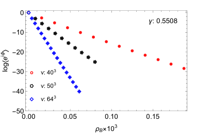
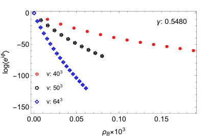
Figure 1: The logarithm of the average phase $\mathop{\rm ln}\langle\exp(i\phi)\rangle_{|\,\cdot\,|}$ as a function of the baryon density $\rho_{B}$ for different volumes at high temperature in the deconfined phase (left plot) and at low temperature in the confined phase (right plot).

In Fig. 1 we show the logarithm of the average phase $\mathop{\rm ln}\langle\exp(i\phi)\rangle_{|\,\cdot\,|}$, as obtained through eq.(71), as a function of the baryon density $\rho_{B}$, defined by $\rho_{B}=(N_{Q}/3+1/2)/L^{3}$, for different volumes and two different values of the coupling. The left plot is for the coupling $\gamma=0.5508$ for which the system is in the deconfined phase for all quark numbers, while the right plot is for $\gamma=0.5480$ for which the system is in the confined phase for all the quark numbers shown. We observe that at fixed volume the average sign goes to zero exponentially fast with the baryon density with a rate that depends on the volume.

In order to quantify further the severity of the sign problem as it scales with the volume at fixed baryon density, we define a scale parameter $L_{0}$ which parameterizes the average sign as $\exp(-V/L_{0}^{3})$ at fixed density. In Fig. 2 we show this scale parameter as a function of the baryon density for three different couplings corresponding to three different temperatures.

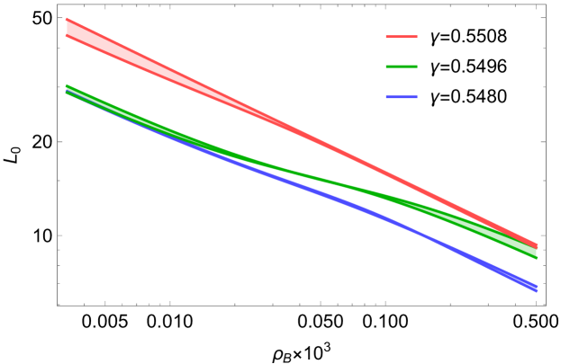
Figure 2: The scale parameter $L_{0}$ related to the severity of the sign problem as a function of the baryon density for different couplings. The lower the value of $L_{0}$, the more severe the sign problem.

The top curve corresponds to a high temperature for which the system is in the deconfined phase for all densities, while the bottom curve corresponds to a low temperature for which the system is confined for the range of density values shown. The middle curve corresponds to an intermediate temperature for which the system undergoes a first order phase transition from the confined phase at low density into the deconfined phase at higher density. This phase transition will be discussed in more detail in the next section. Here we note that $L_{0}$ decreases linearly with the density, i.e. the severity of the sign problem gets worse exponentially with increasing density, independent of whether the system is in the confined or deconfined phase. However, the scale is distinctively different in the two phases and at fixed density the sign problem in the confined phase is worse than in the deconfined phase. The behaviour is consistent with the one observed in the grand-canonical formulation (cf. Fig. 4 in [5]), but the sign problem appears to be more severe in the canonical formulation.

7 Results

From previous studies of the phase diagram in the Potts model [8, 5] one knows that the interesting physics happens at very low density which is why we concentrated our investigation of the sign problem in the previous section on that regime. We recall that the system undergoes a first order deconfinement phase transition along a critical line starting from the zero density transition point $(e^{\mu},\gamma)=(0,0.550565(10))$ down to the critical endpoint at $(e^{\mu},\gamma)=(0.000470(2),0.549463(13))$ where the system experiences a second order phase transition in the universality class of the 3-dimensional Ising model.

We first discuss our results for the quark chemical potential $\mu$, given by the partition function ratio in eq.(60), as a function of the baryon density. The function essentially provides the translation between the canonical and grand-canonical formulations. In Fig. 3 we show the results for various volumes $V=L^{3}$ at $\gamma=0.5508$ when the system is in the deconfined phase. For volumes $V\geq 25^{3}$ we observe practically no finite volume effects and we find that the chemical potential grows monotonically with increasing density. The functional dependence can be well described by an ansatz for free fermions with an effective fermion mass and we show the corresponding fit as the dashed line in Fig. 3.

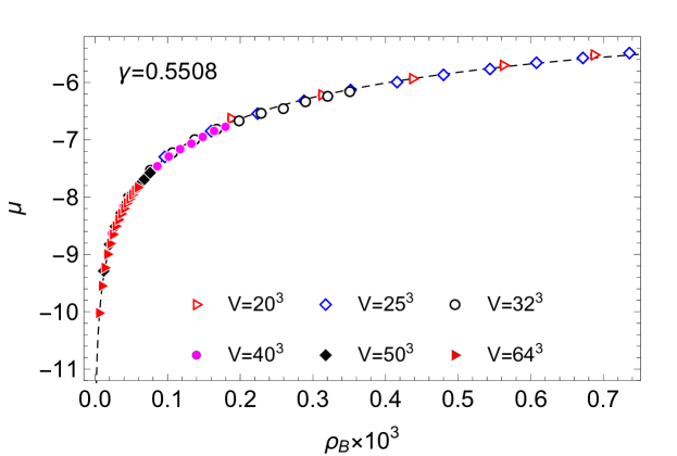
Figure 3: The quark chemical potential $\mu$ as a function of the baryon density $\rho_{B}=(N_{Q}/3+1/2)/L^{3}$ in the deconfined phase at $\gamma=0.5508$ for various volumes $V=L^{3}$. The dashed line is a phenomenological, effective description of the function in terms of the behaviour of a (free) fermion system.

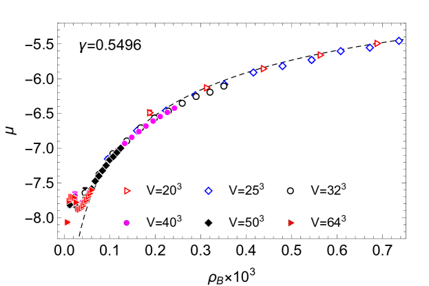
Figure 4: The quark chemical potential $\mu$ as a function of the baryon density $\rho_{B}=(N_{Q}/3+1/2)/L^{3}$ for various volumes $V=L^{3}$ at $\gamma=0.5496$, just below the zero density deconfinement transition. The dashed line is a phenomenological, effective description of the function in terms of the behaviour of a (free) fermion system.

Next, in Fig. 4 we show the results for the same quantity at $\gamma=0.5496$. At this coupling, the system at zero density is in the deconfined phase, and our data clearly shows a first order phase transition into the deconfined phase indicated by the non-monotonic behaviour of the chemical potential $\mu$ as a function of the density $\rho_{B}$. The non-monotonicity is a typical signature for a first order phase transition, and in Fig. 5 we zoom in to inspect the transition in more detail. The left plot illustrates how the behaviour is better and better resolved towards the thermodynamic limit. Since the transition happens at rather low density $\rho_{B}\lesssim 0.04\cdot 10^{-3}$ one needs at least a lattice volume of $V=40^{3}$ to see the onset of the non-monotonicity. The right plot shows the determination of the critical chemical potential corresponding to the first order phase transition on our largest volume $V=64^{3}$ using the Maxwell construction.

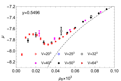
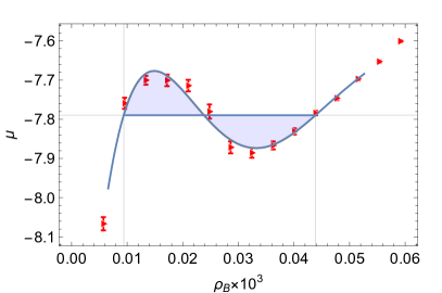
Figure 5: The quark chemical potential $\mu$ as a function of the baryon density $\rho_{B}$ at $\gamma=0.5496$ zoomed into the density region where the phase transition occurs. Left plot: Finite volume behaviour. Right plot: Maxwell construction for determining the critical chemical potential on the largest volume $V=64^{3}$.

The construction guarantees that the two shaded regions limited by the curve $\mu(\rho_{B})$ and $\mu=\mu_{c}$ (as illustrated in the plot) have the same area. The area can be related to the interface tension associated with a first order phase transition. From the Maxwell construction one can also access the values of the upper and lower densities $\rho_{\text{up,low}}$ at which the system enters or exits the coexistence phase. A systematic investigation using various interpolating functions and fit ranges yields $\mu_{c}=-7.7895(41)$ at $\gamma=0.5496$ which agrees very well with the value determined in [5]. For the upper and lower densities we obtain $\rho_{\text{up}}=0.04386(53)\cdot 10^{-3}$ and $\rho_{\text{low}}=0.00940(14)\cdot 10^{-3}$.

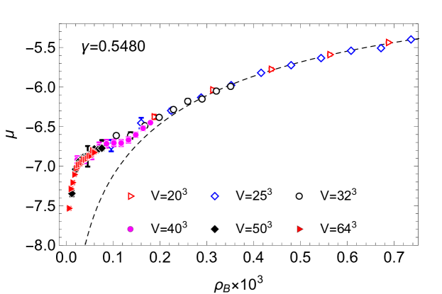
Figure 6: The quark chemical potential $\mu$ as a function of the baryon density $\rho_{B}$ at $\gamma=0.5480$ for various volumes. A smooth cross-over transition from a (confined) baryon gas behaviour at low densities into a (deconfined) fermion gas behaviour at large densities is clearly visible.

In Fig. 6 we show once more the quark chemical potential $\mu$ as a function of the baryon density for various volumes, this time at $\gamma=0.5480$ which is well below the critical endpoint. In this case, the system is in the confined phase for small baryon densities and runs smoothly into the deconfined phase at larger densities. The transition is no longer a phase transition, but rather a smooth cross-over which presents itself as a monotonic transition of the quark chemical potential from the baryonic gas form to the one describing effectively free quarks. As in the previous plots the dashed line is a phenomenological, effective description of the behaviour in terms of a free fermion gas.

Next, we investigate the quark-antiquark correlator $\langle z_{x}z_{y}^{*}\rangle_{N_{Q}=0}$ at zero density as a function of the separation $r=x-y$ for three couplings $\gamma=0.3,0.4,0.5$ in the confined phase and for one coupling $\gamma=0.6$ in the deconfined phase in Fig. 7.

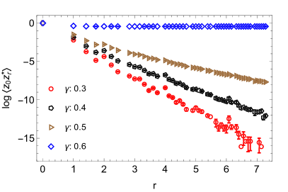
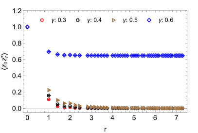
Figure 7: The quark-antiquark correlator at zero density as a function of the separation $r$ in the confined phase at $\gamma=0.3,0.4,0.5$ and in the deconfined phase at $\gamma=0.6$ on a logarithmic scale (left plot) and on a linear scale (right plot).

In the confined phase the correlator decays exponentially with the distance for large distances, with a characteristic scale that becomes longer for stronger coupling. This behaviour is consistent with the fact that at zero density the free energies of a single quark and a single antiquark are infinite because a single quark or antiquark can not exist due to Gauss’ law. This is reflected in the fact that the expectation values for a quark or an antiquark being zero, or equivalently the quark-antiquark correlator approaching zero at large distances. Above the phase transition point $\gamma=0.550565$, the correlator approaches a constant at large distances signalling deconfinement. This is illustrated in Fig. 7 by the data at $\gamma=0.6$. The finite asympotic value of the correlator at large distance indicates the spontaneous breaking of the global ${\mathbb{Z}}(3)$ symmetry and reflects the fact that the expectation values for a single quark and for a single antiquark are nonzero in the deconfined phase.

The situation is changed completely when the system is considered at nonzero baryon density. Now, the free energies for a single quark and a single antiquark are finite and the quark-quark, quark-antiquark and the antiquark-antiquark correlators are screened at large distance. This is illustrated in Fig. 8 where we show the correlators as defined in eqs.(39)-(40), as a function of the separation $r=x-y$ for a system in the confined phase at $\gamma=0.3$ (left plot) and in the deconfined phase at $\gamma=0.6$ (right plot), both in the background of 8 baryons on a $V=16^{3}$ lattice corresponding to a baryon density of $\rho_{B}\simeq 2.0\cdot 10^{-3}$. For the following discussion it is useful to think of the logarithm of the correlator as minus the potential energy (up to the factor $\gamma$).

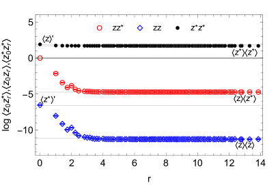
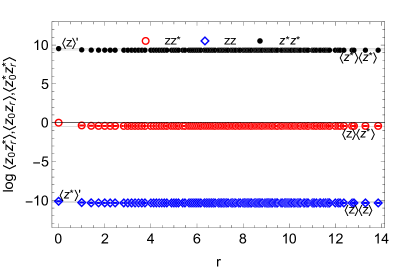
Figure 8: The (anti)quark-(anti)quark correlators as a function of the separation $r$ in the confined phase at $\gamma=0.3$ (left plot) and in the deconfined phase at $\gamma=0.6$ (right plot) in a background of 8 baryons on a $V=16^{3}$ lattice, corresponding to the density $\rho_{B}\simeq 2.0\cdot 10^{-3}$.

We first discuss the correlators in the confined phase (left plot). As before, the quark-antiquark pair at distance $r=0$ annihilates and the potential energy should therefore be zero. From eqs.(36) and (39) it is clear that in our canonical cluster formulation this is exactly realized with the improved estimator. At sufficiently large distances the expectation value is expected to factorize into the expectation values of a single quark and antiquark. The potential energy should therefore flatten out and approach the sum of the free energies of the corresponding single particles, in this case $F_{q}+F_{\bar{q}}$ obtained from $\langle z\rangle\langle z^{*}\rangle$ as indicated in the figure by the grey line. We note that our results indeed match the expectation, not only qualitatively but also quantitatively.

For the quark-quark potential energy in the background of $N_{B}$ baryons we note that two quarks at the same position are equivalent to having a single antiquark on top of an additional baryon, hence the potential energy should be equal to the free energy of a single antiquark in the corresponding background of $N_{B}+1$ baryons, obtained from $\langle z^{*}\rangle^{\prime}$. At large separation on the other hand, the correlator is expected to factorize and the potential energy is given as twice the free energy of a single quark, i.e. $2F_{q}$ obtained from $\langle z\rangle\langle z\rangle$. Similarly, two antiquarks at the same position are equivalent to a single quark on top of an antibaryon, so the potential energy is equal to the free energy of a single quark in the corresponding background with $N_{B}-1$ baryons obtained from $\langle z\rangle^{\prime}$, while at large separation it approaches twice the free energy of a single antiquark, i.e. $2F_{\bar{q}}$ as obtained from $\langle z^{*}\rangle\langle z^{*}\rangle$. In Fig. 8 these energies, respectively the logarithms of the corresponding expectation values, are again given as grey lines, and they illustrate that our results qualitatively match the expectations. The small differences we observe between the lines and the correlator data are finite volume corrections.

We further note that the asymptotes of the correlators at large distance are approximately equidistant. This is due to the fact that in each step from bottom to top, a quark is replaced by an antiquark, which approximately costs the same amount of free energy. One last feature to point out is the flatness of the antiquark-antiquark correlator as compared to the other correlators. It suggests that screening two antiquarks is almost as effective as screening a single quark in the background with one less baryon, i.e. the system in the confined phase screens antiquarks much more effective than quarks. This is of course due to the fact that the system only contains static quarks but not antiquarks as dynamical degrees of freedom.

Let us finally discuss the correlators at finite density in the deconfined phase at $\gamma=0.6$ (right plot). The discussions above for the confined phase essentially carry over without change, the only exception being that now all the correlators are very flat, i.e. they change by less than an order of magnitude over the whole range of distances. This indicates that in the deconfined phase a quark and an antiquark are screened equally efficiently, i.e. the system does no longer discriminate between a quark and an antiquark.

8 Conclusions

We have used a cluster algorithm to solve the notorious sign problem in the Potts model approximation of heavy-dense QCD, i.e. QCD with heavy quarks and large chemical potential. Our approach is based on the fact that in the canonical formulation the position of the quarks determine the triality of the clusters, i.e. the transformation properties of the weights of the clusters under ${\mathbb{Z}}(3)$ transformations. This in turn allows to identify those configurations for which the contributions to the partition function cancel exactly after averaging each cluster over its ${\mathbb{Z}}(3)$ orientations, such that only configurations remain which yield positive contributions. In this sense, the concept of cluster triality is similar to the concept of meron clusters formulated in different contexts [9] and hence the algorithm formulated here belongs to the class of meron-cluster algorithms [10, 11].

The factorization of the weights into clusters with the subsequent subaveraging of each cluster immediately yields an increase of statistics by a factor $3^{N_{C}}$ where $N_{C}$ is the number of clusters in a configuration. Since the number of clusters grows with the volume, at otherwise fixed parameters, the gain in statistics is exponential in the volume. We note that the mechanism at work here is similar to the one formulated in [12, 13] using the subset method. Here it is made to work for a three-dimensional system and away from the strong coupling limit. Furthermore, the triality properties of the clusters also allow the construction of improved estimators which receive only positive contributions. This is of course crucial for the construction of efficient simulation algorithms.

We note that the solution of the sign problem for the Potts model presented here is not the first one. In [5] the authors constructed a cluster algorithm for the Potts model at finite density in the grand-canonical formulation which solved the sign problem completely. Another approach is to use the density of states method [14]. The sign problem can also be avoided by formulating the Potts model in the flux representation [3, 4, 15, 5, 16, 17, 18]. For this reason the focus of the present paper was not so much on the physics but rather on the mechanism which forms the basis for the solution of the sign problem. In that sense the solution here can be considered as a proof of a concept which can be applied in other cases.

Various extension of our solution of the sign problem in the canonical formulation are possible. In this paper, following the spirit of [5] we have only considered positive quark occupation numbers, corresponding to a system with only quarks but no antiquarks. In the context of QCD, a more natural scenario would be to also allow for antiquarks which can form antibaryons and mesons. The triality constraints for the contributions to the partition functions and improved estimators carry over to this case without modifications. The fermion number update described in Sec. 3 and 4 becomes even simpler, because a quark-antiquark pair can be generated within a cluster using the update step in eq.(22) where the first constraint is replaced by $(1-\delta_{n_{x},-n_{\text{max}}})$. The possibility of this step enhances the efficiency of the update considerably, especially at low densities. On the other hand, the reweighting with the multiplicities as described in Sec. 5 becomes more complicated because the calculation of the multiplicities is more complex.

Applying our findings in the canonical framework to other systems at finite density is of course highly desirable. As an example we mention QCD at fixed baryon number, because this is relevant in heavy-ion collisions, and for studying few nucleon systems at low temperature. The application to QCD requires the extension of our approach to the gauge group SU(3). In this case one would apply the method only to the discrete center of the group, but it is conceivable that the discrete subset averaging is sufficient to solve or greatly ameliorate the sign problem in QCD [12, 13]. In order for this to work, one needs to embed cluster variables in continuous groups [19, 20], in particular ${\mathbb{Z}}(3)$ into SU(3) [21]. In [22] a cluster algorithm has been constructed along these lines for SU(2) on a single time slice. Extending this construction to SU(3) and combining it with the approach outlined in this paper is currently under investigation.

Appendix A Connection between the grand-canonical and the canonical partition functions

While the grand-canonical and canonical partition functions are in general equivalent and yield the same physics in the thermodynamic limit, the exact correspondence depends on the details such as the maximal fermion occupation number $n_{\text{max}}$ and the specific form of the canonical fermion weights $g[z,n]$. Here we establish the explicit relation between the canonical partition function in eq.(2), with the fermionic weights as given in eq.(3), and the corresponding grand-canonical partition function. Since the grand-canonical partition function in eq.(1) does not account for the fermionic nature of the Potts spins at large local densities, the correspondence between the grand-canonical partition function in eq.(1) and the canonical one in eq.(2) is exact only in the low-density regime where $e^{\mu}\equiv h\ll 1$, as we show below.

Using the fugacity expansion

$$Z_{\text{GC}}(h)=\sum_{N_{Q}=0}^{\infty}h^{N_{Q}}Z_{\text{C}}(N_{Q})$$ (72)

we find that the associated grand-canonical partition function is

$$\begin{split}Z_{\text{GC}}(h)=&\int{\cal D}z\,e^{-S[z]}\prod_{x}\sum_{n_{x}=0}^{n_{\text{max}}}(z_{x}h)^{n_{x}}=\int{\cal D}z\,e^{-S[z]}\prod_{x}\frac{1-(z_{x}h)^{n_{\text{max}}+1}}{1-z_{x}h}\\ =&\int{\cal D}z\,e^{-S[z]-\sum_{x}\log[1-z_{x}h]+\sum_{x}\log\left[1-(z_{x}h)^{n_{\text{max}}+1}\right]}\,.\end{split}$$ (73)

To derive the relation above we need that $h<1$ which is the case for the simulations discussed in this paper. We note that $z_{x}^{3}=1$ and $n_{\text{max}}=0\text{ mod }3$. Using the identity

$$\log[1-z_{x}f]=\frac{1}{3}\log[1-f^{3}]-z_{x}f\cdot{}_{2}F_{1}(\frac{1}{3};1;\frac{4}{3};f^{3})-\frac{1}{2}z_{x}^{*}f^{2}\cdot{}_{2}F_{1}(\frac{2}{3};1;\frac{5}{3};f^{3})\,,$$ (74)

which is valid for $|f|<1$, we find that the effective action for the grand-canonical partition function is then

$$\begin{split}S_{\text{eff}}=&S[z]+\sum_{x}z_{x}\left[h\cdot{}_{2}F_{1}(\frac{1}{3};1;\frac{4}{3};h^{3})-h^{(n_{\text{max}}+1)}h\cdot{}_{2}F_{1}(\frac{1}{3};1;\frac{4}{3};h^{3(n_{\text{max}}+1)})\right]\\ &+\sum_{x}z_{x}^{*}\frac{1}{2}\left[h^{2}\cdot{}_{2}F_{1}(\frac{2}{3};1;\frac{5}{3};h^{3})-h^{2(n_{\text{max}}+1)}h\cdot{}_{2}F_{1}(\frac{2}{3};1;\frac{5}{3};h^{3(n_{\text{max}}+1)})\right]\,.\end{split}$$ (75)

For our simulations we have $h$ of the order of $10^{-3}$ so the higher order terms, ${\cal O}(h^{2})$, contribute very little. If we keep only the first order terms our effective action simplifies to

$$S_{\text{eff}}=S[z]+h\sum_{x}z_{x}+{\cal O}(h^{2})\,.$$ (76)

This is the same action as the one in the Potts model studied by Alford et al. in [5], hence we are able to reproduce the phase diagram at low density, including the transition point at zero density $(h,\gamma)=(0,0.550565(10))$ and the critical endpoint at $(h,\gamma)=(0.000470(2),0.549463(13))$, described in Fig. 1 of that paper. Note that in [5] the parameter $\gamma$ is denoted as $\kappa$.

Appendix B Fully-dynamic connectivity problem

The Potts model in the bond formulation, as given by the partition function in eq.(13), belongs to the class of random cluster models. Simulating such systems with a local update algorithm requires one to check whether the bond under consideration is a bridge or not. A bridge bond connects two otherwise separate clusters when activated, or equivalently, breaks a cluster into two disjoint clusters when deactivated. The determination of the dynamically changing connectivity of bond clusters is a highly complex problem which in graph theory and computer science is well known under the name fully-dynamic connectivity problem. The issue here is to find data structures and algorithms with a minimal computational complexity for connectivity queries for the clusters, while dynamically adding and deleting bonds.

In the context of the Potts model [23], the problem has first been addressed by Sweeny in [24], based on the equivalence of the Potts model and the random cluster model described by Fortuin and Kasteleyn [7]. An alternative approach was suggested later by Swendsen and Wang [6] and is based on alternating updates of spin and bond variables which require only incremental connectivity information. It is well known that the Swendsen-Wang cluster construction can be dealt with efficiently with the Hoshen-Kopelman algorithm [25]. This is essentially a Find-Union algorithm acting on weighted tree data structures. Combining it with path compression to minimize the depth of the trees yields an efficient algorithm for which connectivity queries essentially have constant cost independent of the system size $L$.

Applying the same strategy to the situation of dynamically changing connectivity leads to computational critical slowing down, because whenever a bond is updated, one needs to check whether that bond acts as a bridge. Doing so requires to scan a number of bonds proportional to the typical size of the clusters. Close to the phase transition the clusters grow with the volume according to some critical exponent $\beta$ and the computational cost hence grows like ${\cal O}(L^{\beta})$ [26]. In contrast, a nearly-optimal solution for the fully-dynamic connectivity problem makes use of a spanning forest of Euler tour trees [27, 28] in order to maintain a data structure which allows for an efficient checking of the bridge property. The runtime of the corresponding algorithm only grows as ${\cal O}(\mathop{\rm ln}^{2}L)$ and we make use of it in our implementation. We note that further improvements are possible [29] yielding asymptotically to a computational complexity ${\cal O}(\mathop{\rm ln}^{2}L/\mathop{\rm ln}\mathop{\rm ln}L)$ for bond updates and ${\cal O}(\mathop{\rm ln}L/\mathop{\rm ln}\mathop{\rm ln}L)$ for connectivity queries. Additional improvements can be obtained by using randomized data structures [27]. However, one should consider that all these elaborate data structures involve some computational overhead and it is not clear a priori which of the strategies is most efficient. The fermion update in our algorithm for example only requires connectivity queries for which the Find-Union ansatz is most efficient. Finally we note that the efficiencies of some of the strategies discussed above have been investigated, and when possible compared to the one of the Swendsen-Wang algorithm, for the generic random cluster model in two dimensions in [26, 30].

Appendix C Baryon partitions

Here we describe an algorithm which generates all partitions of $N_{B}$ baryons over $N_{C}$ clusters.

procedure Partitions($N_{B}$,$N_{C}$)

     $B\leftarrow\{N_{B},0,0,\ldots\}$ $\triangleright$ $B$ is an array of $N_{C}$ entries

     loop

         Print $B$.

         Find smallest $k$ such that $B_{k}\not=0$.

         If $k=N_{C}$ exit.

         $B_{1}\leftarrow B_{k}-1$.

         If $k>1$ then $B_{k}\leftarrow 0$.

         $B_{k+1}\leftarrow B_{k+1}+1$.

     end loop

end procedure

Algorithm 1 Pseudocode to generate and print all partitions of $N_{B}$ baryons into $N_{C}$ clusters.

The logic of the algorithm is to impose an ordering relation between different partitions of $N_{B}$ into $N_{C}$ non-negative numbers, and then generate all of them by starting from the “smallest” one, $B=\{N_{B},0,\ldots,0\}$, and then successively generating the next smaller one until we get to the “largest”, $B=\{0,\ldots,0,N_{B}\}$. The order is the usual lexicographic order, that is, for two partitions $B=\{B_{1},\ldots,B_{N_{C}}\}$ and $B^{\prime}=\{B_{1}^{\prime},\ldots,B_{N_{C}}^{\prime}\}$, $B$’s order with respect to $B^{\prime}$ is determined by the order of $B_{N_{C}}$ relative to $B_{N_{C}}^{\prime}$. If $B_{N_{C}}=B_{N_{C}}^{\prime}$ then $B_{N_{C}-1}$ and $B_{N_{C}-1}^{\prime}$ are compared. This continues until we find the maximal rank $k$ where $B_{k}$ is different from $B_{k}^{\prime}$, and their order controls the order of $B$ and $B^{\prime}$. Of course $B=B^{\prime}$ if (and only if) $B_{k}=B_{k}^{\prime}$ for all $k\in\{1,\ldots,N_{C}\}$. Algorithm 1 provides the pseudocode for this procedure.

References

- [1] J. Bartholomew, D. Hochberg, P. H. Damgaard and M. Gross, Effect of Quarks on SU() Deconfinement Phase Transitions, Phys. Lett. 133B (1983) 218–220.
- [2] P. Hasenfratz, F. Karsch and I. O. Stamatescu, The SU(3) Deconfinement Phase Transition in the Presence of Quarks, Phys. Lett. 133B (1983) 221–226.
- [3] A. Patel, A Flux Tube Model of the Finite Temperature Deconfining Transition in QCD, Nucl. Phys. B243 (1984) 411–422.
- [4] T. A. DeGrand and C. E. DeTar, Phase Structure of QCD at High Temperature With Massive Quarks and Finite Quark Density: A (3) Paradigm, Nucl. Phys. B225 (1983) 590.
- [5] M. G. Alford, S. Chandrasekharan, J. Cox and U. J. Wiese, Solution of the complex action problem in the Potts model for dense QCD, Nucl. Phys. B602 (2001) 61–86, [hep-lat/0101012].
- [6] R. H. Swendsen and J.-S. Wang, Nonuniversal critical dynamics in Monte Carlo simulations, Phys. Rev. Lett. 58 (1987) 86–88.
- [7] C. M. Fortuin and P. W. Kasteleyn, On the random cluster model. 1. Introduction and relation to other models, Physica 57 (1972) 536–564.
- [8] F. Karsch and S. Stickan, The three-dimensional, three state Potts model in an external field, Phys. Lett. B488 (2000) 319–325, [hep-lat/0007019].
- [9] S. Chandrasekharan and U.-J. Wiese, Meron cluster solution of a fermion sign problem, Phys. Rev. Lett. 83 (1999) 3116–3119, [cond-mat/9902128].
- [10] S. Chandrasekharan, J. Cox, J. C. Osborn and U. J. Wiese, Meron cluster approach to systems of strongly correlated electrons, Nucl. Phys. B673 (2003) 405–436, [cond-mat/0201360].
- [11] P. Widmer, The 3-d 3-state potts model with a non-zero density of static color charges, Master’s thesis, Institute for Theoretical Physics, University of Bern, 2011.
- [12] J. Bloch, F. Bruckmann and T. Wettig, Subset method for one-dimensional QCD, JHEP 10 (2013) 140, [1307.1416].
- [13] J. Bloch and F. Bruckmann, Positivity of center subsets for QCD, Phys. Rev. D93 (2016) 014508, [1508.03522].
- [14] C. Gattringer and P. Törek, Density of states method for the spin model, Phys. Lett. B747 (2015) 545–550, [1503.04947].
- [15] J. Condella and C. E. Detar, Potts flux tube model at nonzero chemical potential, Phys. Rev. D61 (2000) 074023, [hep-lat/9910028].
- [16] S. Kim, P. de Forcrand, S. Kratochvila and T. Takaishi, The 3-state Potts model as a heavy quark finite density laboratory, PoS LAT2005 (2006) 166, [hep-lat/0510069].
- [17] Y. Delgado Mercado, H. G. Evertz and C. Gattringer, The QCD phase diagram according to the center group, Phys. Rev. Lett. 106 (2011) 222001, [1102.3096].
- [18] Y. Delgado Mercado, H. G. Evertz and C. Gattringer, Worm algorithms for the 3-state Potts model with magnetic field and chemical potential, Comput. Phys. Commun. 183 (2012) 1920–1927, [1202.4293].
- [19] F. Niedermayer, A General Cluster Updating Method for Monte Carlo Simulations, Phys. Rev. Lett. 61 (1988) 2026–2029.
- [20] F. Niedermayer, Cluster algorithms, hep-lat/9704009.
- [21] E. Onofri, Embedding Z(3) in SU(3), hep-lat/9208016.
- [22] R. Ben-Av, H. G. Evertz, M. Marcu and S. Solomon, Critical acceleration of finite temperature SU(2) gauge simulations, Phys. Rev. D44 (1991) 2953–2956.
- [23] R. B. Potts, Some generalized order-disorder transformations, Mathematical Proceedings of the Cambridge Philosophical Society 48 (1952) 106–109.
- [24] M. Sweeny, Monte Carlo study of weighted percolation clusters relevant to the Potts models, Phys. Rev. B27 (1983) 4445–4455.
- [25] J. Hoshen and R. Kopelman, Percolation and cluster distribution. 1. Cluster multiple labeling technique and critical concentration algorithm, Phys. Rev. B14 (1976) 3438–3445.
- [26] E. M. Elçi and M. Weigel, Efficient simulation of the random-cluster model, Phys. Rev. E88 (2013) 033303, [1307.6647].
- [27] M. Thorup, Near-optimal fully-dynamic graph connectivity, in Proceedings of the Thirty-second Annual ACM Symposium on Theory of Computing, STOC ’00, (New York, NY, USA), pp. 343–350, ACM, 2000. DOI:10.1145/335305.335345.
- [28] J. Holm, K. de Lichtenberg and M. Thorup, Poly-logarithmic deterministic fully-dynamic algorithms for connectivity, minimum spanning tree, 2-edge, and biconnectivity, J. ACM 48 (July, 2001) 723–760.
- [29] C. Wulff-Nilsen, Faster deterministic fully-dynamic graph connectivity, CoRR abs/1209.5608 (2012), [1209.5608].
- [30] E. M. Elçi and M. Weigel, Dynamic connectivity algorithms for Monte Carlo simulations of the random-cluster model, Journal of Physics: Conference Series 510 (2014) 012013.