Recognizing Generalized Transmission Graphs of Line Segments and Circular Sectors

Abstract

Suppose we have an arrangement $\mathcal{A}$ of $n$ geometric objects $x_{1},\dots,x_{n}\subseteq\mathbb{R}^{2}$ in the plane, with a distinguished point $p_{i}$ in each object $x_{i}$. The generalized transmission graph of $\mathcal{A}$ has vertex set $\{x_{1},\dots,x_{n}\}$ and a directed edge $x_{i}x_{j}$ if and only if $p_{j}\in x_{i}$. Generalized transmission graphs provide a generalized model of the connectivity in networks of directional antennas.

The complexity class $\exists\mathbb{R}$ contains all problems that can be reduced in polynomial time to an existential sentence of the form $\exists x_{1},\dots,x_{n}:\phi(x_{1},\dots,x_{n})$, where $x_{1},\dots,x_{n}$ range over $\mathbb{R}$ and $\phi$ is a propositional formula with signature $(+,-,\cdot,0,1)$. The class $\exists\mathbb{R}$ aims to capture the complexity of the existential theory of the reals. It lies between $\mathbf{NP}$ and $\mathbf{PSPACE}$.

Many geometric decision problems, such as recognition of disk graphs and of intersection graphs of lines, are complete for $\exists\mathbb{R}$. Continuing this line of research, we show that the recognition problem of generalized transmission graphs of line segments and of circular sectors is hard for $\exists\mathbb{R}$. As far as we know, this constitutes the first such result for a class of directed graphs.

1 Introduction

Let $\mathcal{A}$ be an arrangement of $n$ geometric objects $x_{1},\dots,x_{n}$ in the plane. The intersection graph of $\mathcal{A}$ has one vertex for each object and an undirected edge between two objects $x_{i}$ and $x_{j}$ if and only if $x_{i}$ and $x_{j}$ intersect. In particular, if the objects are (unit) disks, we speak of (unit) disk graphs. These are often used as a symmetric model for antenna reachability. In some cases, however, this symmetry is not desired, since it does not accurately model the properties of the network. For omnidirectional antennas, there is an asymmetric model called transmission graphs [2]. Transmission graphs are also defined on disks: as in disk graphs, there is one vertex per disk, and the edges indicate directed reachability. There is a directed edge between two disks if the first disk contains the center of the second disk.

Here, we present a new class of generalized transmission graphs. Now, the objects may be arbitrary sets in $\mathbb{R}^{2}$, and the points that decide about the existence of an edge can be arbitrary points in the objects.

For a given graph class, the recognition problem is as follows: given a combinatorial graph $G=(V,E)$, decide whether $G$ belongs to this class. For the recognition of geometrically defined graphs, it turned out that the complexity class $\exists\mathbb{R}$ plays a major role. The class $\exists\mathbb{R}$ was formally introduced by Schaefer [7]. It consists of all problems that are polynomial-time reducible to the set of all true sentences of the form $\exists x_{1},\dots,x_{n}:\Phi(x_{1},\dots,x_{n})$. Here, $\Phi$ is a quantifier-free formula with signature $(+,-,\cdot,0,1)$ additional to the standard boolean signature. The variables range over the reals. Hardness for this class is defined via polynomial reduction.

There are multiple classes of intersection graphs for which the recognition problem is $\exists\mathbb{R}$-complete. Kang and Müller showed this for intersection graphs of $k$-spheres [1], and Schaefer proved a similar result for intersection graphs of line segments and convex sets [7].

One prototypical $\exists\mathbb{R}$-complete problem that serves as the starting point of many reductions is Stretchability, which was among the first known $\exists\mathbb{R}$-hard problems. The original hardness-proof is due to Mnëv [6], and it was restated in terms of $\exists\mathbb{R}$ by Matoušek [5].

Here, we show that the recognition of generalized transmission graphs of line segments and of a certain type of arrangements of circular sectors is hard for $\exists\mathbb{R}$. For this, we need to extend the known proofs significantly, and we need to develop new tools to reason about geometric realizations of directed graphs. With some further work the inclusion of these problems in $\exists\mathbb{R}$ could be shown. For details see the master thesis of the first author [3].

2 Preliminaries

2.1 Graph classes

Let $x_{1},\dots,x_{n}\subseteq\mathbb{R}^{2}$ be a set of $n$ objects, and suppose that there is a distinguished point $p(x_{i})\in x_{i}$, in every object $x_{i}$. The generalized transmission graph of these objects is a directed graph $G=(V,E)$ with

$$V=\{x_{1},\dots,x_{n}\}\text{ and }E=\{(x_{i},x_{j})\mid p(x_{j})\in x_{i},1\leq i,j\leq n\}.$$

We will consider generalized transmission graphs for line segments and circular sectors. In these cases, the distinguished points $p(x_{i})$ are defined as follows: for line segments, we choose one fixed endpoint; for circular sectors, we choose the apex.

When constructing arrangements of line segments and of circular sectors below, in Sections 3 and 4, we need some notation. A line segment $\ell$ is described by an endpoint $p(\ell)$, a length $r(\ell)$, and a direction $u(\ell)$. A circular sector $c$ is presented by an apex $p(c)$, a radius $r(c)$, an opening angle $\alpha(c)$, and a direction $u(c)$. The direction is a vector in $\mathbb{R}^{2}$, and it indicates the direction of the bisector. We will call the bounding line segments the outer line segments of $c$. Let $B(c)$ be the smallest rectangle with two sides parallel to $u(c)$ that contains $c$, the bounding box of $c$.

2.2 Stretchability and combinatorial descriptions

Let $\mathcal{L}$ be an arrangement of $n$ non-vertical lines, such that no two lines in $\mathcal{L}$ are parallel. We define the combinatorial description $D(\mathcal{L})$ of $\mathcal{L}$ as follows:

Let $g$ be a vertical line that lies to the left of all intersection points of $\mathcal{L}$. We number the lines $\ell_{1},\dots,\ell_{n}$ in the order in which they intersect $g$, from top to bottom. This ordering corresponds to the ascending order of the slopes. For each line $\ell_{i}$, $i=1,\dots,n$, we have a list $O^{i}$ of the following form:

$$O^{i} =(o^{i}_{1},\dots,,o^{i}_{k}) o_{j}^{i} \subseteq\{1,\dots,,n\}$$

$$\bigcup_{j=1}^{k}o_{j}^{i} =\{1,...,n\} o_{j}^{i}\cap o_{j^{\prime}}^{i} =\emptyset,\text{ for }j\neq j^{\prime}.$$

For $i=1,\dots,n$, the order of the indices in $O^{i}$ indicates the order in which the lines $\ell_{j}$ cross $\ell_{i}$, as we travel along $\ell_{i}$ from left to right. The lists $O^{i}$, for $i=1,\dots,n$, form the combinatorial description of the arrangement $\mathcal{L}$. If $\mathcal{L}$ is simple, each $o_{j}^{i}$ is a singleton.

Given a combinatorial description $\mathcal{D}$ as above, it is relatively easy to detect whether it comes from an arrangement of pseudo-lines. This can be done by checking a few simple axioms [4]. However, the decision problem Stretchability of deciding if $\mathcal{D}$ originates from an actual arrangement of lines turns out to be significantly harder. If all sets $o_{j}^{i}$ are singletons, the same problem is called Simple-Stretchability. Both variants of the problem are complete for $\exists\mathbb{R}$ [5, 6].

3 Line segments

We now present our first result on the recognition of intersection graphs of line segments.

Theorem 3.1.

Recognizing a generalized transmission graph of line segments is $\exists\mathbb{R}$-hard.

Proof.

The proof proceeds by a reduction from Simple-Stretchability. Given an alleged description $\mathcal{D}$ of a simple arrangement of lines, we construct a graph $G_{L}=(V_{L},E_{L})$ such that $\mathcal{D}$ is realizable as a line arrangement if and only if $G_{L}$ is the generalized transmission graph of an arrangement of line segments. We set $V_{L}=A\cup B\cup C$ with

$$A =\{a_{\{i,k\}} \mid 1\leq i\neq k\leq n\},$$

$$B =\{b^{i}_{k} \mid 1\leq i\leq n,1\leq k\leq n-1\},$$

$$C =\{c_{i} \mid 1\leq i\leq n\},$$

where the $c_{i}$ are numbered in order given by $\mathcal{D}$. The $\{\ \}$ in the indices of the $a_{\{i,k\}}$ indicates that $a_{\{i,k\}}=a_{\{k,i\}}$.

Before defining the edges, we describe the intuitive meaning of the different vertices. The line segments associated with $C$ correspond to the lines $\ell_{i}$ of the arrangement. The endpoints of the line segment associated with $a_{\{i,k\}}$ will enforce that there is an intersection of the line segments for $c_{i}$ and $c_{k}$, for $1\leq i\neq k\leq n$. The endpoints of the line segments for the $b_{k}^{i}$, $k=1,\dots,n-1$, will be placed between the $a_{\{i,k\}}$ on $c_{i}$ and thus enforce the order of the intersection. When it is clear from the context, we will not explicitly distinguish between a vertex of the graph and the associated line segment. Now we define the edges:

$$E_{L} =\phantom{\cup}\{(c_{i},a_{\{i,k\}}),(c_{i},b^{i}_{k}),(b^{i}_{k},c_{i}) \mid 1\leq i\neq k\leq n\}$$

$$\phantom{=}\cup\{(b^{i}_{o^{i}_{k}},b^{i}_{o^{i}_{l}}),(b^{i}_{o^{i}_{k}},a_{\{i,o^{i}_{l}\}}) \mid 1\leq i\leq n,1\leq l<k\leq n-1\}$$

Given $\mathcal{D}$, the sets $V_{L}$ and $E_{L}$ can be constructed in polynomial time. It remains to show correctness. Suppose first that $\mathcal{D}$ is realizable, and let $\mathcal{L}=(\ell_{1},\dots,\ell_{n})$ be a simple line arrangement with $\mathcal{D}=\mathcal{D}(\mathcal{L})$. We show that there exists an arrangement $\mathcal{C}$ of line segments that realizes $G_{L}$. Let $D$ be a disk that contains all vertices of $\mathcal{L}$, with $\partial D$ having a positive distance from each vertex.

The circular order of the intersections between $\ell_{1},\dots,\ell_{n}$ and $\partial D$ is $\ell_{1},\dots,\ell_{n},\allowbreak\ell_{1},\dots,\ell_{n}$. There is no vertical line in $\mathcal{L}$, so we can add a virtual vertical line $\ell^{\prime}$ that divides the intersection points along $\partial D$ into a “left” set $D_{l}=\{q_{1}^{l},q_{2}^{l},\dots,q_{n}^{l}\}$ and a “right” set $D_{r}=\{q_{1}^{r},q_{2}^{r},\dots,q_{n}^{r}\}$ such that each set contains exactly one intersection with each line $\ell_{i}$, $i=1,\dots,n$.

For $i=1,\dots,n$, we set $c_{i}$ to $\ell_{i}\cap D$, with $p(c_{i})=q_{i}^{l}$. The $a_{\{i,k\}}$ are constructed such that $p(a_{\{i,k\}})$ is the intersection point of $\ell_{i}$ and $\ell_{k}$. The direction and length are chosen in such a way that $a_{\{i,k\}}$ intersects no other lines. Now we place the line segments $b_{o_{k}^{i}}^{i}$. They are positioned such that $p(b_{o_{k}^{i}}^{i})$ lies between $p(a_{\{i,o_{k}^{i}\}})$ and $p(a_{\{i,o_{k+1}^{i}\}})$, for $k=1,\dots,n-2$. Furthermore, we place $p(b_{o_{n-1}})$ to the right of $a_{\{i,o_{n-1}^{i}\}}$. The line segments lie on the lines $\ell_{i}$ such that $p(c_{i})$ lies in the relative interior of $b_{k}^{i}$. For an example of this construction, see Figure 1.

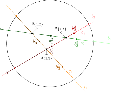
(a) Complete line segment construction for three lines

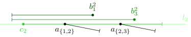
(b) Closeup of $c_{2}$. The line segments $b_{1}^{2}$ and $b_{3}^{2}$ are shifted upwards to show their positioning.

Figure 1: Construction of the line segments.

It follows from the construction that the generalized transmission graph of $\mathcal{C}$ is indeed $G_{L}$.

Now consider an arrangement $\mathcal{C}$ of line segments realizing $G_{L}$. Let $\mathcal{L}^{\prime}=(\ell_{1}^{\prime},\dots,\ell_{n}^{\prime})$ be the arrangement of lines where $\ell_{i}^{\prime}$ is the supporting line of $c_{i}$, for $i=1,\dots,n$. We claim that $\mathcal{D}=\mathcal{D}(\mathcal{L}^{\prime})$.

We first consider the role of the line segments $a_{\{i,k\}}$. Since $p(a_{\{i,k\}})$ lies on $c_{i}$ and $c_{k}$, we have $p(a_{\{i,k\}})=c_{i}\cap c_{k}$, and therefore $\ell^{\prime}_{i}$ and $\ell_{k}^{\prime}$ intersect in $p(a_{\{i,k\}})$. This ensures that all pairs of lines have an intersection point that is also the endpoint of an $a_{\{i,k\}}$. Next, we have to show that the order of the intersections along each line $\ell^{\prime}_{i}$, for $i=1,\dots,n$, is in the order as given by $\mathcal{D}$. This is guaranteed by the line segments $b^{i}_{k}$ as follows: By the definition of $E_{L}$, namely by the edges $(c_{i},b_{k}^{i})$ and $(b_{k}^{i},c_{i})$, it is ensured that all $p(b_{k}^{i})$ lie on the same line as $c_{i}$. The definition also enforces the order of the $p(a_{\{i,k\}})$ and $p(b_{k}^{i})$ along the line. Since $p(a_{\{i,o_{k}\}})$ lies on $b_{o_{k+1}}^{i}$ but not on $b_{o_{k}}^{i}$ and since all lie on the same line $c_{i}$, it has to lie between the corresponding endpoints. This enforces the correct order of the intersections. ∎

4 Circular sectors

We now consider the problem of recognizing generalized transmission graphs of circular sectors. The reduction extends the proof for Theorem 3.1, but we need to be more careful in order to enforce the correct order of intersection.

We will only consider circular sectors with opening angle $\alpha\leq\pi/4$. If $x$ and $y$ are circular sectors with $p(x)\in y$ and $p(y)\in x$, we call $x$ and $y$ a mutual couple of circular sectors. We write $\gamma(u(x),u(y))$ for the counter-clockwise angle between the vectors $u(x)$ and $u(y)$.

Observation 4.1.

Let $x$ and $y$ be a mutual couple of circular sectors, then

$$|\pi-\gamma(u(x),u(y))|\leq(\alpha(x)+\alpha(y))/2.$$

The argument is visualized in Figure 2a.

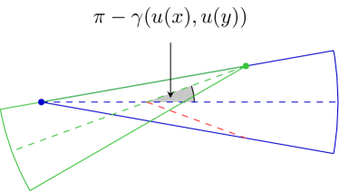
(a) Extreme position of $x$ and $y$; the symmetric case is indicated by the red line.

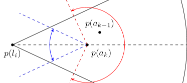
(b) $a_{k}$ and $l_{i}$ form a mutual couple, so $u(a_{k})$ lies in the blue range. The apex of $a_{k-1}$ is projected to the right of $p(a_{k})$, forcing $u(a_{k})$ to be in the red range.

Observation 4.2.

Let $x$ and $y$ be circular sectors whose bisectors intersect at an acute angle of $\beta>\max\{\alpha(x),\alpha(y)\}/2$. Then, the acute angle between the outer line segments of $x$ and the bisector of $y$ is at least $\beta-\max\left\{\alpha(x),\alpha(y)\right\}/2$.

Lemma 4.3.

Let $l$ be a circular sector and let $a_{1},\dots,a_{n}$ be circular sectors with

$$p(a_{i}) \in l, 1\leq i\leq n,$$

$$p(a_{i}) \in a_{j}, 1\leq i<j\leq n,\text{ and}$$

$$p(l) \in a_{j}, 1\leq j\leq n.$$

Then, the projection of the $p(a_{i})$ onto the directed line $\ell$ defined by $u(l)$ has the order

$$O=o_{1},\dots,o_{n}=a_{1},\dots,a_{n}.$$

Proof.

Each $a_{i}$ forms a mutual couple with $l$. Thus, with Observation 4.1, we get

$$|\pi-\gamma\left(u(a_{i}),u(l)\right)| \leq\pi/4.$$ (1)

Assume that the order of the projection differs from $O$. Let $O^{\prime}=o^{\prime}_{1},\dots,o^{\prime}_{n}$ be the actual order of the projection of the $p(a_{i})$ onto $\ell$. Let $j$ be the first index with $o_{j}^{\prime}\neq o_{j}$ and $o^{\prime}_{j}=a_{k}$. Then, there is an $o^{\prime}_{i}$, $i>j$, with $o^{\prime}_{i}=a_{k-1}$. By definition, $p(a_{k-1})$ has to be included in $a_{k}$, while still being projected on $\ell$ to the right of $p_{k}$. This is only possible if

$$|\pi-\gamma(u(a_{j}),\ell)|>\frac{\pi}{2}-\frac{\alpha(a_{k})}{2}\geq\frac{\pi}{2}-\frac{\pi}{8}=\frac{3\pi}{8}>\frac{\pi}{4}$$

This is a contradiction to (1), and consequently the order of the projection is as claimed. The possible ranges of the angles are illustrated in Figure 2b. ∎

An arrangement $\mathcal{C}$ of circular sectors is called equiangular if $\alpha(c)=\alpha(c^{\prime})$ for all circular sectors $c,c^{\prime}\in\mathcal{C}$.

Let $c,c^{\prime}$ be two circular sectors of $\mathcal{C}$, and assume that $d\in\mathcal{C}$ is a circular sector with $p(d)\in c$ and $p(d)\in c^{\prime}$, such that $c$ and $c^{\prime}$ do not form both a mutual couple with the same circular sector. Moreover let $\beta_{\text{min}}$ be the smallest acute angle between the bisector of any pair $c,c^{\prime}$ with this property. We will call the arrangement wide spread if

$$\beta_{\text{min}}\geq 2\cdot\max_{c\in\mathcal{C}}(\alpha(c))$$

The possible situations are depicted in Figure 2.

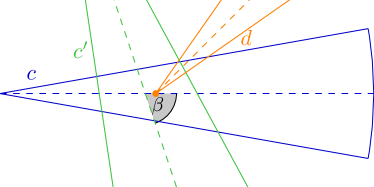
(c) Constraint on the angle.

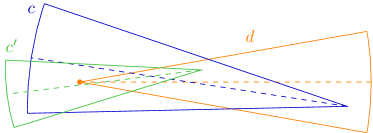
(d) No constraint on the angle.

Figure 2: The wide spread condition.

Definition 4.4.

The recognition problem of the generalized transmission graphs of equiangular, wide spread circular sectors is called Sector.

Now we want to show that Sector is hard for $\exists\mathbb{R}$. This is done in three steps. First, we give a polynomial-time construction that creates an arrangement of circular sectors from an alleged combinatorial description of a line arrangement. Then we show that this construction is indeed a reduction and therefore show the $\exists\mathbb{R}$-hardness of Sector.

Construction 4.5.

Given a description $\mathcal{D}$ where all $o_{i}$ are singletons, we construct a graph $G_{L}=(V_{L},E_{L})$. For this construction, let $1\leq i,k,l\leq n$, $1\leq m,m^{\prime},m^{\prime\prime}\leq 3$. The set of vertices is defined as follows:

$$V_{L} =\phantom{\cup}\{c_{im}\}\cup\{a^{im}_{km^{\prime}} \mid i\neq k\}\cup\{b^{im}_{km^{\prime}} \mid i\neq k\}$$

As for the line segments, we do not distinguish between the vertices and the circular sectors. For the vertices $a_{km^{\prime}}^{im}$ and $b_{km^{\prime}}^{im}$, the upper index indicates the $c_{im}$ with whom $a_{km^{\prime}}^{im}$ and $b_{km^{\prime}}^{im}$ form a mutual couple. The lower index hints at a relation to $c_{km^{\prime}}$. In most cases, the upper index is $im$ and the lower index differs. For better readability, the indices are marked bold ($a_{\mathbf{im}}^{\mathbf{km^{\prime}}}$), if $im$ is the lower index.

The bisectors of the circular sectors $c_{i2}$ will later define the lines of the arrangement. The circular sectors $a^{im}_{km^{\prime}}$ and $a_{\mathbf{im}}^{\mathbf{km^{\prime}}}$ have a similar role as the $a_{\{i,k\}}$ in the construction for the line segments. They enforce the intersection of $c_{im}$ and $c_{km^{\prime}}$. Similar to the $b_{k}^{i}$, the $b_{km^{\prime}}^{im}$ help enforcing the intersection order.

We describe $E_{L}$ on a high level. For a detailed technical description, refer to Section A.1. We divide the edges of the graph into categories. The first category, $E_{I}$, contains the edges that enforce an intersection between two circular sectors $c_{im}$ and $c_{km^{\prime}}$, for $k<l$. The edges of the next category $E_{C}$ enforce that each $a_{km^{\prime}}^{im}$ and each $b_{km^{\prime}}^{im}$ forms a mutual couple with $c_{im}$.

$$\begin{aligned} E_{I}=\phantom{\cup}&\{(c_{im},a_{km^{\prime}}^{im})&&\mid i\neq k\}\\ \phantom{=}\cup&\{(c_{im},a^{km^{\prime}}_{im})&&\mid i\neq k\}\end{aligned} \begin{aligned} E_{C}=\phantom{\cup}&\{(a_{km^{\prime}}^{im},c_{im})&&\mid i\neq k\}\\ \phantom{=}\cup&\{(c_{im},b_{km^{\prime}}^{im})&&\mid i\neq k\}\\ \phantom{=}\cup&\{(b_{km^{\prime}}^{im},c_{im})&&\mid i\neq k\}\end{aligned}$$

The edges in the next categories enforce the local order. The first category, called $E_{\text{GO}}$, enforces a global order in the sense that the apexes of all $a_{{o_{j}}m^{\prime}}^{im}$ and $b_{{o_{j}}m^{\prime}}^{im}$ will be projected to the left of any $a_{{o_{k}}m^{\prime}}^{im}$ and $b_{{o_{k}}m^{\prime}}^{im}$ with $k>j$. Additionally, all $a_{\mathbf{im}}^{\mathbf{o_{j}m^{\prime}}}$ will be included in $a_{{o_{k}}m^{\prime}}^{im}$ and $b_{{o_{k}}m^{\prime}}^{im}$. The projection order is enforced by the construction described in Lemma 4.3, the inclusion is enforced by adding the appropriate edges.

It remains to consider the local order of the six circular sectors ($a_{j1}^{im},\dots,a_{j3}^{im},\allowbreak b_{j1}^{im},\dots,b_{j3}^{im}$) that are associated with $c_{im}$ for each intersecting circular sector $c_{j2}$. The projection order of these is either “$1$, $2$, $3$” or “$3$, $2$, $1$”, depending on the order of $l_{i}$ and $l_{j}$ on the vertical line. If $l_{j}$ is below $l_{i}$, the order on $c_{im}$ is “$1$, $2$, $3$”; in the other case, it is “$3$, $2$, $1$”. This is again enforced by adding the edges as defined in Lemma 4.3. For a possible realization of this graph, see Figures 3 and 4. This construction can be carried out in polynomial time.

Now we show that Construction 4.5 gives us indeed a reduction:

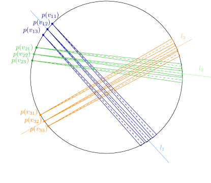
Figure 3: Construction of the circular sectors $c_{im}$ based on a given line arrangement

Lemma 4.6.

Suppose there is a line arrangement $\mathcal{L}=\{\ell_{1},\dots,\ell_{n}\}$ realizing $\mathcal{D}$, then there is an equiangular, wide spread arrangement $\mathcal{C}$ of circular sectors realizing $G_{L}$ as defined in Construction 4.5.

Proof.

We construct the containing disk $D$, and the sets of intersection points $D_{l}$ and $D_{r}$ as in the proof of Theorem 3.1. By $\ell_{im}$, we denote the directed line through the bisector of the circular sector $c_{im}$. Let $\alpha_{\text{min}}$ be the smallest acute angle between any two lines of $\mathcal{L}$. The angle $\alpha$ for $\mathcal{C}$ will be set depending on $\alpha_{\text{min}}$ and the placement of the constructed circular sectors $c_{im}$.

In the first step, we place the circular sectors $c_{i2}$. They are constructed such that their apexes are on $q_{i}^{l}$ and their bisectors are exactly the line segments $\ell_{i}\cap D$. We place $p(c_{i1})$ in clockwise direction next to $p(c_{i2})$ onto the boundary of $D$. The distance between $p(c_{i1})$ and $p(c_{i2})$ on $\partial D$ is some small $\tau>0$. The point $p(c_{i3})$ is placed in the same way, but in counter-clockwise direction from $p(c_{i2})$. The bisectors of all $c_{im}$ are parallel. The radii for $c_{i1}$ and $c_{i3}$ are chosen to be the length of the line segments $\ell_{i1}\cap D$ and $\ell_{i3}\cap D$.

The distance $\tau$ must be small enough so that no intersection of any two original lines lies between $\ell_{i1}$ and $\ell_{i3}$. Let $\beta$ be the largest angle such that if the angle of all $c_{im}$ is set to $\beta$, there is always at least one point in $c_{im}$ between the bounding boxes $B$ of two circular sectors with consecutively intersecting bisectors. Since $\mathcal{L}$ is a simple line arrangement, this is always possible. The angle $\alpha$ for the construction is now set to $\min\left\{\alpha_{\text{min}}/2,\beta\right\}$. This first part of the construction is illustrated in Figure 3.

Now we place the remaining circular sectors. Their placement can be seen in Figure 4. The points $p(a_{km^{\prime}}^{im})$ all lie on $\ell_{im}$ with a distance of $\delta$ to the left of the intersection of $\ell_{im}$ and $\ell_{km^{\prime}}$. By “to the left”, we mean that the point lies closer to $p(c_{im})$ on the line $\ell_{im}$ than the intersection point. The distance $\delta$ is chosen small enough such that $p(a_{km^{\prime}}^{im})$ lies inside of all $a_{\mathbf{im}}^{\mathbf{km^{\prime}}}$ that have a larger distance to $p(c_{\mathbf{km^{\prime}}})$ than $p(a_{km^{\prime}}^{im})$. The direction of the circular sector $a_{km^{\prime}}^{im}$ is set to $-u(c_{im})$, and its radius is set to $r(a_{o_{k}m^{\prime}}^{im})=\operatorname{dist}(p(a_{km^{\prime}}^{im}),p(c_{im}))+\varepsilon$, for $\varepsilon>0$. This lets $p(c_{im})$ lie on the bisecting line segment of every circular sector $a_{km^{\prime}}^{im}$. The directions and radii for the $b_{km^{\prime}}^{im}$ are chosen in the same way as for the $a_{km^{\prime}}^{im}$. The apexes of $b_{km^{\prime}}^{im}$ are placed such that they lie between the corresponding bounding boxes $B(c_{km^{\prime}})$. For $\alpha$ small enough, this is always possible.

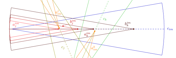
Figure 4: Detailed construction inside of one circular sector $c_{im}$.

It follows directly from the construction that the generalized transmission graph of this arrangement is $G_{L}$. A detailed argument can be found in Section A.2. ∎

Lemma 4.7.

Suppose there is an equiangular, wide spread arrangement $\mathcal{C}$ of circular sectors realizing $G_{L}$ as defined in Construction 4.5, then there is an arrangement of lines realizing $\mathcal{D}$.

Proof.

From $\mathcal{C}$, we construct an arrangement $\mathcal{L}=(\ell_{1},\dots,\ell_{n})$ of lines such that $\mathcal{D}(\mathcal{L})=\mathcal{D}$ by setting $\ell_{i}$ to the line spanned by $u(c_{i2})$. Now, we show that this line arrangement indeed satisfies the description, e.g., that the intersection order of the lines is as indicated by the description.

All $a_{km^{\prime}}^{im}$ and $b_{km^{\prime}}^{im}$ form mutual couples with $c_{im}$. Thus, Lemma 4.3 can be applied to them. It follows that the order of the projections of the apexes of the circular sectors is known. In particular, the order of projections of the $p(a_{j2}^{i2})$ onto $\ell_{i}$ is the order given by $\mathcal{D}$ and $p(b_{o_{j}2}^{i2})$ is projected between $p(a_{o_{j}2}^{i2})$ and $p(a_{o_{j+1}2}^{i2})$.

Now, we have to show that the order of intersections of the lines corresponds to the order of the projections of the $p(a_{j2}^{i2})$. This will be done through a contradiction. We consider two circular sectors $c_{j2}$ and $c_{k2}$. Assume that the order of the projection of the apexes of $a_{j2}^{i2}$ and $a_{k2}^{i2}$ onto $\ell_{i}$ is $p(a_{j2}^{i2})$, $p(a_{k2}^{i2})$, while the order of intersection of the lines is $\ell_{k}$, $\ell_{j}$.

Note that by the definition of the edges of $G_{L}$, $c_{j2}$ and $c_{k2}$ share the apexes of $a_{j2}^{k2}$ and $a_{k2}^{j2}$, but there is no circular sector they both form a mutual couple with and thus the angle between their bisecting line segments is large.

There are two main cases to consider, based on the position of the intersection point $p$ of $\ell_{j}$ and $\ell_{k}$ relative to $c_{i2}$:

Case one $p\notin c_{i2}$:

If $p$ does not lie in $c_{i2}$, then $\ell_{j}$ and $\ell_{k}$ divide $c_{i2}$ into three parts. Let $s_{j},s_{k}$ be the outer line segments of $c_{j2}$ and $c_{k2}$ that lie in the middle part of this decomposition. A schematic of this situation can be seen in Figure 5a.

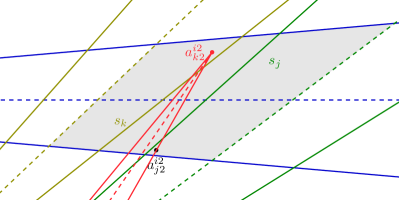
(a) Case one, $a_{k2}^{i2}$ cannot reach $a_{j2}^{i2}$.

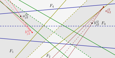
(b) Case two, $b_{j2}^{i2}$ cannot lie in $F_{1}$ or $F_{3}$.

From Observation 4.2 and since $\mathcal{C}$ is an equiangular, wide spread arrangement it follows that $|\pi-\gamma(s_{j},u(c_{i}))|>3\alpha/2\text{ and }|\pi-\gamma(s_{k},u(c_{i}))|>3\alpha/2$.

In order to have an intersection order that differs from the projection order, the circular sector $a_{k2}^{i2}$ has to reach $p(a_{j2}^{i2})$. The latter point is projected to the left of $a_{k2}^{i2}$ but lies right of $s_{k}$. The directed line segment $d$ from $p(a_{k2}^{i2})$ to $p(a_{k2}^{j2})$ has to intersect $s_{j}$ and $s_{k}$, and thus it has to hold that $|\pi-\gamma(d,u(c_{i2}))|\geq 3\alpha/2$. The line segment $d$ has to lie inside of $a_{k2}^{i2}$, which is only possible if $|\pi-\gamma(u(a_{k2}^{i2}),u(c_{i}))|>\alpha$. However, this is a contradiction to $|\pi-\gamma(u(a_{k}^{i}),u(c_{i}))|\leq\alpha$, which follows from Observation 4.1.

Case two $p\in c_{i2}$:

W.l.o.g., let $u(c_{i2})=\lambda\cdot(1,0)$, $\lambda>0$, and let $\mathcal{F}=\{F_{1},F_{2},F_{3},F_{4}\}$ be the decomposition of the plane into faces induced by $\ell_{j}$ and $\ell_{k}$. Here, $F_{1}$ is the face with $p(c_{i2})$, and the faces are numbered in counter-clockwise order.

We consider the possible placements of $p(b_{j2}^{i2})$ in one of the face. First, we show that $p(b_{j2}^{i2})$ cannot lie in $F_{1}$ or in $F_{3}$. From the form of $E_{\text{GO}}$, we know that $p(a_{j2}^{i2})$ has to be projected left of $p(b_{j2}^{i2})$ and $p(a_{j2}^{i2})$ has to lie inside of $b_{j2}^{i2}$; see Figure 5b for a schematic of the situation. If $p(b_{j2}^{i2})$ lies in $F_{1}$, the line segment in $b_{j2}^{i2}$ that connects $p(b_{j2}^{i2})$ and $p(a_{j2}^{i2})$ has to cross an outer line segment of $c_{j2}$. This yields the same contradiction as in the first case. If $p(b_{j2}^{i2})$ were in $F_{3}$, an analogous argument holds for $p(b_{j2}^{i2})$, which has to lie inside of $a_{k2}^{i2}$.

This leaves $F_{2}$ and $F_{4}$ as possible positions for $b_{j2}^{i2}$. W.l.o.g., let $b_{j2}^{i2}$ be located in $F_{4}$. We divide $c_{j2}$ and $c_{k2}$ by $\ell_{k}$ or $\ell_{j}$, respectively, into two parts, and denote the parts containing the line segments that are incident to $F_{4}$ by $J$ and $K$. Then, again by using that the arrangement is wide spread, it can be seen that $p(a_{j2}^{i2})$ and $p(a_{k2}^{i2})$ are located in $J$ and $K$. The possible placement is visualized in Figure 5c.

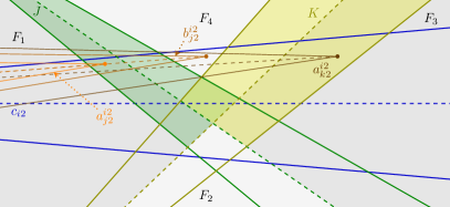
(c) The localization of $a_{j2}^{i2}$ and $a_{k2}^{i2}$.

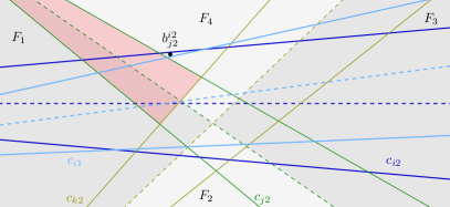
(d) $p$ can not lie in $c_{i1}$.

The argument so far yields that if $p\in c_{i2}$, then the intersection order of $\ell_{j}$ and $\ell_{k}$ with $\ell_{i}$ is the same as the order of projection if $\ell_{i}$ lies above $p$, and is the inverse order if $\ell_{i}$ lies below $p$. The uncertainty of this situation is not desirable. By considering the circular sectors $c_{i1}$ and $c_{i3}$, we will now show that such a situation cannot occur.

First, we show that $c_{i1}$ and $c_{i3}$ cannot contain the intersection point of $\ell_{j}$ and $\ell_{k}$. W.l.o.g., assume that the intersection point lies in $c_{i1}$. Then, $b_{j2}^{i1}$ is included in either $F_{2}$ or $F_{4}$. Consider the case that $b_{j2}^{i1}$ lies in $F_{4}$. Since $u(c_{i2})=\lambda\cdot(1,0)$ and since one of the outer line segments of $c_{i2}$ has to lie beneath $p$, there is only one outer line segment of $c_{i2}$ that intersects $F_{4}\setminus(J\cup K)$, $J$ and $K$. There are at most two intersection points of this outer line segment with $\partial c_{i1}$. This implies that there is no intersection point of $\partial c_{i2}$ and $\partial c_{i1}$ in at least one of $J$, $K$, and $F_{4}\setminus(J\cup K)$. If there is no intersection point, then $c_{i1}$ and $c_{i2}$ overlap in this interval. W.l.o.g., let this area be $J$, and let $c_{i1}\cap J$ be fully contained in $c_{i2}\cap J$. Then, $p(a_{j1}^{im})$ cannot be placed. Consequently, this situation is not possible. The argument is depicted in Figure 5d.

If $p(b_{j2}^{i1})$ was included in $F_{2}$, then the order of projection of $p(a_{k2}^{i2})$ and $p(a_{j2}^{i2})$ would be the same order as the order of intersections of $\ell_{j}$ and $\ell_{k}$ with a parallel line to $\ell_{i}$ that lies below $\ell_{i}$. This order is the inverse order of the order of projection in $c_{i2}$. Since the order of the projection as defined by $E_{\text{GO}}$ depends only on $k$ and $i$, the order of projection of $p(a_{j2}^{im})$ and $p(a_{k2}^{im})$ has to be the same in all $c_{im}$. This implies that $p(b_{k2}^{i1})$ is not included in $F_{2}$.

Now, we know that $c_{i1}$ and $c_{i3}$ do not contain the intersection point. This implies that the argument from the case $p\notin c_{i2}$ can be applied to them and the order of intersection in $c_{i1}$ and $c_{i3}$ is the same as the order of the projections of $p(a_{j2}^{i1})$ and $p(a_{k2}^{i1})$. This order is the same in all three $c_{im}$, and thus the bisectors of $c_{i1}$ and $c_{i3}$ have to lie on the same side of the intersection point. Furthermore, the points $p(a_{j2}^{i1})$ and $p(a_{j2}^{i3})$ have to lie in $J$ but outside of $c_{i2}$. This implies that $\ell_{i1}$ and $\ell_{i3}$ both intersect $\ell_{j}$ and $\ell_{k}$ either before $\ell_{i}$ or after $\ell_{i}$, while $p(b_{j2}^{i2})$ lies in $F_{4}$.

The edges for the local order define that the order of projection onto $\ell_{j}$ is $p(a_{j2}^{i1})$, $p(a_{j2}^{i2})$, $p(a_{j2}^{i3})$ (or the reverse), and the analogous statement holds for $\ell_{k}$. This order is not possible with $c_{i1}$ and $c_{i3}$, both lying above or below $c_{i2}$, which implies that the intersection point cannot lie in $c_{i2}$. Since the order of intersection is the same as the order of the projection, if $p\notin c_{i2}$ and a situation with $p\in c_{i2}$ is not possible, we have shown that $\mathcal{D}(\mathcal{L})=\mathcal{D}$. ∎

With the tools from above, we can now give the proof of the main result of this section:

Theorem 4.8.

Sector is hard for $\exists\mathbb{R}$.

Proof.

The theorem follows from Constructions 4.5, 4.6 and 4.7. ∎

5 Conclusion

We have defined the new graph class of generalized transmission graphs as a model for directed antennas with arbitrary shapes. We showed that the recognition of generalized transmission graphs of line segments and a special form of circular sectors is $\exists\mathbb{R}$-hard.

For the case of circular sectors, we needed to impose certain conditions on the underlying arrangements. The wide spread condition in particular seems to be rather restrictive. We assume that this condition can be weakened, if not dropped, while the problem remains $\exists\mathbb{R}$-hard.

Ours are the first $\exists\mathbb{R}$-hardness results on directed graphs that we are aware of. We believe that this work could serve as a starting point for a broader investigation into the recognition problem for geometrically defined directed graph models, and to understand further what makes these problems hard.

Acknowledgments. We would like to thank an anonymous reviewer for pointing out a mistake in Observation 4.1.

Appendix A Missing proofs and constructions

A.1 Full construction for SECTOR

Let the vertices of the construction be defined as in Construction 4.5. We divide the edges of the graph into categories. The first category $E_{I}$ contains the edges that enforce an intersection of two circular sectors $c_{im}$ and $c_{km^{\prime}}$ for $k<l$.

$$E_{I}=\Big{\{}\big{(}c_{im},a_{km^{\prime}}^{im}\big{)},\big{(}c_{im},a^{km^{\prime}}_{im}\big{)}\,\Big{|}\,i\neq k\Big{\}}.$$

The edges $E_{C}$ enforce that each $a_{km^{\prime}}^{im}$ and each $b_{km^{\prime}}^{im}$ forms a mutual couple with $c_{im}$.

$$E_{C}=\Big{\{}\big{(}a_{km^{\prime}}^{im},c_{im}\big{)},\big{(}c_{im},b_{km^{\prime}}^{im}\big{)},\big{(}b_{km^{\prime}}^{im},c_{im}\big{)}\,\Big{|}\,i\neq k\Big{\}}.$$

The edges of $E_{\text{GO}}$ will enforce the order of the projection of the apexes of $a_{o_{k}m^{\prime}}^{im}$, $a_{o_{l}m^{\prime\prime}}^{im}$, $b_{o_{k}m^{\prime}}^{im}$, and $b_{o_{l}m^{\prime\prime}}^{im}$ for $k>l$ onto the bisector of $c_{im}$. They are chosen such that $p(a_{o_{k}m^{\prime}}^{im})$ will be projected closer to $p(c_{im})$ than $p(a_{o_{l}m^{\prime\prime}}^{im})$, for $k<l$. Also included in $E_{\text{GO}}$ are edges that enforce that all $p(a_{\mathbf{im}}^{\mathbf{o_{k}m^{\prime}}})$ are included in the circular sectors $a_{o_{l}m^{\prime\prime}}^{im}$ and $b_{o_{l}m^{\prime\prime}}^{im}$.

$$E_{\text{GO}} =\phantom{\cup}\Big{\{}(a_{o_{k}m^{\prime}}^{im},a_{o_{l}m^{\prime\prime}}^{im}),(a_{o_{k}m^{\prime}}^{im},a^{\mathbf{o_{l}m^{\prime\prime}}}_{\mathbf{im}}),(a_{o_{k}m^{\prime}}^{im},b_{o_{l}m^{\prime\prime}}^{im}),$$

$$\phantom{=\cup\Big{\{}}(b_{o_{k}m^{\prime}}^{im},a_{o_{l}m^{\prime\prime}}^{im}),(b_{o_{k}m^{\prime}}^{im},a^{\mathbf{o_{l}m^{\prime\prime}}}_{\mathbf{im}}) \Big{|}\,i\neq k,k>l\Big{\}}.$$

The last two categories of edges will enforce the projection order of the apexes of $a_{o_{k}1}^{im}$, $a_{o_{k}2}^{im}$, $a_{o_{k}3}^{im}$, and $b_{o_{k}1}^{im}$, $b_{o_{k}2}^{im}$, $b_{o_{k}3}^{im}$ onto the bisector of $c_{im}$. This order is $a_{o_{k}1}^{im}$, $b_{o_{k}1}^{im}$, $a_{o_{k}2}^{im}$, $b_{o_{k}2}^{im}$, $a_{o_{k}3}^{im}$ $b_{o_{k}3}^{im}$, if $o_{k}>i$, and the inverse order, otherwise. The edges for the first case are $E_{\text{LOI}}$, and the edges for the second case are $E_{\text{LOD}}$. We set

$$E_{\text{LOI}} =\phantom{\cup}\Big{\{}(a_{o_{k}m^{\prime}}^{im},a_{o_{k}m^{\prime\prime}}^{im}),(a_{o_{k}m^{\prime}}^{im},a^{\mathbf{o_{k}m^{\prime\prime}}}_{\mathbf{im}}),$$

$$\phantom{=\cup\Big{\{}}(a_{o_{k}m^{\prime}}^{im},b_{o_{k}m^{\prime\prime}}^{im}),(b_{o_{k}m^{\prime}}^{im},b_{o_{k}m^{\prime\prime}}^{im}) \Big{|}\,i\neq k,m^{\prime\prime}<m^{\prime},o_{k}>i\Big{\}}$$

$$\phantom{=}\cup\Big{\{}(b_{o_{k}m^{\prime}}^{im},a_{o_{k}m^{\prime\prime}}^{im}),(b_{o_{k}m^{\prime}}^{im},a^{\mathbf{o_{k}m^{\prime\prime}}}_{\mathbf{im}}) \Big{|}\,i\neq k,m^{\prime\prime}\leq m^{\prime},o_{k}>i\Big{\}}$$

and

$$E_{\text{LOD}} =\phantom{\cup}\Big{\{}(a_{o_{k}m^{\prime}}^{im},a_{o_{k}m^{\prime\prime}}^{im}),(a_{o_{k}m^{\prime}}^{im},a^{\mathbf{o_{k}m^{\prime\prime}}}_{\mathbf{im}}),$$

$$\phantom{=\cup\Big{\{}}(a_{o_{k}m^{\prime}}^{im},b_{o_{k}m^{\prime\prime}}^{im}),(b_{o_{k}m^{\prime}}^{im},b_{o_{k}m^{\prime\prime}}^{im}) \Big{|}\,i\neq k,m^{\prime\prime}>m^{\prime},o_{k}<i\Big{\}}$$

$$\phantom{=}\cup\Big{\{}(b_{o_{k}m^{\prime}}^{im},a_{o_{k}m^{\prime\prime}}^{im}),(b_{o_{k}m^{\prime}}^{im},a^{\mathbf{o_{k}m^{\prime\prime}}}_{\mathbf{im}}) \Big{|}\,i\neq k,m^{\prime\prime}\geq m^{\prime},o_{k}<i\Big{\}}.$$

The set of all edges is defined as

$$E_{L}=E_{I}\cup E_{C}\cup E_{\text{GO}}\cup E_{\text{LOI}}\cup E_{\text{LOD}}.$$

A.2 Remaining proof for Lemma 4.6

Lemma A.1.

The generalized transmission graph of the arrangement $\mathcal{C}$ of circular sectors constructed in Lemma 4.6 is $G_{L}$

Proof.

As $\delta$ is chosen small enough that $a_{km^{\prime}}^{im}$ and $a_{\mathbf{im}}^{\mathbf{km^{\prime}}}$ lie in $c_{im}$, the edges of $E_{I}$ are created. Since $b_{km^{\prime}}^{im}$ and $a_{km^{\prime}}^{im}$ have the inverse direction of $c_{im}$ and the radii are large enough, $p(c_{im})$ is included in $a_{km^{\prime}}^{im}$ and in $b_{km^{\prime}}^{im}$. Hence all edges in $E_{C}$ are created.

By the choice of the radii and the direction, $a_{o_{k}m^{\prime}}^{im}$ includes all apexes of circular sectors that lie on $\ell_{im}$ and closer to $p(c_{m})$ than $p(a_{o_{k}m^{\prime}}^{im})$. Furthermore, $\delta$ is small enough such that all $a_{\mathbf{im}}^{\mathbf{o_{l}m}^{\prime\prime}}$, $l<k$, are included in $a_{o_{k}m^{\prime}}^{im}$. This implies that edges from $E_{\text{GO}}$ are present in the generalized transmission graph of $\mathcal{C}$.

The only edges that have not been considered yet are the edges in $E_{\text{LOI}}$ and $E_{\text{LOD}}$. For a circular sector $a_{o_{k}m^{\prime}}^{im}$ with $o_{k}>i$, the slope of $\ell_{o_{k}}$ is larger than the slope of $\ell_{i}$. By the counter-clockwise construction, $\ell_{o_{k}1}$ lies above $\ell_{o_{k}2}$. This implies that the intersection point of $\ell_{o_{k}1}$ and $\ell_{im}$ lies closer to $p(c_{im})$ than the intersection points with $\ell_{o_{k}2}$ or $\ell_{o_{k}3}$. The presence of the edges can now be seen by the same argument as for the edges of $E_{\text{GO}}$. Symmetrical considerations can be made for the edges of $E_{\text{LOD}}$.

It remains to show that no additional edges are created. Note that all apexes of the circular sectors lie inside of $D$ and that all $a_{km^{\prime}}^{im}\cap D$ and $b_{km^{\prime}}^{im}\cap D$ are included in the boxes $B(c_{im})$.

Since only the apexes of $a_{km^{\prime}}^{im}$, $a_{\mathbf{im}}^{\mathbf{km^{\prime}}}$, and $b_{km^{\prime}}^{im}$ lie in $c_{im}$, there are no additional edges starting at $c_{im}$. The rectangles $B(c_{im})$ are disjoint on the boundary of $D$ and all $a_{km^{\prime}}^{im}\cap D$ and $b_{km^{\prime}}^{im}\cap D$ lie inside of $B(c_{im})$. This implies that there are no additional edges ending at $c_{im}$. Now, we have to consider additional edges starting at $a_{km^{\prime}}^{im}$ and $b_{km^{\prime}}^{im}$. Note that $\alpha\leq\pi/4$ enforces that no circular sector $a_{km^{\prime}}^{im}$ or $b_{km^{\prime}}^{im}$ can reach an apex having a larger distance to $p(c_{im})$. Also, note that there are edges for all circular sectors with smaller distances in $E_{\text{GO}}$, $E_{\text{LOD}}$ or $E_{\text{LOI}}$. This covers all possible additional edges. ∎

References

- [1] R. J. Kang and T. Müller. Sphere and dot product representations of graphs. Discrete Comput. Geom., 47(3):548–568, 2012.
- [2] H. Kaplan, W. Mulzer, L. Roditty, and P. Seiferth. Spanners and reachability oracles for directed transmission graphs. In Proc. 34th Int. Sympos. Comput. Geom. (SoCG), pages 156–170, 2015.
- [3] K. Klost. Complexity of recognizing generalized transmission graphs, March 2017.
- [4] D. E. Knuth. Axioms and Hulls, volume 606 of Lecture Notes in Computer Science. Springer-Verlag, 1992.
- [5] J. Matoušek. Intersection graphs of segments and . arXiv:1406.2636, 2014.
- [6] N. E. Mnëv. Realizability of combinatorial types of convex polyhedra over fields. Journal of Soviet Mathematics, 28(4):606–609, 1985.
- [7] M. Schaefer. Complexity of some geometric and topological problems. In Proc. 17th Int. Symp. Graph Drawing (GD), pages 334–344, 2009.