i-process contribution of rapidly accreting white dwarfs to
the solar composition of first-peak neutron-capture elements

Abstract

Rapidly accreting white dwarfs (RAWDs) have been proposed as contributors to the chemical evolution of heavy elements in the Galaxy. Here, we test this scenario for the first time and determine the contribution of RAWDs to the solar composition of first-peak neutron-capture elements. We add the metallicity-dependent contribution of RAWDs to the one-zone galactic chemical evolution code OMEGA according to RAWD rates from binary stellar population models combined with metallicity-dependent $i$-process stellar yields calculated following the models of Denissenkov et al. (2017). With this approach we find that the contribution of RAWDs to the evolution of heavy elements in the Galaxy could be responsible for a significant fraction of the solar composition of Kr, Rb, Sr, Y, Zr, Nb, and Mo ranging from $2$ to $45\%$ depending on the element, the enrichment history of the Galactic gas, and the total mass ejected per RAWD. This contribution could explain the missing solar Lighter Element Primary Process for some elements (e.g., Sr, Y, and Zr). We do not overproduce any isotope relative to the solar composition, but ⁹⁶Zr is produced in a similar amount. The $i$ process produces efficiently the Mo stable isotopes ⁹⁵Mo and ⁹⁷Mo. When nuclear reaction rate uncertainties are combined with our GCE uncertainties, the upper limits for the predicted RAWD contribution increase by a factor of $1.5-2$ for Rb, Sr, Y, and Zr, and by 3.8 and 2.4 for Nb and Mo, respectively. We discuss the implication of the RAWD stellar evolution properties on the single degenerate Type Ia supernova scenario.

1 Introduction

First-peak elements near Sr, Y, and Zr in the universe have mainly been produced by the slow neutron-capture process ($s$ process) in asymptotic giant branch (AGB) stars (e.g., Gallino et al. 1998; Lugaro et al. 2003; Travaglio et al. 2004; Herwig 2005; Bisterzo et al. 2014; Karakas & Lattanzio 2014; Cristallo et al. 2015a; Battino et al. 2016). But these elements can also be synthesized by other stellar sources, such as electron-capture supernovae (Wanajo et al. 2011), the weak $s$ process (e.g., Prantzos et al. 1990; Raiteri et al. 1993; Hoffman et al. 2001; Heil et al. 2007; Pignatari et al. 2010; Frischknecht et al. 2016) and the strong $s$ process (Pignatari et al. 2013) during the evolution of massive stars, neutrino-driven winds in core-collapse supernovae (e.g., Fröhlich et al. 2006; Wanajo 2006, 2013; Nishimura et al. 2012; Arcones & Thielemann 2013; Martínez-Pinedo et al. 2014), and neutrino-driven winds following compact binary mergers (e.g., Perego et al. 2014; Just et al. 2015; Martin et al. 2015).

It is still unclear quantitatively to what extent each of these sources has contributed to the chemical evolution of the Galaxy in general and specifically to the composition of the Sun. Denissenkov et al. (2017) have shown that rapidly accreting white dwarfs (RAWDs, see Section 2) can also produce first-peak elements via the intermediate neutron-capture process ($i$ process). Their calculations suggested that RAWDs may be relevant for the chemical evolution of elements between Ge and Mo. The goal of the present paper is to determine the contribution of RAWDs to the solar composition in a galactic chemical evolution (GCE) model using metallicity-dependent RAWD birthrates and $i$-process yields.

GCE models calculate the contribution of multiple stellar generations to the chemical evolution of a galaxy (e.g., Talbot & Arnett 1971; Chiappini et al. 1997; Gibson et al. 2003; Nomoto et al. 2013). These models ideally should take into account the formation time and initial metallicity of all stellar populations. Indeed, the various sources of enrichment such as AGB stars, massive stars, Type Ia supernovae (SNe Ia), compact binary mergers, and RAWDs, release their ejecta on different timescales (e.g., Tinsley 1979; Ruiter et al. 2009; Dominik et al. 2012) and have different chemical compositions depending on metallicity (e.g., Portinari et al. 1998; Chieffi & Limongi 2004; Kobayashi et al. 2006; Cristallo et al. 2015b; Karakas & Lugaro 2016; Pignatari et al. 2016). In addition, the metallicity can affect the rate at which an enrichment source is releasing its ejecta (see Section 3). Therefore, when considering enrichment sources with metallicity-dependent properties, as it is the case for RAWDs, it is necessary to follow such contributions in a GCE model.

The paper is organized as follows. In Section 2, we present our $i$-process nucleosynthetic yields calculation and discuss their metallicity dependence. In Section 3, we describe the population synthesis model used to derive the time- and metallicity-dependent rates for RAWDs. Our galactic chemical evolution model for the Milky Way is described in Section 4 and results are shown in Section 5. A discussion is provided in Section 6 on various sources of uncertainty and on the implication of our results for the solar Lighter Element Primary Process (LEPP). In Section 7, we present our conclusions.

2 RAWD i-process Yields

RAWDs are carbon-oxygen (CO) or oxygen-neon white-dwarf primary stars in a close binary system, with a main-sequence, subgiant, red-giant branch or asymptotic giant branch secondary component. The RAWD accretes H-rich material from the companion rapidly, at mass accretion rates around $\dot{M}_{\mathrm{acc}}\sim 10^{-7}\,$M${}_{\odot}\ \mathrm{yr}^{-1}$ (e.g. Nomoto et al., 2007) and the accreted H burns steadily in a shell leaving behind an accumulating layer of He ash. At lower rates, the accreted H shell will periodically experience mild thermal flashes that will become stronger as the accretion rate decreases, eventually leading to nova events. At higher rates, the accreted H shell will expand forming a red-giant envelope (e.g., Wolf et al., 2013; Ma et al., 2013, and references therein).

The accumulating He shell eventually experiences a He-shell flash (Cassisi et al., 1998), a cycle which is then repeated for a few dozen or so times (Denissenkov et al., 2017). The fact that stable H-shell burning is periodically interrupted by He-shell flashes is, of course, familiar from thermal pulses that occur for all core masses eventually in AGB stellar models. A post-AGB star can also experience a very late thermal pulse (VLTP) on the WD cooling track (Herwig, 2001).

A high energy output during the He-shell flash triggers convection, and in the VLTP case the upper convection boundary can approach the surrounding stable H-rich envelope and eventually mix that H with the products of He burning. The protons are advected downward in the convective He-burning shell where the ¹²C abundance is $\approx 20-40\%$. The ingested protons are rapidly consumed when reaching $T\approx 1.5\times 10^{8}\mathrm{K}$ via the reaction ¹²C(p,$\gamma)^{13}$N. Unstable ¹³N with the half-life of $9.97\mathrm{min}$ decays into ¹³C while being transported by convection toward the bottom of the He shell, where neutrons are released in the reaction ¹³C($\alpha$,n)¹⁶O. Depending on its parameters, the neutron density in this process can reach a value of $N_{\mathrm{n}}\sim 10^{15}\ \mathrm{cm}^{-3}$ (Malaney, 1986), which is intermediate between the values typical for the $s$ and $r$ processes, and thus termed $i$ process (Cowan & Rose, 1977).

The surface abundances of heavy elements, including the first-peak $s$-process elements Rb, Sr, Y and Zr, measured by Asplund et al. (1999) in the post-AGB star Sakurai’s object (V4334 Sagittarii) and their interpretation by Herwig et al. (2011) provided the first strong evidence of the $i$-process nucleosynthesis in VLTP stars. Because a single post-AGB star undergoes just one He-shell flash, during which only a small amount of $i$-processed mass ($\Delta M_{\mathrm{He}}<0.03\,$M_⊙) is ejected, the VLTPs should not contribute much to the GCE of heavy elements. However, this situation may change if the post-AGB star is a RAWD. The key question in this case is – will the RAWD eject a significant fraction of the $i$-processed He-shell material after each of its TPs?

To answer this, Denissenkov et al. (2017) have simulated multiple He-shell flashes on RAWDs with solar initial chemical composition [Fe/H]= 0. Accordingly thermally-pulsing RAWDs lose $\geq 90\%$ of their accumulated and then $i$-process-element enriched He shells. The resulting He-retention efficiencies, representing a ratio of the He-shell mass left on the RAWD to the ejected mass, are consequently $\eta_{\mathrm{He}}\lesssim 10$%. After each He-shell flash the envelope of a RAWD expands and remains so until almost the entire mass accumulated between two consecutive TPs is ejected either by the super-Eddington luminosity wind mass loss or by Roche-lobe overflow.

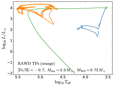
Figure 1: An example of stellar evolution tracks from our new RAWD simulations. The blue track shows the evolution of an initially $3\,$M_⊙ model from the pre-MS phase through to its first He-shell pulse on the AGB. The model is then forced to lose almost its entire H-rich envelope in a presumably common-envelope event and the remaining $0.72\,$M_⊙ CO core moves towards the WD cooling track (the green curve). The orange track with multiple loops shows the RAWD evolution that consists of H-accreting phase, followed by a He-shell thermal pulse (TP), envelope expansion, its loss via the Roche-lobe overflow, and return of the model to the accretion phase.

We have extended the RAWD simulations to the following lower initial chemical compositions: [Fe/H] $=0.0,\ -0.7,\ -1.1,\ -1.55$, and $-2.3$. We adopt the Asplund et al. (2009) solar abundance distribution which implies the heavy-element mass fractions $Z_{\mathrm{met}}=0.014,\ 0.0054,\ 0.0021,\ 0.00076$, and $0.00014$, respectively. Details of our new RAWD simulations will be presented elsewhere. Here, we are using only the $i$-process yields calculated for CO WD masses that are all close to $0.7\,$M_⊙. Figure 1 shows as an example the stellar evolution track for [Fe/H] $=-0.7$ computed with the MESA code (revision 7624 Paxton et al., 2013). The blue curve is a track of an initially $3\,$M_⊙ star from the pre-MS evolutionary phase through to its first He-shell flash on the AGB. After that, the model star is forced to lose its envelope, as if a common-envelope event occurred to it and, as a result, it leaves the AGB and moves to the WD cooling track (the green curve). The accretion of H-rich material begins after the $0.72\,$M_⊙ CO WD has cooled down to $\log_{10}L/L_{\odot}=-2$. We start with a slow accretion, $\dot{M}_{\mathrm{acc}}\sim 10^{-8}-10^{-9}\,$M${}_{\odot}\,\mathrm{yr}^{-1}$, more typical for novae, to ensure numerical convergence, and we switch to the rapid accretion at a later time. The orange curve shows the multiple loops that the evolutionary track of the RAWD makes when it experiences He-shell flashes followed by its expansion, mass loss due to the Roche-lobe overflow, and return to the mass-accreting phase. The pathway to RAWDs adopted for our yield calculations (Figure 1) is also present in our binary population synthesis models.

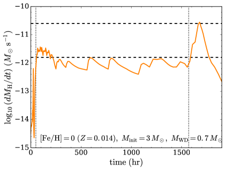
Figure 2: Rate and duration of H ingestion in the solar-metallicity RAWD model estimated from its H-burning luminosity. Note the final short phase with an increased rate of H ingestion that is typical for near-solar metallicity RAWD models.

For the $i$ process to be activated, the He-shell convection has to ingest some H from its surrounding H-rich envelope. In our 1D stellar evolution models of RAWDs this happens even if no convective overshooting is assumed (see Figure 2 in Denissenkov et al., 2017). When convective boundary mixing at the top boundary of the pulse-driven convection zone is included according to the exponentially decaying diffusive model with an efficiency $f=0.01$ as recommended by Herwig et al. (2007), the 1D RAWD models have H-ingestion rates of $\dot{M}_{\mathrm{H}}\sim 10^{-11}-10^{-12}\,$M${}_{\odot}\,\mathrm{s}^{-1}$, as estimated from their H-burning luminosities. These are consistent within a factor of 2 to those obtained in 3D hydro simulations of H ingestion by He-flash convection, using the convective He-shell structure and He-burning luminosities from our RAWD models (R. Andrassy, priv. com.). These values of $\dot{M}_{\mathrm{H}}$ have been used in our post-processing nucleosynthesis computations of the $i$ process in RAWDs. We have carried out these computations using the multizone frame mppnp of the NuGrid code (Pignatari et al., 2016). Durations of the H ingestion events have been estimated from our 1D RAWD models. In single post-AGB stars VLTPs induce a violent H ingestion that has a higher mass ingestion rate ($\dot{M}_{\mathrm{H}}\sim 10^{-10}\,$M${}_{\odot}\,\mathrm{s}^{-1}$) than in the preceding thermal pulse evolution. This high ingestion rate is only maintained for a short time (hundreds of minutes, Herwig et al., 2011), while in RAWDs H ingestion is usually 10 to 100 times slower, not accompanied by violent H burning or major perturbations of the convective structure of the He-shell, and it lasts tens of days. In the case of [Fe/H] $=0$, such a long-lasting gentle H ingestion is followed by a much shorter and stronger H-ingestion event that resembles the violent H ingestion after a VLTP and that terminates the whole H-ingestion process (Figure 2). We take this into account in our post-processing nucleosynthesis computations by changing $\dot{M}_{\mathrm{H}}$ appropriately in our solar-metallicity RAWD models.

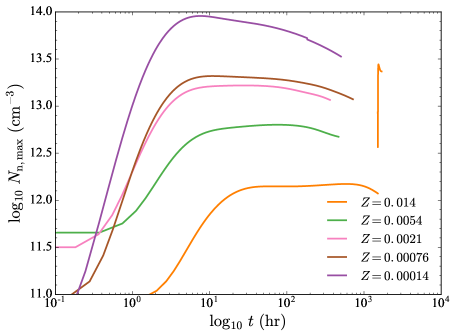
Figure 3: Maximum neutron densities in the He convective zones from the post-processing computations of the $i$-process nucleosynthesis in our RAWD models. The almost vertical part of the orange curve corresponds to the final fast H-ingestion event in the solar-metallicity RAWD model that is seen in Figure 2.

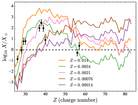
Figure 4: Distributions of element yields from the post-processing computations of the $i$-process nucleosynthesis in our RAWD models. The black circles with error bars are surface abundances in Sakurai’s object measured by Asplund et al. (1999). Note the high abundances of the first-peak elements in the nearly-solar metallicity models.

Figure 3 shows maximum neutron densities in the convective He shells of our post-processed RAWD models as a function of time. The orange curve consists of two parts, the second, almost vertical one, corresponding to the final strong H ingestion event that we have revealed in the solar-metallicity model (Figure 2). The peak value of $N_{\mathrm{n,\,max}}$ increases when the metallicity decreases because of a decreasing total mass fraction of the neutron-capture seeds. This results in a shift of the final distribution of $i$-process yields towards heavy elements (Figure 4). However, for the main topic of this work it is more important to comment on the RAWD yields of the first-peak elements with the charge number around $40$. The black circles with error bars in Figure 4 show the surface abundances in Sakurai’s object measured by Asplund et al. (1999). In terms of abundance distribution, the RAWD yields at near-solar metallicity contain similar or even higher amounts of first-peak elements compared to Sakurai’s object. Given that RAWDs can potentially undergo tens of He-shell flashes with low He-shell mass retention efficiencies, they can indeed be important contributors to the GCE evolution of these elements, as was originally proposed by Denissenkov et al. (2017).

Isotopes with large neutron-capture cross sections that act as neutron poisons are all automatically included in our nucleosynthesis computations. We begin with the abundance distributions in the He convective zones obtained from the solar-scaled abundances processed through complete H burning followed by partial He burning. The ingested material has the same initial solar-scaled chemical composition, and the NuGrid codes that we use take into account all the relevant reactions ($\sim$ $14{,}000$ reactions for the models presented in Figure 4 and $\sim$ $61{,}000$ for test runs).

The RAWD $i$-process elemental yields from Figure 4 supplemented by their corresponding isotopic yields are used as input data for the GCE model described in Section 4. These yields represent decayed elemental and isotopic abundances mass-averaged over convective He shells.

3 Population Synthesis Model

Our binary star populations that give rise to the RAWD systems are simulated with the StarTrack rapid binary evolution population synthesis code (Belczynski et al., 2002, 2008). We simulate stellar populations from the zero-age main sequence (ZAMS) up to a Hubble time. Assuming a binary fraction of 70%, all stars are born in a starburst at $t=0$, and later convolved with the appropriately-chosen star formation history and star formation efficiency (see Section 4). Our four populations are evolved using four different ZAMS metallicities: $Z_{\mathrm{met}}=0.02$, 0.002, 0.001, and 0.0001. The effect of initial metallicity on the binary evolution, and thus on the RAWD birthrates, is discussed in Section 6.2.

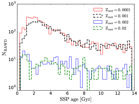
Figure 5: Number of rapidly accreting white dwarfs (RAWDs) occurring in a simple stellar population (SSP) as a function of time, split into 50 bins. Different colors represent population synthesis predictions at different metallicity $Z_{\mathrm{met}}$ (see Section 3). Each SSP has a total stellar mass of $3.2\times 10^{6}$ $M_{\sun}$, which is formed instantaneously. In total, $1.58\times 10^{-3}$, $1.26\times 10^{-3}$, $1.0\times 10^{-4}$, and $8.9\times 10^{-5}$ RAWD event occurs per unit of stellar mass formed at $Z_{\mathrm{met}}=0.0001$, 0.001, 0.002, and 0.02, respectively. We refer to Annexe A for a discussion of the sharp transition between $Z_{\mathrm{met}}=0.001$ and 0.002.

Initial ZAMS star masses are drawn from the 3-component power-law initial mass function of Kroupa et al. (1993) with $\alpha_{1}=-1.3$, $\alpha_{2}=-2.2$, $\alpha_{3}=-2.35$. The initially more massive star ($M_{1}$) and its companion ($M_{2}$) are chosen within the mass range of $0.8-100.0$ and $0.5-100$ $\mathrm{M}_{\odot}$, respectively. $M_{1}$ is drawn directly from the probability distribution function given by our chosen IMF while $M_{2}$ is calculated by randomly picking a mass ratio $M_{2}/M_{1}$ between 0 and 1. (Duquennoy & Mayor, 1991; Toonen et al., 2014, but see also Moe & Di Stefano 2017). For simplicity, we assume circular orbits from the ZAMS and flat orbital separations (in the logarithm) from $2\times$($R_{1}+R_{2}$) to $10^{5}$ $\mathrm{R}_{\odot}$ (standard prescription).

Interacting binary stars undergo at least one common envelope (CE) phase over the course of their evolution. Though this phase is extremely important in bringing two stars close enough to one another to undergo mass transfer, it is one of the most poorly-understood processes in stellar astrophysics (see Section 6.1). In population synthesis studies, the CE phase cannot be explicitly calculated but must be parametrized in some way. A common approach is to equate the binding energy of the envelope of the mass-losing star, $E_{\rm bind}=GM_{\rm core}M_{\rm env}R^{-1}\lambda^{-1}$ (see below), with the orbital energy of the binary system. The envelope will then be expelled from the system at the expense of the binary’s orbital energy, which causes the orbital size to decrease, often drastically. We adopt the “standard” common envelope formalism employing energy balance (Webbink, 1984) that is often used in binary population synthesis codes with $\alpha_{\rm CE}\times\lambda=1$ (see Ruiter et al., 2009). Here, $\alpha_{\rm CE}$ is the fraction of orbital energy that is used to eject the envelope of the mass-losing star, and $\lambda$ is the binding energy parameter.

We consider a sub-population of our accreting white dwarfs to contribute to the RAWD population. Specifically, any CO WD with a mass $\geq 0.6$ $\mathrm{M}_{\odot}$ that accretes from any hydrogen-rich star at a rate $\geq 3.066\times 10^{-7}[(M_{\rm WDaccretor}/\mathrm{M}_{\odot})-0.5357$] $\mathrm{M}_{\odot}$ yr^-1 (Nomoto et al., 2007, see their Figure 4) is considered to be a RAWD in our models. For this study, unlike in previous studies (e.g. Ruiter et al., 2009), we artificially suppress hydrogen accumulation on the WD, as found in Denissenkov et al. (2017). The implications of this for other sources, such as Type Ia supernovae (SNe Ia), are discussed in Section 6.3. The time (from star formation) when these accretion criteria are satisfied is considered to be the RAWD birth time (its “delay time”). The delay time distribution (DTD) functions for the 4 RAWD populations are shown in Figure 5 and set the enrichment timescale of $i$-process element that are implemented in our GCE model.

4 Milky Way Model

In this section we briefly describe our galactic chemical evolution model and compare its output properties with the Milky Way.

4.1 Galactic Chemical Evolution Code

We use the one-zone chemical evolution code OMEGA described in Côté et al. (2017a), which is available on GitHub as part of the open-source NuGrid Python Chemical Evolution Environment (NuPyCEE, version 2.0). From an input star formation history, which is decreasing with time in our case, the code follows the contribution of several simple stellar populations (SSPs) to the overall stellar ejecta by keeping track of the age, initial metallicity, and initial mass of each SSP. OMEGA uses the uniform-mixing approximation and accounts for galactic outflows and primordial inflows. The rate of inflow at each timestep is automatically adjusted to sustain the input star formation rate. Our code offers a variety of parametrization options for outflows and star formation efficiencies. But in this work, we use the option described in Côté et al. (2016) which allows to control the early chemical evolution of the galactic gas independently of its final properties. As seen in Section 4.3, this enables us to explore different chemical evolution paths to reach solar composition and to quantify the confidence levels of the predicted contribution of RAWDs.

We use the NuGrid Set1 extension stellar yields (Ritter et al. 2017b) for asymptotic giant branch (AGB) stars and massive stars including core-collapse supernova nucleosynthesis (see Pignatari et al. 2016). Stellar models are provided at five metallicities from 0.0001 to 0.02 in mass fraction. We also use the yields of Heger & Woosley (2010) for zero-metallicity stars and the W7 model of Iwamoto et al. (1999) for SN Ia yields. We use the stellar initial mass function of Kroupa (2001) for all stellar populations at all metallicities. However, the choice of stellar yields is not particularly important for this work since we are only interested in the evolution of $Z_{\mathrm{met}}$, the overall gas metallicity (see Section 4.3).

Table 1: Properties of our galaxy model (OMEGA) at the end of the simulation compared to current disk properties of the Milky Way taken from Table 1 in Kubryk et al. (2015, K15). SFR, CC SN, and SN Ia stand for star formation rate, core-collapse supernova, and Type Ia supernova.

Quantity	OMEGA	Milky Way (K15)
Stellar mass [1010 $M_{\odot}$]	5.0	3 – 4
Gas mass [109 $M_{\odot}$]	9.1	$8.1\pm 4.5$
SFR [$M_{\odot}$ yr-1]	2.5	0.65 – 3
Inflow rate [$M_{\odot}$ yr-1]	1.4	0.6 – 1.6
CC SN rate [per 100 yr]	2.5	$2\pm 1$
SN Ia rate [per 100 yr]	0.3	$0.4\pm 0.2$

We refer to Côté et al. (2017a) for more information on OMEGA and to Ritter et al. (2017a) for more information on the implementation of SSPs and SNe Ia.

4.2 RAWD Implementation

The contribution of RAWDs has been implemented in our SSP module SYGMA (Ritter et al., 2017a), which is called at each timestep by OMEGA. Because the gas metallicity increases continuously in our one-zone galaxy model, each formed SSP has a unique metallicity and thus has a unique set of $i$-process yields and DTD function for their RAWDs population. The yields are interpolated in the log-log space in order to represent the initial metallicity of the stars. The DTD functions are also interpolated to provide a continuous evolution of RAWD rates as a function of galactic age. The total number of RAWD events in an SSP depends on its total mass and on the normalization of its interpolated DTD function. At a given timestep in our simulation, the overall RAWD ejecta is calculated by summing the contribution of all existing SSPs and by keeping track of their specific age, mass, and unique set of interpolated $i$-process yields and DTD function.

Each RAWD event is assumed to eject between 0.5 and 1 M_⊙ of material. Our binary population synthesis simulations find $0.86\,M_{\odot}$ and $1.2\,M_{\odot}$ for the mean masses of the RAWD and its donor. The isotropic re-emission approximation (see Section 3.3.3 in Postnov & Yungelson, 2014, and references therein), that is appropriate for our RAWD binary models, provides a stable mass transfer for the accretor to donor mass ratio $q\lesssim q_{\mathrm{crit}}\approx 1$. This means that our RAWD models with the masses $\sim 0.7\,M_{\odot}$ should be able to stably accrete up to $\sim 0.5\,M_{\odot}$ from their $1.2\,M_{\odot}$ companion. The $0.86\,M_{\odot}$ RAWDs would accrete $\sim 0.34\,M_{\odot}$. We think that our estimates of the total ejected mass have a factor of $\sim 2$ uncertainty. The accretion itself usually takes a few Myr for $q$ to reach its critical value.

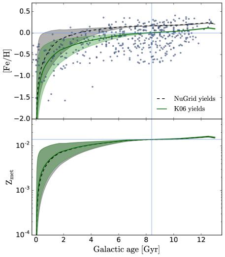
Figure 6: Evolution of [Fe/H] (upper panel) and metallicity $Z_{\mathrm{met}}$ in mass fraction (lower panel) as a function of Galactic age. The black dashed and green solid lines represent our numerical predictions using NuGrid (Ritter et al. 2017b) and Kobayashi et al. (2006, K06) yields. For each set of stellar yields, the shaded area shows the different chemical evolution paths that can be predicted by our one-zone model at early times. These variations are used to provide confidence levels in the predicted contribution of rapidly accreting white dwarfs (see Section 5). The horizontal blue lines show the solar metallicity (Asplund et al. 2009). The vertical blue line going across the two panels show the time at which the Sun is assumed to form in our model, 4.6 Gyr (Connelly et al., 2017) before the end of the 13 Gyr-long simulation. Observational data was taken from Bensby et al. (2014, blue dots). Error bars for [Fe/H] data are about 0.05 dex while the ones for Galactic age data can reach several Gyr. We reversed the time axis in the data so that the shortest look-back time found in Bensby et al. (2014) corresponds to the end of our simulation. We did not include data with large uncertainties (grey dots in their Figure 21).

4.3 Milky Way Properties

The focus of this paper is the chemical composition of the Galactic gas when the Sun forms. We have tuned our chemical evolution model to ensure that the gas reaches solar metallicity ($Z_{\mathrm{met},\odot}=0.014$, Lodders et al. 2009) 4.6 Gyr before the end of the simulation, which lasts for 13 Gyr. We also tuned our model to roughly reproduce the current observed properties of the Milky Way (see Table 1). The upper panel of Figure 6 shows the predicted evolution of [Fe/H] as a function of Galactic age. The dashed black and green solid lines represent our fiducial predictions using different sets of stellar yields. The shaded areas highlight the different chemical evolution paths to reach the Sun with our model. These different paths are use to test the sensitivity or our results (see Section 5).

As described in Côté et al. (2016), we can modify the gas content at early times (which modifies the metal concentration) without modifying the final properties of our galaxy model and the overall metallicity from which the Sun forms (lower-panel of Figure 6). Because the contribution of SNe Ia in the Milky Way should appear near [Fe/H] $\sim-1$ (e.g., Matteucci & Greggio 1986; Chiappini et al. 2001), the lower limit for the evolution of [Fe/H] was chosen so that a value of $-1$ is reached at most after 1 Gyr of evolution. This represents a comfortable lower limit given the prompt nature of SNe Ia (e.g., Mannucci et al. 2005; Li et al. 2011) and their minimum delay times of ${\sim}10^{8}$ Myr (e.g, Ruiter et al. 2011; Heringer et al. 2017).

The choice of stellar yields for massive stars affects the scaling of [Fe/H]. Our SSPs tend to eject more Fe with NuGrid yields compared to when we use the ones found in Kobayashi et al. (2006) (see also Philcox et al. 2017). The choice of stellar yields, however, does not significantly impact the overall metallicity evolution in the Galactic gas (lower-panel of Figure 6). Because the goal of this paper is to quantify the contribution of RAWDs to the solar composition, our results are insensitive to the adopted stellar yields, since the predicted RAWD ejecta only depends on the overall metallicity, and not on its elemental composition.

5 Results

In the following sections, we describe our predicted Galactic RAWD rates and their contribution to the elemental and isotopic compositions of the Sun.

5.1 RAWD Rates

The upper panel of Figure 7 shows the RAWD birth rates as a function of Galactic age. The rates are most uncertain at early times and vary by an order of magnitude at 2.5 Gyr. This peak of uncertainty is caused by the sharp transition at $Z_{\mathrm{met}}=0.001-0.002$ above which RAWD rates in SSPs drop by an order of magnitude (Figure 5). The time for the Galactic gas to reach this transition metallicity depends on the chosen chemical evolution path (Figure 6). When the metallicity of the gas evolves slowly, more low-metallicity SSPs will be formed, which will increase the RAWD rates. On the other hand, when the metallicity of the gas evolves rapidly, SSPs will be more metal-rich on average and RAWD formation will be somewhat suppressed (Figure 5).

In all the considered chemical evolution paths, the sharp transition metallicity mentioned above is reached within the first Gyr of evolution (see Section 4.3), which is why the scatter in the Galactic rate decreases after 2.5 Gyr. The level of scatter stays relatively constant beyond solar metallicity (blue vertical line in Figure 7) since we did not calculate yields and DTD functions for RAWDs at $Z_{\mathrm{met}}>0.014-0.02$. Because our target observable is the Sun, we did not need to follow the GCE calculation beyond the adopted solar value. When the metallicity of the gas reached solar, we simply applied the highest-metallicity yields and rate for all subsequent SSPs that formed at later times. Our predictions for the current Galactic RAWD rates are higher by a factor of $2-3$ compared the lower limit estimated by Denissenkov et al. (2017) that were based on population synthesis predictions (Chen et al. 2014) for the single-degenerate SN Ia scenario (see also Ruiter et al. 2009).

The lower panel of Figure 7 shows the cumulated number of RAWDs in our simulation as a function of Galactic age. Because of the different chemical evolution paths assumed at early times, the predicted number of RAWDs that contribute to the solar composition varies by a factor of $\sim$ 3.5.

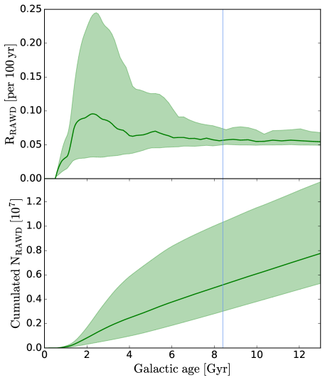
Figure 7: Predicted rate (upper) and cumulated number (bottom) of rapidly accreting white dwarfs (RAWDs) as a function of Galactic age. The green solid lines represent our fiducial model while the green shaded areas show the range of solutions generated by different chemical evolution paths (see Figure 6).

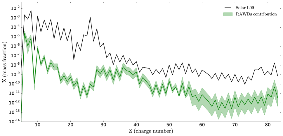
Figure 8: Predicted contribution of rapidly accreting white dwarfs (green, RAWDs) to the elemental solar composition (black). The green solid line represents our fiducial model while the green shaded area shows the range of solutions generated by uncertainties in the total mass ejected by RAWDs (see Section 4.2) and by different early chemical evolution paths (see Figure 6). The solar composition was taken from Lodders et al. (2009, L09).

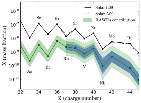
Figure 9: Same as in Figure 8, but zoomed on first-peak elements. The dashed black line shows the solar composition of Asplund et al. (2009, A09). The blue shaded area shows the uncertainties generated by nuclear reaction rates (see Section 6.4). The larger lighter-green shaded area shows the combined uncertainties generated by different chemical evolution paths, different ejecta masses for each RAWD, and by nuclear reaction rate uncertainties.

5.2 Elemental Composition

Figure 8 shows the predicted contribution of RAWDs to the chemical composition of the Galactic gas when the Sun forms, 4.6 Gyr before the end of the simulation. The green solid line represents our fiducial chemical evolution path (see dashed line in the bottom panel of Figure 6) assuming 0.75 M_⊙ for the integrated $i$-process ejecta over the lifetime of each RAWD. The green shaded area shows the range of solutions generated by using different chemical evolution paths (Figure 6) and different ejecta masses between 0.5 and 1 M_⊙. This level of uncertainty varies from one element $Z$ to another because of the metallicity-dependent rates and yields adopted for RAWDs.

The level of uncertainty is systematically higher at $Z\gtrsim 55$. When the chemical evolution path favours low-metallicity SSPs ($Z_{\mathrm{met}}<0.002$), which occurs when the metallicity of the Galactic gas evolves slowly, there will be more RAWDs because of the higher birthrates predicted by our population synthesis model (Figure 5). In addition, our RAWD yields at $Z_{\mathrm{met}}<0.002$ mainly produce elements with $Z\gtrsim 55$ (Figure 4). The opposite situation occurs when the chemical evolution path favours high-metallicity SSPs ($Z_{\mathrm{met}}>0.002$). In that case, there will be less RAWDs along with a lack of nucleosynthetic production for $Z\gtrsim 55$.

The situation is different for lighter elements (e.g, $Z=[30-55]$). When low-metallicity SSPs are favoured, although more RAWDs will form compared to high-metallicity SSPs, less $Z\lesssim 55$ elements will be ejected per RAWD event (Figure 4). When high-metallicity SSPs are favoured, more $Z\lesssim 55$ elements will be ejected per RAWD event, but less RAWDs will form in total. To summarize, there is a cancelation effect in the mass of $Z\lesssim 55$ elements ejected in the Galactic gas: high RAWD rates imply low nucleosynthetic yields, and vice-versa. On the other hand, there is an amplification effect for the heavier $Z\gtrsim 55$ elements (see paragraph above), which explains the larger spread seen for the heaviest elements in Figure 8.

Overall, the contribution of RAWDs to the solar composition is not significant except for elements near the first peak ($Z=[36-42]$). Figure 9 shows a zoom of the region of interest. According to our model, even though RAWDs are not the dominant contributor to the production of these elements, their contribution is still significant and could explain the origin of a fraction of the solar first-peak composition (see Table 2).

Table 2: Predicted contribution, in percentage, of rapidly accreting white dwarfs (RAWDs) to the first-peak elemental solar composition of Asplund et al. (2009, A09) and Lodders et al. (2009, L09). The fiducial values represent the solid green line in Figure 9. The values in bracket show the range of plausible solutions if we account for different galactic chemical evolution (GCE) paths, nuclear reaction rate uncertainties (Nucl. React.), and for both sources of uncertainties combined. We described how we combined uncertainties at the end of Section 5.2.

Z	Element	RAWDs contribution [%]
		Fiducial (L09)	GCE (L09)	Nucl. React. (L09)	Combined (L09)	Combined (A09)
35	Br	2.5	[ 0.9 - 6.3 ]	—	[ 0.9 - 6.3 ]	—
36	Kr	5.9	[ 2.2 - 15.2 ]	—	[ 2.2 - 15.2 ]	[ 2.3 - 16.2 ]
37	Rb	17.1	[ 6.3 - 43.4 ]	[ 10.8 - 27.0 ]	[ 4.0 - 68.6 ]	[ 2.9 - 49.7 ]
38	Sr	4.0	[ 1.5 - 9.9 ]	[ 2.3 - 6.9 ]	[ 0.9 - 17.1 ]	[ 0.9 - 18.3 ]
39	Y	8.0	[ 3.0 - 20.5 ]	[ 4.0 - 15.8 ]	[ 1.5 - 40.5 ]	[ 1.5 - 39.6 ]
40	Zr	7.8	[ 3.0 - 20.3 ]	[ 4.5 - 13.5 ]	[ 1.8 - 35.2 ]	[ 1.7 - 34.4 ]
41	Nb	5.7	[ 2.2 - 14.7 ]	[ 1.5 - 21.6 ]	[ 0.6 - 56.0 ]	[ 0.5 - 51.0 ]
42	Mo	8.1	[ 3.3 - 21.2 ]	[ 3.3 - 19.5 ]	[ 1.4 - 51.2 ]	[ 1.6 - 58.7 ]
44	Ru	1.7	[ 0.7 - 4.4 ]	[ 0.7 - 4.2 ]	[ 0.3 - 11.1 ]	[ 0.3 - 11.8 ]

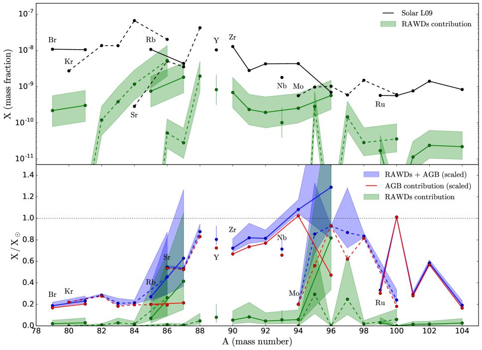
Figure 10: Upper: Same as in Figure 9, but decomposed in isotopic compositions. The solar isotopic composition found in Lodders et al. (2009, L09) are the same as in Asplund et al. (2009). The alternance between solid and dashed lines is to help keeping track of the isotopes with the same charge number. Lower: Contributions of AGB stars Cristallo et al. (2015b, $s$-process, red lines), RAWDs (green lines), and the sum of AGB and RAWDs (blue lines), in mass fraction relative to the solar composition (black dotted line). The AGB stars contribution has been reduced by 35% so that the $s$ process produces 100% of ¹⁵⁰Sm, an $s$-only isotope.

As shown in Figure 9 and Table 2, nuclear reaction rate and galactic chemical evolution uncertainties affect our results in a similar way. To include nuclear reaction rate uncertainties in our fiducial prediction (blue shaded area in Figure 9), we used the 1-$\sigma$ dispersions extracted from normal distributions generated by Monte Carlo calculations (see Section 6.4). The same dispersions have been applied to our lower and upper limit predictions, which were produced by assuming different chemical evolution paths and ejecta masses, in order to estimate the combined uncertainties (larger and lighter green shaded area).

5.3 Isotopic Composition

The upper panel of Figure 10 shows the contribution RAWDs to the isotopic composition of the solar composition for the same elements shown in Figure 9. Our predictions do not overproduce any isotope, except for ⁹⁶Zr which is produced in a similar quantity than what is observed in the Sun. In general, the isotope production patterns of our $i$-process yields do not follow the solar composition.

In the bottom panel of Figure 10, we divided our predictions by the solar composition and compare the RAWDs contribution with the $s$-process isotopic pattern predicted by our fiducial GCE model using the non-rotating AGB stars yields from the FRUITY database (Cristallo et al. 2015b). We scaled down the $s$ process by 35 % so that it accounts for 100 % of the ¹⁵⁰Sm observed in the Sun, which is an $s$-only isotope. This normalization is consistent with Cristallo et al. (2015a) who also noticed an overestimation of about 45 % for $s$-only isotopes using their non-rotating AGB yields, but using a different GCE code. Using their rotating AGB models would likely underestimate ¹⁵⁰Sm (see their Figure 6). We do not include the isotopic composition of the $r$ process because of the large uncertainties associated with theoretical calculations (e.g., Martin et al. 2016; Mumpower et al. 2016). Using the $r$-process residuals as an alternative solution would leave, by definition, no room for the $i$ process.

The blue lines represent the combined contribution of RAWDs and AGB stars. Uncertainties in the yields of AGB stars is not included in this panel. In some cases, as shown in the bottom panel of Figure 10, the $i$ process (green lines) has a production peak where the $s$ process (red lines) has a local minima (e.g., ⁹⁶Zr, ⁹⁷Mo). In the case of ⁹⁶Mo, the $i$ process shows a local minima while the $s$ process shows a global maxima. Although isotope yields for RAWD and AGB models need to be addressed with quantified uncertainties, which is beyond the scope of this paper, Figure 10 suggests that the $i$ process can complement the $s$ process for some isotopes.

As an example, ⁹⁵Zr represents a branching point (e.g., see Lugaro et al. 2014; Battino et al. 2016) which means that there is a probability to capture a neutron and form the stable ⁹⁶Zr isotope, depending on the neutron density. During the $i$ process, the neutron density is higher than with the $s$ process and unstable ⁹⁵Zr isotopes are more efficiently transformed into ⁹⁶Zr, which leads to a higher ⁹⁶Zr abundance compared to the $s$-process case.

6 Discussion

Here we discuss the various sources of uncertainties unaccounted in our results and the limitations of our galactic chemical evolution code to quantify the contribution of RAWDs to the solar composition. We also discuss the implications of our results on the solar LEPP and on the single-degenerate SN Ia scenario.

6.1 Common Envelope Evolution

In the adopted (energy balance) common envelope formalism (see Section 3), the $\alpha_{\rm CE}$ and $\lambda$ parameters contain a lot of “unknown physics” and the assumptions made during this phase are one of the largest sources of uncertainty in our models (see Ivanova et al., 2013; Toonen et al., 2014). Higher values of $\alpha_{\rm CE}\times\lambda$ means higher ejection efficiencies which leads to wider orbital separations following the ejection of the CE. In general, choosing different reasonable values for these quantities could affect our results, but not in a drastic way. For example, if the physical processes leading to the unbinding of the CE were less efficient (e.g. lower $\alpha_{\rm CE}$ or $\lambda$ values), some fraction of the “standard” binaries would not make RAWDs, as they would follow a different evolution that may cause them to merge too early on. However, binaries that would not have become RAWDs in our standard model, since they were not brought close enough together after the CE, would likely populate this RAWD parameter space instead.

6.2 Effect of Metallicity on RAWD Birthrates

We have shown that at higher ($\sim$solar) metallicities, the RAWD birthrate is about 10 times lower than for lower metallicities (Figure 5). As described below, this is due to a combination of effects, which include metallicity-dependent stellar winds and different mass ratios for the stars when the companion transfers hydrogen towards the WD.

One side effect of metallicity-dependent wind mass loss is that the lower-metallicity WDs will be more massive than their higher-metallicity counterparts, since the star was able to maintain larger (core) mass during later stages of stellar evolution. As a consequence, at time of Roche-Lobe overflow (RLOF) between the H-rich (e.g. Hertzsprung Gap) companion and the CO WD, lower metallicity systems have less extreme mass ratios. The less extreme mass ratio between the WD and the H-burning star is what enables these systems to undergo (quasi) stable mass transfer, and thus evolve into RAWD binaries. On the other hand, the higher-metallicity binaries have more extreme mass ratios at time of RLOF, which makes it more likely for them to encounter mass transfer on a dynamical timescale (e.g. CE evolution).

As noted in Section 3, there is a rather extreme decrease in RAWD birthrate between $Z_{\mathrm{met}}=0.001$ and 0.002. Many systems which would make RAWDs involving evolved companions in the lower $Z_{\mathrm{met}}$ (0.0001, 0.001) models will make detached double WDs in the higher $Z_{\mathrm{met}}$ (0.002, 0.02) models consisting of a CO WD and a helium WD (due to stripping of the H-envelope during CE evolution). The reason why the rate difference is notably extreme between our $Z_{\mathrm{met}}=0.001$ and $Z_{\mathrm{met}}=0.002$ models is because of a transition region within our StarTrack algorithm that is used to determine whether a system in RLOF will encounter mass transfer on a thermal or dynamical timescale (Belczynski et al., 2008, see section 5).

We note that our algorithm that calculates the stability of mass transfer is uncertain, though star systems have indeed been observed to undergo a phase of quasi-stable mass transfer prior the (expected) CE phase, at least in massive stars. If this same analogy can be applied to lower-mass stars, we may be underestimating the RAWD birthrates at high metallicities, in which case our imposed criteria for undergoing a CE should be revised to allow the production of more RAWDs at more extreme stellar mass ratios. In Annexe A, we explore an alternative set of GCE predictions where the RAWD birthrate smoothly evolves as a function of metallicity without a sharp transition.

There is another reason why higher-metallicity systems do not produce as many RAWDs, which is applicable to a different evolutionary channel (WD+MS RAWD): some higher-metallicity binaries are more readily destroyed via mergers during the first mass transfer event when the primary is on the RGB and the secondary is still on the MS. For the lower-metallicity counterpart, the (smaller in radius) primary would have already reached the early AGB and thus would have a larger core mass than the higher-metallicity RGB primary counterpart, despite the lower wind-mass loss rates in the lower-metallicity model. Both star systems will go to CE, but only the low-metallicity system will survive, leaving behind a He-burning sub-giant and a MS star, which eventually evolves into a RAWD. The higher-metallicity system that has the more extreme mass ratio (between core and MS star) will end up as a merger between a compact He-burning core and a MS star.

6.3 Implications of Mass Retention Efficiency on the Type Ia Supernova Rate

One of the leading progenitor scenarios of SNe Ia includes the ‘textbook’ single degenerate (SD) scenario, in which a CO WD approaches the Chandrasekhar mass limit via accretion from a (usually hydrogen-rich) stellar companion. Studies tracking the theoretical evolution of interacting binary populations have shown that it is difficult for a CO WD to build up to the Chandrasekhar mass via hydrogen accretion (e.g., Ruiter et al., 2009; Bours et al., 2013, but see Han & Podsiadlowski 2004). In addition, recent works have shown that some, if not most, SN Ia explosions may be more easily explained by exploding sub-Chandrasekhar mass WDs, either via mergers, or ‘classic’ double-detonations (Pakmor et al., 2012; Shen et al., 2013; van Rossum et al., 2016; Sato et al., 2016; Shappee et al., 2017, see also Maguire et al. 2016). Despite the recent favouritism for sub-Chandrasekhar mass models (see also McWilliam et al. 2017), the Chandrasekhar mass SD scenario (sometimes referred to as the delayed detonation scenario Ciaraldi-Schoolmann et al., 2013) still remains a viable progenitor candidate (e.g., Wheeler, 2012; Seitenzahl et al., 2013; Fisher & Jumper, 2015; Yamaguchi et al., 2015; Hitomi Collaboration, 2017). However, the measurement of nebular emission lines in different galaxies implies a limit on the contribution of the SD scenario to the overall observed SNe Ia rate to less than $\sim 10$ % (Johansson et al. 2014, 2016, see also Woods et al. 2017 and Botyánszki et al. 2018).

In our adopted accretion model for RAWDs, where accretion on CO WDs is suppressed at relatively high mass transfer rates (see Section 3), it would be (nearly) impossible to produce any SNe Ia via the ‘textbook’ SD channel where a hydrogen-rich donor transfers mass via stable RLOF. We do find however a relatively small number of CO WDs that accrete up to the Chandrasekhar mass via wind accretion when the donor is an AGB star. These systems undergo a different evolutionary channel from RAWDs, where RLOF phases occur between an evolved star and a MS companion, so they never enter the RAWD parameter space.

When the primary star turns into a CO WD, it is already fairly close to the Chandrasekhar mass (${\sim}1.38$ $\mathrm{M}_{\odot}$), and futher accretion by the AGB companion wind is able to push the WD toward the Chandrasekhar mass. We predict that these SN Ia progenitors, if realised in nature, have prompt delay times ($<100$ Myr), and only occur in higher metallicity populations ($Z_{\rm met}\geq 0.002$). The lower metallicity primary stars (which experience less wind mass loss) are more likely to evolve into ONe WDs rather than CO WDs. We note that our current study cannot rule out near-Chandrasekhar mass explosions via RLOF from helium-rich companions, which have been proposed as good candidates for thermonuclear supernovae, in particular the fainter SN Iax-likes (Kromer et al., 2015; Stritzinger et al., 2015)

6.4 Yield Uncertainties

The $i$-process yields predicted with the RAWD models (Figure 4) depend on stellar physics and nuclear reaction rate uncertainties that are translated into yield uncertainties. Various stellar physics uncertainties will be analyzed elsewhere, and in that paper we will provide a detailed discussion of our RAWD models. Here, we only report some results on the yield uncertainties that are linked to the uncertainties of the (n,$\gamma$) cross sections of unstable isotopes near the magic neutron number $N=50$ and that are relevant to our predicted contribution of RAWDs to the solar first-peak elemental abundances (all details of the corresponding uncertainty study are presented in Denissenkov et al. 2016). These results have been obtained for a model of Sakurai’s object, whose $i$-process yields are similar to those of RAWD models with a nearly solar metallicity (Figure 4 in Denissenkov et al., 2017). The following paragraphs give a brief description of what has been done.

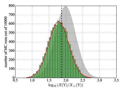
Figure 11: A distribution of the predicted abundance of Y (mass fraction) from our MC simulations in which we randomly varied the (n,$\gamma$) cross sections of 52 unstable isotopes near $N=50$ (the green histogram). The vertical dashed line is the benchmark model prediction for the reaction-rate multiplication factors $f_{i}=1$. By fitting a normal distribution (the red curve), we estimate the mean and dispersion of the results. For comparison, the grey-shaded area shows the observed Y abundance represented by a normal distribution with the mean and dispersion from Asplund et al. (1999).

First, 52 unstable isotopes of Br, Kr, Rb, Sr, Y, and Zr, whose (n,$\gamma$) cross sections can potentially affect the predicted abundances of Rb, Sr, Y and Zr, that were also measured in Sakurai’s object by Asplund et al. (1999), have been selected from the chart of nuclides. Because there is no experimental information on the (n,$\gamma$) cross sections of these isotopes, the Hauser-Feshbach model of a statistical decay of a compound nucleus was used to obtain it. When systematically varying between available five nuclear level density models and four $\gamma$ ray strength function parametrizations within the Hauser-Feshbach code, the largest and smallest n-capture rates were found and their ratios were assigned to the maximum variation factors $v_{i}^{\mathrm{max}}$ for all of the 52 isotopes.

Second, we have carried out Monte-Carlo (MC) simulations in which the $i$-process nucleosynthesis in Sakurai’s object was modeled 10,000 times with randomly selected sets of multiplication factors $f_{i}$ for the (n,$\gamma$) reaction rates involving the 52 selected isotopes (the benchmark model, with which we compared the results of our MC simulations, had all $f_{i}=1$). For each of the 52 isotopes in each of the 10,000 MC runs, we first selected a random number $v_{i}^{\mathrm{rand}}$ from a uniform distribution in the interval $1\leq v_{i}^{\mathrm{rand}}\leq v_{i}^{\mathrm{max}}$, then the multiplication factor was assigned a value of $f_{i}=(p/v_{i}^{\mathrm{rand}})+(1-p)v_{i}^{\mathrm{rand}}$, where $p$ were assumed to take a value of 0 or 1 with an equal probability.

The green histogram in Figure 11 shows a distribution of the predicted abundance of Y from our MC simulations. Similar histograms were constructed for the other elements of the fist peak. By fitting them with normal distributions, we were able to estimate their mean values and dispersions. For Rb, Sr, Y, Zr, Nb, Mo, and Ru, the (n,$\gamma$) reaction rate uncertainties of the 52 unstable isotopes are translated into the predicted yield uncertainties of 0.20, 0.24, 0.30, 0.24, 0.58, 0.38, and 0.40 (for the distributions of the logarithmic abundance ratios with respect to the initial or solar abundances). For the first four elements, these uncertainties turn out to be less than or comparable to their observed errors from Asplund et al. (1999). For the rest three elements, the estimated uncertainties do not include a contribution from the (n,$\gamma$) reaction rate uncertainties of unstable isotopes heavier than Zr, therefore they can in fact be (probably, slightly) different. Nevertheless, we used all of these data in the analysis of our predicted contribution of RAWDs to the solar first-peak elemental abundances.

6.5 Galaxy Evolution Uncertainties

Because the yields and rates used for RAWDs are metallicity-dependent, our results are affected by the chemical evolution path used in our Milky Way model. The overall evolution of metallicity as a function of time in a one-zone model is driven by the shape of the star formation history (SFH) and by the amount of gas in which stellar ejecta are deposited. The latter is controlled by the star formation efficiency. As shown in Figure 6, it is possible to create different chemical evolution paths using the same SFH but by varying the star formation efficiency. But the shape of the SFH also plays an important role in GCE, as it defines how many SSPs are formed at a specific metallicity and how fast the galactic gas is being enriched. Indeed, as shown in Fenner & Gibson (2003), different SFHs can also lead to different chemical evolution paths at early times (see also Hirai et al. 2017).

In this work, we only varied the star formation efficiency, but any variation from what we assumed for the SFH could change the predicted number ratio of low- to high-metallicity SSPs and thus affect our predictions. This source of uncertainty has also been discussed by Cristallo et al. (2015a) in the context of metallicity-dependent AGB star yields. As explained in Sections 5.1 and 5.2, our results are sensitive to the age-metallicity relationship, and thus the SFH, during the first Gyr of evolution. Within a cosmological context, the SFH of galaxies in the early universe is significantly affected by structure formation and by galaxy mergers (e.g., Wise et al. 2012). The stochastic early phase of the Milky Way is still not well constrained, and our one-zone model is not suited to address this complexity (but see Côté et al. 2017b).

In addition, the concept of a direct correlation between age and metallicity breaks down at very low metallicity. Hydrodynamic simulations have shown that non-uniform mixing of stellar ejecta at early times generate significant scatter in the age-metallicity space (e.g., Wise et al. 2012; Hirai et al. 2015; Starkenburg et al. 2017). Accounting for more metallicity dispersion in our model would modify the metallicity range associated with our SSPs, which could affect the predicted contribution of RAWDs, given their strong dependency on metallicity. However, it is difficult with our model to evaluate whether those non-uniformities would significantly affect our results compared to an averaged uniformly-mixed model.

By using a one-zone model, we do not account for the formation timescale of different Galactic components such as the halo, the thick disc, and the thin disc. With multi-zone models (e.g., Ferrini et al. 1992; Pardi et al. 1995; Travaglio et al. 1999; Bisterzo et al. 2014), the formation of the Galactic disc is delayed relative to the formation of the halo. Assuming our one-zone model represents the Galactic disc, the time at which we form the Sun could be reduced by $\sim$ 1 Gyr, which is the typical delay for disc formation (Pardi et al. 1995; Chiappini et al. 2001). According to the bottom panel of Figure 7, this formation delay would change the total number of RAWDs included in the solar composition by no more than 20%, assuming the same star formation history.

6.6 Solar Lighter Element Primary Process

By combining the $r$ process and the weak and main $s$ processes in a galactic chemical evolution context, the solar composition near the first peak up to Xe is not fully explained without introducing an additional lighter element primary process, the so-called LEPP (Travaglio et al. 2004; Montes et al. 2007). This claim has later on been confirmed by Bisterzo et al. (2014). According to Travaglio et al. (2004), the unaccounted fractions are 8 % for Sr, 18 % for Y, Zr, Nb, and 25 % for Mo (see their Table 4). As shown in our Table 2, RAWDs could explain the LEPP for some elements. The production of Sr in RAWDs is about half the production of Y and Zr, a specific feature associated with the LEPP. For elements heavier than Mo ($Z>42$), the contribution of RAWDs drops and becomes insignificant (see Figure 8).

However, the need for the solar LEPP is still a matter of debate. Pignatari et al. (2013) investigated the impact of uncertainties in the ¹²C + ¹²C reaction rate and found that massive stars could produce enough first-peak elements to fill the missing LEPP. In addition, Cristallo et al. (2015a) showed that the need for the LEPP depends on the physics involved in modeling AGB stars and on the star formation history adopted in GCE models. It is beyond the scope of this paper to address the solar LEPP in more details. But our results suggest that RAWDs could provide an important fraction of the solar composition for Sr, Y, and Zr. We also need to keep in mind that in the calculations of Bisterzo et al. (2014), the s-only isotopes were also missing in relevant amounts, but s-only isotopes are not made efficiently in RAWDs (see for instance the case of the s-only isotope ⁹⁶Mo discussed in Section 5.3).

7 Conclusion

We introduced RAWDs, which stands for rapidly accreting white dwarfs, in our NuPyCEE framework to quantify in a GCE context their contribution to the solar composition. To do so, we calculated metallicity-dependent $i$-process yields using MESA and mppnp (Figure 4) and delay-time distribution functions using StarTrack (Figure 5), and applied them to all stellar populations formed in our Milky Way model. We tested different normalizations for the mass ejected by RAWDs and different chemical evolution paths to reach solar metalllicity by the time the Sun forms (Figure 6).

Our yields and rates for RAWDs are very sensitive to metallicity. Yields at $Z_{\mathrm{met}}=0.014$ produce roughly 3 orders of magnitude more Sr, Y, and Zr than yields at $Z_{\mathrm{met}}=0.00014$ (low-metallicity yields tends to produce heavier elements). Rates at low metallicity are higher by an order of magnitude compared to the ones at high metallicity, with a sharp transition occurring between $Z_{\mathrm{met}}=0.001$ and 0.002 (but see Section 6.2). Because of these dependencies, the impact of the chemical evolution path on the predicted contribution of RAWDs varies from one element to another, with the heaviest elements ($Z\gtrsim$ 55) being the most uncertain (Figure 8).

We found that RAWDs can have a significant contribution to the solar composition for elements near the first $s$-process peak: $[2-15]$ % for Kr, [$6-43$] % for Rb, [$2-10$] % for Sr, [$3-21$] % for Y, [$3-20$] % for Zr, [$2-15$] % for Nb, and [$3-21$] % for Mo. Uncertainties associated with population synthesis models are discussed in Section 6. When nuclear reaction rate uncertainties for the $i$ process are included in our GCE predictions, the upper boundaries increase by a factor of $1.5-2$ for Rb, Sr, Y, and Zr, and by a factor of 3.8 and 2.4 for Nb and Mo, respectively (see Table 2). This highlights the importance of creating and maintaining communication between nuclear astrophysics and galaxy evolution, as both fields can have a significant impact on the predicted evolution of chemical elements using galaxy models.

We found that the $i$ process could complement the $s$ process in reproducing the solar composition for some isotopes (e.g., ⁹⁶Zr, ⁹⁵Mo, and ⁹⁷Mo). Given the uncertainties in our predictions, our work shows that RAWDs could explain a fraction of the solar LEPP, especially for Sr, Y, and Zr. Within the limitations of our models (see Section 6), we confirm the calculation made by Denissenkov et al. (2017) showing that RAWDs are relevant to the chemical evolution of first-peak elements. We predict a current Galactic RAWD rate of about $5\times 10^{-4}$ yr^-1.

Observationally, RAWD systems should appear as super-soft X-ray sources most of the time, unless being (easily) obscured by interstellar or circum-binary matter (van den Heuvel et al., 1992). The latter factor (see also Woods & Gilfanov 2016) may explain why only a few RAWD candidates out of theoretically predicted dozens were found in the Large and Small Magellanic Clouds (Lepo & van Kerkwijk, 2013).

Our work illustrates the contribution of $i$-process nucleosynthesis on the solar composition and is thus complementary to previous studies that discussed the presence of $i$-process signatures in metal-poor stars (Hampel et al. 2016; Roederer et al. 2016; Clarkson et al. 2017).

Appendix A Alternative RAWD Rates

In Section 6.2, we discussed the impact of metallicity on the predicted RAWD rates as well as the origin of the sharp transition seen between $Z=0.001$ and 0.002 (see Figure 5). Although this transition cannot be ruled out at the moment, it is still possible that the transition might be smoother. More investigation is needed. In order to test the sensitivity of our results on this sharp transition, we repeat in this section our calculations by linearly interpolating the predicted RAWD rates using the two extreme metallicities only ($Z=0.0001$ and 0.02). This provides a smooth transition across all metallicities, as shown in Figure 12. Using this approach, the predicted contribution of RAWDs to the solar composition and the current Galactic rate are increased by about 25-40% (see Figure 13 and Table 3). Although our results are sensitive to the metallicity-dependent RAWD rates, the magnitude of our predictions is not significantly affected by the sharp transition in the RAWD rate seen between $Z=0.001$ and 0.002.

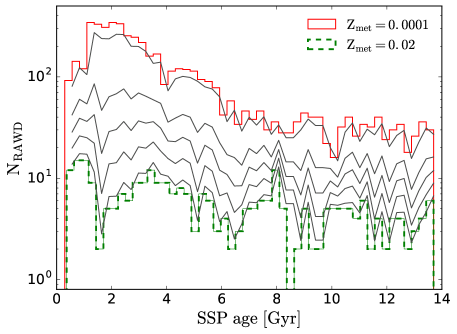
Figure 12: Same as in Figure 5 but only accounting for $Z=0.0001$ and 0.02. The grey lines are the linearly interpolated rates for the same metallicities as in RAWD yields (see Section 2). The interpolation has been made in the log-log space.

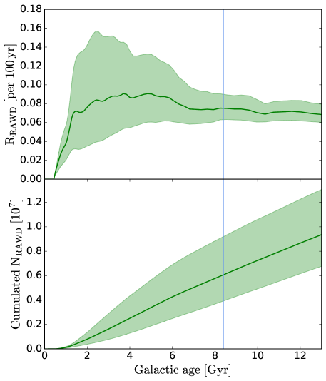
Figure 13: Same as in Figure 7, but using the RAWD rates shown in Figure 12.

Table 3: Same as in Table 2, but using the RAWD rates shown in Figure 12.

Z	Element	RAWDs contribution [%]
		Fiducial (L09)	GCE (L09)	Nucl. React. (L09)	Combined (L09)	Combined (A09)
35	Br	3.4	[ 1.3 - 8.1]	—	[ 1.3 - 8.1]	—
36	Kr	8.3	[ 3.3 - 19.5 ]	—	[ 3.3 - 19.5 ]	[ 3.5 - 20.9 ]
37	Rb	24.0	[ 9.5 - 55.8 ]	[ 15.2 - 38.0 ]	[ 6.0 - 88.3 ]	[ 4.3 - 63.9 ]
38	Sr	5.6	[ 2.3 - 12.8 ]	[ 3.26 - 9.7 ]	[ 1.3 - 22.1 ]	[ 1.4 - 23.6 ]
39	Y	11.2	[ 4.6 - 26.3 ]	[ 5.7 - 22.3 ]	[ 2.3 - 52.2 ]	[ 2.2 - 51.0 ]
40	Zr	11.0	[ 4.6 - 26.1 ]	[ 6.3 - 19.0 ]	[ 2.6 - 45.3 ]	[ 2.6 - 44.2 ]
41	Nb	8.0	[ 3.3 - 18.9 ]	[ 2.1 - 30.4 ]	[ 0.9 - 72.1 ]	[ 0.8 - 65.8 ]
42	Mo	11.4	[ 4.9 - 27.3 ]	[ 4.7 - 27.5 ]	[ 2.0 - 65.8 ]	[ 2.3 - 75.5 ]
44	Ru	2.4	[ 1.1 - 5.6 ]	[ 0.9 - 6.0 ]	[ 0.4 - 14.2 ]	[ 0.5 - 15.2 ]

References

- Arcones & Thielemann (2013) Arcones, A., & Thielemann, F.-K. 2013, Journal of Physics G Nuclear Physics, 40, 013201
- Asplund et al. (2009) Asplund, M., Grevesse, N., Sauval, A. J., & Scott, P. 2009, ARA&A, 47, 481
- Asplund et al. (1999) Asplund, M., Lambert, D. L., Kipper, T., Pollacco, D., & Shetrone, M. D. 1999, A&A, 343, 507
- Battino et al. (2016) Battino, U., Pignatari, M., Ritter, C., et al. 2016, ApJ, 827, 30
- Belczynski et al. (2002) Belczynski, K., Kalogera, V., & Bulik, T. 2002, ApJ, 572, 407
- Belczynski et al. (2008) Belczynski, K., Kalogera, V., Rasio, F. A., et al. 2008, ApJS, 174, 223
- Bensby et al. (2014) Bensby, T., Feltzing, S., & Oey, M. S. 2014, A&A, 562, A71
- Bisterzo et al. (2014) Bisterzo, S., Travaglio, C., Gallino, R., Wiescher, M., & Käppeler, F. 2014, ApJ, 787, 10
- Botyánszki et al. (2018) Botyánszki, J., Kasen, D., & Plewa, T. 2018, ApJ, 852, L6
- Bours et al. (2013) Bours, M. C. P., Toonen, S., & Nelemans, G. 2013, A&A, 552, A24
- Cassisi et al. (1998) Cassisi, S., Iben, I. J., & Tornambé, A. 1998, ApJ, 496, 376
- Chen et al. (2014) Chen, H.-L., Woods, T. E., Yungelson, L. R., Gilfanov, M., & Han, Z. 2014, MNRAS, 445, 1912
- Chiappini et al. (1997) Chiappini, C., Matteucci, F., & Gratton, R. 1997, ApJ, 477, 765
- Chiappini et al. (2001) Chiappini, C., Matteucci, F., & Romano, D. 2001, ApJ, 554, 1044
- Chieffi & Limongi (2004) Chieffi, A., & Limongi, M. 2004, ApJ, 608, 405
- Ciaraldi-Schoolmann et al. (2013) Ciaraldi-Schoolmann, F., Seitenzahl, I. R., & Röpke, F. K. 2013, A&A, 559, A117
- Clarkson et al. (2017) Clarkson, O., Herwig, F., & Pignatari, M. 2017, ArXiv e-prints, arXiv:1710.01763 [astro-ph.SR]
- Connelly et al. (2017) Connelly, J. N., Bollard, J., & Bizzarro, M. 2017, Geochim. Cosmochim. Acta, 201, 345
- Côté et al. (2017a) Côté, B., O’Shea, B. W., Ritter, C., Herwig, F., & Venn, K. A. 2017a, ApJ, 835, 128
- Côté et al. (2017b) Côté, B., Silvia, D., O’Shea, B. W., Smith, B., & Wise, J. H. 2017b, ArXiv e-prints, arXiv:1710.06442
- Côté et al. (2016) Côté, B., West, C., Heger, A., et al. 2016, MNRAS, 463, 3755
- Cowan & Rose (1977) Cowan, J. J., & Rose, W. K. 1977, ApJ, 212, 149
- Cristallo et al. (2015a) Cristallo, S., Abia, C., Straniero, O., & Piersanti, L. 2015a, ApJ, 801, 53
- Cristallo et al. (2015b) Cristallo, S., Straniero, O., Piersanti, L., & Gobrecht, D. 2015b, ApJS, 219, 40
- Denissenkov et al. (2016) Denissenkov, P., Perdikakis, G., Herwig, F., et al. 2016, ArXiv e-prints, arXiv:1611.01121 [astro-ph.SR]
- Denissenkov et al. (2017) Denissenkov, P. A., Herwig, F., Battino, U., et al. 2017, ApJ, 834, L10
- Dominik et al. (2012) Dominik, M., Belczynski, K., Fryer, C., et al. 2012, ApJ, 759, 52
- Duquennoy & Mayor (1991) Duquennoy, A., & Mayor, M. 1991, A&A, 248, 485
- Fenner & Gibson (2003) Fenner, Y., & Gibson, B. K. 2003, PASA, 20, 189
- Ferrini et al. (1992) Ferrini, F., Matteucci, F., Pardi, C., & Penco, U. 1992, ApJ, 387, 138
- Fisher & Jumper (2015) Fisher, R., & Jumper, K. 2015, ApJ, 805, 150
- Frischknecht et al. (2016) Frischknecht, U., Hirschi, R., Pignatari, M., et al. 2016, MNRAS, 456, 1803
- Fröhlich et al. (2006) Fröhlich, C., Martínez-Pinedo, G., Liebendörfer, M., et al. 2006, Physical Review Letters, 96, 142502
- Gallino et al. (1998) Gallino, R., Arlandini, C., Busso, M., et al. 1998, ApJ, 497, 388
- Gibson et al. (2003) Gibson, B. K., Fenner, Y., Renda, A., Kawata, D., & Lee, H.-c. 2003, PASA, 20, 401
- Hampel et al. (2016) Hampel, M., Stancliffe, R. J., Lugaro, M., & Meyer, B. S. 2016, ApJ, 831, 171
- Han & Podsiadlowski (2004) Han, Z., & Podsiadlowski, P. 2004, MNRAS, 350, 1301
- Heger & Woosley (2010) Heger, A., & Woosley, S. E. 2010, ApJ, 724, 341
- Heil et al. (2007) Heil, M., Käppeler, F., Uberseder, E., Gallino, R., & Pignatari, M. 2007, Progress in Particle and Nuclear Physics, 59, 174
- Heringer et al. (2017) Heringer, E., Pritchet, C., Kezwer, J., et al. 2017, ApJ, 834, 15
- Herwig (2001) Herwig, F. 2001, Ap&SS, 275, 15
- Herwig (2005) —. 2005, ARA&A, 43, 435
- Herwig et al. (2007) Herwig, F., Freytag, B., Fuchs, T., et al. 2007, in Astronomical Society of the Pacific Conference Series, Vol. 378, Why Galaxies Care About AGB Stars: Their Importance as Actors and Probes, ed. F. Kerschbaum, C. Charbonnel, & R. F. Wing, 43
- Herwig et al. (2011) Herwig, F., Pignatari, M., Woodward, P. R., et al. 2011, ApJ, 727, 89
- Hirai et al. (2015) Hirai, Y., Ishimaru, Y., Saitoh, T. R., et al. 2015, ApJ, 814, 41
- Hirai et al. (2017) —. 2017, MNRAS, 466, 2474
- Hitomi Collaboration (2017) Hitomi Collaboration. 2017, Nature, 551, 478
- Hoffman et al. (2001) Hoffman, R. D., Woosley, S. E., & Weaver, T. A. 2001, ApJ, 549, 1085
- Ivanova et al. (2013) Ivanova, N., Justham, S., Chen, X., et al. 2013, A&A Rev., 21, 59
- Iwamoto et al. (1999) Iwamoto, K., Brachwitz, F., Nomoto, K., et al. 1999, ApJS, 125, 439
- Johansson et al. (2014) Johansson, J., Woods, T. E., Gilfanov, M., et al. 2014, MNRAS, 442, 1079
- Johansson et al. (2016) —. 2016, MNRAS, 461, 4505
- Just et al. (2015) Just, O., Bauswein, A., Pulpillo, R. A., Goriely, S., & Janka, H.-T. 2015, MNRAS, 448, 541
- Karakas & Lattanzio (2014) Karakas, A. I., & Lattanzio, J. C. 2014, PASA, 31, e030
- Karakas & Lugaro (2016) Karakas, A. I., & Lugaro, M. 2016, ApJ, 825, 26
- Kobayashi et al. (2006) Kobayashi, C., Umeda, H., Nomoto, K., Tominaga, N., & Ohkubo, T. 2006, ApJ, 653, 1145
- Kromer et al. (2015) Kromer, M., Ohlmann, S. T., Pakmor, R., et al. 2015, MNRAS, 450, 3045
- Kroupa (2001) Kroupa, P. 2001, MNRAS, 322, 231
- Kroupa et al. (1993) Kroupa, P., Tout, C. A., & Gilmore, G. 1993, MNRAS, 262, 545
- Kubryk et al. (2015) Kubryk, M., Prantzos, N., & Athanassoula, E. 2015, A&A, 580, A126
- Lepo & van Kerkwijk (2013) Lepo, K., & van Kerkwijk, M. 2013, ApJ, 771, 13
- Li et al. (2011) Li, W., Chornock, R., Leaman, J., et al. 2011, MNRAS, 412, 1473
- Lodders et al. (2009) Lodders, K., Palme, H., & Gail, H.-P. 2009, Landolt Börnstein, arXiv:0901.1149 [astro-ph.EP]
- Lugaro et al. (2003) Lugaro, M., Herwig, F., Lattanzio, J. C., Gallino, R., & Straniero, O. 2003, ApJ, 586, 1305
- Lugaro et al. (2014) Lugaro, M., Tagliente, G., Karakas, A. I., et al. 2014, ApJ, 780, 95
- Ma et al. (2013) Ma, X., Chen, X., Chen, H.-l., Denissenkov, P. A., & Han, Z. 2013, ApJ, 778, L32
- Maguire et al. (2016) Maguire, K., Taubenberger, S., Sullivan, M., & Mazzali, P. A. 2016, MNRAS, 457, 3254
- Malaney (1986) Malaney, R. A. 1986, MNRAS, 223, 683
- Mannucci et al. (2005) Mannucci, F., Della Valle, M., Panagia, N., et al. 2005, A&A, 433, 807
- Martin et al. (2016) Martin, D., Arcones, A., Nazarewicz, W., & Olsen, E. 2016, Physical Review Letters, 116, 121101
- Martin et al. (2015) Martin, D., Perego, A., Arcones, A., et al. 2015, ApJ, 813, 2
- Martínez-Pinedo et al. (2014) Martínez-Pinedo, G., Fischer, T., & Huther, L. 2014, Journal of Physics G Nuclear Physics, 41, 044008
- Matteucci & Greggio (1986) Matteucci, F., & Greggio, L. 1986, A&A, 154, 279
- McWilliam et al. (2017) McWilliam, A., Piro, A. L., Badenes, C., & Bravo, E. 2017, ArXiv e-prints, arXiv:1710.05030 [astro-ph.HE]
- Moe & Di Stefano (2017) Moe, M., & Di Stefano, R. 2017, ApJS, 230, 15
- Montes et al. (2007) Montes, F., Beers, T. C., Cowan, J., et al. 2007, ApJ, 671, 1685
- Mumpower et al. (2016) Mumpower, M. R., Surman, R., McLaughlin, G. C., & Aprahamian, A. 2016, Progress in Particle and Nuclear Physics, 86, 86
- Nishimura et al. (2012) Nishimura, N., Fischer, T., Thielemann, F.-K., et al. 2012, ApJ, 758, 9
- Nomoto et al. (2013) Nomoto, K., Kobayashi, C., & Tominaga, N. 2013, ARA&A, 51, 457
- Nomoto et al. (2007) Nomoto, K., Saio, H., Kato, M., & Hachisu, I. 2007, ApJ, 663, 1269
- Pakmor et al. (2012) Pakmor, R., Kromer, M., Taubenberger, S., et al. 2012, ApJ, 747, L10
- Pardi et al. (1995) Pardi, M. C., Ferrini, F., & Matteucci, F. 1995, ApJ, 444, 207
- Paxton et al. (2013) Paxton, B., Cantiello, M., Arras, P., et al. 2013, ApJS, 208, 4
- Perego et al. (2014) Perego, A., Rosswog, S., Cabezón, R. M., et al. 2014, MNRAS, 443, 3134
- Philcox et al. (2017) Philcox, O., Rybizki, J., & Gutcke, T. 2017, ArXiv e-prints, arXiv:1712.05686
- Pignatari et al. (2010) Pignatari, M., Gallino, R., Heil, M., et al. 2010, ApJ, 710, 1557
- Pignatari et al. (2013) Pignatari, M., Hirschi, R., Wiescher, M., et al. 2013, ApJ, 762, 31
- Pignatari et al. (2016) Pignatari, M., Herwig, F., Hirschi, R., et al. 2016, ApJS, 225, 24
- Portinari et al. (1998) Portinari, L., Chiosi, C., & Bressan, A. 1998, A&A, 334, 505
- Postnov & Yungelson (2014) Postnov, K. A., & Yungelson, L. R. 2014, Living Reviews in Relativity, 17, 3
- Prantzos et al. (1990) Prantzos, N., Hashimoto, M., & Nomoto, K. 1990, A&A, 234, 211
- Raiteri et al. (1993) Raiteri, C. M., Gallino, R., Busso, M., Neuberger, D., & Kaeppeler, F. 1993, ApJ, 419, 207
- Ritter et al. (2017a) Ritter, C., Côté, B., Herwig, F., Navarro, J. F., & Fryer, C. 2017a, ArXiv e-prints, arXiv:1711.09172
- Ritter et al. (2017b) Ritter, C., Herwig, F., Jones, S., et al. 2017b, ArXiv e-prints, arXiv:1709.08677 [astro-ph.SR]
- Roederer et al. (2016) Roederer, I. U., Karakas, A. I., Pignatari, M., & Herwig, F. 2016, ApJ, 821, 37
- Ruiter et al. (2009) Ruiter, A. J., Belczynski, K., & Fryer, C. 2009, ApJ, 699, 2026
- Ruiter et al. (2011) Ruiter, A. J., Belczynski, K., Sim, S. A., et al. 2011, MNRAS, 417, 408
- Sato et al. (2016) Sato, Y., Nakasato, N., Tanikawa, A., et al. 2016, ApJ, 821, 67
- Seitenzahl et al. (2013) Seitenzahl, I. R., Cescutti, G., Röpke, F. K., Ruiter, A. J., & Pakmor, R. 2013, A&A, 559, L5
- Shappee et al. (2017) Shappee, B. J., Stanek, K. Z., Kochanek, C. S., & Garnavich, P. M. 2017, ApJ, 841, 48
- Shen et al. (2013) Shen, K. J., Guillochon, J., & Foley, R. J. 2013, ApJ, 770, L35
- Starkenburg et al. (2017) Starkenburg, E., Oman, K. A., Navarro, J. F., et al. 2017, MNRAS, 465, 2212
- Stritzinger et al. (2015) Stritzinger, M. D., Valenti, S., Hoeflich, P., et al. 2015, A&A, 573, A2
- Talbot & Arnett (1971) Talbot, Jr., R. J., & Arnett, W. D. 1971, ApJ, 170, 409
- Tinsley (1979) Tinsley, B. M. 1979, ApJ, 229, 1046
- Toonen et al. (2014) Toonen, S., Claeys, J. S. W., Mennekens, N., & Ruiter, A. J. 2014, A&A, 562, A14
- Travaglio et al. (1999) Travaglio, C., Galli, D., Gallino, R., et al. 1999, ApJ, 521, 691
- Travaglio et al. (2004) Travaglio, C., Gallino, R., Arnone, E., et al. 2004, ApJ, 601, 864
- van den Heuvel et al. (1992) van den Heuvel, E. P. J., Bhattacharya, D., Nomoto, K., & Rappaport, S. A. 1992, A&A, 262, 97
- Van Der Walt et al. (2011) Van Der Walt, S., Colbert, S. C., & Varoquaux, G. 2011, ArXiv e-prints, arXiv:1102.1523 [cs.MS]
- van Rossum et al. (2016) van Rossum, D. R., Kashyap, R., Fisher, R., et al. 2016, ApJ, 827, 128
- Wanajo (2006) Wanajo, S. 2006, ApJ, 647, 1323
- Wanajo (2013) —. 2013, ApJ, 770, L22
- Wanajo et al. (2011) Wanajo, S., Janka, H.-T., & Müller, B. 2011, ApJ, 726, L15
- Webbink (1984) Webbink, R. F. 1984, ApJ, 277, 355
- Wheeler (2012) Wheeler, J. C. 2012, ApJ, 758, 123
- Wise et al. (2012) Wise, J. H., Turk, M. J., Norman, M. L., & Abel, T. 2012, ApJ, 745, 50
- Wolf et al. (2013) Wolf, W. M., Bildsten, L., Brooks, J., & Paxton, B. 2013, ApJ, 777, 136
- Woods et al. (2017) Woods, T. E., Ghavamian, P., Badenes, C., & Gilfanov, M. 2017, Nature Astronomy, 1, 263
- Woods & Gilfanov (2016) Woods, T. E., & Gilfanov, M. 2016, MNRAS, 455, 1770
- Yamaguchi et al. (2015) Yamaguchi, H., Badenes, C., Foster, A. R., et al. 2015, ApJ, 801, L31