Discrete energy estimates for the -systems††thanks: received on , and accepted date (The correct dates will be entered by the editor).
Abstract
In this article, we propose finite volume schemes for the -systems and we establish stability and error estimates. The order of accuracy depends on the so-called BBM-type dispersion coefficients and . If , the numerical schemes are accurate, while if , we obtain an -order of convergence. The analysis covers a broad range of the parameters . In the second part of the paper, numerical experiments validating the theoretical results as well as head-on collision of traveling waves are investigated.
keywords:
system ; numerical convergence; error estimates65M12; 35Q35
1 Introduction
Consider a layer of incompressible, irrotational, perfect fluid flowing through a channel with flat bottom represented by the plane:
with , the depth of the channel. We assume that the fluid at rest occupies all the region . We suppose also that the free surface resulting after a perturbation of the rest state can be described by the graph of some function. Let be the maximum amplitude of the wave and a typical wavelength. Furthermore, consider:
The Boussinesq regime
describes small amplitude, long wavelength water waves. In order to study waves that fit into the Boussinesq regime, Bona, Chen and Saut, [22], derived the so-called -systems:
| (1.1) |
with the identity operator. In the system (1.1), represents the deviation of the free surface from the rest position, while is the fluid velocity. The above family of systems is derived in [22] from the classical water waves problem by a formal series expansion and by neglecting the second and higher order terms. In fact, one may regard the zeros on the right hand side of (1.1) as the second order terms (i.e. having one of , or as a prefactor) neglected in the modeling process in order to establish (1.1). In [24], Bona, Colin and Lannes prove rigorously that the systems (1.1) approximate the water waves problem in the sense that the error estimate between the solution of (1.1) and the solution of the water waves system at time is of order (see also [27]).
The parameters are restricted by the following relation:
| (1.2) |
Nevertheless, if surface tension is taken into account then, the previous relation rewrites
where is the Bond number which characterizes the surface tension parameter, see [19] or [21].
In [12], models taking into account more general topographies of the bottom of the channel are obtained. One has to furthermore distinguish between two different regimes: small respectively strong topography variations. Time-changing bottom-topographies are considered in [14]. For a systematic study of approximate models for the water waves problem along with their rigorous justification, we refer the reader to the work of Lannes [27]. We point out that the only values of for which (1.1) is physically relevant are .
The systems are well-posed locally in time in the following cases:
| (1.3) | ||||
| (1.4) |
see for instance Bona, Chen and Saut [23], Anh [2] and Linares, Pilod and Saut [20]. Global existence is known to hold true in dimension for the ”classical” Boussinesq system:
which was studied by Amick in [1] and Schonbek in [31] and for the so-called Bona-Smith systems:
assuming some smallness condition on the initial data, see [23] and the work of Bona and Smith [8]. In the remaining cases, the problem is still open.
Lower bounds on the time of existence of solutions of systems (1.1) in terms of the physical parameters are obtained in [30], [21], [28], [10] for initial data lying in Sobolev classes, respectively in [9] for initial data manifesting nontrivial values at infinity.
In the following lines, let us recall some important numerical results obtained for the systems (1.1).
One of the earliest papers in this sense is the work of Peregrine [29], who numerically investigates undular bore propagation using the “classical” Boussinesq system corresponding to the values , .
In [6], Bona and Chen study the boundary value problem for the BBM-BBM case (which corresponds to ). Using an integral reformulation of this problem, they construct a numerical scheme, which is proven to be fourth order accurate in both time and space. They employ it in order to track down generalized solitary waves and to study the collision between this numerical generalized solitary waves.
In [25] and [26], Bona, Dougalis and Mitsotakis investigate the periodic value problem for the so-called KdV-KdV case, which corresponds to . They propose a numerical scheme constructed by using an implicit Runge-Kutta method for the time discretization and a Galerkin method with periodic splines scheme for the space discretization. They use this scheme in order to track down generalized solitary wave solutions and they simulate head-on collision of two such waves.
In [17], Antonopoulus, Dougalis and Mitsotakis study the periodic initial value problem for a large class of values of the parameters. More precisely, they obtain error estimates for semi-discretization schemes (in space) obtained via Galerkin approximation. In [18], the same authors obtain error estimates for a full-discretization scheme of the initial value problem with non-homogeneous Dirichlet and reflection boundary conditions for the Bona-Smith system (corresponding to the case , , ). They use their numerical algorithm to study soliton interactions.
In [4], (see also [3] for more details) Antonopoulos and Dougalis obtain error estimates for a semi-discrete and fully-discrete Galerkin-finite element scheme for the initial boundary value problems (ibvp) for the “classical” Boussinesq system.
Regarding the two dimensional case [33], Dougalis, Mitsotakis and Saut study a space semi-discretization scheme using a Galerkin method. In [15], Chen, using a formal second-order semi-implicit Crank-Nicolson scheme along with spectral method, studies the case of the BBM-BBM system for D water waves over an uneven bottom.
A very recent result of Bona and Chen [7] provides numerical evidence of finite time blow-up for the BBM-BBM system. The blow-up phenomena seems to occur on head-on collision of some particular traveling waves solutions of the BBM system.
1.1 Statement of the main results.
To the authors knowledge, fully-discretized schemes for various ibvp for -systems along with error estimates are available in only four cases :
In this paper, we implement fully-discrete finite volume schemes, and we prove convergence and stability estimates, using a discrete variant of the ”natural” energy functional associated to these systems. One practical advantage of our approach is that it allows us to treat explicitly the nonlinear terms.
Let us recall that the Cauchy problem associated with the one dimensional -systems reads:
| () |
We will treat the cases where the parameters verify:
| (1.5) |
excluding the five cases:
| (1.6) |
Remark 1.1.
The Shallow Water case corresponds to a classical non-symmetric hyperbolic system. A systematic method to construct appropriate semi-discrete schemes is presented in [32]. More recently, this case has been studied in [5]. The authors construct a finite-volume-Galerkin numerical scheme, where discrete estimates in are obtained.
Given , we will consider the following set of indices:
| (1.7) |
where the sign function is given by:
We will consider the set of indices defined by (1.7). The notation, stands for the space of continuous functions on with values in the space . Let us recall in the following lines, the existence result of regular solution that can be found for instance in [10] and [21]:
Theorem 1.2.
Consider and excluding the cases . Also, consider an integer such that
and , defined by (1.7). Let us consider . Then, there exists a positive time and a unique solution
Remark 1.3.
Note that energy is an energy for the system (), see for exemple [10],
Consider and two positive real numbers. We endow with the following scalar product and norm
We sometimes denote this space .
For all , we introduce the spatial shift operators:
If , we denote by the discrete derivation operators:
Also, we consider the following discrete energy functional
| (1.8) |
We will now discuss the main results of the paper. From an initial datum with large enough, there exists a solution of () which enables to define given by:
| (1.9) |
Moreover, we define
| (1.10) |
The results of the paper are gathered in two cases according to the values of the parameters and in ().
The case when and
The assumption assures an -control on the discrete derivatives: this makes it possible to implement an energy method that mimics the one from the continuous case. Moreover, it allows us to close the estimates even without considering numerical viscosity.
We consider the following numerical scheme:
| (1.11) |
for all and or , with the discrete initial datum
| (1.12) |
The convergence error is defined as:
| (1.13) |
Remark 1.4.
For the linear part of the system, when , we consider the Crank-Nicolson discretization whereas for , we consider the implicit discretization.
We are now in the position of stating our first result.
Theorem 1.5.
Let , and . Consider , and such that is the solution on of the system (). Let , there exists a positive constant depending on such that if the number of time steps and the space discretization step are chosen such that
if we consider the numerical scheme (1.11) with or along with the initial data (1.12) as well as the approximation , defined by (1.9)-(1.10), where , then, the numerical scheme (1.11) is first order convergent in time and second order convergent in space i.e. the convergence error defined in (1.13) satisfies:
| (1.14) |
where depends on the parameters ,,,, on and on .
Remark 1.6.
Note that no Courant-Friedrichs-Lewy-type condition (CFL-type condition hereafter) is needed. This is due to the regularity properties of the operators and which ensure stability even if a centered scheme is used to discretize the hyperbolic part of the system.
Remark 1.7.
If we consider the Cauchy problem with small parameter :
The previous scheme is transformed into
for all and or . The conditions on the time step and space discretization in Theorem 1.5 become then and and the energy inequality rewrites
which impose a strong restriction on and .
In order to avoid this inconvenience, one should design an asymptotic preserving scheme, for which the error estimates are uniform with respect to . In such a scheme, both limits and may be commuted without affecting the accuracy of the scheme. Moreover, in such a scheme, the limit scheme when is consistent with the limit continuous system when . In the case of the -systems, the limit system when is the acoustic wave system.
The case when
We consider the following numerical scheme:
| (1.15) |
for all , with
| (1.16) |
Remark 1.8.
For the case , we consider only an implicit time discretization for the linear part of the system.
The convergence error is defined by . We are now in the position of stating our second main result.
Theorem 1.9.
Let , and with , excluding the cases (1.6). Consider , and such that is the solution on of the system ().
Choose and such that:
There exists (depending on , and on ) such that if the number of time steps and the space discretization step are chosen in order to verify
and
| (1.17) |
if we consider the numerical scheme (1.15) along with the initial data (1.16) with the numerical viscosities and as well as the approximation defined by (1.9), then, the numerical scheme (1.15) is first order convergent i.e. the convergence error defined in (1.13) satisfies:
where depends on the parameters ,,,, on and on .
Remark 1.10.
In this case, one of the two equations of (1.15) does not contain the operator or . Artificial viscosity together with a hyperbolic CFL-type condition are thus needed in order to stabilize the numerical scheme. We use a centered scheme for the first-order derivatives combined with a Rusanov-type diffusion coefficient and a CFL-type condition (which, of course, corresponds to Relation (1.17)).
Remark 1.11.
In order to have less diffusive schemes, we may in fact update the Rusanov coefficient at each time step i.e. take depending on such that
Remark 1.12.
Our results owe much to the technics developed recently by Courtès, Lagoutière and Rousset in [11]. Let us give some more details. In order to study the Korteweg-de-Vries equation
they employ the following -scheme, with ,
With the aim to study the order of convergence, they consider the finite volume discrete operators:
and the convergence error
which obeys the following equation:
with
where is the consistency error. In order to establish -estimates, they show that under the CFL condition
the following holds true:
| (1.18) |
provided that is sufficiently small. Thus, they are able to use the discrete Gronwall lemma and close their estimates. The proof of is rather technical and tricky. Loosely speaking, using some clever identities when computing , they get several negative terms wich, under the above CFL and smallness conditions, are used to balance the ”bad” terms.
In Section 2.2.1 we study a discrete operator which appears in hyperbolic systems and we provide a bound for its -norm, the proof being essentially inspired from [11]. As a consequence, we establish a higher-order estimate which proves crucial in the analysis of some of the -systems. Among the systems in view, we distinguish three situations:
-
•
when , establishing energy estimates for the convergence error can be done by imitating the approach from the continuous case. The structure of the equations provides enough control such that we do not need to impose numerical viscosity or CFL-type conditions.
-
•
when at least one of the weakly dispersive operators does not appear, we have to work only with estimations established in Section 2.2.1 (see for instance the case , ) either
-
•
combine the technics of Section 2.2.1 with ”continuous-type” estimates like those established for the case (see for instance the case ).
In order to illustrate the theoretical order of convergence (see Theorem 1.5 and Theorem 1.9), we compare the numerical solutions computed with our schemes with the exact traveling wave solutions which were computed by Chen in [13] and by Bona and Chen in [6].
Finally, we use our results in order to study exact traveling waves interactions. Our experiments are inspired from [4], [17], [6] and [7]. We perform two such numerical experiments. Recently, in [7] Bona and Chen pointed out that finite time blow-up seems to occur at the head-on collision of the two exact solutions:
In order to build confidence in our codes, we repeat their experiment, in the same conditions and we show that we obtain roughly the same results. We observed that the BBM-BBM system is not the only one having traveling waves of the above form. In particular, we provide numerical evidence that a blow-up phenomenon might occur on the head-on collision of the traveling waves for the case when the parameters are , .
The plan of the rest of this paper is the following. In the next section, we give a list of the main notations and identities that we use all along in this manuscript. Section 2.1 is devoted to the proof of Theorem 1.5. The proof of Theorem 1.9 is more involved as we cannot treat in a uniformly manner all the cases when . First, we establish in Section 2.2.1 some estimates for discrete operators appearing in hyperbolic systems. The rest of Section 2.2 is dedicated to the proof corresponding to the different values of the parameters appearing in Theorem 1.9. Finally, in Sections 3 and 4, we present our numerical simulations.
1.2 Notations.
In the following we present the main notations that will be used throughout the rest of the paper. Let us fix . For all , we introduce the spatial shift operators:
For , we define the product operator:
Also, we denote by
We list below some basic formulas, whose proofs can be found in [11].
The following identities describe the derivation law of a product, for
| (1.19) | ||||
| (1.20) | ||||
| (1.21) |
We observe that we dispose of the following basic integration by parts rules, for :
| (1.22) | ||||
| (1.23) |
In particular, we see that, for :
and
More elaborate integration by parts identities are the following, for ,
| (1.24) |
respectively
| (1.25) |
When in the previous equation, some additional simplifications occur and one has
| (1.26) |
Also, it holds true that, for ,
| (1.27) |
| (1.28) |
and
| (1.29) |
Finally, for , we recall Lemma 5 of [11]
| (1.30) |
and Lemma 8 of [11]
| (1.31) |
In the following, we will frequently use the notations:
| (1.32) |
We end this section with the following discrete version of Gronwall’s lemma, a proof of which can be found in [16]:
Lemma 1.13.
Let be sequences of real numbers with for all which satisfies
for all . Then, for any , we have:
2 The proof of the main results
2.1 The proof of Theorem 1.5.
Let us recall the energy functional:
| (2.33) |
For all , we will consider the consistency error defined as:
| (2.34) |
Proposition 2.1.
Proof 2.2.
As we announced in the introduction, we will establish energy estimates
imitating the approach from the continuous case.
For the Crank-Nicolson case (). Using the notations introduced in and , we see that the
equations governing the convergence error are
the following:
| (2.36) |
Let and observe that by multiplying the first equation of (2.36) by , the second by and adding up the results, we find that
| (2.37) | |||
We begin by treating the left hand side of (2.37). Notice that
with any linear operator. With this in mind together with Relations (1.22) and (1.23), it gives,
| (2.38) |
Let us now focus on . We recall that
and we write that, thanks to Cauchy-Schwarz inequality (we recall that and )
By applied Young inequality, we recover the -norm of and .
| (2.39) |
Let us treat . Using , we first write
Proceeding in a similar fashion with the other terms we arrive, thanks to the Cauchy-Schwarz inequality, at (we recall that )
By Definition (1.32) of , one has
These together give
| (2.40) |
where and can be written, for example, as a numerical constants multiplied with:
| (2.41) |
We treat in same spirit as above in order to obtain that
| (2.42) |
where and are multiples of :
| (2.43) |
In order to treat , we first observe that
Thus, we obtain
| (2.44) |
where respectively are proportional with
| (2.45) |
The same holds for , namely, we get that
| (2.46) |
where respectively are proportional with
| (2.47) |
Gathering the informations from , (2.38), , , , and we obtain the existence of two constants and that depend on and the -norm of and (dependence which we can track using relations , , respectively ) and that are proportional to such that
For the implicit case (). The equations governing the convergence error are the following
| (2.48) |
For that case, we fix the discret energy
| (2.49) |
This energy is of course equivalent to the one from (2.33).
Let us multiply the first equation of (2.48) by and the second one of (2.48) by . The sum of -norm gives in that case
| (2.50) |
The left hand side of the previous equality gives
For both cross products, it gives
Thanks to integration by parts, Young’s inequality together with Cauchy-Schwarz inequality, the previous equality simplifies into
The left hand side of (2.50) becomes
Due to the definition of the energy (2.49), one has
| (2.51) |
with
Let us now focus on the right hand side of (2.50). The triangular inequality together with Young’s inequality give the existence of a constant independent of , such that
Since
it holds
| (2.52) |
The same holds for other terms to obtain
| (2.53) |
and
| (2.54) |
and
| (2.55) |
and finally
| (2.56) |
Proof 2.3.
(Proof of Theorem 1.5.) Let us arbitrary fix . Suppose the strong induction hypothesis
| (2.58) |
for all .
This is obviously true for , since , for all . Let us prove that and .
Inequality (2.35) is thus available for any and constants and may be upper bounded by and independent of and
One has, for all
Namely, it becomes
Thus, taking the sum of all these inequalities, and noticing that , we end up with
Applying the discrete Grönwall lemma 1.13 and using the fact that the consistency error is first-order accurate in time and second-order accurate in space, see Appendix A, we get
where is some constant depending on the initial data . Thus, for small enough and using the inequality:
with a constant, we get that for sufficient small and :
We can assure that the inductive hypothesis holds for all .
Obviously, this allows to close the estimates and provide the desired bound. This concludes the proof of Theorem 1.5.
2.2 The proof of Theorem 1.9.
As announced in the introduction, in this section, we aim at providing a proof for our second main result. As opposed to the previous result, the proof of Theorem 1.9 is rather sensitive to the different values of the parameters.
We recall that we will treat the case where the parameters verify:
excluding the five cases:
For all , we will consider the consistency error defined as:
| (2.59) |
In this section, we only detail the derivation of the energy inequality for , the equivalent of (2.35). This inequality is summarized as follows.
Proposition 2.4.
Assume , with , for all . Then the following energy estimate holds true, for
| (2.60) |
with a positive constant depending on , and .
In order to close the estimates and ensure the convergence proof (as the one made in Subsection 2.1, for the case and ) we perform as usual an induction hypothesis on the smallness of according to the cases. It is sufficient to assume by induction
| (2.61) |
Hypothesis (2.61) is sufficient to assure the hypothesis of Proposition 2.4. The energy estimate (2.60) is thus satisfied and the convergence rate (Theorem 1.9) is a consequence of the discrete strong Grönwall inequality, Lemma 1.13 and the study of the consistency error (2.59) detailed in Appendix A (all the previous guidelines are detailed in Subsection 2.1 for the case and ).
First, we establish a technical result that interfers in a crucial manner in establishing the a priori estimates.
2.2.1 Burgers-type estimates.
Let us state the first result of this subsection:
Proposition 2.5.
Let such that and . Fix and such that
Then, there exists a sufficiently small positive number such that the following holds true. Consider two positive reals such that
and , such that
Then, there exists a positive constant depending on the -norm of and such that
Proof 2.6.
We define
We compute the -norm of :
| (2.62) |
For , Relations (1.24), (1.27) and (1.22) give
For the -term, one has, thanks to Relations
(1.31) and (1.25),
Eventually, for , one has, thanks to (1.26)
For the left hand side of the -norm of , Equation (2.62), we know, thanks to (1.30)
Thanks to (1.29), one has
and, thanks to (1.28),
Finally, we gather all these results
Thus
where
However,
By hypothesis, and , thus for such that
| (2.63) |
one has
This implies
In the same way, for and small enough and small enough, for satisfying
| (2.64) |
The next result is an immediate consequence of the preceding one.
Proposition 2.7.
Consider such that and . Fix such that
Then, there exist two sufficiently small positive numbers such that the following holds true. Consider two positive reals such that
and , such that
Then, there exists a positive constant depending on the -norm of and such that:
| (2.65) |
Proof 2.8.
Let us consider . Let us suppose that is chosen small enough such that
Then, taking a smaller and if neccesary, we may apply Proposition 2.5 with instead of in order to establish the estimate .
Proposition 2.9.
Consider such that and . Fix such that
Then, there exist two sufficiently small positive numbers such that the following holds true. Consider two positive reals such that
and , such that
| (2.66) | |||
| (2.67) |
Then, there exist positive constants , depending on the -norm of and such that:
Proof 2.10.
Let us observe that
Owing to the hypothesis - and Proposition 2.7 with instead of and instead of , we may choose small enough which ensures the existence of a positive constant such that:
| (2.68) |
Moreover, using the derivation formula (1.20), it transpires that
| (2.69) |
The conclusion follows from estimates and .
2.2.2 The case .
We distinguish many different settings for and .
The case , . The convergence error satisfies:
| (2.70) |
with
We consider the energy functional
Proof 2.11.
(Proof of Proposition 2.4 in the case , ). In order to recover a -type control for (necessary for the control of ), let us apply to the second equation of (2.70). We get that:
| (2.71) |
We consider now the three equations system comprised of system (2.70) with added equation (2.71). As previously, we square the equations and add them together. Young’s inequality enables us to obtain, with a constant
| (2.72) |
Let us consider the right hand side of (2.72). Owing to Proposition (2.7) and Proposition (2.5) we have that, thanks hypotheses of Proposition 2.4 on
| (2.73) |
respectively
| (2.74) |
Proposition 2.9 ensures the existence of constants such that:
| (2.75) |
Finally, we have, thanks Relation (1.20),
| (2.76) |
Eventually, we get, for the left hand side,
| (2.77) | |||
| (2.78) | |||
| (2.79) |
Gathering relations , , , , and (2.79) yields
2.2.3 The case .
Three configurations are studied in this subsubsection.
The case . In this case, without any difficulties, we are able to prove a more general
result. Indeed, we will show that the following general -scheme:
| (2.80) |
is adapted for studying the classical Boussinesq system, with . The convergence error verifies:
| (2.81) |
Recall that in this case:
| (2.82) |
Proof 2.12.
(Proof of Proposition 2.4 in the case ). Multiply the second equation of with and proceeding as we did in Section 2.1 (Identity (2.46) with ), we obtain that there exist two constants and depending on , , and , such that:
| (2.83) | |||
Notice that Relation (1.22) combined with the Cauchy-Schwarz inequality, the Young’s inequality and the upper bound simplifies the previous last term
A similar inequality holds true for .
Next, we rewrite the first equation of as
Thus, using the Proposition and Relation (1.20), we get that
| (2.84) |
with and depending on and . From , we deduce that
| (2.85) |
Adding up the estimates yields
The case . In this case, the convergence error satisfies:
In this section, we will work with the energy functional:
which is better adapted to the system corresponding to the particular values of the parameters in view here. Of course, is equivalent to the energy from .
Proof 2.13.
(Proof of Proposition 2.4 in the case ). By summing up the square of the -norm of the first equation by , the square of the norm of the second one by , we get that, thanks to Relations (1.22) and (1.23),
We notice that
Using Proposition 2.7 we get that
Also, we have, due to (1.20)
Proceeding as above, we get that:
Adding up the above estimate gives us:
The case . In this case, the convergence error satisfies:
| (2.86) |
Again, in order to close the estimates and prove the convergence of the scheme, we will be using the following energy functional:
which is equivalent to that one from .
Proof 2.14.
(Proof of Proposition 2.4 in the case ). In order to derive a -control on , let us apply in the first equation, to obtain
| (2.87) |
We focus now on the system composed of both equations of (2.86) with Equation (2.87) in addition. We will multiply the first and second equations of (2.86) by thereafter. As before, we square the three equalities to compute the -norm. Let us observe that
| (2.88) |
along with
| (2.89) |
and
| (2.90) |
Observe that the last term from cancels with the last term of , according to Relations (1.22) and (1.23). The same is true for in (2.88) and in (2.90). Therefore, by integrating by part in (2.88) and in (2.90), it yieds
Young’s inequality enables to lower bound the previous inequality:
Let us now focus on the right hand side of the squared equations. Using Cauchy-Schwarz inequality and Proposition 2.7, we get that
| (2.91) |
Using Proposition 2.9 and Young’s inequality, we get
| (2.92) | |||
| (2.93) |
Using once again the Young’s inequality, it holds
| (2.94) |
From - , we obtain
2.2.4 The case .
Once again, three configurations are considered according to the parameters and .
The case . In this case, as for the classical Boussinesq system (the case , page 2.2.3) we derive estimates for a
more general scheme: the following -scheme where the advection term is discretized according to a convex combination of and
| (2.95) |
The convergence error verifies:
| (2.96) |
We work with
| (2.97) |
Proof 2.15.
(Proof of Proposition 2.4 in the case ). We multiply the first equation by in order to get
Integration by parts (1.22) gives
| (2.98) |
with and two constants proportional to
Using the second equation of , the triangle inequality along with Proposition 2.5, one obtains:
| (2.99) |
Thus, by adding up estimate with the square of the estimate , we get that
The case . The convergence error satisfies:
| (2.100) |
Consider the energy functional we will work with will be
Proof 2.16.
(Proof of Proposition 2.4 in the case ). Let us multiply the first equation of (2.100) with to obtain:
| (2.101) |
The last inequality is due to Cauchy-Schwarz and Young’s inequalities. Notice that
with proportional to
Thus, Equation (2.101) becomes
| (2.102) |
Next, taking the square of the -norm of the second equation of and using Proposition 2.7, we obtain
| (2.103) |
When we will sum up Equations (2.102) and (2.103), both terms
will cancel each other, thanks to Relation (1.22). We have to cancel in (2.102) too. This is the aim of the following computation.
Applying into the second equation of and taking the square of the -norm of the
resulting equation yields (with Proposition 2.9)
| (2.104) |
Adding up the estimates , and leads to
The case . Finally, in this case, the convergence error satisfies:
| (2.105) |
In this case, we will use the energy functional:
Proof 2.17.
(Proof of Proposition 2.4 in the case ). Taking the square of the first equations of and multiplying the result with yields
| (2.106) |
Taking the square of the -norm of the second equation of leads to
| (2.107) |
Let us observe that the terms
and
can be lower controlled by the energy (by using integration by parts (1.22) and Cauchy-Schwarz inequality) such that they do not raise any issues. In order to get rid of the term
| (2.108) |
we will apply into the second equation of and consider the square of the -norm of the result. First, let us compute:
| (2.109) |
Of course the problematic term from will cancel with
appearing in . The additional term in (2.109) can be once again controlled by the energy (by using integrations by parts (1.22) and Cauchy-Schwarz inequality).
Let us now interest to the right hand side. For the first equation of , we obtain by Young inequality
| (2.110) |
In the previous inequality, we have upper bounded by
The second equation of gives
| (2.111) |
3 Experimental results
In order to illustrate our theoretical results, we compare in this paragraph, known exact
solutions (i.e. traveling waves) with the discrete solutions computed with the numerical schemes. We fix the space domain with . Moreover, we use periodic boundary conditions. Those conditions are not absorbing boundary
conditions, which would mimic perfectly the behavior on , but we fix the final time small enough and we take the initial
conditions localized enough in order to minimize boundary effects.
In Figures 2-10, we plot the exact and the numerical solutions which are computed with a space cell size and the time step .
The convergence results are gathered in Tables 1-5. The computations are performed with a number of cells for the values
The time step is chosen to be in order to verify the CFL-type condition. We perform computations up to the final time or . In the case where , we chose the Rusanov coefficients verifying and , when they are needed.
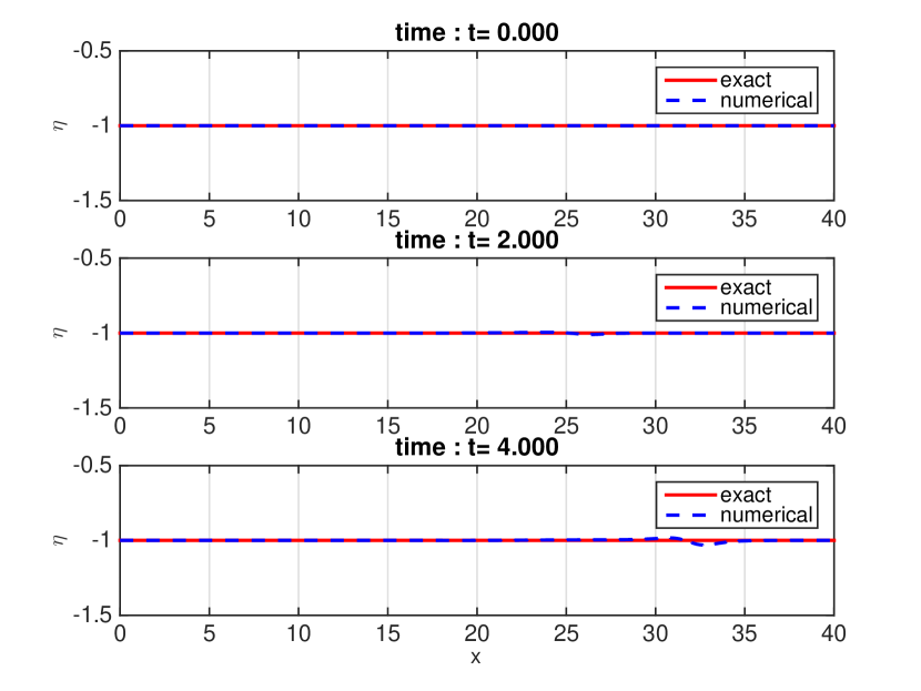
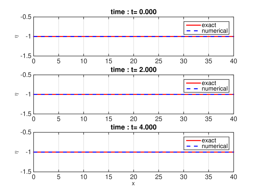
3.1 Linear case.
We begin by a test for the linear case:
| () |
More precisely, we take , , and and initialize the scheme with the initial datum
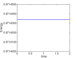
In this case, the discrete energy must be conserved if we use the Crank-Nicolson scheme (i.e. ). We perform computation up to the final time with space and time steps and with . The conclusion is that the discrete energy is conserved, more or less up to a factor of order , as it is illustrated by Figure 1.
3.2 Case , .
This section is divided in two parts. In the first part, we will illustrate experimentally the rates of accuracy obtained in Theorem 1.5. In the second part, we investigate in details the traveling-wave solutions.
Numerical convergence rates
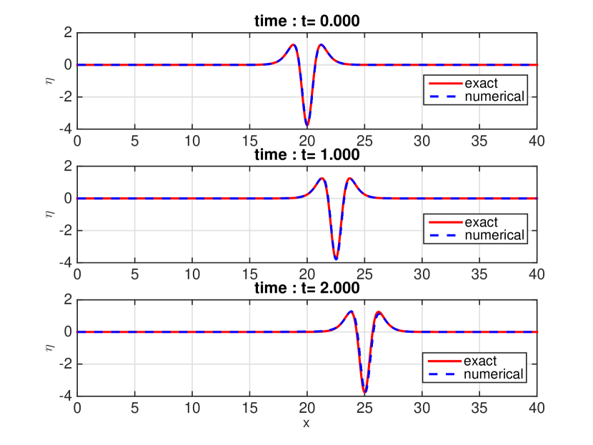
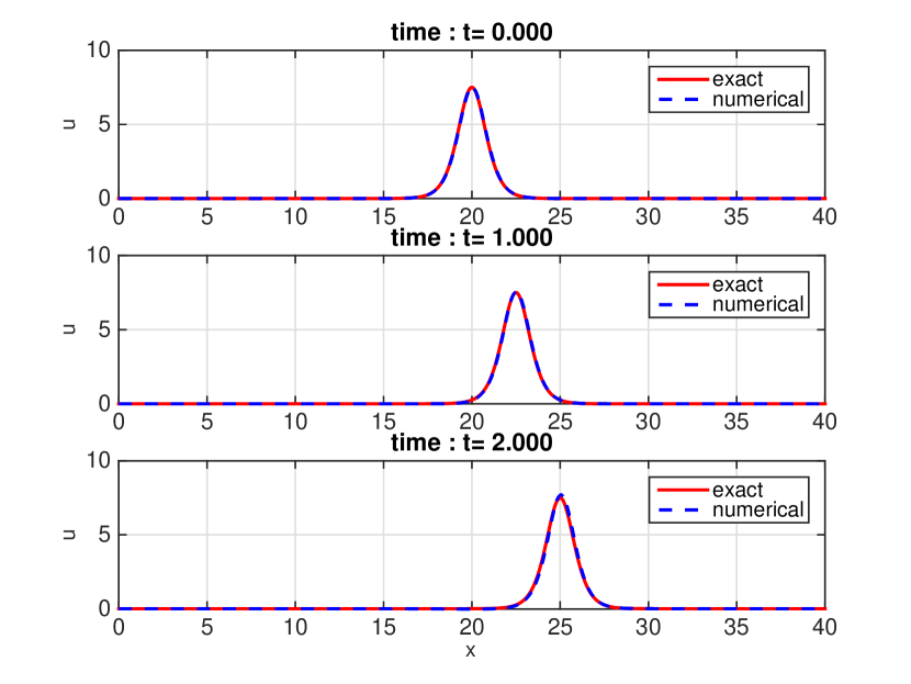
We first take a look at the BBM-BBM system with , , , for which two different exact solutions are known, see [6] and[13]. We perform a first experiment for the following family of exact solutions:
The results are represented in Figure 2.
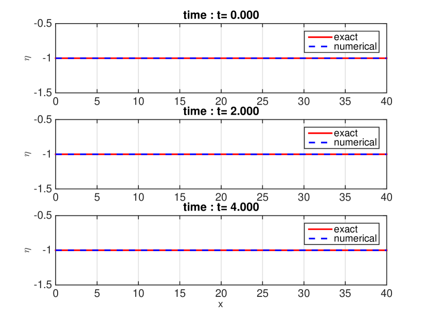
We perform a second experiment for the following family of solutions:
with and . The corresponding result can be found in Figure 3.
In order to compute a numerical rate of convergence, we perform computations with increasingly smaller space meshes. The results are gathered in Table 1.
| Case | Case | |||
| energy error | exp. rate | energy error | exp. rate | |
A third example that we treat concerns the case when , , and which is discussed in [13] for which the exact solution reads:
| Case | ||
| energy error | exp. rate | |
The fourth and last example that we present in this paragraph is the case when , , and , for which the exact solution writes:
We take and in order to perform our computations. The results are gathered in Figure 5 and Table 3.
| Case | ||
| energy error | exp. rate | |
Remark 3.1.
In these four examples, our numerical schemes do no contain artificial viscosity i.e. and . As we explained in the introduction, the parameters enable us to control and stabilize the scheme as the results of Figures 2-5 show.
The schemes used to perform these experiments are accurate so, if we take , we should be able to observe a second order convergence rate. The results when performing the above experiments with are gathered in Table 4 and confirm our intuition.
| Case | Case | |||
| energy error | exp. rate | energy error | exp. rate | |
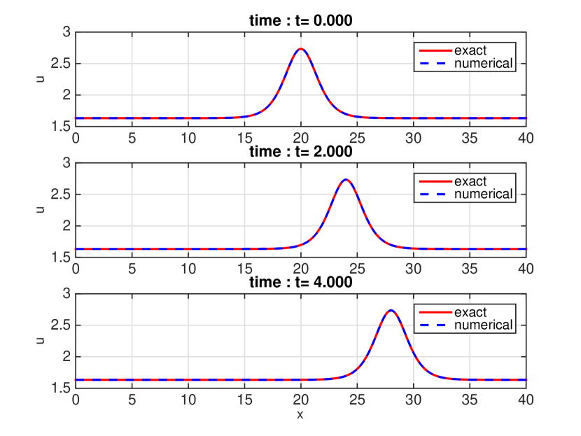
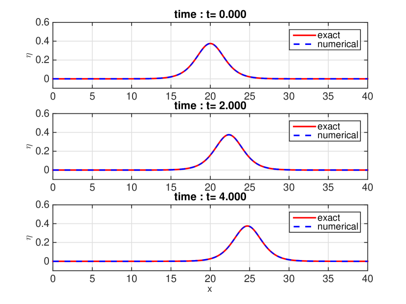
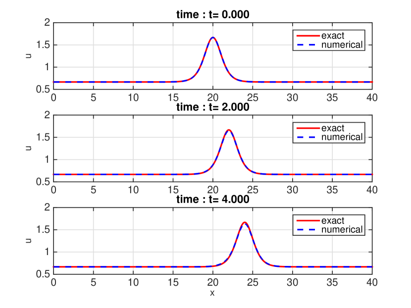
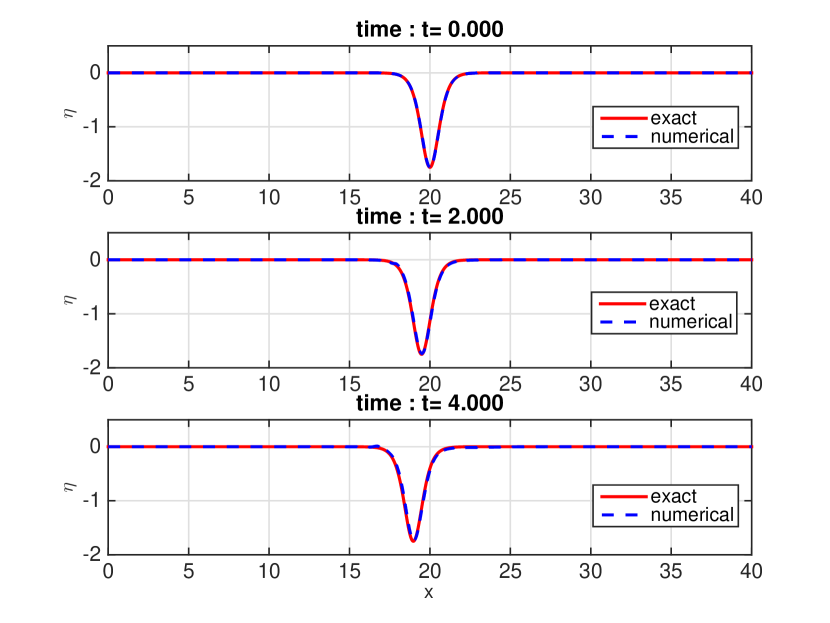
Behavior of the numerical scheme for traveling wave solutions
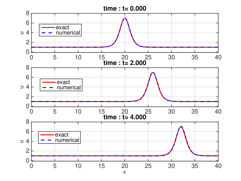
All the test cases studied previously are in fact traveling wave solutions and it is worth pushing forward our analysis for such particular solutions with the numerical schemes. First of all, since , the Rusanov coefficients and are taken equal to 0, which restricts the numerical diffusion of the scheme and provides a relatively good numerical solution in long temporal intervals, as seen in Figures 6 and 7. For test case , we have chosen and a space domain , whereas for test case , we have chosen and . In both simulations, the changes in amplitude are limited : the relative error on the maximum amplitude of is equal to at for the case and at for the case .
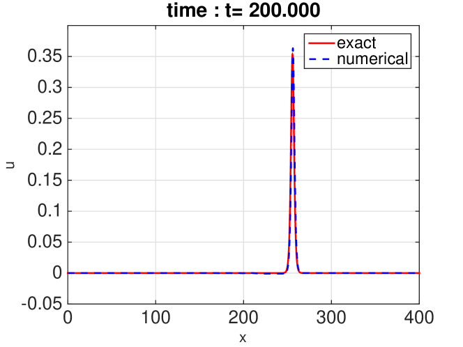
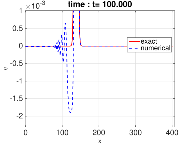
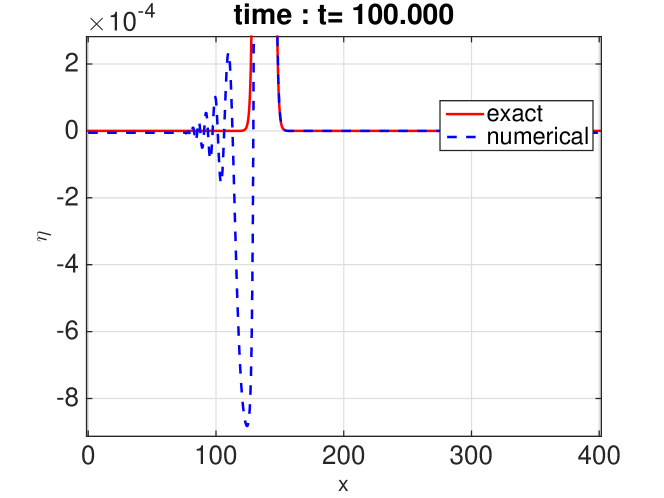
The oscillatory dispersive tails which may be visible in a zoom after the solitary wave are a numerical artifact. Thinner is the space mesh grid , smaller is the amplitude of these oscillations. For instance, the amplitude of this tail is divided by approximately 2.15 when is halved, see Figure 8.
3.3 Case .
We perform the same kind of numerical simulations : on the one hand, the validation of the convergence rates and on the other hand the behavior of the numerical schemes.
Numerical convergence rates
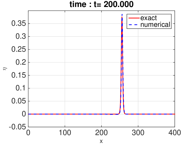
In the following two examples, we have chosen while . First, we consider the case when , . The exact solution obtained in [13] writes:
Our computations are done with and . We represent the numerical and the exact solutions in Figure 9.
In the second example, we treat the case , and , for which the exact solution obtained in [13] is:
We obtain Figure 10.
The experimental rates of convergence of the two previous cases with are gathered in Table 5
| Case | Case | |||
| energy error | exp. rate | energy error | exp. rate | |
Observe that the first order convergence is recovered which, of course, is in accordance with the theoretical results.
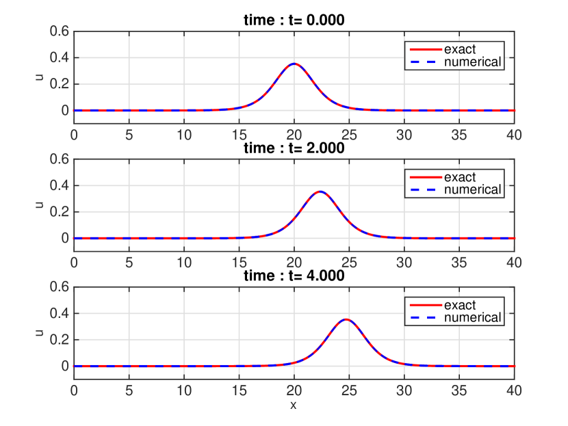
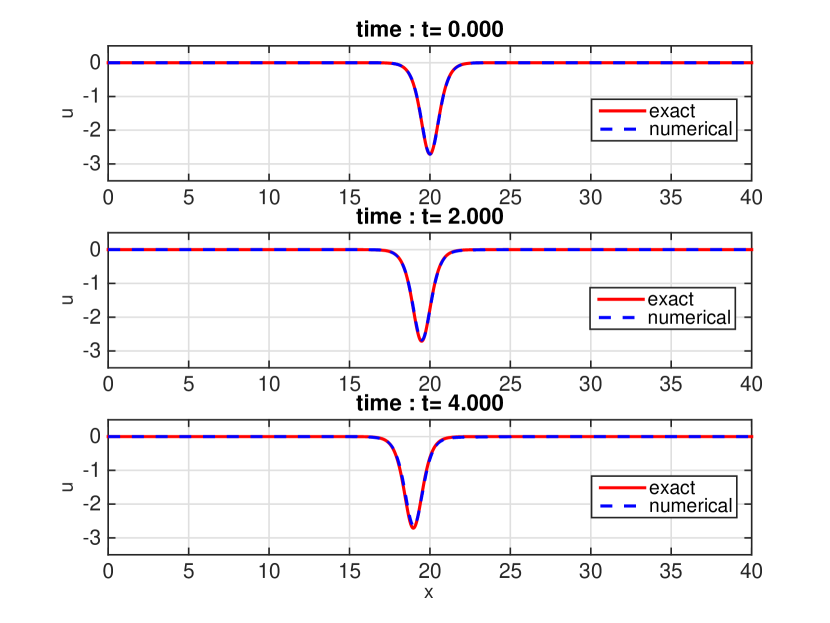
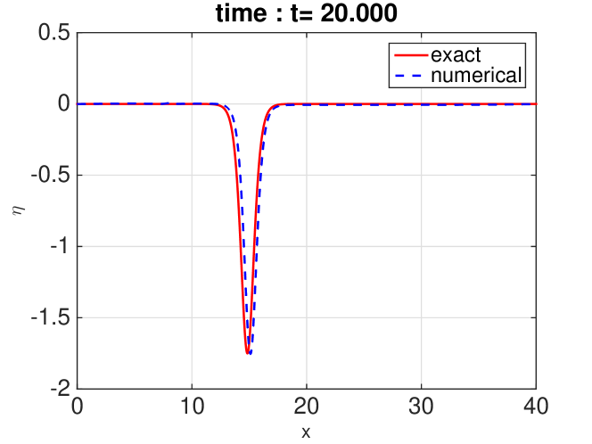
Behavior of the numerical scheme for traveling wave solutions
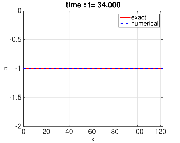
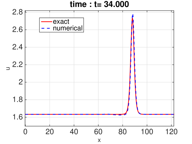
Because of the numerical diffusion, the scheme creates light shifts of the position and of the amplitude of the traveling wave solution in long time. We detail below these aspects for the test case , where the numerical solution is computed with up to the final time . Quantitative results concerning the relative errors in position and amplitude are gathered in Figure 11 (respectively in Table 6).
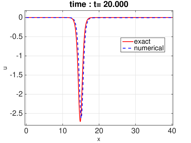
| Position | Amplitude | |||||
|---|---|---|---|---|---|---|
| Numerical | Exact | Relative error | Numerical | Exact | Relative error | |
| 15.105 | 14.840 | 1.7857% | 1.7544 | 1.7500 | 0.2501% | |
| 15.100 | 14.840 | 1.7520% | 2.6227 | 2.7111 | 3.2594% | |
4 Traveling waves collision
Recently, in [7], the authors simulate the collision of two
traveling waves moving in opposite directions in in the BBM-BBM case
(, , , ). Motivated by their results,
we simulated the same phenomenon but for different values of the parameters.
Two behaviors are observable:
-
•
the collision leads to phase shifts and visible dispersive tails which follow each solitary wave,
-
•
the collision suggests a possible blow-up of the -norm in finite time either on the density or on the derivative of .
Our numerical study is restricted to one type of traveling waves collision : the head-on collision when the solitary waves travel in opposite directions and collide. We do not study the overtaking collision (when the solitary waves propagate in the same direction) and we refer the reader for example to [4] for a review of such collisions in the case .
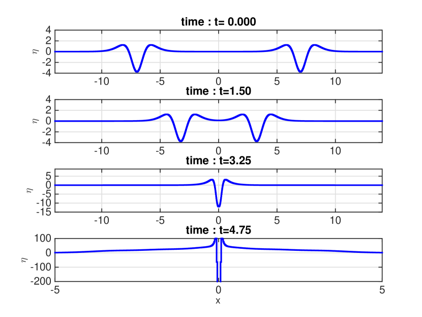
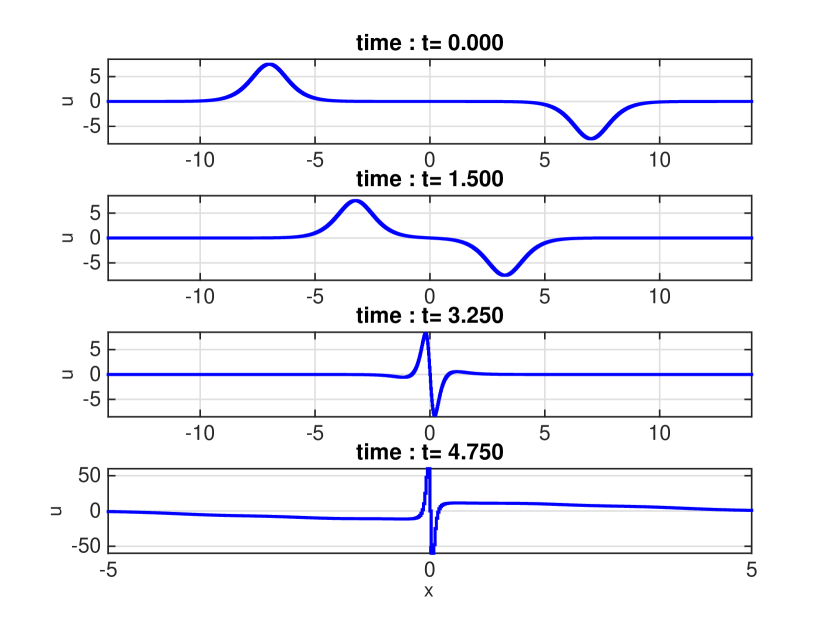
4.1 Finite time blow-up.
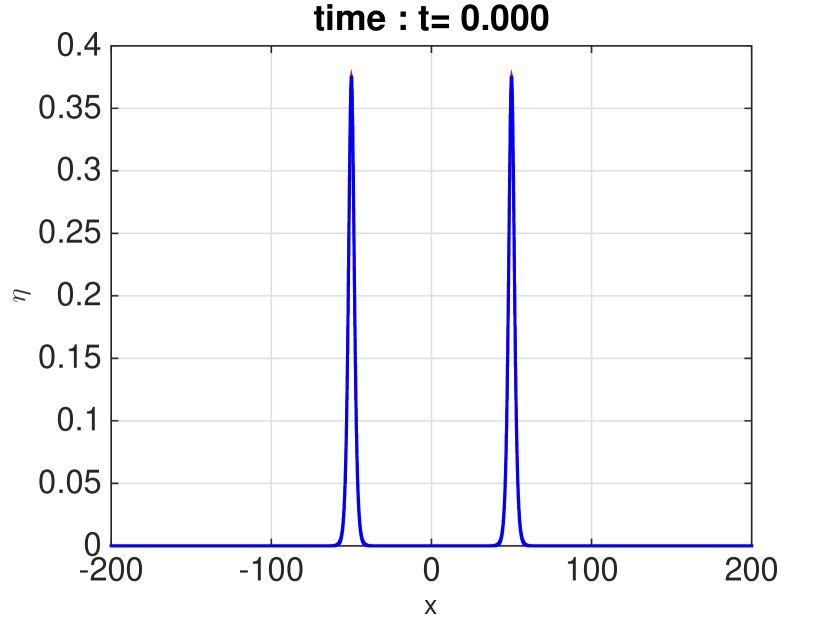
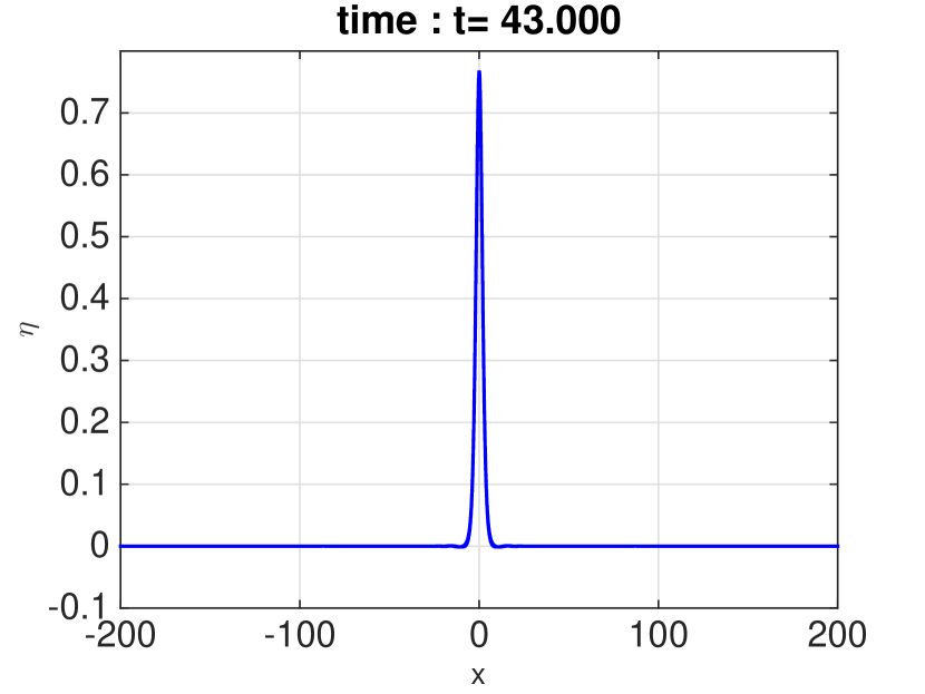
First, we used our numerical results and performed the same experiment described in [7] for (, , , ). The initial condition is fixed to
with
where .
The space domain is fixed at
and initially, the traveling-waves are centered in and
. We choose the same space size and time step as in
[7], namely and . The
simulation suggests that a blow-up occurs while the explosion time appears to be
around as shown in Figure 12, result which is very close to
the one obtained in [7].
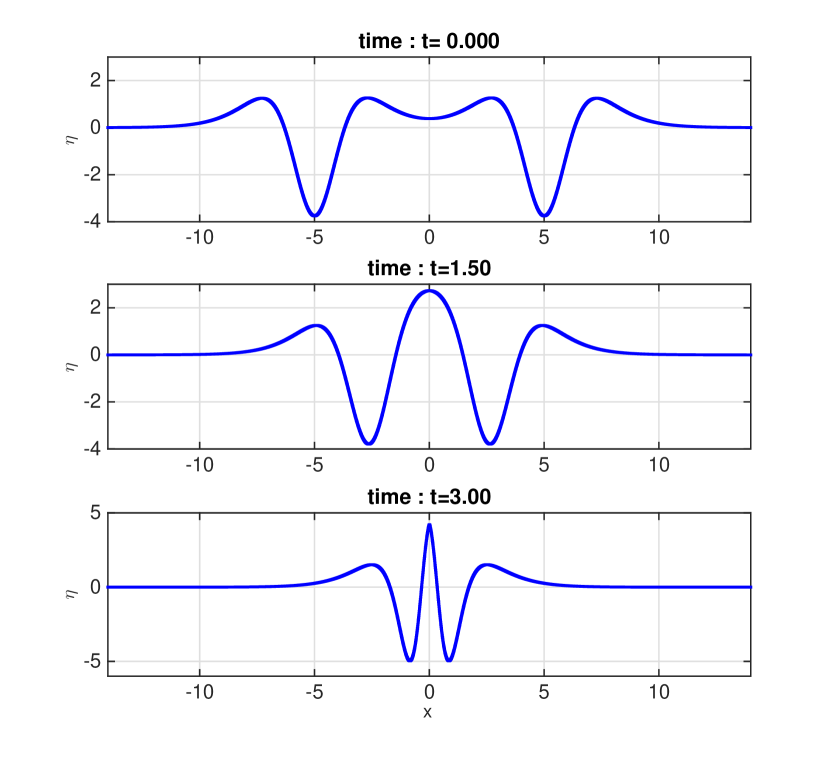
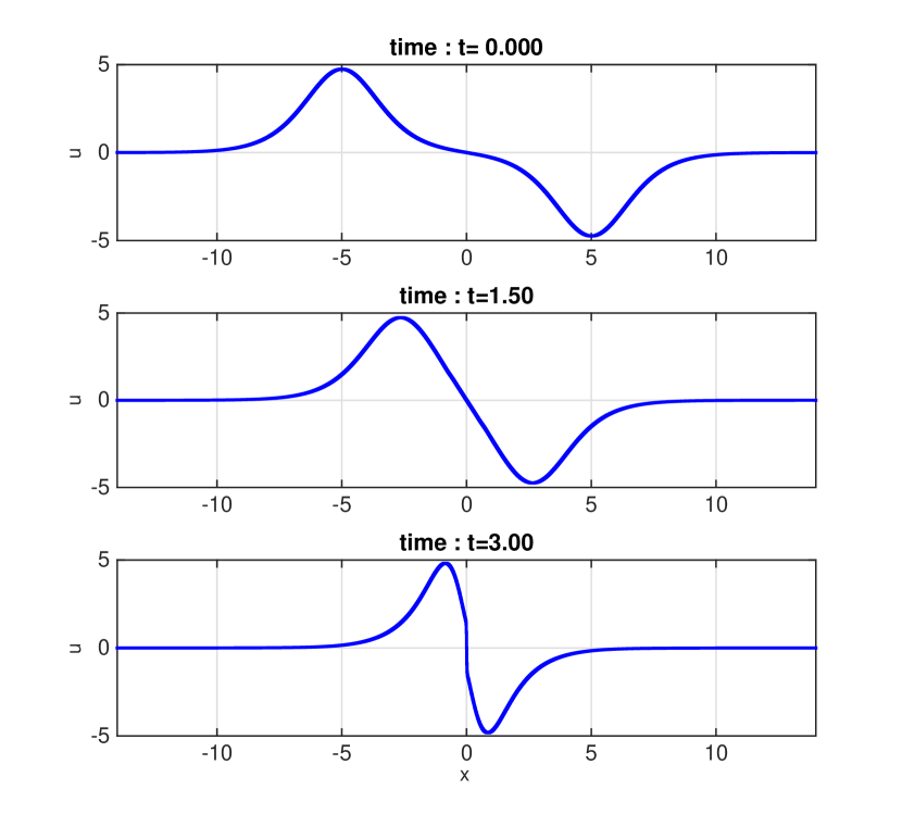
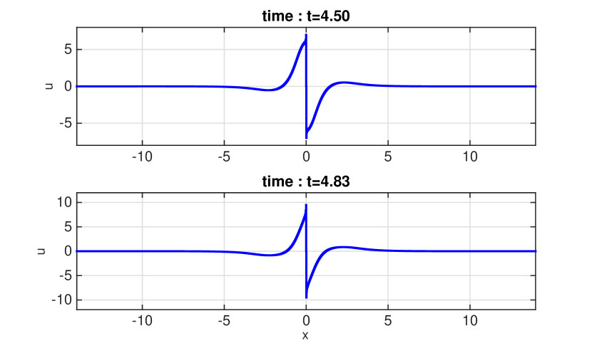
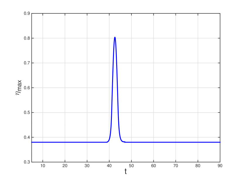
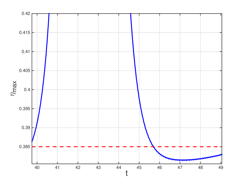
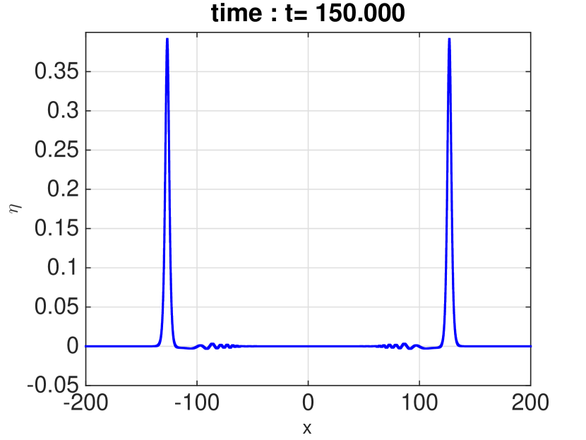
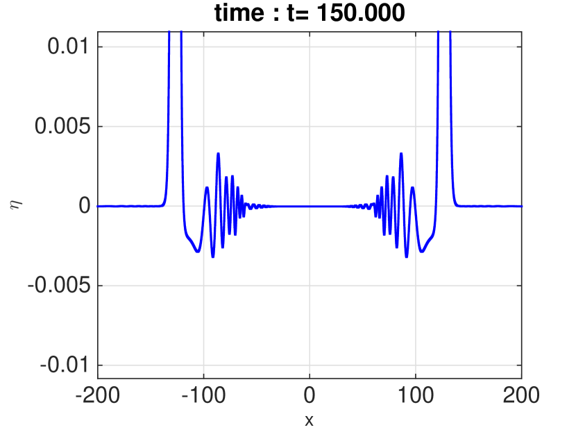
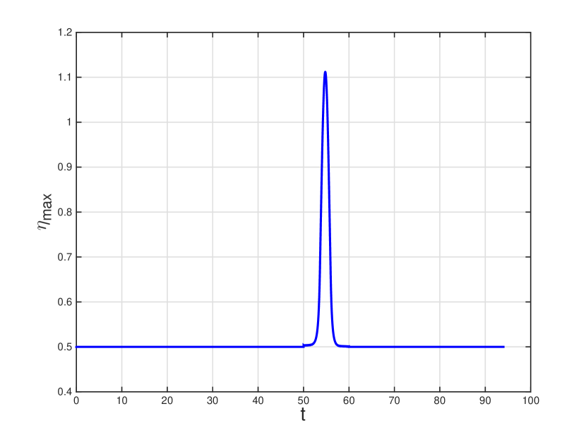
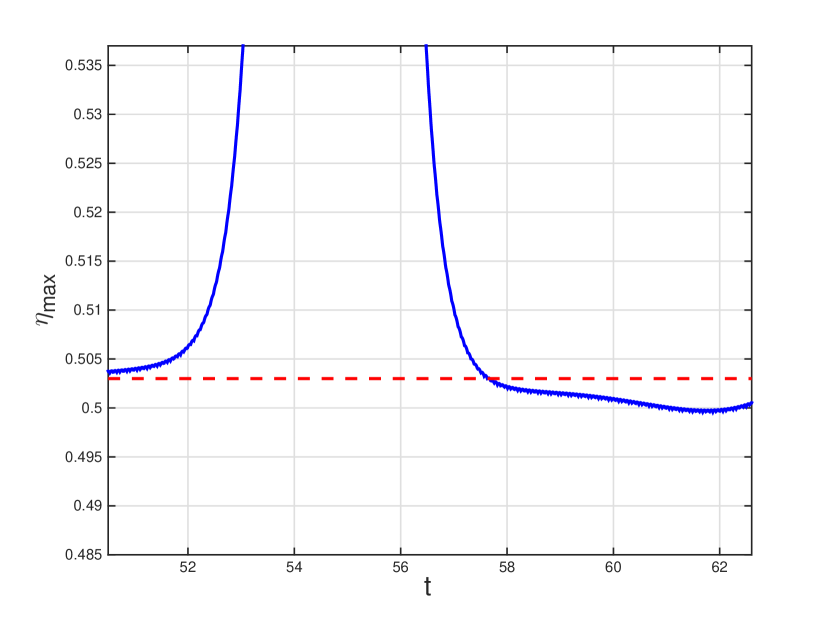
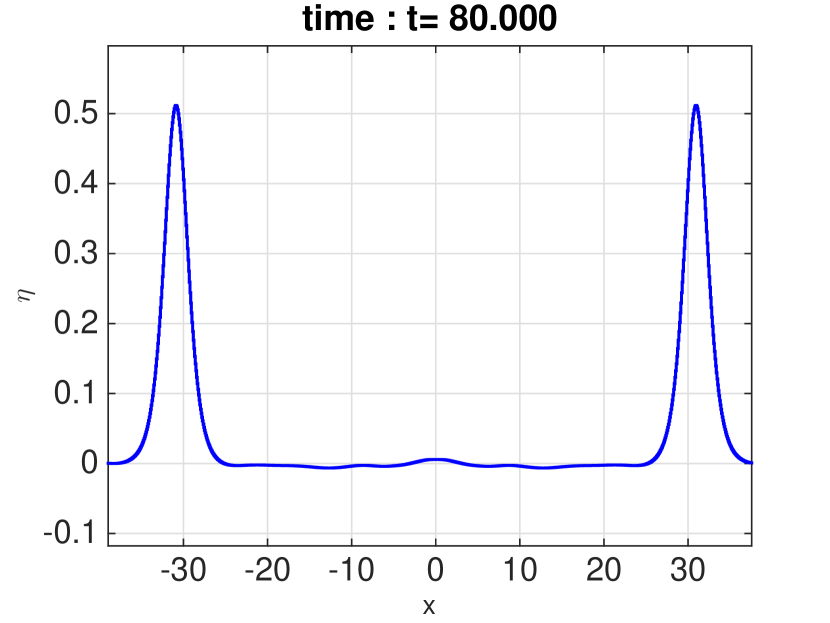
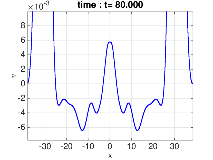
In a second time, we have observed that for the case , solutions of a similar structure as those above are available. The experiment is performed with , and taking the initial value
with
where . The results are gathered in Figure 13. We interpret this figure as a possible blow-up of the -norm on the derivative of .
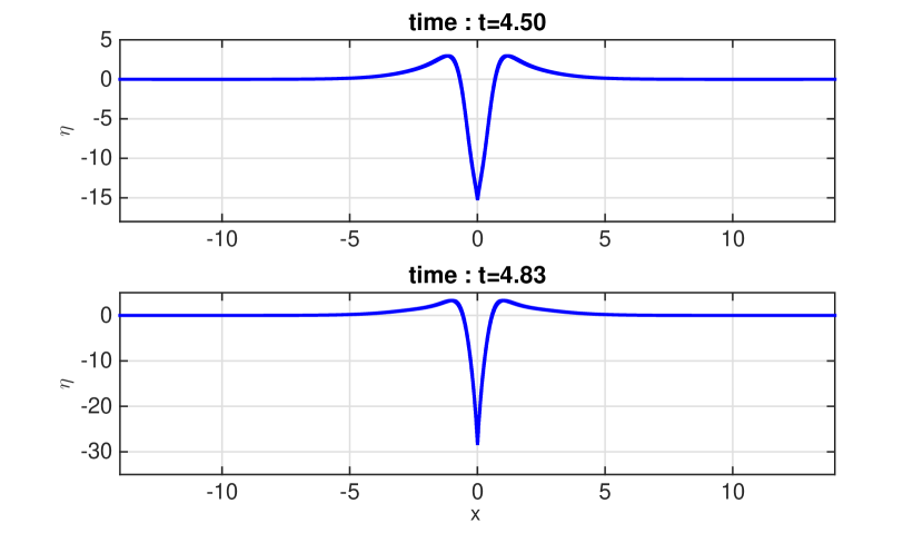
Remark 4.1.
The initial data leading to the ”numerical” blow-up are not physical because the quantity , which is the height of the water column, should be a positive quantity.
4.2 Head-on collision.
In this subsection, we studied two cases where the collision of traveling waves leads to phase shifts and visible dispersive tails which follow each of the waves.
For (), the experiment is performed on the space domain , the space- and time-meshes , and the following initial value
with
where .
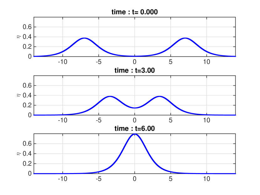
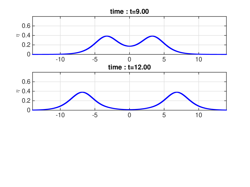
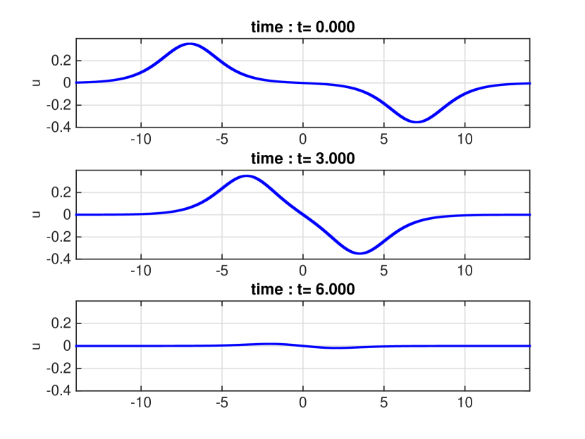
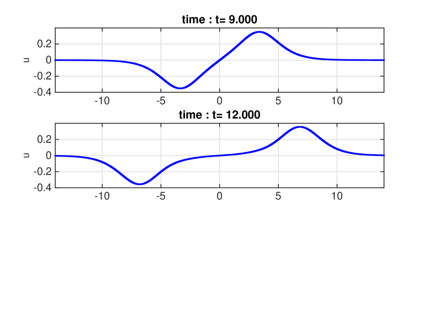
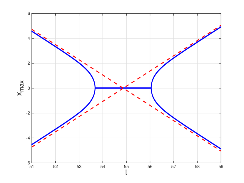
Figure 14 is an overview of the situation, which clearly illustrates that traveling waves emerge from the collision (which occurs at ) without major changes. In reality, some local changes are expected to be produced after the interaction of the waves such as phase-shifts, slight changes in amplitude and dispersive tails. Figures 15-18 illustrate all this expected consequences.
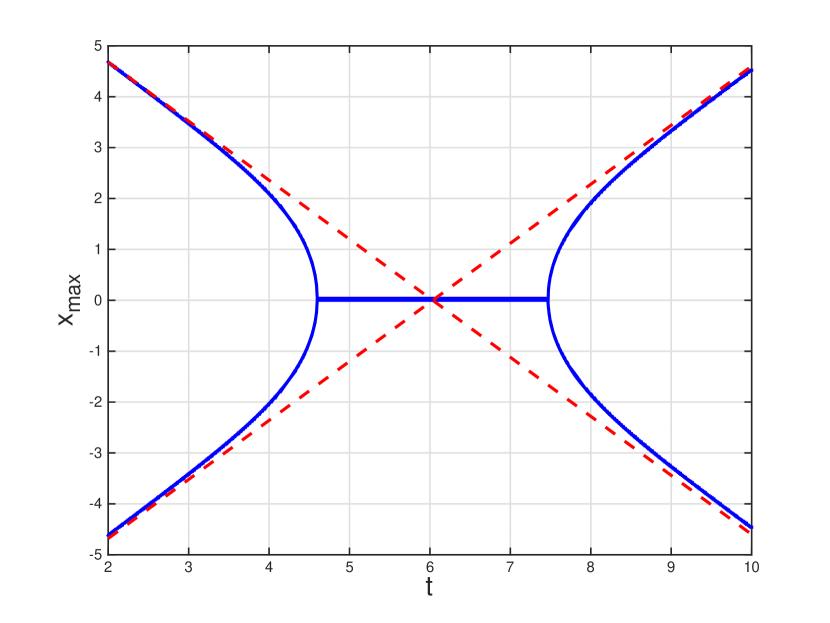
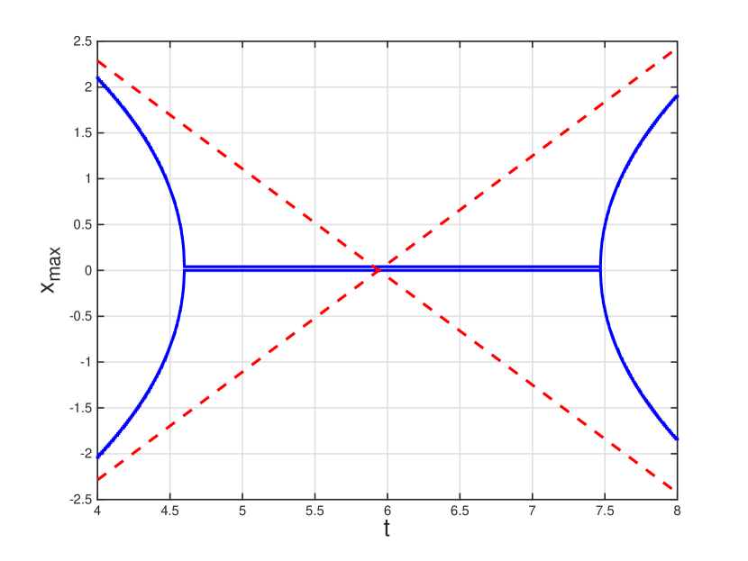
More precisely, Figure 15 illustrates the phase-shift which arises from the collision. The paths of the maximum amplitude of both traveling waves are represented in the -plane, with or without collision. As expected, the traveling waves are delayed by the head-on collision since the phase-shifts are in the opposite direction of their motion. These phase-shifts are characterized by a relative error in velocity equals to for the traveling waves moving from the right to the left and a relative error in velocity equals to for the traveling wave moving from the left to the right.
To visualize the other expected behaviors caused by the head-on collision, we have increased the final time of the numerical simulations. The parameters are now , and the final time . With these new parameters, the collision occurs at . A little modification in the amplitude of the traveling waves is expected from the head-on collision and numerical simulations match this expectation as shown in Figure 16. Indeed, the maximum amplitude of for each traveling wave is lower after the collision than before. For instance, the relative error in maximum amplitude at is . It is worth noting also that the maximum amplitude at the collision () is bigger than the sum of the maximum amplitudes of the two traveling waves before the collision. The maximum elevation during the collision is about bigger than the sum.
Eventually, the collision is inelastic and thus produces some oscillatory dispersive tails, visible in Figure 17 which are magnified in the close up of Figure 18. We point out that this dispersive tail is not due to an instability of the numerical scheme because its amplitude remains constant, regardless of and .
Paths of the traveling waves in the -plane
Magnification around the collision time
Maximum amplitude of against time
Magnification around the collision time
Last but not least, we have performed a numerical experiment to illustrate the head-on collision for . This test case is drawn from [6]. The numerical parameters are fixed to , , and the initial value :
with
where . The traveling waves collide at and emerge with only few changes in phase, amplitude and shape. Figure 19 illustrates for instance the phase-shift by a representation in the -plane of the paths of the maximum amplitude of both waves with (solid line) or without (dashed line) the collision. Once again, a consequence of the collision is a delay of the wave propagation because the phase-shift is oriented in the opposite direction of the motion. The relative error on the velocity of the traveling wave moving from the left to the right is , whereas the relative error on the velocity of the traveling wave moving from the right to the left is equal to .
The changes in maximum amplitude of are summarized in Figure 20. On one hand, both traveling waves have a smaller maximal elevation after the collision (the relative error of maximum amplitude at for instance is equal to ). Secondly, the maximal elevation during the collision is bigger than the sum of both maximum amplitudes ( bigger than the sum).
Maximum amplitude of against time
Magnification around the collision time
Eventually, the dispersive tails resulting from the head-on collision is illustrated in Figure 21 at final time .
Appendix A Consistency error
A.1 Consistency error .
By definition of the consistency error, one has
We define
We define . We will only develop the non linear part and enonce the results for the other parts. By Taylor expansions and Cauchy-Schwarz inequality, one has
In the same way, we develop the -term.
We will develop the non linear part. We denote the following function on
Thus,
Moreover,
We have the same type of equality for . Applying once again the Cauchy-Schwarz inequality gives
Thus, the -term rewrites
Finally, one has
Then, when we sum up all the previous results, we obtain
We recognize the initial equation on the first line. We recall the relation
| (1.113) |
Eventually, when we compute the -norm, we obtain
Thus, one has
with a constant depending of , and their derivatives.
In some cases, is needed. To obtain an upper bound, we perform the same computations and find
A.2 Consistency error .
By definition of the consistency error, on has
We adapt the previous computations with instead of . The only difference is concerning the non linear term
So one has
As for the case, there exists a constant depending on , and their derivatives such that
For , the results are similar to those for .
Acknowledgement
This work was performed within the framework of the LABEX MILYON (ANR-10- LABX0070) of Université de Lyon, within the program ”Investissements d’Avenir” (ANR-11-IDEX-0007) operated by the French National Research Agency (ANR).
References
- [1] C. J. Amick. Regularity and uniqueness of solutions to the Boussinesq system of equations. J. Nonlinear Sci., 54(2):231–247, 1984.
- [2] C. T. Anh. On the Boussinesq/Full dispersion systems and Boussinesq/Boussinesq systems for internal waves. Nonlinear Analysis: Theory, Methods & Applications, 72(1):409–429, 2010.
- [3] D. C. Antonopoulos and V. A. Dougalis. Notes on error estimates for Galerkin approximations of the ’classical’ Boussinesq system and related hyperbolic problems. arxiv, 2010.
- [4] D. C. Antonopoulos and V. A. Dougalis. Numerical solution of the classical Boussinesq system. Mathematics and Computers in Simulation, 82(6):984–1007, 2012.
- [5] D. C. Antonopoulos and V. A. Dougalis. Error estimates for the standard Galerkin-finite element method for the Shallow Water equations. Mathematics of Computation, 85:1143–1182, 2016.
- [6] J. L. Bona and M. Chen. A Boussinesq system for two-way propagation of nonlinear dispersive waves. Physica D: Nonlinear Phenomena, 116(1):191–224, 1998.
- [7] J. L. Bona and M. Chen. Singular Solutions of a Boussinesq System for Water Waves. J. Math. Study, 49(3):205–220, 2016.
- [8] J. L. Bona and R. Smith. A model for the two-way propagation of water waves in a channel. Mathematical Proceedings of the Cambridge Philosophical Society, 79(1):167–182, 1976.
- [9] C. Burtea. Long time existence results for bore-type initial data for BBM-Boussinesq systems. Journal of Differential Equations, 261(9):4825–4860, 2016.
- [10] C. Burtea. New long time existence results for a class of Boussinesq-type systems. Journal de Mathématiques Pures et Appliquées, 106(2):203–236, 2016.
- [11] F. Lagoutière C. Courtès and F. Rousset. Error estimates of finite difference schemes for the Korteweg-de Vries equation. to appear in IMA Journal of Numerical Analysis, arXiv preprint arXiv:1712.02291, https://arxiv.org/abs/1712.02291, 2017.
- [12] F. Chazel. Influence of bottom topography on long water waves. ESAIM: Mathematical Modelling and Numerical Analysis, 41(4):771–799, 2007.
- [13] M. Chen. Exact Traveling-Wave Solutions to Bidirectional Wave Equations. Internat. J. Theoret. Phys., 37(5):1547–1567, 1998.
- [14] M. Chen. Equations for bi-directional waves over an uneven bottom. Mathematics and Computers in Simulation, 62(1):3–9, 2003.
- [15] M. Chen. Numerical investigation of a two-dimensional Boussinesq system. Discrete Contin. Dyn. Syst, 28(4):1169–1190, 2009.
- [16] D. S. Clark. Short proof of a discrete Grönwall inequality. Discrete Applied Mathematics, 16:279–281, 1987.
- [17] V. A. Dougalis D. C. Antonopoulos and D. E. Mitsotakis. Galerkin approximations of periodic solutions of Boussinesq systems. Bulletin of the Greek Mathematical Society, 57:13–30, 2010.
- [18] V. A. Dougalis D. C. Antonopoulos and D. E. Mitsotakis. Numerical solution of Boussinesq systems of the Bona–Smith family. Applied numerical mathematics, 60(4):314–336, 2010.
- [19] P. Daripa and R. K. Dash. A class of model equations for bi-directional propagation of capillary-gravity waves. Internat. J. Engrg. Sci, 41:201–218, 2003.
- [20] D.Pilod F. Linares and J.-C. Saut. Well-Posedness of strongly dispersive two-dimensional surface wave Boussinesq systems. SIAM Journal on Mathematical Analysis, 44(6):4195–4221, 2012.
- [21] C. Wang J.-C. Saut and L. Xu. The Cauchy problem on large time for surface waves type Boussinesq systems II. arXiv preprint arXiv:1511.08824, https://arxiv.org/abs/1511.08824, 2015.
- [22] M. Chen J. L. Bona and J.-C. Saut. Boussinesq equations and other systems for small-amplitude long waves in nonlinear dispersive media. I: Derivation and linear theory. Journal of Nonlinear Science, 12(4):283–318, 2002.
- [23] M. Chen J. L. Bona and J.-C. Saut. Boussinesq equations and other systems for small-amplitude long waves in nonlinear dispersive media: II. The nonlinear theory. Nonlinearity, 17(3):925–952, 2004.
- [24] T. Colin J. L. Bona and D. Lannes. Long Wave Approximations for Water Waves. Archive for Rational Mechanics and Analysis, 178(3):373–410, 2005.
- [25] V. A. Dougalis J. L. Bona and D. E. Mitsotakis. Numerical solution of KdV–KdV systems of Boussinesq equations: I. The numerical scheme and generalized solitary waves. Mathematics and Computers in Simulation, 74(2):214–228, 2007.
- [26] V. A. Dougalis J. L. Bona and D. E. Mitsotakis. Numerical solution of Boussinesq systems of KdV–KdV type: II. Evolution of radiating solitary waves. Nonlinearity, 21(12):2825–2848, 2008.
- [27] D. Lannes. The water waves problem. Mathematical surveys and monographs, 188, 2013.
- [28] J.-C. Saut M. Ming and P. Zhang. Long-time existence of solutions to Boussinesq systems. SIAM Journal on Mathematical Analysis, 44(6):4078–4100, 2012.
- [29] D. H. Peregrine. Calculations of the development of an undular bore. Journal of Fluid Mechanics, 25(2):321–330, 1966.
- [30] J.-C. Saut and L. Xu. The Cauchy problem on large time for surface waves Boussinesq systems. Journal de mathématiques pures et appliquées, 97(6):635–662, 2012.
- [31] M. E. Schonbek. Existence of solutions for the Boussinesq system of equations. Journal of Differential Equations, 42(3):325–352, 1981.
- [32] E. Tadmor. Entropy stability theory for difference approximations of nonlinear conservation laws and related time-dependent problems. Acta Numerica, 12:451–512, 2003.
- [33] D. E. Mitsotakis V. A. Dougalis and J.-C. Saut. On some Boussinesq systems in two space dimensions: Theory and numerical analysis. ESAIM: Mathematical Modeling and Numerical Analysis, 41(5):825–854, 2007.