Symmetries and synchronization in multilayer random networks

Abstract

In the light of the recently proposed scenario of asymmetry-induced synchronization (AISync), in which dynamical uniformity and consensus in a distributed system would demand certain asymmetries in the underlying network, we investigate here the influence of some regularities in the interlayer connection patterns on the synchronization properties of multilayer random networks. More specifically, by considering a Stuart-Landau model of complex oscillators with random frequencies, we report for multilayer networks a dynamical behavior that could be also classified as a manifestation of AISync. We show, namely, that the presence of certain symmetries in the interlayer connection pattern tends to diminish the synchronization capability of the whole network or, in other words, asymmetries in the interlayer connections would enhance synchronization in such structured networks. Our results might help the understanding not only of the AISync mechanism itself, but also its possible role in the determination of the interlayer connection pattern of multilayer and other structured networks with optimal synchronization properties.

I Introduction

Recently, Nishikawa and Motter NishMotter put forward a rather intriguing dynamical phenomenon present in networks of coupled oscillators: the asymmetry-induced symmetry, or asymmetry-induced synchronization (AISync), a scenario where the occurrence of dynamical uniformity and consensus does require certain asymmetries in the underlying network of connections among the oscillators. In many senses, this new phenomenon could be considered as the converse of the well known symmetry breaking process, in which some solutions or the dynamical behavior of a given system do not inherit all the symmetries of the respective governing equationsNishMotter . A general scheme for building networks exhibiting this novel dynamical behavior was just introduced in ZhangNishMotter , where the authors also argue that the asymmetry-induced synchronization should be a rather prevailing behavior in multilayer networks of coupled oscillators. For a recent exposition on AISync, see ZhangMotter Besides its unequivocal interest from a more fundamental point of view, the AISync has also a wide range of possible applications, particularly in synchronization problems pikovsky2001 ; arenas2008 , where the new phenomenon was indeed initially discovered. The AISync challenges frontally the idea that synchronization states should be promoted by symmetric configurations. Nevertheless, there are indeed plenty of relevant examples of synchronization driven by symmetries in networks of oscillator, see, for instance, nicosia2013 ; pecora2014 ; sorrentino2016 ; cho2017 .

Here, we report some new results which may also be classified as a manifestation of AISync. Differently from NishMotter , where the analysis was performed for small scale regular networks, we consider spontaneous synchronization in large scale random networks. More specifically, in the same line of ZhangNishMotter , we consider complex oscillators on multilayer random networksmulti1 ; multi2 and, by exploring some recent ideas and algorithms on optimal synchronizationoptimal , we show that the presence of certain regularities in the interlayer connection pattern tends to diminish the synchronization capability of the coupled oscillators system or, in other words, asymmetries in the connection between layers would enhance synchronization in these kind of structured networks. In this paper, we call structured random network a random multilayer network where inlayer and interlayer connections can have different statistical properties, which could mimic real situations where the layers and the connection among them evolve and are selected differently.

Following the same principles of NishMotter and ZhangNishMotter , we consider both phase and amplitude effects by studying the so-called Stuart-Landau (SL) model with complex oscillators on an $N$-nodes random network

$$\dot{z}_{k}=\left(\alpha^{2}+i\omega_{k}-|z_{k}|^{2}\right)z_{k}+\lambda\sum_{j=1}^{N}a_{kj}(z_{j}-z_{k}),$$ (1)

where $z_{k}$ is the (complex) state of the oscillator located at the $k$ node, with $\omega_{k}$ standing for its natural frequency, which we also assume to be a random variable. The entries $a_{kj}$ correspond here to the usual adjacency matrix for undirected and unweighted networks, and $\lambda$ defines the (real and uniform) coupling strength among the complex oscillators. The real parameter $\alpha$ determines the stability properties of the limit cycle $|z_{k}|^{2}=\alpha^{2}$, which is clearly present for $\lambda=0$. For larger values of $\alpha^{2}$ (compared with $\lambda$), one recovers the paradigmatic Kuramoto model kuramoto1975 ; strogatz2000 ; acebron2005 . For further properties and references on the SL model, see SL1 ; SL2 ; SL3 , for instance. In our simulations, we will use the real version of the Eq. (1). Introducing $z_{k}=\rho_{k}e^{i\theta_{k}}$, we have

$$\dot{\rho}_{k}+i\rho_{k}\dot{\theta}_{k}=\left(\alpha^{2}-i\omega_{k}-\rho_{k}^{2}\right)\rho_{k}+\lambda\sum_{j=1}^{N}a_{kj}\left(\rho_{j}e^{i(\theta_{j}-\theta_{k})}-\rho_{k}\right).$$ (2)

Collecting the real and imaginary parts, one has

$$\dot{\rho}_{k} = \left(\alpha^{2}-\rho_{k}^{2}\right)\rho_{k}-\lambda\sum_{j=1}^{N}{\ell}_{kj}\rho_{j}\cos\left(\theta_{j}-\theta_{k}\right),$$ (3)

$$\rho_{k}\dot{\theta}_{k} = -\omega_{k}\rho_{k}+\lambda\sum_{j=1}^{N}a_{kj}\rho_{j}\sin\left(\theta_{j}-\theta_{k}\right),$$ (4)

where $\ell_{kj}$ stands for the usual network Laplacian matrix components.

It is worth to mention that the self-interacting term in (1) corresponds to the generic behavior near a Hopf bifurcation involving limit cycles, and thus such model is also widely known as Andronov-Hopf oscillators in the literature, see Izhi , for instance. Since we are mainly interested in synchronization properties, a convenient description for the global state of the SL model will be given by the order parameter $r$ defined as

$$r(t)=\left|\frac{1}{N}\sum_{j=1}^{N}e^{i\theta_{j}}\right|.$$ (5)

Clearly, the behavior of the order parameter $r$, which depends only on the oscillator phases, is analogous to the Kuramoto case: $r\approx N^{-1/2}$ for incoherent motion, whereas $r\approx 1$ for a fully synchronized state.

We will consider in this paper the case of multilayer random networks with identical layers, see Fig. 1 for some typical examples.

Figure 1: Typical structured networks considered in this paper. Left: a trilayer random network with identical layers and a diagonal interlayer connection pattern, i.e, connections between the layers are fulfilled only by equivalent nodes in each layers. The diagonal pattern corresponds, probably, to the most regular network topology one might consider in this context. Right: a trilayer random network with the same layers of the previous case, with also the same number of interlayer connections, but with a non-diagonal pattern. The network with diagonal interlayer connections may exhibit some discrete symmetries which are always absent for the non-diagonal case, see Section III for the precise definition and meaning of such symmetries. We have shown that the regular topology (Left) has always impaired synchronization capabilities if compared with the asymmetric case (Right).

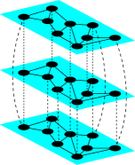
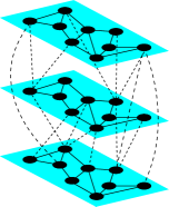
The interlayer connection pattern in these networks can exhibit or not some discrete symmetries corresponding to entire layer permutations. The precise definition and meaning of such symmetries will be discussed in Section III. The most regular connection patterns one may consider in this context are probably those ones with diagonal interlayer connections, see Fig. 1, in the sense that the connection among layers is fulfilled only by equivalent nodes in each layer. We will show that multilayer networks with such regular interlayer connection pattern tend to have impaired synchronization capabilities if compared with similar networks without these regularities in the interlayer connections. Typically, starting with a regular multilayer network, its synchronization properties can be considerably enhanced by applying our optimization rewiring algorithm introduced in optimal for the interlayer connections if one abandons the diagonal pattern. This is, indeed, our main result: the breaking of the interlayer connection symmetries will lead to the enhancement of the network synchronization capabilities, in the same spirit of Motter-Nishikawa AISync NishMotter . We also corroborate one of the main conclusions of ZhangNishMotter , namely that AISync should be a rather generic property of structured networks, i.e., unstructured networks do not exhibit in general such an anti-correlation between symmetries and synchronization.

In the next section, we will revisit the rewiring algorithm introduced in optimal , based on the Gottwald dimensional reduction approach proposed in gottwald2015 , for the optimization of synchronization in the Kuramoto model. Basically, we will show that the same ideas behind the Gottwald dimensional reduction and the optimization algorithm can be conveniently employed also for the SL model. We also derive some new mean-field approximation formulas which have proved to be useful in estimating the efficiency of our algorithm. In Section III, we will consider the synchronization capabilities of large scale multilayer random networks with different interlayer connection patterns, and our main result will be established, with the predictions of the mean-field analysis being confirmed by exhaustive numerical simulations. The last section is devoted to some concluding remarks. We discuss, in particular, the differences between structured and non-structured networks and why the very idea of asymmetry-induced synchronization is much more relevant to the former.

II Dimension reduction for complex oscillators

In optimal , we introduced a rewiring algorithm for the optimization of synchronization in the Kuramoto model by exploring the dimensional reduction approach recently proposed by Gottwald gottwald2015 , which, on the other hand, is based in the introduction of a collective coordinate for the Kuramoto oscillators in the same spirit of the Ott-Antonsen ansatz ott2008 ; ott2009 . The extension of this optimization scheme for the SL model will be instrumental in the present analysis. The Gottwald collective ansatz gottwald2015 can be adapted for the present case as

$$z_{k}(t)=\rho_{k}(t)e^{i\left(\omega_{k}\beta(t)+\Omega t+\varphi_{0}\right)},$$ (6)

which will be able to capture all the essential properties of the synchronized states for the SL model. The offset parameter $\varphi_{0}$ can be conveniently set to zero without loss of generality, since the SL model is an autonomous system and $\varphi_{0}$ can be easily absorbed by a simple shift in $t$. From the equations of motion (3) and (4), one has the following dynamical equations for the real variables $\rho_{k}$ and $\beta$

$$\dot{\rho}_{k}=F_{k}(\rho_{j},\beta)=\left(\alpha^{2}-\rho_{k}^{2}\right)\rho_{k}-\lambda\sum_{j=1}^{N}\ell_{kj}\rho_{j}\cos\beta(\omega_{j}-\omega_{k}),$$ (7)

and

$$\rho_{k}\omega_{k}\dot{\beta}=(\omega_{k}-\Omega)\rho_{k}+\lambda\sum_{j=1}^{N}a_{kj}\rho_{j}\sin\beta(\omega_{j}-\omega_{k}).$$ (8)

Ir order to cast Eq. (8) in a more convenient form, we multiply both sides by $\rho_{k}\omega_{k}$

$$\rho_{k}^{2}\omega_{k}^{2}\dot{\beta}=\rho_{k}^{2}\omega_{k}^{2}-\Omega\rho_{k}^{2}\omega_{k}+\lambda\sum_{j=1}^{N}a_{kj}\omega_{k}\rho_{k}\rho_{j}\sin\beta(\omega_{j}-\omega_{k}).$$ (9)

Now, summing over $1\leq k\leq N$, dividing by $N$ and rearranging the terms, one gets

$$\dot{\beta}=G(\rho_{j},\beta) = 1-\Omega\frac{\left\langle\rho_{k}^{2}\omega_{k}\right\rangle}{\left\langle\rho_{k}^{2}\omega_{k}^{2}\right\rangle}$$

$$+\frac{\lambda}{N\left\langle\rho_{k}^{2}\omega_{k}^{2}\right\rangle}\sum_{k=1}^{N}\sum_{j=1}^{N}a_{kj}\omega_{k}\rho_{k}\rho_{j}\sin\beta(\omega_{j}-\omega_{k}),$$

where the brackets denote simple averages as, for instance, in

$$\left\langle\rho_{k}^{2}\omega_{k}^{2}\right\rangle=\frac{1}{N}\sum_{k=1}^{N}\rho_{k}^{2}\omega_{k}^{2}.$$ (11)

In contrast with the case of the Kuramoto model considered in optimal , one cannot assure, in principle, that the rigid rotation $\Omega$ vanishes for a synchronized state in networks with a frequency distribution $g(\omega)$ with null average, for instance. In fact, for a fixed point $\left(\bar{\rho}_{j},\bar{\beta}\right)$ of (7) and (II), we will have

$$\Omega=\frac{\left\langle\bar{\rho}^{2}_{k}\omega_{k}\right\rangle}{\left\langle\bar{\rho}_{k}^{2}\right\rangle}.$$ (12)

Notice that for uniform $\bar{\rho}_{k}$ (the Kuramoto limit), $\Omega$ does indeed vanish if $\langle\omega_{k}\rangle=0$ and, moreover, in this case equation (II) will coincide with the Gottwald dimensionally reduced equation introduced in gottwald2015 for the Kuramoto model. Hereafter, unless explicitly stated otherwise, we will assume we are dealing with symmetric distributions $g(\omega)$ with null average.

From our ansatz (6), it is clear that the fixed points $\left(\bar{\rho}_{j},\bar{\beta}\right)$ of (7) and (II) correspond to synchronized states. Furthermore, for small values of $\bar{\beta}$, they will typically be optimally synchronized states, in the sense that they will exhibit an order parameter $r$ given by (5) close to 1. For large scale networks, one can estimate $r$ for a given fixed point, with good accuracy, by using a mean-field approach. Directly from (5) and (6), we have

$$r(\beta)=\left\langle\cos\beta\omega_{k}\right\rangle=\int d\omega\,g(\omega)\cos\beta\omega$$ (13)

for a symmetric distributions $g(\omega)$ of frequencies with null average. The most commonly used distributions in the literature are the normal and the homogeneous, which will correspond, respectively, to the following mean-field expressions for $r$

$$r_{\rm n}=\exp\left(-\frac{1}{2}\beta^{2}\sigma_{\omega}^{2}\right)$$ (14)

and

$$r_{\rm u}=\frac{\sin\sqrt{3}\beta\sigma_{\omega}}{\sqrt{3}\beta\sigma_{\omega}}.$$ (15)

For both case, we have

$$r\approx 1-\frac{1}{2}\beta^{2}\sigma_{\omega}^{2}$$ (16)

for small $\beta$. Notice that synchronized states with $r\approx 1$ require also a small frequency standard deviation $\sigma_{\omega}=\sqrt{\left\langle\omega^{2}_{k}\right\rangle}$.

We are quite sure about the existence of the fixed points $\left(\bar{\rho}_{j},\bar{\beta}\right)$ of (7) and (II) for coupling constants $\lambda$ larger than some threshold value $\lambda_{c}$. In fact, we will show that we can even estimate $\lambda_{c}$ with good accuracy from the Gottwald dimensionally reduced approach. The fixed points $\left(\bar{\rho}_{j},\bar{\beta}\right)$ correspond, of course, to the zeros $F_{k}(\bar{\rho}_{j},\bar{\beta})=0$ and $G(\bar{\rho}_{j},\bar{\beta})=0$. Since we are dealing with a system of non-linear equations, we can have effectively several fixed points, some of them might be even dynamically stable. However, for our purposes, we will focus on the fixed point near $\rho_{k}=\alpha$ and $\beta=0$, which turns out to be always dynamically stable. Let us consider a linear approximation for the system (7) and (II) around this point. By introducing $\rho_{k}=\alpha+\delta_{k}$, we have

$$\dot{\delta}_{k} = -2\alpha^{2}\delta_{k}-\lambda\sum_{j=1}^{N}\ell_{kj}\delta_{j},$$ (17)

$$\dot{\beta} = 1-\lambda{\cal L}\beta-\frac{2\Omega\left\langle\omega_{k}\delta_{k}\right\rangle}{\alpha\left\langle\omega^{2}_{k}\right\rangle},$$ (18)

with

$${\cal L}=\frac{\boldsymbol{\omega}^{T}L\boldsymbol{\omega}}{\boldsymbol{\omega}^{T}\boldsymbol{\omega}},$$ (19)

where $L=[\ell_{kj}]$ is the usual Laplacian matrix for the network and $\boldsymbol{\omega}$ is the $N$-dimensional vector formed by the oscillator natural frequencies, $\boldsymbol{\omega}=[\omega_{k}]$. Since the Laplacian matrix is a non-negative diagonalizable matrix, $\lambda L+2\alpha^{2}\boldsymbol{I}$ is invertible for $\alpha\neq 0$ and $\lambda>0$, and hence the linearized fixed points are $\bar{\rho}_{k}\approx\alpha$ and

$$\bar{\beta}\approx\frac{1}{\lambda\cal L},$$ (20)

which, as we will see below, are indeed good approximations for $\left(\bar{\rho}_{j},\bar{\beta}\right)$ for large values of $\lambda\cal L$. It is convenient for our purposes here to go one step further by expanding the equations (7) up to second order, leading to the following second order approximation in $\beta$ for the fixed point $\bar{\rho}_{k}$

$$\bar{\rho}_{k}\approx\alpha-\frac{\lambda\bar{\beta}^{2}}{2\alpha}\sum_{i=1}^{N}\sum_{j=1}^{N}m_{ki}a_{ij}(\omega_{j}-\omega_{i})^{2},$$ (21)

where

$$[m_{ki}]=\left(\frac{\lambda}{\alpha^{2}}L+2\boldsymbol{I}\right)^{-1}.$$ (22)

Also, from (21), we have the following approximation for the synchronized state rigid rotation $\Omega$ given by (12)

$$\Omega\approx\langle\omega_{k}\rangle-\frac{\lambda\bar{\beta}^{2}}{N\alpha^{2}}\sum_{k=1}^{N}\sum_{i=1}^{N}\sum_{j=1}^{N}m_{kj}a_{ij}\omega_{i}(\omega_{j}-\omega_{i})^{2}.$$ (23)

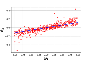
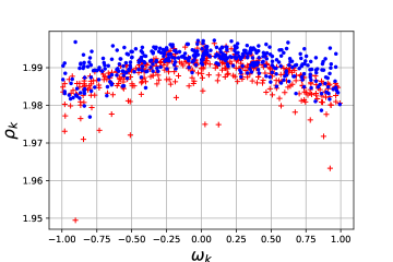
Notice that for large $\alpha$ we get from (21), as expected, the Kuramoto limit of uniform amplitudes, $\bar{\rho}_{k}=\alpha$, for which $\Omega$ vanishes for $\langle\omega_{k}\rangle=0$. We have performed exhaustive numerical simulations and could verify the approximations (20) and (21) with good accuracy, see Fig. 2 for some typical results.

Figure 2: Typical asymptotic behavior of a synchronized state in the SL system (1), where $z_{k}=\rho_{k}e^{i\theta_{k}}$. The depicted cases correspond to an Erdös-Rényi random network with 400 nodes, with average degree $\langle d_{k}\rangle=8.26$, $\alpha=2$, $\lambda=1$, and $\omega_{k}$ draw from the interval $(-1,1)$ with uniform distribution. Top: the 400 points $(\omega_{k},\theta_{k}(t))$ for $t$ large enough to reach a stationary regime (namely in this case, $t=5$), starting from random initial conditions. The straight line has inclination given by the prediction (20), $\bar{\beta}=0.12$, showing that the ansatz (6), which implies $\theta_{k}=\bar{\beta}\omega_{k}+\Omega t$ in the stationary regime, is indeed a good approximation. The rigid rotation in this case is $\Omega=0.02$. Bottom: the red crosses are the points $(\omega_{k},\rho_{k}(t))$ in the stationary regime, while the blue circles correspond to the prediction (21), confirming a good overall accuracy for our ansatz (6).

Also, it is worth noting that $\rho_{k}=0$, which of course corresponds to $z_{k}=0$ in the original SL equations (1), irrespective of the value of $\beta$, correspond to fixed points in our system. Such (continuous) family of fixed points are rather spurious for our purposes since they not correspond effectively to synchronized states. However, since

$$\frac{\partial F_{k}}{\partial\rho_{j}}=\alpha^{2}\delta_{kj}-\lambda\ell_{kj}\cos\beta(\omega_{j}-\omega_{k})$$ (24)

at $\rho_{k}=0$, we see that such points can in principle be attractive for sufficiently large values of $\lambda$ and certain ranges of $\beta$. This is a point to keep in mind, excessively large values of $\lambda$ can push the system into this attraction basin, jeopardizing the possibility of attaining eventually a synchronized state using the ansatz (6).

Let us now focus on the estimation of the synchronization threshold $\lambda_{c}$ from the mean-field approach. For sake of simplicity, let us consider the Kuramoto limit $\rho_{k}=\alpha$. Notice that one can express

$${\cal D}(\beta)=\frac{1}{N\sigma_{\omega}^{2}}\sum_{k=1}^{N}\sum_{j=1}^{N}a_{kj}\omega_{k}\sin\beta(\omega_{j}-\omega_{k})$$ (25)

in the mean-field approximation as

$${\cal D}(\beta) = \frac{\left\langle d_{k}\right\rangle}{\sigma_{\omega}^{2}}\int d\omega g(\omega)\omega\int d\omega^{\prime}g(\omega^{\prime})\sin\beta(\omega^{\prime}-\omega)$$ (26)

$$= \frac{\left\langle d_{k}\right\rangle}{2\sigma_{\omega}^{2}}\frac{d}{d\beta}r^{2}(\beta),$$

where $\langle d_{k}\rangle$ stands for the average degree of the network and $r(\beta)$, the mean-field approximation for the order parameter (5), is given by Eq. (13). Since equation (II) in the Kuramoto limit corresponds to

$$\dot{\beta}=1+\lambda{\cal D}(\beta),$$ (27)

the value of $\lambda_{c}$ necessary to assure the existence of a zero for the right-handed side of (27) can be inferred from the minimum of ${\cal D}(\beta)$. One can easily determine the function $\cal D$ for normal and uniform distributions, for instance. From the expressions (14), (15), and (26), one has

$${\cal D}_{\rm n}=-\left\langle d_{k}\right\rangle\beta e^{-\beta^{2}\sigma_{\omega}^{2}}$$ (28)

and

$${\cal D}_{\rm u}=-\frac{\left\langle d_{k}\right\rangle}{\beta\sigma_{\omega}^{2}}\left(\frac{\sin^{2}\sqrt{3}\beta\sigma_{\omega}}{3\beta^{2}\sigma_{\omega}^{2}}-\frac{\sin 2\sqrt{3}\beta\sigma_{\omega}}{2\sqrt{3}\beta\sigma_{\omega}}\right),$$ (29)

which respective aspects are depicted in Fig. 3 for some typical large random networks.

Figure 3: The aspect for the function ${\cal D}(\beta)$ given by (26) for a normal (top) and uniform (bottom) frequency distributions $g(\omega)$ with null average. Top: A Barabasi-Albert network with 1000 nodes, average degree $\langle d_{k}\rangle=5.98$, and a normal frequency distribution with $\sigma_{\omega}=3/2$. Bottom: An Erdös-Rényi network with 1000 nodes, average degree $\langle d_{k}\rangle=7.39$, and a uniform frequency distribution in the interval $(-2,2)$. For both cases, the lines are the mean-field predictions, Eq. (28) and Eq. (29), and the blue circles correspond to the respective numerical values calculated from (25). Notice that ${\cal D}^{\prime}(0)$ is given by $-\cal L$, defined by (19).

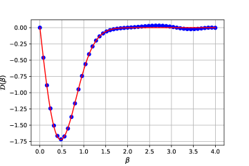
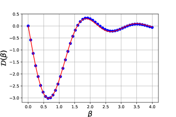
For both cases, we have a simple expression for the synchronization threshold,

$$\lambda_{c}=\gamma\frac{\sigma_{\omega}}{\langle d_{k}\rangle}.$$ (30)

where $\gamma=\sqrt{2e}$ for the normal distribution case. For uniform distributions, one can evaluate $\gamma$ by noticing that the global minimum of

$$f(x)=\frac{d}{dx}\left(\frac{\sin x}{x}\right)^{2}.$$ (31)

can be easily determined numerically, and we will have finally $\gamma\approx 2.14$. Notice that $\sqrt{2e}\approx 2.33$ and, hence, the synchronization thresholds are rather close for both distributions. The key point, however, is the dependence of $\lambda_{c}$ on $\sigma_{\omega}$ and ${\langle d_{k}\rangle}$.

II.1 The optimization algorithm

We are now ready to define precisely what we understand by the network synchronization capability and how to formulate an optimization scheme in order to enhance it. Of course, we want to facilitate the appearance of fully synchronized regimes for the network, and this can be achieved, for instance, demanding a smaller threshold value of $\lambda_{c}$, which clearly would correspond to a network where a synchronization could occur more easily. Furthermore, we could also demand a better stability of the fixed points $\left(\bar{\rho}_{j},\bar{\beta}\right)$, which, on the other hand, would correspond to a more robust synchronized state. The stability of the fixed point is determined by the eigenvalues of the Jacobian matrix $J=\frac{\partial(F_{k},G)}{\partial(\rho_{j},\beta)}$. We are mainly concerned with the fixed point near $\rho_{k}=\alpha$ and $\beta=0$ and, hence, we will approximate the Jacobian matrix at the fixed point $\left(\bar{\rho}_{j},\bar{\beta}\right)$ by the Jacobian matrix at $\left(\alpha,0\right)$,

$$J=\left[\begin{array}[]{c|c}-(\lambda L+2\alpha^{2}\boldsymbol{I})&0\\ \hline\cr-\frac{2\Omega}{\alpha\langle\omega^{2}\rangle}\boldsymbol{\omega}^{T}&-\lambda{\cal L}\end{array}\right].$$ (32)

Since (32) is a block matrix, its eigenvalues can be easily determined. Notice that any block matrix of the type (32) can be decomposed as

$$\left[\begin{array}[]{c|c}A&0\\ \hline\cr B&C\end{array}\right]=\left[\begin{array}[]{c|c}A&0\\ \hline\cr B&\boldsymbol{I}\end{array}\right]\left[\begin{array}[]{c|c}\boldsymbol{I}&0\\ \hline\cr 0&C\end{array}\right],$$ (33)

where the consistent orders of the sub-hmatrices are implicitly assumed. The eigenvalues $\varpi$ of the Jacobian matrix $J$ corresponds to the roots of the characteristic polynomial $\det\left(J-\varpi\boldsymbol{I}\right)=0,$ which can be decomposed according to (33) as

$$\det\left(J-\varpi\boldsymbol{I}\right)=\left(\lambda{\cal L}+\varpi\right)\det\left((\lambda L+2\alpha^{2}\boldsymbol{I})+\varpi\boldsymbol{I}\right)=0.$$ (34)

It is clear that the eigenvalues of the Jacobian matrix $J$ are $-\lambda{\cal L}$ and those ones of the $N\times N$ matrix $-(\lambda L+2\alpha^{2}\boldsymbol{I})$. Moreover, since all of them are negative, the fixed point will indeed be always dynamically stable, irrespective of the value of the rigid rotation $\Omega$. By demanding a larger value of $\cal L$ given by (19), one simultaneously achieves both optimization conditions: a smaller effective threshold value $\lambda_{c}$ and a more robust synchronized state. The maximization of ${\cal L}$ is exactly the optimization goal of the algorithm introduced in optimal , which we have just established to be also valid in the present case of the SL model.

Now, we can envisage a simple hill-climb rewiring optimization algorithm consisting, roughly, in eliminating a random edge of the network and substituting it with a new randomly chosen one. If the resulting network is still connected and has a larger value of $\cal L$, the modification is accepted and the procedure is repeated. This algorithm typically produces networks with far better synchronization capabilities, and its usage requires quite modest computational resources, even for large networks, since (19) is a simple quadratic function. For our purposes here, we will use $\cal L$ as a quantifier for the network synchronization capability, the larger value of $\cal L$, the better synchronization properties of the network. This conclusion is totally compatible with the numerical works done before for the Kuramoto model louzada2012 ; li2013 ; zhang2013 and also for the so-called Kuramoto model with inertia pinto2014 , which is particularly relevant to the study of power linesfilatrella2008 ; motter2013 . We have confirmed here, by exhaustive numerical simulations, the validity of this conclusion also for the SL case.

We can improve considerably the performance of our algorithm by exploring some heuristics. For instance, any Laplacian matrix can be decomposed as the sum of elementary matrices for the edges

$$L=\sum_{e(i,j)}L_{(i,j)},$$ (35)

where the sum is to be performed over all the edges $e(i,j)$ in the network, and $L_{(i,j)}$ is the elementary Laplacian matrix corresponding to the sole edge connecting the nodes $i$ and $j$. From the decomposition (35), we have that (19) can be written as

$${\cal L}=\sum_{e(i,j)}\frac{\boldsymbol{\omega}^{T}L_{(i,j)}\boldsymbol{\omega}}{\boldsymbol{\omega}^{T}\boldsymbol{\omega}} = \sum_{e(i,j)}\frac{(\omega_{i}-\omega_{j})^{2}}{\boldsymbol{\omega}^{T}\boldsymbol{\omega}}$$

$$= \sum_{k=1}^{N}\frac{d_{k}\omega_{k}^{2}}{\boldsymbol{\omega}^{T}\boldsymbol{\omega}}-2\sum_{e(i,j)}\frac{\omega_{i}\omega_{j}}{\boldsymbol{\omega}^{T}\boldsymbol{\omega}},$$

from where one can immediately recognize if a certain rewiring step in our algorithm will be successful or not. Besides of keeping the connectedness of the network, the value of $|\omega_{i}-\omega_{j}|$ for the new link must be larger than the original one. For a random network with random frequencies, one can also estimate ${\cal L}$ from a mean field approximation. For symmetric frequencies distribution $g(\omega)$ with null average, the last term in (II.1) vanishes, leading to ${\cal L}\approx\langle d_{k}\rangle$, which we have indeed corroborated in our numerical simulations. Also from a mean field approximation, we can estimate ${\cal L}_{\rm max}$, the largest possible value for ${\cal L}$ obtained by applying our algorithm to a random network. It will correspond to the connected network where the weakest edges (smallest values of $|\omega_{i}-\omega_{j}|$) where substituted with the strongest ones (largest values of $|\omega_{i}-\omega_{j}|$). In this case, the last term in (II.1) does not vanish anymore since the edges are no more randomly scattered in the adjacency matrix, see Fig. 4.

Figure 4: Top: nonzero entries of the adjacency matrix for a random Erdös-Rényi network with 50 nodes and 153 edges ($\langle d_{k}\rangle=6.12$). The nodes are sorted and numbered according to the corresponding values of $\omega_{k}$, which is assumed to be a random variable. The edges are randomly scattered in the matrix, implying the vanishing of the last term in the Eq. (II.1). Bottom: the corresponding optimal rewiring for the same network. The edges are now concentrated in the corners of the matrix, and we can estimate (II.1) by restricting the sum to the area occupied by the edges in the matrix.

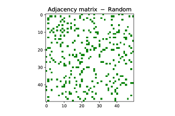
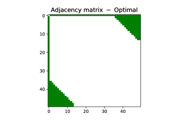
Let us suppose we have a random network with average degree $\langle d_{k}\rangle$, where its $N$ nodes have been sorted and numbered accordingly to the respective values of the random variable $\omega_{k}$. The number of edges will be $N_{\rm e}=N\langle d_{k}\rangle/2$ and we can estimate ${\cal L}_{\rm max}$ for a normal distribution of frequencies $g(\omega)$ as (see Fig. 4)

$${\cal L}_{\rm max}^{\rm(n)}\approx\frac{2N}{\sigma^{2}_{\omega}}\int_{-\infty}^{\infty}du\,g(u)\int_{\frac{\omega_{*}}{\sqrt{2}}}^{\infty}dv\,g(v)v^{2},$$ (37)

where $\omega_{*}$ is such that

$$\int_{-\infty}^{\infty}du\,g(u)\int_{\frac{\omega_{*}}{\sqrt{2}}}^{\infty}dv\,g(v)=\frac{\langle d_{k}\rangle}{2(N-1)},$$ (38)

which leads to

$$\frac{1}{N}{\cal L}_{\rm max}^{\rm(n)}\approx\frac{\langle d_{k}\rangle}{N-1}+\frac{2\kappa e^{-\kappa^{2}}}{\sqrt{\pi}},$$ (39)

with

$${\rm erfc}(\kappa)=\frac{\langle d_{k}\rangle}{N-1}.$$ (40)

In an analogous way, one can obtain for the case of a uniform frequency distribution $g(\omega)$

$$\frac{1}{N}{\cal L}_{\rm max}^{\rm(u)}=\frac{\langle d_{k}\rangle}{N-1}\left(3\frac{\langle d_{k}\rangle}{N-1}-8\sqrt{\frac{\langle d_{k}\rangle}{N-1}}+6\right).$$ (41)

By construction, our algorithm preserves the total number of edges and, consequently, also the average degree $\langle d_{k}\rangle$. For a network with $N$ notes, the maximum possible value for $\langle d_{k}\rangle$ is $N-1$, which corresponds to the all-to-all connection topology. In this case, there is no room for optimization and ${\cal L}_{\rm max}\approx\langle d_{k}\rangle$ for large $N$. Fig. 5 depicts the maximum gain in the network synchronization capability,

Figure 5: The maximum gain (42) in the network synchronization capability achieved by using the optimization algorithm. The (blue) dashed and the (red) solid lines correspond, respectively, to the normal and uniform distribution cases. The algorithm is typically much more efficient for sparse networks. For instance, for the networks of Fig. 3, one has $\frac{\langle d_{k}\rangle}{N-1}\approx 0.006\sim 0.008$, and ${\cal L}$ could be enlarged by a factor of 5 and 8, respectively, by using the algorithm for the uniform and normal distribution cases

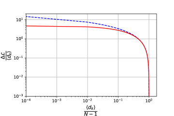
defined as

$$\Delta{\cal L}={\cal L}_{\rm max}-\langle d_{k}\rangle,$$ (42)

obtained by employing our algorithm on a large random network with average degree $\langle d_{k}\rangle$. The algorithm is typically much more efficient for sparse networks, i.e., for networks with $\frac{\langle d_{k}\rangle}{N-1}\ll 1$.

III Interlayer symmetries and synchronization

Let us now consider the synchronization capability of multilayer networks as those ones depicted in Fig. 1 in the light of the results of last Section. We are mainly interested here in multilayer networks built from identical layers, which are supposed to have $N$ nodes each and Laplacian matrix $L^{(0)}$. The Laplacian matrix of a generic $k$-layer networks built from such identical layers will be given by the following $kN\times kN$ symmetric matrix

$$L=\left[\begin{array}[]{c|c|c|c}\displaystyle L^{(0)}+D_{1}&-{C}_{12}&\cdots&-C_{1k}\\ \hline\cr-C_{21}&L^{(0)}+D_{2}&\cdots&-C_{2k}\\ \hline\cr\vdots&\vdots&\ddots&\vdots\\ \hline\cr-{C}_{k1}&\cdots&\cdots&L^{(0)}+D_{k}\end{array}\right],$$ (43)

where $C_{ij}$ is an integer matrix with entries 0 or 1, corresponding to the edges connecting the layer $i$ to the layer $j$. Let us call it the interlayer connection matrix. Since we are considering only undirected networks, we have by construction $C_{ij}=C_{ji}^{T}$. The matrix $D_{i}$ is a diagonal matrix which entries stand for the sum of the corresponding lines of the interlayer connection matrices $C_{ij}$, with $1\leq j\leq k$, $i\neq j$. It is clear that the diagonal connection pattern discussed in Fig. 1 does correspond to the case where all the interlayer connection matrices $C_{ij}$ are diagonal.

Roughly, a symmetry of a network, also called a graph automorphism in the mathematical literature, is a permutation of some of its nodes which preserves the network connection structure. This is equivalent to state that a permutation matrix $P$ will correspond to a network symmetry if and only if $[L,P]=0$, where $L$ is the network Laplacian matrix. The full set of symmetries of a network defines the so-called automorphism group, which determination for generic cases is typically a computationally complex problem. Nevertheless, some very efficient algorithms for finding graph automorphisms in concrete situations are available as, for instance, the nauty packageNauty . For our purposes here, we will consider symmetries of the SL model (1), i.e, the automorphisms of the underlying network which also preserves the oscillator frequencies. In other words, finding the symmetries of a SL system is equivalent to the so-called colored graph isomorphisms problem, see Nauty for further references. Thus, a permutation $P$ of nodes will be a symmetry of (1) if, besides commuting with the network Laplacian matrix, it also obeys $\boldsymbol{\omega}=P\boldsymbol{\omega}$, where $\boldsymbol{\omega}$ for a multilayer network with $k$ identical layers is the $kN$-dimensional vector formed by $k$ copies the oscillator natural frequencies of each layer. In this case, the node permutations corresponding to the matrix $P$ will effectively lead to dynamically equivalent SL systems. (We have also the possibility $\boldsymbol{\omega}=-P\boldsymbol{\omega}$, we will return to this point in the last section.) Since we assume the natural frequencies $\omega_{k}$ to be random variables, symmetries are typically very rare in our context. However, for some cases it is quite easy, or even natural, to have some permutation symmetries. These are precisely the case of multilayer networks of oscillators with identical layers, which are the focus of the present work. Such a kind of structured network has been intensively investigated recently, and there are a myriad of possible applications in many areas, see multi1 ; multi2 for recent comprehensive reviews. The existence of entire-layer permutation symmetries is the main reason why such specific type of structured networks are the relevant ones for our analysis.

Let us now focus on the connections between two arbitrary layers $i$ and $j$. The equivalent of the elementary Laplacian matrix for these two layers has the following form

$$L_{(i,j)}=\left[\begin{array}[]{c|c|c|c|c}\displaystyle\cdots&{\cdots}&\cdots&{\cdots}&\cdots\\ \hline\cr\ \cdots&L^{(0)}+D_{i}&\cdots&-{C}_{ij}&\cdots\\ \hline\cr\vdots&\vdots&\ddots&\vdots&\cdots\\ \hline\cr\cdots&-{C}_{ij}^{T}&\cdots&L^{(0)}+D_{j}&\cdots\\ \hline\cr\cdots&\cdots&\cdots&\cdots&\cdots\end{array}\right],$$ (44)

where only the non-zeros components are showed. Let $P_{(i,j)}$ be the matrix corresponding to the permutation of the entire layers $i$ and $j$. It is easy to check that $\left[L_{(i,j)},P_{(i,j)}\right]=0$ does require $C_{ij}=C_{ij}^{T}$. In other words, the elementary Laplacian matrix of the layers $i$ and $j$ will be invariant under the permutation of the entire layers $i$ and $j$ if and only if the corresponding connection matrix were symmetric. Now, one can grasp the real peculiarity of the diagonal interlayer connection: it always leads to the permutation symmetry of the corresponding elementary Laplacian matrix. A generic connection pattern, of course, will correspond to a non-symmetric $C_{ij}$ and, in this case, the permutation symmetry is absent in general. Entire layer permutations of the full Laplacian matrix (43) can be seen as permutations in a directed and weighted (edge-labeled) network with $k$ nodes, each node corresponding to a layer in the original network, see Fig. 6, where the networks of Fig. 1 are now depicted as block networks, with each block corresponding to an entire layer.

Figure 6: Block representation of the trilayer network of Fig. 1. The diagonal interlayer connection pattern corresponds to the case where the connection matrices $C_{ij}$ are diagonal, and hence the block network is effectively undirected, since one has always $C_{ji}=C_{ij}^{T}=C_{ij}$ in this case. For the non-diagonal connection pattern, we have, in general, $C_{ji}=C_{ij}^{T}\neq C_{ij}$ and, in this case, the block network corresponds effectively to a directed network. In both cases, the effective block representation will be in general a weighted (edge-labeled) network. The unweighted case corresponds to the situation where all the connection matrices are equal.

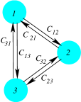
The necessary conditions for a permutation be a symmetry in directed weighted networks are of course much more restrictive than in the undirected unweighted case. For instance, the permutation $P_{(i,j)}$ discussed above will be a symmetry of the elementary Laplacian matrix $L_{(i,j)}$ only if the edge connecting the layers $i$ and $j$ were effectively undirected, i.e., $C_{ij}=C_{ij}^{T}=C_{ji}$. Nevertheless, this is not enough to assure that $P_{(i,j)}$ be a symmetry of the entire network. For instance, a permutation of the levels 1 and 2 in the block-network of Fig 6 would be a symmetry only if, besides of $C_{12}=C_{12}^{T}=C_{21}$, we have $C_{31}=C_{32}$ and $C_{13}=C_{23}$.

III.1 The results

We are now ready to state our main results. We have considered multilayer networks with the Laplacian matrix given by (43). The identical layers are generated by using the NetworkX NetworkX package for python, which allow us to build many types of random networks with prescribed topology and statistical properties. The connections between the layers are also randomly chosen with different statistical properties, mimicking in this way the situations where the inlayer and interlayer connection patterns evolve and are selected differently. The natural frequencies are draw according to the prescribed distributions, and the corresponding governing equations (3) and (4) are then solved with the help of the SciPy SciPy package for python.

Since all the layers in our network are identical, if the interlayer connection matrices $C_{ij}$ were diagonal, the corresponding interlayer connections will not contribute to the parameter ${\cal L}$ given by (II.1), which is precisely the quantity to be maximized in our optimization procedure. For these cases, one has ${\cal L}={\cal L}_{0}$, where ${\cal L}_{0}$ is the contribution to (II.1) from each isolated layer and, hence, the synchronization capability of the whole network is effectively the same of each isolated layer. In this case, one is not taking any advantage of the multilayer structure and, in this sense, this is the worst possible configuration for synchronization in these networks. However, starting with a multilayer network with diagonal interlayer connections, one may apply our algorithm only to the interlayer edges between two given layers and, in consequence, one will enhance considerably the network synchronization capability (increasing the value of ${\cal L}$, accordingly to the results of the Section II), whereas keeping the layers and the number of connections between them unchanged. This can be considered a minimal change in the network topology, but with a considerable impact on its synchronization capability. We will consider as optimal the network obtained from a full rewiring of the interlayer connections. Of course, one should expect a gradual improvement of the network synchronization capability by considering larger and larger rewiring ratio, but a more quantitative description of this process is still lacking.

We have performed exhaustive numerical simulations which have corroborated our main conclusions. Our analysis starts with a multilayer random network with diagonal interlayer connection, for which we construct a synchronization diagram $\langle r\rangle\times\lambda$ (see Fig. 7 for instance), where $\langle r\rangle$ corresponds to the average of the order parameter (5) evaluated on some time interval $\Delta t$

$$\langle r\rangle=\frac{1}{\Delta t}\int_{t_{0}}^{t_{0}+\Delta t}r(t)\,dt,$$ (45)

along the corresponding numerically integrated solutions of (1), starting with random initial conditions. The parameter $t_{0}$ is meant to be chosen in order to ensure the dissipation of any transient regime, and this can be monitored, for instance, from the standard deviation of $r$ on the integration interval. It is more convenient to work with the dimensionless evolution parameter $\tau=\alpha^{2}t$, which of course corresponds to set $\alpha=1$, and $\lambda=\lambda\alpha^{-2}$ and $\omega_{k}=\omega_{k}\alpha^{-2}$ in (1). It is clear that in this case we are invoking $\alpha^{-2}$ as the intrinsic time scale for our problem. For a fixed multilayer random network, one evaluates $\langle r\rangle$ for different values of $\lambda$ and depict the final diagram as a graphics $\langle r\rangle\times\lambda$. We then apply our algorithm for the interlayer connections, generating a new network, and repeat the same steps. By comparing the diagrams $\langle r\rangle\times\lambda$ of both networks, one can determine firmly which one has the best synchronization capabilities, and it always is the optimal non-diagonal case.

According to the discussions of the last Section, one should expect better results for sparse networks. Figs 7, 8, and 9

Figure 7: Synchronization diagram for a bilayer random network with 800 nodes disposed in two identical Barabasi-Albert layers, with 352 interlayer connections. (Interlayer connection probability $p=0.9$, see the text for details.) The oscillators native frequencies were drawn from a normal distribution with $\sigma\alpha^{-2}=1$. The entire network has average degree $\langle d_{k}\rangle=2.88$, and the minimal and maximal degrees are, respectively, 1 and 24. The synchronization threshold $\lambda_{c}\alpha^{-2}=0.81$, given by (30), is depicted as a vertical line. The red crosses corresponds to the original network with diagonal interlayer connections, for which ${\cal L}=2.11$, while the blue circles corresponds to a network with exactly the same layers, but with optimal interlayer connections, for which ${\cal L}=11.48$. The optimal network has, by construction, the same average degree, but the minimal and maximal degrees are now, respectively, 1 and 71. The curve and points at the bottom of the graphics correspond to the standard deviation associated with the average (45), which assures that the average $\langle r\rangle$ is being indeed evaluated in the stationary regime. It is clear from the diagram that the optimal non-diagonal interlayer connections has enhanced considerably the synchronization capability of the original network.

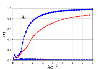
depict some typical cases built on Barabasi-Albert

Figure 8: Synchronization diagram, with the same conventions of Fig. 7, for a random network with 1200 nodes disposed in three identical Barabasi-Albert layers, with 192, 216, and 188 interlayer connections, corresponding to $p=0.5$. The trilayer network has average degree $\langle d_{k}\rangle=2.99$, synchronization threshold $\lambda_{c}\alpha^{-2}=0.78$, and the minimal and maximal degrees are, respectively, 1 and 55. The original network with diagonal interlayer connections (red crosses) has ${\cal L}=1.47$, while ${\cal L}=13.11$ for the optimal network (blue circles), for which the minimal and maximal degrees are, respectively, 1 and 74.

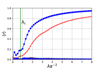
random networks barabasi1999 corresponding, respectively, to a bilayer, a trilayer, and a six-layer networks.

Figure 9: Synchronization diagram, with the same conventions of Fig. 7, for a random network with 2400 nodes disposed in six identical Barabasi-Albert layers, with 92, 104, 86, 104, 89, 106, 115, 83, 106, 108, 77, 100, 116, 85, 100 interlayer connections, corresponding to $p=0.25$. The six-layer network has average degree $\langle d_{k}\rangle=3.22$, synchronization threshold $\lambda_{c}\alpha^{-2}=0.72$, and the minimal and maximal degrees are, respectively, 1 and 42. The original network with diagonal interlayer connections (red crosses) has ${\cal L}=1.58$, while ${\cal L}=16.05$ for the optimal network (blue circles), for which the minimal and maximal degrees are, respectively, 1 and 58.

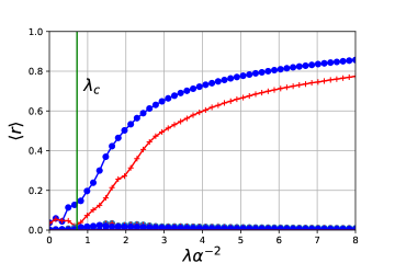
For all cases, one starts with a 400-nodes Barabasi-Albert network corresponding to the layers and, then, a multilayer network with diagonal interlayer connection is constructed. The interlayer connections are also random and the probability of two equivalent nodes in different layers be connected is given by $p$. We adopt for the bilayer, trilayer, and six-layer networks, respectively, $p=0.9$, $0.5$, and $0.25$. For all case, $\alpha^{2}t_{0}=4.25$ was enough to ensure the onset of the stationary regime and $\alpha^{2}\Delta t=0.75$ was used to evaluate $\langle r\rangle$ accordingly to (45). It is quite clear that the asymmetrical connection patterns systematically give rise to multilayer networks with far better synchronization capabilities.

IV Final remarks

In this paper, we have considered the synchronization problem for Stuart-Landau oscillators in random multilayer networks with identical layers. We have shown that the breaking of interlayer connection symmetries leads typically to an appreciable enhancement of the network synchronization capabilities, in the same spirit of Motter-Nishikawa phenomenon of asymmetry-induced synchronization (AISync) NishMotter . The dynamics of multilayer networks can be conveniently formulated in terms of effective block-networks, where a node stands for an entire layer of the original multilayer networkmulti1 ; multi2 . The presence of asymmetries in the interlayer connection patterns effectively transforms the problem into a directed block-network (see Fig. 6) which has typically far better synchronization capabilities than similar networks with symmetric interlayer connection pattern, which, on the other hand, are effectively described by undirected block-networks. Moreover, the most regular connection pattern, corresponding to diagonal interlayer connection matrices (see Fig. 1), is always the worst possible configuration for synchronization in these networks. In this sense, our results corroborate the main conclusions of ZhangNishMotter , namely that asymmetry-induced synchronization should be a rather generic property of structured networks. In fact, for unstructured networks with random frequency oscillators, symmetries should be extremely rare since, despite of preserving the connection topology, a node permutation must also preserve the oscillator native frequencies in order to be a genuine symmetry for the SL system. The problem of finding the symmetries of a SL system is equivalent to the so-called colored graph isomorphisms problem, which are indeed much more restrictive than the usual graph isomorphisms Nauty . In particular, if all the oscillators have different native frequencies, which is a quite common situation if the frequencies are assumed to be random real numbers, there will be no permutation symmetry for the system. In this sense, one should not expect in general an anti-correlation between symmetries and synchronization for unstructured random networks of oscillators mainly because one should not expect any symmetry for them.

Our multilayer random networks with identical layers are explicitly built in order to assure that some permutations of entire layers could in principle be genuine symmetries for the SL system. Since all the layers are identical, we have in this case $\boldsymbol{\omega}=P\boldsymbol{\omega}$, where $P$ is the pertinent entire-layer permutation matrix and $\boldsymbol{\omega}$ stands for the oscillator native frequencies vector for the whole network or, in other words, the oscillator native frequencies for the whole network are even under the action of $P$. However, a situation where a certain permutation $P$ preservers the Laplacian matrix, i.e. $[L,P]=0$, and the native frequencies are odd under its action, i.e. $\boldsymbol{\omega}=-P\boldsymbol{\omega}$, can be also considered a symmetry for the SL system (1), since under $P$ we will have a system such that $z_{k}\to\bar{z}_{k}$, which of course has the same synchronization properties. Such a system cannot have identical layers, in fact it must have layers with the same topology, but with reversed oscillator native frequencies. For these systems, the diagonal connection pattern is not anymore the worst possible case for synchronization, since the contribution from the interlayer edges to ${\cal L}$ does not vanish as for the even case, see (II.1). This kind of systems is quite interesting and would deserve a deeper analysis.

We would like also to recall that we opt in our analysis to keep the layers unchanged and to rewire the edges between then in order to optimize the synchronization. This could be considered a minimal change in the network topology, but typically with a considerable impact on its synchronization capability. This is not, however, the only optimization scheme one can envisage for the network. One could, for instance, to keep the edges unaltered and then to redistribute the oscillators native frequencies over the network. Let us suppose one keeps the layers identical in order to guarantee some possible permutation symmetries for the system. This problem can be formulated as follows: for a given Laplacian matrix $L$ in (19), which reordering of the vector $\boldsymbol{\omega}$ would lead to a maximal ${\cal L}$? It is clear from (19) that the maximum possible value for ${\cal L}$ corresponds to the situation where $\boldsymbol{\omega}$ is proportional to the eigenvector of $L$ with largest eigenvalue, say $\boldsymbol{\nu}_{\rm max}$, which, incidentally, is an optimal synchronization condition that has been already discovered numerically and by means of more intricate methods brede2008a ; buzna2009 ; kelly2011 ; skardal2014 . Hence, an optimal reordering of $\boldsymbol{\omega}$ would be that one which minimizes $\Gamma=\left|\boldsymbol{\omega}-\boldsymbol{\nu}_{\rm max}\right|$. However, this problem is much more complex computationally than the rewiring problem we have discussed in this paper. This issue is now also under investigation.

We finish by noticing that, despite of our results are indeed fully compatible with the conclusions of skardal2014 , in particular with the fact that anti-correlation between the frequencies of neighbor nodes favors synchronization (larger values of ${\cal L}$), the role played by the interlayer connection symmetries, as discussed in Section III, allows us to interpret our results as a genuine manifestation of the dynamical phenomenon of AISync in multilayer random networks with identical layers.

References

- (1) T. Nishikawa and A. E. Motter, Phys. Rev. Lett. 117, 114101 (2016). [arXiv:1608.05419]
- (2) Y. Zhang, T. Nishikawa, and A. E. Motter, Phys. Rev. E95, 062215 (2017). [arXiv:1705.07907]
- (3) Y. Zhang and A. E. Motter, Nonlinearity 31, R31 (2018). [1712.03245]
- (4) A. Arenas, A. Díaz-Guilera, J. Kurths, Y. Moreno, and C. Zhou, Phys. Rep. 469, 93 (2008).
- (5) A. Pikovsky, M. Rosenblum, and J. Kurths, Synchronization: A universal concept in nonlinear sciences, Cambridge University Press, 2003.
- (6) V. Nicosia, M. Valencia, M. Chavez, A. Diaz-Guilera, and V. Latora, Phys. Rev. Lett. 110, 174102 (2013).
- (7) L.M. Pecora, F. Sorrentino, A.M. Hagerstrom, T.E. Murphy, and R. Roy, Nature Commun. 5, 4079 (2014).
- (8) F. Sorrentino, L.M. Pecora, A.M. Hagerstrom, T.E. Murphy, and R. Roy, Sci. Adv. 2, e1501737 (2016).
- (9) Y.S. Cho, T. Nishikawa, and A.E. Motter, Phys. Rev. Lett. 119, 084101 (2017).
- (10) M. Kivela, A. Arenas, M. Barthelemy, J.P. Gleeson, Y. Moreno, and M.A. Porter, J. Complex Netw. 2, 203 (2014). [arXiv:1309.7233]
- (11) S. Boccaletti, G. Bianconi, R. Criado, C.I. del Genio, J. Gomez-Gardenes, M. Romance, I. Sendina-Nadal, Z. Wang, and M. Zanin, Phys. Rep. 544, 1 (2014). [arXiv:1407.0742]
- (12) R.S. Pinto and A. Saa, Phys. Rev. E92, 062801 (2015) [arXiv:1508.00518]
- (13) Y. Kuramoto, in Proceedings of the International Symposium on Mathematical Problems in Theoretical Physics, University of Kyoto, Japan, Lect. Notes in Physics 30, 420 (1975), edited by H. Araki.
- (14) S. H. Strogatz, Physica D 143, 1 (2000).
- (15) J. A. Acebrón, L. L. Bonilla, C. J. P. Vicente, F. Ritort and R. Spigler, Rev. Mod. Phys. 77, 137 (2005).
- (16) P.C. Matthews, R.E Mirollo, and S.H Strogatz, Physica D52, 293 (1991)
- (17) T. Aoyagi, Phys. Rev. Lett. 74, 4075 (1995). [arXiv:adap-org/9408001]
- (18) K. Ito and Y. Nishiura, Phys. Rev. E77, 036224 (2008)
- (19) E.M. Izhikevich, Dynamical Systems in Neuroscience: The Geometry of Excitability and Bursting, MIT Press (2007).
- (20) G. Gotwald, Chaos 25, 053111 (2015).
- (21) E. Ott and T. M. Antonsen, Chaos 18, 037113 (2008).
- (22) E. Ott and T. M. Antonsen, Chaos 19, 023117 (2009).
- (23) V. H. P. Louzada, N. A. M. Araujo, J. S. Andrade, Jr. and H. J. Herrmann, Sci. Rep. 2, 658 (2012).
- (24) P. Li, X. Sun, K. Zhang, J. Zhang and M. Small, Phys. Rev. E 88, 022817 (2013).
- (25) X. Zhang, Z. Ruan and Z. Liu, Chaos 23, 033135 (2013).
- (26) R.S. Pinto and A. Saa, Physica A 463, 87 (2016) [arXiv:1408.2483].
- (27) G. Filatrella, A. H. Nielsen, N. F. Pedersen, Eur. Phys. J. B. 61, 485 (2008).
- (28) A. E. Motter, S. A. Myers, M. Anghel, and T. Nishikawa, Nature Phys. 9, 191 (2013).
- (29) B. D. McKay and A. Piperno, J. Symb. Comp. 60, 94 (2013) [arXiv:1301.1493].
- (30) A.A. Hagberg, D.A. Schult and P.J. Swart, Exploring network structure, dynamics, and function using NetworkX, in Proceedings of the 7th Python in Science Conference (SciPy2008), G. Varoquaux, T. Vaught, and J. Millman (Eds), (Pasadena, CA USA), pp. 11-15, Aug 2008.
- (31) E. Jones, E. Oliphant, P. Peterson P, et al., SciPy: Open Source Scientific Tools for Python, 2001, http://www.scipy.org/ [Online; accessed 2014-08-10].
- (32) A. L. Barabasi, R. Albert, Science 286, 5439 (1999).
- (33) M. Brede, Phys. Lett. A 372, 2618 (2008).
- (34) L. Buzna, S. Lozano and A. Diaz-Guilera, Phys. Rev. E 80, 066120 (2009).
- (35) D. Kelly, G. A. Gottwald, Chaos 21, 025110 (2011).
- (36) P. S. Skardal, D. Taylor, and J. Sun, Phys. Rev. Lett. 113, 144101 (2014).