Implementation of mixed-dimensional models for flow in fractured porous media

Abstract

Models that involve coupled dynamics in a mixed-dimensional geometry are of increasing interest in several applications. Here, we describe the development of a simulation model for flow in fractured porous media, where the fractures and their intersections form a hierarchy of interacting subdomains. We discuss the implementation of a simulation framework, with an emphasis on reuse of existing discretization tools for mono-dimensional problems. The key ingredients are the representation of the mixed-dimensional geometry as a graph, which allows for convenient discretization and data storage, and a non-intrusive coupling of dimensions via boundary conditions and source terms. This approach is applicable for a wide class of mixed-dimensional problems. We show simulation results for a flow problem in a three-dimensional fracture geometry, applying both finite volume and virtual finite element discretizations.

1 Introduction

Simulation models for real-life applications commonly must represent objects with high aspect ratios embedded in the domains. This includes both objects of co-dimension 1, exemplified by fractures in a porous rock, and co-dimension 2 models such as reinforced concrete and root systems. Although the embedded objects occupy a small part of the simulation domain, they can have a decisive impact on the system behavior, thus their representation in the simulation model is critical. The small object sizes, and in particular the high aspect ratio, make an equi-dimensional representation computationally prohibitively expensive. The standard simulation technique has therefore been to apply homogenization to arrive at an, ideally, equivalent upscaled model. In recent years, advances in computational power, modeling approaches and numerical methods have made resolving the objects more feasible. This calls for the development of new simulation tools for mixed-dimensional problems that allow for a high degree of reuse of software designed for mono-dimensional simulations.

Here, we explore the implementation of a simulation model based on a newly developed modeling framework for flow and transport in fractured porous media [2, 1]. The model considers fractures as manifolds of co-dimension 1 that are embedded in the simulation domain, and further allows for intersections of fractures as objects of co-dimension 2 and 3. Central to our implementation is the representation of the mixed-dimensional problem as a graph, where the nodes represent mono-dimensional problems, and the edges represent couplings between subdomains. Discretization internal to each subdomain is then a matter of iterating over the nodes of the graph, and apply standard numerical methods by invoking, possibly legacy, mono-dimensional discretizations. Discretization of mixed-dimensional dynamics, which is commonly not handled by existing software, is associated with the edges of the graph. Depending on how the interactions are modeled, the implementation of the subdomain couplings comes down to treatment of boundary conditions and source terms, both of which are standard in most numerical tools.

Focusing on locally conservative methods, which are prevailing in porous media applications, we consider both virtual element and finite volume approaches for flow, in addition to finite volume techniques for transport. The simulation model discussed is implemented in the software framework PorePy [8], and is available at www.github.com/pmgbergen/porepy.

2 Mixed-dimensional flow in fractured porous media

Let us consider a $N$-dimensional domain $\Omega\subset\mathbb{R}^{N}$, typically $N=2$ or $3$, with outer boundary $\partial\Omega$. $\Omega$ represents the porous medium, which is composed of a $N$-dimensional domain $\Omega^{N}$ (the rock matrix) and lower-dimensional domains $\Omega^{N-1},\ldots,\Omega^{0}$, representing fractures and possibly objects of lower dimensions such as fracture intersections and intersections of fracture intersections. We assume that $\Omega^{d-1}\not\subset\Omega^{d}$ for $d=0,\ldots,N$, and $\Omega=\cup_{d}\Omega^{d}$. Let $\Gamma$ denote the set of internal boundaries between subdomains of different dimension. In each dimension, we consider the flow of a single-phase incompressible fluid, with governing equations stated on mixed form as

$$\vec{u}^{d}+\vec{K}\nabla p^{d} =0 \mathrm{in}\ \Omega^{d},d>0$$ (1)

$$\nabla\cdot\vec{u}^{d}-[\![\vec{u}^{d+1}\cdot\vec{n}^{d+1}]\!] =f^{d} \mathrm{in}\ \Omega^{d},d\leq N$$

$$\vec{u}^{d}\cdot{\vec{n}^{d}}+\kappa(p^{d-1}-p^{d}) =0 \mathrm{on}\ \Gamma.$$

The unknowns are the Darcy velocity $\vec{u}$ and the pressure $p$, and the data are the permeability ${K}$, the effective normal permeability $\kappa$ between the subdomains, and $f$ is sources and sinks. We define $\vec{u}^{N+1}=0$. The coupling between pairs of subdomains one dimension apart can be seen in the conservation statement, where the divergence of the flux in the dimension under consideration is balanced by source terms in the same dimension, and the contribution from the higher dimension via the jump $[\![\vec{u}^{d+1}\cdot\vec{n}^{d+1}]\!]$, which represent the net flux into the domain. From the higher dimension, this term will appear as the leakage into lower dimensions, which may be interpreted as an internal boundary. The last equation in (1) is a mixed-dimensional Darcy law with effective permeability $\kappa$, which models the flux between two subdomains separated by the interface $\Gamma$. On outer boundaries of each $\Omega^{d}$ we assign Dirichlet or Neumann conditions. For more details on the mathematical model, we refer to [9, 5, 7, 11, 3, 2, 12, 4]. We also note that a similar model can be used to express transport of a scalar in mixed-dimensional geometries, see [6].

3 Discretization of mixed-dimensional problems

To device design principles for an implementation of the model (1), we first observe that interaction between subdomains takes the form of boundary conditions from lower to higher dimension and source terms. Moreover, this should apply also for more general classes of models, including most, if not all, that are built upon conservation principles [1]. Thus a versatile implementation should be based on independent discretizations on the subdomains, together with appropriate coupling conditions. Below we describe how this is naturally achieved by representing the computational grid as a graph, and discretization as an iteration over its nodes and edges. This abstraction allows for reuse of an existing code base, and if combined with a flexible interface between the grids, it can be extended to heterogeneous discretizations and multi-physics modeling.

In Subsection 3.1 we present the grid structure needed for the mixed-dimensional description of (1), while in Subsection 3.2 we briefly introduce the numerical discretizations.

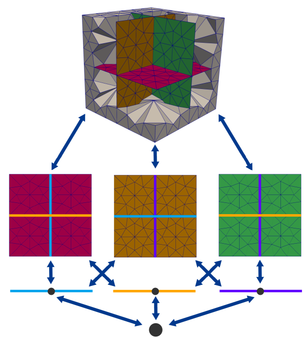
Figure 1: Hierarchy of grids derived from the meeting of three 2D objects embedded in 3D space. The mixed-dimensional grid is naturally represented as a graph, with individual grids forming nodes.

Figure 2: Structure of linear system resulting from a discretization of the mixed-dimensional problem on the geometry shown in Figure 1. The diagonal blocks represent the discretization of each grid, while the off diagonal blocks represent the interface condition between two and two grids. The top and bottom colors of each coupling block correspond to the higher and lower dimensional grids, respectively.

3.1 Grid structure

For simplicity, we require that the computational mesh is fully conforming to all objects $\Omega^{d}$ in all dimensions. This condition can be relaxed, e.g. by applying mortar discretizations in the transition between subdomains, however, we will not pursue this herein.

To illustrate the mixed-dimensional grid structure, we consider the hierarchy of grids depicted in Figure 1. The main domain is $\Omega=[-1,1]^{3}$. Define the fracture $\Omega_{1}^{2}=[-1,1]\times[-1,1]\times\{0\}$, and similarly let $\Omega_{2}^{2}$ and $\Omega_{3}^{2}$ be embedded in the $xz$ and $yz$ plane, respectively. The intersection between pairs of fractures defines intersection lines $\Omega_{i}^{1},i=\{1,2,3\}$ along the coordinate axes. Further, the intersection lines intersect to define $\Omega^{0}$ in the origin. Finally, define $\Omega^{3}=\Omega\setminus\big{(}\bigcup_{d={0,1,2}}\bigcup_{i}\Omega_{i}^{d}\big{)}$.

To apply a discretization scheme on this grid structure requires iterations over all subdomains and their connections. This is readily implemented by considering the subdomains as nodes in a graph, with the connections forming edges, as illustrated in Figure 1. We define $nodes(\cdot)$ as a function such that given a dimension $d$ it returns the nodes in the graph of the same dimension. Similarly, $edges(\cdot,\cdot)$ is a function that, given consecutive dimensions $d$ and $d-1$, returns the edges in the graph associated with nodes of dimension $d$ and $d-1$. This abstraction is particularly suitable for existing software frameworks that can handle grids of a single but flexible dimension. Discretization of a mixed-dimensional problem can then be defined by two iterations; (i) an iteration on the nodes of the graph to invoke the standard solver on each subdomain, and (ii) an iteration on the edges of the graph to impose coupling conditions on subdomain boundaries.

Given a suitable numerical scheme for the discretization of (1), the system obtained from the first iteration gives the following block-diagonal matrix

$${\rm diag}(A^{N},A^{N-1},\ldots,A^{1},0),$$

where $A^{d}$ is related to the set $nodes(d)$ of nodes in the graph. The matrices $A^{d}$ are block diagonal, with one block for each node defining the mono-dimensional discretization of each sub-grid. The interface conditions between $d$ and $d-1$ can be written as

$$\begin{bmatrix}H^{d,d-1}&C^{d,d-1}\\ C^{d,d-1}&L^{d,d-1}\end{bmatrix}$$

where the matrices $C^{d,d}$ and $C^{d-1,d-1}$ are contributions of the coupling condition for the higher and lower dimension, both having a block diagonal structure. The matrix $C^{d,d-1}$ represents the inter-dimensional contribution and has a block structure. All three matrices contain one block for each edge in $edges(d,d-1)$. For a three-dimensional problem, the general structure of the global matrix is

$$\begin{bmatrix}A^{3}+H^{3,2}&C^{3,2}&0&0\\ C^{3,2}&A^{2}+L^{3,2}+H^{2,1}&C^{2,1}&0\\ 0&C^{2,1}&A^{1}+L^{2,1}+H^{1,0}&C^{1,0}\\ 0&0&C^{1,0}&L^{1,0}\\ \end{bmatrix}.$$

The matrix in Figure 2 illustrates the block structure associated with the mesh of Figure 1.

3.2 Conservative discretizations

We consider two discretization schemes for the mixed-dimensional pressure equation (1). The simplest option is a finite volume scheme built as a two-point flux approximation (TPFA), which is standard in commercial porous media simulators. This scheme is easy to implement, and, with the data structures outlined above, a simple extension to mixed-dimensional problems is fairly straightforward; more complex approaches involving mortar variables are currently under investigation. However, TPFA is consistent only for K-orthogonal grids, and can be expected to suffer from poor accuracy for the complex grids needed to cover realistic fracture networks. Our second approach applies the dual form of the virtual element method [10], with the extension to mixed-dimensional problems, as discussed in [6]. The virtual element method puts almost no restrictions on the cell shape, and is thus ideally suited for handling rough grids. This also makes it possible to merge simplex cells into general polyhedral shapes, and thus reduce the number of degrees of freedom. We do not consider non-simplex cells here, see [6] for details.

Given a flux field, the extension of the tracer advection problem using a first-order upwind scheme is equivalent to the procedure above.

4 Example simulation

In this part we present an example to assess the above models and numerical schemes. The source code of the example is available online in the PorePy repository.

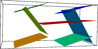
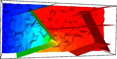
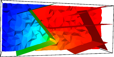
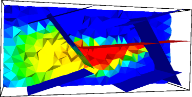
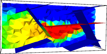
Figure 3: Top: representation of the considered geometry for the example. Centre: pressure field for the TPFA (left) and VEM (right). Bottom: concentration at the final time with the discharge computed by the TPFA and VEM. The flow is from the right to the left. In all the figures a “Blue to Red Rainbow” colour map is used in the range $[0,1]$.

We consider a 3D fracture network with heterogeneous permeabilities in the fractures and on their intersections exploiting the mixed-dimensional structure of the model. The domain is $\Omega=[0,2]\times[0,1]\times[0,1]$ and the geometry of the network, containing 7 fractures, is depicted at the top of Figure 3. The permeability in the rock matrix is assumed unitary. The fracture marked with a red color in the figure is high permeable with permeability equal to $10^{4}$, while the other fractures behave as barriers having permeabilities equal to $10^{-4}$. The fracture aperture is constant and equal to $10^{-2}$ for all fractures. All 1D intersections inherit the highest permeability of the intersecting fractures. Thus, the ones involving the highly permeable fracture are permeable, and the others behave as impermeable paths. The grid is composed by 23325 tetrahedra for the 3d rock matrix, 2624 triangles for the fractures, and 48 segments for the fracture intersections.

We impose a pressure gradient by setting the pressure on the left boundary to 0 and the right boundary to 1. The other boundaries are given a zero flux condition. We compute the pressure field and the discharge (flux) using the TPFA and VEM on the same grid. The discharge is a face variable, obtained by back-calculation from the pressures in the TPFA method and directly computed for the VEM. The computed solution is represented in the middle row of Figure 3. The low permeable fractures at the right end of the domain do not affect the pressure field much, as the conductive fracture makes a high permeable connection between the right and the center part of the domain. However, at the left part the low permeable fractures force a pressure gradient between the small gap between two of the fractures (orange and green). The solutions obtained from both methods are in good agreement.

Once the discharge is computed we consider a pure transport problem, where the advective field is given by the discharge. We inject a tracer with concentration 1 on the right part of the domain with outflow on the left part. The tracer thus follows the discharge, flowing in the high permeable fracture first and then propagating in the rock matrix, avoiding the low permeable fractures in the left part of the domain. An implicit Euler scheme is applied for the time discretization with time step equal to $0.01$. The final time of the simulation is $3$. As in the case of the pressures, the tracer solutions for the discharge computed by the TPFA or by the VEM are in agreement.

5 Concluding remarks

We have discussed the design of simulation tools for mixed-dimensional equations, in the setting of flow in fractured porous media. We presented a data hierarchy where the mixed-dimensional structure is a graph, with each node representing a standard mono-dimensional domain. This allows for extensive reuse of existing code designed for mono-dimensional problems, and also facilitates simple implementation of new discretization schemes. Numerical examples of flow and transport in a three-dimensional fractured medium illustrate the capabilities of a simulation tool based on this approach.

References

- [1] W. M. Boon, J. M. Nordbotten, and J. E. Vatne, Mixed-dimensional elliptic partial differential equations, arXiv:1710.00556, 2017.
- [2] W. M. Boon, J. M. Nordbotten, and I. Yotov, Robust discretization of flow in fractured porous media, Tech. report, arXiv:1601.06977v2, 2017.
- [3] K. Brenner, J. Hennicker, R. Masson, and P. Samier, Gradient discretization of hybrid-dimensional Darcy flow in fractured porous media with discontinuous pressures at matrix-fracture interfaces, IMA Journal of Numerical Analysis (2016).
- [4] F. A. Chave, D. Di Pietro, and L. Formaggia, A Hybrid High-Order method for Darcy flows in fractured porous media, Tech. report, HAL archives, 2017.
- [5] C. D’Angelo and A. Scotti, A mixed finite element method for Darcy flow in fractured porous media with non-matching grids, Mathematical Modelling and Numerical Analysis 46:02 (2012), 465–489.
- [6] A. Fumagalli and E. Keilegavlen, Dual virtual element methods for discrete fracture matrix models, arXiv:1711.01818, 2017.
- [7] A. Fumagalli and A. Scotti, An Efficient XFEM Approximation of Darcy Flows in Arbitrarily Fractured Porous Media, Oil and Gas Sciences and Technologies - Revue d’IFP Energies Nouvelles 69:4 (2014), 555–564.
- [8] E. Keilegavlen, A. Fumagalli, R. Berge, I. Stefansson, and I. Berre, Porepy: An open source simulation tool for flow and transport in deformable fractured rocks, arXiv:1712.00460, 2017, In preparation for Computer & Geosciences.
- [9] V. Martin, J. Jaffré, and J. E. Roberts, Modeling Fractures and Barriers as Interfaces for Flow in Porous Media, SIAM J. Sci. Comput. 26:5 (2005), 1667–1691.
- [10] L. Beirão da Veiga, F. Brezzi, L. D. Marini, and A. Russo, Mixed virtual element methods for general second order elliptic problems on polygonal meshes, ESAIM: M2AN 50:3 (2016), 727–747.
- [11] N. Schwenck, B. Flemisch, R. Helmig, and B. Wohlmuth, Dimensionally reduced flow models in fractured porous media: crossings and boundaries, Computational Geosciences 19:6 (2015), 1219–1230 (English).
- [12] A. Scotti, L. Formaggia, and F. Sottocasa, Analysis of a mimetic finite difference approximation of flows in fractured porous media, ESAIM: M2AN (2017).