The ESO’s VLT Type Ia supernova spectral set of the final two years of SNLS ^,

Abstract

Aims. We aim to present 70 spectra of 68 new high-redshift type Ia supernovae (SNe Ia) measured at ESO’s VLT during the final two years of operation (2006-2008) of the Supernova Legacy Survey (SNLS). This new sample complements the VLT three year spectral set. Altogether, these two data sets form the five year sample of SNLS SN Ia spectra measured at the VLT on which the final SNLS cosmological analysis will partly be based. In the redshift range considered, this sample is unique in terms of homogeneity and number of spectra. We use it to investigate the possibility of a spectral evolution of SNe Ia populations with redshift as well as SNe Ia spectral properties as a function of lightcurve fit parameters and the mass of the host-galaxy.

Methods. Reduction and extraction are based on both IRAF standard tasks and our own reduction pipeline. Redshifts are estimated from host-galaxy lines whenever possible or alternatively from supernova features. We used the spectro-photometric SN Ia model SALT2 combined with a set of galaxy templates that model the host-galaxy contamination to assess the type Ia nature of the candidates.

Results. We identify 68 new SNe Ia with redshift ranging from $z=0.207$ to $z=0.98$ for an average redshift of $z=0.62$. Each spectrum is presented individually along with its best-fit SALT2 model. Adding this new sample to the three year VLT sample of SNLS, the final dataset contains 209 spectra corresponding to 192 SNe Ia identified at the VLT. We also publish the redshifts of other candidates (host galaxies or other transients) whose spectra were obtained at the same time as the spectra of live SNe Ia. This list provides a new redshift catalog useful for upcoming galaxy surveys. Using the full VLT SNe Ia sample, we build composite spectra around maximum light with cuts in color, the lightcurve shape parameter (’stretch’), host-galaxy mass and redshift. We find that high-$z$ SNe Ia are bluer, brighter and have weaker intermediate mass element absorption lines than their low-$z$ counterparts at a level consistent with what is expected from selection effects. We also find a flux excess in the range [3000-3400] Å for SNe Ia in low mass host-galaxies ($M<10^{10}M_{\odot}$) or with locally blue $U-V$ colors, and suggest that the UV flux (or local color) may be used in future cosmological studies as a third standardization parameter in addition to stretch and color.

1 Introduction

The use of type Ia supernovae (SNe Ia) as standardisable candles has led to the discovery of the acceleration of the universal expansion (Perlmutter et al. 1997, 1999; Riess et al. 1998; Schmidt et al. 1998). This acceleration is usually attributed to a dark energy (DE) component that contributes  70% of the energy budget of the Universe. Characterizing the nature of this component by constraining its equation-of-state parameter $w$ (the DE pressure to energy density ratio) has become a major goal of observational cosmology. For this purpose, a combination of various probes has been used. Among those probes, the measurement of luminosity distances to SNe Ia provides the simplest and most direct way of probing DE at low to intermediate redshifts (Astier et al. 2006; Wood-Vasey et al. 2007; Kowalski et al. 2008; Sullivan et al. 2011; Suzuki et al. 2012; Campbell et al. 2013; Rest et al. 2014; Betoule et al. 2014).

Since the original Supernova Cosmology Project and High-z team projects, new generations of observational programs have been developed in order to fill the gaps in the Hubble diagram. Among those, the Supernova Legacy Survey (SNLS), with its 427 spectroscopically confirmed SNe Ia in the range $0.15<z<1.1$, is the largest supernova survey at high redshift to date.

SNLS was a five year experiment conducted as part of the Deep Survey of the Canada-France-Hawaii Telescope Legacy Survey (Sullivan et al. 2003). It is a spectro-photometric program aiming at discovering and following SNe Ia at intermediate to high redshifts. Conducted from mid-2003 to late 2008, the experiment was split into two surveys. A photometric program at the Canada-France-Hawaii Telescope (CFHT) implemented a rolling search technique that permitted the detection of new SN Ia candidates as well as the follow-up of their lightcurves in several photometric bands (mainly MegaCam $g_{M}$, $r_{M}$, $i_{M}$ and $z_{M}$; Boulade et al. 2003). Over the five years of operation, around 1000 SN Ia candidates with well sampled multi-band lightcurves were obtained (Guy et al. 2010; Bazin et al. 2011). SNLS spectroscopic follow-up programs have been performed in parallel on 8-10 meter diameter telescopes to secure the candidate type and redshift. Spectra of about half of the SNLS SNe Ia have been acquired at the ESO Very Large Telescope (VLT), while the remaining spectra have been obtained at the Gemini-North and South, Keck I and II telescopes.

Astier et al. (2006) published the first SNLS cosmological analysis based on the first year data set consisting of 71 SNe Ia measured from August 2003 to July 2004. Photometry calibration and luminosity distances to 252 SNe Ia measured in the first three years of operation were presented in Regnault et al. (2009) and Guy et al. (2010), respectively. The corresponding spectra and redshifts were published in Howell et al. (2005); Bronder et al. (2008); Balland et al. (2009); Walker et al. (2011). Combining the SNLS three year SNe Ia with low-redshift (z¡0.1) SNe Ia from the literature (Hicken et al. 2009; Contreras et al. 2010), intermediate redshift SNe Ia from the 1st year of Sloan Digital Sky Survey SDSS-II Supernova Survey (Holtzman et al. 2008; Kessler et al. 2009) and a dozen high-redshift SNe Ia from the Hubble Space Telescope (HST) (Riess et al. 2007), Conley et al. (2011) produced the most advanced supernova Hubble diagram at the time, with 472 SNe Ia in total. More recently, based on an combined flux calibration of SNLS and SDSS (Betoule et al. 2013), Betoule et al. (2014) performed a joint analysis of SNLS and SDSS-II supernova sets (the Joint Lightcurve Analysis – JLA). Including external, non-SN datasets in their cosmological analysis, such as the CMB measurements from the Planck (Planck collaboration XV 2013) and WMAP experiments (Bennett et al. 2013), and the Baryon Acoustic Oscillation (BAO) results (Beutler et al. 2011; Padmanabhan et al. 2012; Anderson et al. 2012), Betoule et al. (2014) obtain a value of the equation of state $w=-1.028\pm 0.055$ (including both systematics and statistical uncertainties, assuming a flat universe), the most precise measurement to date (see Aubourg et al. 2015; Alam et al. 2017 for recent constraints with similar precision based on BAO scale measurements from the Baryon Oscillation Spectroscopic Survey (BOSS) experiment).

The present paper focuses on the description and analysis of SNLS spectra taken at the VLT between August 2006 and September 2008 (the final two years of SNLS). It complements the analysis of the first three years SNLS-VLT spectra published in Balland et al. (2009). Confirmed SNe Ia of the new sample having sufficient photometric information will be included in the SNLS 5yr Hubble diagram (Betoule et al. 2017, in prep). Also published in this paper are the redshifts of other objects (host galaxies or other transients) whose spectra were obtained at the same time as the spectra of live SNe Ia through the use of the multi-object spectroscopic (MOS) mode of the FORS instruments at the VLT. This list provides a new redshift catalog useful for upcoming galaxy surveys.

Spectroscopy is essential not only for securing the type and redshift of the SN Ia candidates, but also because SNe Ia spectra are a rich source of physical information about their explosion conditions and composition. Even though the signal-to-noise ($S/N$) ratio of SNLS spectra is not ideal for detailed analyses, and despite the fact that they are usually only obtained at a single phase (most often around maximum light), they have been used in several studies that search for empirical correlations beetwen SNe Ia peak luminosity and spectroscopic features in order to reduce the residual dispersion in the Hubble diagram. Bronder et al. (2008) and Walker et al. (2011), using SNLS spectra and low-redshift spectra compiled from the literature, show the existence of a significant correlation between Hubble residuals and the equivalent width of Si ii ($\sim$ 4130 Å) and Mg ii ($\sim$ 4300 Å) absorptions, even though not at the level of the correlations of Hubble residuals with photometric color and stretch used in the standardization process. In the same spirit, using spectra of SNe Ia at low and higher redshift, Nordin et al. (2011) find a correlation between the SALT2 color and the pseudo-equivalent width of Si ii$\lambda 4130$ that could be used to improve cosmological distance measurements with SNe Ia roughly at the level obtained by the usual standardization procedure based on lightcurve shape and color parameters. (We note, however, that this effect is not seen by Chotard et al. 2011). More recently, Milne et al. (2015) use SNLS-VLT three year spectra, among others, to explore the spectral region producing UV/optical color differences seen in SNe Ia populations.

Underlying cosmological analyses with SNe Ia, the hypothesis that SNe Ia properties do not evolve with redshift statistically in a way that is not corrected for by the usual stretch- and color-luminosity correction, can be assessed with spectral data. Foley et al. (2008a), using various SNe Ia samples from Lick and Keck observatories and from the ESSENCE program (Wood-Vasey et al. 2007), make a comparison of composite spectra at low and high redshift and show that once galaxy light contamination is accounted for, the two samples are remarkably similar. Although several minor localized deviations between the low and high-redshift spectra are found, the difference constrains the evolution of SN spectral features to be less than 10% in relative flux in the optical rest-frame. Using the SNLS three year sample, Balland et al. (2009) compute a composite spectrum around maximum light at $z>0.5$ and compare it with its lower redshift counterpart. Absorption features due to intermediate mass elements (IME) around 4000 Å are found to be shallower in the high redshift spectrum. This is consistent with the SNe Ia observed at higher redshift being more luminous, hence displaying hotter ejecta with a higher ionization level than at low redshift (Sullivan et al. 2009). Comparing SNe Ia spectra obtained with the Hubble Space Telescope Imaging Spectrograph (HST-STIS) with ground-based counterparts with similar stretches and phases, Cooke et al. (2011) find a similar trend in the UV region of the spectra. They interpret these discrepancies as representing compositional variations among their sample rather than being due to an evolutionary effect. Maguire et al. (2012) improve over the Cooke et al. (2011) analysis by using 32 low redshift ($0.001<z<0.08$) SNe Ia HST-STIS spectra and compare them to the sample of Ellis et al. (2008). They find that their mean low redshift near-UV spectrum has a depressed flux compared to its intermediate redshift counterpart, consistent with evolution of the near-UV continum at the 3$\sigma$ level. This is in qualitative agreement with Foley et al. (2012) who compare a sample of 17 Keck/SDSS high-quality spectra at intermediate redshift to a low-redshift sample with otherwise similar properties: the Keck/SDSS SNe Ia have, on average, extremely similar rest-frame optical spectra, but a UV flux excess with respect to the low redshift sample. In this paper, we reassess the issue of supernova evolution with redshift in the light of our new sample. We also look for spectral differences arising from splitting our sample by stretch or host-galaxy mass that go beyond mere selection effects.

We describe the SNLS photometric survey and spectroscopic programs in Sect. 2. In Sect. 3, we present the acquisition and reduction of our new spectral data. We present our redshift estimate and SN Ia identification procedures in Sect. 4. Results on individual SN Ia spectra are presented in Sect. 5, as well the redshift catalog of other, non-SNe Ia. The average properties of our SN Ia sample is discussed in Sect. 6. A comparison with the VLT three year sample is also provided in that section. In Sect. 7, we build composite spectra below and above $z=0.6$ (the average redshift of our sample) and discuss their differences in the context of a possible redshift evolution of SNe Ia spectral properties. We also study spectral differences arising from splitting our sample by stretch or host-galaxy stellar mass. We discuss our findings and draw our conclusions in Sects. 8 and 9.

2 The SNLS experiment

2.1 The photometric survey

The SNLS survey is a Stage II Dark Energy experiment (Albrecht et al. 2006) aiming at constraining the DE equation of state parameter at the 10 percent level using several hundreds of precisely calibrated SNe Ia lightcurves sampled around the B-band maximum luminosity. Detection and photometric follow-up are made through an optical imaging survey using the MegaCam camera on the 3.6m CFHT in Hawaii (Boulade et al. 2003). The supernova candidates are detected thanks to their time-varying luminosity in relation to a reference image in four 1 square degree fields (D1-D4) with low Galactic-extinction. The fields have been observed every 3-5 nights (2-4 days in supernova restframe) during 5 to 6 lunations per year. This rolling search technique permits simultaneous observations of a large number of SN Ia candidates and the construction of multi-color lightcurves over time.

2.2 The spectroscopic surveys

Spectroscopic follow-up is necessary to assess the SN Ia nature of the candidates and estimate their redshift. Due to the faintness of distant SNe Ia ($r_{M}\sim 24$ at $z\sim 1$), the spectroscopic follow-up is done with 8-10 meter class telescopes. Two large programs at the VLT were allocated a total of 500h of observing time during the first four years of SNLS. A similar amount of time was allocated on the Gemini North and South telescopes. On the Keck I and II telescopes, about four nights per semester were allocated to SN followup during the five years of SNLS. Candidates were selected for spectroscopy based on the quality of the first few measured photometric points on their lightcurves (Sullivan et al. 2006a). Spectra of 755 candidates have been measured, amounting to roughly half of the photometric SN Ia candidates.

High redshift candidates ($z>0.6$) were preferentially observed by the Gemini telescopes because of the improved sky lines subtraction with the nod-and-shuffle mode available at these telescopes (Glazebrook & Bland-Hawthorn 2001). More than 200 candidates were observed on Gemini from August 2003 to May 2008, 150 of which have been identified as SNe Ia (Howell et al. 2005; Bronder et al. 2008; Walker et al. 2011).

Lower redshift targets were usually observed at the VLT using the visual and near UV spectrographs FORS1 and FORS2 (Appenzeller et al. 1998). Roughly 50% of the SNLS spectra (321 out of 755) were obtained during the two VLT large programs (European Southern Observatory Large Programs 171.A-0486 and 176.A-0589) from June 2003 to September 2007. 124 objects, observed between June 2003 and July 2006, have been identified as SNe Ia (either SN Ia  or SN Ia$\star$, see our classification Sect. 4.3). SNe Ia measured in long-slit spectroscopy mode (LSS) during this period constitute the VLT three year SN Ia data set from SNLS (Balland et al. 2009). This set is supplemented by 59 SNe Ia observed from August 2006 until September 2007 and published in the present paper. We also add to the present sample 8 SNe Ia  that were measured in MOS mode during the first 3 years of SNLS but not published in Balland et al. (2009) and one that was identified as a SN Ia  by Bazin et al. (2011) after a new extraction (see Sect. 3.1). In total, the sample presented in this paper thus contains 68 SNe Ia (see Sect. 3) whose redshift ranges from 0.21 to 0.98. Besides SNe Ia, 28 SN II, 9 SN Ib/Ic and 12 AGN were identified in the full VLT spectral sample. Finally, the identification was inconclusive for 89 (27%) candidates.

Several dozen candidates were observed at the Keck telescopes, in particular objects in the northernmost SNLS field (D3) that was not observable from the VLT. Around 150 SNLS candidate observations have been performed at Keck. A subset of these Keck spectra with a substantially higher $S/N$ than needed purely for typing are presented in Ellis et al. (2008).

3 The SNe Ia spectral set

3.1 The SN Ia sample

The SNe Ia sample (SN Ia  and SN Ia$\star$) of the present analysis contains the SNe Ia spectra observed at VLT during the last year and a half of the SNLS survey, namely from August, 1st 2006 up to the end of the survey mid-2008. As mentioned above, we also publish the spectra of SN 05D1dx, SN 05D1hm, SN 05D1if, SN 05D2le, SN 06D2ag, SN 06D4ba, SN 06D4bo and SN 06D4bw that were acquired in MOS mode before August, 1st 2006 but were not included in the three year VLT spectral sample (Balland et al. 2009) as the extraction pipeline used for that analysis did not support MOS mode. For completeness, we further add the spectrum of SN 06D2bo, a Type Ia supernova measured in LSS mode in February 2006 that was first misclassified as a non-SN Ia object, then reclassified by Bazin et al. (2011). Altogether, 107 spectra of 104 candidates have been analyzed in the present study, 68 of which are identified as SNe Ia (see Sect. 5).

3.2 Data acquisition and reduction

Up until the beginning of September 2005, all the real-time spectroscopic follow-up with FORS1 and FORS2 was done in long slit mode. By that time, SNLS had been running for slightly more than two years and was starting to accumulate a significant number of transients that lacked real-time spectroscopic follow-up. From September 2005 onward we used the multi-object spectroscopic (MOS) mode of FORS1 and FORS2 to target live transients, the host-galaxy of any other transient that happened to be within the FORS2 field of view and randomly selected field galaxies (see Sect. 5.4).

The MOS mode consists of 38 movable blades that can be used to make 19 slits anywhere in the FORS focal plane. The advantage of the MOS mode over precut masks (the MXU mode) is that it allows one to configure the focal plane in a very short amount of time. The MXU masks require at least one day to manufacture and need to be inserted into the FORS mask exchange unit during the afternoon, which means that there is some delay in targeting the live transient. Furthermore, the MXU mode is available with FORS2 only. The disadvantage of the MOS mode is that the length of the slits are fixed – the slit lengths vary between 20″ (even numbered slits) and 22″ (odd numbered slits). With respect to the MXU mode, this reduces the flexibility one has in selecting targets, and it usually means that only one object (generally the SN) is observed in the center of the slit (length wise). Some objects are observed close to the slit ends, which complicates the processing of the data.

We used one of two setups with FORS. If the SN was likely to be below $z\sim 0.7$, we used the 300V grism with the GG435 order sorting filter. If it was likely to be at a higher redshift we used the 300I grism with the OG590 order sorting filter. The slit widths were set to 1″. For all observations, we used the atmospheric dispersion corrector (ADC) and set the position angle to pass through the SN and the center of its host-galaxy. The FORS data were reduced using a mixture of standard IRAF tasks and our own routines that were specifically written to process MOS data from FORS1 and FORS2. Each spectrum was calibrated in wavelength and flux. For the purpose of flux calibration, we produced a number of calibration curves from the observation of spectro-photometric standard stars and updated them periodically for a given setup. Differential slit losses were partially corrected by the ADC. Residual losses were taken into account with the recalibration procedure described in Sect. 4.3. No correction of telluric features was performed. For the SNe, we also computed an error spectrum derived from Poisson noise in regions of the 2D sky-subtracted spectrum that are free of objects.

4 Spectral analysis

4.1 Redshift estimates from host-galaxy lines ($z_{host}$)

Redshifts are estimated from strong spectral features when present and are not corrected to the heliocentric reference frame. The most commonly identified host-galaxy features in the spectra are emission lines from the [O ii] unresolved $\lambda\lambda$3727, 3729 doublet, H$\beta$ $\lambda$4861, the [O iii] doublet $\lambda\lambda$4959,5007, H$\alpha$ $\lambda 6563$ and absorption lines from higher order Balmer transitions, and Ca ii H&K $\lambda\lambda$3934, 3968. In some spectra, other host-galaxy lines such as [Ne iii] $\lambda$3869, [N ii] $\lambda$6549, [N ii] $\lambda$6583 and [S ii] $\lambda\lambda$6716, 6730 are identified. To estimate the redshift, we perform a gaussian fit of each identified host-galaxy emission or absorption line. Where possible, we preferentially use well defined host-galaxy features located in the center of the spectral range. We assign an error of $\delta z\sim 0.001$ on the redshift derived from the host-galaxy lines width, typical of the uncertainty obtained on host-galaxy redshifts (Lidman et al. 2005; Hook et al. 2005; Howell et al. 2005; Balland et al. 2006, 2007; Baumont et al. 2008). About 75% of the redshifts of our sample come from host-galaxy spectral lines, the remaining 25% come from SN features, because of insufficient or nonexistent host-galaxy signal in the spectra.

4.2 Redshift estimates from SN features $(z_{SN}$)

If there is no apparent host-galaxy line, the redshift is estimated from the supernova features themselves. First, a rough estimate is visually inferred from one of the large troughs characteristic of SN Ia  spectra (e.g., Ca ii or Si ii $\lambda$4130). Then, we perform a combined fit of the observed lightcurves and spectrum of the object using SALT2 (Guy et al. 2007, see Sect. 4.3 below) over a grid of redshift values regularly spaced around the input value, with a step of $\Delta z=0.005$. The redshift value is given by the best-fit $\chi^{2}$. As the supernova features have widths larger than those of host-galaxy lines, we assign an error of $\delta z\sim 0.01$ on the supernova redshifts and we consider this value as typical of the error obtained from SN features. Indeed, the distribution of $z_{SN}-z_{host}$ computed on a subset of candidates for which both redshifts are available has a mean of -0.001 and a standard deviation $\sigma\sim 0.007$. This supports the value of 0.01 adopted as a typical error for $z_{SN}$. In 20% of cases, the best-fit redshift is further refined by visual inspection of the spectral fit, that is, the redshift is slightly shifted from the best-fit value to visually ensure the best overall agreement between the model and the spectrum. These cases usually correspond to noisy spectra with $S/N$ per wavelength bin $\lesssim 1$ and a high $\gtrsim 40$ % fraction of host galaxy contamination. As an independent check, we also use SNID (Blondin & Tonry 2007; Blondin et al. 2011) to secure our estimates.

4.3 SN identification

To assess the Ia nature of the candidates, we follow the procedure described in Baumont et al. (2008) and extensively used in Balland et al. (2009). We perform a combined fit of observed lightcurves and spectra with SALT2 using a $\chi^{2}$ minization procedure. Telluric absorptions present in the spectra are masked. A galaxy component modeling the host-galaxy is added to the SN model to take into account host-galaxy contamination. The overall fraction of the host-galaxy in the full model is a free parameter that is adjusted during the fit. Host-galaxy models include PEGASE2 synthetic templates (Fioc & Rocca-Volmerange 1997, 1999) for elliptical (E), lenticular (S0), Sa, Sb, Sc and Sd Hubble types at various ages. We also consider Kinney et al. (1996) templates for the same types, excluding Sc and Sd. The best-fit host-galaxy model is obtained by interpolation between two contiguous types in the Kinney template sequence or two contiguous galaxy ages in the PEGASE2 templates (see Baumont et al. 2008; Balland et al. 2009 for more details). The final supernova spectrum is obtained by subtracting the best fit host-galaxy model from the full spectrum. We do not add host-galaxy lines to the PEGASE2 templates and, consequently, line residuals often contaminate the final SN spectrum. This does not impact the identification of the candidate type as these residuals are localized and do not affect the overall spectral shape.

The best-fit SALT2 model is characterized by a SN color $c$ (defined as a color excess: $c$ is the $B-V$ color of the candidate at maximum light minus the average color of the SALT2 training sample supernovae), a lightcurve width parameter $x_{1}$ linked to the stretch $s$ (a $s=1$ SN Ia  has $x_{1}=0$), the MJD date of B-band maximum light and an overall normalization parameter $x_{0}$ . Imperfect flux calibration of the candidate spectrum is taken into account by allowing the photometric model to be recalibrated (twisted) to fit the spectrum using a recalibration function parametrized as $\exp(\sum\gamma_{i}{\tilde{\lambda}}^{i})$. Here, the {$\gamma_{i}$} are a set of recalibration coefficients and ${\tilde{\lambda}}$ is a pivot wavelength defined as $\tilde{\lambda}=\lambda/4400-1$ (see Guy et al. 2007 for further details). The exponential function enforces positivity to avoid negative flux values. In practice, two recalibration coefficient (an overall shift and a tilt of the spectrum) are sufficient to account for imperfect calibration.

The nature of the candidate is then assessed by visual inspection of the fit results. Following Balland et al. (2009), we classify each spectrum in one of the following categories :

• SN Ia  : the object is certainly a SN Ia. A candidate falls into this category if at least one defining feature of SNe Ia  is seen (Si ii $\lambda 4130$, Si ii $\lambda 6150$ or the S ii W-shaped feature around 5600 Å) or if the spectral fit is good over a large spectral range, the spectrum phase is earlier than 5 days past B-band maximum light (to avoid possible confusion with type Ib/c, see Hook et al. 2005; Howell et al. 2005) and no strong recalibration is needed (flux correction lower than 20% over the whole spectral range, see Baumont et al. 2008).

• SN Ia$\star$ : the candidate is likely a SN Ia but other types cannot be excluded given the $S/N$ ratio and phase. The spectra that fall into this category do not present clear SN Ia features. They typically have a low $S/N$ and/or a phase larger than $+5$ days and/or heavy host-galaxy contamination.

• SN? : a signal is visible on the spectrum. It is possibly a supernova, but the type is unclear.

• not SN Ia : candidates that fall into this category refer to two different cases:

  either 1) the spectrum is clearly not the one of a SN Ia  but rather falls into one of the following possibilities: SN II, SN Ib, SN Ic or AGN. As SALT2 is a SN Ia model built on a training sample that only contains SNe Ia, it does not allow for a direct identification of these types. The final classification is made by eye, but the non-SN Ia  nature of the candidate appears through features badly reproduced and/or a stronger than usual recalibration.

  or 2) there is not enough signal for a clear identification. This is usually the case for spectra with a heavy host-galaxy contamination (fraction higher than 95%), as essentially no supernova signal is left after host-galaxy subtraction.

• SN Ia-pec: the spectrum is peculiar and is likely to be of the type of SN 1991T/SN 1999aa or SN 1991bg. We found only one object (SN 07D1ah, see Sect. 6.1) of a peculiar (SN 1991T like) type in the present sample. Peculiar SNe Ia  are discarded from the sample used for cosmology fits in SNLS.

In the identification procedure outlined above, the values of the photometric parameters are essentially not considered as we want our classification to be based as much as possible on spectral features. However, when in doubt, inspection of these parameters can add valuable information and help for the final decision. For example, a large value of the shape parameter $x_{1}$ (typically $|x_{1}|>2$) can confirm some peculiarity seen in the spectrum. A large color parameter $c$ can be due to a dense dust environment or a very red intrinsic color, but also be the signature of a SN Ic. As in Balland et al. (2009), we have cross-checked our identifications using the superfit template fitting technique of Howell et al. (2005), and in some cases, SNID. Putting together all the tools and information at our disposal, convergence to a final type is obtained in all cases with a low probability of misclassification.

5 Results

Among the 104 SNe Ia candidates in the sample presented in this paper (see Sect. 3.1 above), 51 have been classified as SN Ia, 16 as SN Ia$\star$, 1 as SN Ia-pec, 12 as SN? and 24 as not SN Ia. In this section, the spectra of the 68 identified SNe Ia, SNe Ia$\star$ and SN Ia-pec are presented individually. In Sect. 5.4, we present, for completeness, a catalog (redshift and type) of the other objects (galaxies and other supernova types) observed over the course of the survey.

5.1 Observing log

A listing of the objects identified as SN Ia, SN Ia$\star$ or SN Ia-pec is provided in Table LABEL:table:obs, together with a brief observing log. For each spectrum, the coordinates (RA and Dec) of the object, the UTC date of acquisition and the exposure time are presented in columns 2, 3, 4 and 5, respectively. Observing conditions (median seeing and airmass) are given in columns 6 and 7, and the observer frame $i_{M}$-band magnitude at the date of acquisition (a posteriori interpolated from the lightcurve) is listed in column 8. Two SNe have been observed twice: SN 05D1dx and SN 06D1eb, so 70 spectra for 68 objects are presented in Table LABEL:table:obs. All spectra have been obtained with the MOS mode except for SN 06D1cm, SN 06D1du, SN 06D1ez, SN 06D1fd, SN 06D1ix, SN 06D2bo, SN 06D4gs and SN 07D2aa which were acquired in LSS mode. All but four spectra have been measured using the 300V grism + GG435 order sorting filter.

5.2 Redshifts and types

Redshifts and identifications are presented in Table LABEL:table:result for each of the 68 SNe Ia candidates. The type (SN Ia, SN Ia$\star$ or SN Ia-pec) and the redshift are given in columns 2 and 3. The redshift source (H for host-galaxy; S for SN) is shown in column 4. Eighteen redshifts out of 68 (27%) are estimated from supernova features. Column 5 lists the spectrum phase, while columns 6 and 7 present, for each spectrum, the best-fit host-galaxy model and the overall fraction it amounts in the full SN + host-galaxy model. We label the host-galaxy model with a letter for the Hubble type followed by the age (in Gyrs) of the corresponding PEGASE2 template. For the Kinney templates, the two contiguous types between which the best-fit host-galaxy model has been interpolated is indicated. In some cases, the best-fit is obtained when no galaxy component is added to the model. We indicate these cases with the label NoGalaxy in column 6. An average $S/N$ ratio, ¡S/N¿, computed in 5 Å  bins over the full spectral range, is shown in column 8.

5.3 Notes on individual spectra

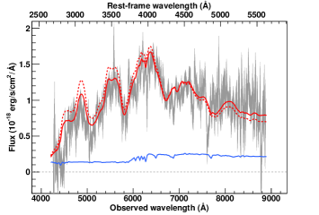
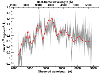
Figure 20: The SNIa 05D1dx_1013 spectrum measured at $z=0.58$ with a phase of -8.5 days. A S0(1) host model has been subtracted.

The 70 spectra of the 68 SNe Ia are presented individually in Fig. 20 - 89. In the left panel, the extracted spectrum is shown (in gray). It is not corrected for telluric features. The SALT2 best-fit model is overlayed, either with no recalibration (red dashed line) or once recalibration is applied (red solid line). The best-fit host-galaxy template is also plotted (blue solid line). The best-fit host-galaxy model, redshift and spectrum phase are noted in the figure captions. In the right panel, the host-galaxy subtracted spectrum, that is the spectrum minus the blue solid line of the left panel, is shown (in gray) with the SN model overlayed as a red solid line. The latter SN model corresponds to the full model (red solid curve) minus the host-galaxy model (blue solid curve). When the best-fit is obtained for a model with no galaxy component (the NoGalaxy cases), only the extracted spectrum (in gray) and the best-fit model without (red dashed curve) and with (red solid line) recalibration are presented.

In almost 90% of cases, the spectrum is well reproduced by SALT2. However, we find 8 spectra in our certain SN Ia sample for which the fit is not fully satisfying, at least in some wavelength regions. They mostly correspond to spectra highly contaminated by the host-galaxy signal for which the host-galaxy subtraction is difficult: SN 06D1dc ($f_{gal}$=77%), SN 06D1fx (70%), SN 06D1jz (73%), SN 06D2hu (71%), SN 07D1ad (69%) and SN 07D4dq (78%). Two spectra (SN 06D1dl and SN 07D1ab) show a sharp drop in their flux in the reddest part, hinting to a potential calibration problem beyond 9000 Å (observer frame). Moreover, in the case of SN 06D1dl, one notes quite narrow features similar to those found in SN 1991bg-like supernovae, as well as a high velocity Ca ii absorption. However, both its stretch and color are typical of a normal SN Ia. More generally, all these spectra have been unambigusouly identified as SN Ia.

Some spectra need quite a strong recalibration. This is the case for SN 07D2ct (a very distant SN Ia$\star$ at $z=0.94$), or for one spectrum of SN 06D1eb (a SN Ia at $z=0.704$). In this latter case, the phase is more than $5$ days before maximum light, and the strong recalibration could be at least partly explained by the fact that the SALT2 model is not as well constrained for early SNe Ia spectra because of the paucity of training data. In the case of SN 07D2fz, a SN Ia at $z=0.743$ that needs substantial recalibration, the SALT2 color ($c=-0.15$) is bluer than the average SNe Ia color at maximum light ($<c>^{max}=0$). The spectrum is on the contrary quite red for a SN Ia slightly before maximum. This mismatch of the spectrum and lightcurve colors explains the level of recalibration incorporated in the SALT2 fit and is at least partly due to the lack of constraining lightcurve measurements.

5.4 Catalog of non SNe Ia MOS objects

The observations with FORS1 and FORS2 allowed us to target up to 19 objects simultaneously. One of the slits was always placed on the active supernova. The other 18 were placed on a variety of targets, which included the host-galaxy galaxies of SNLS supernovae that had faded from view, variable sources, and randomly selected field galaxies. We list the redshifts of all these targets in Table LABEL:table:MOS. We use the ID column to distinguish between host-galaxy galaxies that were targeted after the transient had faded from view, live transients (using the labels SNIbc, SNII, SNII? or ?), and random field galaxies. Most redshifts are derived from two or more clearly identifiable spectral features. Redshifts based on a single feature, usually [O ii], are marked with an asterisk.

Also listed are the supernovae that were not SNe Ia. These supernovae were predominantely Type II SNe. Interestingly enough, two of these supernovae, SN 06D4eu and SN 07D2bv were subsequently identified as superluminous supernovae in Howell et al. (2013). The redshift of SN 06D4eu is derived from the host-galaxy and was measured with X-Shooter (Howell et al. 2013), whereas the redshift of SN 07D2bv was measured from the FORS spectrum.

About a sixth of the SNLS five year SN sample was observed with the MOS mode of FORS1 and FORS2, leading us to speculate that other superluminous supernovae were observed spectroscopically with Gemini and Keck during the five years of the SNLS. Indeed, Prajs et al. (2016) recently found a superluminous candidate observed at Keck.

6 Average properties of the VLT SNe Ia samples

In this section, we characterize the average properties of the SN Ia  and SN Ia$\star$ subsamples that result from the classification decribed in Sect. 5. We compare those to the properties of the same subsamples of the three year analysis (Balland et al. 2009). The new SN Ia  and SN Ia$\star$ subsamples are fully independent from those of the three year (no supernova in common and different extraction procedures) and we expect their average properties to be similar to those of their three year counterparts. Studying the properties of the new subsamples thus provides a good way to check that the conclusions drawn from the three year samples are not biased.

6.1 Spectro-photometric properties of the new VLT sample

The average photometric and spectroscopic parameters of the SN Ia and SN Ia$\star$ new subsamples are shown in Table 4. We also compute the average properties of the combined SN Ia and SN Ia$\star$ samples. For each parameter of interest, we indicate the mean value and associated error. We further indicate in parentheses the $1\sigma$ dispersion around the mean values.

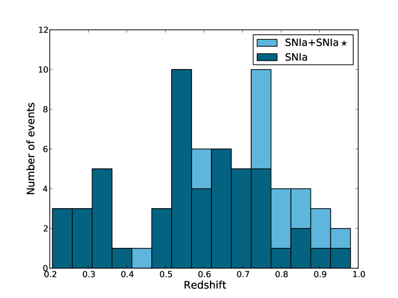
Figure 1: Redshift distribution of the VLT SNe Ia from the last two years of SNLS. SN Ia are shown in dark blue, SN Ia + SN Ia$\star$ in light blue. The mean redshift is $\langle z\rangle_{SNIa}=0.57\pm 0.03$ for the 51 SN Ia and $\langle z\rangle_{SNIa\star}=0.77\pm 0.03$ for the 16 SN Ia$\star$

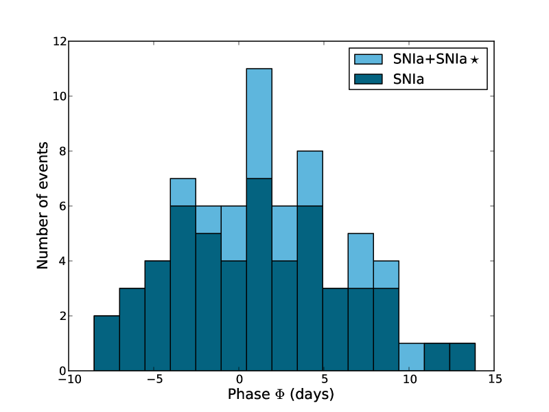
Figure 2: Phase distribution of the VLT SNe Ia from the last two years of SNLS. SN Ia are shown in dark blue, SN Ia + SN Ia$\star$ in light blue. The mean phase is $\langle\Phi\rangle_{SNIa}=1.0\pm 0.7$ days for the 51 SN Ia spectra and $\langle\Phi\rangle_{SNIa\star}=2.8\pm 0.9$ days for the 16 SN Ia$\star$ spectra

Figures 1 and 2 present the redshift, and phase distributions of the two samples. The average redshift (row 1 of Table 4 and Fig. 1) of the SN Ia$\star$ subsample ($\langle z\rangle_{SNIa\star}=0.77\pm 0.03$) is significantly higher than the one of the SN Ia  subsample ($\langle z\rangle_{SNIa}=0.57\pm 0.03$). This is expected as, given our observational strategy, spectra of distant supernovae are noisier and thus more likely to be classified as SN Ia$\star$. Indeed, as can be seen from row 4 of Table 4, SN Ia spectra have a higher $S/N$ per 5 Å bin on average ($\langle S/N\rangle_{SNIa}=5.5\pm 0.9$) than SN Ia$\star$ spectra ($\langle S/N\rangle_{SNIa\star}=1.6\pm 0.2$).

Another important parameter is the spectrum phase. As explained in Sect. 4.3, spectra observed more than 5 days past maximum are preferentially classified as a SN Ia$\star$ because confusion with SN Ib/Ic is possible (although unlikely when lightcurve information is taken into account along with the spectrum, see end of Sect. 4.3). Row 2 of Table 4 and Fig. 2 illustrate this tendency : SN Ia  spectra are marginally at a lower phase ($\langle\Phi\rangle_{SNIa}=1.0\pm 0.7$ days) than SN Ia$\star$ spectra ($\langle\Phi\rangle_{SNIa\star}=2.8\pm 0.9$ days). In particular, we note that there are no SN Ia$\star$ with phases lower than -5 days.

In the 5th row of Table 4, we give the average values of the $\gamma_{1}$ recalibration parameter. $\gamma_{1}$ is marginally higher for SN Ia$\star$ than for SN Ia ($\langle\gamma_{1}\rangle_{SNIa\star}=0.66\pm 0.39$ vs $\langle\gamma_{1}\rangle_{SNIa}=0.42\pm 0.12$).

As expected, the average host-galaxy fraction (third row of Table 4) in the best-fit model for SN Ia$\star$ spectra is higher ($\langle f_{gal}\rangle_{SNIa\star}=0.61\pm 0.04$) than for SN Ia spectra ($\langle f_{gal}\rangle_{SNIa\star}=0.39\pm 0.03$). We note that supernovae with a high host-galaxy contamination are often high redshift objects, as the reduction in the galaxy angular size of objects relative to the seeing with redshift makes it difficult to extract the supernova candidate separately from the host-galaxy.

The apparent restframe B-band magnitude $m_{B}^{*}$ is given in row 6 of Table 4. Candidates classified as SN Ia$\star$ appear, on average, fainter ($\langle m_{B}^{*}\rangle_{SNIa\star}=24.217\pm 0.086$) than SN Ia ($\langle m_{B}^{*}\rangle_{SNIa}=23.285\pm 0.127$), as they are more distant on average than the SN Ia.

We compute a distance corrected apparent magnitude as $m_{B}^{*\;c}=m_{B}^{*}-5log(d_{L}H_{0}c^{-1})$ where $d_{L}$ is the luminosity distance which depends on redshift and on cosmology through the parameter set $\{H_{0},\Omega_{M},\Omega_{\Lambda}\}$. We adopt the parameter values $\{70,0.27,0.73\}$ (Conley et al. 2011). We find a similar averaged value of $m_{B}^{*\;c}$ for the two subsamples : $\langle m_{B}^{*\;c}\rangle_{SNIa}=23.965\pm 0.045$ and $\langle m_{B}^{*\;c}\rangle_{SNIa\star}=23.981\pm 0.089$. This is somewhat surprising as we expect intrinsically fainter objects to be classified as SN Ia$\star$ rather than SN Ia, and it was indeed the case in the three year analysis. It is possible that, given the relatively small number of spectra entering the SN Ia$\star$ subsample (16 objects), and given that other competing effects (later phase or heavily host-galaxy contaminated spectra) are involved, this tendency is subdominant in our new sample.

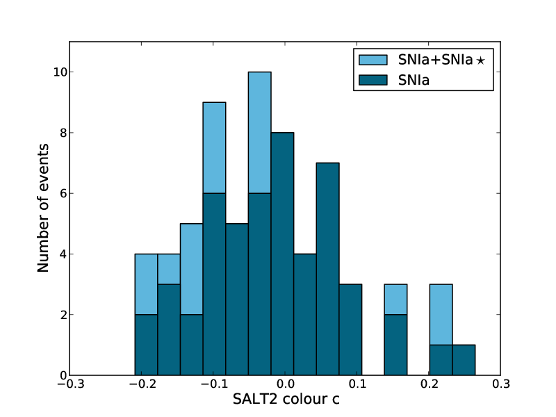
Figure 3: SALT2 color distribution of the VLT SNe Ia from the last two years of SNLS. SN Ia are shown in dark blue, SN Ia + SN Ia$\star$ in light blue. The mean color is $\langle c\rangle_{SNIa}=-0.016\pm 0.014$ for the 51 SN Ia and $\langle c\rangle_{SNIa\star}=-0.045\pm 0.033$ for the 16 SN Ia$\star$

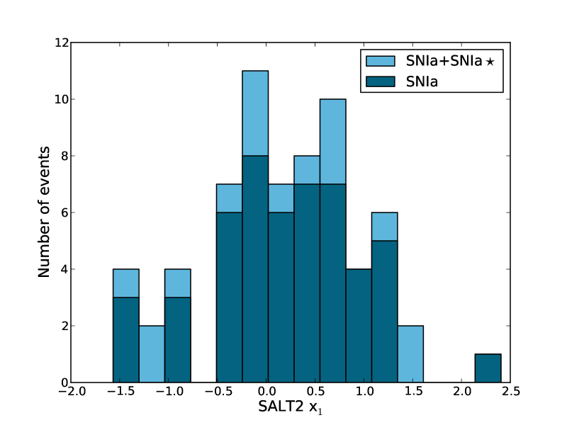
Figure 4: SALT2 $x_{1}$ distribution of the VLT SNe Ia from the last two years of SNLS. SN Ia are shown in dark blue, SN Ia + SN Ia$\star$ in light blue. The mean $x_{1}$ is $\langle x_{1}\rangle_{SNIa}=0.215\pm 0.109$ for the 51 SN Ia and $\langle x_{1}\rangle_{SNIa\star}=0.065\pm 0.226$ for the 16 SN Ia$\star$

The SALT2 color and $x_{1}$ distributions are presented in Figs. 3 and 4. Typically, a standard SN Ia/SN Ia$\star$ has its SALT2 color in the range $-0.2\leq c\leq 0.2$, and $x_{1}$ in the range -2 to 2, corresponding to a stretch factor $0.8\leq s\leq 1.2$. All our supernovae fall into these ranges, except seven: SN 06D1kg, SN 07D1bs, SN 07D2bi, and SN 07D4cy, which are redder ($c>0.2$), SN 07D4ed, which, on the contrary, is bluer ($c<-0.2$), and SN 07D1ah and SN 07D1by, which have high $x_{1}>2$ values. We discuss each of these SNe Ia in more detail.

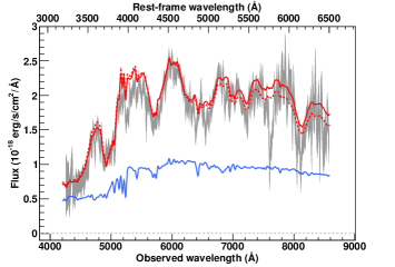
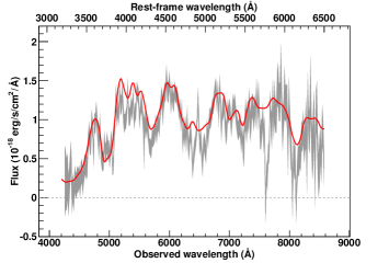
Figure 43: The SNIa 06D1kg_1477 spectrum measured at $z=0.32$ with a phase of 6.1 days. A S0(2) host model has been subtracted.

• SN 06D1kg (Fig. 43): this is a SN Ia at $z=0.32$. Its spectrum at $\sim+6$ days is presented in Fig. 43. Its color ($c=0.265$) is the largest of the sample, while its stretch is standard ($s=1.1$). The spectrum is redder than for a standard SN Ia at this phase. Explosion occured far from the center of its early-type host-galaxy and it is not clear whether its color is due to the presence of dust in the line-of-sight (no clear sign of host-galaxy Na D absorption in the spectrum). Si ii is clearly visible both around restframe 4100 Å  and 6150 Å, and S ii is also seen. There is no sign of peculiarity in the spectrum besides its reddening and it is hence classified as a SN Ia.

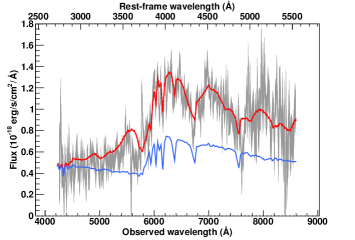
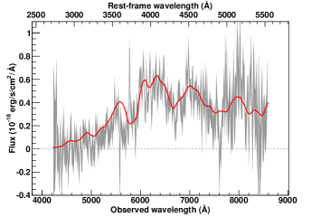
Figure 74: The SNIa 07D2bi_1514 spectrum measured at $z=0.551$ with a phase of 0.9 days. A S0(1) host model has been subtracted.

• SN 07D2bi (Fig. 74): this SN Ia  at $z=0.551$ is the second reddest object of our sample ($c=0.233$). Its lightcurve shape is standard ($s=0.99$). Its spectrum was taken slightly past maximum light and is redder than normal at this phase (with respect to color, it is more like a one-week past maximum spectrum than a spectrum at maximum light). host-galaxy Na D absorption falls off the spectral range at this redshift and no sign of the presence of dust in the line-of-sight of this supernova can be seen.

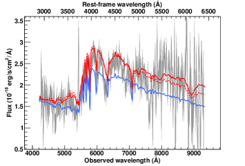
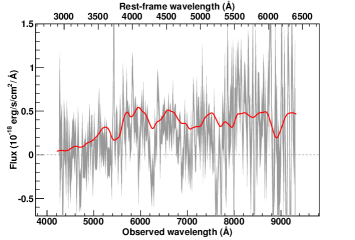
Figure 83: The SNIa$\star$ 07D4cy_1694 spectrum measured at $z=0.456$ with a phase of -0.1 days. A Sd(9) host model has been subtracted.

• SN 07D4cy (Fig. 83): as the two SNe Ia above, this SN Ia$\star$ at $z=0.456$ has a red color ($c=0.218$) and a normal stretch ($s=0.96$). The spectrum at maximum is quite noisy due to poor seeing conditions and the presence of thin cirrus. It is heavily host-galaxy contaminated, as the supernova exploded right at the center of its host-galaxy (more than 90% host-galaxy subtraction is necessary to obtain the final SN spectrum). The subtracted spectrum is unusally red for a Type Ia supernova at maximum light, but this effect could result from an imperfect host-galaxy subtraction.

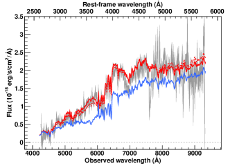
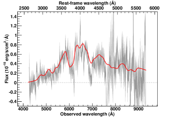
Figure 60: The SNIa$\star$ 07D1bs_1711 spectrum measured at $z=0.617$ with a phase of 0.7 days. A Sa-Sb host model has been subtracted.

• SN 07D1bs (Fig. 60): this SN Ia$\star$ at $z=0.617$ has a red color ($c=0.207$) and a normal stretch ($s=1.04$). Unlike the cases discussed above, its maximum light spectrum is quite standard and is not redder than usual at this phase. A high host-galaxy fraction has been subtracted as the supernova exploded in the vicinity of the host-galaxy center.

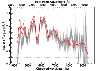
Figure 88: The SNIa 07D4ed_1731 spectrum measured at $z=0.52$ with a phase of -1.5 days. A Best fit is obtained without galactic component.

• SN 07D4ed (Fig. 88): this SN Ia  at $z=0.52$ is slightly bluer than usual ($c=-0.209$) but has a normal stretch ($s=1.01$). No host-galaxy is visible on the reference image of this supernova. The host-galaxy free -2 days spectrum shows clear Si ii $\lambda 4130$. It is bluer than standard in the restframe UV. The SALT2 model in the absence of recalibration (red dashed curve of Fig. 88) is even bluer and recalibration is necessary to fit the spectrum.

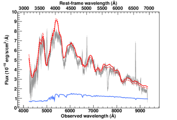
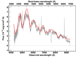
Figure 58: The SNIa-pec 07D1ah_1699 spectrum measured at $z=0.342$ with a phase of -0.6 days. A E(1) host model has been subtracted.

• SN 07D1ah (Fig. 58): the stretch and color of this SN Ia  at $z=0.342$ are $s=1.18$ and $c=-0.03$ respectively. The spectrum has an unusually weak Si ii $\lambda$ 6150 absorption for a SN Ia  at maximum light, as well as a pronounced Ca ii absorption trough. Moreover, no Si ii is seen aroung 4100 Å. It is classified as a SN Ia-pec (see Sect. 4.3).

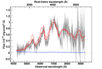
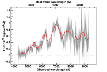
Figure 62: The SNIa 07D1by_1715 spectrum measured at $z=0.73$ with a phase of -0.5 days. A Sd(1) host model has been subtracted.

• SN 07D1by (Fig. 62): despite its slightly high stretch ($s=1.21$) and a mediocre SALT2 fit around restframe 4000 Å, SN 07D1by has a normal color $c=0.07$ and its spectrum appears normal, with a clearly visible Si ii $\lambda 4130$ absorption.

We have run the SNID package (Blondin & Tonry 2007; Blondin et al. 2011) on all the above potentially suspect spectra. The best-fits are always obtained for a normal SN Ia template, except for SN 07D1ah for which the best-fit is for the overluminous SN 1991T, confirming our identification.

The mean values of the SALT2 color and $x_{1}$ parameters are given respectively in rows 8 and 9 of Table 4. On average, we find no obvious difference in SN Ia colors ($\langle c\rangle_{SNIa}=-0.016\pm 0.014$) with respect to SN Ia$\star$ colors ($\langle c\rangle_{SNIa\star}=-0.045\pm 0.033$). The same conclusion applies for the $x_{1}$ parameter (or, equivalently, for the stretch $s$ computed in row 10 from the formula given in Guy et al. 2007) : for SN Ia, $\langle x_{1}\rangle_{SNIa}=0.215\pm 0.109$, while for SN Ia$\star$ $\langle x_{1}\rangle_{SNIa\star}=0.065\pm 0.226$ (again, quoted errors are errors on the mean), or $\langle s\rangle_{SNIa}=1.001\pm 0.010$ for SN Ia  and $\langle s\rangle_{SNIa\star}=0.988\pm 0.020$ for SN Ia$\star$.

Finally, we compute the average properties of the NoGalaxy SNe Ia (see Sect. 5.2), which we find very similar on average to those of the full sample. The dispersions of their color and stretch around the mean are also similar to those of the full sample.

We conclude from this study that the two subsamples have very similar photometric properties, on average, which suggests that the SN Ia$\star$ sample is not contaminated by non-Ia objects with respect to the SN Ia sample.

6.2 Assessing the quality of host-galaxy subtraction

As it impacts the quality of the recovered supernova spectrum and its subsequent identification, host-galaxy subtraction is a challenging step in the spectral reduction. As explained Sect. 4.3 above, we use the SALT2 model in order to separate the host-galaxy signal from the supernova. In this section we a posteriori assess the quality of the subtraction by comparing a composite host-galaxy subtracted spectrum built from supernovae with high contamination to the one made of low contamination supernovae.

We use only SN Ia spectra (excluding SN Ia$\star$) and exclude the 8 spectra discussed in Sect. 5.3. A color cut is applied ($-0.2<c<0.2$) and the phase is chosen in the range $-4<\Phi<4$ restframe days to select spectra around maximum light.

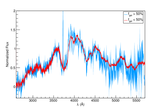
Figure 5: Comparison of the composite spectra at maximum light built from the VLT SNe Ia  of the last two years of SNLS as a function of host-galaxy contamination : $f_{gal}<50\%$ (in red) et $f_{gal}\geq 50\%$ (in blue). A $\pm 1\sigma$ range is plotted.

We split the resulting set into two subsamples, based on the value of the $f_{gal}$ parameter. These contain 17 spectra with $f_{gal}<50\%$ and 7 with $f_{gal}>50\%$, respectively. Spectra are put into the restframe and rebinned to 5 Å. The flux integral is fixed to unity in the range 4000-4500 Å (restframe). The average weighted flux and its dispersion are then computed in each wavelength bin and we obtain one average spectrum for each subsample. These two spectra are overlapped in Fig. 5. A $\pm 1\sigma$ range around each spectrum is shown.

The two spectra are very similar, showing that the host-galaxy subtraction is not grossly incorrect for the bulk of our spectra. Residual host-galaxy lines are visible as we do not attempt to subtract them (we do not model host-galaxy emission lines in the galaxy model used in SALT2, see Sect. 4.3). These are stronger in the higher contaminated sample, as expected. Absorption line residuals are also visible in the 3500 - 4500 Å region and might be due to a lack of spectral resolution in the host-galaxy model. We note that the average signal-to-noise ratio is poorer for the $f_{gal}>50\%$ spectrum, due to the small number of spectra used for this subsample and to the systematic error associated with the subtraction of the host-galaxy signal. We note a slightly depressed flux of the $f_{gal}>50\%$ spectrum with respect to the $f_{gal}<50\%$ one beyond restframe 4700 Å. This might hint toward a slight tendency to oversubtract the host-galaxy signal at higher wavelengths, but the poor $S/N$ prevents us from drawing a firm conclusion. Given that performing a clean host-galaxy subtraction is notoriously difficult, we conclude that our technique is not grossly in error.

6.3 Comparison with the VLT three year data set

In this section, we compare the average properties of the new SN Ia + SN Ia$\star$ sample with the VLT three year SN Ia + SN Ia$\star$ sample. Results are presented in Table 5. Values for the redshift, phase, host-galaxy fraction and $S/N$ ratio of the three year sample are directly taken from Balland et al. (2009), whereas the photometric parameters (B-band magnitude with or without distance correction, color, $x_{1}$ and stretch) are re-computed using the updated values of Guy et al. (2010).

From inspection of Table 5, it appears that the two VLT SN Ia + SN Ia$\star$ samples have similar photometric properties. It is also true for the spectroscopic parameters, except for the phase (row 2) and the host-galaxy fraction (row 3). The phase is indeed marginally different: the new VLT spectra have been measured $\sim 1.5$ days earlier, on average, than the VLT three year spectra. This might be due to the fact that, as experience built up along the course of the survey, SN Ia candidates were more efficiently selected in their early phase, allowing spectra to be observed closer to maximum light, on average, than during the first years of the survey. This effect was already noted in Balland et al. (2009).

The higher host-galaxy fraction of the new VLT sample can be traced back to the change in observing mode, from LSS to MOS, inducing a different extraction procedure for the two samples. For the three year sample, a photometric model of the host-galaxy was built and, whenever possible, the two components (host-galaxy and SN) were extracted at the same time. For the new sample, the host-galaxy-SN separation is performed during the identification procedure by adding a host-galaxy component to the SN model.

The fact that the two independent samples (the three year and the final two years samples) have similar spectroscopic and photometric properties shows that they are not biased (or they are biased in the same way) against the inclusion of peculiar objects or confusion with other SN types.

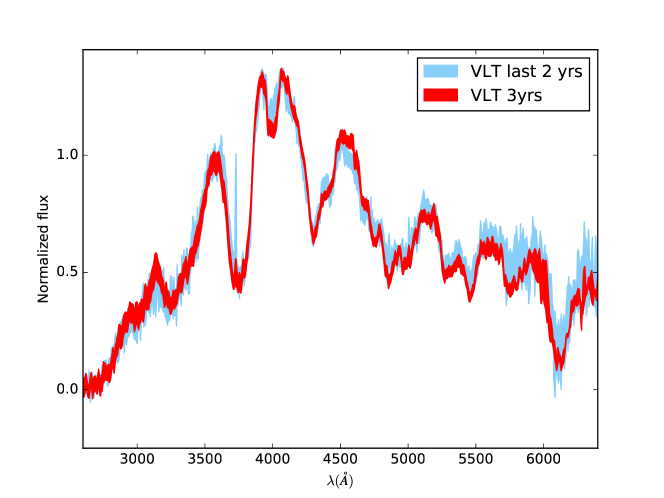
Figure 6: Comparison of the composite spectra at maximum light of the VLT three year sample (red) and the last two years of SNLS VLT sample (blue).

To illustrate this similarity, we use 47 VLT three year SN Ia spectra and 24 SN Ia spectra from our new sample around maximum light to build two average spectra using the procedure described in Sect. 6.2. The two spectra are overlapped in Fig. 6. They look remarkably similar over the studied spectral range. We note a stronger [O ii] emission in the mean spectrum of the new sample, as a consequence of not attempting to subtract host-galaxy lines in the present analysis. Some local differences are found around restframe 4000 Å and 4600 Å. The most striking difference resides in the depth of the absorption feature due to Si ii $\lambda 5970$ (blueshifted to $5750$ Å). Indeed, the VLT three year spectrum shows a deeper absorption than the spectrum of the new sample. Given the relatively small number of spectra in each subsample, such a difference could be due to the erroneous inclusion of a non SN Ia object in one of them. For example, one might argue that the inclusion of a SN 1991T like supernova in the new sample might weaken the Si ii $\lambda 5970$ absorption, but it should also alter the Ca ii region, which is not seen. Inclusion of a SN 1999aa like SN Ia  could smooth the secondary $\lambda 5970$ silicon absorption, while preserving a strong Ca ii absorption (Garavini et al. 2004), but the Si ii $\lambda 4100$ would also be affected. Besides, as discussed above, special care has been taken to eliminate peculiar events in our samples, and it is unlikely that they are polluted by such an event.

We thus confirm that the VLT three year and the new samples are consistent on average. The two samples can then be combined to build the final VLT five year spectral set, which contains 192 SNe Ia for a total of 209 spectra. This final VLT spectroscopic sample will be merged with the other SNe Ia spectra of the SNLS (from Gemini and Keck telescopes) to produce the final SNLS spectroscopic sample. The SNLS five year cosmological analysis will rely on this sample, once further photometric cuts are made (Betoule et al. 2017, in prep).

7 Properties of SNLS SNe Ia from composite spectra

In this section, we use the final VLT spectral set described above to examine how the spectra depend on color, stretch and host-galaxy mass, and to search for evolution with redshift. This analysis builds on previous works (Howell et al. 2007; Ellis et al. 2008; Foley et al. 2008a; Sullivan et al. 2009; Balland et al. 2009; Cooke et al. 2011; Foley et al. 2012; Maguire et al. 2012; Milne et al. 2015). To build composite (average) spectra, we select from the full VLT sample spectra of SNe Ia which belong to the SN Ia category (as opposed to the SN Ia$\star$ category) with phase ranging between -4 and +4 days. This ensures that the analysis benefits from the highest $S/N$ of the sample. We follow the method outline in Sect. 6.2 to build the composite spectra. Both SNe with redshift estimated from host-galaxy features and from template fitting are used. We first study the effect of color correction (Sect. 7.1), then split the sample in redshift (Sect. 7.2), stretch (Sect. 7.3) and host-galaxy mass (Sect. 7.4).

7.1 Color correction

We first divide the VLT final sample into two subsamples as a function of color. We select 40 spectra with $c<0$ and 31 with $c\geq 0$. The spectro-photometric properties of these two subsamples are shown in Table 6. The subsamples have similar properties on average, except for color and distance corrected magnitude.

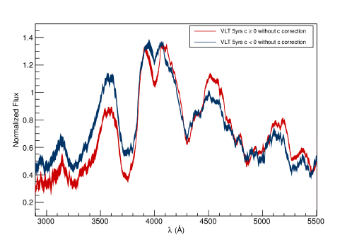
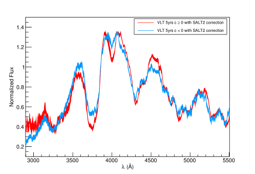
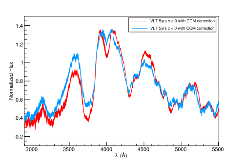
Figure 7: Comparison of composite spectra from the full VLT five year sample split in color, without color correction (top panel), with color correction using the SALT2 color law (middle panel) and with color correction using the CCM law (bottom panel). In each panel, the blue spectrum is built from $c<0$ SNe Ia, the red spectrum from $c\geq 0$ SNe Ia. No recalibration has been applied to individual spectra (see text for details). Residual host-galaxy lines have been removed. A $\pm 1\sigma$ range is plotted.

We compute a composite spectrum for each subsample before and after color correction. When a color correction is applied, either the SALT2 color law (Guy et al. 2010) or the CCM color law (Cardelli et al. 1989) are used. host-galaxy residual lines ([O ii] $\lambda\lambda 3727,3729$ and Ca ii H&K) are removed by interpolating the continuum under the lines. The SALT2 color law is derived during the training process of the SALT2 model (Guy et al. 2010). It not only captures the effects of dust extinction by the host-galaxy interstellar medium, but also at least partially the intrinsic color scatter among SNe Ia. In contrast, the CCM law is a standard dust reddening correction with the total to selective extinction parameter $R_{V}=3.1$ (Cardelli et al. 1989). After color correction using the SALT2 color law, the two average spectra are overlapping nicely over the whole spectral range (see Fig. 7), while using the CCM is less efficient, namely below $\lambda\sim 3700$ Å. This traces back to differences in the laws in this spectral region (Guy et al. 2010). Local differences already existing before correction are still present (bluer and brighter SNe Ia have weaker absorption features due to IMEs), as the color correction is required to be a smooth function of wavelength that cannot correct for finer scale differences.

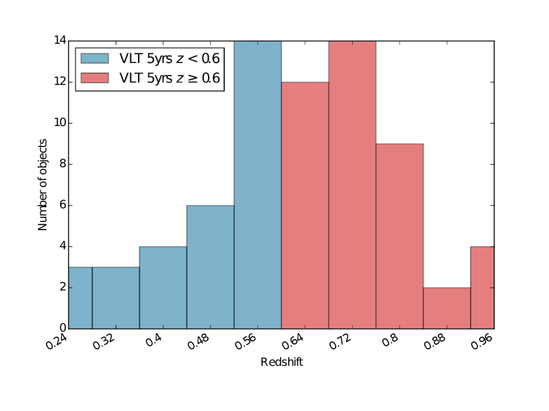
Figure 8: Redshift distribution of low ($z<0.6$, in blue) and high ($z\geq 0.6$, in red) redshift SNe Ia subsamples used to build composite spectra. The mean redshift is $\langle z\rangle_{z<0.6}=0.47\pm 0.02$ for the 30 low-$z$ SNe Ia and $\langle z\rangle_{z\geq 0.6}=0.73\pm 0.01$ for the 41 high-$z$ SNe Ia.

Similar comparisons of the effect of color laws on reddening corrections of SNe Ia spectra have been performed by various authors. Ellis et al. (2008), using a sample of 36 SNe Ia  spectra obtained at Keck within the SNLS, observe the same trend as ours (see their Fig. 8). Based on a set of HST spectra, Maguire et al. (2012) also find that the combination of the SALT2 law and SALT2 colors derived from colors of the Sifto lightcurve fitter (Conley et al. 2008) is more efficient at color correcting the spectra than the CCM color law with Sifto colors. However, the matching of the color corrected spectra is better in the latter case, while the SALT2 correction tends to overcorrect the spectra. We do not see this trend in our analysis and we choose to color correct our spectra with the SALT2 law in the following.

7.2 Redshift evolution

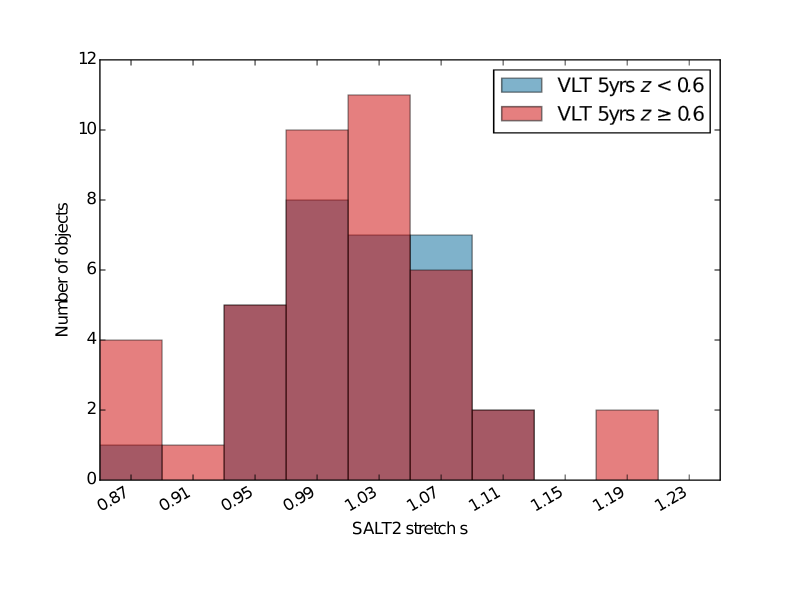
Figure 11: SALT2 stretch distribution of low ($z<0.6$, in blue) and high ($z\geq 0.6$, in red) redshift SNe Ia subsamples used to build composite spectra. The mean stretch is $\langle s\rangle_{z<0.6}=1.018\pm 0.010$ for the 30 low-$z$ SNe Ia and $\langle s\rangle_{z\geq 0.6}=1.010\pm 0.011$ for the 41 high-$z$ SNe Ia

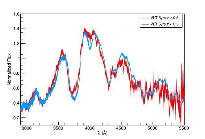
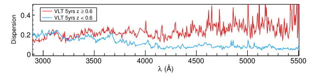
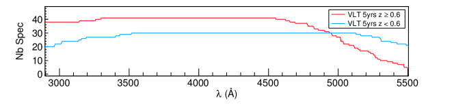
Figure 12: Top panel : Low ($z<0.6$, in blue) and high ($z\geq 0.6$, in red) redshift composite spectra around maximum light built from the VLT five year sample. A $\pm 1\sigma$ range is plotted. Individual spectra are color corrected (using SALT2 color law) and recalibrated. Residual host-galaxy lines have been removed. Middle panel : dispersion of the low (blue) and high (red) redshift composite spectra. Bottom panel : number of spectra entering the low (blue) and high (red) redshift composite spectra.

We then divide the SN Ia VLT sample into two redshift sets. We define a low redshift sample with $z<0.6$ and a high redshift with $z\geq 0.6$. They contain 30 low redshift spectra and 41 high redshift ones, respectively, with a similar phase distribution (see Table 7). The redshift, phase, color and stretch distributions of these two subamples are shown in Fig. 8 to Fig. 11. The mean spectra, built this time after applying recalibration and color correction to individual spectra, are displayed in Fig. 12. host-galaxy residual lines are removed using the technique of Sect. 7.1. In Fig. 12, the two lower panels show the dispersion of the mean spectra and the number of spectra used at each wavelength bin, respectively. They help to assess reality of observed spectral differences.

We note spectral differences between low and high redshift spectra around the Ca ii H&K and Si ii $\lambda 4130$ IME absorptions. The low redshift spectrum has deeper IME absorptions ($EW({Ca\textsc{ii}})_{z<0.6}=110\pm 3$ Å and $EW({Si\textsc{ii}})_{z<0.6}=12\pm 3$ Å) than the high redshift spectrum ($EW({Ca\textsc{ii}})_{z\geq 0.6}=102\pm 3$ Å and $EW({Si\textsc{ii}})_{z\geq 0.6}=5\pm 3$ Å).

To investigate whether these differences are significant, we select a random number of spectra in each of the two subsamples (between 15 and 30 for the low-$z$ sample and between 20 and 41 for the high-$z$ sample). We build the corresponding mean spectra and compute their flux in spectral regions where the differences are most pronounced (between 3500-3900 Å for the Ca ii H&K feature and between 3900-4100 Å for the Si ii $\lambda 4130$ feature). We repeat this process 5000 times. Using this bootstrap technique, we find that the flux is higher for the high-$z$ mean spectrum in 95.9% of cases ($2\sigma$) in the Ca ii H&K region and in 98.9% of cases ($2.5\sigma$) in the Si ii $\lambda 4130$ region. The observed increase of flux with redshift in the range [3300 - 3600] Å, due to lessened line-blanketing from iron-group elements (IGEs) with decreasing metallicity at high $z$, has been noted in all previous similar studies using independent samples (e.g., Sullivan et al. 2009; Balland et al. 2009; Maguire et al. 2012; Foley et al. 2012)

We note an increase of the dispersion for $\lambda<3800$ Å  compared to optical wavelengths for low redshift spectra (second plot of Fig. 12). This tendency is also found in Ellis et al. (2008) and Maguire et al. (2012). This SN Ia variability might be traced back to the host-galaxy properties. Indeed, this spectral zone is very sensitive to the chemical composition of the ejecta. Thanks to the SN Ia spectral synthesis models of Walker et al. (2012), Maguire et al. (2012) show that the UV dispersion is consistent with metallicity variation in the SN population. For the high redshift spectrum, the dispersion is generally larger than that of the low redshift one. No increase of the UV dispersion with respect to the one at optical wavelengths is seen in the high redshift spectrum.

7.3 Split in stretch

From table 7, it can be seen that there is no significant difference in stretch between the high and low redshift samples, given the error on the mean, whereas previous studies (e.g., Howell et al. 2007; Sullivan et al. 2009) did find a change with redshift that was consistent with a demographic evolution of SN Ia populations. This is expected as the redshift range considered in the present work is much narrower, and the average star formation rate, on which SN Ia properties depend (Sullivan et al. 2006b; Howell et al. 2007), does not change much over this range. However, it is interesting to investigate the existence of spectral differences in our sample that cannot be explained by mere selection effects. For this purpose, we split the VLT sample according to the stretch values of the SNe Ia. We use $s=1.013$, the mean stretch value of the sample, as a cut. We obtain 34 low and 37 high stretch spectra whose properties are summarized in Table 8. The two subsamples have similar properties on average, except for their mean stretch by construction.

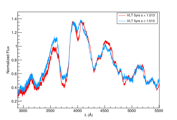
Figure 13: Comparison of composite spectra from the full VLT five year sample split in stretch. The red spectrum is for $s<1.013$ and the blue spectrum for $s\geq 1.013$. Individual spectra have been color corrected using the SALT2 color law and recalibrated. Residual host-galaxy lines have been removed.

All individual spectra are color corrected (using the SALT2 color law), recalibrated and lines from the host galaxy removed. We build composite spectra that are shown in Fig. 13. High stretch spectra are brighter in the UV below 3800 Å and have weaker absorption lines. In particular, the Ca ii H&K and Si ii $\lambda 4130$ absorption lines for the low stretch spectrum are deeper ($<EW>({Ca\textsc{ii}})_{s<1.013}=119\pm 3$ Å and $<EW>({Si\textsc{ii}})_{s<1.013}=16\pm 3$ Å) than for the high stretch spectrum ($<EW>({Ca\textsc{ii}})_{s\geq 1.013}=108\pm 3$ Å and $<EW>({Si\textsc{ii}})_{s\geq 1.013}=6\pm 3$ Å).

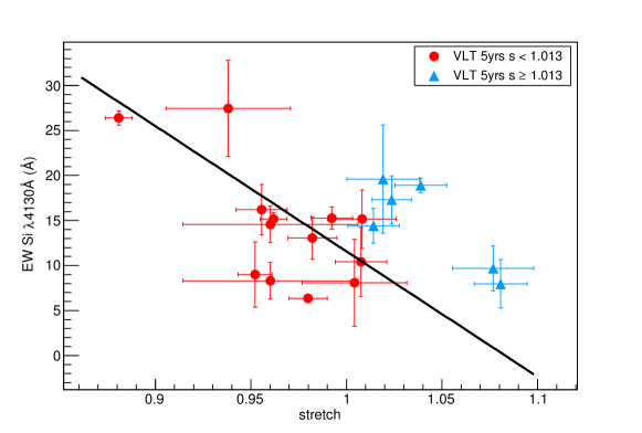
Figure 14: Correlation between EW Si ii $\lambda 4130$ and stretch measured for high S/N SNe Ia of the full VLT five year sample. The best-fit relation is $EW({Si\textsc{ii}})=(-139.3\pm 10.9)\times s+(150,9\pm 10.8)$. The low stretch ($s<1.013$) and high stretch ($s\geq 1.013$) SNe Ia are shown as red filled circles and blue triangles, respectively.

We compute the equivalent width of the Ca ii H&K and Si ii $\lambda 4130$ features, selecting now a subset of spectra with high $S/N$ for which these lines are well defined. We find a small anti-correlation between the Si ii $\lambda 4130$ equivalent width and the stretch parameter (Fig. 14):

$$EW({Si\textsc{ii}})=(-139.3\pm 10.9)\times s+(150.9\pm 10.8)\ \AA$$ (1)

In a similar analysis, Maguire et al. (2012) and Foley et al. (2012) note ejecta velocity differences as a function of stretch, high stretch SNe Ia spectra showing higher ejecta velocities on average. In particular, a blueshift is seen in Ca ii H&K, Si ii $\lambda 4130$ (Maguire et al. 2012) or in Fe ii $\lambda$3250 absorption features (Foley et al. 2012). This correlation between stretch and Ca ii H&K expansion velocity is not observed in the present analysis.

7.4 Split in host-galaxy mass

In this section, we investigate the impact of host-galaxy mass (considered as a crude proxy for metallicity or age) on our SNe Ia spectra. For each supernova in our sample, we derive its host-galaxy properties from CFHT deep reference images. Galaxy colors are fitted with a spectro-photometric code using PEGASE2 (Fioc & Rocca-Volmerange 1997, 1999) templates and trained on galaxies of the DEEP-2 survey (Davis et al. 2003, 2007). For each supernova, the host-galaxy is identified on SNLS deep reference images and is fitted to derive its type and age, yielding an estimate of the stellar mass M_stellar and specific star formation rate (sSFR). Details on this method can be found in Kronborg et al. (2010), Hardin, et al., (2017, in prep) and Roman et al. (2017). Among the 71 spectra used in Sect. 7, 62 have a reliable host-galaxy stellar mass. For the remaining 9 SNe Ia, either no host-galaxy could be associated with the SN on reference images or the spectro-photometric fit failed.

We compute the mean host-galaxy stellar mass for the two redshift subsamples of Sect. 7.2 and for the two stretch subsamples of Sect. 7.3. Differences are marginal (at the $1\sigma$ level) for the redshift subsamples ($\log{(M_{stellar})}_{z<0.6}=9.96\pm 0.14$ M_⊙ and $\log{(M_{stellar})}_{z\geq 0.6}=10.12\pm 0.11$ M_⊙) as well as for the stretch subsamples ($\log{(M_{stellar})}_{s<1.013}=10.14\pm 0.12$ M_⊙ and $\log{(M_{stellar})}_{s\geq 1.013}=9.97\pm 0.12$ M_⊙). These mass differences are not significant and are not likely to be the cause of the differences observed between low and high redshift or stretch SN Ia composite spectra.

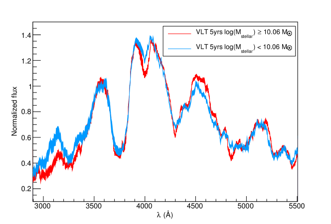
Figure 15: Comparison of composite spectra at maximum light from the full VLT five year sample host-galaxy split in stellar mass. A $\pm 1\sigma$ range is plotted. Individual spectra have been color corrected using the SALT2 color law and recalibrated. Residual host-galaxy lines have been removed.

Dividing now the SN Ia sample into two host-galaxy mass bins using the average galaxy mass of the full sample as a cut ($\log{(M_{stellar})}=10.06$ M_⊙), we end up with 27 spectra in the low mass bin and 35 in the high mass bin. These two subsamples differ in host-galaxy stellar mass (by construction) and stretch, all other parameters being equal on average (Table 9). As before, color-correction (SALT2), recalibration and removal of host-galaxy galaxy emission lines have been applied. The low and high mass composite spectra are shown in Fig. 15. Spectral differences between low and high stellar mass spectra are clearly visible in particular in the bluest part of the spectra. The low stellar mass spectrum has an excess of flux for $\lambda<3400$ Å and around the Si ii $\lambda 4130$ absorption line. Contrary to what was observed previously when spliting the sample in stretch or redshift, the two mean spectra match around the Ca ii H&K feature.

The spectral differences between low and high stellar mass average spectra might be at least partially explained by the mean stretch difference of the two subsamples ($0.031\pm 0.016$, see Table 9). Indeed, a stretch difference impacts the bluest parts of the mean spectra as seen in Sect. 7.3. Hence, the difference observed in the depth Si ii $\lambda 4130$ absorption, which is shallower in the low stellar mass spectrum ($EW({Si\textsc{ii}})_{\log{(M_{stellar})}<10.06M_{\odot}}=7\pm 1$ Å) than in its high stellar mass counterpart ($EW({Si\textsc{ii}})_{\log{(M_{stellar})}\geq 10.06M_{\odot}}=14\pm 1$ Å), might be due to stretch differences.

Selecting two new subsamples split in host-galaxy mass with the constraint that the stretch (and other spectro-photometric parameters) of the two subsamples match on average (Table 10) allows one to test the effect of the mass split alone. The resulting composite specta are shown overlapping in Fig. 16. The differences around the Si ii $\lambda 4130$ feature are significantly reduced and the equivalent widths are now similar given the error ($EW({Si\textsc{ii}})_{\log{(M_{stellar})}<10.06M_{\odot}}=8\pm 1$ Å and $EW({Si\textsc{ii}})_{\log{(M_{stellar})}\geq 10.06M_{\odot}}=9\pm 2$ Å), illustrating the impact of the stretch parameter on spectral features. However, the differences at $\lambda<3400$ Å  are still significantly present and this can be this time traced back to the difference in host-galaxy mass. A similar result has been obtained by Milne et al. (2015) using pairs of SNLS (and other survey) spectra. If confirmed, this UV flux difference might be used as a third SNe Ia standardization parameter beyond stretch and color (see Sect. 8.3 for discussion).

8 Discussion

8.1 Origin of the spectral differences with redshift

From Table 7, we note that the high redshift composite spectrum of Sect. 7.2 is made of SNe Ia that are on average bluer than those entering the low redshift spectrum, with a 2.7$\sigma$ color difference ($\Delta c=-0.056\pm 0.021$). This corresponds to a 2.9$\sigma$ (distance corrected) magnitude difference of $\Delta(m_{B}^{*\;c})=0.169\pm 0.059$, the higher redshift SNe Ia being brighter than their low redshift counterparts. We note that this color difference is fully consistent with the color difference of $\Delta c=-0.05$ expected in the SNLS samples due to the spectroscopic selection of bluer and brighter SNe Ia at higher redshift (Perrett et al. 2010). As stated in Sect. 7.3, average stretch values are similar in the two samples given the error: $\Delta s=-0.008\pm 0.015$.

Using $\{\alpha\;,\;\beta\}=\{1.295\pm 0.112\;,\;3.181\pm 0.131\}$ (Guy et al. 2010), where $\alpha$ and $\beta$ are the slopes of the light curve shape - luminosity and color - luminosity relationships used to standardize SNe Ia in cosmological analyses (Astier et al. 2006), and given the above differences in stretch and color, we expect an intrinsic magnitude difference between the two SN Ia subsamples of $|\alpha\Delta s-\beta\Delta c|=0.168\pm 0.070$. This number is consistent with the magnitude difference seen in the two samples (see Table 7).

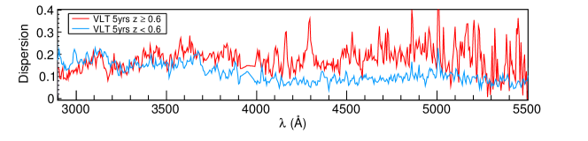
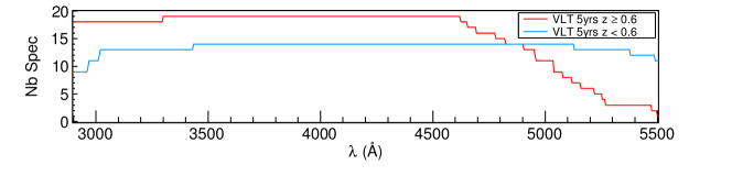
Figure 17: Same as Fig. 12 with composite spectra built from two subsamples split with matching spectro-photometric parameter distributions. Top panel : low ($z<0.6$, in blue) and high ($z\geq 0.6$, in red) redshift composite spectra. Middle panel : dispersion of the low (blue) and high (red) redshift composite spectra. Bottom panel : number of spectra entering the low (blue) and high (red) redshift composite spectra.

We now build two new subsamples at low and high redshift with the constraint that their color and stretch distributions are similar (i.e., have consistent mean and variance values). For this purpose, we identify pairs of spectra, one in each redshift bin, with matching color and stretch. We obtain 14 low and 19 high redshift spectra whose properties are shown in Table 11. The corresponding mean spectra are presented in Fig. 17. The spectral differences observed in Fig. 12 are now significantly reduced and the equivalent widths of the IMEs are consistent within error ($EW({Ca\textsc{ii}})_{z<0.6}=100\pm 4$ Å and $EW({Si\textsc{ii}})_{z<0.6}=6\pm 3$ Å  compared to $EW({Ca\textsc{ii}})_{z\geq 0.6}=105\pm 5$ Å and $EW({Si\textsc{ii}})_{z\geq 0.6}=4\pm 2$ Å).

Hence the differences previously observed tend to vanish when two populations with matching photometric properties are considered. This shows that the spectral differences observed can be attributed to a difference in the mixture of populations present in the sample at low and high redshifts, rather than to evolution with redshift. This ’demographic’ bias can be entirely attributed to the selection of bluer and brighter SNe Ia  at higher redshift in the SNLS spectroscopic sample.

Residual differences between the two composite spectra are nevertheless observed in Fig. 17. Small velocity shifts are seen in the Ca ii absorption, as well as for the two UV peaks blueward. A flux excess is also noticeable between 4500 and 5000 Å in the low redshift spectrum. Whether these differences are real or are due to residual differences in the photometric parameters of the two samples is unclear.

After selecting two subsamples with matching phase, color and stretch distributions, Maguire et al. (2012) note modest but significant differences between the low ($z\sim 0$) and high ($z\sim 0.6$) redshift average spectra. Using a bootstrap technique, they show that the low redshift spectrum has a depressed flux between 2900 and 3300 Å with respect to the high redshift one (a difference at the $3.1\sigma$ level). Using the SN Ia spectral synthesis models of Walker et al. (2012), they show that this difference could result from a metallicity evolution with redshift, the metallicity decreasing with increasing redshift. We look for comparable trends in our sample. For this purpose, we use again the bootstrap technique described in Sect. 7.2 in the same wavelength regions, this time with the two subsamples with similar photometric properties. We find that the high-redshift composite spectrum has a lower flux in the UV than the low redshift counterpart in 10.1% of cases (a significance of $1.6\sigma$). We find that the high redshift composite spectrum has a lower Ca ii H&K velocity in 13.1% of cases ($1.5\sigma$). Thus, the spectra of our sample corresponding to the same underlying supernova populations (having similar photometric parameter distributions) at low and high redshift show less significant differences than in Maguire et al. (2012), including in the UV region. This is not unexpected, as the difference in lookback times involved between our low and high redshift samples is much lower than the one in the Maguire et al. (2012) samples.

In the low and intermediate redshift samples of Maguire et al. (2012), the difference between the highest redshift of the low-$z$ sample and the lowest redshift of the high-$z$ sample is $\Delta z\sim 0.4$. This ’redshift gap’ is not present in our sample in which the redshift distribution is more uniform. In an attempt to understand the effect of such a redshift gap and check the consistency of the trends seen when splitting our sample by redshift, we re-build composite spectra, excluding successively those spectra in the range [0.55,0.65], [0.5,0.7], [0.45,0.75] and [0.4,0.8] (i.e., we impose gaps of $\Delta z$ = 0.1, 0.2, 0.3 and 0.4 centered on $z=0.6$). The differences in spectro-photometric properties between the low and high redshift subsamples are shown in Table 12 for each value of the redshift gap considered. High redshift SNe Ia are bluer (as well as brighter) with increasing gap value compared to the low redshift SNe Ia. Again, the observed differences are consistent with selecting brighter and bluer SNe Ia at higher redshift. For each gap value, we find an excess of UV flux in the high redshift spectra. Every comparison between low and high redshift spectra thus shows the same trends, independently of the subsamples used.

8.2 Stretch evolution

When our sample is split acccording to stretch value, all other parameters being equal on average, UV flux differences are observed between low stretch and high stretch composite spectra. Namely, we find a small anticorrelation between the mean stretch of the sample and the depth of the Si ii $\lambda 4130$ absorption, the latter being shallower when the stretch is higher (see Sect. 7.3). This correlation has also been noticed in Arsenijevic et al. (2008) and Walker et al. (2011). It originates as a consequence of the width-luminosity relation of SNe Ia (the so-called brigther-slower relation; Phillips 1993). More luminous SNe Ia have higher ejecta temperatures, and Si ii is partially ionized to Si iii (Nugent et al. 1995).

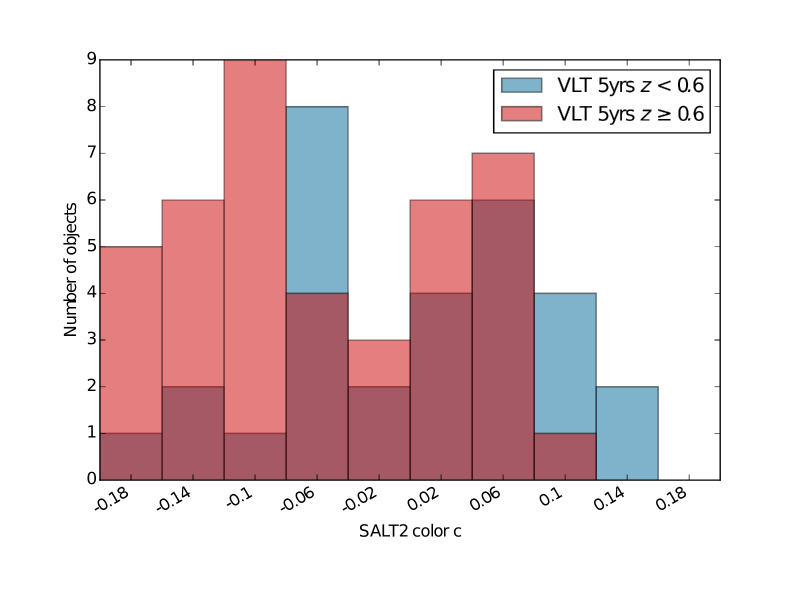
Figure 10: SALT2 color distribution of low ($z<0.6$, in blue) and high ($z\geq 0.6$, in red) redshift SNe Ia subsamples used to build composite spectra. The mean color is $\langle c\rangle_{z<0.6}=0.001\pm 0.015$ for the 30 low-$z$ SNe Ia and $\langle c\rangle_{z\geq 0.6}=-0.055\pm 0.014$ for the 41 high-$z$ SNe Ia.

The kinetic energy of the explosion is higher for higher ⁵⁶Ni mass and a correlation between the expansion scale and stretch is expected (see, e.g., Howell et al. 2006). As explained earlier, Maguire et al. (2012) do observe such a correlation: the Ca ii H&K velocity increases with stretch (see their Figs. 7 and 10) producing a spectral difference at the $3.4\sigma$ level in the calcium region. However, neither the present work nor Foley et al. (2012) find evidence for this effect. As noted by Maguire et al. (2012), the absence of spectra with $s>1.05$ in the Foley et al. (2012) sample might be responsible for this, the higher stretch spectra contributing the most to a shift in the ejecta velocity. When the 17 HST spectra with $s>1.05$ are excluded from the Maguire et al. (2012) sample, the difference between the composite spectra at low and high stretch in the Ca ii region is considerably reduced and becomes statistically insignificant (less than $1\sigma$ significance). The observation of a stretch-velocity correlation might thus be due to the large mean stretch difference in the original Maguire et al. (2012) samples ($\Delta<s>\sim 0.12$). This argument might explain as well why we do not see the effect in our sample: the fraction of high stretch spectra in our sample (25%) is indeed much lower than in Maguire et al. (2012)’s (41%).

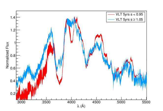
Figure 18: Comparison of composite spectra from the full VLT five year sample split by stretch while imposing a stretch gap (no spectra) between 0.95 and 1.05 in order to exacerbate the effects due to the stretch. Individual spectra have been color corrected using the SALT2 color law and recalibrated. Residual host-galaxy lines have been removed.

To test this hypothesis, we create two new subsamples by excluding all spectra with stretches in the range $0.95<s<1.05$ yielding a mean stretch difference comparable to the one of Maguire et al. (2012). Figure 18 shows an overlap of the two composite spectra computed from our new samples. The difference in the IME absorption regions are stronger than before, illustrating the impact of the mean stretch on the composite spectra; however, no significant differences beyond the ones seen in Fig. 13 (see Sect. 7.3) are observed in the velocities of IME ejecta. This leaves us either with the possibility that the mean stretch difference between our samples is not large enough or that the effect is blurred by the IME peculiar velocities in spectra for which the redshift has been estimated from SN features. Indeed, in the construction of the mean spectra, we use both SNe Ia whose redshift has been estimated from host-galaxy lines and from our spectral template fitting. If there are subtle velocity effects in the spectra, they may be washed out by using the template fitting. As about 25% of redshifts have been obtained from this technique in the present sample, as opposed to 6% in Maguire et al. (2012), this might be a non negligible effect and a limitation to the present comparison.

A possible explanation of the spectral differences observed as a function of stretch could be the existence of two (or more) distinct SN Ia  populations, with distinct stretch and spectral properties. Based on the A+B model (Scannapieco & Bildsten 2005), Howell et al. (2007) identify in a sample of SNe Ia obtained from various sources in the range $0.1<z<0.75$ a delayed and a prompt component, with a mean stretch of $s\sim 0.95$ and $s\sim 1.08$, respectively. The mean stretch of our two subsamples are indeed very similar to those values ($\sim 0.96$ and $s\sim 1.06$, see Table 8) and it is tempting to invoke the existence of these two populations in our samples.

However, if such two populations coexist at different redshifts in proportions predicted by the A+B model (in agreement with the ratios of prompt to delayed SNe Ia observed in SNfactory (Aldering et al. 2002) data by Childress et al. 2013), one would expect a stretch increase of the whole SN Ia  population of about 8% from $z=0$ to $1.1$ (Howell et al. 2007). Assuming the increase is linear in cosmic time and provided that our sample selection reflects the global properties of the underlying SN Ia population, one expects a $\sim 2$% increase in the stretch of the spectra used to create composites ($z=0.47$ to $0.73$). We find instead a moderate decrease of the mean stretch of $\lesssim 1$% from $z=0.47$ to $0.73$. This tends to show that the differences observed in our sample trace back to the selection effects of the survey, rather than to a demographic shift in the SN Ia populations with redshift.

8.3 Spectral differences with host-galaxy properties

SNe Ia photometric properties correlate with their environment (e.g., Sullivan et al. 2006b; Rigault et al. 2013; Childress et al. 2013). Brighter supernovae with higher stretch explode preferentially in late-type star-forming spiral galaxies (e.g., Hamuy et al. 1995, 2000; Sullivan et al. 2006b; Howell et al. 2007). Moreover, once corrected for stretch and color, SNe Ia are 10% brighter on average in massive later type galaxies, which also tend to have higher metalicity (e.g. Sullivan et al. 2010; Lampeitl et al. 2010; Kelly et al. 2010). From Table 10, we see that SNe Ia are marginally brighter in high mass host-galaxy galaxies by 0.1 mag, in agreement with this trend.

In terms of spectral shape, we find that the high stretch and low host-galaxy stellar mass SNe Ia have weaker Si ii $\lambda 4130$ absorptions (Sect. 7.3), in agreement, for example, with Bronder et al. (2008) who showed that SNe Ia in spiral galaxies have weaker IME absorptions than those in elliptical galaxies. We also find that SNe Ia with high stellar mass host-galaxies (all other parameters matching on average) have a significantly lower flux in the 3000-3500 Å UV region of their spectra. Interestingly, this is the region where Ellis et al. (2008) and Maguire et al. (2012) observe an increased dispersion in their spectral samples, whether split in stretch or redshift. Part of this effect could be explained by the diversity of host-galaxy properties of the SNe Ia entering the composite spectra in these studies. However, while some theoretical studies have shown that UV spectra are indeed affected by host-galaxy metallicity in a way that causes an increase in SN Ia variability in this region of the spectrum (e.g., Hoeflich et al. 1998; Lentz et al. 2000; Sauer et al. 2008), it cannot be to such an extent as to account for the full increase in dispersion observed, as noticed by Ellis et al. (2008) and Maguire et al. (2012). Nevertheless, the analysis of the present VLT spectral set supports the importance of host-galaxy parameters in understanding SNe Ia properties.

Recently, Roman et al. (2017) have estimated the host-galaxy restframe $U-V$ color at the location of the supernova explosion, using a sample of 882 SNe Ia host-galaxies from the SNLS, the SDSS and local surveys. They show that there is a significant difference between this local color and the global restframe $U-V$ color, the latter being bluer at all redshifts. Moreover, performing a cosmological fit to the SNe Ia JLA data (Betoule et al. 2014), they find the Hubble residuals to be more correlated with local color than with the host-galaxy stellar mass or global color and conclude that local color conveys more physical information on the lightcurve properties than the host-galaxy stellar mass. Using the local color as a third lightcurve standardization variable reduces the total dispersion in the Hubble diagram by $\sim 7$ % relative to using only stretch and color for standardization.

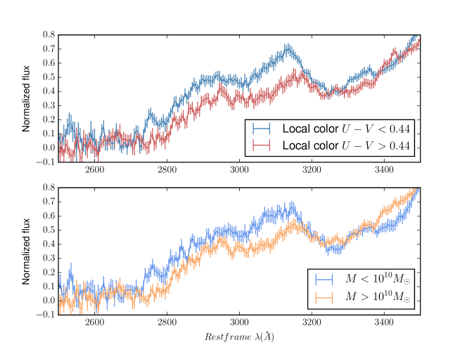
Figure 19: Comparision of composite spectra obtained when spliting the sample according to local color (top panel) or mass (bottom panel). The cut are made at the sample average value.

The Roman et al. (2017) analysis involves 397 SNLS SNe Ia host galaxies. For a fraction of these, the supernova spectrum has been observed at the VLT and belongs to the sample presented in this paper. We use these spectra along with the measurement of the corresponding host-galaxy restframe $U-V$ local color provided by Roman et al. (2017) to compute two composite spectra in two bins of local color. As before, the split value is the sample average of the relevant variable (here $<U-V>_{local}=0.439$) and only spectra with phases in the range $-4<\phi<+4$ days are considered. Spectra are color corrected and recalibrated individually. In Fig. 19, we show the two spectra in the 2500-3500 Å region (top panel). For comparison, we also show the spectra obtained in the same spectral region when splitting our sample according to the host-galaxy mass (bottom panel, see 7.4). The difference obtained with a cut in local $U-V$ is slightly more pronounced than the one with a cut in host-galaxy mass. Chosing the sample median $U-V$ rather than the average value has basically no impact on the difference seen. Moreover, excluding from the composites those spectra for which the redshift has been obtained from the SN features rather than from host-galaxy lines does not modify the result. This analysis supports the existence of a variation in the UV spectral properties of the SNe Ia populations linked to their environment. As shown in Roman et al. (2017), this link can be exploited to further standardize SNe Ia properties and reduce Hubble residuals.

9 Conclusion

The SNLS experiment benefited from exceptional spectroscopic surveys, with a total of $\sim 1500$ hours of observation on 8-10m class telescopes, including the VLT with two ESO large programs. Special attention was paid to assessing the type and determining the redshift of the SN Ia candidates using a combination of SALT2 and visual inspection.

In the present paper, we publish for the first time the spectra of the SNe Ia measured at the VLT during the last two years of SNLS. 51 SNe Ia  were identified as SN Ia (certain SNe Ia), 16 as SN Ia$\star$  (probable SNe Ia) and one object was found to be peculiar (SN 1991T like). These SNe Ia and SNe Ia$\star$ subsamples have on average very similar photometric and spectroscopic properties (color, stretch and $B$-band absolute magnitude at maximum light), which suggests that the SNe Ia$\star$ sample is not contaminated by non-Ia-objects. The host-galaxy subtraction is well under control, spectra with low and high host-galaxy contamination being remarkably similar.

This new VLT sample completes the VLT three year spectral data set which contains spectra of identified SNe Ia measured in LSS mode at the VLT during the first three years of operation of the survey (Balland et al. 2009). We find that the two VLT samples have similar spectro-photometric properties and spectra on average. Once combined to build the final VLT spectroscopic sample of SNLS, there are 192 SNe Ia for a total of 209 spectra. When Gemini and Keck spectra are added to the VLT spectral set, the final SNLS spectroscopic sample contains 427 identified SNe Ia and SNe Ia$\star$. This is the largest intermediate to high redshift SN Ia sample to date and the final SNLS cosmology analysis will rely on it (Betoule et al. 2017, in prep).

With this exceptional sample in hand, we have studied SNe Ia spectral and photometric properties at intermediate to high redshift. We have reassesed the key question of a possible evolution of SNe Ia properties with redshift in the light of this new sample. Using color corrected VLT spectra around maximum light ($-4<\Phi<4$ days), we find that:

1. the spectral comparison between low and high redshift SNe Ia shows an increase of their UV flux with redshift. Brighter and bluer SNe Ia are observed at higher redshift, in full quantitative agreement with what one expects from the spectroscopic selection process of SNLS (Perrett et al. 2010). No definite sign of intrinsic evolution of the SNe Ia properties with redshift is seen in the present sample.

2. SNe Ia in more massive galaxies have a higher stretch on average. Once this stretch difference is accounted for, a residual flux excess is found in the [3000-3400] Å region for SNe Ia with low mass host-galaxies. The same trend is observed for SNe Ia with low local $U-V$ color. If the SNe Ia UV flux is indeed indexed on the host-galaxy stellar mass or local color, this could open the way toward using the latter as a third parameter beyond stretch and color in the standardization process of SNe Ia (Roman et al. 2017).

The full VLT spectral set of the SNLS experiment is remarkable for its size and homogeneity in the intermediate to high redshift window. It will be combined with the other SNLS spectroscopic samples from Gemini (Howell et al. 2005; Bronder et al. 2008; Walker et al. 2011) and Keck (Ellis et al. 2008) and used in the final SNLS cosmology analysis.

Table 1: Observing log of the VLT SNe Ia of the last two years of SNLS. The $i_{M}$ magnitude is the magnitude at observation time.

SN name	RA (J2000)	Dec (J2000)	Spectrum date (UTC)	Exp. time (s)	Seeing ($\arcsec$)	Air Mass	$i_{M}$
05D1dx	02:27:47.00	-04:01:57.1	2005-10-10	4 x 900	1.15	1.20	23.27
05D1dx	02:27:47.00	-04:01:57.1	2005-11-12	4 x 900	0.89	1.08	23.32
05D1hm	02:27:46.19	-04:43:02.0	2005-11-29	4 x 900	0.86	1.19	23.51
05D1if	02:24:29.72	-04:34:13.0	2005-12-01	4 x 900	1.12	1.11	23.50
05D2le	10:01:54.86	+02:05:34.8	2005-12-01	4 x 900	0.64	1.35	23.56
06D1bg	02:25:20.73	-04:06:58.2	2006-08-23	4 x 900	0.75	1.38	23.60
06D1bo	02:26:15.53	-04:20:58.6	2006-08-23	4 x 900	0.98	1.13	23.52
06D1cm	02:25:01.91	-04:28:43.2	2006-09-04	8 x 900	0.63	1.18	23.53
06D1cx	02:26:02.59	-04:14:43.7	2006-09-01	4 x 900	1.48	1.08	23.67
06D1dc	02:25:09.01	-04:33:13.2	2006-09-22	4 x 900	0.98	1.14	23.38
06D1dl	02:27:38.39	-04:32:36.6	2006-09-22	4 x 900	1.08	1.08	22.97
06D1du	02:25:40.88	-04:12:23.3	2006-09-20	3 x 750	0.76	1.07	20.80
06D1eb	02:25:03.05	-04:06:25.2	2006-09-26	6 x 900	0.74	1.08	23.45
06D1eb	02:25:03.05	-04:06:25.2	2006-10-01	3 x 750	1.06	1.07	23.38
06D1ez	02:25:41.00	-04:14:49.3	2006-10-21	3 x 750	0.89	1.07	23.44
06D1fd	02:25:54.43	-04:36:28.9	2006-10-27	3 x 750	0.65	1.27	22.37
06D1fx	02:27:41.89	-04:46:43.3	2006-11-14	4 x 900	0.99	1.07	22.75
06D1gl	02:26:53.28	-04:46:29.8	2006-11-18	9 x 900	1.06	1.08	24.06
06D1hi	02:24:30.50	-04:11:39.4	2006-11-25	4 x 900	0.93	1.08	23.24
06D1ix	02:26:33.63	-03:59:03.8	2006-12-18	4 x 900	0.68	1.44	22.85
06D1jf	02:24:17.47	-04:25:52.5	2006-12-18	4 x 900	1.39	1.11	23.41
06D1jz	02:27:11.07	-04:26:25.8	2006-12-23	4 x 900	0.79	1.25	21.73
06D1kf	02:26:49.27	-04:10:10.1	2006-12-24	4 x 900	1.10	1.07	23.37
06D1kg	02:24:32.57	-04:15:02.0	2007-01-17	3 x 750	1.25	1.29	21.91
06D1kh	02:24:50.09	-04:42:30.6	2007-01-23	6 x 900	1.66	1.32	23.74
06D2ag	10:01:43.36	+01:51:37.3	2006-01-26	3 x 750	0.70	1.12	21.97
06D2bo	10:00:52.54	+02:03:22.9	2006-02-09	6 x 900	0.64	1.13	24.15
06D2hm	09:58:44.57	+02:19:58.7	2006-12-18	4 x 900	0.64	1.16	23.16
06D2hu	09:59:56.99	+02:08:03.3	2006-12-20	4 x 900	0.84	1.30	22.16
06D2jw	09:59:37.59	+02:34:18.4	2006-12-27	6 x 900	0.82	1.26	24.13
06D4ba	22:15:35.72	-18:13:44.7	2006-07-04	4 x 900	0.77	1.16	23.58
06D4bo	22:15:28.12	-17:24:33.2	2006-07-04	4 x 900	0.71	1.03	22.73
06D4bw	22:15:03.70	-17:53:00.2	2006-07-03	6 x 900	0.74	1.05	23.41
06D4gs	22:15:14.80	-17:14:52.5	2006-09-20	3 x 750	0.84	1.28	21.59
06D4jh	22:15:31.24	-18:04:22.1	2006-11-14	4 x 900	0.59	1.09	23.02
06D4jt	22:14:45.52	-18:00:56.8	2006-11-19	4 x 900	1.13	1.39	22.96
07D1ab	02:26:44.88	-04:01:00.7	2007-01-23	4 x 900	-	1.40	22.19
07D1ad	02:27:44.72	-04:57:42.3	2007-01-24	4 x 900	1.60	1.60	21.80
07D1ah	02:27:33.33	-04:06:54.3	2007-08-27	4 x 900	1.10	1.17	24.12
07D1bl	02:27:30.62	-04:40:21.2	2007-09-04	4 x 900	1.12	1.08	25.55
07D1bs	02:26:04.32	-04:54:27.6	2007-09-08	4 x 900	1.06	1.37	23.15
07D1bu	02:27:00.37	-04:32:32.9	2007-09-08	4 x 900	1.59	1.14	22.93
07D1by	02:24:05.44	-04:32:00.6	2007-09-12	4 x 900	0.91	1.07	23.44
07D1ca	02:24:47.20	-04:50:56.0	2007-09-16	6 x 900	1.19	1.10	24.00
07D1cc	02:25:16.94	-04:06:49.7	2007-09-16	6 x 900	0.81	1.09	24.14
07D1cd	02:25:33.96	-04:45:06.5	2007-09-21	6 x 900	0.99	1.11	24.22
07D1cf	02:26:34.20	-04:58:52.3	2007-09-20	4 x 900	2.24	1.08	25.30
07D2aa	10:02:05.50	+02:25:43.4	2007-01-27	6 x 900	0.52	1.13	24.11
07D2ae	10:01:50.58	+01:52:33.6	2007-01-25	4 x 900	0.60	1.13	22.84
07D2ag	10:00:09.01	+02:09:59.2	2007-01-25	4 x 900	0.73	1.16	21.48
07D2ah	09:59:58.16	+01:53:21.9	2007-01-26	4 x 900	0.64	1.22	23.49
07D2aw	10:02:21.66	+02:27:06.6	2007-02-24	4 x 900	0.82	1.23	23.94
07D2bd	09:58:38.09	+02:07:35.4	2007-02-19	4 x 900	0.88	1.12	23.15
07D2be	10:02:08.40	+02:40:00.6	2007-02-19	4 x 900	0.90	1.20	24.03
07D2bi	09:58:46.65	+02:40:29.9	2007-02-23	4 x 900	1.00	1.13	23.58
07D2bq	10:01:51.86	+02:00:48.4	2007-02-27	4 x 900	1.33	1.13	23.10
07D2cb	10:01:27.40	+01:55:47.7	2007-03-17	4 x 900	0.96	1.12	23.24
07D2cq	10:00:47.03	+01:52:04.1	2007-03-20	4 x 900	0.94	1.26	23.34
07D2ct	10:00:17.00	+02:17:13.8	2007-03-21	6 x 900	0.82	1.35	23.88
07D2du	10:00:30.20	+01:51:30.4	2007-04-20	4 x 900	1.24	1.34	22.88
07D2fy	09:59:32.36	+02:18:00.9	2007-05-15	4 x 900	0.58	1.16	23.51
07D2fz	10:00:13.41	+02:24:16.9	2007-05-15	4 x 900	0.50	1.15	23.21
07D4aa	22:16:59.49	-17:52:03.3	2007-06-19	4 x 900	0.59	1.02	21.18
07D4cy	22:15:02.47	-17:37:43.2	2007-08-22	4 x 900	1.20	1.20	23.35
07D4dp	22:14:33.80	-17:25:58.9	2007-09-10	4 x 900	0.82	1.23	23.28
07D4dq	22:14:02.17	-17:48:43.4	2007-09-10	4 x 900	0.88	1.06	22.78
07D4dr	22:14:43.06	-17:18:34.1	2007-09-10	4 x 900	1.12	1.01	23.10
07D4ec	22:16:09.48	-18:02:18.8	2007-09-19	4 x 900	1.33	1.21	25.08
07D4ed	22:15:18.55	-18:09:52.5	2007-09-28	4 x 900	0.43	1.14	24.12
07D4ei	22:16:29.93	-17:32:05.1	2007-09-22	4 x 900	0.76	1.18	23.28

Table 1: continued.

Table 2: Spectral properties of the VLT SNe Ia of the last two years of SNLS

SN name	Type	z	z source	$\Phi$	Host model	Host fraction	$\langle S/N\rangle$
05D1dx	SNIa	$0.58\pm 0.01$	S	-8.5	S0(1)	0.21	3.2
05D1dx	SNIa	$0.58\pm 0.01$	S	12.4	S0(12)	0.63	0.9
05D1hm	SNIa	$0.587\pm 0.001$	H	4.5	E(1)	0.83	1.5
05D1if	SNIa	$0.763\pm 0.001$	H	-5.9	S0-Sa	0.54	1.0
05D2le	SNIa	$0.700\pm 0.001$	H	5.9	NoGalaxy	0	1.2
06D1bg	SNIa$\star$	$0.76\pm 0.01$	S	8.0	S0(1)	0.39	1.6
06D1bo	SNIa	$0.62\pm 0.01$	S	-3.0	Sd(1)	0.2	2.4
06D1cm	SNIa	$0.619\pm 0.001$	H	8.3	NoGalaxy	0	1.5
06D1cx	SNIa	$0.860\pm 0.001$	H	-4.2	NoGalaxy	0	1.5
06D1dc	SNIa$\star$	$0.767\pm 0.001$	H	3.8	E-S0	0.77	2.8
06D1dl	SNIa	$0.514\pm 0.001$	H	-5.2	E(1)	0.68	3.5
06D1du	SNIa	$0.24\pm 0.01$	S	-0.2	E(1)	0.04	23.3
06D1eb	SNIa	$0.704\pm 0.001$	H	-5.2	Sd(1)	0.42	4.8
06D1eb	SNIa	$0.704\pm 0.001$	H	-2.3	Sd(7)	0.49	2.6
06D1ez	SNIa	$0.692\pm 0.001$	H	7.3	S0(1)	0.31	0.8
06D1fd	SNIa	$0.350\pm 0.001$	H	4.9	Sd(13)	0.33	6.9
06D1fx	SNIa	$0.524\pm 0.001$	H	6.8	Sa-Sb	0.7	5.3
06D1gl	SNIa	$0.98\pm 0.01$	S	4.3	S0-Sa	0.31	2.3
06D1hi	SNIa$\star$	$0.803\pm 0.001$	H	-3.3	E(4)	0.75	3.8
06D1ix	SNIa	$0.65\pm 0.01$	S	3.8	Sd(1)	0.09	2.9
06D1jf	SNIa	$0.641\pm 0.001$	H	1.5	Sc(4)	0.6	1.9
06D1jz	SNIa	$0.346\pm 0.001$	H	3.3	S0(7)	0.73	23.6
06D1kf	SNIa	$0.561\pm 0.001$	H	-6.5	Sd(1)	0.26	2.3
06D1kg	SNIa	$0.32\pm 0.01$	S	6.1	S0(2)	0.5	3.7
06D1kh	SNIa$\star$	$0.882\pm 0.001$	H	7.3	E(1)	0.37	1.1
06D2ag	SNIa	$0.310\pm 0.001$	H	4.0	NoGalaxy	0	13.8
06D2bo	SNIa$\star$	$0.82\pm 0.01$	S	2.6	Sa(1)	0.54	0.6
06D2hm	SNIa	$0.56\pm 0.01$	S	7.9	Sa(3)	0.02	4.9
06D2hu	SNIa	$0.342\pm 0.001$	H	7.2	E-S0	0.71	16.1
06D2jw	SNIa$\star$	$0.90\pm 0.01$	S	-0.1	E(1)	0.47	1.7
06D4ba	SNIa	$0.70\pm 0.01$	S	9.2	Sd(2)	0.17	1.6
06D4bo	SNIa	$0.552\pm 0.001$	H	1.0	S0-Sb	0.52	5.6
06D4bw	SNIa	$0.732\pm 0.001$	H	5.8	Sa(1)	0.48	2.0
06D4gs	SNIa	$0.31\pm 0.01$	S	-4.2	E(1)	0.24	6.1
06D4jh	SNIa	$0.566\pm 0.001$	H	3.7	Sd(2)	0.49	3.3
06D4jt	SNIa$\star$	$0.76\pm 0.01$	S	2.9	Sd(1)	0.44	1.4
07D1ab	SNIa	$0.328\pm 0.001$	H	-0.2	E(1)	0.51	8.0
07D1ad	SNIa	$0.297\pm 0.001$	H	6.9	S0(12)	0.69	8.8
07D1ah	SNIa-pec	$0.342\pm 0.001$	H	-0.6	E(1)	0.26	7.6
07D1bl	SNIa	$0.636\pm 0.001$	H	2.0	E(2)	0.50	4.3
07D1bs	SNIa$\star$	$0.617\pm 0.001$	H	0.7	Sa-Sb	0.8	1.6
07D1bu	SNIa	$0.626\pm 0.001$	H	-2.8	Sd(5)	0.47	4.7
07D1by	SNIa	$0.73\pm 0.01$	S	-0.5	Sd(1)	0.05	2.6
07D1ca	SNIa$\star$	$0.835\pm 0.001$	H	1.4	Sa(1)	0.42	2.0
07D1cc	SNIa	$0.853\pm 0.001$	H	1.2	Sa-Sb	0.49	1.9
07D1cd	SNIa$\star$	$0.873\pm 0.001$	H	4.1	S0-Sa	0.88	0.6
07D1cf	SNIa	$0.500\pm 0.001$	H	-8.4	E(1)	0.33	3.1
07D2aa	SNIa	$0.899\pm 0.001$	H	-1.9	S0(12)	0.69	3.3
07D2ae	SNIa	$0.501\pm 0.001$	H	1.7	S0(1)	0.43	7.9
07D2ag	SNIa	$0.25\pm 0.01$	S	-2.6	S0(5)	0.19	19.6
07D2ah	SNIa	$0.780\pm 0.001$	H	-0.6	S0(1)	0.32	3.9
07D2aw	SNIa$\star$	$0.610\pm 0.001$	H	10.0	E(1)	0.65	1.1
07D2bd	SNIa	$0.572\pm 0.001$	H	2.1	Sa-Sb	0.66	3.5
07D2be	SNIa$\star$	$0.793\pm 0.001$	H	7.0	Sc(1)	0.54	1.3
07D2bi	SNIa	$0.551\pm 0.001$	H	0.9	S0(1)	0.64	1.6
07D2bq	SNIa	$0.535\pm 0.001$	H	-3.5	E(1)	0.6	2.0
07D2cb	SNIa	$0.694\pm 0.001$	H	1.8	Sd(1)	0.38	2.7
07D2cq	SNIa$\star$	$0.746\pm 0.001$	H	1.1	E(2)	0.62	2.6
07D2ct	SNIa$\star$	$0.94\pm 0.01$	S	1.9	Sa-Sb	0.63	0.6
07D2du	SNIa	$0.538\pm 0.001$	H	-1.4	E(1)	0.39	3.3
07D2fy	SNIa	$0.72\pm 0.01$	S	0.3	NoGalaxy	0	2.4
07D2fz	SNIa	$0.743\pm 0.001$	H	-1.4	E-S0(1.0)	0.18	4.7
07D4aa	SNIa	$0.207\pm 0.001$	H	13.9	Sb-Sc	0.28	32.9
07D4cy	SNIa$\star$	$0.456\pm 0.001$	H	-0.1	Sd(9)	0.9	0.6
07D4dp	SNIa$\star$	$0.743\pm 0.001$	H	-1.8	Sd(11)	0.7	2.7
07D4dq	SNIa	$0.554\pm 0.001$	H	1.9	E(3)	0.78	5.7
07D4dr	SNIa	$0.772\pm 0.001$	H	2.2	E(4)	0.69	2.7
07D4ec	SNIa	$0.653\pm 0.001$	H	-4.0	Sa-Sb	0.76	2.0
07D4ed	SNIa	$0.52\pm 0.01$	S	-1.5	NoGalaxy	0	3.0
07D4ei	SNIa	$0.37\pm 0.01$	S	-6.7	S0(1)	0.39	1.5

Table 2: continued.

Table 3: Catalog of redshifts and identifications of the non-SN Ia objects measured in MOS mode at the VLT during the SNLS survey. We use the ID column to distinguish between host galaxies that were targeted after the transient had faded from view, live transients (using the labels SNIbc, SNII, SNII? or ?), and random field galaxies. An asterisk next to a redshift value denotes a redshift obtained from a single identified line.

Name	RA (J2000)	Dec (J2000)	z	ID
	02:25:51.01	-04:38:38.6	0.996*	Field Galaxy
05D1hb	02:24:28.93	-04:45:23.7	0.764	?
	22:16:44.39	-17:20:18.8	0.784	Field Galaxy
05D4jy	22:16:23.06	-17:47:01.6	0.869	?
06D1aq	02:26:57.80	-04:03:43.6	0.332	?
	02:26:15.82	-04:20:49.9	0.178	Field Galaxy
	02:25:09.01	-04:33:13.2	0.269*	Field Galaxy
	02:25:09.01	-04:33:13.2	0.767	Field Galaxy
06D1dv	02:26:36.85	-04:44:37.5	0.062	SNIbc
	02:26:36.70	-04:44:33.7	0.700	Field Galaxy
06D1hc	02:24:48.25	-04:56:03.6	0.555*	SNII?
06D1jd	02:27:36.19	-04:31:56.6	0.324	SNII
06D1jx	02:24:34.75	-04:57:51.7	0.14	SNII
	10:01:43.28	+01:51:35.1	0.309	Field Galaxy
	10:01:43.67	+01:51:37.3	0.794*	Field Galaxy
	10:01:43.74	+01:51:38.7	0.682*	Field Galaxy
06D2bb	09:59:35.02	+02:17:10.1	0.313	SNII?
06D2bt	09:59:01.76	+02:36:59.1	0.079	SNII
	09:59:57.22	+02:07:57.2	0.658*	Field Galaxy
06D2iy	10:01:35.56	+02:26:46.8	0.392	SNII?
06D4eu	22:15:54.29	-18:10:45.6	1.588	SLSN
07D1bw	02:27:57.03	-04:37:27.6	0.286	SNII?
07D1cd	02:25:33.96	-04:45:06.5	0.873	?
07D1ci	02:25:36.71	-04:43:26.0	0.319	SNII?
	02:25:36.54	-04:43:26.9	0.319	Field Galaxy
07D2ab	10:02:25.74	+02:19:39.8	0.312	SNII
07D2an	10:00:08.93	+02:36:14.1	0.135	SNII
07D2at	10:02:15.70	+02:05:26.1	0.216	SNII?
07D2bv	10:00:06.63	+02:38:35.8	1.50	SLSN
07D2ca	09:58:49.62	+02:31:17.3	0.507	SNII?
07D2ge	10:01:28.26	+02:42:31.9	0.084	SNII
07D4af	22:16:23.34	-18:12:35.8	0.135	SNII
07D4ck	22:16:02.21	-17:39:42.4	0.581	SNII?
	22:14:33.72	-17:25:57.7	0.743	Field Galaxy
07D4ds	22:15:54.73	-17:44:54.8	0.338	?
07D4dt	22:13:50.13	-17:36:51.8	0.677	?
07D4ee	22:15:29.69	-18:04:40.1	0.470	?
03D1ad	02:27:32.66	-04:29:23.7	0.524	Host galaxy
	02:27:32.66	-04:29:25.2	0.525	Field Galaxy
03D1af	02:24:12.67	-04:26:14.2	0.603	Host galaxy
03D1am	02:24:13.84	-04:26:02.0	0.556	Host galaxy
	02:24:13.97	-04:25:53.1	0.958*	Field Galaxy
03D1ap	02:26:35.46	-04:46:03.8	0.513	Host galaxy
03D1aq	02:25:03.08	-04:05:01.8	0.706	Host galaxy
03D1aw	02:24:14.72	-04:31:01.4	0.582	Host galaxy
03D1bc	02:27:38.48	-04:41:48.5	0.383	Host galaxy
	02:27:37.97	-04:41:59.0	0.384	Field Galaxy
03D1bg	02:27:05.91	-04:47:34.4	0.512	Host galaxy
03D1by	02:27:54.03	-04:03:04.2	0.378	Host galaxy
03D1ch	02:24:29.12	-04:09:54.9	0.265	Host galaxy
03D1da	02:25:03.19	-04:05:39.3	0.785	Host galaxy, AGN
	02:25:04.47	-04:05:34.4	0.172	Field Galaxy
03D1dg	02:25:19.84	-04:30:46.0	0.496	Host galaxy
03D1ea	02:27:50.37	-04:05:01.9	0.312	Host galaxy
03D1et	02:24:26.93	-04:47:54.4	0.855	Host galaxy
03D1ft	02:27:07.44	-04:04:38.7	0.491	Host galaxy
03D1fy	02:27:16.05	-04:24:33.4	0.177	Host galaxy
03D1gi	02:25:18.13	-04:31:55.5	0.525*	Host galaxy
03D1gl	02:27:27.82	-04:08:07.0	0.634	Host galaxy, AGN
03D4au	22:16:09.92	-18:04:39.0	0.468	Host galaxy
03D4az	22:15:47.78	-18:07:51.2	0.409*	Host galaxy
03D4cb	22:15:41.48	-18:12:44.8	0.517	Host galaxy
03D4cl	22:15:38.20	-18:06:26.8	0.90*	Host galaxy, AGN
03D4dl	22:13:35.29	-17:18:03.2	0.305	Host galaxy
03D4ec	22:14:43.72	-17:21:40.7	1.016*	Host galaxy
03D4ed	22:16:19.76	-17:31:27.5	0.860*	Host galaxy
03D4ev	22:16:51.40	-17:20:03.1	0.538	Host galaxy
03D4fb	22:14:27.22	-17:22:40.2	0.291	Host galaxy
03D4gj	22:16:01.40	-18:05:20.7	0.318	Host galaxy
04D1aa	02:26:06.22	-04:22:33.8	0.526	Host galaxy
04D1ab	02:25:37.75	-04:42:40.2	0.241	Host galaxy
	02:25:37.85	-04:42:36.0	0.265	Field Galaxy

Table 3: continued.

See online material for full table.

Table 4: Mean properties of the VLT SN Ia and SN Ia$\star$ subsamples of the last two years of SNLS. $<S/N>$ are computed in 5 Å bins. Errors are 1$\sigma$ on the mean (dispersion is given in parentheses).

	51 SNe Ia	16 SNe Ia$\star$	67 SNe Ia + SNe Ia$\star$
	53 spectra	16 spectra	69 spectra
$\langle z\rangle\;(\sigma_{z})$	$0.57\pm 0.03$ (0.18)	$0.77\pm 0.03$ (0.12)	$0.62\pm 0.02$ (0.19)
$\langle\Phi\rangle\;(\sigma_{\Phi})$	$1.0\pm 0.7$ (5.1)	$2.8\pm 0.9$ (3.7)	$1.4\pm 0.6$ (4.9)
$\langle f_{gal}\rangle\;(\sigma_{f_{gal}})$	$0.39\pm 0.03$ (0.25)	$0.61\pm 0.04$ (0.17)	$0.44\pm 0.03$ (0.25)
$\langle S/N\rangle\;(\sigma_{S/N})$	$5.5\pm 0.9$ (6.5)	$1.6\pm 0.2$ (0.9)	$4.6\pm 0.7$ (5.9)
$\langle\gamma_{1}\rangle\;(\sigma_{\gamma_{1}})$	$0.42\pm 0.12$ (0.86)	$0.66\pm 0.39$ (1.57)	$0.48\pm 0.13$ (1.06)
$\langle m_{B}^{*}\rangle\;(\sigma_{m_{B}^{*}})$	$23.285\pm 0.127$ (0.895)	$24.217\pm 0.086$ (0.342)	$23.511\pm 0.110$ (0.890)
$\langle m_{B}^{*\;c}\rangle\;(\sigma_{m_{B}^{*\;c}})$	$23.965\pm 0.045$ (0.319)	$23.981\pm 0.089$ (0.357)	$23.969\pm 0.040$ (0.326)
$\langle c\rangle\;(\sigma_{c})$	$-0.016\pm 0.014$ (0.101)	$-0.045\pm 0.033$ (0.131)	$-0.023\pm 0.013$ (0.109)
$\langle x_{1}\rangle\;(\sigma_{x_{1}})$	$0.215\pm 0.109$ (0.772)	$0.065\pm 0.226$ (0.903)	$0.180\pm 0.099$ (0.801)
$\langle s\rangle\;(\sigma_{s})$	$1.001\pm 0.010$ (0.070)	$0.988\pm 0.020$ (0.081)	$0.998\pm 0.009$ (0.072)

Table 5: Mean spectro-photometric properties of the SNLS - VLT SN Ia +SN Ia$\star$ subsamples. $<S/N>$ are computed in 5 Å bins. Errors are 1$\sigma$ on the mean (dispersion is given in parentheses). The spectra of SNe Ia identified as SN Ia_pec (two SN in the first three years sample and one in the final two years sample) have been discarded.

	VLT (first 3 years)	VLT (final 2 years)	VLT (all 5 years)
	122 SNe Ia + SNe Ia$\star$	67 SNe Ia + SNe Ia$\star$	189 SNe Ia + SNe Ia$\star$
	137 spectra	69 spectra	206 spectra
$\langle z\rangle\;(\sigma_{z})$	$0.64\pm 0.02$ (0.21)	$0.62\pm 0.02$ (0.19)	$0.63\pm 0.01$ (0.20)
$\langle\Phi\rangle\;(\sigma_{\Phi})$	$2.9\pm 0.5$ (5.6)	$1.4\pm 0.6$ (4.9)	$2.4\pm 0.4$ (5.4)
$\langle f_{gal}\rangle\;(\sigma_{f_{gal}})$	$0.24\pm 0.02$ (0.28)	$0.44\pm 0.03$ (0.25)	$0.31\pm 0.02$ (0.29)
$\langle S/N\rangle\;(\sigma_{S/N})$	$4.4\pm 0.4$ (4.6)	$4.6\pm 0.7$ (5.9)	$4.5\pm 0.4$ (5.1)
$\langle m_{B}^{*}\rangle\;(\sigma_{m_{B}^{*}})$	$23.621\pm 0.080$ (0.832)	$23.511\pm 0.110$ (0.890)	$23.582\pm 0.062$ (0.852)
$\langle m_{B}^{*\;c}\rangle\;(\sigma_{m_{B}^{*\;c}})$	$24.005\pm 0.037$ (0.407)	$23.969\pm 0.040$ (0.326)	$23.992\pm 0.028$ (0.380)
$\langle c\rangle\;(\sigma_{c})$	$-0.016\pm 0.011$ (0.121)	$-0.023\pm 0.013$ (0.109)	$-0.019\pm 0.009$ (0.117)
$\langle x_{1}\rangle\;(\sigma_{x_{1}})$	$0.390\pm 0.088$ (0.968)	$0.180\pm 0.099$ (0.801)	$0.315\pm 0.067$ (0.916)
$\langle s\rangle\;(\sigma_{s})$	$1.018\pm 0.008$ (0.087)	$0.998\pm 0.009$ (0.072)	$1.011\pm 0.006$ (0.083)

Table 6: Mean spectro-photometric properties of the blue ($c<0$) and red ($c\geq 0$) SNe Ia  samples used to build the VLT five year composite spectra. Errors are 1$\sigma$ on the mean.

	$c<0$	$c\geq 0$
Nb spec	40	31
$\langle z\rangle$	$0.66\pm 0.02$	$0.57\pm 0.03$
$\langle\Phi\rangle$	$0.3\pm 0.4$	$0.3\pm 0.4$
$\langle c\rangle$	$-0.098\pm 0.008$	$0.056\pm 0.007$
$\langle s\rangle$	$1.014\pm 0.010$	$1.013\pm 0.012$
$\langle m_{B}^{*\;c}\rangle$	$23.796\pm 0.025$	$24.091\pm 0.046$

Table 7: Mean spectro-photometric properties of the low ($z<0.6$) and high ($z\geq 0.6$) redshift SNe Ia  samples used to build the VLT five year composite spectra. Errors are 1$\sigma$ on the mean.

	$z<0.6$	$z\geq 0.6$
Nb spec	30	41
$\langle z\rangle$	$0.47\pm 0.02$	$0.73\pm 0.01$
$\langle\Phi\rangle$	$0.5\pm 0.4$	$0.1\pm 0.4$
$\langle c\rangle$	$0.001\pm 0.015$	$-0.055\pm 0.014$
$\langle s\rangle$	$1.018\pm 0.010$	$1.010\pm 0.011$
$\langle m_{B}^{*\;c}\rangle$	$24.022\pm 0.048$	$23.853\pm 0.035$

Table 8: Mean spectro-photometric properties of the low ($s<1.013$) and high ($s\geq 1.013$) stretch SNe Ia samples used to build the VLT five year composite spectra. Errors are 1$\sigma$ on the mean.

	$s<1.013$	$s\geq 1.013$
Nb spec	34	37
$\langle z\rangle$	$0.63\pm 0.03$	$0.61\pm 0.03$
$\langle\Phi\rangle$	$0.0\pm 0.4$	$0.6\pm 0.3$
$\langle c\rangle$	$-0.033\pm 0.014$	$-0.029\pm 0.016$
$\langle s\rangle$	$0.961\pm 0.007$	$1.061\pm 0.007$
$\langle m_{B}^{*\;c}\rangle$	$23.948\pm 0.040$	$23.903\pm 0.044$

Table 9: Mean spectro-photometric properties of the low ($\log{(M_{stellar})}<10.06$ M_⊙) and high ($\log{(M_{stellar})}\geq 10.06$ M_⊙) stellar mass SNe Ia samples used to build the VLT five year composite spectra. Errors are 1$\sigma$ on the mean.

	$\log{(M_{stellar})}<10.06$ M⊙	$\log{(M_{stellar})}\geq 10.06$ M⊙
Nb spec	27	35
$\langle z\rangle$	$0.58\pm 0.03$	$0.64\pm 0.03$
$\langle\Phi\rangle$	$0.2\pm 0.4$	$0.3\pm 0.4$
$\langle c\rangle$	$-0.035\pm 0.018$	$-0.030\pm 0.014$
$\langle s\rangle$	$1.027\pm 0.011$	$0.996\pm 0.012$
$\langle m_{B}^{*\;c}\rangle$	$23.940\pm 0.057$	$23.922\pm 0.039$
$\langle\log{M_{stellar}}\rangle$	$9.31\pm 0.10$ M⊙	$10.64\pm 0.06$ M⊙

Table 10: Mean spectro-photometric properties of the low ($\log{(M_{stellar})}<10.06$ M_⊙) and high ($\log{(M_{stellar})}\geq 10.06$ M_⊙) stellar mass SNe Ia samples with matching photometric parameter distributions. Errors are $1\sigma$ on the mean.

	$\log{(M_{stellar})}<10.06$ M⊙	$\log{(M_{stellar})}\geq 10.06$ M⊙
Nb spec	18	18
$\langle z\rangle$	$0.59\pm 0.03$	$0.65\pm 0.03$
$\langle\Phi\rangle$	$-0.1\pm 0.6$	$0.6\pm 0.6$
$\langle c\rangle$	$-0.038\pm 0.023$	$-0.036\pm 0.023$
$\langle s\rangle$	$1.014\pm 0.013$	$1.014\pm 0.013$
$\langle m_{B}^{*\;c}\rangle$	$23.994\pm 0.072$	$23.904\pm 0.054$
$\langle\log{M_{stellar}}\rangle$	$9.35\pm 0.11$ M⊙	$10.65\pm 0.08$ M⊙

Table 11: Mean properties of the low ($z<0$) and high ($z\geq 0.6$) redshift SNe Ia samples with matching photometric parameter distribution. Errors are 1$\sigma$ on the mean.

	$z<0.6$	$z\geq 0.6$
Nb spec	14	19
$\langle z\rangle$	$0.49\pm 0.03$	$0.73\pm 0.02$
$\langle\Phi\rangle$	$0.2\pm 0.7$	$0.1\pm 0.5$
$\langle c\rangle$	$-0.073\pm 0.011$	$-0.087\pm 0.010$
$\langle s\rangle$	$1.017\pm 0.013$	$1.015\pm 0.018$
$\langle m_{B}^{*\;c}\rangle$	$23.824\pm 0.042$	$23.792\pm 0.030$

Table 12: Differences in the mean spectro-photometric properties of the low and high redshift SNe Ia  samples as a function of the redshift gap introduced between the two subsamples (see text for details). Errors are 1$\sigma$ on the mean.

z-gap	0.1	0.2	0.3	0.4
$\Delta z$	$0.26\pm 0.02$	$0.40\pm 0.04$	$0.49\pm 0.04$	$0.60\pm 0.3$
$\Delta c$	$-0.056\pm 0.021$	$-0.062\pm 0.028$	$-0.057\pm 0.033$	$-0.089\pm 0.044$
$\Delta s$	$-0.008\pm 0.015$	$0.005\pm 0.022$	$0.029\pm 0.026$	$0.019\pm 0.038$
$\Delta m_{B}^{*\;c}$	$-0.169\pm 0.059$	$-0.190\pm 0.096$	$-0.218\pm 0.093$	$-0.363\pm 0.124$

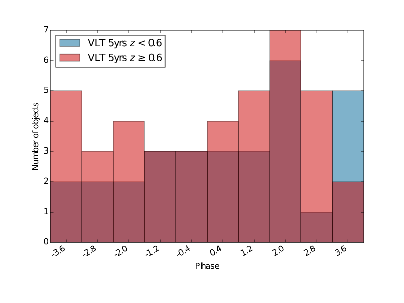
Figure 9: Phase distribution of low ($z<0.6$, in blue) and high ($z\geq 0.6$, in red) redshift SNe Ia subsamples used to build composite spectra. The mean phase is $\langle\Phi\rangle_{z<0.6}=0.5\pm 0.4$ days for the 30 low-$z$ SNe Ia and $\langle\Phi\rangle_{z\geq 0.6}=0.1\pm 0.4$ days for the 41 high-$z$ SNe Ia.

Figure 16: Same as Fig. 15, with composite spectra built from two subsamples with the constraint that the stretch and other spectro-photometric parameter distributions of the two subsamples match.

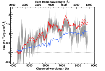
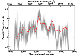
Figure 21: The SNIa 05D1dx_1046 spectrum measured at $z=0.58$ with a phase of 12.4 days. A S0(12) host model has been subtracted.

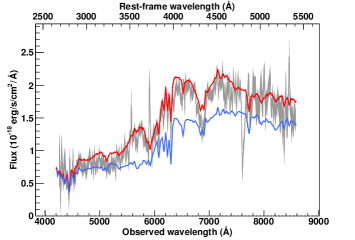
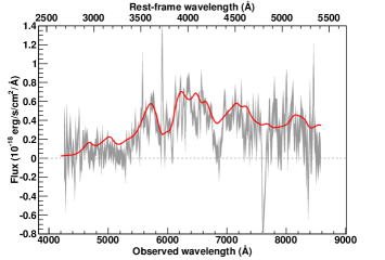
Figure 22: The SNIa 05D1hm_1063 spectrum measured at $z=0.587$ with a phase of 4.5 days. A E(1) host model has been subtracted.

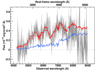
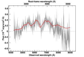
Figure 23: The SNIa 05D1if_1065 spectrum measured at $z=0.763$ with a phase of -5.9 days. A S0-Sa host model has been subtracted.

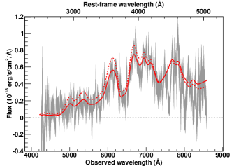
Figure 24: The SNIa 05D2le_1065 spectrum measured at $z=0.700$ with a phase of 5.9 days. Best fit is obtained without galactic component.

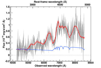
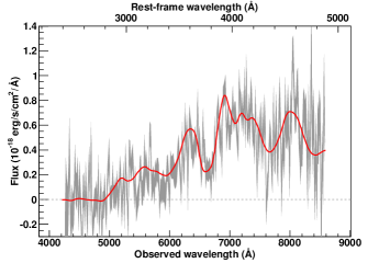
Figure 25: The SNIa$\star$ 06D1bg_1330 spectrum measured at $z=0.76$ with a phase of 8.0 days. A S0(1) host model has been subtracted.

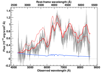
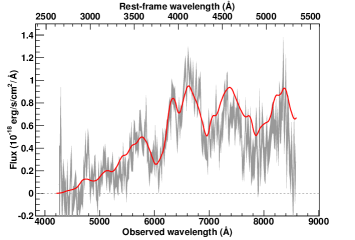
Figure 26: The SNIa 06D1bo_1330 spectrum measured at $z=0.62$ with a phase of -3.0 days. A Sd(1) host model has been subtracted.

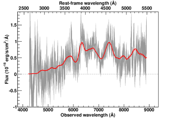
Figure 27: The SNIa 06D1cm_1342 spectrum measured at $z=0.619$ with a phase of 8.3 days. Best fit is obtained without galactic component.

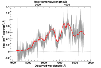
Figure 28: The SNIa 06D1cx_1339 spectrum measured at $z=0.860$ with a phase of -4.2 days. Best fit is obtained without galactic component.

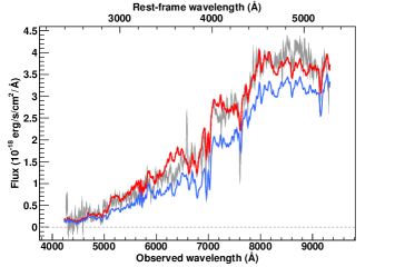
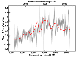
Figure 29: The SNIa$\star$ 06D1dc_1360 spectrum measured at $z=0.767$ with a phase of 3.8 days. A E-S0 host model has been subtracted.

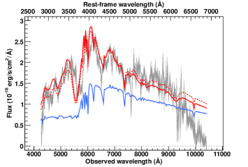
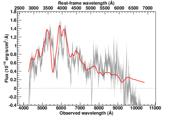
Figure 30: The SNIa 06D1dl_1360 spectrum measured at $z=0.514$ with a phase of -5.2 days. A E(1) host model has been subtracted.

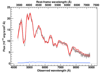
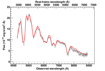
Figure 31: The SNIa 06D1du_1358 spectrum measured at $z=0.24$ with a phase of -0.2 days. A E(1) host model has been subtracted.

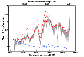
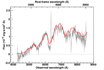
Figure 32: The SNIa 06D1eb_1364 spectrum measured at $z=0.704$ with a phase of -5.2 days. A Sd(1) host model has been subtracted.

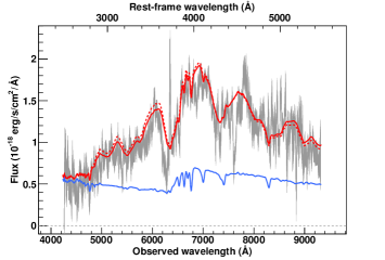
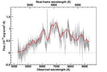
Figure 33: The SNIa 06D1eb_1369 spectrum measured at $z=0.704$ with a phase of -2.3 days. A Sd7 host model has been subtracted.

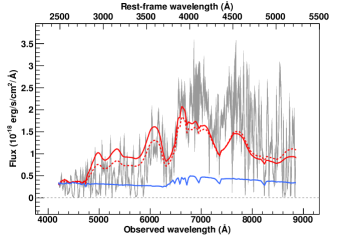
Figure 34: The SNIa 06D1ez_1389 spectrum measured at $z=0.692$ with a phase of 7.6 days. A S01 host model has been subtracted.

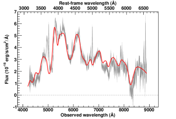
Figure 35: The SNIa 06D1fd_1395 spectrum measured at $z=0.350$ with a phase of 4.9 days. A Sd(13) host model has been subtracted.

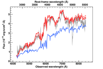
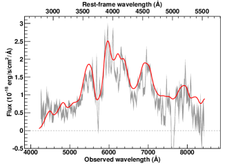
Figure 36: The SNIa 06D1fx_1413 spectrum measured at $z=0.524$ with a phase of 6.8 days. A Sa-Sb host model has been subtracted.

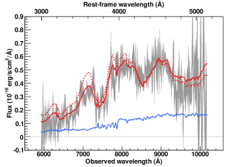
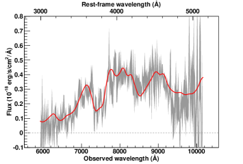
Figure 37: The SNIa 06D1gl_1417 spectrum measured at $z=0.98$ with a phase of 4.3 days. A S0-Sa host model has been subtracted.

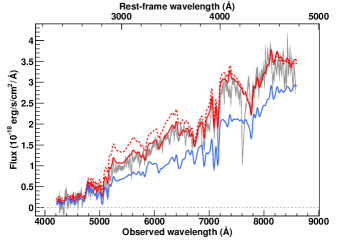
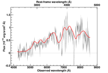
Figure 38: The SNIa$\star$ 06D1hi_1424 spectrum measured at $z=0.803$ with a phase of -3.3 days. A E(4) host model has been subtracted.

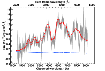
Figure 39: The SNIa 06D1ix_1447 spectrum measured at $z=0.65$ with a phase of 3.8 days. A Sd(1) host model has been subtracted.

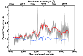
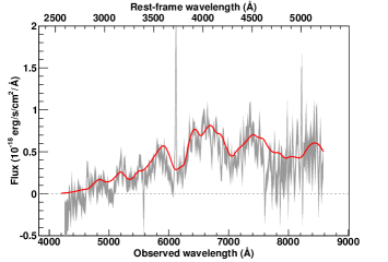
Figure 40: The SNIa 06D1jf_1447 spectrum measured at $z=0.641$ with a phase of 1.5 days. A Sc(4) host model has been subtracted.

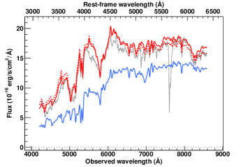
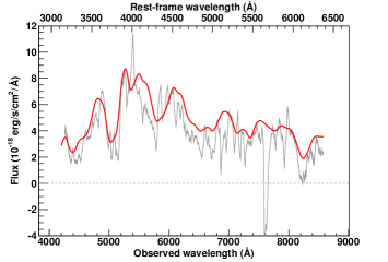
Figure 41: The SNIa 06D1jz_1452 spectrum measured at $z=0.346$ with a phase of 3.3 days. A S0(7) host model has been subtracted.

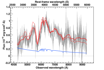
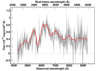
Figure 42: The SNIa 06D1kf_1453 spectrum measured at $z=0.561$ with a phase of -6.5 days. A Sd(1) host model has been subtracted.

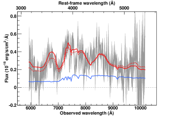
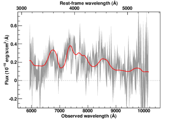
Figure 44: The SNIa$\star$ 06D1kh_1483 spectrum measured at $z=0.882$ with a phase of 7.3 days. A E(1) host model has been subtracted.

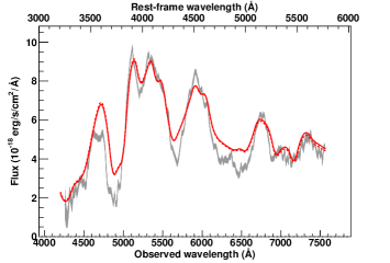
Figure 45: The SNIa 06D2ag_1121 spectrum measured at $z=0.310$ with a phase of 4.0 days. A Best fit is obtained without galactic component.

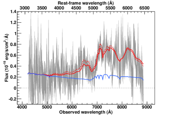
Figure 46: The SNIa$\star$ 06D2bo_1134 spectrum measured at $z=0.82$ with a phase of 2.6 days. A Sa(1) host model has been subtracted.

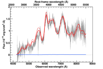
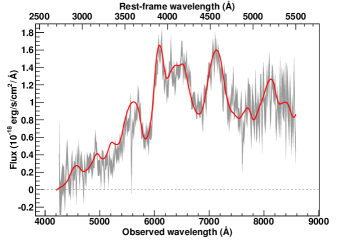
Figure 47: The SNIa 06D2hm_1447 spectrum measured at $z=0.56$ with a phase of 7.9 days. A Sa(3) host model has been subtracted.

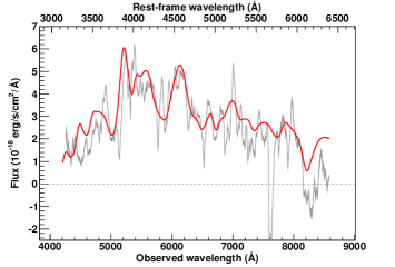
Figure 48: The SNIa 06D2hu_1449 spectrum measured at $z=0.342$ with a phase of 7.2 days. A E-S0 host model has been subtracted.

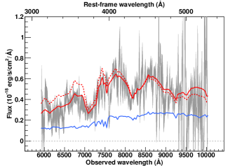
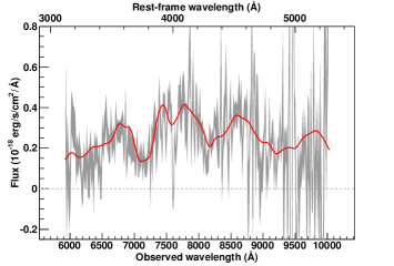
Figure 49: The SNIa$\star$ 06D2jw_1456 spectrum measured at $z=0.90$ with a phase of -0.1 days. A E(1) host model has been subtracted.

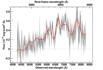
Figure 50: The SNIa 06D4ba_1280 spectrum measured at $z=0.70$ with a phase of 9.2 days. A Sd(2) host model has been subtracted.

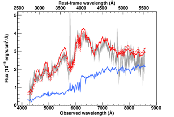
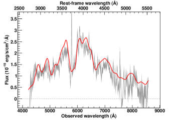
Figure 51: The SNIa 06D4bo_1280 spectrum measured at $z=0.552$ with a phase of 1.0 days. A S0-Sb host model has been subtracted.

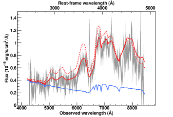
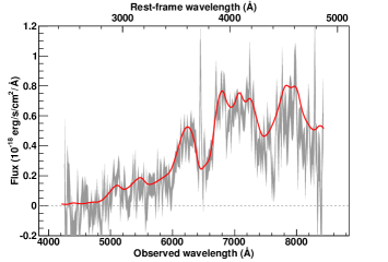
Figure 52: The SNIa 06D4bw_1279 spectrum measured at $z=0.732$ with a phase of 5.8 days. A Sa(1) host model has been subtracted.

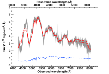
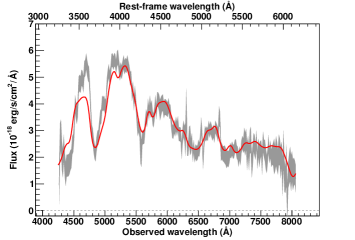
Figure 53: The SNIa 06D4gs_1358 spectrum measured at $z=0.31$ with a phase of -4.2 days. A E(1) host model has been subtracted.

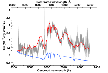
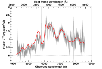
Figure 54: The SNIa 06D4jh_1413 spectrum measured at $z=0.566$ with a phase of 3.7 days. A Sd(2) host model has been subtracted.

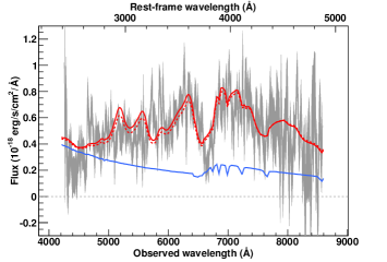
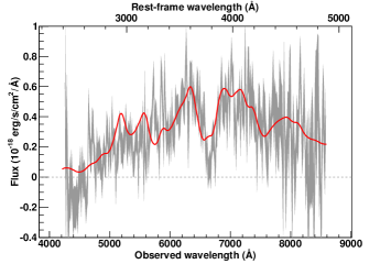
Figure 55: The SNIa$\star$ 06D4jt_1418 spectrum measured at $z=0.76$ with a phase of 2.9 days. A Sd(1) host model has been subtracted.

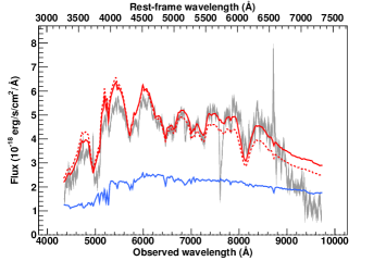
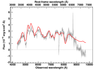
Figure 56: The SNIa 07D1ab_1483 spectrum measured at $z=0.328$ with a phase of -0.2 days. A E(1) host model has been subtracted.

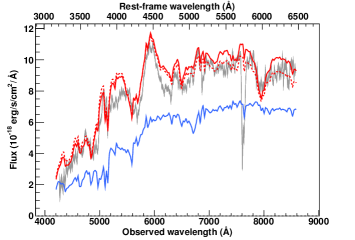
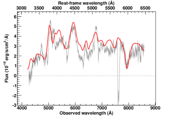
Figure 57: The SNIa 07D1ad_1484 spectrum measured at $z=0.297$ with a phase of 6.9 days. A S0(12) host model has been subtracted.

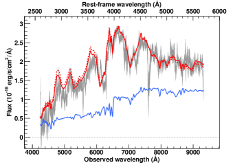
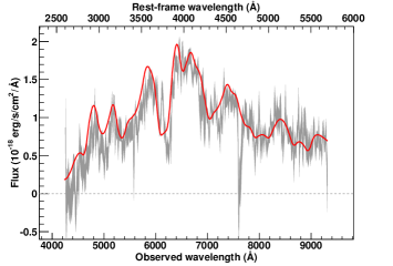
Figure 59: The SNIa 07D1bl_1707 spectrum measured at $z=0.636$ with a phase of 2.0 days. A E(2) host model has been subtracted.

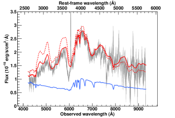
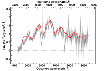
Figure 61: The SNIa 07D1bu_1711 spectrum measured at $z=0.626$ with a phase of -2.8 days. A Sd(5) host model has been subtracted.

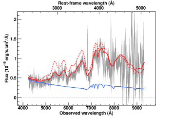
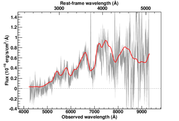
Figure 63: The SNIa$\star$ 07D1ca_1719 spectrum measured at $z=0.835$ with a phase of 1.4 days. A Sa(1) host model has been subtracted.

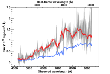
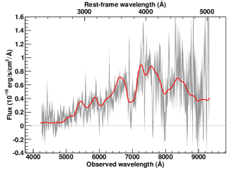
Figure 64: The SNIa 07D1cc_1719 spectrum measured at $z=0.853$ with a phase of 1.2 days. A Sa-Sb host model has been subtracted.

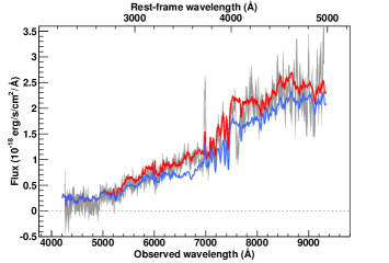
Figure 65: The SNIa$\star$ 07D1cd_1724 spectrum measured at $z=0.873$ with a phase of 4.1 days. A S0-Sa host model has been subtracted.

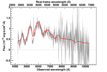
Figure 66: The SNIa 07D1cf_1723 spectrum measured at $z=0.500$ with a phase of -8.4 days. A E(1) host model has been subtracted.

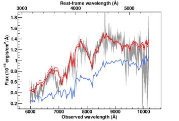
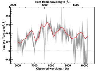
Figure 67: The SNIa 07D2aa_1487 spectrum measured at $z=0.899$ with a phase of -1.9 days. A S0(12) host model has been subtracted.

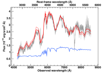
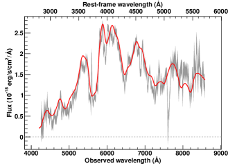
Figure 68: The SNIa 07D2ae_1485 spectrum measured at $z=0.501$ with a phase of 1.7 days. A S0(1) host model has been subtracted.

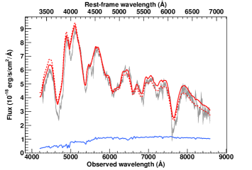
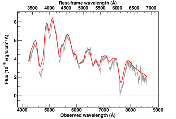
Figure 69: The SNIa 07D2ag_1485 spectrum measured at $z=0.25$ with a phase of -2.6 days. A S0(5) host model has been subtracted.

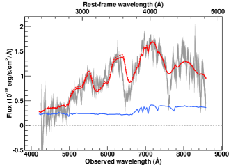
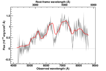
Figure 70: The SNIa 07D2ah_1486 spectrum measured at $z=0.780$ with a phase of -3.8 days. A S0(1) host model has been subtracted.

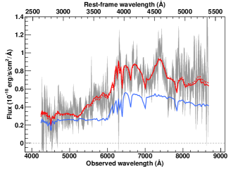
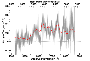
Figure 71: The SNIa$\star$ 07D2aw_1515 spectrum measured at $z=0.610$ with a phase of 10.0 days. A E(1) host model has been subtracted.

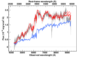
Figure 72: The SNIa 07D2bd_1510 spectrum measured at $z=0.572$ with a phase of 2.1 days. A Sa-Sb host model has been subtracted.

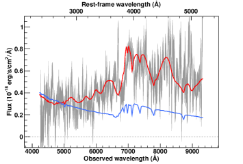
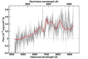
Figure 73: The SNIa$\star$ 07D2be_1510 spectrum measured at $z=0.793$ with a phase of 7.0 days. A Sc(1) host model has been subtracted.

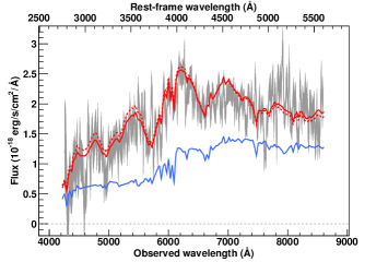
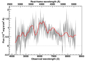
Figure 75: The SNIa 07D2bq_1518 spectrum measured at $z=0.535$ with a phase of -3.5 days. A E(1) host model has been subtracted.

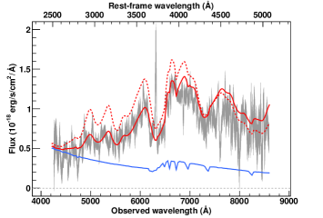
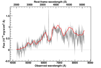
Figure 76: The SNIa 07D2cb_1536 spectrum measured at $z=0.694$ with a phase of 1.8 days. A Sd(1) host model has been subtracted.

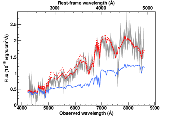
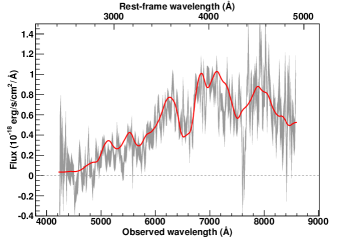
Figure 77: The SNIa$\star$ 07D2cq_1539 spectrum measured at $z=0.746$ with a phase of 1.1 days. A E(2) host model has been subtracted.

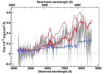
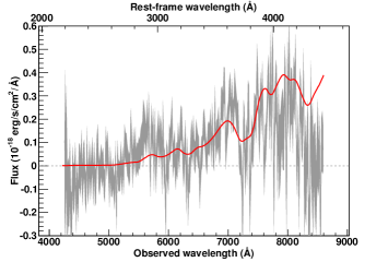
Figure 78: The SNIa$\star$ 07D2ct_1540 spectrum measured at $z=0.94$ with a phase of 1.9 days. A Sa-Sb host model has been subtracted.

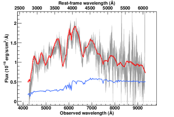
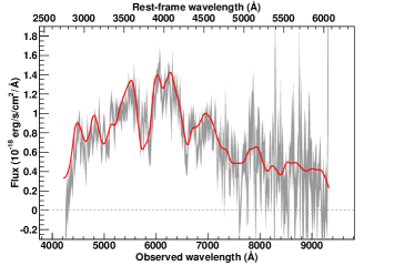
Figure 79: The SNIa 07D2du_1570 spectrum measured at $z=0.538$ with a phase of -1.4 days. A E(1) host model has been subtracted.

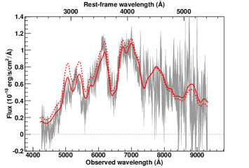
Figure 80: The SNIa 07D2fy_1596 spectrum measured at $z=0.72$ with a phase of 0.3 days. Best fit is obtained without galactic component.

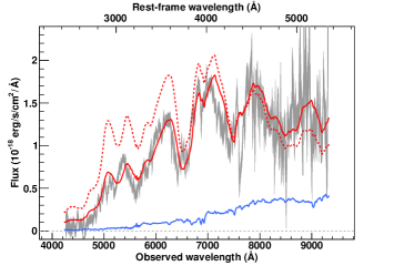
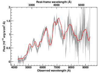
Figure 81: The SNIa 07D2fz_1596 spectrum measured at $z=0.743$ with a phase of -1.4 days. A E-S0 host model has been subtracted.

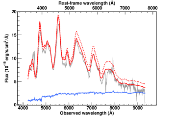
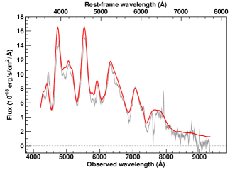
Figure 82: The SNIa 07D4aa_1630 spectrum measured at $z=0.207$ with a phase of 13.9 days. A Sb-Sc host model has been subtracted.

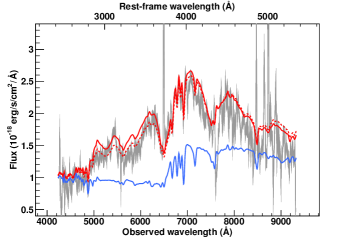
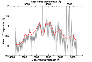
Figure 84: The SNIa$\star$ 07D4dp_1713 spectrum measured at $z=0.743$ with a phase of -1.8 days. A Sd(11) host model has been subtracted.

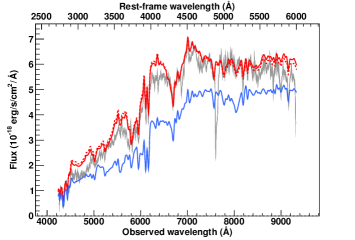
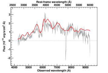
Figure 85: The SNIa 07D4dq_1713 spectrum measured at $z=0.554$ with a phase of 1.9 days. A E(3) host model has been subtracted.

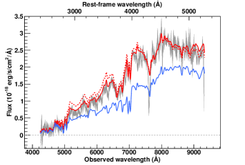
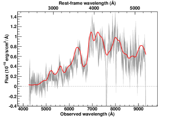
Figure 86: The SNIa 07D4dr_1713 spectrum measured at $z=0.772$ with a phase of 2.2 days. A E(4) host model has been subtracted.

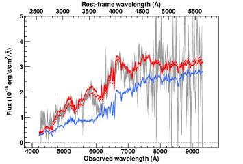
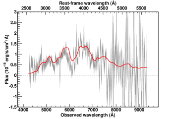
Figure 87: The SNIa 07D4ec_1722 spectrum measured at $z=0.653$ with a phase of -4.0 days. A Sa-Sb host model has been subtracted.

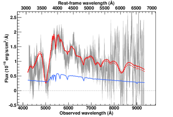
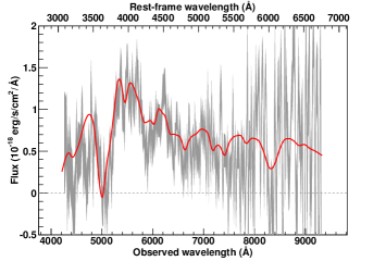
Figure 89: The SNIa 07D4ei_1725 spectrum measured at $z=0.37$ with a phase of -6.7 days. A S0(1) host model has been subtracted.