Abstract

Many predicted structured objects (e.g., sequences, matchings, trees) are evaluated using the F-score, alignment error rate (AER), or other multivariate performance measures. Since inductively optimizing these measures using training data is typically computationally difficult, empirical risk minimization of surrogate losses is employed, using, e.g., the hinge loss for (structured) support vector machines. These approximations often introduce a mismatch between the learner’s objective and the desired application performance, leading to inconsistency. We take a different approach: adversarially approximate training data while optimizing the exact F-score or AER. Structured predictions under this formulation result from solving zero-sum games between a predictor seeking the best performance and an adversary seeking the worst while required to (approximately) match certain structured properties of the training data. We explore this approach for word alignment (AER evaluation) and named entity recognition (F-score evaluation) with linear-chain constraints.

1 INTRODUCTION

Supervised structured prediction methods are prevalently used to predict sequences, alignments, or trees, for natural language processing (NLP) tasks  (Manning and Schütze, 1999; Lafferty et al., 2001; Och and Ney, 2003; Taskar et al., 2005c; Jurafsky and Martin, 2008; Finkel et al., 2008; Haghighi et al., 2009; Wang et al., 2013; Durrett and Klein, 2015). Unfortunately, inductively optimizing the precision, recall, F-score, alignment error rate (AER), or other multivariate evaluation measures of interest is intractable due to having many local optima—even for the simple 0-1 loss (Hoffgen et al., 1995) and the structured prediction extension: Hamming loss.

Existing approaches bypass these intractabilities by replacing the performance measure with a convex surrogate loss function for which optimization is tractable. This can be viewed as approximating the loss function and employing the exact training data. Minimizing the multivariate conditional logarithmic loss yields conditional random fields (CRFs) (Lafferty et al., 2001), and minimizing the structured hinge loss yields (structured) support vector machines (SVM) (Tsochantaridis et al., 2004). The latter method can integrate different multivariate performance measures into the hinge loss. However, the mismatch that using a hinge loss approximation introduces degrades predictive performance in both theory (i.e., inconsistency (Liu, 2007)) and practice.

We approach the task of structured predictions with multivariate performance measures by adversarially approximating the training data and using the exact evaluation measure in two important NLP tasks: named entity recognition evaluated using the F-score (§2.1) and word alignment evaluated using alignment error rate (§2.2). Our approach (§3) takes the form of a zero-sum game between a predictor player seeking label predictions that minimize expected multivariate loss and an adversary seeking to approximate the training data labels in limited ways based on structural relationships between the variables in a manner that maximizes expected multivariate loss. This generalizes previous methods for adversarially optimizing multivariate performance measures without structure (Wang et al., 2015) and adversarial structured prediction with chain structures and decomposable losses (Li et al., 2016). We investigate how these games can be solved efficiently using both exact and approximate constraint generation methods. Finally, we evaluate our approach in §4 with comparisons to CRFs and structured SVM methods.

2 BACKGROUND

Many important evaluation measures are multivariate, meaning they cannot be additively constructed by separately evaluating on each predicted variable. We focus on two measures: F-score and alignment error rate (AER) used in named entity recognition and word alignment tasks. We review these tasks before discussing existing methods for addressing them.

2.1 Named Entity Recognition

Identifying all occurrences of a type of entity in a sentence is often needed for natural language processing. Accuracy is often an inappropriate measure due to the relative infrequency of these occurrences. Instead, the F-score is commonly evaluated in named entity recognition (NER) (Finkel et al., 2005; Kim et al., 2003) and coreference resolution (Raghunathan et al., 2010; Lee et al., 2013) tasks. It is the harmonic mean of precision and recall of class $c$ based on predicted vector $\hat{\bf y}$ evaluated against ground truth vector ${\bf y}$:

$$F_{1}^{c}(\hat{\bf y},{\bf y})=\frac{2({\bf 1}_{\hat{\bf y}=c}\cdot{\bf 1}_{{\bf y}=c})}{|{\bf 1}_{\hat{\bf y}=c}|+|{\bf 1}_{{\bf y}=c}|},$$ (1)

where ${\bf 1}_{{\bf y}=c}$ is the binary vector that represents the occurrences of of $c$ in the gold standard sequence. ${\bf 1}_{\hat{\bf y}=c}$ is the binary vector that represents the existence of $c$ in the proposed sequence $\hat{\bf y}$.

Leveraging sequential structure improves performance in named entity recognition tasks (Finkel et al., 2005). This has previously been accomplished using conditional random fields (Lafferty et al., 2001) (§2.3). We seek a learning method that is better aligned with the F-score evaluation measure in this paper.

2.2 Word Alignment

Determining how words align between translated sentences is another important natural language processing task. The alignment error rate (AER) is a common evaluation measure for assessing machine translation quality (Cherry and Lin, 2006; Haghighi et al., 2009; Dyer et al., 2013; Kociskỳ et al., 2014). It generalizes the F-score for settings with more than binary-valued tags (Och and Ney, 2000). For example, an alignment task may contain three different kinds of tags between each pair of source and target words: a sure tag ($S$) for unambiguous alignments, a possible tag ($P$) for alignments that might exist or not, and a negative tag ($N$) for alignments that are neither $S$ nor $P$. For a gold standard sequence of alignments ${\bf y}$, and a proposed sequence of alignments $\hat{\bf y}$ from the system under evaluation, AER is defined as:

$$AER(\hat{\bf y},{\bf y})=1-\frac{{\bf 1}_{\hat{\bf y}=a}\cdot{\bf 1}_{{\bf y}=s}+{\bf 1}_{\hat{\bf y}=a}\cdot{\bf 1}_{{\bf y}=p}}{|{\bf 1}_{\hat{\bf y}=a}|+|{\bf 1}_{{\bf y}=s}|},$$ (2)

where $A$ is the proposed positive tag. $S$ alignments are also considered to be $P$ alignments ($S\subseteq P$) in this measure and it is evaluated accordingly. Figure 1 shows an example alignment task for an English-French translation.

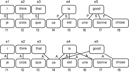
Figure 1: The gold standard sequence alignment (top) between English words $e_{i}$ and French words $f_{j}$ and the proposed sequence alignment ${\bf a}$ (bottom) with AER of $\frac{5}{13}$. Each complete alignment can be represented in sequence form as SNNNNNNNN$\ldots$NPSP and ANNNNNNNN$\ldots$NNNA for $(e_{1},f_{1}),(e_{1},f_{2}),\ldots,(e_{1},f_{8}),(e_{2},f_{1}),\ldots,(e_{5},f_{8})$ of the gold standard and proposed sequence alignments. Negative tags ($N$) are omitted in the figure for clarity.

2.3 Empirical Risk Minimization Approaches

In addition to being inherently multivariate, many key evaluation measures are also not concave (corresponding losses are non-convex). This makes it challenging to maximize these measures (or perform empirical risk minimization (ERM) for complementary loss functions): $\max_{\theta}\mathbb{E}_{{\bf Y},{\bf X}\sim\tilde{P},\hat{\bf Y}|{\bf X}\sim\hat{P}_{\theta}}\left[\text{score}(\hat{\bf Y},{\bf Y})\right]$ for training data distribution $\tilde{P}({\bf y},{\bf x})$ and predictive distribution $\hat{P}_{\theta}(\hat{\bf y}|{\bf x})$. Even the univariate prediction accuracy (zero-one loss) is a non-concave (non-convex) function of standard prediction model parameters, leading to an NP-hard optimization problem (Hoffgen et al., 1995). Instead, surrogate performance loss measures that upper bound the 0-1 loss/Hamming loss are employed: logistic regression and conditional random fields (CRFs) (Lafferty et al., 2001)—

$$\hat{P}_{\theta}({\bf y}|{\bf x})=\frac{e^{\sum_{t}{\theta}\cdot\Phi({\bf y}_{t-1},{\bf y}_{t},{\bf x}_{t})}}{\sum_{{\bf y}}e^{\sum_{t}{\theta}\cdot\Phi({\bf y}_{t-1},{\bf y}_{t},{\bf x}_{t})}},\text{ where: }$$ (3)

$$\theta=\operatorname*{arg\,min}_{\theta}\mathbb{E}_{{\bf X},{\bf Y}\sim\tilde{P}}\left[-\log\hat{P}_{\theta}({\bf Y}|{\bf X})\right]$$

—minimize the logarithmic loss (maximizing log-likelihood); the (structured) support vector machine (SVM) (Cortes and Vapnik, 1995; Tsochantaridis et al., 2004) and max-margin Markov networks (Taskar et al., 2004) minimize the hinge loss surrogate. The hinge loss $\xi_{i}$ grows linearly with the difference between the potential $\Phi({\bf x}^{(i)},{\bf y}^{(i)})$ of the gold standard label ${\bf y}^{(i)}$ and the best alternative label ${\bf y}^{\prime}$ when the gold standard is not better by at least the multivariate loss between ${\bf y}^{\prime}$ and ${\bf y}^{(i)}$, denoted $\Delta({\bf y}^{\prime},{\bf y}^{(i)})$:

$$\min_{\theta,\xi_{i}\geq 0}\sum_{i}\xi_{i}+\frac{\lambda}{2}||\theta||^{2}\text{ subject to: }\forall i,{\bf y}^{\prime}\in\boldsymbol{\mathcal{Y}},$$ (4)

$${\theta}\cdot[\Phi({\bf x}^{(i)},{\bf y}^{(i)})-\Phi({\bf x}^{(i)},{\bf y}^{\prime})]\geq\Delta({\bf y}^{\prime},{\bf y}^{(i)})-\xi_{i}.$$

Though the ability to incorporate multivariate loss functions is attractive, the hinge loss approximation leads to theoretical shortcomings, including a lack of Fisher consistency (Liu, 2007), meaning even if trained using the true distribution $P({\bf y},{\bf x})$ and an arbitrarily rich feature representation $\Phi$, predictions minimizing the multivariate loss are not guaranteed.

3 ADVERSARIAL STRUCTURED PREDICTION GAMES

We present a generalized adversarial formulation (§3.1) for prediction tasks with both multivariate performance measures and structured properties relating the predicted variables. We review a general constraint generation method for solving the resulting game problems efficiently (§3.2) and establish its applicability to the AER performance measure over matchings (§3.3), more restrictive bipartite matching (§3.4), and F-measure with chain constraints (§3.5).

3.1 Adversarial Game Formulation

We construct structured predictors for specific performance measures by taking an adversarial philosophy with respect to inductive uncertainty. For a particular performance measure, we seek the predictor that is robust to the worst-case label approximation that still matches structural properties measured on training data or other structural constraints on the predicted variables from the domain. Mathematically, this takes the form of a zero-sum game  (von Neumann and Morgenstern, 1947) between two players: player $\hat{\bf Y}$ who maximizes the expected score between the two players’ structured choices, and player $\check{\bf Y}$ who approximates the training data in a manner that minimizes the expected score while also residing within the constraint set $\Xi$, which is defined as: $\mathbb{E}_{{\bf X}\sim\tilde{P},\check{\bf Y}|{\bf X}\sim\check{P}}\left[\Phi({\bf X},\check{\bf Y})\right]=\mathbb{E}_{{\bf Y},{\bf X}\sim\tilde{P}}\left[\Phi({\bf X},{\bf Y})\right]$:

$$\max_{\hat{P}(\hat{\bf y}|{\bf x})}\min_{\check{P}(\check{\bf y}|{\bf x})\in\Xi}\mathbb{E}_{{\bf X}\sim\tilde{P},\hat{\bf Y}|{\bf X}\sim\hat{P},\check{Y}|{\bf X}\sim\check{P}}\left[\text{score}(\hat{\bf Y},\check{\bf Y})\right]$$ (5)

$$=\max_{\theta}\bigg{\{}\mathbb{E}_{{\bf Y},{\bf X}\sim\tilde{P}}[\psi({\bf X},{\bf Y})]$$

$$+\sum_{{\bf x}\in\boldsymbol{\mathcal{X}}}\tilde{P}({\bf x})\!\!\min_{\check{P}(\check{\bf y}|{\bf x})}\max_{\hat{P}(\hat{\bf y}|{\bf x})}\Big{[}\underbrace{\text{score}(\hat{\bf Y},\check{\bf Y})-\psi({\bf x},\check{\bf Y})}_{{\boldsymbol{S}}^{\prime}_{\hat{\bf y},\check{\bf y}}}\Big{]}\bigg{\}},$$ (6)

where the parameters $\theta$ for the Lagrangian term $\psi({\bf x},\check{\bf y})=\theta\cdot\Phi({\bf x},\check{\bf y})$, are a learned weight vector, and $\Phi({\bf x},\check{\bf y})$ are the features characterizing the relationship between ${\bf x}$ and $\check{\bf y}$.

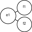
Figure 2: Alignment task with one source and two target words.

For example, the score matrix (Eq. (5)) for the $(1-AER)$ game for a simple setting with one source word (e1) and two target words (f1, f2) from Figure 2 is expanded to ${\boldsymbol{S}}^{\prime}_{\hat{\bf y},\check{\bf y}}$, as shown in Table 1, with Lagrangian terms, $\psi(\check{\bf y})$, that enforce the constraint requirement, $\check{P}(\check{\bf y}|{\bf x})\in\Xi$, by motivating the adversary to produce features that are similar to those of the training data set. The predictor chooses (a distribution of) {A, N} tags for the pair of edges, while the adversary chooses (a distribution of) {S, P, N} tags that also resides within the set $\Xi$. This corresponds to the game in Eq. (6), which can be expressed as a linear program. Estimating game parameters $\theta$ is a convex optimization problem, which can be solved using existing convex optimization methods (e.g., AdaDelta, L-BFGS).

Table 1: The ($1-AER$) game matrix ${\boldsymbol{S}}^{\prime}_{\hat{\bf y},\check{\bf y}}$.

	NN	NA	AN	AA
NN	$1-\psi(NN)$	$0-\psi(NN)$	$0-\psi(NN)$	$0-\psi(NN)$
NP	$1-\psi(NP)$	$1-\psi(NP)$	$0-\psi(NP)$	$\frac{1}{2}-\psi(NP)$
NS	$0-\psi(NS)$	$1-\psi(NS)$	$0-\psi(NS)$	$\frac{2}{3}-\psi(NS)$
PN	$1-\psi(PN)$	$0-\psi(PN)$	$1-\psi(PN)$	$\frac{1}{2}-\psi(PN)$
PP	$1-\psi(PP)$	$1-\psi(PP)$	$1-\psi(PP)$	$1-\psi(PP)$
PS	$0-\psi(PS)$	$1-\psi(PS)$	$\frac{1}{2}-\psi(PS)$	$1-\psi(PS)$
SN	$0-\psi(SN)$	$0-\psi(SN)$	$1-\psi(SN)$	$\frac{2}{3}-\psi(SN)$
SP	$0-\psi(SP)$	$\frac{1}{2}-\psi(SP)$	$1-\psi(SP)$	$1-\psi(SP)$
SS	$0-\psi(SS)$	$\frac{2}{3}-\psi(SS)$	$\frac{2}{3}-\psi(SS)$	$1-\psi(SS)$

One key advantage of the adversarial approach over structured prediction methods based on the hinge loss is its Fisher consistency guarantee (Li et al., 2016). Given the full data distribution, $P({\bf y},{\bf x})$, and an arbitrarily rich feature representation, the adversary is constrained by the set $\Xi$ to exactly match the conditional distribution of the data, $\check{P}({\bf y}|{\bf x})=P({\bf y}|{\bf x})$. Equation (5) then reduces to:

$$\max_{\hat{P}(\hat{\bf y}|{\bf x})}\mathbb{E}_{{\bf X}\sim{P},\hat{\bf Y}|{\bf X}\sim\hat{P},{\bf Y}|{\bf X}\sim P}\left[\text{score}(\hat{\bf Y},{\bf Y})\right],$$ (7)

which is the optimizer of the evaluation measure, $\text{score}(\hat{\bf y},{\bf y})$, on the full distribution of data.

3.2 Double Oracle Method

Unfortunately, the games for these multivariate settings grow exponentially in size with the number of variables. For example, the $1-AER$ game for the sequence alignment task of Figure 1 has $5\cdot 8$ word pairs, yielding $3^{5\cdot 8}$ sequence choices for the adversary, $2^{5\cdot 8}$ sequence choices for the predictor player, and a game size of $(2\cdot 3)^{5\cdot 8}\approx 1.3\cdot 10^{31}$. Thus, explicitly constructing and solving the game matrix is computationally impractical even for small alignment tasks.

We use the double oracle method (McMahan et al., 2003) to obtain the equilibrium solution to the adversarial prediction game without explicitly constructing the game matrix. It iteratively adds a new sequence (for one player at a time) in response to the opponent’s current equilibrium distribution over sequences obtained from solving a zero-sum game with the sets of current sequences. This continues until adding more sequences no longer benefits either player, guaranteeing a Nash equilibrium for the original game.

The double oracle game solver is a central component of the our approach. Its returned equilibrium distributions are used to compute the gradients needed for learning the model parameters, $\theta$. The zero-sum game solver used as a sub-routine of the double oracle method is implemented using linear programming (Ferguson, 2014), with different linear program solvers available (Optimization, 2014; Berkelaar et al., 2004). The key remaining problem—also a required subroutine of the double oracle method—is to efficiently find each player’s best response:

$$\hat{\bf y}^{*}=\operatorname*{arg\,max}_{\hat{\bf y}}\mathbb{E}_{\check{\bf Y}|{\bf x}\sim\check{P}}[\text{score}(\hat{\bf y},\check{\bf Y})-\psi(\check{\bf Y})],$$ (8)

$$\check{\bf y}^{*}=\operatorname*{arg\,min}_{\check{\bf y}}\mathbb{E}_{\hat{\bf Y}|{\bf x}\sim\hat{P}}[\text{score}(\hat{\bf Y},\check{\bf y})-\psi(\check{\bf y})].$$ (9)

The difficulty depends on both the loss function being considered and the constraints imposed on the adversary. We efficiently solve this best response problem under structured constraints for alignment error rate and F-score with chain structured constraints in the next sections.

3.3 Best Response for Alignment Error Rate

Under our approach for $1-AER$, the two players are: ${\bf y}\in\mathbb{Y}$, which adversarially approximates the gold standard alignment distribution; and ${\bf a}\in\mathbb{A}$, which maximizes $1-AER$ (hence, minimizes AER), where $\mathbb{A}$ and $\mathbb{Y}$ are the domain of ${\bf a}$ with a distribution $Q(\mathbb{A})$, and ${\bf y}$ with a distribution $Q(\mathbb{Y})$ respectively. For a sequence of alignments of length $n$, the objective of finding the best responses ${\bf a}^{*}$ (Eq. (8)) and ${\bf y}^{*}$ (Eq. (9)) are:

$${\bf a}^{*}=\operatorname*{arg\,max}_{{\bf a}\in\mathbb{A}}\!\!\!\!{\sum_{{\bf y}\in{\{0,S,P\}}^{n}}}\!\!\!\!\!q({\bf y})\left[1-AER({\bf a},{\bf y})-\psi({\bf y})\right],$$ (10)

$${\bf y}^{*}=\operatorname*{arg\,min}_{{\bf y}\in\mathbb{Y}}\!\!\!\!{\sum_{{\bf a}\in{\{0,A\}}^{n}}}\!\!q({\bf a})[1-AER({\bf a},{\bf y})-\psi({\bf y})].$$ (11)

We focus first on the adversary’s best response (Equation (11)), which must incorporate the Lagrangian potential term, $\psi({\bf y})$. For the choice of alignment $y^{*}$, we separate the choices among all possible numbers of $S$ tags, $k={0,...,n}$, for the alignment sequence of length $n$, and denote these sets as $\mathbb{Y}^{(k)}$. The best choice of a certain $k$ is rewritten as follows, where $a_{i}$ is the notational shorthand of the indicator function $I(a_{i}=A)$, and $y_{si}=I(y_{i}=S),y_{ri}=I(y_{i}=P,y_{i}\neq S)$; the number of $A$ tags in the alignment is $\alpha=\sum_{i=1}^{n}a_{i}$:

$${\bf y}^{(k)^{*}}=\operatorname*{arg\,min}_{{\bf y}\in\mathbb{Y}^{(k)}}\sum_{{\bf a}\in{\{0,A\}}^{n}}q({\bf a})\bigg{(}\frac{\sum_{i=1}^{n}(2a_{i}y_{si}+a_{i}y_{ri})}{\alpha+k}-\sum_{i=1}^{n}\psi_{i}(y_{i})\bigg{)}$$

$$=\operatorname*{arg\,min}_{{\bf y}\in\mathbb{Y}^{(k)}}\!\!\!\!\!\!\!\sum_{\;\;\;{\bf a}\in{\{0,A\}}^{n}}\!\!\!\!q({\bf a})\sum_{i=1}^{n}\bigg{(}\frac{a_{i}(2y_{si}+y_{ri})}{\alpha+k}-\psi_{i}^{(S)}y_{si}-\psi_{i}^{(R)}y_{ri}\bigg{)}$$ (12)

$$=\operatorname*{arg\,min}_{{\bf y}\in\mathbb{Y}^{(k)}}\sum_{i=1}^{n}y_{si}\underbrace{2\sum_{\alpha=1}^{n}\left(\frac{q_{i\alpha}}{\alpha+k}-\psi_{i}^{(S)}\right)}_{f_{sik}}+\sum_{i=1}^{n}y_{ri}\underbrace{\sum_{\alpha=1}^{n}\left(\frac{q_{i\alpha}}{\alpha+k}-\psi_{i}^{(R)}\right)}_{f_{rik}}.$$

Here, in Equation (12), $q_{i\alpha}$ is the marginal probability that alignment $a$ has $|a_{S}|=\alpha$ and $a_{i}=S$ (i.e., the number of $S$ tags equals to $\alpha$, and the $i$-th position is $S$). We separate the Lagrangian potential $\psi$ into two terms: $\psi^{(S)}$ for $S$ tags, $\psi^{(R)}$ for $P$ tags that are not also $S$ tags. To get the permutation that minimizes this equation, for tag $S$ at position $i$ we pay $f_{sik}$, for tag $P$ we pay $f_{rik}$, and for tag $N$ we pay $0$. Without the ${\bf y}\in\mathbb{Y}^{(k)}$ constraint, to compute the minimum, all that we need to do is finding the smallest of these three terms for each $i$. With the constraint, we have to set exactly $k$ tags to $S$, so we choose the $k$ positions where the $f_{sik}$ cost exceeds the best alternative, $\min(f_{rik},0)$, by as little as possible. Thus, we sort $(f_{sik}-\min(f_{rik},0))$ in ascending order, set the top $k$ positions to $S$, $P$, or $N$ accordingly. The detailed algorithm is shown as Algorithm 1.

Algorithm 1 AER Maximizer

1:procedure AerMax($Q(\mathbb{A})$, $\psi^{(S)}$, $\psi^{(R)}$)

2:  define vector $W_{0}$ with element $w_{i0}=\frac{1}{i}$

3:  define matrix $W$ with element $w_{ik}=\frac{1}{i+k}$, where $i,k\in\{1,...,n\}$

4:  compute vector $F_{0}=QW_{0}-\psi^{(R)}$

5:  compute matrix $F_{S}=2QW-\psi^{(S)^{T}}{\bf 1}^{n}$

6:  compute matrix $F_{R}=QW-\psi^{(R)^{T}}{\bf 1}^{n}$

7:  set positions of $y^{(0)^{*}}$ with $f_{i0}<0$ to ‘$P$’

8:  $\mathbb{E}_{(1-AER)^{\prime}}({\bf y}^{(0)^{*}})=\sum_{i=1}^{n}\min(f_{i0},0)$

9:  for $k=1$ to $n$ do

10:   find ${\bf y}^{(k)^{*}}$ by:

11:   sort $f_{ik}=f_{sik}-\min(f_{rik},0)$ in asc. order

12:   set positions with top $k$’s $f_{ik}$ to ‘$S$’

13:   set each rest position $i$ to ‘$P$’ if $f_{rik}<0$

14:   $\mathbb{E}_{(1-AER)^{\prime}}({\bf y}^{(k)^{*}})=\sum_{i=1}^{n}y_{si}f_{sik}+y_{ri}f_{rik}$   

15:  return ${\bf y}^{*}=\operatorname*{arg\,min}_{{\bf y}^{(k)^{*}}}{\mathbb{E}_{(1-AER)^{\prime}}({\bf y}^{(k)^{*}})}$

The best response for the AER minimizer is simpler to obtain since the Lagrangian terms $\psi({\bf y})$ are invariant to the choice of alignment ${\bf a}^{*}$. The approach of (Dembczynski et al., 2011) can be used after replacing $F=PW$ with $F^{\prime}=Q_{S}W_{S}+Q_{P}W_{P}$, where matrix $Q_{S}$ is the marginal probability for $S$ tag, $Q_{P}$ is for $P$ tag, and permutation matrices $W_{S}$, $W_{P}$ are for $S$ and $P$ respectively, where each element (with index $i,k$) in the matrix $w_{S}^{ik}=\frac{2}{i+k}$, and $w_{P}^{ik}=\frac{1}{i+k-1}$.

3.4 Best Response for Bipartite Matching

Following Taskar et al. (2005b)’s modeling of the AER task as a maximum weighted bipartite matching problem using additive cost-sensitive losses (Cormen et al., 2001), we develop a bipartite best response for our adversarial approach. The best response problems are:

$${\bf a}^{*}=\operatorname*{arg\,max}_{{\bf a}\in\mathbb{A}}\!\!\!\!{\sum_{{\bf y}\in{\{0,S,P\}}^{n}}}\!\!\!\!\!q({\bf y})\sum_{i}\left[1-C({a}_{i},{y}_{i})-\psi({y}_{i})\right],$$

$${\bf y}^{*}=\operatorname*{arg\,min}_{{\bf y}\in\mathbb{Y}}\!\!\!\!{\sum_{{\bf a}\in{\{0,A\}}^{n}}}\!\!q({\bf a})\sum_{i}[1-C(a_{i},y_{i})-\psi(y_{i})],$$

where each ${\bf a}$ or ${\bf y}$ must also be a valid bipartite matching, and $C(\cdot,\cdot)$ is a cost function. The best responses can be computed using widely used maximum weight bipartite matching algorithms (Lawler, 2001) by incorporating Lagrangian potentials and expected losses as edge weights and an integer linear program exactly using the integral solution of a linear program relaxation.

3.5 Best Response for Linear-chain F-score

Exact Best Responses:

We consider the F-score for a particular class $C$ and define two players in the zero-sum game: player $\hat{\bf Y}$ makes predictions that maximizes F-score, and player $\check{\bf Y}$ adversarially approximates the evaluation distribution. For each set of adversarial sequences $\mathbb{Y}$, and its distribution $P(\mathbb{Y})$, the best response should be found efficiently:

$$\hat{\bf y}^{*}=\operatorname*{arg\,max}_{\hat{\bf y}\in\mathbb{\hat{Y}}}{\sum_{\check{\bf y}}}\;p(\check{\bf y})[F_{1_{C}}(\hat{\bf y},\check{\bf y})-\psi(\check{\bf y})],$$ (13)

$$\check{\bf y}^{*}=\operatorname*{arg\,min}_{\check{\bf y}\in\mathbb{\check{Y}}}{\sum_{\hat{\bf y}}}\;p(\hat{\bf y})[F_{1_{C}}(\hat{\bf y},\check{\bf y})-\psi(\check{\bf y})].$$ (14)

Algorithm 2 Linear-Chain F-score Minimizer

1:procedure LCFM($P(\mathbb{\hat{Y}})$, $\psi^{u}$, $\psi^{b}$, $C$)

2:  define matrix $W$ with element $w_{tk}=\frac{1}{t+k}$

3:  compute matrix $F=2PW$ $\triangleright$ element $f_{tk}$

4:  $[\check{{\bf y}}^{(0)^{*}},\mathbb{E}_{F_{1}}(\check{{\bf y}}^{(0)^{*}})]$$\leftarrow$ MSUM(START, 1, 0, 0, F)

5:  $\mathbb{E}_{F_{1}}(\check{{\bf y}}^{(0)^{*}})\leftarrow\mathbb{E}_{F_{1}}(\check{{\bf y}}^{(0)^{*}})-p_{0}$

6:$\triangleright$ $p_{0}$ is the marginal probability that $|\hat{y}_{C}|=0$

7:  for $k\leftarrow 1\dots n$ do

8:   $[\check{{\bf y}}^{(k)^{*}},\mathbb{E}_{F_{1}}(\check{{\bf y}}^{(k)^{*}})]\leftarrow$MSUM(START,$1,k,k,F$)   

9:  $\mathbb{E}_{F_{1}}(\check{{\bf y}}^{*})\leftarrow\max_{k}(\mathbb{E}_{F_{1}}(\check{{\bf y}}^{(k)^{*}}))$

10:  $\check{{\bf y}}^{*}\leftarrow\operatorname*{arg\,max}_{\check{{\bf y}}^{(k)^{*}}}\mathbb{E}_{F_{1}}(\check{{\bf y}}^{(k)^{*}})$

11:  return $[\check{{\bf y}}^{*},-\mathbb{E}_{F_{1}}(\check{{\bf y}}^{*})]$

12:procedure MSUM($c_{t-1},t,r,k,F$)

13:  if $[\check{{\bf y}}^{*},\mathbb{E}_{F_{1}}(\check{{\bf y}}^{*})]$=cache($c_{t-1},t,r,k$) exists then

14:   return $[\check{{\bf y}}^{*},\mathbb{E}_{F_{1}}(\check{{\bf y}}^{*})]$   

15:  if $t>n$ and $r>0$ then return $[\Phi,-\infty]$

16:  else if $t>n$ and $r\leq 0$ then return $[\Phi,0]$   

17:  $[\check{{\bf y}}^{*},\mathbb{E}_{F_{1}}(\check{{\bf y}}^{*})]\leftarrow[\Phi,-\infty]$

18:  for $c_{t}\in\mathbb{C}$ do

19:   $\psi(c_{t})\leftarrow\psi_{t}^{u}(c_{t})+\psi_{t}^{b}(c_{t-1},c_{t})$

20:   $f\leftarrow f_{tk}\times I(c_{t}=C)\times I(k>0)$

21:   if $r>0\,|\,c_{t}\neq C$ then

22:     $r^{\prime}\leftarrow r-I(c_{t}=C)$

23:     $[\check{{\bf y}}^{c_{t}},\mathbb{E}_{F_{1}}(\check{{\bf y}}^{c_{t}})]\leftarrow$ MSUM($c_{t},t+1,r^{\prime},k,F$)

24:     if $\mathbb{E}_{F_{1}}(\check{{\bf y}}^{*})<\psi(c_{t})-f+\mathbb{E}_{F_{1}}(\check{{\bf y}}^{c_{t}})$ then

25:      $\mathbb{E}_{F_{1}}(\check{{\bf y}}^{*})\leftarrow\psi(c_{t})-f+\mathbb{E}_{F_{1}}(\check{{\bf y}}^{c_{t}})$

26:      $\check{{\bf y}}^{*}\leftarrow c_{t}\oplus\check{{\bf y}}^{c_{t}}$           

27:  cache($c_{t-1},t,r,k$) $\leftarrow[\check{{\bf y}}^{*},\mathbb{E}_{F_{1}}(\check{{\bf y}}^{*})]$

28:  return cache($c_{t-1},t,r,k$)

Chain structures permit two types of features: unigram $\Phi^{u}(\mathbf{x}_{t},y_{t})$, and bigram $\Phi^{b}(\mathbf{x}_{t},y_{t-1},y_{t})$. We encode the linear-chain structure information in the weight vectors (i.e., Lagrange multipliers in Equation (14)). For example, suppose we have $m$ classes $C_{t}\in\mathbb{C}=\{C^{1},...,C^{m}\}$ in the data set. Then each distinct consecutive pair of classes $(C_{t-1},C_{t})$ has its own weight vector $\mathbf{\theta}^{b}(C_{t-1},C_{t})$, for a total number of pairs and weight vectors $m^{2}$. An optional START tag can be added in front of a sequence, forming $m$ additional pairs $({\it START},C_{1})$ (and corresponding weight vectors). Besides these pair vectors that accommodate bigram features, each class also has a separate weight vector $\mathbf{\theta}^{u}(C_{t})$ for unigram features in our model. So in total, we use $m$ unigram feature vectors, and $m^{2}(+m)$ bigram feature vectors to capture the linear chain information.

From Equation (13), we can see that the Lagrange potentials $\psi(\check{\bf y})$ are related to the choice of $\check{\bf y}$ only, and because the binary nature of the F-score of a specific target class (Jurafsky and Martin, 2008), the GFM algorithm (Dembczynski et al., 2011) can be applied directly to the binarized sequences for the target.

For the adversary’s best response, we rewrite Equation (14) for a particular target class $C$ by considering the total number of target class in $\hat{\bf y}$ and $\check{\bf y}$ sequence as $\hat{k}$ and $\check{k}$ respectively, as follows:

$$\check{{\bf y}}^{*} =\operatorname*{arg\,min}_{\check{{\bf y}}^{(\check{k})^{*}}}{\sum_{\hat{{\bf y}}}}p(\hat{{\bf y}})\bigg{\{}\frac{2\sum_{t=1}^{n}\hat{y}_{Ct}\check{y}_{Ct}}{\hat{k}+\check{k}}$$

$$\qquad-\sum_{t=1}^{n}\left[\psi_{t}^{u}(\check{y}_{t})+\psi_{t}^{b}(\check{y}_{t-1},\check{y}_{t})\right]\bigg{\}},$$

$$\check{{\bf y}}^{(\check{k})^{*}} =\operatorname*{arg\,min}_{\check{{\bf y}}\in\mathbb{\check{Y}}^{(\check{k})}}{\sum_{t=1}^{n}\Bigg{\{}\left(\sum_{\hat{{\bf y}}}p(\hat{{\bf y}})\frac{2\hat{y}_{Ct}\check{y}_{Ct}}{\hat{k}+\check{k}}\right)}$$

$$\qquad\qquad-\left[\psi_{t}^{u}(\check{y}_{t})+\psi_{t}^{b}(\check{y}_{t-1},\check{y}_{t})\right]\Bigg{\}}$$

$$=\operatorname*{arg\,max}_{\check{{\bf y}}\in\mathbb{\check{Y}}^{(\check{k})}}\sum_{t=1}^{n}\bigg{\{} \psi_{t}^{u}(\check{y}_{t})+\psi_{t}^{b}(\check{y}_{t-1},\check{y}_{t})-\underbrace{{\sum_{\hat{k}=1}^{n}}\frac{2p^{C}_{t\hat{k}}}{\hat{k}+\check{k}}}_{f_{t\check{k}}}\check{y}_{Ct}\bigg{\}},$$ (15)

where $\hat{y}_{Ct}=I(\hat{y}_{t}=C)$, $\check{y}_{Ct}=I(\check{y}_{t}=C)$, $\hat{k}=\sum_{t=1}^{n}\hat{y}_{Ct}$, $\check{k}=\sum_{t=1}^{n}\check{y}_{Ct}$ and $p^{C}_{t\hat{k}}$ is the marginal probability that $|\hat{y}_{C}|=\hat{k}$ and $\hat{y}_{t}=C$.

The difficulty of solving Eq. (15) comes from the Lagrange potential term $[\psi_{t}^{u}(\check{y}_{t})+\psi_{t}^{b}(\check{y}_{t-1},\check{y}_{t})]$ in the linear-chain structure. To solve this problem efficiently, we propose a dynamic programming algorithm, for the particular class $C$, Linear-Chain F-score Minimizer (LCFM) in Algorithm 2. The MSUM subroutine computes the sum in Equation (15) via a backward pass with the following recurrence relation for $\check{k}$ instances of class $C$ tags in sequence $\check{\bf y}$:

$$\beta^{\check{k}}(c_{t-1},t,r)= \begin{cases}0&\!\!t=0\\ \max_{c_{t}}\{\beta^{\check{k}}(c_{t},t+1,r-I(c_{t}=C))&\!\!t>0\\ +\psi(c_{t-1},c_{t})-f_{t\check{k}}\times I(c_{t}=C)\}.\end{cases}$$

Looping through subroutines of MSUM for each of the $n$ values of $\check{k}$, i.e., number of target tags in the best response sequence, can be accomplished in $\mathcal{O}(m^{2}n^{3})$ time, which characterizes the overall complexity of the algorithm.

Approximate Best Responses:

To overcome this cubic complexity, we employ an approximation method for F-score over the linear-chain structure using the cost sensitive approach proposed by Parambath et al. (2014). For different costs of false negatives chosen as $\delta_{+}\in\{2-w,w\in\{0.1,0.2,\dots,1\}\}$ against false positive cost of $\delta_{-}\in\{w,w\in\{0.1,0.2,\dots,1\}\}$, we find the best response over the linear chain by a Viterbi forward pass in $O(nm^{2})$, i.e for the adversary we compute:

$$\alpha^{w}(c_{t})= \begin{cases}0&\!\!\!\!\!\!\!\!t=0\\ \max_{c_{t-1}}\{\alpha^{w}(c_{t-1})+\psi(c_{t-1},c_{t})\}&\!\!\!\!\!\!\!\!t>0\\ \;+I(c_{t}=C)(1-P^{C}_{t})\delta^{w}_{-}+I(c_{t}\neq C)P^{C}_{t}\delta^{w}_{+}\end{cases}$$ (16)

where $P^{C}_{t}$ is the marginal probability that $\check{\mathbf{y}}_{t}=C$.

The algorithm finds the approximated best response by calling the dynamic programming subroutine for different values of $w$ and chooses the sequence with the lowest F-score a posteriori. For the maximizer player, in absence of Lagrangian potentials, choosing the best tag at each position becomes an independent binary decision (target vs. non-target tag) which can be accomplished in $O(n)$. We transform the range of Lagrangian potentials in (16) to $[-1,1]$ in order to better match the range of cost terms.

4 EXPERIMENTS AND RESULTS

We evaluate our approach against a maximum margin structured prediction model / SSVM (Taskar et al., 2005c; Tsochantaridis et al., 2004) for alignment error rate and conditional random field (CRF) for linear-chain F-score. Since the maximum margin method’s implementation is not available, we implemented it ourselves following the algorithm description (Taskar et al., 2005a, c, b). We use the Stanford Named Entity Recognizer’s CRF implementation (Finkel et al., 2005) in our experiments.

We use the NAACL 2003 Hansards data (Mihalcea and Pedersen, 2003) for the AER task. It contains 1,470,000 unlabeled sentence pairs, 447 labeled pairs, and a separate validation set of 37 labeled pairs. We experiment with translation from English to French, following the same setting as Taskar et al. (2005c) and Cherry and Lin (2006). We use first 100 English-French sentence pairs from the original labeled data as training examples, the remaining 347 sentence pairs as test examples, and the same 37 validation pairs as validation examples. Since the features described in Taskar et al. (2005c) are not available, we duplicate them with our best efforts.

We train the maximum margin structured model ($SSVM$), and our adversarial approach (ADV) with maximum weight bipartite matching ($ADV_{bip}$), and without bipartite matching constraints for AER ($ADV_{aer}$) using those features extracted from the training data set. Also, following the same setting as Taskar et al. (2005c), we include GIZA++’s unsupervised prediction from the $1^{5}H^{5}3^{3}4^{3}$ training scheme (Och and Ney, 2003) as an additional feature. We select $\ell_{2}$ regularization values using performance on the validation data set.

Table 2: AER of different models.

Model	Valid	Test
$SSVM$	13.98%	13.34%
$MPG_{bip}$	15.82%	14.52%
$MPG_{aer}$	6.97%	7.28%

Table 3: $F_{1}$ scores of $CRF$ and $MPG_{f_{1}}$ on ‘testa’ (top) and ‘testb’ (bottom).

Dataset		testa
		$CRF$	$ADV_{f_{1}}$	$ADV^{\approx}_{f_{1}}$
conll300	PER	17.88	29.64	29.64
	LOC	30.94	47.40	47.40
	ORG	7.19	15.74	15.74
	MISC	16.22	19.51	19.51
conll1000	PER	78.68	85.42	85.42
	LOC	80.00	78.63	78.63
	ORG	58.24	59.39	59.39
	MISC	62.30	67.08	67.08
conll3000	PER	85.72	88.97	88.97
	LOC	85.74	85.38	85.38
	ORG	75.69	76.34	76.34
	MISC	78.82	81.04	81.04

Dataset		testb
		$CRF$	$ADV_{f_{1}}$	$ADV^{\approx}_{f_{1}}$
conll300	PER	40.00	44.68	44.68
	LOC	52.10	66.34	66.34
	ORG	14.16	19.04	19.04
	MISC	30.43	35.21	35.21
conll1000	PER	76.36	83.21	83.21
	LOC	76.65	76.81	76.81
	ORG	61.14	61.73	61.73
	MISC	59.28	66.06	66.06
conll3000	PER	81.05	84.93	84.93
	LOC	82.80	80.82	80.82
	ORG	66.18	69.57	69.57
	MISC	70.05	75.32	75.32

The performances of models on validation and test data sets are shown in Table 2. $ADV_{aer}$ outperforms all other model, which demonstrates the effectiveness of better aligning the predictor to the performance measure of interest. Comparing $ADV_{bip}$ against $ADV_{aer}$ shows the advantage of modeling AER more directly without as strong exclusivity restrictions on the edges over modeling the alignment problem as a maximum weight bipartite matching.

In the comparison to the CRF model, we use the well known CoNLL-2003 English data set (Kim et al., 2003). We consider each sentence as one sequence example, and create three different sizes of subsets from the CoNLL-2003 data for our experiments, to demonstrate the benefit that adversarially optimizing $F_{1}$ can bring, with respect to the training data size. The first data set contains the first 300 sentences from ‘train,’ 300 sentences from ‘testa,’ and 300 sentences from ‘testb.’ The second data set contains 1000 ($\times$3) sentences, and the last contains 3000 ($\times$3) sentences. Features are extracted exact the same as Stanford NER with the first-order CRF configuration. The number of features in each data set is 31979, 67513, and 166737 respectively.

We evaluate the $F_{1}$ score of $ADV_{f_{1}}$ on each data set. The performances of both the CRF model and the $ADV_{f_{1}}$ model can be found in Table 3. $ADV_{f_{1}}$ works better for all NER tags than CRF on the 300 sentences data sets. On 1000 and 3000 sentences data sets, $ADV_{f_{1}}$ achieves better $F_{1}$ scores for all tags except ’LOC’, for which CRF shows better results. The results suggest that optimizing $F_{1}$ directly can reduce the need for using larger data set.

We train $ADV^{\approx}_{f_{1}}$ using our faster approximation method for best response (§3.5). This facilitates more efficient training by an order of magnitude. Solving the game by this approximation yields same best single strategy as using exact method in Algorithm 2, $92\%\pm.3$ of the time with 99% confidence level. Figure 3 shows the efficiency of this method for solving the game for longer sequences using double oracle. We still use the exact method for prediction at test time. The results in Table 3 suggest no penalty in final test scores.

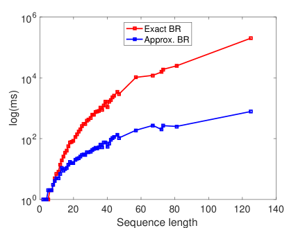
Figure 3: Comparison of double oracle performance using exact best response (LCFM Algorithm 2) and the alternative approximation method on different lengths of the sequence.

5 CONCLUSION & FUTURE WORK

This paper generalized adversarial prediction methods to structured prediction tasks with multivariate performance measures. We investigated the benefits of this approach by addressing two key NLP tasks: word alignment evaluated using the alignment error rate and named entity recognition using chain structures evaluated using the F-score. The algorithms for finding the best response for each task are described in detail. In our future work, we plan to further extend adversarial prediction to other tasks of interest in NLP and computer vision. Also, we plan to further study and characterize the multivariate performance measures that can be efficiently optimized within the adversarial prediction framework, and explore the effectiveness of approximation during constraint generation.

References

- Berkelaar et al. (2004) M. Berkelaar, K. Eikland, P. Notebaert, et al. lpsolve: Open source (mixed-integer) linear programming system. Eindhoven U. of Technology, 2004.
- Cherry and Lin (2006) C. Cherry and D. Lin. Soft syntactic constraints for word alignment through discriminative training. In Proceedings of the COLING/ACL on Main conference poster sessions, pages 105–112. Association for Computational Linguistics, 2006.
- Cormen et al. (2001) T. H. Cormen, C. E. Leiserson, R. L. Rivest, and C. Stein. Introduction to algorithms, volume 6. MIT press Cambridge, 2001.
- Cortes and Vapnik (1995) C. Cortes and V. Vapnik. Support vector machine. Machine learning, 20(3):273–297, 1995.
- Dembczynski et al. (2011) K. J. Dembczynski, W. Waegeman, W. Cheng, and E. Hüllermeier. An exact algorithm for F-measure maximization. In Advances in Neural Information Processing Systems, pages 1404–1412, 2011.
- Durrett and Klein (2015) G. Durrett and D. Klein. Neural crf parsing. In Proceedings of the 53rd Annual Meeting of the Association for Computational Linguistics and the 7th International Joint Conference on Natural Language Processing (Volume 1: Long Papers), pages 302–312, 2015.
- Dyer et al. (2013) C. Dyer, V. Chahuneau, and N. A. Smith. A simple, fast, and effective reparameterization of ibm model 2. Association for Computational Linguistics, 2013.
- Ferguson (2014) T. S. Ferguson. Game theory, second edition. 2014. URL https://www.math.ucla.edu/~tom/Game_Theory/Contents.html.
- Finkel et al. (2005) J. R. Finkel, T. Grenager, and C. Manning. Incorporating non-local information into information extraction systems by gibbs sampling. In Proceedings of the 43rd Annual Meeting on Association for Computational Linguistics, pages 363–370. Association for Computational Linguistics, 2005.
- Finkel et al. (2008) J. R. Finkel, A. Kleeman, and C. D. Manning. Efficient, feature-based, conditional random field parsing. In ACL, volume 46, pages 959–967, 2008.
- Haghighi et al. (2009) A. Haghighi, J. Blitzer, J. DeNero, and D. Klein. Better word alignments with supervised itg models. In Proceedings of the Joint Conference of the 47th Annual Meeting of the ACL and the 4th International Joint Conference on Natural Language Processing of the AFNLP: Volume 2-Volume 2, pages 923–931. Association for Computational Linguistics, 2009.
- Hoffgen et al. (1995) K.-U. Hoffgen, H.-U. Simon, and K. S. Vanhorn. Robust trainability of single neurons. Journal of Computer and System Sciences, 50(1):114–125, 1995.
- Jurafsky and Martin (2008) D. Jurafsky and J. H. Martin. Speech and Language Processing: An Introduction to Natural Language Processing, Computational Linguistics, and Speech Recognition. Prentice Hall PTR, 2 edition, 2008.
- Kim et al. (2003) T. Kim, S. E. F, and F. De Meulder. Introduction to the conll-2003 shared task: Language-independent named entity recognition. In Proceedings of the seventh conference on Natural language learning at HLT-NAACL 2003-Volume 4, pages 142–147. Association for Computational Linguistics, 2003.
- Kociskỳ et al. (2014) T. Kociskỳ, K. M. Hermann, and P. Blunsom. Learning bilingual word representations by marginalizing alignments. pages 224––229, 2014.
- Lafferty et al. (2001) J. Lafferty, A. McCallum, and F. C. Pereira. Conditional random fields: Probabilistic models for segmenting and labeling sequence data. 2001.
- Lawler (2001) E. L. Lawler. Combinatorial optimization: networks and matroids. Courier Corporation, 2001.
- Lee et al. (2013) H. Lee, A. Chang, Y. Peirsman, N. Chambers, M. Surdeanu, and D. Jurafsky. Deterministic coreference resolution based on entity-centric, precision-ranked rules. Computational Linguistics, 39(4):885–916, 2013.
- Li et al. (2016) J. Li, K. Asif, H. Wang, B. D. Ziebart, and T. Berger-Wolf. Adversarial sequence tagging. In International Joint Conference on Artificial Intelligence, 2016.
- Liu (2007) Y. Liu. Fisher consistency of multicategory support vector machines. In International Conference on Artificial Intelligence and Statistics, pages 291–298, 2007.
- Manning and Schütze (1999) C. D. Manning and H. Schütze. Foundations of statistical natural language processing, volume 999. MIT Press, 1999.
- McMahan et al. (2003) H. B. McMahan, G. J. Gordon, and A. Blum. Planning in the presence of cost functions controlled by an adversary. In Proceedings of the International Conference on Machine Learning, pages 536–543, 2003.
- Mihalcea and Pedersen (2003) R. Mihalcea and T. Pedersen. An evaluation exercise for word alignment. In Proceedings of the HLT-NAACL 2003 Workshop on Building and using parallel texts: data driven machine translation and beyond-Volume 3, pages 1–10. Association for Computational Linguistics, 2003.
- Och and Ney (2000) F. J. Och and H. Ney. Improved statistical alignment models. In Proceedings of the 38th Annual Meeting on Association for Computational Linguistics, pages 440–447. Association for Computational Linguistics, 2000.
- Och and Ney (2003) F. J. Och and H. Ney. A systematic comparison of various statistical alignment models. Computational linguistics, 29(1):19–51, 2003.
- Optimization (2014) G. Optimization. Gurobi optimizer reference manual version 5.6, 2014.
- Parambath et al. (2014) S. A. P. Parambath, N. Usunier, and Y. Grandvalet. Optimizing f-measures by cost-sensitive classification. In Proceedings of the 27th International Conference on Neural Information Processing Systems, NIPS’14, pages 2123–2131, 2014.
- Raghunathan et al. (2010) K. Raghunathan, H. Lee, S. Rangarajan, N. Chambers, M. Surdeanu, D. Jurafsky, and C. Manning. A multi-pass sieve for coreference resolution. In Proceedings of the 2010 Conference on Empirical Methods in Natural Language Processing, pages 492–501. Association for Computational Linguistics, 2010.
- Taskar et al. (2004) B. Taskar, C. Guestrin, and D. Koller. Max-margin markov networks. Advances in neural information processing systems, 16:25, 2004.
- Taskar et al. (2005a) B. Taskar, V. Chatalbashev, D. Koller, and C. Guestrin. Learning structured prediction models: A large margin approach. In Proceedings of the 22nd international conference on Machine learning, pages 896–903. ACM, 2005a.
- Taskar et al. (2005b) B. Taskar, S. Lacoste-Julien, and M. Jordan. Structured prediction via the extragradient method. In NIPS, pages 1345–1352, 2005b.
- Taskar et al. (2005c) B. Taskar, S. Lacoste-Julien, and D. Klein. A discriminative matching approach to word alignment. In Proceedings of the conference on Human Language Technology and Empirical Methods in Natural Language Processing, pages 73–80. Association for Computational Linguistics, 2005c.
- Tsochantaridis et al. (2004) I. Tsochantaridis, T. Hofmann, T. Joachims, and Y. Altun. Support vector machine learning for interdependent and structured output spaces. In Proceedings of the International Conference on Machine Learning, page 104. ACM, 2004.
- von Neumann and Morgenstern (1947) J. von Neumann and O. Morgenstern. Theory of Games and Economic Behavior. Princeton University Press, 1947.
- Wang et al. (2015) H. Wang, W. Xing, K. Asif, and B. Ziebart. Adversarial prediction games for multivariate losses. In Advances in Neural Information Processing Systems, pages 2710–2718, 2015.
- Wang et al. (2013) M. Wang, W. Che, and C. D. Manning. Joint word alignment and bilingual named entity recognition using dual decomposition. In ACL (1), pages 1073–1082, 2013.