Intelligent Power Control for Spectrum Sharing in Cognitive Radios: A Deep Reinforcement Learning Approach

Abstract

We consider the problem of spectrum sharing in a cognitive radio system consisting of a primary user and a secondary user. The primary user and the secondary user work in a non-cooperative manner. Specifically, the primary user is assumed to update its transmit power based on a pre-defined power control policy. The secondary user does not have any knowledge about the primary user’s transmit power, or its power control strategy. The objective of this paper is to develop a learning-based power control method for the secondary user in order to share the common spectrum with the primary user. To assist the secondary user, a set of sensor nodes are spatially deployed to collect the received signal strength information at different locations in the wireless environment. We develop a deep reinforcement learning-based method, which the secondary user can use to intelligently adjust its transmit power such that after a few rounds of interaction with the primary user, both users can transmit their own data successfully with required qualities of service. Our experimental results show that the secondary user can interact with the primary user efficiently to reach a goal state (defined as a state in which both users can successfully transmit their data) from any initial states within a few number of steps.

I Introduction

The dramatically increasing demand for spectrum resources requires new intelligent methods to enhance the spectrum efficiency. Per the Federal Communications Commission (FCC) [1], the spectrum in general is severely underutilized with the utilization rate of some bands as low as $15\%$. In order to improve the spectrum efficiency, the notion of spectrum sharing with secondary users through cognitive radios is highly motivated [2]. Specifically, users from a secondary network are allowed to access the spectrum owned by licensed users (also called primary users) without causing harmful interference.

According to the roles of the primary user, the operation of spectrum sharing or dynamic spectrum access can be classified into a passive primary user model and an active primary user model [3]. In many spectrum sharing studies, e.g. [4, 5, 6, 7], it is assumed that the operations of secondary users are transparent to the primary user so that the primary user does not need to adapt its transmission parameters. The transparency of secondary to primary can be accomplished by letting the secondary user to perform spectrum sensing to explore idle spectrum [4] or to strictly control its transmit power such that the interference to the primary networks is under a desired threshold [5, 6, 7]. However, some works in literature, e.g. [3, 8, 9, 10], also considered an active model in which some (cooperative or non-cooperative) interaction between the primary user and the secondary user are allowed to obtain improved transmission performance or economic compensations. For example, in [3], the spectrum sharing task is formulated as a Nash bargaining game which requires interaction between the primary user and the secondary user to reach a desired equilibrium. Also, in [10], to achieve spectrum sharing, the primary user and the secondary user are allowed to interact with each other to update their respective transmit powers. For the active model, a dynamic power control strategy is necessary for all users in the network such that a minimum quality of service (QoS) for successful data transmission is satisfied for both the primary and the secondary users.

Most existing works address this dynamic power control problem from an optimization perspective. In [11], a distributed constrained power control (DCPC) algorithm was proposed. Given the signal-to-interference-plus-noise ratio (SINR) and the required SINR threshold, the DCPC algorithm iteratively adjusts the transmit power of each transmitter such that all receivers are provided with their desired QoS requirements. Based on [11], modified approaches with different constraints or scenarios were developed [12, 13, 14, 10, 15, 16]. Other optimization-based methods were also proposed [17, 18, 19] in recent years. Besides optimization-based methods, power allocation from the game theory’s point of view was also studied [20, 21, 22, 23]. In [21], the power allocation problem was formulated as a noncooperative game with selfish users, where a sufficient condition for the existence of a Nash equilibrium was provided, and a stochastic power adaption with conjecture-based multiagent Q-learning approach was developed. However, the proposed approach requires that each user has the knowledge of the channel state information of every transmitter-receiver pair in the network, which may be infeasible in practice.

Reinforcement learning [24], also known as Q-learning, has been explored for cognitive radio applications such as dynamic spectrum access [25, 26, 27, 28, 29, 30, 31]. Using the experience and reward from the environment, users iteratively optimize their strategy to achieve their goals. Recently, deep reinforcement learning was introduced and proves its competence for challenging tasks, say Go and Atari games [32, 33, 34]. Unlike conventional reinforcement learning which is limited to domains with handcrafted features or low-dimensional observations, agents trained with deep reinforcement learning are able to learn their action-value policies directly from high-dimensional raw data such as images or videos [34]. Also, as to be shown by our experimental results, deep reinforcement learning can help learn an effective action-value policy even when the state observations are corrupted by random noise or measurement errors, while the conventional Q-learning approach is impractical for such problems due to the infinite number of states in the presence of random noise. This characteristic makes deep reinforcement learning suitable for wireless communication applications whose state measurements are generally random in nature.

In this paper, we consider a simple cognitive radio scenario consisting of a primary user and a secondary user. The primary user and the secondary user work in a non-cooperative manner, where the primary user adjusts its transmit power based on its own pre-defined power control policy. The objective is to let the secondary user learn an intelligent power control policy through its interaction with the primary user. We assume that the secondary user does not have any knowledge about the primary user’s transmit power, as well as its power control strategy. To assist the secondary user, a number of sensors are spatially deployed to collect the received signal strength (RSS) information at different locations in the wireless environment. We develop an intelligent power control policy for the secondary user by resorting to the deep reinforcement learning approach. Specifically, the use of deep reinforcement learning, instead of the conventional reinforcement learning, is to overcome the difficulty caused by random variations in the RSS measurements. Our experimental results show that, with the aid of the learned power control policy, the secondary user can intelligently adjust its transmit power such that a goal state can be reached from any initial state within a few number of transition steps.

The rest of the paper is organized as follows. Table I specifies the frequently-used symbols in this paper. The system model and the problem formulation are discussed in Section II. In Section III, we develop a deep reinforcement learning algorithm for power control for the secondary user. Experimental results are provided in Section IV, followed by concluding remarks in Section V.

TABLE I: Table of Symbols

$p_{1}$	transmit power of primary user
$p_{2}$	transmit power of secondary user
$h_{ij}$	channel gain from transmitter $\text{Tx}_{i}$ to receiver $\text{Rx}_{j}$
$N_{i}$	noise power of receiver $\text{Rx}_{i}$
$\text{SINR}_{i}$	signal to interference plus noise ratio at receiver $\text{Rx}_{i}$
$\eta_{i}$	minimum SINR requirement for receiver $\text{Rx}_{i}$
$N$	number of sensor nodes
$S_{n}$	sensor node $n$
$P_{n}^{r}$	receive power at sensor node $n$
$g_{in}$	path loss between transmitter $\text{Tx}_{i}$ and sensor $n$
$\sigma_{n}^{2}$	variance of the Gaussian random variable $w_{n}$
$\boldsymbol{s}$	state of the Markov decision process
$a$	action of the Markov decision process
$r$	reward of the Markov decision process

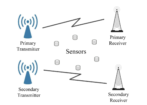
Figure 1: A schematic for spectrum sharing in cognitive radio networks.

II System Model

Consider a cognitive radio network consisting of a primary user and a secondary user, where the secondary user aims to share a common spectrum resource with the primary user, without causing harmful interference to the primary user. The primary user consists of a primary transmitter ($\text{Tx}_{1}$) and a primary receiver ($\text{Rx}_{1}$), and the secondary user consists of a secondary transmitter ($\text{Tx}_{2}$) and a secondary receiver ($\text{Rx}_{2}$), see Fig. 1. In our setup, we assume that the primary user and the secondary user are working in a non-cooperative way, in which the primary user is unaware of the existence of the secondary user, and adjusts its transmit power based on its own power control policy. Nevertheless, it should be noted that since the power control policy for the primary user is dependent on the environment (cf. (2) and (4)), the action taken by the secondary user at the current time will affect the primary user’s next move in an implicit way. There is also no communication between the primary network and the secondary network. Thus the secondary user has no knowledge about the primary user’s transmit power and its power control policy. For simplicity, we, at this point, assume that the primary user and the secondary user synchronously update their respective transmit power and the transmit power is adjusted on a time framed basis. We will show later our proposed scheme also works when the synchronous assumption does not hold.

The objective here is to help the secondary user learn an efficient power control policy such that, after a few rounds of power adjustment, both the primary user and the secondary user are able to transmit their data successfully with required QoSs. Clearly, this task cannot be accomplished if the secondary user only knows its own transmit power. To assist the secondary user, a set of sensor nodes are employed to measure the received signal strength (RSS) at different locations in the wireless environment. The RSS measurements are related to both users’ transmit power, thus revealing the state information of the system. We assume that the RSS information is accessible to the secondary user. Note that collecting the RSS information from spatially distributed sensor nodes is a basic requirement for many applications, e.g. source localization [35]. For our problem, each node only needs to report the RSS information once per time frame, which involves a low data rate. Therefore some conventional technologies such as the Zigbee [36] which delivers low-latency communication for wireless mesh networks can be employed to provide timely feedback of the RSS information from sensor nodes to the secondary user.

For both the primary user and the secondary user, the QoS is measured in terms of the SINR. Let $p_{1}$ and $p_{2}$ denote the transmit power of the primary user and the secondary user, respectively. The SINR for the $i$th receiver is given as

$$\text{SINR}_{i}=\frac{|h_{ii}|^{2}p_{i}}{\sum_{j\neq i}|h_{ji}|^{2}p_{j}+N_{i}}\quad i=1,2$$ (1)

where $h_{ij}$ denotes the channel gain from the transmitter $\text{Tx}_{i}$ to the receiver $\text{Rx}_{j}$, and $N_{i}$ is the noise power at the receiver $\text{Rx}_{i}$. We assume that the primary receiver and the secondary receiver have to satisfy a minimum SINR requirement for successful reception, i.e. $\text{SINR}_{i}\geq\eta_{i},i=1,2$.

To meet the QoS requirement, the primary user is supposed to adaptively adjust its transmit power based on its own power control policy. In this paper, two different power control strategies are considered for the primary user. Note that our proposed method also works if the primary user adopts other power control policies. For the first strategy, the transmit power of the primary user is updated according to the classical power control algorithm [11]

$$p_{1}(k+1)=D\left(\frac{\eta_{1}p_{1}(k)}{\text{SINR}_{1}(k)}\right)$$ (2)

where $\text{SINR}_{1}(k)$ denotes the SINR measured at the primary receiver at the $k$th time frame, $p_{1}(k)$ denotes the transmit power at the $k$th time frame, here we assume that the transmit power is adjusted on a time framed basis. $D(\cdot)$ is a discretization operation which maps continuous-valued levels into a set of discrete values

$$\mathcal{P}_{1}\triangleq\{p^{p}_{1},\ldots,p^{p}_{L_{1}}\}$$ (3)

where $p^{p}_{1}\leq\ldots\leq p^{p}_{L_{1}}$. More precisely, we let $D(x)$ equal the nearest discrete level that is no less than $x$ and let $D(x)=p_{L_{1}}^{p}$ if $x>p_{L_{1}}^{p}$. For the second power control strategy, suppose the transmit power at the $k$th time frame is $p_{1}(k)=p_{j}^{p}$, where $p_{j}^{p}\in\mathcal{P}_{1}$. The transmit power of the primary user is updated according to

$$p_{1}(k+1)=\begin{cases}p_{j+1}^{p}&\text{if}\ p_{j}^{p}\leq\tau\leq p_{j+1}^{p}\ \text{and}\ j+1\leq L_{1}\\ p_{j-1}^{p}&\text{if}\ \tau\leq p_{j-1}^{p}\ \text{and}\ j-1\geq 1\\ p_{j}^{p}&\text{otherwise}\end{cases}$$ (4)

where $\tau\triangleq\eta_{1}p_{1}(k)/\text{SINR}_{1}(k)$. We see that compared to (2), the power control policy (4) has a more conservative behavior: it updates its transmit power in a stepwise manner. Specifically, it increases its power (by one step) when $\text{SINR}_{1}(k)\leq\eta_{1}$ and $\hat{\eta}\geq\eta_{1}$, and decreases its power (by one step) when $\text{SINR}_{1}(k)\geq\eta_{1}$ and $\hat{\eta}\geq\eta_{1}$; otherwise it will stay on the current power level. Here $\hat{\eta}\triangleq\text{SINR}_{1}(k)p_{1}(k+1)/p_{1}(k)$ is the ‘predicted’ SINR at the $(k+1)$th time frame.

Suppose $N$ sensors are deployed to spatially sample the RSS information. Let $S_{n}$ denote node $n$, and $P_{n}^{r}(k)$ denote the receive power at sensor $n$ at the $k$th frame. In our paper, the following model is used to simulate the state (i.e. RSS) observations

$$P_{n}^{r}(k)=p_{1}(k)g_{1n}+p_{2}(k)g_{2n}+w_{n}(k)$$ (5)

where $p_{1}(k)$ and $p_{2}(k)$ represent the transmit power of the primary user and the secondary user, respectively, $g_{1n}$ denotes the path loss between the primary transmitter and sensor $n$, $g_{2n}$ denotes the path loss between the secondary transmitter and sensor $n$, and $w_{n}(k)$, a zero mean Gaussian random variable with variance $\sigma_{n}^{2}$, is used to account for the random variation caused by shadowing effect and estimation errors. For free-space propagation, according to the Friis law [37], $g_{1n}$ and $g_{2n}$ are respectively given by

$$g_{1n}=\left(\frac{\lambda}{4\pi d_{1n}}\right)^{2}\quad g_{2n}=\left(\frac{\lambda}{4\pi d_{2n}}\right)^{2}$$ (6)

where $\lambda$ is the signal wavelength, $d_{1n}$ ($d_{2n}$) denotes the distance between the primary (secondary) transmitter and node $n$.

We also assume that the transmit power of the secondary user is chosen from a finite set

$$\mathcal{P}_{2}\triangleq\{p^{s}_{1},\ldots,p^{s}_{L_{2}}\}$$ (7)

where $p^{s}_{1}\leq\ldots\leq p^{s}_{L_{2}}$. The objective of the secondary user is to learn how to adjust its transmit power based on the collected RSS information $\{P_{n}^{r}(k)\}_{n}$ at each time frame such that after a few rounds of power adjustment, both the primary user and the secondary user can meet their respective QoS requirements for successful data transmissions. Note that we suppose there exists at least a pair of transmit power $\{p^{p}_{l_{1}},p^{s}_{l_{2}}\}$ such that the primary receiver and the secondary receiver satisfy their respective QoS (SINR) requirements, i.e. $\text{SINR}_{i}\geq\eta_{i},i=1,2$.

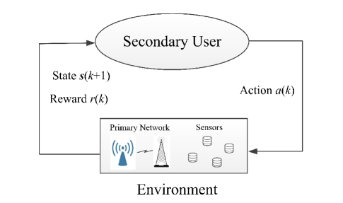
Figure 2: Interaction between the secondary user and the environment (i.e. the primary user).

III A Deep Reinforcement Learning Approach for Power Control

We see that the secondary user, at each time frame, has to take an action (i.e. choose a transmit power from a pre-specified power set $\mathcal{P}_{2}$) based on its current state

$$\boldsymbol{s}(k)\triangleq\left[P_{1}^{r}(k)\phantom{0}\ldots\phantom{0}P_{N}^{r}(k)\right]^{T}$$ (8)

This power control process is essentially a Markov decision process (MDP) because after the decision maker (i.e. the secondary user) chooses any action $a(k)=p_{2}(k+1)$ in state $\boldsymbol{s}(k)$, the process will move into a new state $\boldsymbol{s}(k+1)$ which depends on the current state $\boldsymbol{s}(k)$ and the decision maker’s action $a(k)$, and given $\boldsymbol{s}(k)$ and $a(k)$, the next state is conditionally independent of all previous states and actions. Also, after moving into a new state, the decision maker will receive a corresponding reward $r(k)\triangleq r(\boldsymbol{s}(k),a(k))$ which can be defined as

$$r(k)\triangleq\begin{cases}10&\text{if}\ \text{SINR}_{1}(k+1)\geq\eta_{1}\ \text{and}\ \text{SINR}_{2}(k+1)\geq\eta_{2}\\ 0&\text{otherwise}\end{cases}$$

The interaction between the secondary user and the environment is shown in Fig. 2. Note that here the decision maker (secondary user) is assumed to know whether the transmission between the primary transmitter and the primary receiver is successful or not. In practice, such knowledge may be obtained by monitoring an acknowledgment signal sent by the primary receiver to indicate successful receipt of a transmission from the primary transmitter.

The core problem of MDPs is to learn a “policy” for the decision maker: a function $\pi$ that specifies the action $\pi(\boldsymbol{s})$ that the decision maker will choose when in state $\boldsymbol{s}$. More precisely, the goal of the secondary user is to learn a policy $\pi$ for selecting its action $a(k)$ based on the current state $\boldsymbol{s}(k)$ in a way that maximizes a discounted cumulative reward which is defined as [24]

$$V^{\pi}\left(\boldsymbol{s}(k)\right) \triangleq\sum_{i=k}^{T^{\prime}}\gamma^{i-k}r(i)$$ (9)

where $\gamma$ is the discount factor and $T^{\prime}$ denotes the time frame at which the goal state is reached. For our problem, the goal state is defined as a state in which $\text{SINR}_{i}(k)\geq\eta_{i},i=1,2$. Thus, the task becomes learning an optimal policy $\pi^{*}$ that maximizes $V^{\pi}$, i.e.

$$\pi^{*} =\mathop{\arg\max}_{\pi}{V^{\pi}(\boldsymbol{s})}\quad\forall\boldsymbol{s}$$ (10)

Directly learning $\pi^{*}$ is difficult. In reinforcement learning, Q-learning provides an alternative approach to solve (10) [38]. Instead of learning $\pi^{*}$, an action-value (also known as Q) function is introduced to evaluate the expected discounted cumulative reward after taking some action $\boldsymbol{a}$ in a given state $\boldsymbol{s}$. When such an action-value function is learned, the optimal policy can be constructed by simply selecting the action with the highest value in each state. The basic idea behind the Q-learning and many other reinforcement learning algorithms is to iteratively update the action-value function according to a simple value iteration update rule

$$Q(\boldsymbol{s},a)=r(\boldsymbol{s},a)+\gamma\max_{a^{\prime}}{Q(\boldsymbol{s}^{\prime},a^{\prime})}$$ (11)

The above update rule is also known as the Bellman equation [39], in which $\boldsymbol{s}^{\prime}$ is the state resulting from applying action $a$ to the current state $\boldsymbol{s}$. It has been proved that the value iteration algorithm (11) converges to the optimal action-value function, which is defined as the maximum expected discounted cumulative reward by following any policy, after taking some action $\boldsymbol{a}$ in a given state $\boldsymbol{s}$. For the Q-learning, the number of states is finite and the action-value function is estimated separately for each state, thus leading to a Q-table or a Q-matrix, with its rows representing the states and its columns representing the possible actions. After the Q-table converges, one can select an action $a$ which has the largest value of $Q(\boldsymbol{s},a)$ as the optimal action in state $\boldsymbol{s}$.

Unfortunately, due to the random variation in the RSS measurement, the value of $\boldsymbol{s}$ is continuous. As a result, the Q-learning approach is impractical for our problem since we could have an infinite number of states. To overcome this issue, we resort to the deep Q-network (DQN) proposed in [33]. Unlike the conventional Q-learning method that generates a finite action-value table, for the DQN, the table is replaced by a deep neural network $Q(\boldsymbol{s},a;\boldsymbol{\theta})$ to approximate the action-value function, where $\boldsymbol{\theta}$ denotes the weights of the Q-network. Specifically, given an input $\boldsymbol{s}$, the deep neural network yields an $L_{2}$-dimensional vector, with its $i$th entry representing the estimated value for choosing the action $a=p^{s}_{i}$ from $\mathcal{P}_{2}$.

The training data used to train the Q-network are generated as follows. Given $\boldsymbol{s}(k)$, at iteration $k$, we either explore a randomly selected action with probability $\varepsilon_{k}$, or select an action $a(k)$ which has the largest output $Q(\boldsymbol{s}(k),a(k);\boldsymbol{\theta}_{0})$, where $\boldsymbol{\theta}_{0}$ denotes the parameters for the current iteration. After taking the action $a(k)$, the secondary user receives a reward $r(k)$ and observes a new state $\boldsymbol{s}(k+1)$. This transition $d(k)\triangleq\{\boldsymbol{s}(k),a(k),r(k),\boldsymbol{s}(k+1)\}$ is stored in the replay memory $D$. The training of the Q-network begins when $D$ has collected a sufficient number of transitions, say $O=300$ transitions. Specifically, we randomly select a minibatch of transitions $\{d(i)|i\in\Omega_{k}\}$ from $D$, and the Q-network can be trained by adjusting the parameters $\boldsymbol{\theta}$ such that the following loss function is minimized

$$L(\boldsymbol{\theta})\triangleq\frac{1}{|\Omega_{k}|}\sum_{i\in\Omega_{k}}\left(Q^{\prime}(i)-Q(\boldsymbol{s}(i),a(i);\boldsymbol{\theta})\right)^{2}$$ (12)

in which $\Omega_{k}$ is the index set of the random minibatch used at the $k$th iteration, and $Q^{\prime}(i)$ is a value estimated via the Bellman equation by using parameters from the current iteration, i.e.

$$Q^{\prime}(i)=r(i)+\gamma\max_{a^{\prime}}Q(\boldsymbol{s}(i+1),a^{\prime};\boldsymbol{\theta}_{0})\quad\forall i\in\Omega_{k}$$ (13)

Note that unlike traditional supervised learning, the targets for DQN learning is updated as the weights $\boldsymbol{\theta}$ are refined. For clarity, we summarize our proposed DQN training algorithm in Algorithm 1.

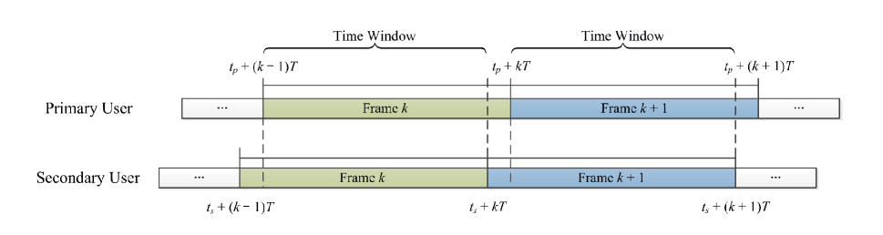
Figure 3: Asynchronous update of the transmit power for the primary user and the secondary user.

Algorithm 1 DQN Training for Power Control

   Initialize replay memory $D$ with buffer capacity $O$Initialize network $Q(\boldsymbol{s},a,\boldsymbol{\theta})$ with random weights $\boldsymbol{\theta}=\boldsymbol{\theta}_{0}$Initialize $p_{1}(1)$ and $p_{2}(1)$, then obtain $\boldsymbol{s}(1)$

  for $k=1,K$ do

     Update $p_{1}(k+1)$ via the primary user’s power control strategy (2) or (4)

     With probability $\varepsilon_{k}$ select a random action $a(k)$, otherwise select $a(k)=\max_{a}Q(\boldsymbol{s}(k),a;\boldsymbol{\theta}_{0})$

     Obtain $\boldsymbol{s}(k+1)$ via the random observation model (5) and observe reward $r(k)$

     Store transition $d(k)\triangleq\{\boldsymbol{s}(k),a(k),r(k),\boldsymbol{s}(k+1)\}$ in $D$

     if $k\geq O$ then

        Sample a random minibatch of transitions $\{d(i)|i\in\Omega_{k}\}$ from $D$, where the indexes in $\Omega_{k}$ are uniformly chosen at random

        Update $\boldsymbol{\theta}$ by minimizing the loss function (12), where targets $Q^{\prime}(i)$ are given by (13)

        Set $\boldsymbol{\theta}_{0}=\mathop{\arg\min}_{\boldsymbol{\theta}}L(\boldsymbol{\theta})$

     end if

     if $\boldsymbol{s}(k)$ is a goal state then

        Initialize $p_{1}(k+1)$ and $p_{2}(k+1)$, then obtain $\boldsymbol{s}(k+1)$

     end if

  end for

After training, the secondary user can choose the action which yields the largest estimated value $Q(\boldsymbol{s},a,\boldsymbol{\theta}^{*})$. For clarity, the proposed DQN-based power control scheme for the secondary user is summarized in Algorithm 2. We would like to point out that during the DQN training process, the secondary user requires the knowledge of whether the QoS requirements for the primary user and the secondary user are satisfied. Nevertheless, after the DQN is trained, the secondary user only needs the feedback from sensors to decide its next transmit power.

We discuss the convergence issue of the proposed power control policy. Suppose $\boldsymbol{s}$ is a goal state. If the transmit power of the secondary user remains unchanged, then it is easy to show that the next state $\boldsymbol{s}^{\prime}$ is also a goal state, whichever of (2) and (4) is chosen for the primary user to update its transmit power. On the other hand, the secondary user will eventually learn to choose a transmit power such that the next state $\boldsymbol{s}^{\prime}$ remains a goal state. Therefore we can conclude that once $\boldsymbol{s}$ reaches a goal state, it will stay at the goal state until the data transmission is over. Suppose the goal state is lost due to the discontinuity of data transmission, and the secondary user wants to restart a new transmission. In this case, learning is no longer required. The secondary user can select its transmit power according to the learned power control policy.

In our previous discussion, we assume that the primary user and the secondary user synchronously update their respective transmit power. Nevertheless, we would like to point out that the synchronous assumption is not necessarily required by our proposed scheme. Suppose the time frames between the primary user and the secondary user are not strictly synchronized (see Fig. 3). Both the primary user and the secondary user update their transmit power at the beginning of their respective time frames, that is, the primary user adjusts its transmit power at time $t_{p},t_{p}+T,t_{p}+2T,\ldots$, and the secondary user updates its transmit power at time $t_{s},t_{s}+T,t_{s}+2T,\ldots$, where $T$ denotes the duration of each frame. Without loss of generality, we assume $T>t_{p}-t_{s}>0$. Clearly, our intelligent power control scheme would function the same as in the synchronous case if both the primary user and the secondary user perform their respective tasks, i.e. gather necessary information (i.e. $\text{SINR}_{1}(k)$ for the primary user, $\text{SINR}_{1}(k)$, $\text{SINR}_{2}(k)$, and $\boldsymbol{s}(k)$ for the secondary user) and make decisions during the time window $[t_{p}+(k-1)T,t_{s}+kT]$.

Algorithm 2 DQN-based Power Control Strategy

   Initialize $p_{2}(1)$, then obtain $\boldsymbol{s}(1)$

  for $k=1,K$ do

     Select $a(k)=\max_{a}Q(\boldsymbol{s}(k),a;\boldsymbol{\theta}^{*})$

     Obtain $\boldsymbol{s}(k+1)$

  end for

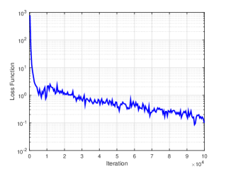
(a) Loss function vs. the number of iterations.

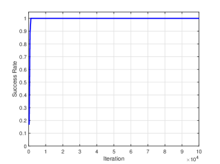
(b) Success rate vs. the number of iterations.

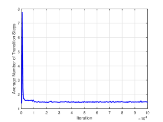
(c) Average number of transition steps vs. the number of iterations.

Figure 4: Loss function, success rate, and average number of transition steps vs. the number of iterations $k$ used for training, where $N=10$, $\sigma_{n}=(p_{1}^{p}g_{1n}+p_{1}^{s}g_{2n})/10$.

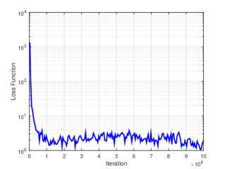
(a) Loss function vs. the number of iterations.

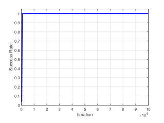
(b) Success rate vs. the number of iterations.

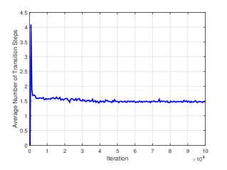
(c) Average number of transition steps vs. the number of iterations.

Figure 5: Loss function, success rate, and average number of transition steps vs. the number of iterations $k$ used for training, where $N=10$, $\sigma_{n}=(p_{1}^{p}g_{1n}+p_{1}^{s}g_{2n})/3$.

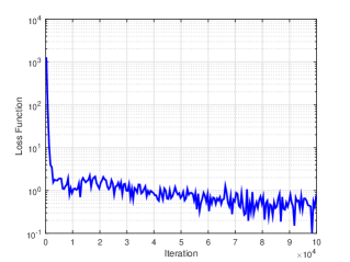
(a) Loss function vs. the number of iterations.

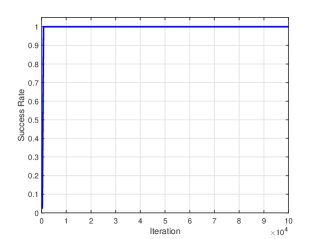
(b) Success rate vs. the number of iterations.

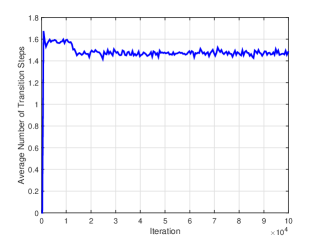
(c) Average number of transition steps vs. the number of iterations.

Figure 6: Loss function, success rate, and average number of transition steps vs. the number of iterations $k$ used for training, where $N=3$, $\sigma_{n}=(p_{1}^{p}g_{1n}+p_{1}^{s}g_{2n})/10$.

IV Experimental Results

We now carry out experiments to illustrate the performance of our proposed DQN-based power control algorithm. In our experiments, the transmit power (in Watt) of both the primary user and the secondary user is chosen from a pre-defined set $\mathcal{P}_{1}=\mathcal{P}_{2}=\{0.05,0.1,\ldots,0.4\}$, and the noise power at $\text{Rx}_{1}$ and $\text{Rx}_{2}$ is set to $N_{1}=N_{2}=0.01$W. For simplicity, the channel gains from the primary/secondary transmitter to the primary/secondary receivers are assumed to be $h_{ij}=1,\forall i,j$. The minimum SINR requirements for successful reception for the primary user and the secondary user are set to $\eta_{1}=1.2$, $\eta_{2}=0.7$, respectively. It can be easily checked that there exists a pair of transmit power $\{p_{1},p_{2}\}$ which ensures that the QoSs of the primary user and the secondary user are satisfied. Also, a total number of $N$ sensors are employed to collect the RSS information to assist the secondary user to learn a power control policy. The distance $d_{ij}$ between the transmitter $\text{Tx}_{i}$ and the sensor node $S_{j}$ is uniformly distributed in the interval $[100,300]$ (in meters).

(a) Loss function vs. the number of iterations.

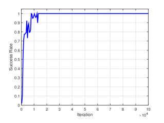
(b) Success rate vs. the number of iterations.

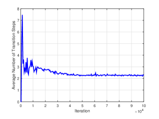
(c) Average number of transition steps vs. the number of iterations.

Figure 7: Loss function, success rate, and average number of transition steps vs. the number of iterations $k$ used for training, where $N=10$, $\sigma_{n}=(p_{1}^{p}g_{1n}+p_{1}^{s}g_{2n})/10$.

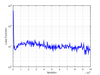
(a) Loss function vs. the number of iterations.

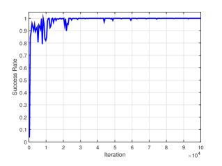
(b) Success rates vs. the number of iterations.

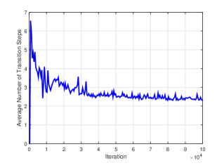
(c) Average number of transition steps vs. the number of iterations.

Figure 8: Loss function, success rate, and average number of transition steps vs. the number of iterations $k$ used for training, where $N=10$, $\sigma_{n}=(p_{1}^{p}g_{1n}+p_{1}^{s}g_{2n})/3$.

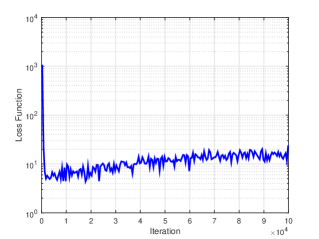
(a) Loss function vs. the number of iterations.

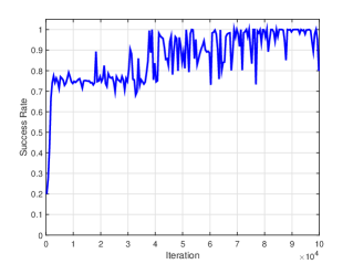
(b) Success rate vs. the number of iterations.

(c) Average number of transition steps vs. the number of iterations.

Figure 9: Loss function, success rate, and average number of transition steps vs. the number of iterations $k$ used for training, where $N=3$, $\sigma_{n}=(p_{1}^{p}g_{1n}+p_{1}^{s}g_{2n})/10$.

In our experiments, the deep neural network (DNN) used to approximate the action-value function consists of three fully-connected feedforward hidden layers, and the number of neurons in the three hidden layers are $256$, $256$, and $512$, respectively. Rectified linear units (ReLUs) are employed as the activation function for the first and the second hidden layers. A ReLU has output 0 if the input is less than 0, and raw output otherwise. For the last hidden layer, the tanh function is used as the activation function. The Adam algorithm [40] is adopted for updating the weights $\boldsymbol{\theta}$, where the size of a minibatch is set to $256$. We assume that the replay memory $D$ contains $N_{D}=400$ most recent transitions, and in each iteration, the training of $\boldsymbol{\theta}$ begins only when $D$ stores more than $O=300$ transitions. The total number of iterations is set to $K=10^{5}$. The probability of exploring new actions linearly decreases with the number of iterations from $0.8$ to $0$. Specifically, at iteration $k$, we let

$$\varepsilon_{k}=0.8(1-k/K)$$ (14)

We use Algorithm 1 to train the network, and use Algorithm 2 to check its performance.

The performance is evaluated via two metrics, namely, the success rate and the average number of transition steps. The success rate is computed as the ratio of the number of successful trials to the total number of independent runs. A trial is considered successful if $\boldsymbol{s}$ moves to a goal state within 20 time frames. The average number of transition steps is defined as the average number of time frames required to reach a goal state if a trial is successful.

We now study the performance of the deep reinforcement learning approach. Specifically, we examine the loss function, the success rate, and the average number of transition steps as a function of the number of iterations $k$ used for training. During training, the loss function is calculated according to (12). After $k$ iterations of training, the secondary user can use the trained network to interact with the primary user. The success rate and the average number of transition steps are used to evaluate how well the network is trained. Results are averaged over $10^{3}$ independent runs, in which a random initial state is selected for each run. Fig. 4 plots the loss function, the success rate, and the average number of transition steps vs. the number of iterations $k$, where we set $N=10$, the standard deviation of the random variable used to account for the shadowing effect and measurement errors is set to $\sigma_{n}=(p_{1}^{p}g_{1n}+p_{1}^{s}g_{2n})/10$, and the primary user employs (2) to update its transmit power. We see that the secondary user, after only $10^{3}$ iterations of training, can learn an efficient power control policy which ensures that a goal state can be reached quickly (with $1.5$ average number of transition steps) from any initial states with probability one. Fig. 5 and Fig. 6 depict the loss function, the success rate, and the average number of transition steps vs. $k$ for different choices of $N$ and $\sigma_{n}$, where we set $N=10$, $\sigma_{n}=(p_{1}^{p}g_{1n}+p_{1}^{s}g_{2n})/3$ for Fig. 5 and $N=3$, $\sigma_{n}=(p_{1}^{p}g_{1n}+p_{1}^{s}g_{2n})/10$ for Fig. 6. We see that the value of the loss function becomes larger when we increase the variance $\sigma_{n}$ or decrease the number of sensors. Nevertheless, the learned policy is still very efficient and effective, attaining a success rate and an average number of transition steps similar to those in Fig. 4. This result demonstrates the robustness of the deep reinforcement learning approach.

Next, we examine the performance of the DQN-based power control method when the primary user employs the second power control policy (4) to update its transmit power. Since the policy (4) is more conservative, the task of learning an optimal power control strategy is more challenging. Fig. 7 depicts the loss function, the success rate, and the average number of transition step as a function of $k$, where we set $N=10$ and $\sigma_{n}=(p_{1}^{p}g_{1n}+p_{1}^{s}g_{2n})/10$. We observe that for this example, more iterations (about $1.5\times 10^{4}$) are required for training to reach a success rate of one. Moreover, the learned policy requires an average number of transition steps of $2.5$ to reach a goal state. The increased number of transition steps is because the second policy used by the primary user only allow its transmit power to increase/decrease by a single level at each step. Thus more steps are needed to reach the goal state. Fig. 8 and Fig. 9 plot the loss function, the success rate, and the average number of transition steps vs. $k$ for different choices of $N$ and $\sigma_{n}$, where we set $N=10$, $\sigma_{n}=(p_{1}^{p}g_{1n}+p_{1}^{s}g_{2n})/3$ for Fig. 8 and $N=3$, $\sigma_{n}=(p_{1}^{p}g_{1n}+p_{1}^{s}g_{2n})/10$ for Fig. 9. For this example, we see that a large variance in the state observations and an insufficient number of sensors lead to performance degradation. In particular, the proposed method incurs a considerable performance loss when fewer sensors are deployed. This is because the random variation in the state observations makes different states less distinguishable from each other and prevents the agent from learning an effective policy, but using more sensors helps neutralize the effect of random variations.

Lastly, we compare the DQN-based power control method with the DCPC algorithm [11] which was developed for power control in an optimization framework. For the DCPC algorithm, the primary user and secondary user use the following power control policy to update their respective transmit power:

$$p_{1}(k+1)=\min\left\{p^{p}_{L_{1}},\frac{\eta_{1}p_{1}(k)}{\text{SINR}_{1}(k)}\right\}$$ (15)

$$p_{2}(k+1)=\min\left\{p^{s}_{L_{2}},\frac{\eta_{2}p_{2}(k)}{\text{SINR}_{2}(k)}\right\}$$ (16)

For the DQN-based method, the primary user uses the policy (2) to update its transmit power, the number of sensor nodes and the state observation noise variance are set to $N=10$ and $\sigma_{n}=(p_{1}^{p}g_{1n}+p_{1}^{s}g_{2n})/10$, respectively. In Fig. 10, we examine the QoSs (i.e. SINRs) of the primary and secondary users as the iterative process evolves. We see that although both schemes can converge from an initial point, our proposed DQN-based method requires only a few transition steps to reach a goal state, while the DCPC algorithm takes tens of steps to converge. We also observe that the DQN-based scheme converges to a solution that is close to the optimal solution obtained by the DCPC algorithm, which further corroborates the effectiveness of the proposed DQN-based scheme. Note that optimization-based techniques such as the DCPC algorithm require global coordination among all users in the cognitive networks so that the primary user and the secondary user can interact in a cooperative way. In contrast, for our proposed scheme, the primary user follows its own rule to react to the environment. In other words, the interaction between the primary user and the secondary user is not planned out in advance and needs to be learned in real time. Although the training of the DQN involves a high computational complexity, after the training is completed, the operation of the power control has a very low computational complexity: given an input state $\boldsymbol{s}$, the secondary user can make a decision using simple calculations.

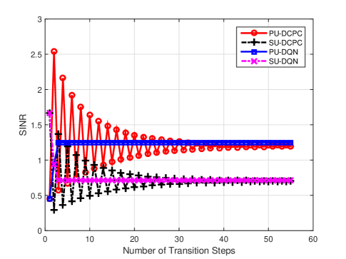
Figure 10: SINRs of the primary and secondary users vs. the number of transition steps.

V Conclusions

We studied the problem of spectrum sharing in a cognitive radio system consisting of a primary user and a secondary user. We assume that the primary user and the secondary user work in a non-cooperative way. The primary user adjusts its transmit power based on its own pre-defined power control policy. We developed a deep reinforcement learning-based method for the secondary user to learn how to adjust its transmit power such that eventually both the primary user and the secondary user are able to transmit their respective data successfully with required qualities of service. Experimental results show that the proposed learning method is robust against the random variation in the state observations, and a goal state can be reached from any initial states within only a few number of steps.

References

- [1] P. Kolodzy and I. Avoidance, “Spectrum policy task force,” Federal Commun. Commission, Washington, DC, USA, Tech. Rep. 02-135, 2002.
- [2] S. Haykin, “Cognitive radio: brain-empowered wireless communications,” IEEE Journal on Selected Areas in Communications, vol. 23, no. 2, pp. 201–220, Feb. 2005.
- [3] Y. Wu, Q. Zhu, J. Huang, and D. H. K. Tsang, “Revenue sharing based resource allocation for dynamic spectrum access networks,” IEEE J. Sel. Areas Commun., vol. 32, no. 11, pp. 2280–2296, Nov. 2014.
- [4] P. Wang, J. Fang, N. Han, and H. Li, “Multiantenna-assisted spectrum sensing for cognitive radio,” IEEE Transactions on Vehicular Technology, vol. 59, no. 4, pp. 1791–1800, May 2010.
- [5] I. Mitliagkas, N. D. Sidiropoulos, and A. Swami, “Joint power and admission control for ad-hoc and cognitive underlay networks: Convex approximation and distributed implementation,” IEEE Transactions on Wireless Communications, vol. 10, no. 12, pp. 4110–4121, December 2011.
- [6] D. I. Kim, L. B. Le, and E. Hossain, “Joint rate and power allocation for cognitive radios in dynamic spectrum access environment,” IEEE Transactions on Wireless Communications, vol. 7, no. 12, pp. 5517–5527, December 2008.
- [7] J. Tadrous, A. Sultan, and M. Nafie, “Admission and power control for spectrum sharing cognitive radio networks,” IEEE Transactions on Wireless Communications, vol. 10, no. 6, pp. 1945–1955, June 2011.
- [8] W. Su, J. D. Matyjas, and S. Batalama, “Active cooperation between primary users and cognitive radio users in heterogeneous ad-hoc networks,” IEEE Transactions on Signal Processing, vol. 60, no. 4, pp. 1796–1805, April 2012.
- [9] Q. Zhu, Y. Wu, D. H. K. Tsang, and H. Peng, “Cooperative spectrum sharing in cognitive radio networks with proactive primary system,” in 2013 IEEE/CIC International Conference on Communications in China - Workshops (CIC/ICCC), Xi’an, China, Aug,12-14 2013, pp. 82–87.
- [10] M. H. Islam, Y. C. Liang, and A. T. Hoang, “Distributed power and admission control for cognitive radio networks using antenna arrays,” in 2007 2nd IEEE International Symposium on New Frontiers in Dynamic Spectrum Access Networks, Dublin, Ireland, April,17-20 2007, pp. 250–253.
- [11] S. A. Grandhi, J. Zander, and R. Yates, “Constrained power control,” Wireless Personal Communications, vol. 1, no. 4, pp. 257–270, December 1994.
- [12] M. Xiao, N. B. Shroff, and E. K. P. Chong, “A utility-based power-control scheme in wireless cellular systems,” IEEE/ACM Transactions on Networking, vol. 11, no. 2, pp. 210–221, Apr. 2003.
- [13] T. ElBatt and A. Ephremides, “Joint scheduling and power control for wireless ad hoc networks,” IEEE Transactions on Wireless Communications, vol. 3, no. 1, pp. 74–85, Jan. 2004.
- [14] J. Tadrous, A. Sultan, M. Nafie, and A. El-Keyi, “Power control for constrained throughput maximization in spectrum shared networks,” in 2010 IEEE Global Telecommunications Conference GLOBECOM 2010, Miami, FL, USA, Dec. 6-10 2010, pp. 1–6.
- [15] Y. Xing, C. N. Mathur, M. A. Haleem, R. Chandramouli, and K. P. Subbalakshmi, “Dynamic spectrum access with QoS and interference temperature constraints,” IEEE Transactions on Mobile Computing, vol. 6, no. 4, pp. 423–433, April 2007.
- [16] S. Lee, Y. Zeng, and R. Zhang, “Retrodirective multi-user wireless power transfer with massive MIMO,” IEEE Wireless Communications Letters, vol. 7, no. 1, pp. 54–57, Feb. 2018.
- [17] Y. F. Liu, Y. H. Dai, and S. Ma, “Joint power and admission control: Non-convex approximation and an effective polynomial time deflation approach,” IEEE Transactions on Signal Processing, vol. 63, no. 14, pp. 3641–3656, July 2015.
- [18] K. Senel and S. Tekinay, “Optimal power allocation in NOMA systems with imperfect channel estimation,” in 2017 IEEE Global Communications Conference GLOBECOM 2017, Singapore, Singapore, Dec.,4-8 2017, pp. 1–7.
- [19] Y. F. Liu, M. Hong, and E. Song, “Sample approximation-based deflation approaches for chance SINR-constrained joint power and admission control,” IEEE Transactions on Wireless Communications, vol. 15, no. 7, pp. 4535–4547, July 2016.
- [20] T. Heikkinen, “A potential game approach to distributed power control and scheduling,” Computer Networks, vol. 50, no. 13, pp. 2295 – 2311, Sep. 2006.
- [21] X. Chen, Z. Zhao, and H. Zhang, “Stochastic power adaptation with multiagent reinforcement learning for cognitive wireless mesh networks,” IEEE Transactions on Mobile Computing, vol. 12, no. 11, pp. 2155–2166, Nov. 2013.
- [22] G. Yang, B. Li, X. Tan, and X. Wang, “Adaptive power control algorithm in cognitive radio based on game theory,” IET Communications, vol. 9, no. 15, pp. 1807–1811, Oct. 2015.
- [23] L. Gao, L. Duan, and J. Huang, “Two-sided matching based cooperative spectrum sharing,” IEEE Transactions on Mobile Computing, vol. 16, no. 2, pp. 538–551, Feb. 2017.
- [24] R. S. Sutton and A. G. Barto, Reinforcement learning: An introduction. Cambridge: MIT press, 1998.
- [25] M. Bennis and D. Niyato, “A Q-learning based approach to interference avoidance in self-organized femtocell networks,” in 2010 IEEE Globecom Workshops, Miami, FL, USA, Dec.,6-10 2010, pp. 706–710.
- [26] H. Li, “Multiagent Q-learning for aloha-like spectrum access in cognitive radio systems,” EURASIP Journal on Wireless Communications and Networking, vol. 2010, May 2010.
- [27] O. Naparstek and K. Cohen, “Deep multi-user reinforcement learning for dynamic spectrum access in multichannel wireless networks,” arXiv preprint arXiv:1704.02613, 2017.
- [28] F. Fu and M. van der Schaar, “Learning to compete for resources in wireless stochastic games,” IEEE Transactions on Vehicular Technology, vol. 58, no. 4, pp. 1904–1919, May 2009.
- [29] J. Lundén, V. Koivunen, S. R. Kulkarni, and H. V. Poor, “Reinforcement learning based distributed multiagent sensing policy for cognitive radio networks,” in 2011 IEEE International Symposium on Dynamic Spectrum Access Networks (DySPAN), Aachen, Germany, May,3-6 2011, pp. 642–646.
- [30] A. Alsarhan and A. Agarwal, “Spectrum sharing in multi-service cognitive network using reinforcement learning,” in 2009 First UK-India International Workshop on Cognitive Wireless Systems (UKIWCWS), New Delhi, India, Dec.,10-12 2009, pp. 1–5.
- [31] T. Wang, C. K. Wen, H. Wang, F. Gao, T. Jiang, and S. Jin, “Deep learning for wireless physical layer: Opportunities and challenges,” China Communications, vol. 14, no. 11, pp. 92–111, Nov. 2017.
- [32] V. Mnih, K. Kavukcuoglu, D. Silver, A. Graves, I. Antonoglou, D. Wierstra, and M. Riedmiller, “Playing atari with deep reinforcement learning,” arXiv preprint arXiv:1312.5602, 2013.
- [33] V. Mnih et al., “Human-level control through deep reinforcement learning,” Nature, vol. 518, pp. 529–533, Feb. 2015.
- [34] D. Silver et al., “Mastering the game of go with deep neural networks and tree search,” Nature, vol. 529, pp. 484–489, Jan. 2016.
- [35] S. Tomic, M. Beko, and R. Dinis, “RSS-based localization in wireless sensor networks using convex relaxation: Noncooperative and cooperative schemes,” IEEE Trans. Veh. Technol., vol. 64, no. 5, pp. 2037–2050, May 2015.
- [36] J. Yick, B. Mukherjee, and D. Ghosal, “Wireless sensor network survey,” Computer Networks, vol. 52, no. 12, pp. 2292–2330, Aug. 2008.
- [37] T. S. Rappaport, Wireless communications: principles and practice. NJ, USA: Prentice Hall, 2002.
- [38] C. J. C. H. Watkins and P. Dayan, “Q-learning,” Machine Learning, vol. 8, no. 3, pp. 279–292, May 1992.
- [39] R. Bellman, Dynamic programming. Princeton, NJ: Princeton University Press, 2003.
- [40] D. P. Kingma and J. Ba, “Adam: A method for stochastic optimization,” arXiv preprint arXiv:1412.6980, 2014.