Network Cache Design under Stationary Requests:
Exact Analysis and Poisson Approximation

Abstract.

The design of caching algorithms to maximize hit probability has been extensively studied. In this paper, we associate each content with a utility, which is a function of either the corresponding content hit rate or hit probability. We formulate a cache optimization problem to maximize the sum of utilities over all contents under stationary and ergodic request processes. This problem is non-convex in general but we reformulate it as a convex optimization problem when the inter-request time (irt) distribution has a non-increasing hazard rate function. We provide explicit optimal solutions for some irt distributions, and compare the solutions of the hit-rate based (HRB) and hit-probability based (HPB) problems. We formulate a reverse engineering based dual implementation of LRU under stationary arrivals. We also propose decentralized algorithms that can be implemented using limited information and use a discrete time Lyapunov technique (DTLT) to correctly characterize their stability. We find that decentralized algorithms that solve HRB are more robust than decentralized HPB algorithms. Informed by these results, we further propose lightweight Poisson approximate decentralized and online algorithms that are accurate and efficient in achieving optimal hit rates and hit probabilities.

1. Introduction

Caching plays a prominent role in networks and distributed systems for improving system performance. Since the number of contents in a system is typically significantly larger than cache capacity, the design of caching algorithms typically focuses on maximizing the number of requests that can be served from the cache. Considerable research has focused on the analysis of caching algorithms using the metric of hit probability under the Independent Reference Model (IRM) (Aven et al., 1987; Dehghan et al., 2016; Jung et al., 2003; Che et al., 2002; Panigrahy et al., 2017a; Li et al., 2018; Panigrahy et al., 2017b). However, hit rate (Fofack et al., 2012) is a more relevant performance metric in real systems. For example, pricing based on hit rate is preferable to that based on cache occupancy from the perspective of a service provider (Ma and Towsley, 2015). Furthermore, one goal of a service provider in designing hierarchical caches would be to minimize the internal bandwidth cost, which can be characterized with a utility function $U_{i}=-C_{i}(m_{i}),$ where $C_{i}(m_{i})$ is the cost associated with miss rate $m_{i}$ for content $i.$ Therefore, we focus on the hit rate.

Recently there has been a tremendous increase in the demand for different types of content with different quality of service requirements; consequently, user needs have become more heterogeneous. In order to meet such challenges, content delivery networks need to incorporate service differentiation among different classes of contents and applications. Though considerable literature has focused on the design of fair and efficient caching algorithms for content distribution, little work has focused on the provision of multiple levels of service in network and web caches.

Moreover, cache behaviors of different contents are strongly coupled by conventional caching algorithms such as LRU (Aven et al., 1987; Li et al., 2018; Garetto et al., 2016), which make it difficult for cache service providers to provide differential services. In this paper, we focus on Time-to-Live (TTL) caches. When a content is inserted into the cache due to a cache miss, a timer is set. Timer value can differ for different contents. All requests for a content before the expiration of its timer results in a cache hit, and the first request after the expiration of its timer yields a cache miss. This ability to decouple the behaviors of different contents make the TTL policy an interesting alternative to more popular algorithms like LRU. Moreover, the TTL policy has the capacity of mimicking the behaviors of many caching algorithms (Baccelli and Brémaud, 2013).

In this paper, we consider a utility-driven caching framework, where each content is associated with a utility. Content is stored and managed in the cache so as to maximize the aggregate utility for all content. A related problem has been considered in (Dehghan et al., 2016), where the authors formulated a Hit-probability Based Cache Utility Maximization (HPB-CUM) framework under IRM. The objective is to maximize the sum of utilities under a cache capacity constraint when utilities are increasing, continuously differentiable, and strictly concave function of hit probability. (Dehghan et al., 2016), (Fofack et al., 2014b) and (Panigrahy et al., 2017b) characterized optimal TTL cache policies, and also proposed distributed cache management algorithms. Here, we focus on utilities as functions of hit rates.

While characterization of hit rate under IRM is valuable, real-world request processes exhibit changes in popularity and temporal correlations in requests (Zink et al., 2008; Cha et al., 2007). To account for them, in this paper, we consider a very general traffic model where requests for distinct contents are described by mutually independent stationary and ergodic point processes (Baccelli and Brémaud, 2013).

1.1. Contributions

Our main contributions in this paper can be summarized as follows.

1) We formulate a Hit-rate Based Cache Utility Maximization (HRB-CUM) framework for maximizing aggregate content utilities subject to an expected cache size constraint at the service provider. In general, HRB-CUM with TTL caches under general stationary request process is a non-convex optimization problem. We develop a convex optimization problem for the case that the inter-request time (irt) distributions have non-increasing hazard rate. This is an important case since inter-request times are often highly variable. We also formulate a reverse engineering based dual implementation of LRU in HRB-CUM framework under stationary arrivals.

2) We compare hit rate based approaches to hit probability based approaches when utilities come from a family of $\beta$-fair utility functions. We find that HRB-CUM and HPB-CUM are identical under the log utility function with $\beta=1.$ However, for $\beta<1,$ there exists a threshold such that HRB-CUM favors more popular contents over HPB-CUM, i.e., popular contents will be cached under HRB-CUM, where as the reverse behavior holds for $\beta>1.$

3) We propose decentralized algorithms that adapt to different stationary requests using limited information. We find that the corresponding decentralized algorithms for HRB-CUM are more robust and stable than those for HPB-CUM with respect to (w.r.t.) convergence rate.

4) We apply the discrete time Lyapunov technique (DTLT) can be used to correctly characterize the stability of decentralized algorithms across different scaling parameters.

5) Inspired by the analysis of decentralized algorithms, we further propose a lightweight Poisson approximate online algorithm where we apply the dual designed for the case of requests described by a Poisson process to a workload where requests are described by stationary request processes. Such a solution does not involve solving any non-linear equations and hence is computationally efficient.

In particular, we consider an $m$-state MMPP. We characterize its limiting behavior in terms of state transition rates. We find that when the transition rates both go to infinity, $m$-state MMPP is equivalent to a Poisson process, i.e., our Poisson approximation is exact. We numerically show that our approximation is accurate in achieving near optimal hit rates and hit probabilities by considering a $2$-state MMPP request arrival process.

This analysis provides significant insights in modeling real traffic with Poisson process and also verify the robustness and wide applicability of Poisson process. Finally, we perform a trace-driven simulation to compare the performance of proposed Poisson approximate online algorithm to that of conventional caching policies, including LRU, FIFO and RANDOM.

1.2. Related Work and Organization

Network Utility Maximization: Utility functions have been widely used in the performance analysis of computer networks. Since Kelly’s seminal work (Kelly, 1997; Kelly et al., 1998), a rich literature uses network utility maximization problem in the analysis of throughput maximization, dynamic allocation, network routing etc and we do not attempt to provide a detailed overview here.

Time-To-Live Caches: TTL caches have been employed in the Domain Name System (DNS) since the early days of Internet (Jung et al., 2003). More recently, it has gained attention due to the ease by which it can be analyzed and can be used to model the behaviors of caching algorithms such as LRU. The TTL cache has been shown to provide accurate estimates of the performance of large caches, as first introduced for LRU under IRM (Fagin, 1977; Che et al., 2002) through the notion of cache characteristic time. It has been further generalized to other settings (Berger et al., 2014; Fofack et al., 2012; Gast and Van Houdt, 2016; Garetto et al., 2016). The accuracy of the TTL cache approximation of LRU is theoretically justified under IRM (Berger et al., 2014) and stationary processes (Jiang et al., 2017). A recent paper (Ferragut et al., 2016) has tackled a similar problem close to ours, which focuses on maximizing hit probabilities under DHR demands. Instead, we focus on optimizing the total utilities of cache contents.

The paper is organized as follows. The next section contains some technical preliminaries. We formulate the HRB-CUM and HPB-CUM under general stationary requests in Section 3, and present some specific inter-request processes under which HRB-CUM and HPB-CUM become convex optimization problems in Section 4. We compare their performance both theoretically and numerically in Section 5. We develop decentralized algorithms and give its performance evaluations in Section 6 and characterize its stability performance in Section 7. We present Poisson approximate online algorithms in Section 8. We perform a trace-driven simulation in Section 9. We conclude the paper in Section 10.

2. Technical Preliminaries

We consider a cache of size $B$ serving $n$ distinct contents each with unit size.

2.1. Content Request Process

In this paper, the request processes for distinct contents are described by mutually independent stationary and ergodic simple point process as (Baccelli and Brémaud, 2013; Jiang et al., 2017). Our model generalizes the widely used Independence Reference Model (IRM) (Aven et al., 1987), where requests are described by Poisson processes.

Let $\{a_{ik},k\in\mathbb{Z}\}$ represent successive request times to content $i=1,\cdots,n.$ Let $X_{ik}=a_{ik}-a_{i(k-1)}$ denote the inter-request times for a particular content $i$. We consider $\{X_{ik}\}_{k\geq 1}$ to be a stationary point process with cumulative irt distribution functions (c.d.f.) satisfying (Baccelli and Brémaud, 2013)

(1) $$F_{i}(t)=\mathbb{P}(X_{ik}\leq t),\;i=1,\cdots,n.$$

For example, $F$ is a mixture of $l$ exponential distributions for an $l$-state MMPP.

The mean request rate $\mu_{i}$ for content $i$ is then given by

(2) $$\mu_{i}=\frac{1}{\mathbb{E}[X_{ik}]}=\frac{1}{\int_{0}^{\infty}(1-F_{i}(t))dt}.$$

Denote by $\hat{F}_{i}(t)$ the c.d.f. of the age associated with the irt distribution for content $i,$ satisfying ((Baccelli and Brémaud, 2013))

(3) $$\hat{F}_{i}(t)=\mu_{i}\int_{0}^{t}(1-F(x))dx.$$

It is known ((Baccelli and Brémaud, 2013)) that the popularity (requested probability) of content $i$ satisfies

(4) $$p_{i}=\mu_{i}/\mu,$$

with $\mu=\sum_{i=1}^{n}\mu_{i}$.

In our work, we consider various irt distributions, including exponential, Pareto, hyperexponential and MMPP.

2.2. Content Popularity

Whereas our analytical results hold for any popularity law, in our numerical studies we will use the Zipf distribution as this distribution has been frequently observed in real traffic measurements (Cha et al., 2009). Under the Zipf distribution, the probability of requesting the $i$-th most popular content is $A/i^{\alpha}$, where $\alpha$ is the Zipf parameter depending on the application (Fricker et al., 2012), and $A$ is the normalization factor satisfying $\sum_{i=1}^{n}p_{i}=1.$

2.3. TTL Caches

In a TTL cache, each content $i$ is associated with a timer $t_{i}$. When content $i$ is requested, there are two cases: (i) if the content is not in the cache (miss), then content $i$ is inserted into the cache and its timer is set to $t_{i};$ (ii) if the content is in the cache (hit), then the timer associated with content $i$ is reset. The timer decreases at a constant rate and the content is evicted once its timer expires. This is referred to as a Reset TTL Cache. We can control the hit probability of each content by adjusting its timer value.

Denote the hit rate and hit probability of content $i$ as $\lambda_{i}$ and $h_{i},$ respectively, then from the analysis of previous work (Fofack et al., 2014a), the hit probability and hit rate for a reset TTL cache can be computed as

(5) $$h_{i}=F_{i}(t_{i}),\quad\lambda_{i}=\mu_{i}F_{i}(t_{i}),$$

respectively, where requests for content $i$ follow a request process as described in Section 2.1.

Let $h_{i}^{\text{in}}$ be the time-average probability that content $i$ is in the cache (i.e., occupancy probability), then we have (Garetto et al., 2016; Ferragut et al., 2016)

(6) $$h_{i}^{\text{in}}=\hat{F}_{i}(t_{i}).$$

In particular, our model reduces to classical IRM when the inter-request time are exponentially distributed, i.e., Poisson arrival process (Dehghan et al., 2016), with $F_{i}(t_{i})=1-e^{-\mu_{i}t_{i}}$ and $h_{i}=h_{i}^{\text{in}}$, based on the PASTA property (Meyn and Tweedie, 2009).

2.4. Utility Function and Fairness

Utility functions capture the satisfaction perceived by a content provider. Here, we focus on the widely used $\beta$-fair utility functions (Srikant and Ying, 2013) given by

(7) $$U_{i}(x)=\begin{cases}w_{i}\frac{x^{1-\beta}}{1-\beta},&\beta\geq 0,\beta\neq 1;\\ w_{i}\log x,&\beta=1,\end{cases}$$

where $w_{i}>0$ denotes a weight associated with content $i$.

3. Cache Utility Maximization

In this section, we formulate a utility maximization problem for cache management (CUM). In particular, we consider a formulation based on hit rate (HRB-CUM). As mentioned in the introduction, one can also formulate a problem based on hit probability. The formulation for HPB-CUM can be found in Appendix 11.1.

We are interested in optimizing the sum of utilities over all contents,

(8a) $$\max_{\{t_{1},\cdots,t_{n}\}}\quad \sum_{i=1}^{n}U_{i}(\lambda_{i}^{r}(t_{i}))$$

(8b) s.t. $$\sum_{i=1}^{n}h_{i}^{r,\text{in}}(t_{i})\leq B,$$

(8c) $$0\leq h_{i}^{r,\text{in}}(t_{i})\leq 1,$$

(8d) $$0\leq h_{i}^{r}(t_{i})=\lambda_{i}^{r}(t_{i})/\mu_{i}\leq 1.$$

Constraint (8b) ensures that the expected number of contents does not exceed the cache size.  (8c) and (8d) are inherent constraints on occupancy probability $h_{i}^{r,\text{in}}(t_{i})=\hat{F}_{i}(t_{i})$ and hit probability $h_{i}^{r}(t_{i})=\lambda_{i}^{r}(t_{i})/\mu_{i}=F_{i}(t_{i}),$ respectively. Although the objective function is concave,  (8) is not a convex optimization problem w.r.t. timer $t_{i}$, since the feasible set is not convex. See Appendix 11.2 for details. Hence, (8) is hard to solve in general.

In the following, we will show that (8) can be reformulated as a convex problem. From (5), we have $t_{i}=F_{i}^{-1}(\lambda_{i}^{r}/\mu_{i}),$ with $F_{i}^{-1}(\cdot)$ being the inverse function of $F_{i}(\cdot)$. Then by (6),

(9) $$h_{i}^{r,\text{in}}=\hat{F}_{i}(F_{i}^{-1}(\lambda_{i}^{r}/\mu_{i}))\triangleq g_{i}(\lambda_{i}^{r}/\mu_{i}).$$

From (3), we know there exists a one-to-one correspondence between $\hat{F}_{i}$ and $F_{i}$, hence $g_{i}(\cdot)$ exists. Therefore,  (8) can be reformulated as follows

(10a) $$\text{\bf{HRB-CUM}:}\quad\max_{\{\lambda_{1},\cdots,\lambda_{n}\}}\quad \sum_{i=1}^{n}U_{i}(\lambda_{i}^{r})$$

(10b) s.t. $$\sum_{i=1}^{n}g_{i}(\lambda_{i}^{r}/\mu_{i})\leq B,$$

(10c) $$0\leq\lambda_{i}^{r}/\mu_{i}\leq 1.$$

Again (10b) is a constraint on average cache occupancy. Note that we can obtain HPB-CUM from (10) by replacing $\lambda_{i}^{r}$ by $h_{i}^{p}$ in (10a), and $\lambda_{i}^{r}/\mu_{i}$ by $h_{i}^{p}$ in (10b) and (10c), respectively.

Remark 1.

Let the buffer size $B(n)$ be a function of $n$ and let $\epsilon$ be a constant greater than zero, $\epsilon>0$. If $\epsilon^{2}B(n)=\omega(1)$, then the probability that the number of cached contents exceeds $B(n)(1+\epsilon)$ decreases exponentially as a function of $\epsilon^{2}B(n)$, (Dehghan et al., 2016). Thus, we can let $\epsilon$ go to zero while allowing $B$ to grow with $n$. The practical import is that the buffer can be sized as $B(1+\epsilon)$ while the optimizer works with $B$. Hence the fraction of buffer used, $\epsilon/(1+\epsilon)$, to protect against violations goes to zero as $n$ gets large.

A related problem has been formulated in (Ferragut et al., 2016), where the authors formulated the optimization problem as a function of $h_{i}^{r,\text{in}}$. However, such a formulation may not be suitable for designing decentralized algorithms since we need a closed form expression for $\hat{F}_{i}^{-1}$. More details on the advantages of our formulation over (Ferragut et al., 2016) in decentralized algorithm design are given in Section 6. Furthermore, (Ferragut et al., 2016) only considers linear utilities while we aim to characterize the impact of different utility functions on optimal TTL policies.

Now we consider the convexity of (10).

Lemma 0.

Let $F_{i}(t)$ and $\hat{F}_{i}(t)$ be the c.d.f. and age distribution for the request process of content $i,$ given in (1) and (3), respectively. Denote the corresponding density function as $f_{i}(t)$. Let $\zeta_{i}(t)$ be the hazard rate function associated with $F_{i}(t)$, given as

(11) $$\zeta_{i}(t)=\frac{f_{i}(t)}{1-F_{i}(t)},\quad t\in[0,F_{i}^{-1}(1)].$$

Then

(12) $$\frac{\partial g_{i}(\lambda_{i}^{r}/\mu_{i})}{\partial\lambda_{i}^{r}}=\frac{1-F_{i}(F_{i}^{-1}(\lambda_{i}^{r}/\mu_{i}))}{f_{i}(F_{i}^{-1}(\lambda_{i}^{r}/\mu_{i}))}=\frac{1}{\zeta_{i}(F_{i}^{-1}(\lambda_{i}^{r}/\mu_{i}))}.$$

The proof can be found in Appendix 11.2.

From (12), it is clear that the behavior of the hazard rate function plays a prominent role in solving (10). In particular, if $\zeta_{i}(t)$ is non-increasing (DHR), then by (12), $g^{\prime}(\lambda_{i}^{r}/\mu_{i})$ is non-decreasing in $\lambda_{i}^{r}.$ Therefore, the feasible set in (10) is convex. Since the objective function is strictly concave and continuous,  (10) is a convex optimization problem, and an optimal solution exists. In this paper, we mainly focus on the case that $\zeta_{i}(t)$ is DHR , and refer the interested reader to (Ferragut et al., 2016) for discussions of other cases. We will discuss several widely used distributions satisfying DHR in Section 4.

In the following, we focus on the case that $\zeta_{i}(t)$ is DHR, i.e., (10) is a convex optimization problem. We write the Lagrangian function as

(13) $$\mathcal{L}^{r}(\boldsymbol{\lambda}^{r},\eta^{r})=\sum_{i=1}^{n}U_{i}(\lambda_{i}^{r})-\eta^{r}\left[\sum_{i=1}^{n}g_{i}(\lambda_{i}^{r}/\mu_{i})-B\right],$$

where $\eta^{r}$ is the Lagrangian multiplier and $\boldsymbol{\lambda}^{r}=(\lambda_{1}^{r},\cdots,\lambda_{n}^{r}).$ We first consider complementary slackness conditions (Srikant and Ying, 2013), i.e., $\eta^{r}[\sum_{i=1}^{n}g_{i}(\lambda_{i}^{r}/\mu_{i})-B]=0.$ It is clear that $\eta^{r}\neq 0$, otherwise $\mathcal{L}^{r}(\boldsymbol{\lambda}^{r},\eta^{r})$ is maximized at $\lambda_{i}^{r}=\mu_{i},$ $\forall i$. Therefore, $\sum_{i=1}^{n}g_{i}(\lambda_{i}^{r}/\mu_{i})=n\nleq B$, which does not satisfy the constraint.

To achieve the maximum of $\mathcal{L}^{r}(\boldsymbol{\lambda}^{r},\eta^{r}),$ its derivative w.r.t. $\lambda_{i}^{r}$ for $i=1,\cdots,n,$ should satisfy

(14) $$\frac{\partial\mathcal{L}^{r}(\boldsymbol{\lambda}^{r},\eta^{r})}{\partial\lambda_{i}^{r}} =U_{i}^{\prime}(\lambda_{i}^{r})-\frac{\eta^{r}}{\mu_{i}}g^{\prime}_{i}(\lambda_{i}^{r}/\mu_{i})=0,$$

i.e.,

(15) $$\eta^{r} =\frac{\mu_{i}U_{i}^{\prime}(\lambda_{i}^{r})}{g_{i}^{\prime}(\lambda_{i}^{r}/\mu_{i})}\triangleq y_{i}(\lambda_{i}^{r}/\mu_{i}),$$

where $y_{i}(\cdot)$ is a continuous and differentiable function on $[0,1].$ Hence we have

(16) $$\lambda_{i}^{r}=\begin{cases}\mu_{i}y_{i}^{-1}(\eta^{r}),&0\leq y_{i}^{-1}(\eta^{r})\leq 1,\\ \mu_{i},&y_{i}^{-1}(\eta^{r})>1,\\ 0,&y_{i}^{-1}(\eta^{r})<0.\end{cases}$$

Again, by the cache capacity constraint, $\eta^{r}$ is the solution of the following fixed-point equation

(17) $$\sum_{i=1}^{n}g_{i}(\lambda_{i}^{r}/\mu_{i}) =\sum_{i=1}^{n}g_{i}(y_{i}^{-1}(\eta^{r}))=B.$$

As discussed earlier, our optimization framework holds for TTL caches. Once we determine $\eta^{r}$ from (17), the timer can be computed as

(18) $$t_{i}=F_{i}^{-1}(y_{i}^{-1}(\eta^{r})),\quad i=1,\cdots,n,$$

then by (5), the hit probability and hit rate for reset TTL cache under HRB-CUM is

(19) $$h_{i}^{r}=y_{i}^{-1}(\eta^{r}),\quad \lambda_{i}^{r}=\mu_{i}y_{i}^{-1}(\eta^{r}).$$

Remark 2.

Note that the above solution only requires the knowledge of the irt distribution. Dependencies among inter-request times do not affect the solution.

3.1. Reverse Engineering

Many conventional caching policies such as LRU and FIFO can be duplicated by appropriately choosing utility functions. Dehghan et.al. (Dehghan et al., 2016) first reverse engineered classical replacement policies in a HPB-CUM framework under IRM. Similar results hold for HRB-CUM framework. Below we present one such formulation of utility functions to mimic the behavior of LRU in a HRB-CUM framework.

When the request arrivals for each content follow a stationary process, the hit rates for LRU caches can be expressed as $\lambda_{i}^{r}=\mu_{i}F_{i}(T)$, where $T$ is the characteristic time obtained by solving the fixed point equation $\sum_{i=1}^{n}\hat{F}_{i}(T)=B$ (Garetto et al., 2016). Applying similar reverse engineering techniques as adopted in (Dehghan et al., 2016), we can express $T$ as a decreasing function of the dual variable $\eta^{r}.$ More precisely, taking $T=1/\eta^{r}$ and combining with (15), we get

(20) $$\eta^{r} =\frac{\mu_{i}U_{i}^{\prime}(\mu_{i}F_{i}(1/\eta^{r}))}{g_{i}^{\prime}(F_{i}(1/\eta^{r}))}.$$

Substituting $x_{i}^{r}=\mu_{i}F_{i}(1/\eta^{r})$ and integrating both sides, we obtain

(21) $$U_{i}(x^{r})=\int\frac{g_{i}^{\prime}(x^{r}/\mu_{i})}{\mu_{i}F_{i}^{-1}(x^{r}/\mu_{i})}dx^{r}.$$

Note that when the request arrival process is Poisson, $g_{i}^{\prime}(x)=1$ and $F_{i}^{-1}(x)=(-1/\mu_{i})\log(1-x)$. Substituting in (21), we get $U_{i}(x^{r})=\mu_{i}\textbf{li}[\mu_{i}(1-x^{r})]$, where $\textbf{li}(x)=\int_{0}^{x}dt/\log t.$

4. Specific Inter-request Time Distributions

Processes	Parameters	${\bf F_{i}(t)}$	$\bf{\hat{F}_{i}(t)}$	${\bf g_{i}(x)}$	Optimal Solution
Process with	$\mu_{i}$: rate	$1-e^{-\mu_{i}t}$	$1-e^{-\mu_{i}t}$	x	centralized: convex solver
exponential irt					decentralized: Dual
Process with a	$k_{i}:$ shape, $\sigma_{i}$: scale	$1-(1+\frac{k_{i}t}{\sigma_{i}})^{-\frac{1}{k_{i}}}$	$1-(1+{\frac{k_{i}t}{\sigma_{i}}})^{\frac{k_{i}-1}{k_{i}}}$	$1-(1-x)^{1-k_{i}}$	centralized: convex solver
Generalized Pareto irt	$\theta_{i}(=0):$ location				decentralized: Dual + fixed point
Process with	$l$: order	$1-\sum\limits_{j=1}^{l}p_{ji}e^{-\theta_{ji}t}$	$\mu_{i}\sum\limits_{j=1}^{l}\frac{p_{ji}}{\theta_{ji}}(1-e^{-\theta_{ji}t})$	No closed form	centralized: No exact solution
hyper-exponential	$p_{ji}:$ phase probability				decentralized: Dual + fixed point
irt	$\theta_{ji}:$ phase rate
Process with	$\theta_{1i},\theta_{2i}:$ arrival rate	$1-\sum\limits_{j=1}^{2}q_{ji}e^{-u_{ji}t}$	$\mu_{i}\sum\limits_{j=1}^{2}\frac{q_{ji}}{u_{ji}}(1-e^{-u_{ji}t})$	No closed form	centralized: No exact solution
$2$-MMPP Process	$r_{12i},r_{21i}:$ Tran. rate				decentralized: Dual + fixed point
	$q_{1i},q_{2i},u_{1i},u_{2i}:$ (4)

Table 1. Properties of specific traffic distributions. The final column entitled “Optimal Solution” will be discussed in Section 6, where “centralized” is obtained by solving (10) and “decentralized” is obtained through designing decentralized algorithms.

In this section, we investigate irt distributions that are DHR such that (10) is a convex optimization problem. For ease of exposition, we relegate detailed explanations of different parameters and derivations to Appendix 11.3. The properties of these distributions are presented in Table 1.

First, for both exponential and generalized Pareto distributions, we have explicit forms for $g_{i}(\cdot).$ Thus the optimization problem in (10) can be solved in both centralized and distributed manner. However, we will see that the distributed dual algorithm for generalized Pareto distribution involves solving a fixed point equation, which exhibits high computational complexity. This will be further discussed in Section 6.

Second, for the hyperexponential distribution, we were not able to obtain an explicit form for $F_{i}^{-1}(\cdot)$, and hence not for $g_{i}(\cdot)$ from (9). Therefore, it is difficult to obtain an exact solution of (10) through a centralized solver. However, we will see that the corresponding problems of (10) can be solved in a distributed fashion by solving fixed point equations without the need for an explicit form of $g_{i}(\cdot)$. Again, this is further discussed in Section 6.

An important class of processes that give rise to hyperexponential irt distributions are Markov modulated Poisson processes (MMPP). MMPP is a doubly stochastic Poisson process with request rate varying according to a Markov process. MMPPs have been widely used to model request processes with bursty arrivals, which occur in various application domains such as web caching (Rodriguez et al., 2001) and Internet traffic modeling (Paxson and Floyd, 1995). We consider request processes following two state MMPPs. Without loss of generality (W.l.o.g.), denote the states as $1$ and $2.$ The transition rate for content $i$ from state $1$ to $2$ is $r_{12i}$, and $r_{21i}$ vice versa. Arrivals for content $i$ at states $1$ and $2$ are described by Poisson processes with rates $\theta_{1i}$ and $\theta_{2i}$, respectively. Then the steady state distribution satisfies $\boldsymbol{\pi}_{i}=[\pi_{1i},\pi_{2i}]=[r_{21i}/(r_{12i}+r_{21i}),r_{12i}/(r_{12i}+r_{21i})]$. Denote $\boldsymbol{p}_{i}=[p_{1i},p_{2i}]=[\frac{\theta_{1i}r_{21i}}{\theta_{1i}r_{21i}+\theta_{2i}r_{12i}},\frac{\theta_{2i}r_{12i}}{\theta_{1i}r_{21i}+\theta_{2i}r_{12i}}].$ We assume that the initial probability vector for this $2$-MMPP is chosen according to $\boldsymbol{p}$. Under this assumption, the inter-request times of this $2$-MMPP are described by a second order hyperexponential distribution with parameters satisfying ((Kang and Sung, 1995))

$$u_{1i}=(\theta_{1i}+\theta_{2i}+r_{12i}+r_{21i}-\delta_{i})/2,\quad u_{2i}=(\theta_{1i}+\theta_{2i}+r_{12i}+r_{21i}+\delta_{i})/2,$$

$$q_{1i}=\frac{\theta_{2i}^{2}r_{12i}+\theta_{1i}^{2}r_{21i}}{(\theta_{1i}r_{21i}+\theta_{2i}r_{12i})(u_{1i}-u_{2i})}-\frac{u_{2i}}{u_{1i}-u_{2i}},\quad q_{2i}=1-q_{1i},$$

(22) $$\delta_{i}=\sqrt{(\theta_{1i}-\theta_{2i}+r_{12i}-r_{21i})^{2}+4r_{12i}r_{21i}}.$$

Again, it is difficult to obtain exact solution of (10) through centralized solver for a two state MMPP.

Remark 3.

Note that obtaining optimal solution for inter-request times characterized by a hyperexponential distribution has a significant advantage since many heavy-tailed distributions can be well approximated by a hyperexponential distribution (Feldmann and Whitt, 1997). Similarly for an $m$-state MMPP, $F_{i}(\cdot)$ is a mixture of $m$ exponential distributions. In particular, we will discuss the algorithm for obtaining optimal solution for a two-state MMPP in Section 8. Furthermore, we also consider Weibull distribution. Due to space limits, we relegate its properties to Appendix 11.3.

5. Performance Comparison

Different utility functions define different fairness properties. In this section, we analytically compare the performance of HRB-CUM and HPB-CUM under different utility functions and request arrival processes considered in Section 4. We omit proofs in this section and relegate them to Appendix 11.4.

5.1. Identical Distributions

Assume that all contents have the same request arrival process, i.e., $F_{i}(\cdot)=F(\cdot)$ for all $i,$ then we have $\hat{F}_{i}(\cdot)=\hat{F}(\cdot),$ $g_{i}(\cdot)=g(\cdot)$ and $\mu_{i}=\mu$ for all $i.$

Theorem 1.

Under identical stationary request processes, the solutions of HRB-CUM and HPB-CUM are equivalent.

Further assume that all contents have the same utility function, i.e., $U_{i}(\cdot)=U(\cdot)$, for all $i.$ From (15), we know $y_{i}^{-1}=y^{-1}$ for all $i.$ Hence $\lambda_{i}^{r}=\lambda^{r}$ for all $i.$ Therefore, from (17),

(23) $$\sum_{i=1}^{n}g_{i}(\lambda_{i}^{r}/\mu_{i})=ng(\lambda^{r}/\mu)=B,\quad\text{i.e.},\quad\lambda^{r}=\mu g^{-1}\left(B/n\right).$$

5.2. $\beta$-fair Utility Functions

We divide the set of $\beta$-fair utility functions into two subsets according to whether $\beta=1$ or $\beta\neq 1.$ Consider the case that $\beta=1$ in (7), i.e., $U_{i}(x)=w_{i}\log x$, then $U_{i}^{\prime}(x)=w_{i}/x.$

Theorem 2.

The solutions of HRB-CUM and HPB-CUM are identical under $\beta$-utility function with $\beta=1.$

In the remainder of this section, we consider $\beta$-fair utility functions with $\beta>0$ and $\beta\neq 1.$ We compare the optimal hit probabilities $h^{r}_{i},$ $h^{p}_{i}$ and hit rates $\lambda^{r}_{i}$, $\lambda_{i}^{p},$ under HRB-CUM and HPB-CUM for different weights $w_{i}$. W.l.o.g., we assume arrival rates satisfy $\mu_{1}\geq\cdots\geq\mu_{n},$ such that content popularities satisfy $p_{1}\geq\cdots\geq p_{n},$ where $p_{i}=\mu_{i}/\mu$ and $\mu=\sum_{i}\mu_{i}.$

5.2.1. Poisson Request Processes

With the Lagrangian method, we easily obtain the optimal hit rate $\lambda^{r}_{i}$ and hit probability $h^{r}_{i}$ under HRB-CUM for $\beta>0$ and $\beta\neq 1,$

(24) $$\lambda^{r}_{i}=\frac{w_{i}^{1/\beta}\mu_{i}^{1/\beta}}{\sum_{j}w_{j}^{1/\beta}\mu_{j}^{1/\beta-1}}B,\quad h^{r}_{i}=\frac{w_{i}^{1/\beta}\mu_{i}^{1/\beta-1}}{\sum_{j}w_{j}^{1/\beta}\mu_{j}^{1/\beta-1}}B.$$

From (Dehghan et al., 2016), the corresponding optimal hit rate and hit probability under HPB-CUM are $\lambda_{i}^{p}=\frac{w_{i}^{1/\beta}\mu_{i}}{\sum_{j}w_{j}^{1/\beta}}B$ and $h^{p}_{i}=\frac{w_{i}^{1/\beta}}{\sum_{j}w_{j}^{1/\beta}}B,$ respectively.

Monotone non-increasing weights: We consider monotone non-increasing weights, i.e., $w_{1}\geq\cdots\geq w_{n},$ given $\mu_{1}\geq\cdots\geq\mu_{n}.$

Theorem 3.

When $\{w_{i},i=1,\cdots,n\}$ are monotone decreasing, (i) for $\beta<1,$ $\exists\tilde{j}\in(1,n)$ s.t. $\lambda^{r}_{i}>\lambda^{p}_{i},$ $\forall i<\tilde{j}$; and (ii) for $\beta>1,$ $\exists\tilde{l}\in(1,n)$ s.t. $\lambda^{r}_{i}>\lambda^{p}_{i},$ $\forall i>\tilde{l}.$ In particular, if $\tilde{j},\tilde{l}\in\mathbb{Z}^{+},$ then $\lambda^{r}_{\tilde{j}}=\lambda^{p}_{\tilde{j}},$ and $\lambda^{r}_{\tilde{l}}=\lambda^{p}_{\tilde{l}}.$

Theorem 3 states that compared to HPB-CUM, HRB-CUM favors more popular contents for $\beta<1,$ and less popular contents for $\beta>1$.

The following corollary applies to the Zipf popularity distribution.

Corollary 0.

If the popularity distribution is Zipfian: (a) When $\beta<1,$ $\lambda^{r}_{i}>\lambda^{p}_{i}$ for $i=1,\cdots,i_{0},$ and $\lambda^{r}_{i}<\lambda^{p}_{i}$ for $i=i_{0}+1,\cdots,n;$ (b) When $\beta>1,$ $\lambda^{r}_{i}<\lambda^{p}_{i}$ for $i=1,\cdots,i_{0},$ and $\lambda^{r}_{i}>\lambda^{p}_{i}$ for $i=i_{0}+1,\cdots,n,$ where $i_{0}=\Bigg{\lfloor}\left(\frac{\sum_{j}w_{j}^{\frac{1}{\beta}}j^{\alpha(1-\frac{1}{\beta})}}{\sum_{j}w_{j}^{\frac{1}{\beta}}}\right)^{\frac{1}{\alpha(1-\frac{1}{\beta})}}\Bigg{\rfloor}.$

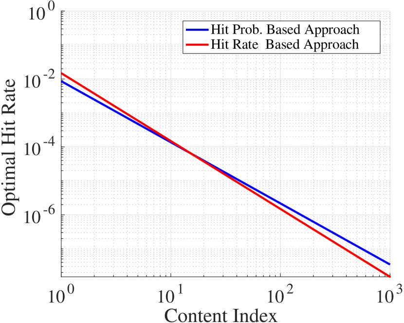
(a)

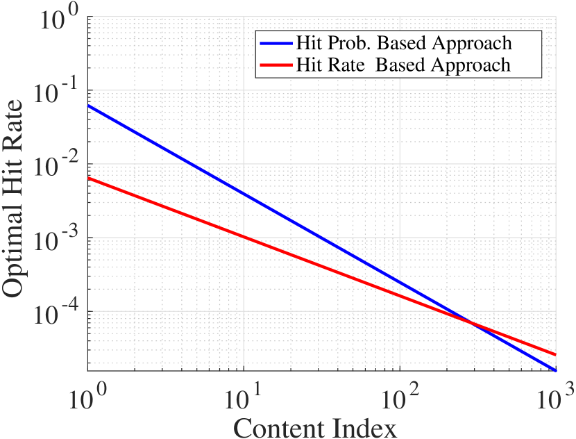
(b)

Figure 1. HRB-CUM vs. HPB-CUM under exponential distribution: (a) $\beta=0.8$ and (b) $\beta=2.$

Figures 1 (a) and (b) illustrate the case that $w_{i}=\mu_{i}$, $\beta=0.8$ and $\beta=2$, respectively. We consider the Zipf popularity distribution with parameter $\alpha=0.8$, $n=10^{3}$ and $B=100$ in our numerical studies.

We make a similar comparison of the hit probabilities under HRB-CUM and HPB-CUM.

Theorem 5.

When $w_{1}\geq\cdots\geq w_{n},$ (i) for $\beta<1,$ $\exists j\in(1,n)$ s.t. $h^{r}_{i}>h^{p}_{i},$ $\forall i<j$, and $h^{r}_{i}<h^{p}_{i},$ $\forall i>j;$ and (ii) for $\beta>1,$ $\exists l\in(1,n)$ s.t. $h^{r}_{i}<h^{p}_{i},$ $\forall i<l$, and $h^{r}_{i}>h^{p}_{i},$ $\forall i>l.$ In particular, if $j,l\in\mathbb{Z}^{+},$ then $h^{r}_{j}=h^{p}_{j},$ and $h^{r}_{l}=h^{p}_{l}.$

The following corollary applies to the Zipf popularity distribution.

Corollary 0.

If the popularity distribution is Zipfian: (a)$h^{r}_{i}>h^{p}_{i},$ for $i=1,\cdots,i_{0},$ and $h^{r}_{i}<h^{p}_{i},$ for $i=i_{0}+1,\cdots,n$ when $\beta<1;$ (b)$h^{r}_{i}<h^{p}_{i},$ for $i=1,\cdots,i_{0},$ and $h^{r}_{i}>h^{p}_{i},$ for $i=i_{0}+1,\cdots,n,$ where $i_{0}=\Bigg{\lfloor}\left(\frac{\sum_{j}w_{j}^{\frac{1}{\beta}}j^{\alpha(1-\frac{1}{\beta})}}{\sum_{j}w_{j}^{\frac{1}{\beta}}}\right)^{\frac{1}{\alpha(1-\frac{1}{\beta})}}\Bigg{\rfloor},$ when $\beta>1.$

We numerically verify our results, and observe that they exhibit similar trends as in Figures 1 (a) and (b), hence we omit them here due to space constraints.

We are unable to achieve explicit expressions for $h^{r}_{i}$, $h^{p}_{i}$, $\lambda^{r}_{i}$ and $\lambda_{i}^{p}$ for HRB-CUM and HPB-CUM when inter-request times are characterized by other distributions. However, from Section 4, we know that HRB-CUM and HPB-CUM are convex optimization problems when the distribution is DHR. We numerically compare the performance of HRB-CUM and HPB-CUM under a Zipf-like distribution with parameter $\alpha=0.8$. Similar results as that of the Poisson request process hold for these distributions, and we omit the results due to space limitation.

6. Decentralized Algorithms

In Section 3, we formulated an optimization problem with a fixed cache size under the assumption of a static known workload. However, system parameters (e.g. request processes) can change over time, and as discussed in Section 4, the optimization problem under some inter-request distributions cannot easily be solved. Moreover, it is infeasible to solve the optimization problem offline and then implement the optimal strategy. Hence decentralized algorithms are needed to implement the optimal strategy to adapt to these changes in the presence of limited information.

Remark 4.

Note that, the proposed decentralized algorithms only require local information (such as irt distribution parameters for that particular content) to achieve global optimality whereas the centralized algorithm requires information about all content request processes.

In the following, we develop decentralized algorithms for HRB-CUM and compare their performance to those for HPB-CUM under stationary request processes discussed in Section 4. We only present explicit algorithms for HRB-CUM, similar algorithms for HPB-CUM are available in Appendix 11.5. We drop the superscript $r$ in this section for brevity.

6.1. Dual Algorithm

For a request arrival process with a DHR inter-request time distribution, (10) becomes a convex optimization problem as discussed in Section 4, and hence solving the dual problem produces the optimal solution. Since $0<t_{i}<\infty,$ then $0<\lambda_{i}/\mu_{i}<1$ and $0<g_{i}(\lambda_{i}/\mu_{i})<1.$ Therefore, the Lagrange dual function is

(25) $$D(\eta)=\max_{\lambda_{i}}\left\{\sum_{i=1}^{n}U_{i}(\lambda_{i})-\eta\left[\sum_{i=1}^{n}g_{i}\left(\lambda_{i}/\mu_{i}\right)-B\right]\right\},$$

and the dual problem is

(26) $$\min_{\eta\geq 0}\quad D(\eta).$$

Following the standard gradient descent algorithm by taking the derivative of $D(\eta)$ w.r.t. $\eta,$ the dual variable $\eta$ should be updated as

(27) $$\eta^{{(k+1)}}\leftarrow\max\left\{0,\eta^{{(k)}}+\gamma\left[\sum_{i=1}^{n}g_{i}(\lambda_{i}^{(k)}/\mu_{i})-B\right]\right\},$$

where $k$ is the iteration number, $\gamma>0$ is the step size at each iteration and $\eta\geq 0$ due to KKT conditions.

Based on the results in Section 3, in order to achieve optimality, we must have

(28) $$\eta^{{(k)}}=\frac{\mu_{i}U_{i}^{\prime}(\lambda_{i}^{(k)})}{g_{i}^{\prime}(\lambda_{i}^{(k)}/\mu_{i})}\triangleq y_{i}(\lambda_{i}^{(k)}/\mu_{i}),\;\text{i.e.},\;\lambda_{i}^{{(k)}}=\mu_{i}y_{i}^{-1}(\eta^{{(k)}}).$$

Since $g_{i}(\lambda_{i}^{(k)}/\mu_{i})$ indicates the probability that content $i$ is in the cache, $\sum_{i=1}^{n}g_{i}(\lambda_{i}^{(k)}/\mu_{i})$ represents the number of contents currently in the cache, denoted as $B_{\text{curr}}$. Therefore, the dual algorithm for a reset TTL cache is

(29a) $$t_{i}^{(k)}=F_{i}^{-1}(y_{i}^{-1}(\eta^{{(k)}})),$$

(29b) $$\eta^{{(k+1)}}\leftarrow\max\left\{0,\eta^{{(k)}}+\gamma(B_{\text{curr}}-B)\right\},$$

which is executed every time a request is made.

Remark 5.

From (28) and (29), it is clear that if the explicit form of $g_{i}(\cdot)$ or $g_{i}^{\prime}(\cdot)$ is available, then the dual algorithm can be directly implemented. This is the case for Poisson and generalized Pareto inter-request distributions, see Section 4 and the following for details. However, neither is available for the hyberexponential distribution and the $2$-MMPP. In the following, we will show that the dual algorithm can still be implemented without this information.

Poisson Process: We have $g^{\prime}_{i}(\lambda_{i}^{(k)}/\mu_{i})=1,$ and $\lambda_{i}^{(k)}=U_{i}^{\prime-1}(\eta^{{(k)}}/\mu_{i}).$

Generalized Pareto Distribution: When inter-request times are described by a generalized Pareto distribution and utilities are $\beta$-fair, $\lambda_{i}^{{(k)}}$ is the solution of

(30) $$\mu_{i}^{1-\beta}w_{i}(1-(\lambda_{i}^{(k)}/\mu_{i}))^{k_{i}}/[\eta^{(k)}(1-k_{i})]-(\lambda_{i}^{(k)}/\mu_{i})^{\beta}=0.$$

We can show that there exists a solution in $[0,\mu_{i}]$ for any $\eta^{{(k)}}>0$; details are given in Appendix 11.5.1.

Hyperexponential Distribution: Under a hyperexponential distribution, we have $g^{\prime}_{i}(x)=\mu_{i}(1-x)/f_{i}(F_{i}^{-1}(x)).$ Since we do not have a closed form expression for $F_{i}^{-1}(x)$, no explicit form exists for $g^{\prime}_{i}(x)$. Given (28) and a $\beta$-fair utility, timer $t_{i}^{{(k)}}$ is obtained as a solution of the following fixed point equation

(31) $$(F_{i}(t_{i}^{(k)}))^{\beta+1}-(F_{i}(t_{i}^{(k)}))^{\beta}+f_{i}(t_{i}^{(k)})/[\eta^{{(k)}}\mu_{i}^{\beta-1}]=0,$$

where $F_{i}(t)=1-\sum\limits_{j=1}^{l}p_{ji}e^{-\theta_{ji}t}$ and $f_{i}(t)=\sum\limits_{j=1}^{l}p_{ji}\theta_{ji}e^{-\theta_{ji}t}.$

$2$-MMPP: From Section 4, the inter-request times of a $2$-MMPP are described by a second order hyperexponential distribution. Hence timer $t_{i}^{{(k)}}$ can be updated from (31) with $F_{i}(t)=1-\sum_{j=1}^{2}q_{ji}e^{-u_{ji}t}$ and $f_{i}(t)=\sum_{j=1}^{2}q_{ji}u_{ji}e^{-u_{ji}t}.$

Remark 6.

We can similarly design primal and primal-dual algorithms by adding a convex and non-decreasing cost function $C(\cdot)$ to the sum of utilities, denoting the cost for extra cache storage. For ease of exposition, we relegate their description to Appendix 11.5.2. In the remainder of the paper, we refer to these distributed algorithms as Dual, Primal and Primal-Dual, respectively.

6.2. Performance Evaluation

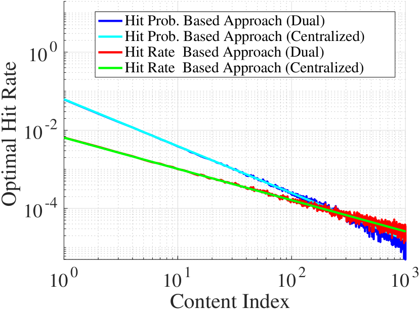
(a)

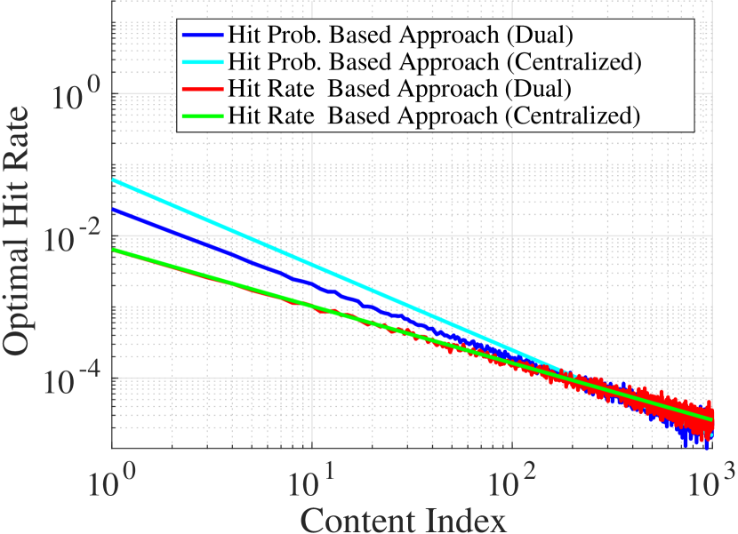
(b)

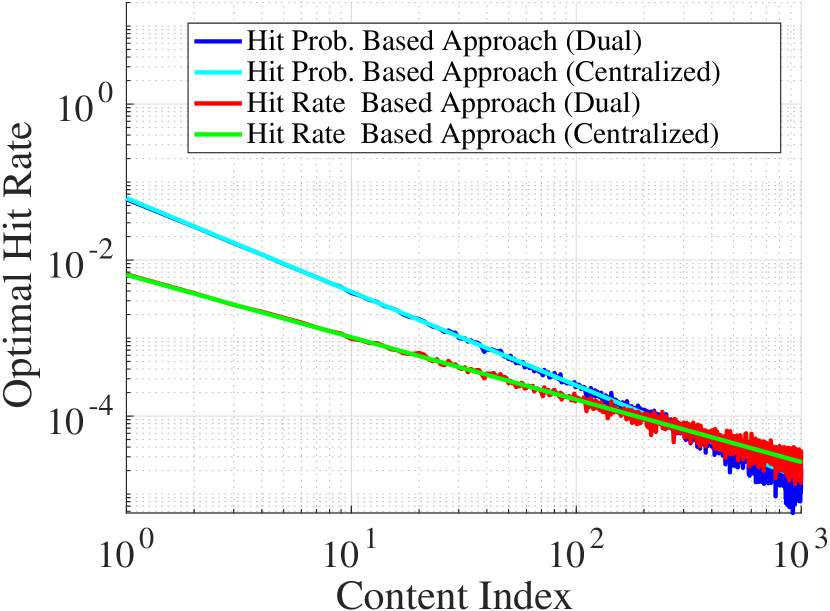
(c)

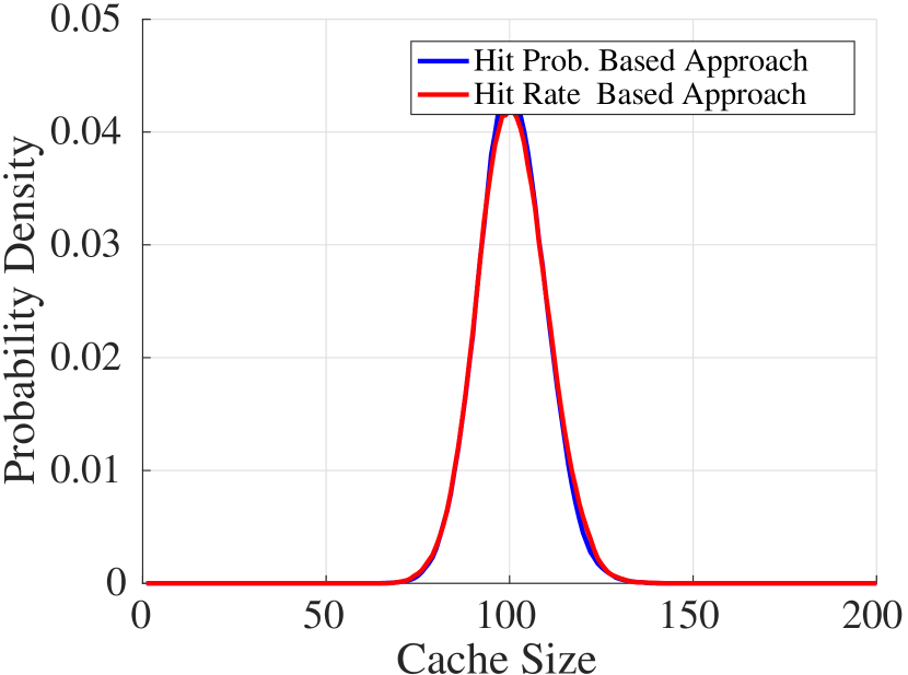
(d)

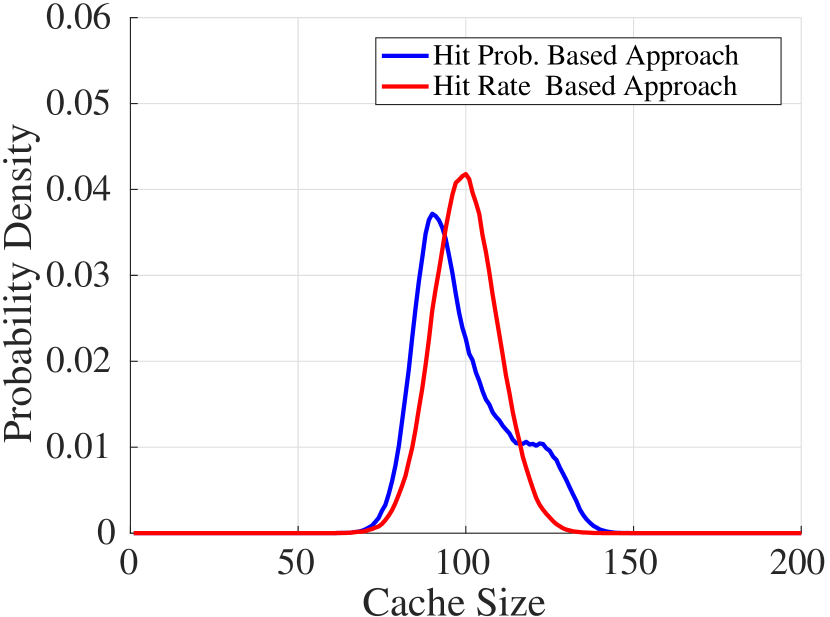
(e)

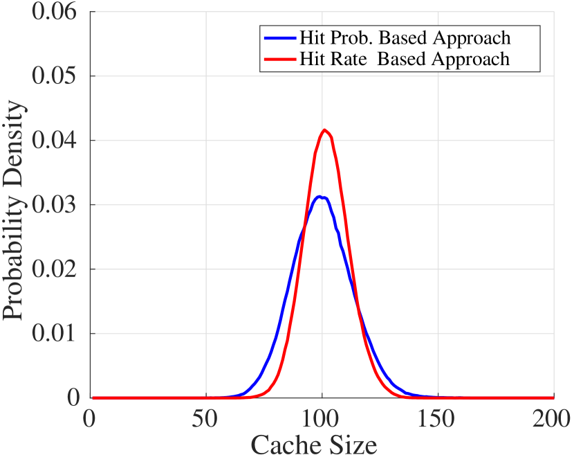
(f)

Figure 2. Dual for HRB-CUM and HPB-CUM with under exponential distribution with minimum potential delay fairness; Hit rate (Fig. $a$-$c$) and cache size distribution (Fig. $d$-$f$) comparisons for Dual with $\gamma=10^{-7}$ ($a,d$), $\gamma=10^{-3}$ ($b,e$) and $\gamma=10^{-5}$ ($c,f$) under exponential inter-request process.

In this Section, we evaluate the performance of the decentralized algorithms for both HRB-CUM and HPB-CUM when inter-request times are described by stationary request processes with an exponential irt distribution when utility functions are $\beta$-fair. Due to space restrictions, we limit our study to minimum potential delay fairness, i.e., $\beta=2$.

6.2.1. Experiment Setup

In our studies, we consider a Zipf popularity distribution with $\alpha=0.8,$ $n=1000$ and $B=100.$ We consider the inter-request time distributions described in Section 4 with an aggregate request rate $\mu=1$ such that $\mu_{i}=p_{i}$ from (4). In particular, for exponential distribution, the rate parameter is set to $\mu_{i}=p_{i}$. We relegate discussions of generalized Pareto, hyperexponential and $2$-MMPP to Section 8

6.2.2. Exactness

We first consider the dual algorithm described in Section 6.1. Note that the dual algorithm for generalized Pareto involves solving nonlinear equation (30). We solve it efficiently with Matlab routine fsolve using a step size $\gamma=10^{-7}.$ The performance of dual under exponential is shown in Figure 2 ($a$), where “Centralized” means solutions from solving (10).

From Figure 2 ($a$), we observe that the decentralized algorithms yield the exact hit rates under both HRB-CUM and HPB-CUM. Similarly results hold for hit probabilities, omitted here due to space limits. Figure 2 ($d$) shows the probability density for the number of contents in the cache across these distributions. As expected the density is highly concentrated around the cache size $B$. Similar results hold for generalized Pareto distribution and we omit the results due to space limits.

We also use primal and primal-dual distributed algorithms to implement minimum potential delay fairness. In particular, as discussed in Section 6, primal is associated with a penalty function $C(\cdot)$. Choosing an appropriate penalty function plays an important role in the performance of primal, since we need to evaluate the gradient at each iteration through $C^{\prime}(\cdot)$. Here, we use $C(x)=\max\{0,x-B\log(B+x)\}$ (Srikant and Ying, 2013). Another reasonable choice can be $C(x)=\max\{0,x^{m}\},\;m\geq 1$. We observe that both primal and primal-dual yield exact hit probabilities and hit rates under HRB-CUM and HPB-CUM for minimum potential delay fairness. We omit the plots due to space constraints.

6.2.3. Convergence Rate and Robustness

Although the decentralized algorithms converge to the optimal solution as shown in Section 6.2.2, the rate of convergence is also important from a service provider’s perspective. Due to space limits, we only focus on the dual here. From (29), it is clear that the step size $\gamma^{p}$ (or $\gamma^{r}$) plays a significant role in the convergence rate. We choose different values of $\gamma^{p}$ and $\gamma^{r}$ and compare the performance of HRB-CUM and HPB-CUM under Poisson request processes, shown in Figure 2 ($b$) and ($c$). On one hand, we find that when a larger value of $\gamma^{p}=\gamma^{r}=10^{-3}$ is chosen, the dual for HRB-CUM easily converges after a few iterations (more than a few $5\times 10^{5}$ iterations), i.e., the simulated hit rates exactly match numerically computed values, while those of HPB-CUM do not converge. On the other hand, when a smaller value $\gamma^{p}=\gamma^{r}=10^{-5}$ is chosen, both converge in the same number of iterations. We also used $\gamma^{p}=\gamma^{r}=10^{-1},10^{-7}$, which exhibit similar behaviors to $10^{-3}$ and $10^{-5},$ respectively, and are omitted due to space constraints.

We also explored the expected number of contents in the cache, shown in Figure 2 ($e$) and ($f$). It is obvious that under HRB-CUM, the probability of violating the target cache size $B$ is quite small, while it is larger for HPB-CUM especially for $\gamma^{p}=\gamma^{r}=10^{-3},$ and even for $\gamma^{p}=\gamma^{r}=10^{-5},$ HRB-CUM is more concentrated on the target size $B.$ These results indicate that the dual algorithm associated with HRB-CUM is more robust to changes in the step size and converges much faster under exponential inter-requests.

6.2.4. Comparison of Decentralized Algorithms

From the above analysis, we know that at each iteration, the dual algorithm needs to solve a non-linear equation to obtain a timer value, which might be computationally intensive compared to primal and primal-dual. However, for primal, some choices of penalty function $C(\cdot)$ and arrival process $g_{i}(\cdot)$ may result in large gradients and abrupt function change (Smith and Coit, 1996). Similarly for primal-dual, two scaling parameters $\delta_{i}$ and $\gamma$ need to be carefully chosen, otherwise the algorithm might diverge. These demonstrate the pro-and-cons of these distributed algorithms, and one algorithm may be favorable than others in specific situations.

7. Stability Analysis of Decentralized Algorithms

In this section, we derive stability results for the decentralized algorithms proposed in Section 6.1. In particular, we establish stability of the update rule (27) around its equilibrium $\eta^{*}.$ A continuous time approximation to (27) was studied in (Dehghan et al., 2016) and for it, stability results were established using Lypaunov theory. Motivated by the fact that this approximation is neither necessary nor sufficient for the stability of the actual discrete-time update rule (27), we propose to analyze its stability directly in the discrete time domain. W.l.o.g., we consider the log utility function. We assume requests for each content arrive according to a Poisson process and give conditions on $\gamma$ guaranteeing stability of the update rule (27). We also perform stability analysis with other irt distributions, such as Pareto distribution, as discussed in Appendix 11.7.

7.0.1. Local stability analysis

When requests arrive according to a Poisson process we have

(32) $$D(\eta) =\sum_{i=1}^{n}w_{i}\log(\mu_{i}w_{i}/\eta)-\eta\left[\sum_{i=1}^{n}w_{i}/\eta-B\right]=\overline{W}-W\log(\eta)-W+\eta B,$$

where $\overline{W}=\sum_{i=1}^{n}w_{i}\log(\mu_{i}w_{i})$ and $W=\sum_{i=1}^{n}w_{i}.$ Let $\eta^{*}=W/B$ be the unique minimizer of the dual function $D(\eta)$ defined in (32). We have the following dual algorithm.

(33) $$\eta^{(k+1)}\leftarrow\max\left\{0,\eta^{(k)}+\gamma\left(W/\eta^{(k)}-B\right)\right\}.$$

Any differentiable function $f(\eta)$ can be linearized around a point $\eta^{*}$ as $L(\eta)=f(\eta^{*})+f^{\prime}(\eta^{*})(\eta-\eta^{*}).$ Denote $f(\eta)=\eta+\gamma\left(W/\eta-B\right)$ with $f:\mathbb{R}^{+}\rightarrow\mathbb{R}.$ We have $f(\eta^{*})=\eta^{*}$. We also know that $\eta^{*}=W/B.$ Under linearization, substituting $f^{\prime}(\eta^{*})=1-(\gamma B^{2}/W)$ in $L(\eta)$ we get

(34) $$\eta^{(k+1)}=\eta^{*}+\left(1-\frac{\gamma B^{2}}{W}\right)(\eta^{(k)}-\eta^{*}).$$

Denote $\eta_{\delta}^{(k)}=\eta^{(k)}-\eta^{*}$ as deviation from $\eta^{*}$ at $k^{th}$ iteration. Hence we have

(35) $$\eta_{\delta}^{(k+1)}=\left(1-\frac{\gamma B^{2}}{W}\right)\eta_{\delta}^{(k)}=\left(1-\frac{\gamma B^{2}}{W}\right)^{k}\eta_{\delta}^{(0)}.$$

and (34) is locally asymptotically stable if

(36) $$\gamma<\frac{2W}{B^{2}}.$$

Thus, if (36) holds, then the update rule (27) converges to $\eta^{*}$ as long as $\eta^{(0)}$ is sufficiently close to $\eta^{*}$.

7.0.2. Global stability guarantees

In (Dehghan et al., 2016), a Lyapunov function was constructed for a continuous-time approximation to (27). Now, we consider a discrete-time Lyapunov candidate $V(\eta)=D(\eta)-D(\eta^{*})$ for (27) directly. By discrete time Lyapunov function theory (Hahn, 1958), for global asymptotic stability, we must have $V(f(\eta))-V(\eta)<0,\forall\;\eta>0,\eta\neq\eta^{*}$ and for some candidate Lyapunov function $V.$ We evaluate $\Delta V(\eta)=V(f(\eta))-V(\eta)$ with $V(\eta)=D(\eta)-D(\eta^{*}).$

$$\Delta V(\eta) =V(f(\eta))-V(\eta)=D(f(\eta))-D(\eta)=-W\log(f(\eta))+f(\eta)B+W\log\eta-\eta B,$$

(37) $$=-W\log\left[1+\frac{\gamma}{\eta}\bigg{(}\frac{W}{\eta}-B\bigg{)}\right]+B\gamma\left(\frac{W}{\eta}-B\right).$$

Here, we are interested in finding a scaling parameter such that $\Delta V(\eta)<0$ for all $\eta>0$ thereby proving that the online algorithm (27) is stable for any initial starting value $\eta^{(0)}$. We consider two cases: where $\gamma$ is constant and another when $\gamma$ is a function of the dual variable.

Scaling Parameter as a function of dual variable: We consider the case $\gamma=\gamma(\eta)$ such that the update rule (27) is globally stable around its equilibrium $\eta^{*}.$ Such a function is constructed in Appendix 11.6.

Constant Scaling Parameter: When $\gamma$ is fixed, independent of $\eta,$ we can show that $V$ is not a Lyapunov function. We consider the following theorem.

Theorem 1.

Given $\gamma>0$, $\Delta V(\eta)>0\;\forall\;\eta<\eta^{*}$.

From Theorem 1, it is clear that when $\gamma$ is independent of $\eta$, the candidate Lyapunov function: $V(\eta)=D(\eta)-D(\eta^{*})$ cannot guarantee global asymptotic stability. See proof in Appendix 11.8.

8. Poisson Online Approximation

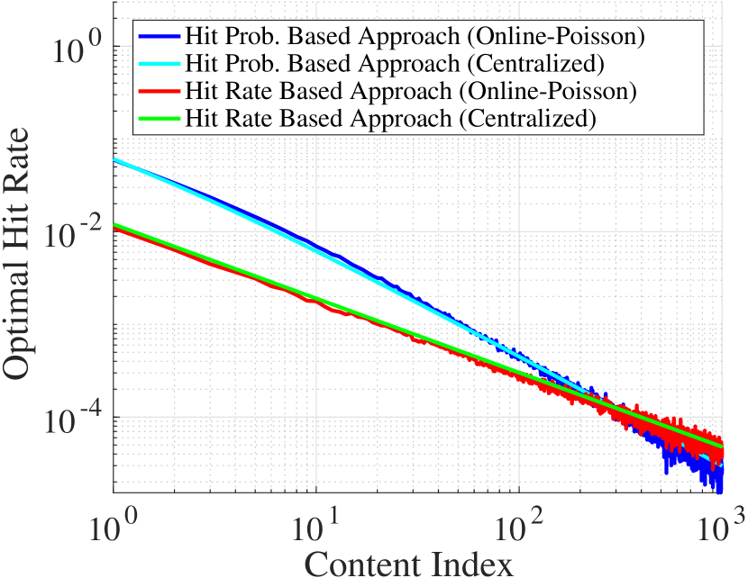
Figure 3. Poisson online approximation to Generalized Pareto inter-requests.

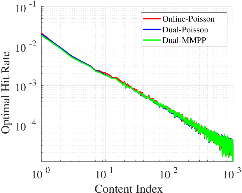
Figure 4. Poisson online approximation to 2-MMPP inter-requests: $x=10^{-3}$.

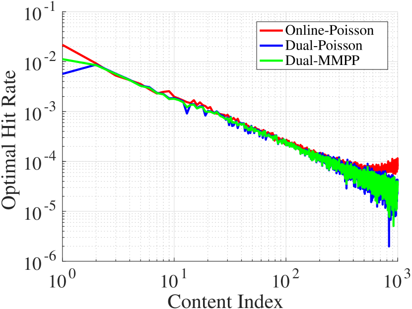
Figure 5. Poisson online approximation to 2-MMPP inter-requests: $x=10^{-7}$.

From Section 6, it is clear that the implementation of Dual under generalized Pareto, hyperexponential distributions and $2$-MMPP involves solving non-linear fixed point equations, which are computationally intensive. However, the Dual for the case of requests governed by Poisson processes is simple. Furthermore, knowledge of the inter-request distribution is also required. However, this is not always available to the service provider.

In this section, we apply the Dual designed for Poisson request processes to a workload where requests are described by a non-Poisson stationary request processes. Such an algorithm does not require solving non-linear equations and hence is computationally efficient. Moreover, we also use estimation techniques introduced in (Dehghan et al., 2016) to approximate request rates which makes these distributed algorithms work in an online fashion.

8.1. Online Algorithm

We consider the problem of estimating the arrival rate $\mu_{i}$ for content $i$ adopting techniques used in (Dehghan et al., 2016) described as follows. Denote the remaining TTL time for content $i$ as $\tau_{i}$. This can be computed given $t_{i}$ and a time-stamp for the last request time for content $i.$ Recall that $X_{ik}$ is a random variable corresponding to the inter-request times for requests for content $i.$ Let $\bar{X}_{ik}$ be the mean. Then we approximate the mean inter-request time as $\hat{\bar{X}}_{ik}=t_{i}-\tau_{i}.$ Clearly $\hat{\bar{X}}_{ik}$ is an unbiased estimator of $\bar{X}_{ik}$, and hence an unbiased estimator of $1/\mu_{i}.$ In this section, we use this estimator to implement the distributed algoritms, which now becomes an online algorithm.

Given this estimator and Dual (29), we propose the following Poisson approximate online algorithm

(38a) $$t_{i}^{(k)}=-\frac{1}{\hat{\mu}_{iP}}\log\Bigg{(}1-\frac{1}{\hat{\mu}_{iP}}U_{i}^{\prime-1}\left(\frac{\eta^{(k+1)}}{\hat{\mu}_{iP}}\right)\Bigg{)},$$

(38b) $$\eta^{{(k+1)}}\leftarrow\max\{0,\eta^{{(k)}}+\gamma(B_{\text{curr}}-B)\}.$$

There are two differences between our proposed algorithm (38) and Dual (29). First, the explicit form of (29a) is different for different inter-request distributions as discussed in Section 6.1, while we always adopt the explicit form of Poisson process in (38a). Second, $\mu_{i}$ in (28) is the exact value of the mean arrival rate of the corresponding inter-request distribution, while we estimate its value as discussed above and denote it as $\hat{\mu}_{iP}.$ However, the value of $B_{\text{curr}}$ denotes the number of contents currently in the cache under the real inter-request distribution under both (38) and (29). In the following, we consider the performance of (38) under different inter-request distributions.

8.2. Generalized Pareto Distribution

In this section, we apply the online algorithm (38) to a workload where requests are described by stationary request process under generalized Pareto distribution with shape parameter $k_{i}=0.48.$ The performance is shown in Figure 5 . It is clear that the approximation is accurate. Furthermore, it has been theoretically characterized in (Weinberg, 2016) that for any given generalized Pareto model with finite variance, the exponential approximation that minimizes the K-L divergence between these two distributions has the same mean as that of the generalized Pareto distribution, i.e. $\mu_{i}=(1-k_{i})/\sigma_{i}$. The estimator we use in our online algorithm (38), i.e., $1/\hat{\mu}_{iP}$, is an unbiased estimator of mean inter-request time of the generalized Pareto arrival process, thus explaining the better performance of our Poisson approximation in accordance with the theoretical results provided in (Weinberg, 2016). Moreover, we notice that when $k_{i}$ becomes smaller, the accuracy has been improved. However, this approximation has poor performance when $k_{i}>0.5$ since the generalized Pareto distribution has infinite variance for $k_{i}>0.5.$

8.3. $m$-state MMPP

Under the general $m$-state MMPP, we can theoretically characterize the limit behaviors of the irts. W.l.o.g. denote the transition rate for content $i$ from state $j$ to $k$ as $r_{jki}$. Let $Q_{i}=[r_{jki},1\leq j\leq m,1\leq k\leq m],$ be the corresponding generator matrix. Arrivals for content $i$ at state $j$ are described by a Poisson process with rate $\theta_{ji}$. Then the steady state distribution, $\pi_{i}=[\pi_{ji},1\leq j\leq m]$, satisfies $\pi_{i}Q_{i}=0$. We represent $r_{jki}=a_{jki}x_{i}$, where $a_{jki}$ are constants, and $0\leq x_{i}\leq\infty.$ We summarize the results in the following theorems and relegate the proofs to 11.11.

Theorem 1.

When $r_{jki}\rightarrow 0$, i.e., $x_{i}\rightarrow 0$, the inter-request times are described by an $m^{th}$ order hyperexponential distribution.

Theorem 2.

When $r_{jki}\rightarrow\infty$, i.e., $x_{i}\rightarrow\infty$, the inter-request times are exponentially distributed with mean arrival rate

(39) $$\bar{\theta}_{i}=\sum_{j=1}^{m}\theta_{j}\pi_{ji}.$$

i.e., $m$-MMPP is equivalent to a Poisson process with rate $\bar{\theta}_{i}$, i.e., our approximation is exact.

Since there is no explicit form of the inter-request time distribution for a general $m$-state MMPP, we focus on a $2$-MMPP in our numerical studies.

8.3.1. 2-MMPP

The optimal hit rates under $2$-MMPP can be obtained through solving Dual for a second order hyperexponential distribution with parameters $q,u_{1}$ and $u_{2}$ defined in (4). However, from Section 6, Dual requires solving a non-linear equation (31). Instead, we consider Poisson approximation (38) under $2$-MMPP. W.l.o.g., we assume the phase rates $\theta_{1i}$ and $\theta_{2i}$ for $i=1,\cdots,n$ to be Zipf distributed with parameters $0.4$ and $0.8,$ respectively.

Limiting Behavior: We first evaluate the performance of Poisson online approximation algorithm (38) for different transition rates $r_{12i}$ and $r_{21i}$.

Theorem 3.

(1) When $r_{12i},r_{21i}\rightarrow\infty$, i.e., $x_{i}\rightarrow\infty$, $2$-MMPP is equivalent to a Poisson process with rate $\frac{\theta_{1i}a_{21i}+\theta_{2i}a_{12i}}{a_{12i}+a_{21i}}$, i.e., our approximation is exact.

(2) When $r_{12i},r_{21i}\rightarrow 0$, i.e., $x_{i}\rightarrow 0$,

(40) $$u_{1i}\rightarrow\theta_{2i},\quad u_{2i}\rightarrow\theta_{1i},\quad q_{1i}\rightarrow\frac{\theta_{2i}a_{12i}}{\theta_{1i}a_{21i}+\theta_{2i}a_{12i}},\quad q_{2i}\rightarrow\frac{\theta_{1i}a_{21i}}{\theta_{1i}a_{21i}+\theta_{2i}a_{12i}},$$

The proof is relegated to Appendix 11.10.

Numerical Validation: We numerically verify the results in Theorem  3 by taking different values of transition rates. The performance comparison between two limiting cases are shown in Figures 5 and 5, respectively,where “Dual-MMPP” is obtained from Dual (29) in Section 6, “Dual-Poisson” is obtained from (38) with the exact mean $\mu_{i}=(\theta_{1i}r_{21i}+\theta_{2i}r_{12i})/(r_{12i}+r_{21i})$ is known and “Online-Poission” is obtained from (38) with estimated arrival rates as discussed in Section 8.1. We can see that with large transition rates, the Poisson approximation performs better as compared to small transition rates. This is due to the fact that our approximation becomes exact when transition rates go to infinity. However, our approximation yields similar optimal aggregate hit rate as compared to “Dual-MMPP” even for small transition rates as shown in Table 2. We also numerically verify the case for intermediate transition rates by taking $r_{12i}=5\times 10^{-5}$ and $r_{21i}=2\times 10^{-5}.$ Again, we can see that the optimal hit rates obtained through (38) match those obtained from Dual under $2$-MMPP. We omit the plot due to space limits.

$x$	$n$	$B$	Dual-MMPP	Dual-Poisson	Online-Poisson
$10^{-3}$	$1000$	$100$	$0.1591$	$0.1612$	$0.1655$
$10^{-7}$	$1000$	$100$	$0.1474$	$0.1427$	$0.1540$

Table 2. Optimal aggregate hit rates for large ($x=10^{-3}$) and small ($x=10^{-7}$) state transition rates.

Remark 7.

We also considered the case when irts follow hyperexponential and weibull distributions. Equation  (10) can be solved with Dual for both distributions. We compare results using  (10) with those obtained using  (38) and we find that the optimal hit rates obtained through (38) match those obtained solving  (10). For ease of exposition, these results are relegated to Appendix 11.9.

9. Trace-driven Simulation

In this section, we evaluate the accuracy of the reverse engineered dual implementation of LRU and compare the performance of LRU to that of Poisson approximate online algorithm through trace-driven simulation. We use requests from a web access trace collected from a gateway router at IBM research lab (Zerfos et al., 2013). The trace contains $3.5\times 10^{6}$ requests with a content catalog of size $n=5638.$ We consider a cache size $B=1000.$

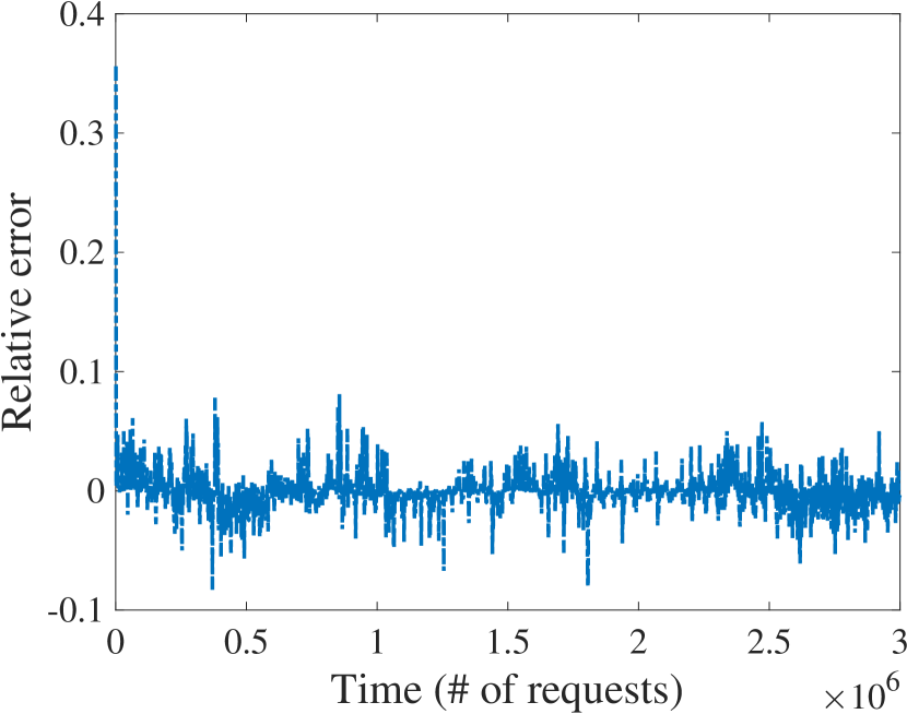
Figure 6. Relative error in hit counts of LRU and the reverse engineered dual algorithm.

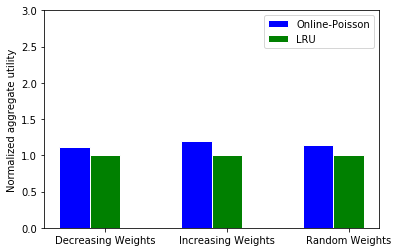
Figure 7. Trace-driven comparison for online-Poisson and LRU caching policy.

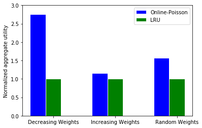
Figure 8. Synthetic trace-driven comparison for online-Poisson and LRU caching policy.

9.1. Reverse Engineering

We use the trace to compute cache hits for the replacement-based implementation of LRU and the implementation based on reverse engineered dual algorithm. We count the number of hits from each implementation over windows of $3000$ requests and compute the relative error. From Figure 8, it is clear that the relative error is small over time. Thus the implementation based on the reverse engineered dual algorithm performs close to its replacement-based implementation.

9.2. Effect of content weights

The utility function defined in (7) involves content weights, $w_{i}$, associated with each content $i.$ Classical cache replacement policies such as LRU are oblivious to content weights. However, the Poisson approximation based online algorithm updates the TTL timer by considering the content weight at each time step. Thus the Poisson approximation based online algorithm is more robust to variation in content weights. Figure 8 compares the performance of online Poisson algorithm to that of LRU across different sets of content weights, i.e. we consider the following three cases: (a) $w_{i}=\mu_{i}$ (decreasing weights and decreasing request rates) (b) $w_{i}=1/\mu_{i}$ (increasing weights and decreasing request rates) (c) $w_{i}=\texttt{rand}(0,1)$ (random weights and decreasing request rates). Let $U_{P}$ and $U_{L}$ denote the aggregate content utility for online Poisson algorithm and for LRU policy, respectively. We normalize both utilities w.r.t. LRU policy as $U_{P}/U_{L}$ and $U_{L}/U_{L}=1$, respectively. From Figure 8, it is clear that in each case online Poisson algorithm performs better than LRU, i.e. online Poisson algorithm achieves larger aggregate utility as compared to the LRU policy.

We also consider a synthetic trace generated with a content catalog of size $n=1000$ and irt distribution following a generalized Pareto distribution. The results are shown in Figure 8. It is clear from Figure 8 that the Poisson approximation based online algorithm performs even better as compared to LRU when the request process is stationary. We also get similar performance benefits when compared to other classical replacement based caching policies such as FIFO and RANDOM. We omit them due to space constraints.

10. Conclusion

In this paper, we associated each content with a utility that is a function of the corresponding content hit rate or hit probability, and formulated a cache utility maximization problem under stationary requests. We showed that this optimization problem is convex when the request process has a DHR. We presented explicitly optimal solutions for HRB-CUM and HPB-CUM, and made a comparison between them both theoretically and numerically. We also developed decentralized algorithms to implement the optimal policies. We found that HRB-CUM is more robust and stable than HPB-CUM w.r.t. convergence rate. Finally, we proposed Poisson approximate online algorithms to different inter-request distributions, which is accurate and lightweight. Going further, we aim at extending our results to consider Non-reset TTL Cache where the timer is set only on a cache miss. Non-reset TTL Caches might have different implications on the design and performance analysis of distributed and online algorithms. Establishing these results will be our future goal.

11. Appendix

11.1. HPB-CUM

Following a similar argument in Section 3, we can formulate the following hit probability based optimization problem

(41) $$\text{\bf{HPB-CUM:}}\quad\max_{0\leq h_{i}^{p}\leq 1}\sum_{i=1}^{n}U_{i}(h_{i}^{p}),\quad\text{s.t.}\sum_{i=1}^{n}g_{i}(h_{i}^{p})\leq B,$$

The Lagrangian function can be written as

(42) $$\mathcal{L}^{p}(\boldsymbol{h}^{p},\eta^{p})=\sum_{i=1}^{n}U_{i}(h_{i}^{p})-\eta^{p}\left[\sum_{i=1}^{n}g_{i}(h_{i}^{p})-B\right],$$

where $\eta^{p}$ is the Lagrangian multiplier and $\boldsymbol{h}^{p}=(h_{1}^{p},\cdots,h_{n}^{p})$. Similarly, the derivative of $\mathcal{L}^{p}(\boldsymbol{h}^{p},\eta^{p})$ w.r.t. $h_{i}^{p}$ for $i=1,\cdots,n,$ should satisfy the following condition so as to achieve its maximum

(43) $$\eta^{p}=U_{i}^{\prime}(h_{i}^{p})/g^{\prime}_{i}(h_{i}^{p})\triangleq v_{i}(h_{i}^{p}),$$

where $v_{i}(\cdot)$ is a continuous and differentiable function on $[0,1],$ i.e., there exists a one-to-one mapping between $\eta^{p}$ and $h_{i}^{p}$ if $0\leq v_{i}^{-1}(\eta^{p})\leq 1.$ Again, by the cache capacity constraint, we can compute $\eta^{p}$ through the following fixed-point equation

(44) $$\sum_{i=1}^{n}g_{i}(h_{i}^{p}) =\sum_{i=1}^{n}g_{i}(v_{i}^{-1}(\eta^{p}))=B.$$

Finally, given $\eta^{p}$, the timer, hit probability, and hit rate are

(45) $$t_{i}=F_{i}^{-1}(v_{i}^{-1}(\eta^{p})),\quad h_{i}^{p}=v_{i}^{-1}(\eta^{p}),\quad \lambda_{i}^{p}=\mu_{i}v_{i}^{-1}(\eta^{p}),\quad i=1,\cdots,n.$$

11.2. Proofs in Section 3

11.2.1. Convexity of HRB-CUM (8) and HPB-CUM (41)

In this section, we show that HRB-CUM (8) and HPB-CUM (41) in terms of timers are non-convex.

Theorem 0.

HRB-CUM (8) and HPB-CUM (41) in terms of timers are non-convex.

Proof.

Recall that

$$\hat{F}_{i}(t_{i})=\mu_{i}\int_{0}^{t_{i}}(1-F(x))dx.$$

Take the derivative w.r.t. $t_{i},$ we have

(46) $$\frac{\partial\hat{F}_{i}(t_{i})}{\partial t_{i}}=\mu_{i}(1-F(t_{i})),\quad\text{and}\quad\frac{\partial^{2}\hat{F}_{i}(t_{i})}{\partial t_{i}^{2}}=-\mu_{i}f_{i}(t_{i}).$$

Since $f_{i}(\cdot)$ is the p.d.f. for the inter-request arrival time with $\mu_{i}\geq 0$, we have $f_{i}(t_{i})\geq 0.$ Thus $\partial^{2}\hat{F}_{i}(t_{i})/\partial t_{i}^{2}\leq 0.$ Therefore, $\hat{F}_{i}(t_{i})$ is concave in $t_{i}$ and then (8) is a non-convex optimization problem. Similarly, we can show that (41) is non-convex. ∎

11.2.2. Proof for Lemma 1

Given (1) and (3), we have

(47) $$\frac{\partial\hat{F}_{i}(t_{i})}{\partial t_{i}}=\mu_{i}(1-F_{i}(t_{i})).$$

Then

$$\frac{\partial g_{i}(h_{i}^{p})}{\partial h_{i}^{p}} =\frac{\partial\hat{F}_{i}(F_{i}^{-1}(h_{i}^{p}))}{\partial h_{i}^{p}}\stackrel{{\scriptstyle(a)}}{{=}}\mu_{i}(1-F_{i}(F_{i}^{-1}(h_{i}^{p})))\cdot\frac{\partial F_{i}^{-1}(h_{i}^{p})}{\partial h_{i}^{p}}$$

(48) $$\stackrel{{\scriptstyle(b)}}{{=}}\frac{\mu_{i}(1-F_{i}(F_{i}^{-1}(h_{i}^{p})))}{f_{i}(F_{i}^{-1}(h_{i}^{p}))}=\frac{\mu_{i}}{\zeta_{i}(F_{i}^{-1}(h_{i}^{p}))},$$

where (a) and (b) hold true based on the chain-rule and the inverse function theorem over continuously differentiable function $F_{i}$, respectively.

11.3. Proofs in Section 4

In this section, we derive expressions for the age distribution of different inter-request distributions, which are summarized in Table 1.

Exponential Distribution: The c.d.f. for exponential distribution is

(49) $$F_{i}(t)=1-e^{-\mu_{i}t},\quad t\geq 0,$$

where $\mu_{i}$ is the rate parameter. Then the age distribution $\hat{F}_{i}(t)$ for $t\geq 0$ is

(50) $$\hat{F}_{i}(t) =\mu_{i}\int_{0}^{t}(1-F_{i}(\tau))d\tau=\mu_{i}\int_{0}^{t}e^{-\mu_{i}\tau}d\tau=\frac{\mu_{i}(1-e^{-\mu_{i}t})}{\mu_{i}}=1-e^{-\mu_{i}t}=F_{i}(t).$$

Generalized Pareto Distribution: The c.d.f. of generalized Pareto distribution is

(51) $$F_{i}(t)=1-\left[1+k_{i}(t-\theta_{i})/\sigma_{i}\right]^{-1/k_{i}},\quad t\geq\theta_{i},$$

where $k_{i},\sigma_{i}$ and $\theta_{i}$ are shape, scale and location parameters, respectively. We consider the case that $0\leq k_{i}<1$, $\sigma_{i}\geq 0$, and $\theta_{i}=0$ such that (51) has a DHR. It is well known that the mean satisfies $\mu_{i}=(1-k_{i})/\sigma_{i}$ and the age distribution $\hat{F}_{i}(t)$ is

$$\hat{F}_{i}(t) =\mu_{i}\int_{0}^{t}(1-F_{i}(\tau))d\tau=\mu_{i}\int_{0}^{t}\left(1+k_{i}t/\sigma_{i}\right)^{-1/k_{i}}$$

(52) $$=\mu_{i}\frac{\left(1+k_{i}t/\sigma_{i}\right)^{-\frac{1}{k_{i}}+1}-1}{(k_{i}/\sigma_{i})(-\frac{1}{k_{i}}+1)}=1-\left(1+{k_{i}t/\sigma_{i}}\right)^{\frac{k_{i}-1}{k_{i}}}.$$

Hyperexponential Distribution: The c.d.f. of hyperexponential distribution is

(53) $$F_{i}(t)=1-\sum\limits_{j=1}^{l}p_{ji}e^{-\theta_{ji}t},$$

where $p_{ji}$ are phase probabilities and $\theta_{ji}$ are phase rates. The age distribution $\hat{F}_{i}(t)$ is

(54) $$\hat{F}_{i}(t) =\mu_{i}\int_{0}^{t}(1-F_{i}(\tau))d\tau=\mu_{i}\int_{0}^{t}\sum\limits_{j=1}^{l}p_{ji}e^{-\theta_{ji}\tau}d\tau=\mu_{i}\sum\limits_{j=1}^{l}\frac{p_{ji}}{\theta_{ji}}(1-e^{-\theta_{ji}t}).$$

Weibull Distribution: The c.d.f. for Weibull distribution is

(55) $$F_{i}(t)=1-e^{-\big{(}t/\theta_{i}\big{)}^{k_{i}}},$$

where $\theta_{i}$ and $k_{i}$ are scale and shape parameters, respectively. Then the age distribution $\hat{F}_{i}(t)$ is

(56) $$\hat{F}_{i}(t) =\mu_{i}\theta_{i}\int_{0}^{\frac{t}{\theta_{i}}}e^{-x^{k_{i}}}\;dx.$$

It is difficult to get a closed form of $\hat{F}_{i}(t)$ in general. However, for a special case, $k_{i}=0.5,$ we have

(57) $$\hat{F}_{i}(t) =\mu_{i}\theta_{i}\int_{0}^{\frac{t}{\theta_{i}}}e^{-\sqrt{x}}\;dx=2\mu_{i}\theta_{i}\left[1-e^{-\sqrt{\frac{t}{\theta_{i}}}}\left(\sqrt{\frac{t}{\theta_{i}}}+1\right)\right].$$

Uniform Distribution: The c.d.f. for uniform distribution is

(58) $$F_{i}(t)=\frac{t}{b_{i}},\quad 0\leq t\leq b_{i},$$

where $b_{i}$ is the uniform parameter and $\mu_{i}=2/b_{i}.$ Then we have

(59) $$\hat{F}_{i}(t) =\mu_{i}\int_{0}^{t}\left(1-\frac{t}{b_{i}}\right)d\tau=\mu_{i}\bigg{(}t-\frac{t^{2}}{2b_{i}}\bigg{)}=2\left(t/b_{i}\right)-\left(t/b_{i}\right)^{2}.$$

11.4. Proofs in Section 5

In this section, we compare the performance of HRB-CUM and HPB-CUM under different utility functions and inter-request processes.

11.4.1. Identical Distributions

Here, we consider the performance comparison of HRB-CUM and HPB-CUM under identical inter-request process.

Proof of Theorem 1 Under identical inter-request process, we have $F_{i}(\cdot)=F(\cdot)\;\forall i$. Hence $\hat{F}_{i}(\cdot)=\hat{F}(\cdot)$, i.e., $g_{i}(\cdot)=g(\cdot)\;\forall i$. Also $\mu_{i}=\mu\;\forall\;i.$ In HRB-CUM (8), we aim to maximize the objective $\sum_{i=1}^{n}U_{i}(\lambda_{i}^{r}).$ We can scale the objective as $\sum_{i=1}^{n}U_{i}(\lambda_{i}^{r}/\mu)$, while the solution of problem (8) remains the same. By substituting $\lambda_{i}^{r}/\mu=h_{i}^{p}$, (8) and (41), i.e. HRB-CUM and HPB-CUM are identical.

11.4.2. $\beta$-fair Utility Functions

Here, we consider $\beta$-fair utilities. First, we consider log utilities, i.e., $\beta=1.$

Proof for Theorem 2 Consider $U_{i}(x)=w_{i}\log x$, i.e., $U_{i}^{\prime}(x)=w_{i}/x.$ Under HRB-CUM, from (15), it is clear that

(60) $$y_{i}(\lambda_{i}^{r}/\mu_{i})=\frac{\mu_{i}w_{i}}{\lambda_{i}^{r}g_{i}^{\prime}(\lambda_{i}^{r}/\mu_{i})}=\frac{U_{i}^{\prime}(\lambda_{i}^{r}/\mu_{i})}{g_{i}^{\prime}(\lambda_{i}^{r}/\mu_{i})}=v_{i}(\lambda_{i}^{r}/\mu_{i}).$$

Again by substituting $\lambda_{i}^{r}/\mu_{i}=h_{i}^{p}$, HRB-CUM and HPB-CUM are identical.

Exponential Distribution: We compare HPB-CUM and HRB-CUM under exponential inter-request process.

Uniform weights: First we consider uniform weights, i.e., $w_{i}\equiv w$ for $i=1,\cdots,n.$ Then we have

(61) $$h^{p}_{i}=\frac{B}{n},\quad h^{r}_{i}=\frac{\mu_{i}^{\frac{1}{\beta}-1}}{\sum_{j=1}^{n}\mu_{j}^{\frac{1}{\beta}-1}}B.$$

It is easy to check that $h^{r}_{i}$ is decreasing in $i$ for $\beta<1,$ and increasing in $i$ for $\beta>1.$

Theorem 0.

When weights are uniform, (i) for $\beta<1,$ HRB-CUM favors more popular item compared to HPB-CUM, i.e., $\exists j\in(1,n)$ s.t. $h^{r}_{i}>h^{p}_{i},,$ $\forall i<j$, and $h^{r}_{i}<h^{p}_{i},$ $\forall i>j$; and (i) for $\beta>1,$ HRB-CUM favors less popular item compared to HPB-CUM, i.e., $\exists l\in(1,n)$ s.t. $h^{r}_{i}<h^{p}_{i},$ $\forall i<l$, and $h^{r}_{i}>h^{p}_{i},$ $\forall i>l$. In particular, if $j,l\in\mathbb{Z}^{+},$ then $h^{r}_{j}=h^{p}_{j},$ and $h^{r}_{l}=h^{p}_{l}.$

Proof.

We first consider $\beta<1$, i.e., $h^{r}_{i}$ is decreasing in $i$. We have

(62) $$h^{r}_{1}=\frac{\mu_{1}^{\frac{1}{\beta}-1}}{\sum_{j=1}^{n}\mu_{j}^{\frac{1}{\beta}-1}}B>\frac{\mu_{1}^{\frac{1}{\beta}-1}}{n\mu_{1}^{\frac{1}{\beta}-1}}B=\frac{B}{n}=h^{p}_{1},\quad h^{r}_{n}=\frac{\mu_{n}^{\frac{1}{\beta}-1}}{\sum_{j=1}^{n}\mu_{j}^{\frac{1}{\beta}-1}}B<\frac{\mu_{n}^{\frac{1}{\beta}-1}}{n\mu_{n}^{\frac{1}{\beta}-1}}B=\frac{B}{n}=h^{p}_{n}.$$

Since $h^{r}_{i}$ is decreasing in $i$ and $h^{p}_{i}=\frac{B}{n}$ for any $i=1,\cdots,n,$ thus, there must exist an intersection point $1<j<n$ such that $h^{r}_{j}=h^{p}_{j},$ satisfying that $h^{r}_{k}>h^{p}_{k}$ for $k=1,\cdots,j-1$ and $h^{r}_{k}<h^{p}_{k}$ for $k=j+1,\cdots,n$.

Therefore, when $\beta<1,$ we know that HRB-CUM favors more popular item compared to HPB-CUM.

Similarly, when $\beta>1,$ $h^{r}_{i}$ is increasing in $i$. We have

(63) $$h^{r}_{1}=\frac{\mu_{1}^{\frac{1}{\beta}-1}}{\sum_{j=1}^{n}\mu_{j}^{\frac{1}{\beta}-1}}B<\frac{\mu_{1}^{\frac{1}{\beta}-1}}{n\mu_{1}^{\frac{1}{\beta}-1}}B=\frac{B}{n}=h^{p}_{1},\quad h^{r}_{n}=\frac{\lambda_{n}^{\frac{1}{\beta}-1}}{\sum_{j=1}^{n}\mu_{j}^{\frac{1}{\beta}-1}}B>\frac{\mu_{n}^{\frac{1}{\beta}-1}}{n\mu_{n}^{\frac{1}{\beta}-1}}B=\frac{B}{n}=h^{p}_{n}.$$

Again, as $h^{r}_{i}$ is increasing in $i$ and $h^{p}_{i}=\frac{B}{n}$ for any $i=1,\cdots,n,$ thus, there must exist an intersection point $1<l<n$ such that $h^{r}_{i}=h^{p}_{i},$ satisfying that $h^{r}_{k}<h^{p}_{k}$ for $k=1,\cdots,l-1$ and $h^{r}_{k}>h^{p}_{k}$ for $k=l+1,\cdots,n$.

Therefore, when $\beta>1,$ we know that HRB-CUM favors less popular item compared to HPB-CUM. ∎

Now we make a comparison between the hit rate under these two approaches.

Theorem 0.

Under the uniform weight distribution, (i) for $\beta<1,$ hit rate based utility maximization approach favors more popular item compared to hit probability based utility approach, i.e., $\exists\tilde{j}\in(1,n)$ s.t. $\lambda^{r}_{i}>\lambda^{p}_{i}$ $\forall i<\tilde{j}$; and (i) for $\beta>1,$ hit rate based utility maximization approach favors less popular item compared to hit probability based utility approach, i.e., $\exists\tilde{l}\in(1,n)$ s.t. $\lambda^{r}_{i}>\lambda^{p}_{i},$ $\forall i>\tilde{l}.$ In particular, if $\tilde{j},\tilde{l}\in\mathbb{Z}^{+},$ then $\lambda^{r}_{\tilde{j}}=\lambda^{p}_{\tilde{j}},$ and $\lambda^{r}_{\tilde{l}}=\lambda^{p}_{\tilde{l}}.$

Proof.

We know that

$$\lambda^{p}_{i}=\mu_{i}h^{p}_{i},\;\lambda^{r}_{i}=\mu_{i}h^{r}_{i}.$$

Based on the relation between $h^{p}_{i}$ and $h^{r}_{i}$ proved in previous theorem, similar results can be obtained for hit rates: $\lambda^{p}_{i}$ and $\lambda^{r}_{i}$. ∎

Monotone non-increasing weights: Since we usually weight more on more popular content, we consider monotone non-increasing weights, i.e., $w_{1}\geq\cdots\geq w_{n},$ given $\mu_{1}\geq\cdots\geq\mu_{n}.$ In such a case, we have

(64) $$h^{p}_{i}=\frac{w_{i}^{1/\beta}}{\sum_{j}w_{j}^{1/\beta}}B,\quad h^{r}_{i}=\frac{w_{i}^{1/\beta}\mu_{i}^{1/\beta-1}}{\sum_{j}w_{j}^{1/\beta}\mu_{j}^{1/\beta-1}}B.$$

It is easy to check that $h^{p}_{i},h^{r}_{i}$ are decreasing in $i$ for $\beta<1,$ and increasing in $i$ for $\beta>1.$

Following the same arguments in proofs of Theorems Theorem and Theorem, we can prove Theorema 3 and 5, hence are omitted here.

Proof for Theorem 5:

Proof.

Above theorem can be proved in a similar manner to that of uniform distribution. ∎

Proof for Theorem 3:

Proof.

Above theorem can be proved in a similar manner to that of uniform distribution. ∎

11.5. Decentralized Algorithms in Section 6

11.5.1. Non-linear Equations for Dual in HRB-CUM

We show the existence of a solution of (84).

Theorem 0.

For any $\eta^{(k)},w_{i}>0$ and $0\leq k_{i}\leq 1,$ there always exists a unique solution in $[0,1]$ for

(65) $$e(h_{i}^{{(k)}})=\mu_{i}^{1-\beta}\frac{w_{i}\big{(}1-h_{i}^{{(k)}}\big{)}^{k_{i}}}{\eta^{(k)}(1-k_{i})}-\big{(}h_{i}^{{(k)}}\big{)}^{\beta}=0.$$

Proof.

For $h_{i}^{{(k)}}=0$ and $h_{i}^{{(k)}}=1,$ we have

$$e(0)=\frac{\mu_{i}^{1-\beta}w_{i}}{\eta^{(k)}(1-k_{i})},\quad e(1)=-1.$$

Furthermore,

(66) $$e^{\prime}(h_{i}^{{(k)}})=-\frac{\mu_{i}^{1-\beta}w_{i}k_{i}(1-h_{i}^{{(k)}})^{k_{i}-1}}{\eta^{(k)}(1-k_{i})}- \beta(h_{i}^{{(k)}})^{\beta-1}<0,\quad\forall h_{i}^{{(k)}}\in[0,1].$$

Thus $e(\cdot)$ is decreasing in $h_{i}^{{(k)}}$. Since $h_{i}^{{(k)}}\in[0,1]$, $e(0)>0$ and $e(1)<0,$ therefore, there always exists a unique solution to (65) in $[0,1].$ ∎

11.5.2. Decentralized Algorithms for HRB-CUM

In the following, we develop primal and primal-dual algorithms for HRB-CUM under stationary request processes.

Primal Algorithm: Under the primal approach, we append a cost to the sum of utilities as

(67) $$W(\boldsymbol{\lambda})=\sum_{i=1}^{n}U_{i}(\lambda_{i})-C\left(\sum_{i=1}^{n}g_{i}\left(\lambda_{i}/\mu_{i}\right)-B\right),$$

where $C(\cdot)$ is a convex and non-decreasing penalty function denoting the cost for extra cache storage. When $g_{i}(\cdot)$ is convex, by the composition property, $W(\cdot)$ is strictly concave in $\boldsymbol{\lambda}$. We use standard gradient ascent as follows.

The gradient is given as

(68) $$\frac{\partial W(\boldsymbol{\lambda})}{\partial\lambda_{i}}=U_{i}^{\prime}(\lambda_{i})-\frac{g_{i}^{\prime}\left(\lambda_{i}/\mu_{i}\right)}{\mu_{i}}C^{\prime}\left(\sum_{i=1}^{n}g_{i}\left(\lambda_{i}/\mu_{i}\right)-B\right).$$

We also have $\partial\lambda_{i}/\partial t_{i}=\partial\mu_{i}F_{i}(t_{i})/\partial t_{i}=\mu_{i}f_{i}(t_{i})>0.$ Hence we move $t_{i}$ in the direction of gradient and the primal algorithm is given by

$$\lambda_{i}^{(k)}=\mu_{i}F_{i}\left(t_{i}^{(k)}\right),$$

(69) $$t_{i}^{(k+1)}\leftarrow\max\bigg{\{}0,t_{i}^{(k)}+\delta_{i}\bigg{[}U_{i}^{\prime}(\lambda_{i}^{(k)})-\frac{g_{i}^{\prime}\left(\lambda_{i}/\mu_{i}\right)}{\mu_{i}}C^{\prime}\big{(}B_{\text{curr}}-B\big{)}\bigg{]}\bigg{\}},$$

where $\delta_{i}=\rho_{i}(\partial\lambda_{i}^{(k)}/\partial t_{i})=\rho_{i}\mu_{i}f_{i}(t_{i}^{(k)})$, and $\rho_{i}\geq 0$ is the step size.

Primal-Dual Algorithm: The dual and primal algorithms can be combined to form the primal-dual algorithm. For HRB-CUM, we have

$$t_{i}^{(k+1)}\leftarrow\max\bigg{\{}0,t_{i}^{(k)}+\delta_{i}\bigg{[}U_{i}^{\prime}(\lambda_{i}^{(k)})-\frac{g_{i}^{\prime}\left(\lambda_{i}/\mu_{i}\right)}{\mu_{i}}\eta^{{(k)}}\bigg{]}\bigg{\}},$$

(70) $$\eta^{{(k+1)}}\leftarrow\max\left\{0,\eta^{{(k)}}+\gamma\left[B_{\text{curr}}-B\right]\right\}.$$

11.5.3. Decentralized Algorithms for HPB-CUM

In the following, we develop decentralized algorithms for HPB-CUM under stationary request processes.

Dual Algorithm: For a request arrival process with a DHR inter-request distribution, (41) becomes a convex optimization problem as discussed in Section 4, and hence solving the dual problem produces the optimal solution. Since $0<t_{i}<\infty,$ then $0<h_{i}<1$ and $0<g_{i}(h_{i})<1.$ Therefore, the Lagrange dual function is

(71) $$D(\eta)=\max_{h_{i}}\left\{\sum_{i=1}^{n}U_{i}(h_{i})-\eta\left[\sum_{i=1}^{n}g_{i}(h_{i})-B\right]\right\},$$

and the dual problem is

(72) $$\min_{\eta\geq 0}\quad D(\eta).$$

Following the standard gradient descent algorithm by taking the derivate of $D(\eta)$ w.r.t. $\eta,$ the dual variable $\eta$ should be updated as

(73) $$\eta^{{(k+1)}}\leftarrow\max\left\{0,\eta^{{(k)}}+\gamma\left[\sum_{i=1}^{n}g_{i}(h_{i}^{{(k)}})-B\right]\right\},$$

where $k$ is the iteration number, $\gamma>0$ is the step size at each iteration and $\eta\geq 0$ due to KKT conditions.

Based on the results in Section 3, in order to achieve optimality, we must have

$$\eta^{{(k)}}=\frac{U_{i}^{\prime}(h_{i}^{{(k)}})}{g^{\prime}_{i}(h_{i}^{{(k)}})}\triangleq v_{i}(h_{i}^{{(k)}}),\quad\text{i.e.},\quad h_{i}^{{(k)}}=v_{i}^{-1}(\eta^{{(k)}}).$$

Poisson Process: Under a Poisson request process, we have $g^{\prime}_{i}(h_{i}^{{(k)}})=1,$ and $h_{i}^{{(k)}}=U_{i}^{\prime-1}(\eta^{{(k)}})$, consistent with the results in (Dehghan et al., 2016).

Generalized Pareto Distribution: When inter-request times are described by a generalized Pareto distribution and utilities are $\beta$-fair, $h_{i}^{{(k)}}$ can be obtained through

(74) $$\frac{w_{i}\left(1-h_{i}^{{(k)}}\right)^{k_{i}}}{\eta^{{(k)}}(1-k_{i})}-\left(h_{i}^{{(k)}}\right)^{\beta}=0.$$

Weibull Distribution: When inter-request times are described by a Weibull distribution with shape parameter $k_{i}=0.5$ and utilities are $\beta$-fair, $h_{i}^{{(k)}}$ can be obtained through

(75) $$\frac{w_{i}}{2\theta_{i}\mu_{i}\eta^{{(k)}}}\left[\frac{1}{\log\left(\frac{1}{1-h_{i}^{{(k)}}}\right)}\right]-\left(h_{i}^{{(k)}}\right)^{\beta}=0.$$

Since $g_{i}(h_{i}^{{(k)}})$ indicates the probability that content $i$ is in the cache, $\sum_{i=1}^{n}g_{i}(h_{i}^{{(k)}})$ represents the number of contents currently in the cache, denoted as $B_{\text{curr}}$. Therefore, the dual algorithm for reset TTL caches is

$$t_{i}^{(k)}=F_{i}^{-1}(v_{i}^{-1}(\eta^{{(k)}})),$$

(76) $$\eta^{{(k+1)}}\leftarrow\max\left\{0,\eta^{{(k)}}+\gamma\left[B_{\text{curr}}-B\right]\right\},$$

where the iteration number $k$ is incremented upon each request arrival.

Primal Algorithm: Under the primal approach, we append a cost to the sum of utilities as

(77) $$W(\boldsymbol{h})=\sum_{i=1}^{n}U_{i}(h_{i})-C\left(\sum_{i=1}^{n}g_{i}(h_{i})-B\right),$$

where $C(\cdot)$ is a convex and non-decreasing penalty function denoting the cost for extra cache storage. When $g_{i}(\cdot)$ is convex, by the composition property (Boyd and Vandenberghe, 2004), $W(\cdot)$ is strictly concave in $\boldsymbol{h}$. We use standard gradient ascent as follows.

The gradient is given as

(78) $$\frac{\partial W(\boldsymbol{h})}{\partial h_{i}}=U_{i}^{\prime}(h_{i})-g_{i}^{\prime}(h_{i})C^{\prime}\left(\sum_{i=1}^{n}g_{i}(h_{i})-B\right).$$

We also have $\partial h_{i}/\partial t_{i}=\partial F_{i}(t_{i})/\partial t_{i}=f_{i}(t_{i})>0.$ Hence we move $t_{i}$ in the direction of gradient and the primal algorithm is given by

$$h_{i}^{{(k)}}=F_{i}\left(t_{i}^{(k)}\right),$$

(79) $$t_{i}^{(k+1)}\leftarrow\max\bigg{\{}0,t_{i}^{(k)}+\delta_{i}\bigg{[}U_{i}^{\prime}(h_{i}^{{(k)}})-g_{i}^{\prime}(h_{i}^{{(k)}})C^{\prime}\big{(}B_{\text{curr}}-B\big{)}\bigg{]}\bigg{\}},$$

where $\delta_{i}=\rho_{i}(\partial h_{i}/\partial t_{i})=\rho_{i}f_{i}(t_{i}^{(k)})$, $\rho_{i}\geq 0$ is the step size, and $k$ is the iteration number incremented upon each request arrival.

Primal-Dual Algorithm: The dual and primal algorithms can be combined to form the primal-dual algorithm. For HPB-CUM

$$t_{i}^{(k+1)}\leftarrow\max\bigg{\{}0,t_{i}^{(k)}+\delta_{i}\bigg{[}U_{i}^{\prime}(h_{i}^{{(k)}})-g_{i}^{\prime}(h_{i}^{{(k)}})\eta^{{(k)}}\bigg{]}\bigg{\}},$$

(80) $$\eta^{{(k+1)}}\leftarrow\max\left\{0,\eta^{{(k)}}+\gamma\left[B_{\text{curr}}-B\right]\right\}.$$

11.6. Stability Analysis for Poisson Arrivals

We consider the case $\gamma=\gamma(\eta)$ such that the update rule (27) is globally stable around its equilibrium $\eta^{*}.$ We define the such a function $\gamma(\eta)$ below.

Case 1: $\eta<\eta^{*}$: W.l.o.g consider $\eta=\frac{\eta^{*}}{m}$ where $m>1.$ In this scenario, we find a scaling parameter $\gamma=\gamma_{m}$ for which $\Delta V(\frac{\eta^{*}}{m})<0.$ We evaluate $\Delta V(\frac{\eta^{*}}{m})$ as follows.

$$\Delta V\left(\frac{\eta^{*}}{m}\right) =-W\log\left[1+\frac{m\gamma_{m}}{\eta^{*}}\bigg{(}\frac{mW}{\eta^{*}}-B\bigg{)}\right]+B\gamma_{m}\left(\frac{mW}{\eta^{*}}-B\right)$$

$$=-W\log\bigg{[}1+m(m-1)\hat{\gamma}_{m}\bigg{]}+W(m-1)\hat{\gamma}_{m}.$$

where $\hat{\gamma}_{m}=\frac{B^{2}\gamma_{m}}{W}$. Thus $\Delta V\left(\frac{\eta^{*}}{m}\right)<0$ only if

$$-W\log\bigg{[}1+m(m-1)\hat{\gamma}_{m}\bigg{]}+W(m-1)\hat{\gamma}_{m}<0$$

(81) $$\iff 1+m(m-1)\hat{\gamma}_{m}>e^{(m-1)\hat{\gamma}_{m}}.$$

Denote the left hand side (L.H.S.) of (81) as function $l_{1}(\hat{\gamma}_{m})=1+m(m-1)\hat{\gamma}_{m}$ and the right hand side (R.H.S.) as $l_{2}(\hat{\gamma}_{m})=e^{(m-1)\hat{\gamma}_{m}}$. $l_{1}(\hat{\gamma}_{m})$ is a straight line with positive slope, say, $m_{1}=m(m-1)$ and $y$-intercept $1.$ $l_{2}(\hat{\gamma}_{m})$ is an exponentially growing function with slope, say, $m_{2}=m-1$ at $\hat{\gamma}_{m}=0$ and $y$-intercept $1.$ We have $m>1,m_{1}>m_{2}.$ Also as $l_{2}(\hat{\gamma}_{m})$ grows exponentially, it eventually intersects $l_{1}(\hat{\gamma}_{m})$ at some point $\hat{\gamma}_{m}=\hat{\gamma}_{m}^{*}$. Thus for $\hat{\gamma}_{m}\in(0,\hat{\gamma}_{m}^{*})$, $\Delta V(\frac{\eta^{*}}{m})<0$ is satisfied. Here $\hat{\gamma}_{m}^{*}$ is the non-zero solution of the fixed point equation $1+m(m-1)x=e^{(m-1)x}$.

Case 2: $\eta>\eta^{*}$: Again, consider $\eta=\frac{\eta^{*}}{m}$ where $m<1.$ In this scenario, we can likewise find a scaling parameter $\gamma=\gamma_{m}$ for which $\Delta V(\frac{\eta^{*}}{m})<0.$ Proceeding similar to the analysis as that in case $1$ we get:

(82) $$\Delta V\left(\frac{\eta^{*}}{m}\right)<0\;\text{or}\;1+m(m-1)\hat{\gamma}_{m}>e^{(m-1)\hat{\gamma}_{m}}.$$

Again for $\hat{\gamma}_{m}\in(0,\hat{\gamma}_{m}^{*})$, (82) is satisfied where $\hat{\gamma}_{m}^{*}$ is the non-zero solution of the fixed point equation $1+m(m-1)x=e^{(m-1)x}.$

11.7. Stability Analysis for Pareto Arrivals

When requests arrive according to a Pareto distribution we have

(83) $$D(\eta)=\sum_{i=1}^{n}w_{i}\log(\mu_{i}y_{i}^{-1}(\eta))-\eta\left[\bigg{(}\sum_{i=1}^{n}1-\left(1-y_{i}^{-1}(\eta)\right)^{1-k_{i}}\bigg{)}-B\right].$$

where $y_{i}(x)\triangleq\frac{w_{i}(1-x)^{k_{i}}}{x(1-k_{i})}$ and $k_{i}$ is the Pareto scaling parameter. Assume $k_{i}\leq 0.5$ for finite variance of the Pareto distribution. Thus we have the following online dual algorithm.

(84) $$\eta^{(m+1)}\leftarrow\eta^{(m)}+\gamma\left[\bigg{(}\sum_{i=1}^{n}1-\left(1-y_{i}^{-1}(\eta^{(m)})\right)^{1-k_{i}}\bigg{)}-B\right].$$

11.7.1. Local Stability Analysis

Here we focus on the local stability analysis for problem (84). Denote $f(\eta)=\eta+\gamma\big{[}\big{(}\sum_{i=1}^{n}1-\big{(}1-y_{i}^{-1}(\eta)\big{)}^{1-k_{i}}\big{)}-B\big{]}$ with $f:\mathbb{R}^{+}\rightarrow\mathbb{R}.$ The function $f(\eta)$ can be linearized around the equilibrium point $\eta^{*}$ as:

(85) $$\eta_{\delta}^{(m+1)}=f^{\prime}(\eta^{*})\eta_{\delta}^{(m)}=[f^{\prime}(\eta^{*})]^{m}\eta_{\delta}^{0},$$

where $\eta_{\delta}^{(m)}=\eta^{(m)}-\eta^{*}$ is deviation from $\eta^{*}$ at $m^{th}$ iteration. Assuming $\eta_{\delta}^{(0)}\approx 0$, $\eta_{\delta}^{(m+1)}\approx\eta_{\delta}^{(m)}$ only when $|f^{\prime}(\eta^{*})|<1.$ Thus for local asymptotic stability we have

(86) $$|f^{\prime}(\eta^{*})|<1\iff\left|1+\gamma\left[\sum_{i=1}^{n}(1-k_{i})(1-y_{i}^{-1}(\eta^{*}))^{-k_{i}}(y_{i}^{-1}(\eta^{*}))^{\prime}\right]\right|<1.$$

Remark 8.

Note that the local stability condition $|f^{\prime}(\eta^{*})|<1$ is valid across any irt distribution with decreasing hazard rate.

We have the following lemma and theorem.

Lemma 0.

Suppose that $y$ has an inverse function $y^{-1}$. If $y$ is differentiable at $y^{-1}(\eta)$ and $y^{\prime}[y^{-1}(\eta)]\neq 0$, then $y^{-1}$ is differentiable at $\eta$ and the following differentiation formula holds.

(87) $$(y_{i}^{-1}(\eta))^{\prime}=\frac{d}{d\eta}y^{-1}(\eta)=\frac{1}{y^{\prime}[y^{-1}(\eta)]}.$$

Combining (86) and (87) yields the following condition for local stability.

(88) $$\gamma<\frac{2}{\sum_{i=1}^{n}\frac{(1-k_{i})^{2}[x_{i}^{*}]^{2}[1-x_{i}^{*}]^{1-2k_{i}}}{w_{i}[1-x_{i}^{*}(1-k_{i})]}}=\frac{2}{\sum_{i=1}^{n}A^{*}_{i}(x_{i}^{*})},$$

where $x_{i}^{*}=y_{i}^{-1}(\eta^{*}).$ It can be shown that $\frac{d^{2}}{d(x_{i}^{*})^{2}}A_{i}^{*}(x_{i}^{*})<0$ when $0<x_{i}^{*}<1.$ Also $A_{i}^{*}(0)=A_{i}^{*}(1)=0.$ The function $A_{i}^{*}(x_{i}^{*})$ has a unique maximum in $(0,1).$ Let the maximum occurs at $x_{i}^{*}=\bar{x}_{i}$ which can be found out by solving the equation $\frac{d}{d\bar{x}_{i}}A_{i}^{*}(\bar{x}_{i})=0.$ Thus, when

(89) $$\gamma<\frac{2}{n\max_{i}A^{*}_{i}(\bar{x}_{i})}$$

(84) is locally asymptotically stable.

11.7.2. Evidence of Global Stability

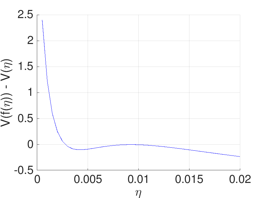
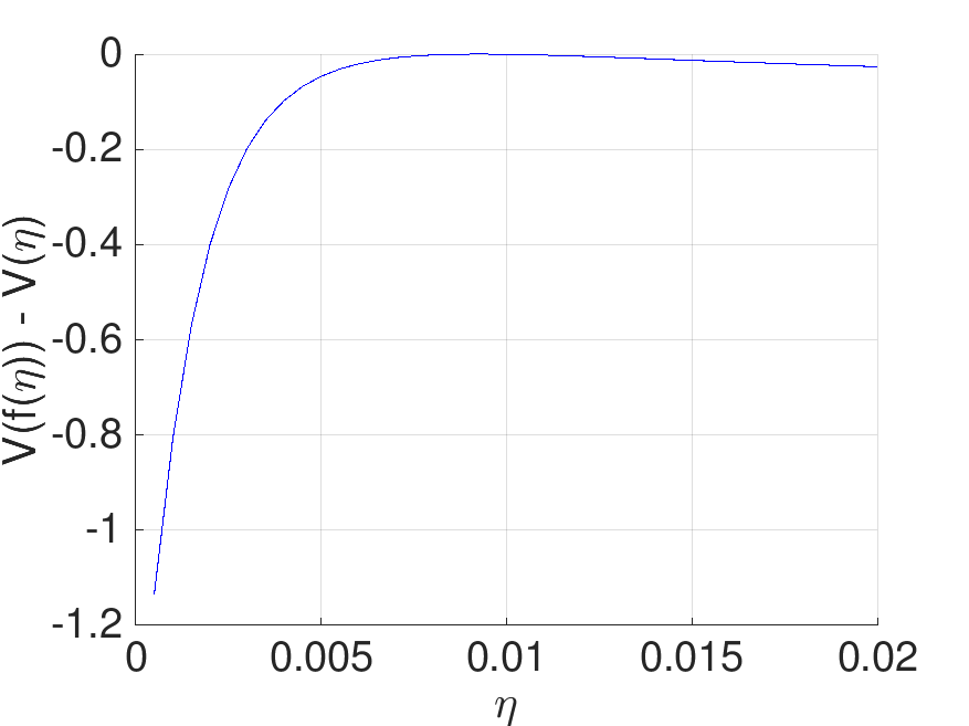
Figure 9. Behavior of Lyapunov Derivative with $\gamma=10^{-4}$ (Left) and $\gamma=10^{-5}$ (Right).

Again we consider the candidate Lyapunov function $V(\eta)=D(\eta)-D(\eta^{*})$. By discrete time Lyapunov function theory (Hahn, 1958), for global asymptotic stability, we require $\Delta V(\eta)=V(f(\eta))-V(\eta)<0,\forall\;\eta>0,\eta\neq\eta^{*}$. We evaluate $V(f(\eta))-V(\eta)$ with $V(\eta)=D(\eta)-D(\eta^{*})$ for the case when $k_{i}\leq 0.5$ as follows.

We plot $\Delta V(\eta)$ versus $\eta$ for a particular choice of parameters ($W=1,\gamma=10^{-4}\;\text{(Figure \ref{fig:globex}: Left) and}\;\gamma=10^{-5}\;\text{(Figure \ref{fig:globex}: Right)},B=100,k_{i}=0.5$). From the plot, it is clear that $\Delta V(\eta)\nless 0\;\forall\;\eta>0,\eta\neq\eta^{*}$ when $\gamma=10^{-4}.$ However, for sufficiently small $\gamma$ (say, $\gamma\leq 10^{-5}$) then $\Delta V(\eta)$ is sufficiently negative and (84) is globally asymptotically stable as depicted in Figure 9 (Right).

11.8. Proofs in Section 7

Lemma 0.

$\Delta V(\eta)$ is a decreasing function of $\eta$ for $\eta\in[0,\eta^{*}].$

Proof.

Consider the derivative of the function $\Delta V(\eta):$

(90) $$\Delta V^{\prime}(\eta)=\frac{-\frac{W\gamma}{\eta^{2}}\left(\frac{2W}{\eta}-B\right)}{1+\frac{\gamma}{\eta}\left(\frac{W}{\eta}-B\right)}$$

for $\eta<\eta^{*}$ we have

$$W/\eta-B>W/\eta^{*}-B=0$$

(91) $$\implies W/\eta-B>0\;\texttt{and}\;2W/\eta-B>0$$

Combining Equations (90) and (91) and considering $W,\eta,\gamma>0$ we have

$$\Delta V^{\prime}(\eta)<0$$

Hence $\Delta V(\eta)$ is a decreasing function of $\eta$ for $\eta\in[0,\eta^{*}].$

∎

Proof of Theorem 1

Proof.

Evaluating the function $\Delta V(\eta)$ at $\eta=\eta^{*}$ and setting $W/\eta^{*}=B$ we get

(92) $$\Delta V(\eta^{*})=-W\log\left[1+\frac{\gamma}{\eta^{*}}\bigg{(}\frac{W}{\eta^{*}}-B\bigg{)}\right]+B\gamma\left(\frac{W}{\eta^{*}}-B\right)=0$$

From Lemma 2 it is clear that $\Delta V(\eta)>\Delta V(\eta^{*})$ for all $\eta<\eta^{*}.$ Hence $\Delta V(\eta)>0$ for all $\eta<\eta^{*}.$

∎

11.9. Poisson Approximation for various distributions

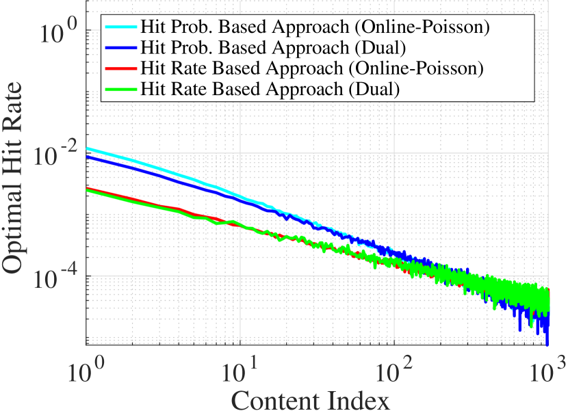
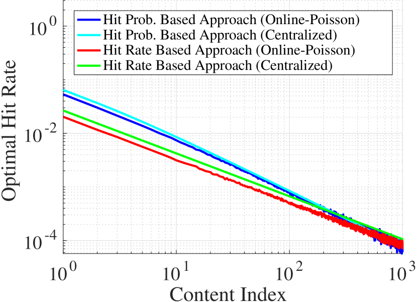
Figure 10. Poisson online approximation to Hyperexponential (Left) and weibull (Right) inter-requests.

11.9.1. Hyperexponential Distribution

W.l.o.g., we consider the arrivals follow a hyperexponential distribution with phase probabilities $p_{1i}=p_{2i}=0.5,$ and phase rate parameters $\theta_{1}$ and $\theta_{2}$ Zipf distributed with rates $0.4$ and $0.8,$ respectively. From Figure 5 (b), we can see that the optimal hit rates obtained through (38) exactly match those obtained from Dual under hyperexponential distribution by solving fixed point equation in (31). Similar performance was obtained for other parameters, especially for $p_{1i}\ll p_{2i}$, hence are omitted here.

11.9.2. Weibull Distribution

Similarly, we consider a Weibull distribution with shape parameter $k_{i}=0.5$. From Figure 5 (c), it is clear that this approximation is accurate. Note that when $k_{i}\rightarrow 1$, Weibull behaves more closed to exponential distribution, hence the accuracy of this approximation can be further improved. For smaller value of $k_{i},$ it has been shown that Weibull can be well approximated by hyperexponential distribution (Jin and Gonigunta, 2010). The performance of Poisson approximation to hyperexponential distribution has been discussed in Section 11.9.1.

11.10. Limiting Behavior of 2-MMPP

Case $1$: When $r_{1i}\rightarrow\infty$ and $r_{2i}\rightarrow\infty$, i.e., $x_{i}\rightarrow\infty$: From Equation (4), we get

$$u_{1i}=\frac{1}{2}\bigg{[}\theta_{1i}+\theta_{2i}+r_{1i}+r_{2i}-\sqrt{(\theta_{1i}-\theta_{2i}+r_{1i}-r_{2i})^{2}+4r_{1i}r_{2i}}\bigg{]}$$

$$=\frac{1}{2}\bigg{[}\frac{(\theta_{1i}+\theta_{2i}+r_{1i}+r_{2i})^{2}-(\theta_{1i}-\theta_{2i}+r_{1i}-r_{2i})^{2}-4r_{1i}r_{2i}}{\theta_{1i}+\theta_{2i}+r_{1i}+r_{2i}+\sqrt{(\theta_{1i}-\theta_{2i}+r_{1i}-r_{2i})^{2}+4r_{1i}r_{2i}}}\bigg{]}$$

(93) $$=\frac{2\theta_{1i}\theta_{2i}+2\theta_{1i}a_{2i}x_{i}+2\theta_{2i}a_{1i}x_{i}}{\theta_{1i}+\theta_{2i}+(a_{1i}+a_{2i})x_{i}+\sqrt{(\theta_{1i}-\theta_{2i}+(a_{1i}-a_{2i})x_{i})^{2}+4a_{1i}a_{2i}x_{i}^{2}}}.$$

When $x_{i}\rightarrow\infty$, by applying L’Hospital’s rule, we have

$$u_{1i}=\frac{2\theta_{1i}a_{2i}+2\theta_{2i}a_{1i}}{a_{1i}+a_{2i}+\lim\limits_{x_{i}\rightarrow\infty}\frac{(\theta_{1i}-\theta_{2i}+(a_{1i}-a_{2i})x_{i})(a_{1i}-a_{2i})+{4}a_{1i}a_{2i}x_{i}}{\sqrt{(\theta_{1i}-\theta_{2i}+(a_{1i}-a_{2i})x_{i})^{2}+4a_{1i}a_{2i}x_{i}^{2}}}}$$

$$={\frac{2\theta_{1i}a_{2i}+2\theta_{2i}a_{1i}}{a_{1i}+a_{2i}+\lim\limits_{x_{i}\rightarrow\infty}\frac{(\theta_{1i}-\theta_{2i})(a_{1i}-a_{2i})+(a_{1i}+a_{2i})^{2}x_{i}}{\sqrt{(\theta_{1i}-\theta_{2i})^{2}+2(\theta_{1i}-\theta_{2i})(a_{1i}-a_{2i})x_{i}+(a_{1i}+a_{2i})^{2}x_{i}^{2}}}}}$$

(94) $$={\frac{2\theta_{1i}a_{2i}+2\theta_{2i}a_{1i}}{a_{1i}+a_{2i}+\lim\limits_{x_{i}\rightarrow\infty}\frac{(a_{1i}+a_{2i})^{2}x_{i}}{(a_{1i}+a_{2i})x_{i}}}}={\frac{2\theta_{1i}a_{2i}+2\theta_{2i}a_{1i}}{a_{1i}+a_{2i}+a_{1i}+a_{2i}}}=\frac{\theta_{1i}a_{2i}+\theta_{2i}a_{1i}}{a_{1i}+a_{2i}}.$$

Similarly, we obtain $u_{2i}=\infty.$

Again, from Equation (4),

$$q_{1i} =\frac{\theta_{2i}^{2}r_{1i}+\theta_{1i}^{2}r_{2i}}{(\theta_{1i}r_{2i}+\theta_{2i}r_{1i})(u_{1i}-u_{2i})}-\frac{u_{2i}}{u_{1i}-u_{2i}}=\frac{\theta_{2i}^{2}a_{1i}+\theta_{1i}^{2}a_{2i}}{(\theta_{1i}a_{2i}+\theta_{2i}a_{1i})(-\delta)}+\frac{\theta_{1i}+\theta_{2i}+(a_{1i}+a_{2i})x_{i}}{2\delta}+\frac{1}{2}$$

(95) $$=\frac{(\theta_{1i}a_{2i}+\theta_{2i}a_{1i})(a_{1i}+a_{2i})x+\theta_{1i}\theta_{2i}(a_{1i}+a_{2i})-\theta_{1i}^{2}a_{2i}-\theta_{2i}^{2}a_{1i}}{2(\theta_{1i}a_{2i}+\theta_{2i}a_{1i})\sqrt{(\theta_{1i}-\theta_{2i}+(a_{1i}-a_{2i})x_{i})^{2}+4a_{1i}a_{2i}x_{i}^{2}}}+\frac{1}{2},$$

when $x_{i}\rightarrow\infty$, by applying L’Hospital’s rule, we have

$$q_{1i} =\frac{1}{2}+\frac{(\theta_{1i}a_{2i}+\theta_{2i}a_{1i})(a_{1i}+a_{2i})}{2(\theta_{1i}a_{2i}+\theta_{2i}a_{1i})\lim\limits_{x_{i}\rightarrow\infty}\frac{(\theta_{1i}-\theta_{2i}+(a_{1i}-a_{2i})x_{i})(a_{1i}-a_{2i})+4a_{1i}a_{2i}x_{i}}{\sqrt{(\theta_{1i}-\theta_{2i}+(a_{1i}-a_{2i})x_{i})^{2}+4a_{1i}a_{2i}x_{i}^{2}}}}$$

(96) $$=\frac{1}{2}+\frac{(\theta_{1i}a_{2i}+\theta_{2i}a_{1i})(a_{1i}+a_{2i})}{2(\theta_{1i}a_{2i}+\theta_{2i}a_{1i})(a_{1i}+a_{2i})}=\frac{1}{2}+\frac{1}{2}=1,$$

thus $q_{2i}=0.$

Case $2$: When $r_{1i}\rightarrow 0$ and $r_{2i}\rightarrow 0$, i.e., $x_{i}\rightarrow 0$: W.l.o.g., we assume $\theta_{1i}\geq\theta_{2i}.$ From Equation (4),

(97) $$\delta=\theta_{1i}-\theta_{2i},$$

then

(98) $$u_{1i}=\frac{1}{2}[\theta_{1i}+\theta_{2i}+(a_{1i}+a_{2i})x_{i}-\delta]=\theta_{2i},$$

similarly, we have $u_{2i}=\theta_{1i}.$

Again, from Equation (4), when $x_{i}\rightarrow 0,$ we obtain

$$q_{1i} =\frac{1}{2}+\frac{(\theta_{1i}a_{2i}+\theta_{2i}a_{1i})(a_{1i}+a_{2i})x+\theta_{1i}\theta_{2i}(a_{1i}+a_{2i})-\theta_{1i}^{2}a_{2i}-\theta_{2i}^{2}a_{1i}}{2(\theta_{1i}a_{2i}+\theta_{2i}a_{1i})\delta}$$

(99) $$=\frac{1}{2}+\frac{\theta_{1i}\theta_{2i}(a_{1i}+a_{2i})-\theta_{1i}^{2}a_{2i}-\theta_{2i}^{2}a_{1i}}{2(\theta_{1i}a_{2i}+\theta_{2i}a_{1i})(\theta_{1i}-\theta_{2i})}=\frac{\theta_{2i}a_{1i}}{\theta_{1i}a_{2i}+\theta_{2i}a_{1i}},$$

then $q_{2i}=\frac{\theta_{1i}a_{2i}}{\theta_{1i}a_{2i}+\theta_{2i}a_{1i}}.$

11.11. Limiting Behavior of m- state MMPP

In this section, we derive limiting behavior for an $m$- state MMPP arrival process.

Consider a $m$-state MMPP whose arrival rate is given by $\boldsymbol{\theta}[J(t)]$, where $J(t),t\geq 0$ is a $m$-state continuous-time Markov chain with generator $Q.$ Denote $\boldsymbol{r}=(r_{1},\cdots,r_{m}).$ Let $X_{k}$ be the time between the $(k-1)$-th and $k$-th arrivals with $X_{0}=0.$ When the Markov chain is in state $i$, arrivals occur according to a Poisson process with rate $\theta_{i}.$ Denote $\boldsymbol{\theta}=(\theta_{1},\cdots,\theta_{m}).$

Consider randomly chosen non-overlap time intervals $A_{1}=[a_{1},b_{1}],$ $A_{2}=[a_{2},b_{2}],$ $A_{3}=[a_{3},b_{3}],\cdots$ with $a_{1}<b_{1}<a_{2}<b_{2}<\cdots$. Let $A=(A_{1},A_{2},\cdots,A_{l}).$

11.11.1. The transition rate approaches zero

We first consider the case that the transition rate approaches zero, i.e., $\boldsymbol{r}\rightarrow\boldsymbol{0}$ ($r_{i}\rightarrow 0$ for $i=1,\cdots,m$).

Consider a time interval $[a,b]$ and $J(a)=i$ for $i=1,\cdots,m.$ Denote $M(a,b)$ be the number of state transition during $(a,b].$ For example, when $J(a)=i,$ $M_{i}(a,b)=0$ means all arrivals during $(a,b]$ follows the Poisson process with rate $\theta_{i}$.

We first show that when $\boldsymbol{r}\rightarrow\boldsymbol{0}$, the number of state transition approaches $0,$ i.e., $M(a,b)=0$ a.s.

Proposition 1.

Suppose $J(a)=i,$ then we have

(100) $$\mathbb{P}[J(b)=i,M(a,b)=0|J(a)=i]=e^{-r_{i}(b-a)}\rightarrow 1,\quad\text{as $\boldsymbol{r}\rightarrow\boldsymbol{0}$.}$$

Proof.

From the property of $m$-state MMPP, we directly have

$$\mathbb{P}[J(b) =i,M(a,b)=0|J(a)=i]=\mathbb{P}[M(a,b)=0|J(a)=i]=e^{-r_{i}(b-a)},$$

then take the limit as $\boldsymbol{r}\rightarrow\boldsymbol{0},$ which completes the proof. ∎

Then we immediately have

Corollary 0.

(101) $$\mathbb{P}[J(b)=i,M(a,b)>0|J(a)=i]\rightarrow 0,\quad\text{as $\boldsymbol{r}\rightarrow\boldsymbol{0}$.}$$

Proof.

$$\mathbb{P}[J(b)=i,M(a,b)>0|J(a)=i] \leq\mathbb{P}[M(a,b)>0|J(a)=i]$$

(102) $$=1-\mathbb{P}[M(a,b)=0|J(a)=i]=1-e^{-r_{i}(b-a)}\rightarrow 0,\quad{\text{as $\boldsymbol{r}\rightarrow\boldsymbol{0}.$ }}$$

Since $\mathbb{P}[J(b)=i,M(a,b)>0|J(a)=i]\geq 0,$ we have $\mathbb{P}[J(b)=i,M(a,b)>0|J(a)=i]\rightarrow 0$ as $\boldsymbol{r}\rightarrow\boldsymbol{0}.$ ∎

From Proposition 1 and Corollary 3, we also obtain

Proposition 2.

As $\boldsymbol{r}\rightarrow\boldsymbol{0},$ we have

(103) $$\mathbb{P}^{\boldsymbol{r}}[J(b)=j|J(a)=i]\rightarrow\delta_{ij},\quad\forall b>a,$$

where

$$\delta_{ij}=\begin{cases}1,\quad\text{if $i=j;$}\\ 0,\quad\text{otherwise.}\end{cases}$$

Proof.

Suppose $j\neq i,$ then

$$\mathbb{P}^{\boldsymbol{r}}[J(b)=j|J(a)=i] =1-\mathbb{P}^{\boldsymbol{r}}[J(b)=i|J(a)=i]$$

$$=1-\mathbb{P}^{\boldsymbol{r}}[J(b)=i,M(a,b)=0|J(a)=i]-\mathbb{P}^{\boldsymbol{r}}[J(b)=i,M(a,b)>0|J(a)=i]$$

(104) $$\stackrel{{\scriptstyle(a)}}{{\rightarrow}}0,\quad\text{as $\boldsymbol{r}\rightarrow\boldsymbol{0}$,}$$

where (a) holds from Proposition 1 and Corollary 3.

Hence, we have $\mathbb{P}^{\boldsymbol{r}}[J(b)=j|J(a)=i]=1$ for $j=i,$ which completes the proof. ∎

Then we immediately have

Corollary 0.

As $\boldsymbol{r}\rightarrow\boldsymbol{0},$ we have

(105) $$\mathbb{P}^{r}[J(a)=i]\rightarrow\mathbb{P}^{0}[J(a)=i]=1_{\{J(0)=i\}}.$$

Now we are ready to prove our main result. Our goal is to show that the interarrival times within one state is exponentially distributed as the transition rate approaches zero.

Proof for Theorem 1:

Proof.

Basically we need to show that

(106) $$\mathbb{P}^{\boldsymbol{r}}[A_{1},\cdots,A_{l}]\triangleq\mathbb{P}^{\boldsymbol{r}}[A]\rightarrow\mathbb{P}^{\boldsymbol{0}}[A]=\sum_{i}\mathbb{P}[J(0)=i]\prod_{j=1}^{l}\mathbb{P}^{0}[A_{j}|J(0)=i],\quad\text{as $\boldsymbol{r}\rightarrow\boldsymbol{0}$.}$$

First we consider the event $A_{1}=[a_{1},b_{1}]$. Denote $N(a_{1},b_{1})$ as the number of arrivals during interval $[a_{1},b_{1}].$ Then,

(107) $$\mathbb{P}^{\boldsymbol{r}}[N(a_{1},b_{1})=n_{1}]=\sum_{i}^{m}\mathbb{P}^{\boldsymbol{r}}[N(a_{1},b_{1})=n_{1}|J(a_{1})=i]\cdot\mathbb{P}^{\boldsymbol{r}}[J(a_{1})=i].$$

In the following, we characterize the two terms in the sum of (107), respectively.

On one hand, we have

$$\mathbb{P}^{\boldsymbol{r}}[N(a_{1},b_{1})=n_{1}|J(a_{1})=i] =\mathbb{P}^{\boldsymbol{r}}[N(a_{1},b_{1})=n_{1},M_{i}(a_{1},b_{1})=0|J(a_{1})=i]$$

$$+\mathbb{P}^{\boldsymbol{r}}[N(a_{1},b_{1})=n_{1},M_{i}(a_{1},b_{1})>0|J(a_{1})=i]$$

$$\stackrel{{\scriptstyle(a)}}{{=}}\mathbb{P}[N_{i}(a_{1},b_{1})=n_{1}]\cdot e^{-r_{i}(b_{1}-a_{1})}+o(1)$$

(108) $$=\mathbb{P}[N_{i}(a_{1},b_{1})=n_{1}],\quad\text{as $\boldsymbol{r}\rightarrow\boldsymbol{0}$},$$

where (a) holds from Proposition 1 and Corollary 3.

On the other hand, from Proposition 2, we have

(109) $$\mathbb{P}^{\boldsymbol{r}}[J(a_{1})=i]\rightarrow 1_{\{J(0)=i\}},\quad\text{as $\boldsymbol{r}\rightarrow\boldsymbol{0}.$}$$

Combing (11.11.1) and (109) into (107), we have

(110) $$\mathbb{P}^{\boldsymbol{r}}[N(a_{1},b_{1})=n_{1}|J(0)=i]\rightarrow\sum_{i}^{m}\mathbb{P}[N_{i}(a_{1},b_{1})=n_{1}],\quad\text{as $\boldsymbol{r}\rightarrow\boldsymbol{0}$.}$$

Given the arrivals of interval $[a_{1},b_{1}]$, we consider the second interval $[a_{2},b_{2}].$ From Proposition 2, as $\boldsymbol{r}\rightarrow\boldsymbol{0},$ we have

(111) $$\mathbb{P}(J(a_{2})=i|J(a_{1})=i)=1.$$

Therefore, following a similar argument, we have

(112) $$\mathbb{P}^{\boldsymbol{r}}[N(a_{2},b_{2}) =n_{2}|N(a_{1},b_{1})=n_{1},J(0)=i]=\sum_{i}^{m}\mathbb{P}[N_{i}(a_{2},b_{2})=n_{2}]\cdot 1_{\{J(0)=i\}},$$

and

$$\mathbb{P}^{\boldsymbol{r}}[N(a_{2},b_{2})=n_{2},N(a_{1},b_{1})=n_{1},J(0)=i]$$

$$= \mathbb{P}^{\boldsymbol{r}}[N(a_{2},b_{2})=n_{2}|N(a_{1},b_{1})=n_{1},J(0)=i]\cdot\mathbb{P}^{\boldsymbol{r}}[N(a_{1},b_{1})=n_{1}|J(0)=i]$$

(113) $$= \sum_{i}^{m}\mathbb{P}[N_{i}(a_{2},b_{2})=n_{2}]\cdot\sum_{i}^{m}\mathbb{P}[N_{i}(a_{1},b_{1})=n_{1}]$$

By induction, we have

$$\mathbb{P}^{\boldsymbol{r}}[N(a_{l},b_{l})=n_{l},\cdots N(a_{1},b_{1})=n_{1}|J(0)=i]$$

$$= \mathbb{P}^{\boldsymbol{r}}[N(a_{l},b_{l})=n_{l}|N(a_{l-1},b_{l-1})=n_{l-1},\cdots N(a_{1},b_{1})=n_{1},J(0)=i]$$

$$\cdots\cdot\mathbb{P}^{\boldsymbol{r}}[N(a_{2},b_{2})=n_{2}|N(a_{1},b_{1})=n_{1},J(0)=i]\cdot\mathbb{P}^{\boldsymbol{r}}[N(a_{1},b_{1})=n_{1}|J(0)=i]$$

(114) $$= \prod_{j=1}^{l}\sum_{i}^{m}\mathbb{P}[N_{i}(a_{j},b_{j})=n_{j}],$$

therefore,

(115) $$\mathbb{P}^{\boldsymbol{0}}[A_{1},\cdots,A_{l}]=\sum_{i}\mathbb{P}[J(0)=i]\prod_{j=1}^{l}\sum_{i}^{m}\mathbb{P}[N_{i}(a_{j},b_{j})=n_{j}]$$

which completes the proof. ∎

11.11.2. The transition rate approaches infinity

Now we consider the case that the transition rate approaches infinity, i.e., $\boldsymbol{r}\rightarrow\boldsymbol{\infty}$ ($r_{i}\rightarrow\infty$ for $i=1,\cdots,m$).

Proof for Theorem 2:

Proof.

W.l.o.g., consider a time interval $[a,b].$ Suppose that there are $k$ state transition occurs during $[a,b].$ As $\boldsymbol{r}\rightarrow\boldsymbol{\infty}$, we have $k\rightarrow\infty$ a.s.

For simplicity, we denote the length of each time interval within one state as $L_{j}$ for $j=1,\cdots,k$ and $\sum_{j}L_{j}=b-a.$ Then we have

(116) $$N(a,b)=\sum_{j}N_{j}(L_{j}),$$

where $N(a,b)$ is the number of arrivals in $(a,b]$ and $N_{j}(L_{j})$ is the number of arrivals during a time interval of length $L_{j}$ in $(a,b].$

W.l.o.g., suppose during the $j$-th interval, the MC is in state $i$ which has Poisson arrivals with rate $\theta_{i},$ for $i=1,\cdots,m.$ Let $L_{j}(i)$ be the length of the corresponding interval.

Consider any two time $t_{i}$ and $t_{i}^{\prime}$ with $t_{i}^{\prime}>t_{i}$ during which the MC is in state $i$ and $M_{i}(t_{i},t_{i}^{\prime})=0$. As $\boldsymbol{r}\rightarrow\infty,$ we have $|t_{i}^{\prime}-t_{i}|\rightarrow 0$ a.s..

Given the $m$-state MMPP with $\boldsymbol{r}\rightarrow\infty$ we have

(117) $$\mathbb{P}^{\boldsymbol{r}}(t_{i}^{\prime})=\mathbb{P}^{\boldsymbol{r}}(t_{i})e^{Q(t_{i}^{\prime}-t_{i})}=\mathbb{P}^{\boldsymbol{r}}(t_{i})e^{r^{\prime}Q_{0}(t_{i}^{\prime}-t_{i})},$$

where $r^{\prime}\rightarrow\infty$ is a scalar and $Q=r^{\prime}Q_{0}$.

The stochastic process described by (117) (call it Process $1$) is equivalent to a stochastic process with a finite-valued $Q_{0}$ (call it Process $2$) at stationary state (i.e., $t\rightarrow\infty$), since

(118) $$\mathbb{P}^{\boldsymbol{r}}(t_{i}^{\prime})\stackrel{{\scriptstyle(a)}}{{=}}\mathbb{P}^{\boldsymbol{r}}(t_{i})e^{r^{\prime}Q_{0}\cdot(t_{i}^{\prime}-t_{i})}\stackrel{{\scriptstyle(b)}}{{=}}\mathbb{P}^{\boldsymbol{r}}(t_{i})e^{Q_{0}\cdot r^{\prime}(t_{i}^{\prime}-t_{i})},$$

where (a) is from (117) and (b) is through reordered the elements. We have $r^{\prime}(t_{i}^{\prime}-t_{i})\rightarrow\infty$.

In other words,

• Process $1$: we consider a finite time interval $(a,b]$ with an infinite state transition rate $\boldsymbol{r}\rightarrow\infty$;

• Process $2$: we consider an infinite time interval $(ra,rb]$ with a finite state transition rate.

From (118), it is clear that Process $1$ and Process $2$ are equivalent.

Denote $\boldsymbol{\pi}=(\pi_{1},\cdots,\pi_{m})$ as the stationary distribution for the $m$-state MMPP. Then we have

(119) $$L_{j}(i)=\pi_{i}(b-a).$$

Since the stochastic process is in stationary at each interval for a particular state, and the arrivals in each state follows a Poisson process. Therefore, the interarrival times of the $m$-state MMPP are exponentially distributed since the mix of Poisson process is still Poisson. From (119), the equivalent arrival rate satisfies

(120) $$\bar{\theta}=\sum_{i}^{m}\theta_{i}\pi_{i}.$$

∎

References

• (1)
• Aven et al. (1987) O. I. Aven, E. G. Coffman, and Y. A. Kogan. 1987. Stochastic Analysis of Computer Storage. Springer Science & Business Media.
• Baccelli and Brémaud (2013) F. Baccelli and P. Brémaud. 2013. Elements of Queueing Theory: Palm Martingale Calculus and Stochastic Recurrences. Vol. 26. Springer Science & Business Media.
• Berger et al. (2014) D. Berger, P. Gland, S. Singla, and F. Ciucu. 2014. Exact Analysis of TTL Cache Networks. Performance Evaluation 79 (2014), 2–23.
• Boyd and Vandenberghe (2004) S Boyd and L Vandenberghe. 2004. Convex Optimization. Cambridge University Press.
• Cha et al. (2007) Meeyoung Cha, Haewoon Kwak, Pablo Rodriguez, Yong-Yeol Ahn, and Sue Moon. 2007. I Tube, You Tube, Everybody Tubes: Analyzing the World’s Largest User Generated Content Video System. In ACM IMC.
• Cha et al. (2009) Meeyoung Cha, Haewoon Kwak, Pablo Rodriguez, Yong-Yeol Ahn, and Sue Moon. 2009. Analyzing the Video Popularity Characteristics of Large-Scale User Generated Content Systems. IEEE/ACM Transactions on Networking 17, 5 (2009), 1357–1370.
• Che et al. (2002) H. Che, Y. Tung, and Z. Wang. 2002. Hierarchical Web Caching Systems: Modeling, Design and Experimental Results. IEEE Journal on Selected Areas in Communications 20, 7 (2002), 1305–1314.
• Dehghan et al. (2016) M. Dehghan, L. Massoulie, D. Towsley, D. Menasche, and YC Tay. 2016. A Utility Optimization Approach to Network Cache Design. In IEEE INFOCOM.
• Fagin (1977) Ronald Fagin. 1977. Asymptotic Miss Ratios over Independent References. J. Comput. System Sci. 14, 2 (1977), 222–250.
• Feldmann and Whitt (1997) A. Feldmann and W. Whitt. 1997. Fitting Mixtures of Exponentials to Long-Tail Distributions to Analyze Network Performance Models. In IEEE INFOCOM.
• Ferragut et al. (2016) Andrés Ferragut, Ismael Rodríguez, and Fernando Paganini. 2016. Optimizing TTL Caches under Heavy-tailed Demands. In ACM SIGMETRICS.
• Fofack et al. (2014a) N. C. Fofack, M. Dehghan, D. Towsley, M. Badov, and D. L. Goeckel. 2014a. On the Performance of General Cache Networks. In VALUETOOLS.
• Fofack et al. (2012) N. C. Fofack, P. Nain, G. Neglia, and D. Towsley. 2012. Analysis of TTL-based Cache Networks. In VALUETOOLS.
• Fofack et al. (2014b) N. C. Fofack, P. Nain, G. Neglia, and D. Towsley. 2014b. Performance Evaluation of Hierarchical TTL-based Cache Networks. Computer Networks (2014).
• Fricker et al. (2012) C. Fricker, P. Robert, J. Roberts, and N. Sbihi. 2012. Impact of Traffic Mix on Caching Performance in a Content-Centric Network. In INFOCOM WKSHPS.
• Garetto et al. (2016) M. Garetto, E. Leonardi, and v. Martina. 2016. A Unified Approach to the Performance Analysis of Caching Systems. ACM Transactions on Modeling and Performance Evaluation of Computing Systems 1, 3 (2016), 12.
• Gast and Van Houdt (2016) N. Gast and B. Van Houdt. 2016. Asymptotically Exact TTL-Approximations of the Cache Replacement Algorithms LRU(m) and h-LRU. In ITC 28.
• Hahn (1958) W. Hahn. 1958. Uber die Anwendung der Methode von Ljapunov auf Differenzen-gleichungen. Math. Ann. 136 (1958), 430–441.
• Jiang et al. (2017) B. Jiang, P. Nain, and D. Towsley. 2017. On the Convergence of the TTL Approximation for an LRU Cache under Independent Stationary Rrequest Processes. Arxiv preprint arXiv:1707.06204 (2017).
• Jin and Gonigunta (2010) T Jin and L.S. Gonigunta. 2010. Exponential Approximation to Weibull Renewal with Decreasing Failure Rate. J. Stat. Comput. Simul. 80, 3 (2010), 273–285.
• Jung et al. (2003) J. Jung, A. Berger, and H. Balakrishnan. 2003. Analysis of TTL-based Cache Networks. In IEEE INFOCOM.
• Kang and Sung (1995) S. Kang and D. Sung. 1995. Two-state MMPP Modelling of ATM Superposed Traffic Streams Based on The Characterisation of Correlated Interarrival Times. In IEEE GLOBECOM.
• Kelly (1997) Frank Kelly. 1997. Charging and Rate Control for Elastic Traffic. Transactions on Emerging Telecommunications Technologies 8, 1 (1997), 33–37.
• Kelly et al. (1998) F. P. Kelly, A. K. Maulloo, and D. K.H. Tan. 1998. Rate Control for Communication Networks: Shadow Prices, Proportional Fairness and Stability. Journal of the Operational Research society 49, 3 (1998), 237–252.
• Li et al. (2018) J. Li, S. Shakkottai, J. C. S. Lui, and V. Subramanian. 2018. Accurate Learning or Fast Mixing? Dynamic Adaptability of Caching Algorithms. IEEE Journal on Selected Areas in Communications (2018).
• Ma and Towsley (2015) R.T. Ma and D. Towsley. 2015. Cashing in on Caching: On-demand Contract Design with Linear Pricing. In CoNext.
• Meyn and Tweedie (2009) Sean P Meyn and Richard L Tweedie. 2009. Markov Chains and Stochastic Stability. Cambridge University Press.
• Panigrahy et al. (2017a) N. K. Panigrahy, J. Li, and D. Towsley. 2017a. Hit Rate vs. Hit Probability Based Cache Utility Maximization. In ACM MAMA.
• Panigrahy et al. (2017b) N. K. Panigrahy, J. Li, F. Zafari, D. Towsley, and P. Yu. 2017b. Optimizing Timer-based Policies for General Cache Networks. Arxiv preprint arXiv:1711.03941 (2017).
• Paxson and Floyd (1995) Vern Paxson and Sally Floyd. 1995. Wide-Area Traffic: The Failure of Poisson Modeling. IEEE/ACM Transactions on Networking 3, 3 (1995), 226–244.
• Rodriguez et al. (2001) P. Rodriguez, C. Spanner, and E. W. Biersack. 2001. Analysis of Web Caching Architectures: Hierarchical and Distributed Caching. IEEE/ACM Transactions on Networking (2001).
• Smith and Coit (1996) Alice E Smith and David W Coit. 1996. Evolutionary Computation. Institute of Physics Publishing and Cambridge University Press.
• Srikant and Ying (2013) R. Srikant and Lei Ying. 2013. Communication Networks: an Optimization, Control, and Stochastic Networks Perspective. Cambridge University Press.
• Weinberg (2016) G.V. Weinberg. 2016. Kullback Leibler Divergence and the Pareto Exponential Approximation. SpringerPlus 5 (2016).
• Zerfos et al. (2013) P. Zerfos, M. Srivatsa, H. Yu, D. Dennerline, H. Franke, and D. Agrawal. 2013. Platform and Applications for Massive-scale Streaming Network Analytics. IBM Journal for Research and Development: Special Edition on Massive Scale Analytics 57, 136 (2013), 1–11.
• Zink et al. (2008) M. Zink, K. Suh, Y. Gu, and J. Kurose. 2008. Watch Global, Cache Local: YouTube Network Traffic at a Campus Network: Measurements and Implications. In Electronic Imaging.