Electrical spin manipulation in graphene nanostructures

Abstract

We propose a mechanism to drive singlet-triplet spin transitions, electrically, in a wide class of graphene nanostructures that present pairs of in-gap zero modes, localized at opposite sublattices. Examples are rectangular nanographenes with short zigzag edges, armchair ribbon heterojunctions with topological in-gap states and graphene islands with sp³ functionalization. The interplay between the hybridization of zero modes and Coulomb repulsion leads to symmetric exchange interaction that favors a singlet ground state. Application of an off-plane electric field to the graphene nanostructure generates an additional Rashba spin-orbit coupling, which results in antisymmetric exchange interaction that mixes $S=0$ and $S=1$ manifolds. We show that modulation in time of either the off-plane electric field or the applied magnetic field permits to perform electrically driven spin resonance in a system with very long spin relaxation times.

Spin $1/2$ systems provide the simplest physical realization of a quantum bitNielsen and Chuang (2002); Ardavan and Briggs (2011). Unsurprisingly, localized spins, both electronicKane (1998); Loss and DiVincenzo (1998); Burkard et al. (1999) and nuclearGershenfeld and Chuang (1997), were early on proposed as physical platforms to store and manipulate quantum information taking advantage from the enormous know-how in magnetic resonance techniques. In spite of several remarkable experimental breakthroughs, using both phosphorous donors in SiliconMuhonen et al. (2014) as well as III-V semiconductor quantum dotsElzerman et al. (2004); Koppens et al. (2005), the fabrication of spin based quantum computer in solid state platforms, going beyond a few quantum bits, remains a daunting challenge. One of the main problems is the upper limit for spin coherence lifetimes $T_{2}$ due to hyperfine coupling to the nuclear spins Khaetskii et al. (2002).

Strategies to mitigate this problem come from two fronts. First, using materials with a small, or even null, density of nuclear spins, such as grapheneTrauzettel et al. (2007) and carbon nanotube based quantum dotsLaird et al. (2013) or isotopically pure siliconSteger et al. (2012). Second, using a different degree of freedom to store quantum information, such as the singlet-triplet $S_{z}=0$ states that arise for pairs of exchange coupled spinsPetta et al. (2005). However, this approach requires the use of 2 electron spins per qubit, with the resulting fabrication overhead.

Interestingly, a class of graphene nanostructures that can be synthesized with bottom-up techniquesWang et al. (2016, 2017) provide naturally, without the need of electrical control of the number of carriers, exchange coupled unpaired spin electron duets in an environment with a low density of carbon nuclear spins. In figure 1 we show three such graphene nanostructures: graphene rectangular ribbons with short zigzag edges (in the following ribbons), armchair ribbon heterojunctions with topological in-gap states (in the following heterojunctions) and $sp^{3}$ functionalized graphene. These three systems form a class with the following common properties:

1. On account of their finite size, they have a gapped spectrum, except for two single-particle in-gap states, that we label $\psi_{\pm}$, and host two electrons (see figure 2(b)).

2. The wave function of these in-gap states turns out to be a linear combination of two zero mode states that are mostly localized in one of the sublattices, labeled $A$ and $B$ that form the honeycomb lattice (figure 2(d, e, f, g)). We refer to these zero mode states as $\psi_{A}$ and $\psi_{B}$.

3. The overlap of $\psi_{A}$ and $\psi_{B}$, and thereby the bonding-antibonding splitting ($\delta\equiv\epsilon_{+}-\epsilon_{-}$) of the single-particle spectrum, depends on the geometrical properties of the graphene structure, and is therefore an important design parameter (figure 2(c)).

4. The electronic ground state is a singlet with $S=0$, the first excited state is a triplet $S=1$ and their energy separation $J$ is proportional to $\delta^{2}/\tilde{U}$, where $\tilde{U}$ is the Coulomb energy overhead of adding a second electron in the localized states ($\psi_{A,B}$).

In this work two things are done. First, we provide a quantum theory, beyond mean field approximation, for the spin states and the exchange $J$ in this class of graphene nanostructures. Second, we study how the application of an off-plane electric field generates a Dzyaloshinsky-Moriya (DM) antisymmetric exchangeDzyaloshinsky (1958); Moriya (1960) that could be used to enable spin-transitions between the ground state singlet and the states in the triplet. Importantly, these transitions are strictly forbidden, in the absence of DM interaction, in conventional electron-paramagnetic resonance experiments, where both spins interact with a dc field $B_{0}$ and a perpendicular $ac$ field $B_{ac}$ and only transitions that conserve $S$ may be induced. Therefore, our results pave the way towards electrically driven spin resonance in graphene nanostructures, complementing recent experiments on electrically detected spin resonance in grapheneMani et al. (2012); Lyon et al. (2017).

Graphene zero modes with a wave function localized in a single sublattice were predicted to occur in zigzag graphene edgesNakada et al. (1996); Fujita et al. (1996) and around carbon atoms with sp³ functionalization Wehling et al. (2007); Yazyev and Helm (2007a); Pereira et al. (2008); Palacios et al. (2008a). Their direct experimental observation, by means of scanning tunneling microscopy, has been reported both for the edge states of rectangular nanographenes with short zigzag edges Wang et al. (2016) as well as for individual and for pairs of chemisorbed hydrogen atoms in grapheneUgeda et al. (2010); González-Herrero et al. (2016). These sub-lattice polarized zero modes are expected to host unpaired spin electrons, giving rise to the formation of local moments Fujita et al. (1996); Son et al. (2006a, b); Kumazaki and S. Hirashima (2007); Fernández-Rossier and Palacios (2007); Fernández-Rossier (2008); Palacios et al. (2008a); Yazyev (2010); Lado and Fernández-Rossier (2014); García-Martínez et al. (2017). Sublattice polarized zero modes have recently been predicted Cao et al. (2017) to exist as in-gap topological states at the interface of certain graphene ribbons with armchair edges, shown in figure 1(b). Recent progress in fabrication of graphene ribbon heterojunctionsRuffieux et al. (2016); Wang et al. (2017) shows that fabrication of this type of structure is not out of reach of state of the art in nanographene synthesis.

The exploration with STM of some of the graphene nanostructures studied here has been demonstratedGonzález-Herrero et al. (2016); Wang et al. (2016, 2017). With this approach, the application of an off-plane electric field significantly larger than in conventional field effect transistor geometries is possible. On the other hand, STM can be used to carry out electrically driven spin paramagnetic resonance of individual atoms Baumann et al. (2015); Choi et al. (2017); Natterer et al. (2017) and coupled spin $1/2$ atoms Yang et al. (2017). Therefore, the electrical manipulation of localized spin states in graphene seems within reach with state of the art surface scanning probes.

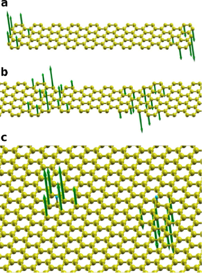
Figure 1: Three types of graphene nanostructures that host pairs of zero modes localized in opposite sublattices. $a)$ Rectangular graphene nanoribbons with short zigzag edges that host 1 unpaired electron each. $b)$ Armchair graphene heterojunctions, hosting 1 zero mode at each interface Cao et al. (2017). $c)$ Graphene nanoisland with sp³ functionalization (chemisorbed atomic hydrogen). In the three cases, the green arrows represent the magnetization calculated with a mean field Hubbard model.

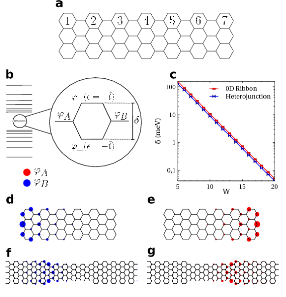
Figure 2: $a)$ Graphene nanoribbon with $W=7$. $b)$ Sketch of the single-particle energy spectrum for the graphene nanostructures shown in figure 1. A gap, separating the doubly occupied states from the empty states, contains 2 in-gap states, $\epsilon_{\pm}$, split by $\delta=\epsilon_{+}-\epsilon_{-}$. $c)$ Dependence of $\delta$ on the distance between both for edge and interface states. The splitting arises from the hybridization of the zero modes, $\psi_{A}$ and $\psi_{B}$, for the ribbons (d, e) and heterojunctions (f, g) (see equation (2)).

Modeling. We model the single particle states of the graphene nanostructures both with the standard one-orbital tight-binding model, with first neighbor hopping $t=2.7$ eV. Electron-electron interactions are treated with the Hubbard model, both at the mean field approximation, including all the single particle states, or exactly for the subspace of 2 electrons and 2 orbitals that controls the spin properties of the studied systems. In the case of graphene nanostructures, it is well known that mean field Hubbard model calculations and density functional calculations give very similar resultsFernández-Rossier and Palacios (2007); Ortiz et al. (2016). The spin orbit coupling effect considered in the following will be of Rashba type,Kane and Mele (2005); Min et al. (2006); Konschuh et al. (2010) that can be externally modulated with an electric field.

The non-interacting spectrum. A scheme of the single-particle spectrum characteristic of the gapped graphene with 2 in-gap states is shown in figure 2(b). The energies and wave-functions of the in-gap states are denoted by $\epsilon_{\pm}$ and $\psi_{\pm}$ respectively. It is always possibleSoriano and Fernández-Rossier (2012) to write down the wave function of a couple of conjugate states, with single-particle energy $E$ and $-E$, in terms of the same sublattice polarized states $\psi_{A}$ and $\psi_{B}$. Therefore, we write

$$\psi_{A}(i)\equiv\frac{1}{\sqrt{2}}\left(\psi_{+}(i)+\psi_{-}(i)\right)$$

$$\psi_{B}(i)\equiv\frac{1}{\sqrt{2}}\left(\psi_{+}(i)-\psi_{-}(i)\right)$$ (1)

In the case of the in-gap states, the peculiar property of the resulting $\psi_{A}$ and $\psi_{B}$ is that they are spatially separated. As a result, the resulting splitting that arises from the hybridization of the zero modes,

$$\delta=2\langle\psi_{A}|{\cal H}_{0}|\psi_{B}\rangle\equiv 2\tilde{t}$$ (2)

turns out to be small. In figure 2(c) we plot $\delta$ for different nanographenes as a function of the spatial separation between the zero modes. It is apparent and well knownNakada et al. (1996) that this quantity decays exponentially with $W$. In the limit where $W$ is very large (see figure 2(c)), $\delta$ vanishes, and the energy of the in-gap states goes to $E=0$, showing that these sublattice polarized states are zero modes.Nakada et al. (1996)

Our next task is to demonstrate that in-gap states in these structures hold local moments. This has been established, using either DFT and/or mean field Hubbard model calculations, in the case of infinitely long graphene ribbons with zigzag edgesFujita et al. (1996); Fernández-Rossier (2008), as well as the small nanoribbons considered hereRuffieux et al. (2016); Wang et al. (2017), and also for hydrogenated grapheneYazyev and Helm (2007b); Soriano et al. (2010); González-Herrero et al. (2016); García-Martínez et al. (2017). To the best of our knowledge, the emergence of local moments in the case of un-doped topological junctions has not been explored yet. We therefore carry out a mean field Hubbard model calculation (see supplementary material for details) to address the emergence of local moments associated to the topological in-gap states and, for comparison, the well understood case of graphene nanoribbons. For the topological in-gap states, we consider a structure with periodic boundary conditions and two interfaces, that accommodate one in-gap state each. For $U=t=2.7.eV$, we find broken symmetry solutions with a finite local magnetization, $M(i)=\langle S_{z}(i)\rangle$ that is mostly located in the region where either $\psi_{A}$ or $\psi_{B}$ are non-zero, for all structures except those where $\delta$ is large (i.e., those where $\psi_{A}$ and $\psi_{B}$ are strongly hybridized). This applies both for heterojunctions and nanoribbons. In the mean field approximation, the transition between non-magnetic and broken symmetry transitions is abrupt. The mean field broken symmetry solutions have lower energy for antiferromagnetic (AF) correlations between spins in opposite sublattice, that result in a total zero magnetic moment $\sum_{i}M(i)=0$ (see figure 1(b)). Solutions with a net magnetic moment and ferromagnetic (FM) correlations between opposite sublattices have higher energy and $\sum_{i}M(i)=1$, as expected for as expected for a $S=1$ configuration in two antiferromagnetically coupled $S=1/2$.

We study the exchange energy as the difference between FM and AF solutions $J_{MF}=E_{FM}-E_{AF}$ for several different nanographenes, both for the edge and interface states. We find that, for the same value of $W$, the exchange is larger for ribbons than heterojunctions. This ultimately arises from the larger hybridization of the edge zero modes, compared with the topological interface zero modes (see figure 2(c)). We show in figure 3 that $J_{MF}$ can be as large as 40 meV for graphene ribbons, and be made as small as necessary by increasing the distance $W$ between the zero modes. Importantly, as we show in figure 3(b), we find that, both for ribbons and heterojunctions, exchange energy scales as

$$J_{MF}\propto\frac{\tilde{t}^{2}}{\tilde{U}}$$ (3)

where

$$\tilde{U}=U\sum_{i}|\psi_{A}(i)|^{4}=U\sum_{i}|\psi_{B}(i)|^{4}=U\eta$$ (4)

is the average addition energy for these states, as computed in the Hubbard model (see supplementary material) and $\eta$ is the inverse participation ratio of the zero mode states. This scaling provides a strong indication that the mechanism of antiferromagnetic interaction is kinetic exchangeAnderson (1959); Moriya (1960), that arises naturally for half-filled Hubbard dimers. Our calculations show that, for a given type of structures (ribbon or heterojunction), the inverse participation ratio $\eta$ is quite independent of $W$. Thus, for the zigzag edge zero modes we find $\eta\approx 0.1$ and for the topological in-gap states we find $\eta\approx 0.035$. The smaller $\eta$ for the heterojunction states can be anticipated, as they can spread at both sides of the junction, in contrast with the edge states.

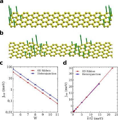
Figure 3: $a)$, $b)$ Magnetization in the ferromagnetically aligned (FM) configuration , as calculated within the mean field approximation for graphene ribbon. $c)$ Dependence of the exchange energy, calculated within the mean field Hubbard model, $J=E_{FM}-E_{AF}$ on the dimensions of the graphene nanostructure and $d)$ scaling of $J$ with $\frac{\tilde{t}^{2}}{\tilde{U}}$, demonstrating kinetic exchange.

All these results, most notably the scaling of equation 3, strongly suggest that magnetic correlations are governed by the two electrons that occupy the two in-gap states. This is also the case for graphene ribbons with infinitely long zigzag edges Fernández-Rossier (2008). In order to go beyond the mean field picture and to be able to describe local moments in these nanographenes with a full quantum theory without breaking symmetry, we restrict the Hilbert space to the configurations of 2 electrons in the two zero modes. To do so, we represent the Hubbard interaction in the one body basis defined by the states $\psi_{A}$ and $\psi_{B}$. The Hamiltonian so obtained is a two site Hubbard model with renormalized hopping and on-site energy:

$${\cal H}_{\rm eff}=\tilde{t}\sum_{\sigma}\left(a^{\dagger}_{\sigma}b_{\sigma}+b^{\dagger}_{\sigma}a_{\sigma}\right)+\tilde{U}\left(n_{A\uparrow}n_{A\downarrow}+n_{B\uparrow}n_{B\downarrow}\right)$$ (5)

where $a^{\dagger}_{\sigma}=\sum_{i}\psi_{A}(i)c^{\dagger}_{i\sigma}$ and $b^{\dagger}_{\sigma}=\sum_{i}\psi_{B}(i)c^{\dagger}_{i\sigma}$ are the operators that create an electron in the zero modes $\psi_{A}$ and $\psi_{B}$ with spin $\sigma$, respectively. In turn, $n_{A,\sigma}=a^{\dagger}_{\sigma}a_{\sigma}$ is the number operator for the $\psi_{A}$ state with spin $\sigma$. In addition, we consider the Zeeman coupling to a magnetic field,

$${\cal H}_{\rm Z}=g\mu_{B}\sum_{\sigma,\sigma^{\prime}}\vec{B}\cdot\vec{S}_{\sigma,\sigma^{\prime}}\left(a^{\dagger}_{\sigma}a_{\sigma^{\prime}}+b^{\dagger}_{\sigma}b_{\sigma^{\prime}}\right)$$ (6)

where $\vec{S}_{\sigma,\sigma^{\prime}}$ are the $S=1/2$ spin matrices, $g=2$ is the gyromagnetic factor and $\mu_{B}=57\mu\,eV\,T^{-1}$ is the Bohr magneton.

Hamiltonian (5) is a two-site Hubbard model, where the sites correspond to the zero mode states $\psi_{A,B}$, shown in figure 2(b, c, d, e). This model can be solved analyticallyJafari (2008) or by a straight-forward numerical diagonalization (see supplementary material). For the relevant case of 2 electrons, the dimension of the Hilbert space is 6 and the ground state is always a singlet. We are interested in the limit $\tilde{t}<<\tilde{U}$. A cartoon of the spectrum is shown in figure 4(a). In that case the excited state manifold is a triplet, way below two excited singlets that describe states with double occupation of the zero modes.

Unlike the mean field solution, the exact solution of Hamiltonian (5) has no abrupt change of behavior from non-magnetic to magnetic solutions. However, depending on the ratio $\frac{\tilde{t}}{\tilde{U}}$, the physical properties of the system are very different. This is quantified by the weight on the ground state wave function of the states where 2 electrons occupy one zero mode, denoted by $P_{2}$. For $U=0$ the ground state is a trivial singlet, formed by two electrons in the lowest energy in-gap state and $P_{2}=0.5$. For very small $\hat{t}/\hat{U}$, $P_{2}$ goes to zero. For a fixed value of $t$ and $U$, the effective hopping $\tilde{t}$ is controlled by the dimensions of the nanographene structure. Thus, in figure 5(a), we show $P_{2}$ for a nanoribbon, assuming $U=t$, as a function of the ribbon width $W$. We see that for $W>9$, the weight of the double occupancy configurations is smaller than 5 percent of the state, and the charge fluctuations are effectively frozen. In that limit, it is well knownAnderson (1959); Moriya (1960) that the four lowest levels in the model of equation (5) can be mapped into the Heisenberg Hamiltonian:

$${\cal H}_{\rm Heis}=J_{H}\vec{S}_{A}\cdot\vec{S}_{B}$$ (7)

where $\vec{S}_{A,B}$ are the spin $\frac{1}{2}$ operators describing the electronic spins localized in states $\psi_{A}$ and $\psi_{B}$, respectively and $J_{H}\simeq\frac{4\tilde{t}^{2}}{\tilde{U}}$. The Hamiltonian of equation (7) has a ground state singlet ($S=0$)and an excited state triplet with $S=1$, separated in energy by $\Delta=E(S=1)-E(S=0)=J_{H}$ (see figure 4(b)). heterojunctions. Effectively, the upper limit to $J_{H}$ is marked by the crossover to the un-correlated regime, where double occupancy $P_{2}$ is not negligible. On the other side, $J$ can be made exponentially small when the distance between the two zero modes is increased.

We now consider the effect of spin-orbit interactions induced by an off-plane electric field, $\vec{E}$, on the spin dynamics of these 4 states. These can be described with a Rashba spin-orbit couplingKane and Mele (2005); Min et al. (2006); Konschuh et al. (2010),

$${\cal H}_{\rm R}=it_{R}\sum_{\sigma,\sigma^{\prime},\langle i,j\rangle}\vec{E}\cdot\left(\vec{d}_{i,j}\times\vec{\sigma}_{\sigma,\sigma^{\prime}}\right)c^{\dagger}_{i\sigma}c_{j\sigma^{\prime}}$$ (8)

where $\langle i,j\rangle$ labels first neighbors and $\vec{d}_{ij}$ in the vector linking them. $\sigma=\pm$ labels the eigenstates of the spin matrix $S_{z}=\frac{1}{2}\sigma_{z}$, $\vec{\sigma}_{\sigma,\sigma^{\prime}}$ are the Pauli matrices (with eigenvalues $\pm 1$), and the $c$ and $c^{\dagger}$ are second quantization fermionic operators. The extrinsic spin-orbit coupling constant $t_{R}$ is zero unless an off-plane electric field is applied $E_{0}\hat{z}$ to break mirror symmetry Min et al. (2006):

$$t_{R}=\frac{eEz_{0}}{9V_{sp\sigma}}\xi$$ (9)

where $e$ is the electron charge, $Ez_{0}$ is the voltage drop across atomically thin grapheneMin et al. (2006), $\xi=6meV$ is the spin orbit coupling of carbon and $V_{sp\sigma}$ is the hybridization between $p$ and $s$ orbitals.

For an electric field $E=50{\rm Volt}/300nm$, standard for graphene field effect transistorsNovoselov et al. (2004), we have $t_{R}\simeq 3.7\mu$eV. Importantly, with an STM tip it is possible to apply a few volts at 1 nm, so that $t_{R}=100\mu$eV could be reached.

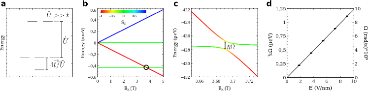
Figure 4: $a)$ Scheme of energy levels for 2 site Hubbard model with 2 electrons. $b)$ Evolution of 4 lowest energy eigenstates of equation (5), including the Zeeman (equation (6)) for the ribbon with $W=10$, $U=t$ and Rashba, for $E=10\ V/nm$. The effect of the Rashba interaction is only apparent in the anticrossing of the $S_{z}=-1$ and $S=0$ states, shown in the inset. $c)$ Zoom of the anticrossing. $d)$ Magnitude of the singlet-triplet anticrossing energy $\hbar\Omega$ as a function of the electric field.

The Rashba spin-orbit Hamiltonian adds an spin-flip hopping in the 2-site model (5):

$${\cal V}_{\rm R}=\sum_{\sigma}\left(\tilde{t}_{R}(\sigma)a^{\dagger}_{\sigma}b_{\overline{\sigma}}+\tilde{t}_{R}(\sigma)^{*}b^{\dagger}_{\overline{\sigma}}a_{\sigma}\right)$$ (10)

where $\overline{\sigma}=-\sigma$ and

$$\tilde{t}_{R}(\sigma)=\sigma\langle\psi_{A\sigma}|{\cal V}_{\rm R}|\psi_{B\overline{\sigma}}\rangle\equiv\sigma\tilde{t}_{R}$$ (11)

For the graphene nanostructures considered here, we find that $\tilde{t}_{R}$ is real. Unexpectedly, we find that $\frac{\tilde{t}_{R}}{\tilde{t}}$ is always more than 5 times larger than $\frac{t_{R}}{t}$. The origin of the enhancement of the Rashba interaction in graphene nanostructures has to do with a constructive interference between the modulation of the sign of the in-gap zero modes states and the angle-dependence sign of the Rashba hopping.

The addition of this spin-flip hopping to the Hubbard model results, in the strong coupling limit $\tilde{U}>>\tilde{t}$, in two types of additional terms to the effective spin HamiltonianMoriya (1960); Goth and Assaad (2014):

$${\cal V}_{\rm DM}=J_{\rm DM}\left[\left(S_{A}^{x}S_{B}^{z}-S_{A}^{z}S_{B}^{x}\right)+\left(S_{A}^{z}S_{B}^{y}-S_{A}^{y}S_{B}^{z}\right)\right]$$ (12)

$${\cal V}_{\rm anis}=J_{z}S_{A}^{z}S_{B}^{z}$$ (13)

with $J_{DM}=\frac{8\tilde{t}\tilde{t}_{R}}{\tilde{U}}$ and $J_{z}=4\frac{\tilde{t}^{2}-\tilde{t}_{R}^{2}}{\tilde{U}}$.

The first term (equation 12) is the widely studied anisotropic exchange postulated by Dzyaloshinsky Dzyaloshinsky (1958) and derived by MoriyaMoriya (1960). It does not conserve $S_{z}$. The physical origin is transparent: exchange arises from the virtual hopping of one electron between states $\psi_{A}$ and $\psi_{B}$. This hopping occurs through a spin conserving channel, with amplitude $\tilde{t}$ and through a spin-flip channel $\tilde{t}_{R}$. Thus, two hoppings through the same channel, either spin conserving or spin flip, preserve the spin of the electron. In contrast, the crossed term, by which only one hopping preserves the spin, results in an effective interaction that does not conserve $S_{z}$. This is the DM interaction, which is the dominant addition coming from the Rashba perturbation, given that $\tilde{t}>>\tilde{t}_{R}$.

The DM interaction scales with the kinetic exchange as $J_{\rm DM}=\frac{\tilde{t}_{R}}{\tilde{t}}J$. Thus, $J$ is in the range of meV, so that $J_{\rm DM}$ in this system is, at most, in the $\mu$eV. Whereas this is a small energy scale, it has a qualitatively important consequence: it permits otherwise forbidden transitions between singlet and triplet manifolds. This is shown in figure 4(b), where we plot the spectrum of the 2-site Hubbard model, as a function of the off-plane magnetic field $B$, for a ribbon with $W=10$, chosen so that for a moderate magnetic field the Zeeman splitting of the triplet manifold offsets the singlet-triplet splitting $J$. The calculation is done including the effect of the Rashba interaction. The effect of the small Rashba interaction is only apparent when the $S_{z}=-1$ triplet state gets close in energy to the $S=0$ ground state. In the absence of Rashba interaction, these two spectral lines would cross each other.

We have verified that dipolar interactions (see supplementary material C) are small (for the $W=10$ nanoribbon, $10^{-2}\mu$eV ). Importantly, they produce an anisotropic symmetric exchange that does not couple $S=0$ with the $S_{z}=\pm 1$ states. In addition, dipole interaction can not be modulated electrically in this class of systems.

The states $S_{z}=-1$ from the triplet and the $S=0$ define a two level system with Hamiltonian:

$${\cal H}_{\rm TLS}=\frac{1}{2}\hbar\omega_{0}\left(\tau_{z}+1\right)+\frac{\hbar}{2}\Omega\tau_{x}$$ (14)

where $\tau_{z}$ and $\tau_{x}$ are the $S=1/2$ Pauli matrices (with eigenvalues $\pm 1$), $\hbar\omega_{0}=J-g\mu_{B}B$ is the splitting of the two levels when the electric field is zero, and

$$\hbar\Omega\propto\frac{\tilde{t}}{\tilde{U}}\tilde{t}_{R}$$ (15)

is the Rabi coupling. As expected from equations (9, 10, 11 and 15) , we find that $\hbar\Omega$ scales linearly with the electric field (figure 4(d)). It must be noted that our TLS is different from the case of singlet-triplet qubits where both states have $S_{z}=0$. As a result, the energy difference can be tuned with a magnetic field, but this also removes the protection against fluctuations of the magnitude of the external magnetic field that makes singlet-triplet qubits convenientKoppens et al. (2005).

The energy scale $\hbar\Omega$ defines a Rabi coupling between the spin split levels. In order to asses its magnitude, we first compare it with the Rabi coupling achieved by pumping a spin $S=1/2$ system with the ac magnetic field of a microwave. The magnetic field of a microwave generated in pulsed state of the art ESR setup is, at most, $B_{ac}=4$mT, leading to a Rabi splitting of $g\mu_{B}B_{ac}\simeq 0.4\mu$eV. Thus, electrical driving can overcome conventional microwave coupling, showing that it can be used to efficiently drive singlet-triplet spin transitions in graphene nanostructures.

In order to assess the strength of the system response to the electrically driven spin resonance, it is important to compare the Rabi coupling, that drives the TLS out of equilibrium, with the spin relaxation $T_{1}$ and decoherence $T_{2}$ times. For instance, the steady state solution of the Bloch equation for a TLS driven with a resonant $ac$ Rabi coupling is fully determined by the dimensionless constant $x=\Omega^{2}T_{1}T_{2}$ (see supplementary material). Both $T_{1}$ and $T_{2}$ depend a lot on whether the nanographenes are deposited on top of a conductor or an insulator. In the former case, exchange interaction with the electrons in the conductor will be the dominant spin relaxation and decoherence mechanismDelgado and Fernández-Rossier (2017).

We now provide a rough estimate of the contribution to $T_{2}$ coming from an intrinsic mechanism, namely, the hyperfine coupling with the nuclear spins of the hydrogen atoms that passivate the carbon atoms. Given that the natural abundance of spinless ${}^{12}C$ is 99 percent, hyperfine interaction with carbon is less important. In addition, isotopically pure graphene could be used and get rid of ${}^{13}C$ completely. In principle, hyperfine interaction between the graphene unpaired electronic spins and the edge hydrogens has two components, the contact Fermi interaction and the dipole-dipole interaction. The former is stronger, in general, and depends on the probability for the electrons in the zero mode states to visit the hydrogen $1s$ orbital. It can be seen right away that hybridization of the $p_{z}$ orbitals of carbon with the $1s$ orbital of hydrogen is zero when these atoms lie in the same plane. Therefore, Fermi contact interaction with edge hydrogen atoms vanishes altogether and we are left with the dipolar coupling.

The electronic spins will undergo dephasing due to the stochastic addition of the magnetic field created by the nuclear magnetic moments. In order to estimate this effect, we treat the nuclear moments as classical independent random variables $\vec{m}_{N}$. The average nuclear magnetic field is zero, but the standard deviation ${\cal B}_{z}^{2}$ is not. We assume that the nuclear spins undergo a stochastic motion with a white noise spectrum with correlation time $\tau$. Under these assumptions, the $T_{2}$ dephasing time for the electronic transitions due to their hyperfine interaction with the edge hydrogen atoms isSlichter (2013); Delgado and Fernández-Rossier (2017) $T_{2}^{-1}=\left(\frac{g\mu_{B}{\cal B}_{z}}{\hbar}\right)^{2}\tau$. This equation is valid as long as $\tau$ is the shortest time-scale in the problemSlichter (2013); Delgado and Fernández-Rossier (2017). In particular, $\tau<<\omega_{0}^{-1}$, where $\hbar\omega_{0}$ is the electronic Zeeman splitting. Therefore, in its range of validity, the upper limit for the decoherence rate is given by $T_{2}^{-1}<\left(\frac{g\mu_{B}{\cal B}_{z}}{\hbar}\right)\frac{{\cal B}_{z}}{B}$. In the supp. mat. we have obtained ${\cal B}_{z}\simeq 1mT$. This small field produces a electronic Zeeman splitting of 120 $neV$. The resulting estimate for the decoherence rate is $T_{2}>0.5$ms. Using $T_{1}>T_{2}$ we can obtain a lower limit for $x=\Omega^{2}T_{1}T_{2}>\Omega^{2}T_{2}^{2}$. For $\hbar\Omega=1\mu eV$, we obtain $x>>100$. So, the intrinsic decoherence mechanism does not pose an obstacle for the proposed electric manipulation of the spin states of singlet-triplet states in graphene nanostructures.

Discussion and Conclusions.

We have identified a class of graphene nanostructures that host local spin moments in the form of pairs of antiferromagnetically coupled electrons. We have presented a full quantum theory for these local moments that goes beyond the broken symmetry mean-field and DFT based calculations. We have identified a new mechanism to efficiently drive spin transitions by application of an off-plane electric field. The mechanism, particularly efficient in graphene nanostructures, relies on the electrically driven breakdown of mirror symmetry that generates of spin-orbit coupling in the single-particle wave functions. In turn, this induces and antisymmetric Dzyaloshinsky-Moriya exchange in the spin Hamiltonian that mixes the $S=0$ ground state with the $S_{z}=\pm 1$ states of the triplet. The strength of the Rabi coupling is found to exceed the one obtained for $S=1/2$ with state of the art conventional spin resonance driven with microwaves. Importantly, the proposed mechanism permits to drive transitions that are forbidden in conventional spin resonance experiments.

The proposed mechanism is different from other proposals for electrically driven spin resonance. Some of them rely on the modulation of the crystal field Hamiltonian Baumann et al. (2015); George et al. (2013). Others, on the slanting magneticPioro-Ladriere et al. (2008) or exchangeLado et al. (2017) field of a nearby magnetic electrode. Our findings could be used to manipulate individual pairs of spins in nanographene structures. The independent progress both in spin resonance driven by scanning tunneling microscopes and in the fabrication of atomically defined graphene nanostructures with bottom-up techniquesWang et al. (2016, 2017); Carbonell-Sanroma  et al. (2017); Chong et al. , could permit to explore their potential for spin qubits.

Acknowledgments

This work has been financially supported in part by FEDER funds We acknowledge financial support by Marie-Curie-ITN 607904-SPINOGRAPH, FCT, under the project PTDC/FIS-NAN/4662/2014, and MINECO-Spain (MAT2016-78625-C2). N. Garcia and J. L. Lado thank the hospitality of the Departamento de Física Aplicada at the Universidad de Alicante.

Appendix A Mean field Hubbard model

The exact solution for the Hubbard model is only possible in some very specific instances, such as a 1d chain, by means of Bethe antsaz, or in small clusters via numerical diagonalization. For the nanographenes considered here, we make use of the so called mean field approximation,Fujita et al. (1996); Fernández-Rossier and Palacios (2007); Palacios et al. (2008b); Fernández-Rossier (2008); Lado and Fernández-Rossier (2014); García-Martínez et al. (2017) where the exact 4-fermion operator is replaced by

$${\cal V}_{MF}=U\sum_{i}(n_{i\uparrow}\langle n_{i\downarrow}\rangle+n_{i\downarrow}\langle n_{i\uparrow}\rangle-\langle n_{i\downarrow}\rangle\langle n_{i\uparrow}\rangle)$$ (16)

where $\langle n_{i\sigma}\rangle$ stands for the average number operator, evaluated with the eigenstates of the mean field Hamiltonian obtained from the sum of ${\cal V}_{MF}$ and the single-particle part. Of course, this defines a self-consistent problem, that is solved by numerical iteration. Depending on the atomic structure of the nanographene, and the ratio $U/t$, the mean field self-consistent solutions can describe broken symmetry solutions with local moments, or non-magnetic solutions.

Appendix B Exact solution of 2 site Hubbard model

The Hilbert space for the 2 site Hubbard model with 2 electrons (half filling) has a dimension of 6, spanned by the basis set of Fock states in the site representation $(2,0)$, $(0,2)$, $(\uparrow,\uparrow)$, $(\downarrow,\downarrow)$, $(\downarrow,\uparrow)$ and $(\uparrow,\downarrow)$ with a self-evident notation, so that the first (second) state represents a doubly occupied $A$ ($B$) site, the third state denotes the two sites with single occupation with a $S_{z}=+1/2$ each, and so on. In this basis set, the Hamiltonian matrix is readily calculated, taking into account the sign that arises from the definition of the Fock states in terms of the second quantization operator, as:

$${\cal H}=\left(\begin{array}[]{cccccc}\tilde{U}&0&-\tilde{t}_{R}&-\tilde{t}_{R}&-\tilde{t}&\tilde{t}\\ 0&\tilde{U}&-\tilde{t}_{R}&-\tilde{t}_{R}&-\tilde{t}&\tilde{t}\\ -\tilde{t}_{R}&-\tilde{t}_{R}&g\mu_{B}B_{z}&0&0&0\\ -\tilde{t}_{R}&-\tilde{t}_{R}&0&-g\mu_{B}B_{z}&0&0\\ -\tilde{t}&-\tilde{t}&0&0&0&0\\ \tilde{t}&\tilde{t}&0&0&0&0\end{array}\right)$$ (23)

For $t_{R}$ and $B_{z}=0$, and in the relevant limit with $\tilde{t}<<\tilde{U}$, the eigenvalues are, in increasing order of energy, a singlet, a triplet, and two more non-degenerate singlets (see Figure 4(a)). We define the weight of the $(2,0)$ and $(0,2)$ configurations on the ground state singlet, $P_{2}=|\langle 20|\Psi_{G}\rangle|^{2}+|\langle 02|\Psi_{G}\rangle|^{2}$. The smaller $P_{2}$, the better the approximation of the spin model to describe the singlet and triplet states. The dependence of $P_{2}$ on $W$ and $U/t$ is shown in figure 5 for rectangular graphene nanoribbons. It is apparent that, except for very small for $U=t$ and $W>10$, $P_{2}$ is below $0.05$. It is also apparent that there is a smooth crossover from the non-interacting limit, for which $P_{2}=0.5$, and the local moment limit for which charge fluctuations are frozen.

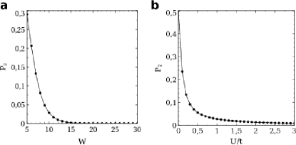
Figure 5: $a)$ representation of $P_{2}$, the weight of the double occupancy states on the ground state wave function, for graphene ribbons as a function of $W$ (for t = 2.7 eV and $U=t$). $b)$ $P_{2}$ as a function of $U/t$, for the ribbon with $W=10$.

Appendix C Electronic dipolar interaction

Here we consider the effect of the dipole-dipole coupling between the magnetization cloud of state $\psi_{A}$ with state $\psi_{B}$. This leads to an additional term in the spin Hamiltonian:

$${\cal H}_{\rm dip}=\sum_{a,b}D_{ab}S_{a}(1)S_{b}(2)$$ (24)

where $a=x,y,z$ and

$$D_{ab}=(g\mu_{B})^{2}\frac{\mu_{0}}{4\pi}\Lambda_{ab}$$ (25)

where

$$\Lambda_{ab}=\sum_{i,i^{\prime}}|\psi_{L}(i)|^{2}|\psi_{R}(i^{\prime})|^{2}\frac{\delta_{a,b}-3n_{a}(ii^{\prime})n_{b}(ii^{\prime})}{r_{ii^{\prime}}^{3}}$$ (26)

where $n_{a}(ii^{\prime})$ is the $a$ component of the unit vector $\vec{n}(ii^{\prime})=\frac{1}{|\vec{r}_{i}-\vec{r}_{i^{\prime}}|}\left(|\vec{r}_{i}-\vec{r}_{i^{\prime}}|\right)$. Of course, the carbon positions lie in the plane $z=0$ so that the $n_{z}$ components are zero. Thus, we have:

$$\Lambda_{zz}=\sum_{i,i^{\prime}}\frac{|\psi_{L}(i)|^{2}|\psi_{R}(i^{\prime})|^{2}}{r_{ii^{\prime}}^{3}}$$ (27)

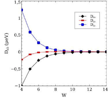
Figure 6: Dipolar interaction, as defined in equation (25), for rectangular graphene nanoribbons, as a function of ribbon size $W$.

Our numerical calculations confirm that only the diagonal terms of the tensor are finite, as expected from symmetry. We show them in figure 6 for rectangular graphene nanoribbons. The elongated shape of ribbons, accounts for the difference between $D_{xx}$ and f $D_{yy}$. The resulting dipolar Hamiltonian can be written as:

$${\cal H}_{\rm dip}=-D_{xx}S_{x}(1)S_{x}(2)+D_{zz}S_{z}(1)S_{z}(2)$$ (28)

Importantly, this Hamiltonian does not couple states with different total $S_{z}$. Therefore, the dipolar interaction does not couple the two states in the two level system formed by the $S=0$ ground state with the $S_{z}=-1$ state (equation (14)). The only effect of the dipolar interaction is to introduce a small anisotropy splitting in the triplet manifold.

Appendix D Hyperfine interaction

The hyperfine interaction is the sum of two dominant contributionsSlichter (2013), Fermi contact interaction and dipolar coupling. The first is given by the overlap of the electronic quantum state with the nuclear species in question. The Fermi-contact contribution to the hyperfine interaction of the edge electron, $A$ or $B$, on a given hydrogen atom, denoted with the label $N$, is computed by calculating the weight of the wave function on the $s$ orbital of that atom and multiplying the weight to the hyperfine interaction of atomic hydrogen, 1024 $MHz$. In order to estimate the contact interaction we adopt a tight-binding model that permits to compute how the $\pi$ orbitals of graphene hybridize with the $s$ orbital of hydrogen. This can be done using the TB model with 4 orbitals per carbon atomFratini et al. (2013); García-Martínez et al. (2015), and one orbital per hydrogen atom. Within this model, the mid-gap states are, in principle, a linear combination of $p_{z}$, $p_{x}$, $p_{y}$ and $s$ orbitals of the carbon atoms and the $s$ orbital of the edge hydrogen atoms. However, for flat structures with mirror symmetry, the $p_{z}$ orbitals are odd under reflection, and are thereby perfectly decoupled from all the other states of the basis set, that are even. As a result, within this model we find that the Fermi contact contribution to the hyperfine interaction vanishes for the mid-gap states, as well as all the low energy states, as long as the edge hydrogen atoms remain in the same plane than the nanographene, which is their equilibrium position.

We thus are left with hyperfine dipolar coupling, whose magnitude we estimate here. Since we are interested in the decoherence induced by the nuclear spins on the electronic states, we treat the nuclear spins as classical magnetic moments $\vec{m}_{N}$, whose orientation is completely random. At any given time they create a magnetic field at a carbon site $\vec{r}_{i}$

$$\vec{B}_{i}[\vec{m}_{N}]=\frac{\mu_{0}}{4\pi}\sum_{N}\frac{\vec{m}_{N}-3\vec{n}_{Ni}\left(\vec{n}_{Ni}\cdot\vec{m}_{N}\right)}{|\vec{r}_{N}-\vec{r}_{i}|^{3}}$$ (29)

where the index $N$ runs over the edge hydrogen atoms and $\vec{n}_{Ni}$ is the unit vector along the direction that joins the nuclear spin $N$ and the carbon site $i$. We now write down the electronic magnetization density as:

$$\vec{m}_{e}(i)=\frac{1}{2}\vec{\tau}_{\sigma,\sigma^{\prime}}\left(|\psi_{A}(i)|^{2}a^{\dagger}_{\sigma}a_{\sigma^{\prime}}+|\psi_{B}(i)|^{2}b^{\dagger}_{\sigma}b_{\sigma^{\prime}}\right)$$ (30)

where $\vec{\tau}_{\sigma,\sigma^{\prime}}$ are the spin $1/2$ Pauli matrices with eigenvalues $\pm 1$. The dipolar hyperfine interaction reads:

$${\cal V}_{N}=-\sum_{i}\vec{m}_{e}(i)\cdot\vec{B}_{i}[\vec{m}_{N}]$$ (31)

It is now convenient to define the average nuclear magnetic field by the electronic states:

$$\vec{\cal B}_{A,B}=\sum_{i}|\psi_{A,B}(i)|^{2}\vec{B}_{i}[\vec{m}_{N}]$$ (32)

This permits to write the interaction of the electronic spins in states $A$ and $B$ with the nuclear spins as:

$${\cal V}_{N}=\sum_{\sigma,\sigma^{\prime}}g\mu_{B}\left(\vec{\cal B}_{A}\cdot\vec{S}^{A}_{\sigma,\sigma^{\prime}}+\vec{\cal B}_{B}\cdot\vec{S}^{B}_{\sigma,\sigma^{\prime}}\right)$$ (33)

where

$$\vec{S}^{A}_{\sigma,\sigma^{\prime}}=\frac{1}{2}\vec{\tau}_{\sigma,\sigma^{\prime}}a^{\dagger}_{\sigma}a_{\sigma^{\prime}},\;\;\;\vec{S}^{B}_{\sigma,\sigma^{\prime}}=\frac{1}{2}\vec{\tau}_{\sigma,\sigma^{\prime}}b^{\dagger}_{\sigma}b_{\sigma^{\prime}}$$ (34)

In the strong coupling limit $\tilde{U}>>\tilde{t}$ this results in the addition of the stochastic magnetic field to the Zeeman contribution in equation (6).

The nuclear field component along the $z$ direction modifies the energy of the $S_{z}=1$ state of the TLS, and leaves the energy of the $S=0$ unchanged. Therefore, it induces a shift of the the TLS splitting, defined by equation (14), by an amount

$$\delta\omega_{0}=\frac{g\mu_{B}}{\hbar}\left({\cal B}_{z,A}+{\cal B}_{z,B}\right)$$ (35)

which is a functional of the nuclear magnetic moments. For nanoribbons and heterojunctions, the mirror symmetry of the structures gives ${\cal B}_{z,A}={\cal B}_{z,B}\equiv{\cal B}_{z,B}$.

We take the orientation of the nuclear moments as random variables with an uniform distribution, given that even at mK temperatures, nuclear Zeeman splitting is much smaller than $k_{B}T$:

$$\langle\vec{m}_{N}\rangle=0\,\,\;,\langle m_{N}^{a}m_{N^{\prime}}^{a^{\prime}}\rangle=\delta_{a,a^{\prime}}\delta_{N,N^{\prime}}\frac{m_{0}^{2}}{3}$$ (36)

where $m_{0}$ is the proton magnetic moment.

As a result, its straightforward to see that the average over nuclear moment realizations vanishes, $\langle\vec{\cal B}_{A.B}\rangle=0$. The standard deviation of the components, defined as:

$${\cal B}_{a,A}^{2}=\frac{\mu_{0}^{2}}{(4\pi)^{2}}\frac{m_{0}^{2}}{3}\sum_{i,i^{\prime},N}\frac{|\psi_{A}(i)|^{2}|\psi_{A}(i^{\prime})|^{2}}{r_{iN}^{3}r_{i^{\prime}N}^{3}}\eta_{a}(N,i,i^{\prime})$$ (37)

where

$$\eta_{a}(N,i,i^{\prime})\equiv 1+9n_{Ni}^{a}n_{Ni^{\prime}}^{a}\vec{n}_{Ni}\cdot\vec{n}_{Ni^{\prime}}-3((n_{Ni}^{a})^{2}+(n_{Ni^{\prime}}^{a})^{2})$$ (38)

In the case of the $a=z$ component we have $n^{z}=0$ for all $N$ and $i$. We can obtain a quick estimate for the edge states in the graphene nanoribbons if we approximate the wave function as equally distributed in 5 edge carbon atoms and only consider their coupling to the first neighbor hydrogen. In that case, we have:

$${\cal B}_{z}^{2}\simeq\frac{\mu_{0}^{2}}{(4\pi)^{2}}\frac{m_{0}^{2}}{3}\frac{1}{d_{HC}^{6}}\equiv\frac{1}{3}\left(b_{0}\right)^{2}$$ (39)

where $d_{H,C}\simeq 1.1\AA$ is the carbon-hydrogen bond length and $b_{0}\simeq 1mT$ is the magnitude of the magnetic field created by a proton at a distance $d_{HC}$. From this, we can estimate the associated shift $\hbar\delta\omega_{0}\simeq 120neV$. Our numerical calculation of (37) yields ${\cal B}_{z}=0.2$ mT for a nanoribbon with $W=10$, in line with the estimate of equation (39)

Appendix E Steady State solution of driven two level system

The steady state solution of the Bloch equation for a two level system driven by an a.c. Rabi monochromatic signal with frequency $\omega$ is given byBaumann et al. (2015)

$$P_{0}-P_{1}=\delta P_{\rm eq}\left(1-\frac{\Omega^{2}T_{1}T_{2}}{1+(\omega-\omega_{0})^{2}T_{2}^{2}+\Omega T_{1}T_{2}}\right)$$ (40)

where $P_{0}$ and $P_{1}$ are the non-equilibrium occupation of the ground and excited states in equation (14) and $\delta P_{\rm eq}\equiv\tanh\left(\frac{\hbar\omega_{0}}{2k_{B}T}\right)$ is the equilibrium population imbalance. Thus, a relevant figure to assess the merit of the electrical control of the spin on electrically driven graphene nanostructures is $x^{2}=\Omega^{2}T_{1}T_{2}$. In resonance, we have $P_{0}-P_{1}=\delta P_{\rm eq}\frac{1}{1+x^{2}}$. Thus, the maximal departure from equilibrium is obtained for very large $x$.

References

- Nielsen and Chuang (2002) M. A. Nielsen and I. Chuang, “Quantum computation and quantum information,” (2002).
- Ardavan and Briggs (2011) A. Ardavan and G. Briggs, Philosophical Transactions of the Royal Society of London A: Mathematical, Physical and Engineering Sciences 369, 3229 (2011).
- Kane (1998) B. E. Kane, Nature 393, 133 (1998).
- Loss and DiVincenzo (1998) D. Loss and D. P. DiVincenzo, Phys. Rev. A 57, 120 (1998).
- Burkard et al. (1999) G. Burkard, D. Loss, and D. P. DiVincenzo, Phys. Rev. B 59, 2070 (1999).
- Gershenfeld and Chuang (1997) N. A. Gershenfeld and I. L. Chuang, science 275, 350 (1997).
- Muhonen et al. (2014) J. T. Muhonen, J. P. Dehollain, A. Laucht, F. E. Hudson, R. Kalra, T. Sekiguchi, K. M. Itoh, D. N. Jamieson, J. C. McCallum, A. S. Dzurak, et al., Nature nanotechnology 9, 986 (2014).
- Elzerman et al. (2004) J. Elzerman, R. Hanson, L. W. Van Beveren, B. Witkamp, L. Vandersypen, and L. P. Kouwenhoven, nature 430, 431 (2004).
- Koppens et al. (2005) F. Koppens, J. Folk, J. Elzerman, R. Hanson, L. W. Van Beveren, I. Vink, H.-P. Tranitz, W. Wegscheider, L. P. Kouwenhoven, and L. Vandersypen, Science 309, 1346 (2005).
- Khaetskii et al. (2002) A. V. Khaetskii, D. Loss, and L. Glazman, Physical review letters 88, 186802 (2002).
- Trauzettel et al. (2007) B. Trauzettel, D. V. Bulaev, D. Loss, and G. Burkard, Nature Physics 3, 192 (2007).
- Laird et al. (2013) E. A. Laird, F. Pei, and L. Kouwenhoven, Nature nanotechnology 8, 565 (2013).
- Steger et al. (2012) M. Steger, K. Saeedi, M. Thewalt, J. Morton, H. Riemann, N. Abrosimov, P. Becker, and H.-J. Pohl, Science 336, 1280 (2012).
- Petta et al. (2005) J. Petta, A. C. Johnson, J. Taylor, E. Laird, A. Yacoby, M. D. Lukin, C. Marcus, M. Hanson, and A. Gossard, Science 309, 2180 (2005).
- Wang et al. (2016) S. Wang, L. Talirz, C. A. Pignedoli, X. Feng, K. Müllen, R. Fasel, and P. Ruffieux, Nature communications 7 (2016).
- Wang et al. (2017) S. Wang, N. Kharche, E. Costa Girão, X. Feng, K. Müllen, V. Meunier, R. Fasel, and P. Ruffieux, Nano Letters (2017).
- Dzyaloshinsky (1958) I. Dzyaloshinsky, Journal of Physics and Chemistry of Solids 4, 241 (1958).
- Moriya (1960) T. Moriya, Physical Review 120, 91 (1960).
- Mani et al. (2012) R. G. Mani, J. Hankinson, C. Berger, and W. A. De Heer, Nature communications 3, 996 (2012).
- Lyon et al. (2017) T. J. Lyon, J. Sichau, A. Dorn, A. Centeno, A. Pesquera, A. Zurutuza, and R. H. Blick, Physical Review Letters 119, 066802 (2017).
- Nakada et al. (1996) K. Nakada, M. Fujita, G. Dresselhaus, and M. S. Dresselhaus, Physical Review B 54, 17954 (1996).
- Fujita et al. (1996) M. Fujita, K. Wakabayashi, K. Nakada, and K. Kusakabe, Journal of the Physical Society of Japan 65, 1920 (1996).
- Wehling et al. (2007) T. Wehling, A. Balatsky, M. Katsnelson, A. Lichtenstein, K. Scharnberg, and R. Wiesendanger, Physical Review B 75, 125425 (2007).
- Yazyev and Helm (2007a) O. V. Yazyev and L. Helm, Phys. Rev. B 75, 125408 (2007a).
- Pereira et al. (2008) V. M. Pereira, J. L. Dos Santos, and A. C. Neto, Physical Review B 77, 115109 (2008).
- Palacios et al. (2008a) J. J. Palacios, J. Fernández-Rossier, and L. Brey, Phys. Rev. B 77, 195428 (2008a).
- Ugeda et al. (2010) M. M. Ugeda, I. Brihuega, F. Guinea, and J. M. Gómez-Rodríguez, Physical Review Letters 104, 096804 (2010).
- González-Herrero et al. (2016) H. González-Herrero, J. M. Gómez-Rodríguez, P. Mallet, M. Moaied, J. J. Palacios, C. Salgado, M. M. Ugeda, J.-Y. Veuillen, F. Yndurain, and I. Brihuega, Science 352, 437 (2016).
- Son et al. (2006a) Y.-W. Son, M. L. Cohen, and S. G. Louie, Physical review letters 97, 216803 (2006a).
- Son et al. (2006b) Y.-W. Son, M. L. Cohen, and S. G. Louie, Nature 444, 347 (2006b).
- Kumazaki and S. Hirashima (2007) H. Kumazaki and D. S. Hirashima, Journal of the Physical Society of Japan 76, 064713 (2007).
- Fernández-Rossier and Palacios (2007) J. Fernández-Rossier and J. J. Palacios, Physical Review Letters 99, 177204 (2007).
- Fernández-Rossier (2008) J. Fernández-Rossier, Physical Review B 77, 075430 (2008).
- Yazyev (2010) O. V. Yazyev, Reports on Progress in Physics 73, 056501 (2010).
- Lado and Fernández-Rossier (2014) J. L. Lado and J. Fernández-Rossier, Phys. Rev. Lett. 113, 027203 (2014).
- García-Martínez et al. (2017) N. A. García-Martínez, J. L. Lado, D. Jacob, and J. Fernández-Rossier, Phys. Rev. B 96, 024403 (2017).
- Cao et al. (2017) T. Cao, F. Zhao, and S. G. Louie, Phys. Rev. Lett. 119, 076401 (2017).
- Ruffieux et al. (2016) P. Ruffieux, S. W. Wang, B. Yang, C. Sánchez, J. Liu, T. Dienel, L. Talirz, P. Shinde, C. A. Pignedoli, D. Passerone, T. Dumslaff, X. Feng, K. Muellen, and R. Fasel, Nature 531, 489 (2016).
- Baumann et al. (2015) S. Baumann, W. Paul, T. Choi, C. P. Lutz, A. Ardavan, and A. J. Heinrich, Science 350, 417 (2015).
- Choi et al. (2017) T. Choi, W. Paul, S. Rolf-Pissarczyk, A. J. Macdonald, F. D. Natterer, K. Yang, P. Willke, C. P. Lutz, and A. J. Heinrich, Nature Nanotechnology 12, 420 (2017).
- Natterer et al. (2017) F. D. Natterer, K. Yang, W. Paul, P. Willke, T. Choi, T. Greber, A. J. Heinrich, and C. P. Lutz, Nature 543, 226 (2017).
- Yang et al. (2017) K. Yang, Y. Bae, W. Paul, F. D. Natterer, P. Willke, J. L. Lado, A. Ferrón, T. Choi, J. Fernández-Rossier, A. J. Heinrich, and C. P. Lutz, Phys. Rev. Lett. 119, 227206 (2017).
- Ortiz et al. (2016) R. Ortiz, J. L. Lado, M. Melle-Franco, and J. Fernández-Rossier, Physical Review B 94, 094414 (2016).
- Kane and Mele (2005) C. L. Kane and E. J. Mele, Phys. Rev. Lett. 95, 146802 (2005).
- Min et al. (2006) H. Min, J. Hill, N. A. Sinitsyn, B. Sahu, L. Kleinman, and A. H. MacDonald, Physical Review B 74, 165310 (2006).
- Konschuh et al. (2010) S. Konschuh, M. Gmitra, and J. Fabian, Physical Review B 82, 245412 (2010).
- Soriano and Fernández-Rossier (2012) D. Soriano and J. Fernández-Rossier, Physical Review B 85, 195433 (2012).
- Yazyev and Helm (2007b) O. V. Yazyev and L. Helm, Phys. Rev. B 75, 125408 (2007b).
- Soriano et al. (2010) D. Soriano, F. Muñoz Rojas, J. Fernández-Rossier, and J. J. Palacios, Phys. Rev. B 81, 165409 (2010).
- Anderson (1959) P. W. Anderson, Phys. Rev. 115, 2 (1959).
- Jafari (2008) S. A. Jafari, Iranian Journal of Physics Research 8, 116 (2008).
- Novoselov et al. (2004) K. S. Novoselov, A. K. Geim, S. V. Morozov, D. Jiang, Y. Zhang, S. V. Dubonos, I. V. Grigorieva, and A. A. Firsov, science 306, 666 (2004).
- Goth and Assaad (2014) F. Goth and F. F. Assaad, Physical Review B 90, 195103 (2014).
- Delgado and Fernández-Rossier (2017) F. Delgado and J. Fernández-Rossier, Progress in Surface Science 92, 40 (2017).
- Slichter (2013) C. P. Slichter, Principles of magnetic resonance, Vol. 1 (Springer Science & Business Media, 2013).
- George et al. (2013) R. E. George, J. P. Edwards, and A. Ardavan, Phys. Rev. Lett. 110, 027601 (2013).
- Pioro-Ladriere et al. (2008) M. Pioro-Ladriere, T. Obata, Y. Tokura, Y.-S. Shin, T. Kubo, K. Yoshida, T. Taniyama, and S. Tarucha, Nature Physics 4, 776 (2008).
- Lado et al. (2017) J. L. Lado, A. Ferrón, and J. Fernández-Rossier, Phys. Rev. B 96, 205420 (2017).
- Carbonell-Sanroma et al. (2017) E. Carbonell-Sanroma , P. Brandimarte, R. Balog, M. Corso, S. Kawai, A. Garcia-Lekue, S. Saito, S. Yamaguchi, E. Meyer, D. Sánchez-Portal, and J. I. Pascual, Nano Letters 17, 50 (2017).
- Chong et al. (0) M. C. Chong, N. Afshar-Imani, F. Scheurer, C. Cardoso, A. Ferretti, D. Prezzi, and G. Schull, Nano Letters 0, null (0).
- Palacios et al. (2008b) J. J. Palacios, J. Fernández-Rossier, and L. Brey, Phys. Rev. B 77, 195428 (2008b).
- Fratini et al. (2013) S. Fratini, D. Gosálbez-Martínez, P. M. Cámara, and J. Fernández-Rossier, Physical Review B 88, 115426 (2013).
- García-Martínez et al. (2015) N. García-Martínez, J. L. Lado, and J. Fernández-Rossier, Physical Review B 91, 235451 (2015).