Positive definite (p.d.) functions vs p.d. distributions

Abstract.

We give explicit transforms for Hilbert spaces associated with positive definite functions on $\mathbb{R}$, and positive definite tempered distributions, incl., generalizations to non-abelian locally compact groups. Applications to the theory of extensions of p.d. functions/distributions are included. We obtain explicit representation formulas for positive definite tempered distributions in the sense of L. Schwartz, and we give applications to Dirac combs and to diffraction. As further applications, we give parallels between Bochner’s theorem (for continuous p.d. functions) on the one hand, and the generalization to Bochner/Schwartz representations for positive definite tempered distributions on the other; in the latter case, via tempered positive measures. Via our transforms, we make precise the respective reproducing kernel Hilbert spaces (RKHSs), that of N. Aronszajn and that of L. Schwartz. Further applications are given to stationary-increment Gaussian processes.

Contents

1. 1 Preliminaries
2. 2 The parallels of p.d. functions vs distributions
3. 3 Dirac Combs, and related Examples
   1. 3.1 The case of IFS-Cantor measures
4. 4 Correspondences and Applications
5. 5 Unimodular groups

The study of positive definite (p.d.) functions and p.d. kernels is motivated by diverse themes in analysis and operator theory, in white noise analysis, applications of reproducing kernel (RKHS) theory, extensions by Laurent Schwartz, and in reflection positivity from quantum physics. Below we make more precise some parallels between, on the one hand, the standard case from Case 1, of continuous positive definite functions $f$ on $\mathbb{R}$, the setting of Bochner’s theorem, including generalizations to non-abelian locally compact groups. We shall also discuss the theory of extensions of p.d. functions. In part two of the paper we obtain representation formulas for positive definite tempered distributions in the sense of L. Schwartz [Sch64a, Sch64b]. The parallels between Bochner’s theorem (for continuous p.d. functions), and the generalization to Bochner/Schwartz representations for positive definite tempered distributions will be made clear. In the first case, we have the Bochner representation via finite positive measures $\mu$; and in the second case, instead via tempered positive measures. This parallel also helps make precise the respective reproducing kernel Hilbert spaces (RKHSs). This further leads to a more unified approach to the treatment of the stationary-increment Gaussian processes [AJL11, AJ12, AJ15]. A key argument will rely on the existence of a unitary representation $U$ of $\left(\mathbb{R},+\right)$, acting on the particular RKHS under discussion. In fact, the same idea (with suitable modifications) will also work in the wider context of locally compact groups. In the abelian case, we shall make use of the Stone representation for $U$ in the form of orthogonal projection valued measures; and in more general settings, the Stone-Naimark-Ambrose-Godement (SNAG) representation [Sto32].

1. Preliminaries

In our theorems and proofs, we shall make use the particular reproducing kernel Hilbert spaces (RKHSs) which allow us to give explicit formulas for our solutions. The general framework of RKHSs were pioneered by Aronszajn in the 1950s [Aro50]; and subsequently they have been used in a host of applications; e.g., [SZ07, SZ09].

The RKHS $\mathscr{H}_{f}$

For simplicity we focus on the case $G=\mathbb{R}$.

Definition 1.1.

Let $\Omega$ be an open domain in $\mathbb{R}$. A function $f:\Omega-\Omega\rightarrow\mathbb{C}$ is positive definite if

$$\sum\nolimits_{i}\sum\nolimits_{j}c_{i}\overline{c}_{j}f\left(x_{i}-x_{j}\right)\geq 0$$ (1.1)

for all finite sums with $c_{i}\in\mathbb{C}$, and all $x_{i}\in\Omega$. We assume that all the p.d. functions are continuous and bounded.

Lemma 1.2 (Two equivalent conditions for p.d.).

If $f$ is given continuous on $\mathbb{R}$, we have the following two equivalent conditions for the positive definite property:

1. $\forall n\in\mathbb{N}$, $\forall\left\{x_{i}\right\}_{1}^{n}$, $\forall\left\{c_{i}\right\}_{1}^{n}$, $x\in\mathbb{R}$, $c_{i}\in\mathbb{C}$,

   $$\sum_{i}\sum_{j}c_{i}\overline{c}_{j}f\left(x_{i}-x_{j}\right)\geq 0;$$

2. $\forall\varphi\in C_{c}\left(\mathbb{R}\right)$, we have:

   $$\int_{\mathbb{R}}\int_{\mathbb{R}}\varphi\left(x\right)\overline{\varphi\left(y\right)}f\left(x-y\right)dxdy\geq 0.$$

Proof.

Use Riemann integral approximation, and note that $f\left(\cdot-x\right)\in\mathscr{H}_{f}$ and $\varphi\ast f\in\mathscr{H}_{f}$. (See details below.) ∎

Consider a continuous positive definite function so $f$ is defined on $\Omega-\Omega$. Set

$$f_{y}\left(x\right):=f\left(x-y\right),\;\forall x,y\in\Omega.$$ (1.2)

Let $\mathscr{H}_{f}$ be the reproducing kernel Hilbert space (RKHS), which is the completion of

$$\left\{\sum\nolimits_{\text{finite}}c_{j}f_{x_{j}}\mid x_{j}\in\Omega,\>c_{j}\in\mathbb{C}\right\}$$ (1.3)

with respect to the inner product

$$\left\langle\sum\nolimits_{i}c_{i}f_{x_{i}},\sum\nolimits_{j}d_{j}f_{y_{j}}\right\rangle_{\mathscr{H}_{f}}:=\sum\nolimits_{i}\sum\nolimits_{j}c_{i}\overline{d}_{j}f\left(x_{i}-y_{j}\right);$$ (1.4)

modulo the subspace of functions of $\left\|\cdot\right\|_{\mathscr{H}_{f}}$-norm zero.

Below, we introduce an equivalent characterization of the RKHS $\mathscr{H}_{f}$, which we will be working with in the rest of the paper.

Lemma 1.3.

Fix $\Omega=(0,\alpha)$. Let $\varphi_{n,x}\left(t\right)=n\varphi\left(n\left(t-x\right)\right)$, for all $t\in\Omega$; where $\varphi$ satisfies

1. $\mathrm{supp}\left(\varphi\right)\subset\left(-\alpha,\alpha\right)$;

2. $\varphi\in C_{c}^{\infty}$, $\varphi\geq 0$;

3. $\int\varphi\left(t\right)dt=1$. Note that $\lim_{n\rightarrow\infty}\varphi_{n,x}=\delta_{x}$, the Dirac measure at $x$.

Lemma 1.4.

The RKHS, $\mathscr{H}_{f}$, is the Hilbert completion of the functions

$$f_{\varphi}\left(x\right)=\int_{\Omega}\varphi\left(y\right)f\left(x-y\right)dy,\;\forall\varphi\in C_{c}^{\infty}\left(\Omega\right),x\in\Omega$$ (1.5)

with respect to the inner product

$$\left\langle f_{\varphi},f_{\psi}\right\rangle_{\mathscr{H}_{f}}=\int_{\Omega}\int_{\Omega}\varphi\left(x\right)\overline{\psi\left(y\right)}f\left(x-y\right)dxdy,\;\forall\varphi,\psi\in C_{c}^{\infty}\left(\Omega\right).$$ (1.6)

In particular,

$$\left\|f_{\varphi}\right\|_{\mathscr{H}_{f}}^{2}=\int_{\Omega}\int_{\Omega}\varphi\left(x\right)\overline{\varphi\left(y\right)}f\left(x-y\right)dxdy,\;\forall\varphi\in C_{c}^{\infty}\left(\Omega\right)$$ (1.7)

and

$$\left\langle f_{\varphi},f_{\psi}\right\rangle_{\mathscr{H}_{f}}=\int_{\Omega}f_{\varphi}\left(x\right)\overline{\psi\left(x\right)}dx,\;\forall\phi,\psi\in C_{c}^{\infty}(\Omega).$$ (1.8)

Proof.

Indeed, by Lemma 1.4, we have

$$\left\|f_{\varphi_{n,x}}-f\left(\cdot-x\right)\right\|_{\mathscr{H}_{f}}\rightarrow 0,\;\mbox{as }n\rightarrow\infty.$$ (1.9)

Hence $\left\{f_{\varphi}\right\}_{\varphi\in C_{c}^{\infty}\left(\Omega\right)}$ spans a dense subspace in $\mathscr{H}_{f}$.

For more details, see [Jor86, Jor87].

∎

These two conditions (1.10)($\Leftrightarrow$(1.11)) below will be used to characterize elements in the Hilbert space $\mathscr{H}_{f}$.

Theorem 1.5.

A continuous function $\xi:\Omega\rightarrow\mathbb{C}$ is in $\mathscr{H}_{f}$ if and only if there exists $A_{0}>0$, such that

$$\sum\nolimits_{i}\sum\nolimits_{j}c_{i}\overline{c}_{j}\xi\left(x_{i}\right)\overline{\xi\left(x_{j}\right)}\leq A_{0}\sum\nolimits_{i}\sum\nolimits_{j}c_{i}\overline{c}_{j}f\left(x_{i}-x_{j}\right)$$ (1.10)

for all finite system $\left\{c_{i}\right\}\subset\mathbb{C}$ and $\left\{x_{i}\right\}\subset\Omega$.

Equivalently, for all $\psi\in C_{c}^{\infty}\left(\Omega\right)$,

$$\left|\int_{\Omega}\psi\left(y\right)\overline{\xi\left(y\right)}dy\right|^{2} \leq A_{0}\int_{\Omega}\int_{\Omega}\psi\left(x\right)\overline{\psi\left(y\right)}f\left(x-y\right)dxdy$$ (1.11)

Note that, if $\xi\in\mathscr{H}_{f}$, then the LHS of (1.11) is $|\left\langle f_{\psi},\xi\right\rangle_{\mathscr{H}_{f}}|^{2}$. Indeed,

$$\left|\left\langle\xi,f_{\psi}\right\rangle_{\mathscr{H}_{f}}\right|^{2} = \left|\left\langle\xi,\int_{\Omega}\psi\left(y\right)f_{y}\>dy\right\rangle_{\mathscr{H}_{f}}\right|^{2}$$

$$= \left|\int_{\Omega}\overline{\psi\left(y\right)}\left\langle\xi,f_{y}\right\rangle_{\mathscr{H}_{f}}dy\right|^{2}$$

$$= \left|\int_{\Omega}\overline{\psi\left(y\right)}\xi\left(y\right)dy\right|^{2}.\;(\text{by the reproducing property})$$

2. The parallels of p.d. functions vs distributions

In this section we prove the following theorem:

Theorem 2.1.

1. Let $f$ be a continuous positive definite (p.d.) function on $\mathbb{R}$ (a p.d. tempered distribution [Sch64a, Sch64b]); then there is a unique finite positive Borel measure $\mu$ on $\mathbb{R}$ (resp., a unique tempered measure on $\mathbb{R}$) such that $f=\widehat{\mu}$.

2. Given $f$ as above, let $\mathscr{H}_{f}$ denote the corresponding kernel Hilbert space, i.e., the Hilbert completion of $\left\{\varphi\ast f\right\}_{\varphi\in C_{c}\left(\Omega\right)}$ (resp. $\varphi\in\mathcal{S}$) w.r.t

   $$\left\|\varphi\ast f\right\|_{\mathscr{H}_{f}}^{2}=\int_{\mathbb{R}}\int_{\mathbb{R}}\varphi\left(x\right)\overline{\varphi\left(y\right)}f\left(x-y\right)dxdy$$

   resp., $\left\langle f\left(x-y\right),\varphi\ast\overline{\varphi}\right\rangle$; action in the sense of distributions. Then there is a unique isometric transform

   $$\mathscr{H}_{f}\xrightarrow{\;T_{f}\;}L^{2}\left(\mathbb{R},\mathscr{B},\mu\right),\quad T_{f}\left(\varphi\ast f\right)=\widehat{\varphi},\;\text{i.e.,}$$

   $$\left\|\varphi\ast f\right\|_{\mathscr{H}_{f}}^{2}=\int_{\mathbb{R}}\left|\widehat{\varphi}\right|^{2}d\mu=\left\|T_{f}\varphi\right\|_{L^{2}\left(\mu\right)}^{2}.$$

3. If $\mu$ is tempered, e.g., if $\int_{\mathbb{R}}\frac{d\mu\left(\lambda\right)}{1+\lambda^{2}}<\infty$, then

   $$\left\|\varphi\ast f\right\|_{\mathscr{H}_{f}}^{2}=\int\left(\left|\widehat{\varphi}\right|^{2}+\big{|}\widehat{\left(D_{x}\varphi\right)}\big{|}^{2}\right)\frac{d\mu\left(\lambda\right)}{1+\lambda^{2}};$$

   where $D_{x}\varphi=\frac{d\varphi}{dx}$, and where “$\widehat{\,\cdot\,}$” denotes the standard Fourier transform on $\mathbb{R}$.

Proof.

The proof will be given below. It will be divided up in a sequence of Lemmas, which by their own merit might be of independent interest. ∎

Corollary 2.2.

Let a function $f$ (or a tempered distribution) be given on a finite open interval in $\mathbb{R}$, but assumed positive definite there; then it automatically has a positive definite extension to $\mathbb{R}$ (in the same category), and so the conclusion of Theorem 2.1 still applies to $f$, or referring to the corresponding p.d. extension.

Proof.

The result uses a main theorem in [JPT16], as well as Lemmas 1.3-1.4 above. ∎

Remark 2.3.

In the case of tempered distributions, the inner product in the RKHS $\mathscr{H}_{f}$ is as follows: First, given $f$ and $\varphi\in\mathcal{S}$, $f$ a p.d. tempered distribution; then the convolution $f\ast\varphi$ is a well defined tempered distribution, and so, for $\psi\in\mathcal{S}$, the expression $\left\langle f\ast\varphi,\overline{\psi}\right\rangle$ denotes the distribution $f\ast\varphi$ applied to $\overline{\psi}\in\mathcal{S}$. Hence, the $\mathscr{H}_{f}$-inner product is:

$$\left\langle f\ast\varphi,f\ast\psi\right\rangle_{\mathscr{H}_{f}}:=\left\langle f\ast\varphi,\overline{\psi}\right\rangle,$$

with this interpretation of action of the distribution $f\ast\varphi$ and the test function $\overline{\psi}$. The p.d. property for $f$ amounts to

$$\left\langle f\ast\varphi,\overline{\varphi}\right\rangle\geq 0,\;\forall\varphi\in\mathcal{S}.$$

Remark 2.4.

The conclusions in the statement of Theorem 2.1 hold also when $\mathbb{R}$ is replaced with an arbitrary locally compact Abelian group $G$. The modification are as follows: Now $f$ will instead be a given continuous p.d. function (or a tempered distribution) on $G$. The modified conclusion (b), see Theorem 2.1, is then:

(b’) $\mathscr{H}_{f}\xmapsto{\;T_{f}\;}L^{2}(\widehat{G},\mathscr{B},\mu)$, $T_{f}\left(\varphi\ast f\right)=\widehat{\varphi}$, and

$$\left\|\varphi\ast f\right\|_{\mathscr{H}_{f}}^{2}=\int_{\widehat{G}}\left|\widehat{\varphi}\right|^{2}d\mu;$$

where $\widehat{G}$ denotes the Pontryagin dual group to $G$, i.e., the group of all continuous characters $\chi$ on $G$; for functions $\varphi$ on $G$ , the transform $\widehat{\varphi}$ is then

$$\widehat{\varphi}\left(\chi\right)=\int_{G}\chi\left(g\right)\varphi\left(g\right)dg$$

with $dg$ denoting Haar measure on $G$; and further $\mu$ is a Borel measure on $\widehat{G}$.

Remark 2.5.

The main theme here is the interconnection between (i) the study of extensions of locally defined continuous and positive definite functions $f$ on groups on the one hand, and, on the other, (ii) the question of extensions for an associated system of unbounded Hermitian operators with dense domain in a reproducing kernel Hilbert space (RKHS) $\mathscr{H}_{f}$ associated to $f$.

The analysis is non-trivial even if $G=\mathbb{R}^{n}$, and even if $n=1$. If $G=\mathbb{R}^{n}$, we are concerned in (ii) with the study of systems of $n$ skew-Hermitian operators $\left\{S_{i}\right\}$ on a common dense domain in Hilbert space, and in deciding whether it is possible to find a corresponding system of strongly commuting selfadjoint operators $\left\{T_{i}\right\}$ such that, for each value of $i$, the operator $T_{i}$ extends $S_{i}$.

The version of this for non-commutative Lie groups $G$ will be stated in the language of unitary representations of $G$, and corresponding representations of the Lie algebra $La\left(G\right)$ by skew-Hermitian unbounded operators.

In summary, for (i) we are concerned with partially defined positive definite continuous functions $f$ on a Lie group; i.e., at the outset, such a function $f$ will only be defined on a connected proper subset in $G$. From this partially defined p.d. function $f$ we then build a reproducing kernel Hilbert space $\mathscr{H}_{f}$, and the operator extension problem (ii) is concerned with operators acting on $\mathscr{H}_{f}$, as well as with unitary representations of $G$ acting on $\mathscr{H}_{f}$. If the Lie group $G$ is not simply connected, this adds a complication, and we are then making use of the associated simply connected covering group.

Because of the role of positive definite functions in harmonic analysis, in statistics, and in physics, the connections in both directions is of interest, i.e., from (i) to (ii), and vice versa. This means that the notion of “extension” for question (ii) must be inclusive enough in order to encompass all the extensions encountered in (i). For this reason enlargement of the initial Hilbert space $\mathscr{H}_{f}$ are needed. In other words, it is necessary to consider also operator extensions which are realized in a dilation-Hilbert space; a new Hilbert space containing $\mathscr{H}_{f}$ isometrically, and with the isometry intertwining the respective operators.

For more details, we refer the reader to [JPT16] and the papers cited there.

Key steps in the present application is the identification of a unitary representation $\left\{U_{t}\right\}_{t\in\mathbb{R}}$ acting in the RKHS $\mathscr{H}_{f}$; it applies both when $f$ is continuous and p.d. (Bochner), and when $f$ is a p.d. tempered distribution (Schwartz [Sch64a, Sch64b])

$$U_{t}\left(\varphi\ast f\right):=\varphi\left(\cdot-t\right)\ast f=\varphi\ast f\left(\cdot+t\right).$$

One concludes that

1. $U_{t_{1}}U_{t_{2}}=U_{t_{1}+t_{2}}$, $\forall t_{i}\in\mathbb{R}$; and

2. $U_{t}$ is strongly continuous, i.e., $\lim_{t\rightarrow 0}\left\|U_{t}w-w\right\|_{\mathscr{H}_{f}}=0$ holds for $\forall w\in\mathscr{H}_{f}$.

Now assume that $f$ is p.d., and let $\left\{U_{t}\right\}_{t\in\mathbb{R}}$ be the unitary group acting in the corresponding RKHS. By Stone’s theorem [Sto32], there exists a projection valued measure $E$ on $\left(\mathbb{R},\mathscr{B}\right)$, $\mathscr{B}=$ Borel sigma-algebra in $\mathbb{R}$. That is, $E:\mathscr{B}\rightarrow\text{proj}(\mathscr{H}_{f})$ satisfying

$$E\left(B\right)^{*} =E\left(B\right)=E\left(B\right)^{2}, \forall B\in\mathscr{B}$$ (2.1)

$$E\left(B\cap C\right) =E\left(B\right)=E\left(C\right), \forall B,C\in\mathscr{B}$$ (2.2)

such that

$$U_{t}=\int_{\mathbb{R}}e^{i\lambda t}E\left(d\lambda\right),\;t\in\mathbb{R}.$$ (2.3)

(See, e.g., [Sto32].)

Lemma 2.6.

Let $f$, $\mathscr{H}_{f}$, $\left\{U_{t}\right\}_{t\in\mathbb{R}}$ be as above. Let $w_{0}=f\left(\cdot-0\right)\in\mathscr{H}_{f}$, and set

$$\mu:=\left\|E\left(d\lambda\right)w_{0}\right\|_{\mathscr{H}_{f}}^{2}$$ (2.4)

then

$$\left\|\varphi\ast f\right\|_{\mathscr{H}_{f}}^{2}=\int_{\mathbb{R}}\left|\widehat{\varphi}\left(\lambda\right)\right|^{2}d\mu\left(\lambda\right).$$ (2.5)

Proof.

(2.4)$\Rightarrow$(2.5) For $\varphi\in C_{c}\left(\mathbb{R}\right)$, we have

$$\varphi\ast f:=\int_{\mathbb{R}}\varphi\left(t\right)f\left(\cdot-t\right)dt=\int\varphi\left(t\right)U_{t}w_{0}\,dt\;\left(\text{by $\left(\ref{eq:a1}\right)$, $\left(\ref{eq:a4}\right)$}\right)$$

i.e., convolution, and

$$\varphi\ast f = \int_{\mathbb{R}}\varphi\left(t\right)U_{t}w_{0}dt$$

$$\underset{\text{by $\left(\ref{eq:a3}\right)$}}{=} \int_{\mathbb{R}}\varphi\left(t\right)\int e^{it\lambda}\underset{\text{PVM}}{\underbrace{E\left(d\lambda\right)}}w_{0}dt$$

$$\underset{\left(\text{Fubini}\right)}{=} \int_{\mathbb{R}}\left(\int_{\mathbb{R}}\varphi\left(t\right)e^{it\lambda}dt\right)E\left(d\lambda\right)w_{0}$$

$$\int_{\mathbb{R}}\widehat{\varphi}\left(\lambda\right)E\left(d\lambda\right)w_{0}.$$

It follows that

$$\left\|\varphi\ast f\right\|_{\mathscr{H}_{f}}^{2} \underset{\text{by $\left(\ref{eq:a2}\right)$}}{=} \int_{\mathbb{R}}\left|\widehat{\varphi}\left(\lambda\right)\right|^{2}\left\|E\left(d\lambda\right)w_{0}\right\|_{\mathscr{H}_{f}}^{2}$$

$$\underset{\text{by $\left(\ref{eq:a4}\right)$}}{=} \int_{\mathbb{R}}\left|\widehat{\varphi}\left(\lambda\right)\right|^{2}d\mu\left(\lambda\right),$$

i.e., use $\left\langle E\left(d\lambda_{1}\right)w_{0},E\left(d\lambda_{2}\right)w_{0}\right\rangle_{\mathscr{H}_{f}}=\left\langle w_{0},E\left(d\lambda_{1}d\lambda_{2}\right)w_{0}\right\rangle_{\mathscr{H}_{f}}=\left\|E\left(d\lambda\right)w_{0}\right\|_{\mathscr{H}_{f}}^{2}$. ∎

Conclusion. The RKHS $\mathscr{H}_{f}$ is the completion of $\varphi\ast f$, $\varphi\in C_{c}\left(\mathbb{R}\right)$, with respect to the norm $\int\left|\widehat{\varphi}\left(\lambda\right)\right|^{2}d\mu\left(\lambda\right)$, via the mapping $\varphi\ast f\longmapsto\widehat{\varphi}\in L^{2}\left(\mathbb{R},\mu\right)$.

Remark 2.7.

Note that the proof is mutatis mutandis to the case of positive definite tempered distributions in the sense of L. Schwartz [Sch64a, Sch64b].

We also get an extension of $\varphi\ast f$ to $\varphi\ast h$, $\forall h\in\mathscr{H}_{f}\left(=\text{RKHS}\right)$ as follows.

First define $\left\{U_{t}\right\}_{t\in\mathbb{R}}$ as a unitary representation of $\left(\mathbb{R},+\right)$ on $\mathscr{H}_{f}$; and then, for $h\in\mathscr{H}_{f}$, set ($\varphi\in C_{c}\left(\mathbb{R}\right)$, or $\varphi\in\mathcal{S}$)

$$\varphi\ast h=\int_{\mathbb{R}}\varphi\left(t\right)U_{t}h\>dt.$$

Then we have:

$$\left\|\varphi\ast h\right\|_{\mathscr{H}_{f}}\leq\left(\int_{\mathbb{R}}\left|\varphi\left(t\right)\right|dt\right)\left\|h\right\|_{\mathscr{H}_{f}}=\left\|\varphi\right\|_{L^{1}}\left\|h\right\|,\;\forall\varphi\in\mathcal{S},\>\forall h\in\mathscr{H}_{f}.$$

Corollary 2.8.

For every tempered positive definite measure $\mu$ (see Theorem 2.1) there is a unique Gaussian process $X=X^{\left(\mu\right)}$ indexed by $x\in\mathbb{R}$, with mean zero, and variance

$$r^{\left(\mu\right)}\left(x\right)=\mathbb{E}\left(\big{|}X_{x}^{\left(\mu\right)}\big{|}^{2}\right)=\int_{\mathbb{R}}\left|1-e^{i\lambda x}\right|^{2}\frac{d\mu\left(\lambda\right)}{\lambda^{2}},$$

and in addition,

$$\mathbb{E}\left(X_{x}^{\left(\mu\right)}\overline{X_{y}^{\left(\mu\right)}}\right)=\frac{r^{\left(\mu\right)}\left(\left|x\right|\right)+r^{\left(\mu\right)}\left(\left|y\right|\right)-r^{\left(\mu\right)}\left(\left|x-y\right|\right)}{2},$$

and

$$\mathbb{E}\left(\big{|}X_{x}^{\left(\mu\right)}-X_{y}^{\left(\mu\right)}\big{|}^{2}\right)=r^{\left(\mu\right)}\left(\left|x-y\right|\right).$$

Proof.

This family of stationary increment Gaussian processes were studied in [AJL11], and so we omit details here. The idea is to apply the transform $T_{\mu}$ from Theorem 2.1 (b) to the associated Gaussian process.

Setting $\varphi_{x}=\varphi=\begin{cases}\chi_{\left[0,x\right]}\left(\cdot\right)&\text{if }x\geq 0\\ -\chi_{\left[0,x\right]}\left(\cdot\right)&\text{if }x<0\end{cases}$ , we get

$$r^{\left(\mu\right)}\left(x\right) =\int_{\mathbb{R}}\left|\widehat{\varphi}\left(\lambda\right)\right|^{2}d\mu\left(\lambda\right)\quad(\text{see Thm. \ref{thm:p1} (b)})$$

$$=\int_{\mathbb{R}}\left|1-e^{i\lambda x}\right|^{2}\frac{d\mu\left(\lambda\right)}{\lambda^{2}},\;x\in\mathbb{R},$$

as claimed. ∎

3. Dirac Combs, and related Examples

In Theorem 2.1, we made a distinction between the two cases: that of (i) continuous p.d. functions, and (ii) the case of positive definite tempered distributions. The two cases are connected with the studies of Aronszajn [Aro50], in case (i); and of Schwartz [Sch64b], in case (ii). In the present section, we illustrate this distinction in detail.

To review the conclusions in Theorem 2.1, in case (i), the Hilbert completion $\mathscr{H}_{f}$ of $\left\{\varphi\ast f\mathrel{;}\varphi\in C_{c}\left(\mathbb{R}\right)\right\}$ in the pre-Hilbert inner product

$$\int_{\mathbb{R}}\int_{\mathbb{R}}\varphi\left(x\right)\overline{\varphi\left(y\right)}f\left(x-y\right)dxdy$$ (3.1)

is a reproducing kernel Hilbert space (RKHS) in the sense of Aronszajn. The reason is that, for all $x\in\mathbb{R}$, the function $f\left(\cdot-x\right)$ is in $\mathscr{H}_{f}$, and

$$\left\langle f\left(\cdot-x\right),h\right\rangle_{\mathscr{H}_{f}}=h\left(x\right),\;\forall x\in\mathbb{R},\>\forall h\in\mathscr{H}_{f};$$ (3.2)

i.e., $\mathscr{H}_{f}$ satisfies the Aronszajn reproducing property. This is not so in case (ii), but nonetheless, we shall get a reproducing property in the measure theoretic setting from the paper [Sch64b] of L. Schwartz.

The above conclusions are made precise in the following:

Proposition 3.1 (The Dirac comb [BJV16, GP16, KL13]).

Set

$$\mu:=\sum_{n\in\mathbb{Z}}\delta_{n}$$ (3.3)

where $\delta_{n}$ in (3.3) denotes the Dirac distribution. Then $f=\widehat{\mu}$ is the tempered Schwartz distribution, written formally as

$$f\left(x\right)=\sum_{n\in\mathbb{Z}}e^{inx},\;x\in\mathbb{R}.$$ (3.4)

In this case the Hilbert completion $\mathscr{H}_{f}$ from Theorem 2.1 is the Hilbert space of all $2\pi$-periodic functions $h$ on $\mathbb{R}$ subject to the condition

$$\left\|h\right\|_{\mathscr{H}_{f}}^{2}:=\frac{1}{2\pi}\int_{-\pi}^{\pi}\left|h\left(x\right)\right|^{2}dx<\infty.$$ (3.5)

Proof.

A positive measure $\mu$ on $\mathbb{R}$ is said to be tempered iff $\exists M\in\mathbb{N}$ such that

$$\int_{\mathbb{R}}\frac{d\mu\left(\lambda\right)}{1+\lambda^{2M}}<\infty.$$ (3.6)

The measure $\mu$ in (3.3) is clearly tempered, and in particular it is $\sigma$-finite. Specifically if $B\in\mathscr{B}_{\mathbb{R}}$ (the Borel $\sigma$-algebra), then

$$\mu\left(B\right)=\#\left(B\cap\mathbb{Z}\right).$$ (3.7)

For $M$ in (3.6) we may take $M=1$.

We now turn to the Hilbert completion $\mathscr{H}_{f}$ where $f$ is as in (3.4). For all test-function $\varphi\in\mathcal{S}$, we have:

$$\left(\varphi\ast f\right)\left(x\right)=\sum_{n\in\mathbb{Z}}\widehat{\varphi}\left(n\right)e^{-inx}$$ (3.8)

where the interpretation of (3.8) is in the sense of tempered Schwartz distributions. Moreover,

$$\int_{\mathbb{R}}\int_{\mathbb{R}}\varphi\left(x\right)\overline{\varphi\left(y\right)}f\left(x-y\right)dxdy=\sum_{n\in\mathbb{Z}}\left|\widehat{\varphi}\left(n\right)\right|^{2}.$$ (3.9)

Now, combining (3.8) and (3.9), we get that $\mathscr{H}_{f}$ is the Hilbert space described before (3.5). To see this, we apply the Plancherel-Fourier theorem, i.e., for $\forall\left(c_{n}\right)\in l^{2}$, the function $h\left(x\right)=\sum_{n\in\mathbb{Z}}c_{n}e^{inx}$ is well defined, and

$$\frac{1}{2\pi}\int_{-\pi}^{\pi}\left|h\left(x\right)\right|^{2}dx=\sum_{n\in\mathbb{Z}}\left|c_{n}\right|^{2}.$$ (3.10)

Comparing now with (3.8), the desired conclusion follows. ∎

Remark 3.2.

By the Poisson summation formula, (3.4) can also be written as

$$f\left(x\right)=\sum_{n\in\mathbb{Z}}e^{inx}=2\pi\sum_{n\in\mathbb{Z}}\delta\left(x-2\pi n\right).$$

3.1. The case of IFS-Cantor measures

Let $\nu=\nu_{4}$ be the scale 4-Cantor fractal measure (see [JP93, JP98]) specified by the IFS-identity:

$$\frac{1}{2}\int\left(h\left(\frac{x}{4}\right)+h\left(\frac{x+2}{4}\right)\right)d\nu_{4}\left(x\right)=\int h\left(x\right)d\nu_{4}\left(x\right)$$ (3.11)

for all $h$. Introduce the transform

$$\widehat{\nu}\left(\xi\right):=\int_{\mathbb{R}}e^{i\xi x}d\nu\left(x\right),$$ (3.12)

and (3.11) is equivalent to

$$\widehat{\nu}_{4}\left(\xi\right)=\frac{1+e^{i\xi/2}}{2}\widehat{\nu}_{4}\left(\xi/4\right),\;\forall\xi\in\mathbb{R}.$$ (3.13)

Note that, as a consequence, the support of this cantor measure $\nu_{4}$ is then precisely the scale-4 Cantor set from Fig 3.1 above. It was shown by Jorgensen-Pedersen [JP98] that $L^{2}\left(\nu_{4}\right)$ has an orthonormal basis (ONB) of functions $e_{\lambda}\left(x\right):=e^{i\lambda x}$. One may take for example

$$\Lambda_{4} :=\left\{0,1,4,5,16,17,20,21,64,65,\cdots\right\}$$

$$=\left\{\sum\nolimits_{0}^{\text{finite}}b_{j}4^{j}\mathrel{;}b_{j}\in\left\{0,1\right\}\right\}.$$ (3.14)

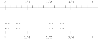
Figure 3.1. The $\frac{1}{4}$-Cantor set.

While $\left\{e_{\lambda}\mathrel{;}\lambda\in\Lambda_{4}\right\}$ forms an ONB in $L^{2}\left(\nu_{4}\right)$, we say that $\left(\nu_{4},\Lambda_{4}\right)$ is a spectral pair, it should be stressed that many Cantor measures $\nu$ do not allow ONBs of the form $\left\{e_{\lambda}\mathrel{;}\lambda\in\Lambda\right\}$ for any subsets $\Lambda$ of $\mathbb{R}$; for example $\nu_{3}$ is the opposite extreme: Jorgensen & Pedersen proved that $L^{2}\left(\nu_{3}\right)$ does not admit more than two orthogonal functions of the form $e_{\lambda}\left(x\right)=e^{i\lambda x}$, $\lambda\in\mathbb{R}$. By $\nu_{3}$, we mean the unique Borel probability measure satisfying

$$\frac{1}{2}\int\left(h\left(\frac{x}{3}\right)+h\left(\frac{x+2}{3}\right)\right)d\nu_{3}\left(x\right)=\int h\left(x\right)d\nu_{3}\left(x\right),$$ (3.15)

for all $h$, compare (3.11) with above.

Using now the same ideas from the present paper, we get the following:

Proposition 3.3.

Let $\left(\nu_{4},\Lambda_{4}\right)$ be as above; see (3.11)-(3.14), and set

$$\mu_{4}:=\sum_{\lambda\in\Lambda_{4}}\delta_{\lambda},$$

and

$$f_{4}\left(x\right):=\sum_{\lambda\in\Lambda_{4}}e^{i\lambda x},\;x\in\mathbb{R},$$

realized as a tempered p.d. distribution. Let $\mathscr{H}_{f_{4}}$ be the associated Hilbert space from Theorem 2.1. Then there is a natural isometric isomorphism between the two Hilbert spaces $\mathscr{H}_{f_{4}}$ and $L^{2}\left(\nu_{4}\right)$.

Proof.

The details are the same as those of the proof of Proposition 3.1. The key step is use of the fact from [JP98] that $\left\{e_{\lambda}\mathrel{;}\lambda\in\Lambda_{4}\right\}$ is an ONB in the Hilbert space $L^{2}\left(\nu_{4}\right)$ defined from the Cantor measure $\nu_{4}$. ∎

4. Correspondences and Applications

Continuous p.d. functions on $\mathbb{R}$

Lemma.

Let $f$ be a continuous function on $\mathbb{R}$. Then the following are equivalent:

1. $f$ is p.d., i.e., $\forall\varphi\in C_{c}\left(\mathbb{R}\right)$, we have

   $$\int_{\mathbb{R}}\int_{\mathbb{R}}\varphi\left(x\right)\overline{\varphi\left(y\right)}f\left(x-y\right)dxdy\geq 0.$$ (4.1)

2. $\forall\left\{x_{j}\right\}_{j=1}^{n}\subset\mathbb{R}$, $\forall\left\{c_{j}\right\}_{j=1}^{n}\subset\mathbb{C}$, and $\forall n\in\mathbb{N}$, we have

   $$\sum_{j=1}^{n}\sum_{k=1}^{n}c_{j}\overline{c}_{k}f\left(x_{j}-x_{k}\right)\geq 0.$$ (4.2)

p.d. tempered distributions on $\mathbb{R}$

Lemma.

Let $f$ be a tempered distribution on $\mathbb{R}$. Then $f$ is p.d. if and only if

$$\int_{\mathbb{R}}\int_{\mathbb{R}}\varphi\left(x\right)\overline{\varphi\left(y\right)}f\left(x-y\right)dxdy\geq 0$$ (4.3)

hold, for all $\varphi\in\mathcal{S}$, where $\mathcal{S}$ is the Schwartz space.

Equivalently,

$$\left\langle f\left(x-y\right),\varphi\otimes\overline{\varphi}\right\rangle\geq 0,\;\forall\varphi\in\mathcal{S}.$$ (4.4)

Here $\left\langle\cdot,\cdot\right\rangle$ denotes distribution action.

RKHS

Bochner’s theorem.

$\exists!$ positive finite measure $\mu$ on $\mathbb{R}$ such that

$$f\left(x\right)=\int_{\mathbb{R}}e^{ix\lambda}d\mu\left(\lambda\right).$$

Bochner/Schwartz

$\exists$ positive tempered measure $\mu$ on $\mathbb{R}$ such that

$$f=\widehat{\mu}$$

where $\widehat{\mu}$ is in the sense of distribution.

Let $\mathscr{H}_{f}$ be the RKHS of $f$.

• Then

  $$\left\|\varphi\ast f\right\|_{\mathscr{H}_{f}}^{2}=\int_{\mathbb{R}}\left|\widehat{\varphi}\left(\lambda\right)\right|^{2}d\mu\left(\lambda\right)$$ (4.5)

  where $\widehat{\varphi}=$ the Fourier transform.

• $f$ admits the factorization

  $$f\left(x_{1}-x_{2}\right)=\left\langle f\left(\cdot-x_{1}\right),f\left(\cdot-x_{2}\right)\right\rangle_{\mathscr{H}_{f}}$$

  $\forall x_{1},x_{2}\in\mathbb{R}$, with

  $\mathbb{R}\ni x\longrightarrow f\left(\cdot-x\right)\in\mathscr{H}_{f}$.

Let $\mathscr{H}_{f}$ denote the corresponding RKHS.

• For all $\varphi\in\mathcal{S}$, we have

  $$\left\|\varphi\ast f\right\|_{\mathscr{H}_{f}}^{2}=\left\langle f\left(x-y\right),\varphi\otimes\overline{\varphi}\right\rangle,$$ (4.6)

  distribution action.

• $\mathcal{S}\ni\varphi\longmapsto\varphi\ast f\in\mathscr{H}_{f}$, where

  $$\left(\varphi\ast f\right)\left(\cdot\right)=\int\varphi\left(y\right)f\left(\cdot-y\right)dy.$$

Applications

Now applied to Bochner’s theorem.

Set $\mathscr{H}_{f}=$ RKHS of $f$, and $w_{0}=f\left(\cdot-0\right)$. Then

$$U_{t}w_{0}=w_{t}=f\left(\cdot-t\right),\;t\in\mathbb{R}$$

defines a strongly continuous unitary representation of $\mathbb{R}$.

On white noise space:

$$\mathbb{E}\left(e^{i\left\langle\varphi,\cdot\right\rangle}\right)=e^{-\frac{1}{2}\int\left|\widehat{\varphi}\right|^{2}d\mu}$$

where $\mathbb{E}\left(\cdots\right)=$ expectation w.r.t the Gaussian path-space measure.

(The proof for the special case when $f$ is assumed p.d. and continuous carries over with some changes to the case when $f$ is a p.d. tempered distribution.)

Note.

In both cases, we have the following representation for vectors in the RKHS $\mathscr{H}_{f}$:

$$\left\langle\varphi\ast f,\psi\ast f\right\rangle_{\mathscr{H}_{f}}=\left\langle\varphi\ast\overline{\psi},f\right\rangle,\;\forall\varphi,\psi\in\mathcal{S};$$ (4.7)

where $\varphi\ast f:=$ the standard convolution w.r.t. Lebesgue measure.

5. Unimodular groups

Let $G$ be a locally compact group, and assume it is unimodular, i.e., its Haar measure is both left and right invariant. By a theorem of I.E. Segal, there is then a Plancherel theorem for the unitary representations of $G$ (see [Seg50] and [Mac89, Mac76, Mac92]). If $C^{*}\left(G\right)$ denotes the group algebra with convolution product

$$\left(\varphi\ast\psi\right)\left(x\right)=\int_{G}\varphi\left(y\right)\psi\left(y^{-1}x\right)dy,$$ (5.1)

where $\varphi$, $\psi$ are functions on $G$, and $dy$ denotes the Haar measure. The $\ast$-operation in (5.1) is

$$\varphi^{*}\left(x\right)=\overline{\varphi\left(x^{-1}\right)},\;x\in G.$$ (5.2)

Then $C^{*}\left(G\right)$ is the $C^{*}$-completion of this $*$-algebra.

Note that since $G$ is assumed unimodular, we need not include the modular function $\Delta$ in the definition (5.2). By general theory, it is known that the set of equivalence classes of irreducible unitary representations of $G$ is then in bijective correspondence with the set $P\left(G\right)$ of pure states of $C^{*}\left(G\right)$.

Lemma 5.1.

(a) Let $G$ be a unimodular (locally compact) group, and let $f$ be a continuous positive definite function on $G$. Let $\mathscr{H}_{f}$ be the corresponding reproducing kernel Hilbert space (RKHS) If $\pi$ is an irreducible unitary representation of $G$, we denote by $\lambda_{\pi}$ the corresponding state. More precisely,

$$\lambda_{\pi}\left(x\right)=\left\langle v,\pi\left(x\right)v\right\rangle_{\mathscr{H}_{\pi}},\;x\in G$$ (5.3)

defines a pure state, $\lambda_{\pi}\in P\left(G\right)$.

(b) Given $f$ p.d. and continuous as above, there is a unique Borel measure $\mu=\mu_{f}$ concentrated on $P\left(G\right)$ such that

$$\left\|\varphi\ast f\right\|_{\mathscr{H}_{f}}^{2}=\int_{P\left(G\right)}\left|\lambda_{\pi}\left(\varphi\right)\right|^{2}d\mu\left(\lambda_{\pi}\right).$$ (5.4)

Proof.

First a caution, the set $P\left(G\right)$ may not in general be a Borel set, but by a theorem of Phelphs [Phe77], the measure $\mu$ may be chosen on a Borel set $B$ such that

$$\mu\left(B\,\Delta\,P\left(G\right)\right)=0$$ (5.5)

where $\Delta$ denotes “symmetric difference.”

Other than this point, the present proof follows closely that of Section 2 (in the Abelian case).

We introduce $\mathscr{H}_{f}$ as the completion of the functions $\varphi\ast f$ (convolution) for $\varphi\in C_{c}\left(G\right)$:

$$\left\|\varphi\ast f\right\|_{\mathscr{H}_{f}}^{2}=\int_{G}\left(\varphi\ast\varphi^{*}\right)\left(x\right)f\left(x\right)dx,$$

see (5.1)-(5.1); with $dx$ denotes Haar measure. As before, we get a unitary representation $U$ of $G$ acting in $\mathscr{H}_{f}$ via

$$U_{x}\left(\varphi\ast f\right)=\varphi\left(x^{-1}\cdot\right)\ast f,$$

and $\left(\left\{U_{x}\right\}_{x\in G},\mathscr{H}_{f}\right)$ then decomposes as per the Plancherel theorem for $G$. Hence there exists a unique $\mu$ on $P\left(G\right)$ such that

$$U=\int_{P\left(G\right)}\pi\,d\mu\left(\lambda_{\pi}\right),$$

and the result follows. ∎

Acknowledgement.

The co-authors thank the following colleagues for helpful and enlightening discussions: Professors Daniel Alpay, Sergii Bezuglyi, Ilwoo Cho, A. Jaffe, Paul Muhly, K.-H. Neeb, G. Olafsson, Wayne Polyzou, Myung-Sin Song, and members in the Math Physics seminar at The University of Iowa.

References

• [AJ12] Daniel Alpay and Palle E. T. Jorgensen, Stochastic processes induced by singular operators, Numer. Funct. Anal. Optim. 33 (2012), no. 7-9, 708–735. MR 2966130
• [AJ15] Daniel Alpay and Palle Jorgensen, Spectral theory for Gaussian processes: reproducing kernels, boundaries, and $L^{2}$-wavelet generators with fractional scales, Numer. Funct. Anal. Optim. 36 (2015), no. 10, 1239–1285. MR 3402823
• [AJL11] Daniel Alpay, Palle Jorgensen, and David Levanony, A class of Gaussian processes with fractional spectral measures, J. Funct. Anal. 261 (2011), no. 2, 507–541. MR 2793121
• [Aro50] N. Aronszajn, Theory of reproducing kernels, Trans. Amer. Math. Soc. 68 (1950), 337–404. MR 0051437
• [BJV16] Maria Alice Bertolim, Alain Jacquemard, and Gioia Vago, Integration of a Dirac comb and the Bernoulli polynomials, Bull. Sci. Math. 140 (2016), no. 2, 119–139. MR 3456185
• [GP16] Bertrand G. Giraud and Robi Peschanski, From “Dirac combs” to Fourier-positivity, Acta Phys. Polon. B 47 (2016), no. 4, 1075–1100. MR 3494188
• [Jor86] Palle E. T. Jorgensen, Analytic continuation of local representations of Lie groups, Pacific J. Math. 125 (1986), no. 2, 397–408. MR 863534 (88m:22030)
• [Jor87] by same author, Analytic continuation of local representations of symmetric spaces, J. Funct. Anal. 70 (1987), no. 2, 304–322. MR 874059
• [JP93] Palle E. T. Jorgensen and Steen Pedersen, Harmonic analysis of fractal measures induced by representations of a certain $C^{*}$-algebra, Bull. Amer. Math. Soc. (N.S.) 29 (1993), no. 2, 228–234. MR 1215311
• [JP98] by same author, Dense analytic subspaces in fractal $L^{2}$-spaces, J. Anal. Math. 75 (1998), 185–228. MR 1655831
• [JPT16] Palle Jorgensen, Steen Pedersen, and Feng Tian, Extensions of positive definite functions, Lecture Notes in Mathematics, vol. 2160, Springer, [Cham], 2016, Applications and their harmonic analysis. MR 3559001
• [KL13] Johannes Kellendonk and Daniel Lenz, Equicontinuous Delone dynamical systems, Canad. J. Math. 65 (2013), no. 1, 149–170. MR 3004461
• [Mac76] George W. Mackey, The theory of unitary group representations, University of Chicago Press, Chicago, Ill.-London, 1976, Based on notes by James M. G. Fell and David B. Lowdenslager of lectures given at the University of Chicago, Chicago, Ill., 1955, Chicago Lectures in Mathematics. MR 0396826
• [Mac89] by same author, Unitary group representations in physics, probability, and number theory, second ed., Advanced Book Classics, Addison-Wesley Publishing Company, Advanced Book Program, Redwood City, CA, 1989. MR 1043174
• [Mac92] by same author, Harmonic analysis and unitary group representations: the development from 1927 to 1950, L’émergence de l’analyse harmonique abstraite (1930–1950) (Paris, 1991), Cahiers Sém. Hist. Math. Sér. 2, vol. 2, Univ. Paris VI, Paris, 1992, pp. 13–42. MR 1187300
• [Phe77] R. R. Phelps, The Choquet representation in the complex case, Bull. Amer. Math. Soc. 83 (1977), no. 3, 299–312. MR 0435818
• [Sch64a] L. Schwartz, Sous-espaces hilbertiens et noyaux associés; applications aux représentations des groupes de Lie, Deuxième Colloq. l’Anal. Fonct, Centre Belge Recherches Math., Librairie Universitaire, Louvain, 1964, pp. 153–163. MR 0185423
• [Sch64b] Laurent Schwartz, Sous-espaces hilbertiens d’espaces vectoriels topologiques et noyaux associés (noyaux reproduisants), J. Analyse Math. 13 (1964), 115–256. MR 0179587
• [Seg50] I. E. Segal, An extension of Plancherel’s formula to separable unimodular groups, Ann. of Math. (2) 52 (1950), 272–292. MR 0036765
• [Sto32] M. H. Stone, On one-parameter unitary groups in Hilbert space, Ann. of Math. (2) 33 (1932), no. 3, 643–648. MR 1503079
• [SZ07] Steve Smale and Ding-Xuan Zhou, Learning theory estimates via integral operators and their approximations, Constr. Approx. 26 (2007), no. 2, 153–172. MR 2327597
• [SZ09] by same author, Geometry on probability spaces, Constr. Approx. 30 (2009), no. 3, 311–323. MR 2558684