Bose–Einstein correlations in $\Pp\Pp$, $\Pp$Pb, and PbPb collisions at $\sqrt{\smash[b]{s_{{}_{\text{NN}}}}}=$ 0.9–7

Abstract

Quantum statistical (Bose–Einstein) two-particle correlations are measured in pp collisions at $\sqrt{s}=0.9$, 2.76, and 7, as well as in $\Pp$Pb and peripheral PbPb collisions at nucleon-nucleon center-of-mass energies of 5.02 and 2.76, respectively, using the CMS detector at the LHC. Separate analyses are performed for same-sign unidentified charged particles as well as for same-sign pions and kaons identified via their energy loss in the silicon tracker. The characteristics of the one-, two-, and three-dimensional correlation functions are studied as functions of the pair average transverse momentum ($\kt$) and the charged-particle multiplicity in the event. For all systems, the extracted correlation radii steadily increase with the event multiplicity, and decrease with increasing $\kt$. The radii are in the range 1–5fm, the largest values corresponding to very high multiplicity $\Pp$Pb interactions and to peripheral PbPb collisions with multiplicities similar to those seen in $\Pp$Pb data. It is also observed that the dependencies of the radii on multiplicity and $\kt$ largely factorize. At the same multiplicity, the radii are relatively independent of the colliding system and center-of-mass energy.

0.1 Introduction

Studies of quantum-statistical correlations of pairs of identical particles produced in high-energy collisions provide valuable information about the size and shape of the underlying emitting system. The general technique is similar to the intensity interference mechanism used by Hanbury-Brown and Twiss (HBT effect) [1, 2, 3] for estimating angular dimensions of stars. In high-energy collisions, the equivalent of this astronomical effect in the femtoscopic realm was discovered in antiproton-proton collisions at $\sqrt{s}=1.05\GeV$ [4]. The effect is known as Bose–Einstein correlations (BEC) when dealing with bosonic pairs, or femtoscopy since the characteristic probed lengths are in the femtometer range. It relates the joint probability of observing two identical particles to the product of the isolated probabilities of observing each one independently. The result is a correlation function in terms of the relative momentum of the particles in the pair, reflecting the so-called length of homogeneity of the particle-emitting source.

A broad investigation of correlations of like-sign charged particles as a function of the invariant four-momentum difference of the particles was performed by CMS using $\Pp\Pp$ collisions at $\sqrt{s}=0.9\TeV$ [5, 6], 2.36 [5], and 7 [6]. The present paper extends the investigation of such femtoscopic correlations using two different analysis methods. First, correlations in $\Pp\Pp$ collisions at $\sqrt{s}=2.76$ and 7are extracted using the “double ratio” technique [5, 6] for unidentified pairs of same-sign charged particles with respect to different components of the relative three-momentum of the pair, thereby allowing the exploration of the source extent in various spatial directions. This procedure has the advantage of suppressing non-BEC effects coming from multi-body resonance decays, mini-jets, and energy-momentum conservation with the help of collision events simulated without Bose–Einstein correlations. Secondly, BEC effects are also studied using pairs of identical charged pions and kaons, identified via their energy loss in the CMS silicon tracker, in $\Pp\Pp$ collisions at $\sqrt{s}=0.9$, 2.76, and 7, $\Pp$Pb collisions at a nucleon-nucleon center-of-mass energy of $\sqrt{\smash[b]{s_{{}_{\text{NN}}}}}=5.02$, and peripheral PbPb collisions at $\sqrt{\smash[b]{s_{{}_{\text{NN}}}}}=2.76$. The suppression of non-BEC contributions is less model-dependent with this “particle identification and cluster subtraction” approach, which also has different systematic uncertainties than the double ratio method. In both cases, the characteristics of the one-, two-, and three-dimensional correlation functions are investigated as functions of pair average transverse momentum, $\kt$, and charged-particle multiplicity in the pseudorapidity range $\abs{\eta}<2.4$.

The paper is organized as follows. The CMS detector is introduced in Section 0.2, while track selections and particle identification are detailed in Section 0.3. In Section 0.4, the two analysis methods are described. A compilation of the results is presented in Sections 0.5 and 0.6. Finally, Section 0.7 summarizes and discusses the conclusions of this study.

0.2 The CMS detector

A detailed description of the CMS detector can be found in Ref. [7]. The CMS experiment uses a right-handed coordinate system, with the origin at the nominal interaction point (IP) and the $z$ axis along the counterclockwise-beam direction. The central feature of the CMS apparatus is a superconducting solenoid of 6 m internal diameter. Within the 3.8T field volume are the silicon pixel and strip tracker, the crystal electromagnetic calorimeter, and the brass and scintillator hadronic calorimeter. The tracker measures charged particles within the $\abs{\eta}<2.4$ range. It has 1440 silicon pixel and 15 148 silicon strip detector modules, ordered in 13 tracking layers. In addition to the electromagnetic and hadron calorimeters composed of a barrel and two endcap sections, CMS has extensive forward calorimetry. Steel and quartz fiber hadron forward (HF) calorimeters cover $3<\abs{\eta}<5$. Beam Pick-up Timing for the eXperiments (BPTX) devices are used to trigger the detector readout. They are located around the beam pipe at a distance of 175 m from the IP on either side, and are designed to provide precise information on the LHC bunch structure and timing of the incoming beams.

0.3 Selections and data analysis

0.3.1 Event and track selections

At the trigger level, the coincidence of signals from both BPTX devices is required, indicating the presence of two bunches of colliding protons and/or ions crossing the IP. In addition, at least one track with $\pt>0.4\GeV$ within $\abs{\eta}<2.4$ is required in the pixel detector. In the offline selection, the presence of at least one tower with energy above 3in each of the HF calorimeters, and at least one interaction vertex reconstructed in the tracking detectors are required. Beam halo and beam-induced background events, which usually produce an anomalously large number of pixel hits [8], are suppressed. The two analysis methods employ slightly differing additional event and particle selection criteria, which are detailed in Sections 0.3.1 and 0.3.1.

Double ratio method

In the case of the double ratio method, minimum bias events are selected in a similar manner to that described in Refs. [5, 6]. Events are required to have at least one reconstructed primary vertex within 15 cm of the nominal IP along the beam axis and within 0.15 cm transverse to the beam trajectory. At least two reconstructed tracks are required to be associated with the primary vertex. Beam-induced background is suppressed by rejecting events containing more than 10 tracks for which it is also found that less than 25% of all the reconstructed tracks in the event pass the highPurity track selection defined in Ref. [9].

A combined event sample produced in $\Pp\Pp$ collisions at $\sqrt{s}=7\TeV$ is considered, which uses data from different periods of CMS data taking, i.e. from the commissioning run (23 million events), as well as from later runs (totalling 20 million events). The first data set contains almost exclusively events with a single interaction per bunch crossing, whereas the later ones have a non-negligible fraction of events with multiple $\Pp\Pp$ collision events (pileup). In such cases, the reconstructed vertex with the largest number of associated tracks is selected. An alternative event selection for reducing pileup contamination is also investigated by considering only events with a single reconstructed vertex. This study is then used to assess the related systematic uncertainty. Minimum bias events in $\Pp\Pp$ collisions at 7(22 million) and at 2.76(2 million) simulated with the Monte Carlo (MC) generator 6.426 [10] with the tune Z2 [11] are also used to construct the single ratios employed in the double ratio technique. Two other tunes (6 D6T [12] and 6 Z2* [13, 14]) are used for estimating systematic uncertainties related to the choice of the MC tune. The samples for each of these tunes contain 2 million events. The selected tunes describe reasonably well the particle spectra and their multiplicity dependence [8, 15, 16].

The selected events are then categorized by the multiplicity of reconstructed tracks, $N_{\text{rec1}}$, which is obtained in the region $\abs{\eta}<2.4$, after imposing additional conditions: $\pt>0.4\GeV$, $\abs{d_{z}/\sigma(d_{z})}<3.0$ (impact parameter significance of the track with respect to the primary vertex along the beam axis), $\abs{d_{xy}/\sigma(d_{xy})}<3.0$ (impact parameter significance in the transverse plane), and $\sigma(\pt)/\pt<0.1$ (relative $\pt$ uncertainty). The resulting multiplicity range is then divided in three (for $\Pp\Pp$ collisions at 2.76) or four (for $\Pp\Pp$ collisions at 7) bins. The corrected average charged-particle multiplicity, $\langle N_{\text{trk0.4}}\rangle$, in the same acceptance range $\abs{\eta}<2.4$ and $\pt>0.4\GeV$, is determined using the efficiency estimated with , as shown in Table 0.3.1. While $N_{\text{rec1}}$ is a measured quantity used to bin the data, for a given bin in this variable, the calculated $\langle N_{\text{trk0.4}}\rangle$ value (which is only known on average) facilitates comparisons of the data with models.

Ranges in charged-particle multiplicity over $\abs{\eta}<2.4$, $N_{\text{rec1}}$, and corresponding average corrected number of tracks with $\pt>0.4\GeV$, $\langle N_{\text{trk0.4}}\rangle$, in $\Pp\Pp$ collisions at 2.76 and 7considered in the double ratio method. The $\langle N_{\text{trk0.4}}\rangle$ values are rounded off to the nearest integer. A dash indicates that there is not enough data to allow for a good-quality measurement.

ccc $N_{\text{rec1}}$ & $\langle N_{\text{trk0.4}}\rangle$
2.76 7
0–9 7 6
10–14 14 14
15–19 20 20
20–29 28 28
30–79 47 52
0–9 7 6
10–24 18 19
25–79 42 47
80–110 105

In Table 0.3.1, two different sets of $N_{\text{rec1}}$ ranges are shown. The upper five ($N_{\text{rec1}}=$ 0–9, 10–14, 15–19, 20–29, 30–79) are used for comparisons with previous CMS results [6]. The larger sample recorded in $\Pp\Pp$ collisions at 7allowed the analysis to be extended to include the largest bin in multiplicity shown in Table 0.3.1.

For the BEC analysis the standard CMS highPurity [9] tracks were used. The additional track selection requirements applied to all the samples mentioned above follow the same criteria as in Refs. [5, 6], i.e. primary tracks falling in the kinematic range of $\abs{\eta}<2.4$ with full azimuthal coverage and $\pt>$ 200are used. To remove spurious tracks, primary tracks with a loose selection on the $\chi^{2}$ of the track fit ($\chi^{2}/\mathrm{ndf}<5$, where ndf is the number of degrees of freedom) are used. After fulfilling these requirements, tracks are further constrained to have an impact parameter with respect to the primary vertex of $\abs{d_{xy}}<0.15\cm$. Furthermore, the innermost measured point of the track must be within 20of the primary vertex in the plane transverse to the beam direction. This requirement reduces the number of electrons and positrons from photon conversions in the detector material, as well as secondary particles from the decays of long-lived hadrons ($\PKzS$, $\PgL$, etc.). After applying these requirements, a small residual amount of duplicated tracks remain in the sample. In order to eliminate them, track pairs with an opening angle smaller than 9mrad are rejected, if the difference of their $\pt$ is smaller than 0.04, a requirement that is found not to bias the BEC results [5, 6].

Particle identification and cluster subtraction method

The analysis methods (event selection, reconstruction of charged particles in the silicon tracker, finding interaction vertices, treatment of pileup) used for this method are identical to the ones used in the previous CMS papers on the spectra of identified charged hadrons produced in $\sqrt{s}=0.9$, 2.76, and 7pp [16], and in $\sqrt{\smash[b]{s_{{}_{\text{NN}}}}}=5.02\TeV$ $\Pp$Pb [17] collisions. In the case of $\Pp$Pb collisions, due to the asymmetric beam energies, the nucleon-nucleon center-of-mass is not at rest with respect to the laboratory frame, but moves with a velocity $\abs{\beta}$ = 0.434. Data were taken with both directions of the colliding proton and Pb beams, and are combined in this analysis by reversing the $z$ axis for one of the beam directions.

For this method, 9.0, 9.6, and 6.2 million minimum bias events from $\Pp\Pp$ collisions at $\sqrt{s}=0.9$, 2.76, and 7, respectively, as well as 9.0 million minimum bias events from $\Pp$Pb collisions at $\sqrt{\smash[b]{s_{{}_{\text{NN}}}}}=5.02$are used. The data sets have small fractions of events with pileup. The data samples are complemented with 3.1 million peripheral (60–100% centrality) PbPb events at $\sqrt{\smash[b]{s_{{}_{\text{NN}}}}}=2.76$, where 100% corresponds to fully peripheral and 0% to fully central (head-on) collisions. The centrality percentages of the total inelastic hadronic cross section for PbPb collisions are determined by measuring the sum of the energies in the HF calorimeters.

This analysis extends charged-particle reconstruction down to $\pt\approx 0.1\GeV$ by exploiting special tracking algorithms used in previous CMS studies [8, 15, 16, 17] that provide high reconstruction efficiency and low background rates. The acceptance of the tracker is flat within 96–98% in the range $-2<\eta<2$ and $\pt>0.4\GeV$. The loss of acceptance for $\pt<0.4\GeV$ is caused by energy loss and multiple scattering of particles, both depending on the particle mass. Likewise, the reconstruction efficiency is about 75–90% for $\pt>0.4\GeV$, degrading at low , also in a mass-dependent way. The misreconstructed-track rate, defined as the fraction of reconstructed primary tracks without a corresponding genuine primary charged particle, is very small, reaching 1% only for $\pt<0.2\GeV$. The probability of reconstructing multiple tracks from a single true track is about 0.1%, mostly due to particles spiralling in the strong magnetic field of the CMS solenoid. For the range of event multiplicities included in the current study, the efficiencies and background rates do not depend on the multiplicity.

Relation between the number of reconstructed tracks ($N_{\text{rec2}}$, $\pt>0.1\GeV$) and the average number of corrected tracks ($\langle N_{\text{trk}}\rangle$, $\pt>0$) in the region $\abs{\eta}<2.4$ for the 24 multiplicity classes considered in the particle identification and cluster subtraction method. The values are rounded off to the nearest integer. The corrected $\langle N_{\text{trk}}\rangle$ values listed for $\Pp\Pp$ collisions are common to all three measured energies. A dash indicates that there is not enough data to allow for a good-quality measurement. cccc $N_{\text{rec2}}$ $\langle N_{\text{trk}}\rangle$
$\Pp\Pp$ $\Pp$Pb PbPb
0–9 7 8 7
10–19 16 19 19
20–29 28 32 32
30–39 40 45 45
40–49 52 58 58
50–59 63 71 71
60–69 75 84 84
70–79 86 96 97
80–89 98 109 110
90–99 109 122 123
100–109 120 135 136
110–119 131 147 150
120–129 142 160 163
130–139 173 177
140–149 185 191
150–159 198 205
160–169 210 219
170–179 222 233
180–189 235 247
190–199 247 261
200–209 260 276
210–219 272 289
220–229 284 302
230–239 296 316

An agglomerative vertex reconstruction algorithm [18] is used, having as input the $z$ coordinates (and their uncertainties) of the tracks at the point of closest approach to the beam axis. The vertex reconstruction resolution in the $z$ direction depends strongly on the number of reconstructed tracks, but is always smaller than 0.1cm. Only tracks associated with a primary vertex are used in the analysis. If multiple vertices are present, the tracks from the highest multiplicity vertex are used.

The multiplicity of reconstructed tracks, $N_{\text{rec2}}$, is obtained in the region $\abs{\eta}<2.4$. It should be noted that $N_{\text{rec2}}$ differs from $N_{\text{rec1}}$. As defined in Section 0.3.1, $N_{\text{rec1}}$ has a threshold of $\pt>0.4\GeV$ applied to the reconstructed tracks, while $N_{\text{rec2}}$ has no such threshold and also includes a correction for the extrapolation down to $\pt=0$. Over the range $0<N_{\text{rec2}}<240$, the events are divided into 24 classes, defined in Table 0.3.1. This range is a good match to the multiplicity in the 60–100% centrality in PbPb collisions. To facilitate comparisons with models, the corresponding corrected average charged-particle multiplicity $\langle N_{\text{trk}}\rangle$ in the same region defined by $\abs{\eta}<2.4$ and down to $\pt=0$ is also determined. For each multiplicity class, the correction from $N_{\text{rec2}}$ to $\left<N_{\text{trk}}\right>$ uses the efficiency estimated with MC event generators, followed by the CMS detector response simulation based on geant4 [19]. The employed event generators are 6.426 (with the tunes D6T and Z2) for $\Pp\Pp$ collisions, and 2.1 [20, 21] for $\Pp$Pb collisions. The corrected data are then integrated over , down to zero yield at $\pt=0$ with a linear extrapolation below $\pt=0.1\GeV$. The yield in the extrapolated region is about 6% of the total yield. The systematic uncertainty due to the extrapolation is small, well below 1%. Finally, the integrals for each $\eta$ slice are summed up. In the case of PbPb collisions, events generated with the hydjet 1.8 [22] MC event generator are simulated and reconstructed. The $N_{\text{rec2}}-N_{\text{trk}}$ relationship is parametrized using a fourth order polynomial.

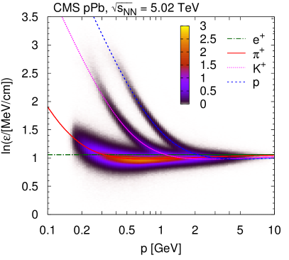
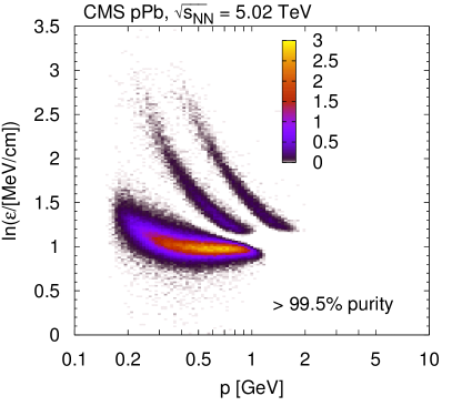
Figure 1: Logarithm of the most probable energy loss rate $\varepsilon$ normalized at a reference path length $l_{0}=450\mum$ in $\Pp$Pb collisions at $\sqrt{\smash[b]{s_{{}_{\text{NN}}}}}=5.02$. The distribution of $\ln\varepsilon$ is shown as a function of total momentum $p$ for positively charged particles (left), as well as for identified charged particles (both charges) with high purity selection ($>$ 99.5%, right). The linear $z$ axis scale is shown in arbitrary units. The curves show the expected $\ln\varepsilon$ for electrons, pions, kaons, and protons (full theoretical calculation, Eq. (33.11) in Ref. [23]).

0.3.2 Particle identification

The reconstruction of charged particles in CMS is limited by the acceptance of the tracker and by the decreasing tracking efficiency at low momentum. Particle-by-particle identification using specific ionization losses in the tracker is possible in the momentum range $p<0.15\GeV$ for electrons, $p<1.15\GeV$ for pions and kaons, and $p<2.00\GeV$ for protons (note that protons were not used for correlation studies in this analysis). In view of the $(\eta,\pt)$ regions where pions, kaons, and protons can all be identified, only particles in the range $-1<\eta<1$ (in the laboratory frame) are used for this measurement.

For the identification of charged particles, the estimated most probable energy loss rate $\varepsilon$ at a reference path length ($l_{0}=450\mum$) is used [24]. For an accurate determination of $\varepsilon$ and its variance $\sigma^{2}$ for each individual track, the responses of all readout chips in the tracker are calibrated with multiplicative gain correction factors. The procedures for gain calibration and track-by-track determination of $\varepsilon$ values are the same as in previous CMS analyses [16, 17].

Charged particles in the region $-1<\eta<1$ and $0<\pt<2\GeV$ are sorted into bins with a width of 0.1 units in $\eta$, and $0.05\GeV$ in $\pt$. Since the ratios of particle yields do not change significantly with the charged-particle multiplicity of the event [16, 17], the data are not subdivided into bins of $N_{\text{rec2}}$. The relative abundances of different particle species in a given $(\eta,\pt)$ bin are extracted by minimizing the joint log-likelihood

$$-2\ln{\mathcal{L}}=-2\sum_{i=\text{tracks}}\ln\left(\sum_{k=\Pgp,\PK,\Pp}P_{k}\exp\left[-\frac{(\ln\varepsilon_{i}-\mu_{k})^{2}}{2(\xi\sigma_{i})^{2}}\right]\right),$$ (1)

where $\mu_{k}$ are the expected means of $\ln\varepsilon$ for the different particle species, and $P_{k}$ are their relative probabilities. The value of $-2\ln{\mathcal{L}}$ is minimized by varying $P_{k}$ and $\mu_{k}$ starting from reasonable initial values. In the above formula $\varepsilon_{i}$ and $\sigma_{i}^{2}$ are the estimated most probable value and its estimated variance, respectively, for each individual track. Since the estimated variance can slightly differ from its true value, a scale factor $\xi$ is introduced. The $\mu_{k}$ values are used to determine a unique $\ln\varepsilon(p/m)$ function. A third-order polynomial closely approximates the collected $(p/m,\ln\varepsilon)$ pairs, within the corresponding uncertainties. This information is reused by fixing $\mu_{k}$ values according to the polynomial, and then re-determining $P_{k}$.

In this analysis a very high purity particle identification is achieved by requiring $P_{k}/(\sum_{k=\Pgp,\PK,\Pp}P_{k})>0.995$. If none of the particle type assumptions yields a $P_{k}$ value in this range, the particle is regarded as unidentified. This requirement ensures that less than 1% of the examined particle pairs are misidentified. The degree of purity achieved in particle identification is indicated by distributions of $\ln\varepsilon$ as a function of total momentum $p$ for $\Pp$Pb collisions at $\sqrt{\smash[b]{s_{{}_{\text{NN}}}}}=5.02$in Fig. 1. The left plot shows the initial distribution for positive particles. The plot for negatively charged particles is very similar. This distribution is compared to the theoretically expected energy loss for electrons, pions, kaons, and protons. In Fig. 1, the distribution of $\ln\varepsilon$ as a function of total momentum for identified charged particles with high purity is shown in the right plot. The plots for $\Pp\Pp$ and PbPb interactions are very similar.

0.4 The Bose–Einstein correlations

The correlation functions are investigated in one (1D), two (2D), and three (3D) dimensions in terms of $q_{\text{inv}}=\sqrt{(\vec{p}_{1}-\vec{p}_{2})^{2}-(E_{1}-E_{2})^{2}}$, as well as in projections of the relative three-momentum of the pair, $\vec{q}=\vec{p}_{1}-\vec{p}_{2}$, in two (in terms of longitudinal and transverse momenta, $q_{\text{L}}$, $q_{\text{T}}$), and three (in terms of out-short-long momenta, $q_{\text{L}}$, $q_{\text{S}}$, $q_{\text{O}}$) directions. In the center-of-mass (CM) frame the variables are defined as:

$$\vec{k}_{\mathrm{T}} =\frac{\vec{p}_{\text{T,1}}+\vec{p}_{\text{T,2}}}{2},$$

$$\vec{q}_{\mathrm{T}} =\vec{p}_{\mathrm{T,1}}-\vec{p}_{\mathrm{T,2}}, q_{\text{L}} =|p_{\mathrm{L,1}}-p_{\mathrm{L,2}}|$$

$$\vec{q}_{\mathrm{O}} =\left(\vec{q_{\text{T}}}\cdot\vec{e}_{\kt}\right)\vec{e}_{\kt}, \vec{q}_{\mathrm{S}} =\vec{q}_{\mathrm{T}}-\vec{q}_{\mathrm{O}}=\vec{e}_{\kt}\times\vec{q}_{\mathrm{T}},$$

where $\vec{e}_{\kt}\equiv\vec{k}_{\mathrm{T}}/\kt$ is a unit vector along the direction of the pair average transverse momentum, $\vec{k}_{\mathrm{T}}$. In the case of $\Pp\Pp$ collisions, and when dealing with the double ratio technique, the multidimensional investigations are carried out both in the CM frame and in the local co-moving system (LCMS). The latter is the frame in which the longitudinal component of the pair average momentum, $k_{\text{L}}=(k_{\text{L,1}}+k_{\text{L,2}})/2$, is zero. In the remainder of this paper, a common notation is used to refer to the magnitudes of the average and relative momentum vectors, $\kt=|\vec{k}_{\mathrm{T}}|$, $q_{\text{T}}=|\vec{q}_{\mathrm{T}}|$, $q_{\text{O}}=|\vec{q}_{\mathrm{O}}|$, and $q_{\text{S}}=|\vec{q_{\mathrm{S}}}|$.

0.4.1 Double ratio technique

The analysis procedure using the double ratio technique is the same as that described in Refs. [5, 6], where no particle identification is considered. However, the contamination by non-pions is expected to be small, since pions are the dominant type of hadrons in the sample (the ratio of kaons to pions is about 12%, and of protons to pions is roughly 6% [16]). The unidentified kaons and protons would contaminate mainly the low relative momentum region of the correlation functions. The impact of this level of contamination is covered by the systematic uncertainties.

For each event, the signal containing the BEC is formed by pairing same-sign tracks in the same event originating from the primary vertex, with $\abs{\eta}<2.4$ and $\pt>0.2\GeV$. The distributions in terms of the relative momentum of the pair (the invariant $q_{\text{inv}}$, or the components $q_{\text{T}}$, $q_{\text{L}}$ or $q_{\text{O}}$, $q_{\text{S}}$, $q_{\text{L}}$) are divided into bins of the reconstructed charged-particle multiplicity $N_{\text{trk0.4}}$, and of the pair average transverse momentum $\kt$. The distributions are determined in the CM and LCMS reference frames.

The background distribution or the reference sample can be constructed in several ways, most commonly formed by mixing tracks from different events (mixed-event technique), which can also be selected in several ways. In the first method employed in this analysis, the reference sample is constructed by pairing particles (all charge combinations) from mixed events and within the same $\eta$ range, as in Refs. [5, 6]. In this case, the full $\abs{\eta}<2.4$ interval is divided in three subranges: $-2.4<\eta<-0.8$, $-0.8\leq\eta<0.8$, and $0.8\leq\eta<2.4$. Alternative techniques considered for estimating the systematic uncertainties associated with this choice of reference sample are discussed in Sec. 0.4.5.

The correlation function is initially defined as a single ratio (SR), having the signal pair distribution as numerator and the reference sample as denominator, with the appropriate normalization,

$$\text{SR}(q)=C_{2}(q)=\left(\frac{\mathcal{N}_{\text{ref}}}{\mathcal{N}_{\text{sig}}}\right)\;\left(\frac{\text{d}N_{\text{sig}}/\text{d}q}{\text{d}N_{\text{ref}}/\text{d}q}\right),$$ (2)

where $C_{2}(q)$ is two-particle correlation function, $\mathcal{N}_{\text{sig}}$ is the integral of the signal content, whereas $\mathcal{N}_{\text{ref}}$ is the equivalent for the reference sample, both obtained by summing up the pair distributions for all the events in the sample. For obtaining the parameters of the BEC effect in this method, a double ratio (DR) is constructed [5, 6] as

$$\text{DR}(q)=\frac{\text{SR}(q)}{\text{SR}(q)_{\mathrm{MC}}}=\left[\left(\frac{\mathcal{N}_{\text{ref}}}{\mathcal{N}_{\text{sig}}}\right)\left(\frac{\rd{}N_{\text{sig}}/\rd{}q}{\rd{}N_{\text{ref}}/\rd{}q}\right)\right]\Big{/}\left[\left(\frac{\mathcal{N}_{\text{ref}}}{\mathcal{N}_{\text{sig}}}\right)_{\mathrm{MC}}\left(\frac{\rd{}N_{\mathrm{MC}}/\rd{}q}{\rd{}N_{\text{MC, ref}}/\rd{}q}\right)\right],$$ (3)

where $\text{SR}(q)_{\mathrm{MC}}$ is the single ratio as in Eq. (2), but computed with simulated events generated without BEC effects.

Since the reference samples in single ratios for data and simulation are constructed with exactly the same procedure, the bias due to such background construction could be, in principle, reduced when the DR is taken. However, even in this case, the correlation functions are still sensitive to the different choices of reference sample, leading to a spread in the parameters fitted to the double ratios, that is considered as a systematic uncertainty [5, 6]. On the other hand, by selecting MC tunes that closely describe the behavior seen in the data, this DR technique should remove the contamination due to non-Bose–Einstein correlations.

Table 0.4.1 shows the ranges and bin widths of relative momentum components used in fits to the double ratios. The bins in $\kt$ are also listed, which coincide with those in Refs. [5, 6].

Bin widths chosen for the various variables studied with the double ratio method. lcc Variable Bin ranges
$\kt$ [] 0.2–0.3, 0.3–0.5, 0.5–1.0
Range Bin width
$q_{\text{inv}}$  [] 0.02–2.0 $0.01{{}^{{}^{(*)}}}$/0.02
$q_{\text{T}}$, $q_{\text{L}}$  [] 0.02–2.0 0.05
$q_{\text{O}}$, $q_{\text{S}}$, $q_{\text{L}}$  [] 0.02–2.0 0.05
${}^{{}^{(*)}}$ for results integrated over $N_{\text{trk0.4}}$ and $\kt$ bins

0.4.2 Particle identification and cluster subtraction technique

Similarly to the case of unidentified particles discussed in Section 0.4.1, the identified hadron pair distributions are binned in the number of reconstructed charged particles $N_{\text{rec2}}$ of the event, in the pair average transverse momentum $\kt$, and also in the relative momentum variables in the LCMS of the pair in terms of $q_{\text{inv}}$, $(q_{\text{L}},q_{\text{T}})$ or $(q_{\text{L}},q_{\text{O}},q_{\text{S}})$. The chosen bin widths for pions and kaons are shown in Table 0.4.2.

Chosen bin widths for the various variables studied for pions and kaons in the particle identification and cluster subtraction method. lccc Variable Range Bin width

$N_{\text{rec2}}$ 0–240 10 60
 [] 0.2–0.7 0.1 0.1
$q_{\text{inv}}$ [] 0.0–2.0 0.02 0.04
$q_{\text{L}}$, $q_{\text{T}}$ [] 0.0–2.0 0.04 0.04
$q_{\text{L}}$, $q_{\text{O}}$, $q_{\text{S}}$ [] 0.0–2.0 0.04 0.04

The construction of the signal distribution is analogous to that described above: all valid particle pairs from the same event are taken and the corresponding distributions are obtained. Several types of pair combinations are used to study the BEC: , , , and ; while  and  are employed to correct for non-BEC contributions, as described in Section 0.4.3. For the reference sample an event mixing procedure is adopted, in which particles from the same event are paired with particles from 25 preceding events. Only events belonging to the same multiplicity ($N_{\text{rec2}}$) class are mixed. Two additional cases are also investigated. In one of them particles from the same event are paired, but the laboratory momentum vector of the second particle is rotated around the beam axis by 90 degrees. Another case considers pairs of particles from the same event, but with an opposite laboratory momentum vector of the second particle (mirrored). Based on the goodness-of-fit distributions of correlation function fits, the first event mixing prescription is used, while the rotated and mirrored versions, which give considerably worse $\chi^{2}/\mathrm{ndf}$ values, are employed in the estimation of the systematic uncertainty.

The measured two-particle correlation function $C_{2}(q)$ is itself the single ratio of signal and background distributions, as written in Eq. (2). This single ratio contains the BEC from quantum statistics, while non-BEC effects also contribute. Such undesired contributions are taken into account as explained in Section 0.4.3. A joint functional form combining all effects is fitted in order to obtain the radius parameter and the correlation function intercept, as discussed in Section 0.4.4.

0.4.3 Corrections for non-BEC effects

Effect of Coulomb interaction and correction

The BEC method employed for the study of the two-particle correlations reflects not only the quantum statistics of the pair of identical particles, but is also sensitive to final-state interactions. Indeed, the charged-hadron correlation function may be distorted by strong, as well as by Coulomb effects. For pions, the strong interactions can usually be neglected in femtoscopic measurements [25].

The Coulomb interaction affects the two-particle relative momentum distribution in a different way in the case of pairs with same-sign (SS) and opposite-sign (OS) electric charge. This leads to a depletion (enhancement) in the correlation function caused by repulsion (attraction) of SS (OS) charges. The effect of the mutual Coulomb interaction is taken into account by the factor $K$, the squared average of the relative wave function $\Psi$, as $K(q_{\text{inv}})=\int\rd^{3}\vec{r}\;f(\vec{r})\;|\Psi(\vec{k},\vec{r})|^{2}$, where $f(\vec{r})$ is the source intensity of emitted particles and $\vec{k}$ is the relative momentum of the pair. Pointlike sources, $f(\vec{r})=\delta(\vec{r})$, result in an expression for $K(q_{\text{inv}})$ coincident with the Gamow factor [26] which, in case of same sign and opposite sign charges, is given by

$$G^{\text{SS}}_{w}(\zeta)=|\Psi^{\text{SS}}(0)|^{2}=\frac{2\pi\zeta}{\re^{2\pi\zeta}-1},\qquad G^{\text{OS}}_{w}(\zeta)=|\Psi^{\text{OS}}(0)|^{2}=\frac{2\pi\zeta}{1-\re^{-2\pi\zeta}},$$ (4)

where $\zeta=\alpha m/q_{\text{inv}}$, is the Landau parameter, $\alpha$ is the fine-structure constant, $m$ is the particle mass, and $q_{\text{inv}}$ is the invariant relative momentum of the pair [27].

For extended sources, a more elaborate treatment is needed [28, 29], and the Bowler–Sinyukov formula [30, 25] is most commonly used. Although this does not differ significantly from the Gamow factor correction in the case of pions, this full estimate is required for kaons. The possible screening of Coulomb interaction, sometimes seen in data of heavy ion collisions [31, 32], is not considered. The value of zeta is typically $\zeta\ll 1$ in the $q$ range studied in this analysis. The absolute square of the confluent hypergeometric function of the first kind $F$, present in $\Psi$, can be approximated as $|F|^{2}\approx 1+2\zeta\operatorname{Si}(x)$, where $\operatorname{Si}$ is the sine integral function [33]. Furthermore, for Cauchy-type source functions ($f(r)=R/\{2\pi^{2}\left[r^{2}+(R/2)^{2}\right]^{2}\}$, where $f$ is normalized, such that $\int f(r)\,\rd^{3}r=1$), the Coulomb-correction factor $K$ is well described by the formula

$$K(q_{\text{inv}})=G_{w}(\zeta)\left[1+\pi\;\zeta\;q_{\text{inv}}R/(1.26+q_{\text{inv}}R)\right],$$ (5)

for $q_{\text{inv}}$ in $\GeV$, and $R$ in fm. The factor $\pi$ in the approximation comes from the fact that, for large $kr$ arguments, $\operatorname{Si}(kr)\to\pi/2$. Otherwise it is a simple but accurate approximation of the result of a numerical calculation, with deviations below 0.5%.

Clusters: mini-jets, multi-body decays of resonances

The measured opposite-sign correlation functions show contributions from various hadronic resonances [34]. Selected Coulomb-corrected correlation functions for low $N_{\text{rec2}}$ bins are shown in Fig. 2. The observed resonances include , , $\mathrm{f_{0}(980)}$, and $\mathrm{f_{2}(1270)}$ decaying to , and  decaying to . Photon conversions into  pairs, when misidentified as pion pairs, can also appear as a peak at very low $q_{\text{inv}}$ in the  spectrum. With increasing $N_{\text{rec2}}$ values the effect of resonances diminishes, since their contribution is quickly exceeded by the combinatorics of unrelated particles.

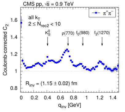
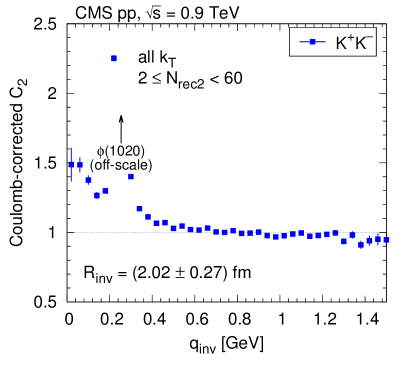
Figure 2: Contribution of resonance decays to the measured Coulomb-corrected correlation function of  (for $2\leq N_{\text{rec2}}<10$, left, blue squares) and  (for $2\leq N_{\text{rec2}}<60$, right, blue squares). The $\Pgf$ peak (right panel) is off-scale.

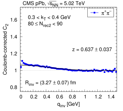
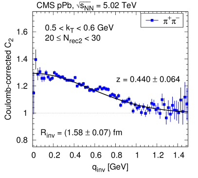
Figure 3: Contribution of clusters (mini-jets and multi-body decays of resonances) to the measured Coulomb-corrected correlation function of for $\Pp$Pb interactions at $\sqrt{\smash[b]{s_{{}_{\text{NN}}}}}=5.02$in two bins of event multiplicity and $\kt$. The solid curves show fits according to Eq. (6).

The Coulomb-corrected OS correlation functions are not always close to unity even at low $q_{\text{inv}}$, but show a Gaussian-like hump (Fig. 3). That structure has a varying amplitude with a stable scale ($\sigma$ of the corresponding Gaussian) of about 0.4. This feature is often related to particles emitted inside low-momentum mini-jets, but can be also attributed to the effect of multi-body decays of resonances. In the following we will refer to such an effect as due to fragmentation of clusters, or cluster contribution [35, 36, 37]. For the purpose of evaluating and later eliminating that contribution, the one-dimensional OS correlation functions are fitted with the following form:

$$C^{+-}_{2}(q_{\text{inv}})=c_{\text{OS}}\,K^{+-}(q_{\text{inv}})\;\left[1+\frac{b}{\sigma_{b}\sqrt{2\pi}}\exp\left(-\frac{q_{\text{inv}}^{2}}{2\sigma_{b}^{2}}\right)\right]$$ (6)

where $b$ and $\sigma_{b}$ are $N_{\text{rec2}}$- and -dependent parameters, and $c_{\text{OS}}$ is a normalization constant. The values of $b$ and $\sigma_{b}$ are parametrized using:

$$b(N_{\text{rec2}},\kt=\frac{b_{0}}{N_{\text{rec2}}^{n_{b}}}\exp\left(\frac{\kt}{k_{0}}\right),\qquad\sigma_{b}(N_{\text{rec2}},\kt)=\left[\sigma_{0}+\sigma_{1}\exp\left(-\frac{N_{\text{rec2}}}{N_{0}}\right)\right]\kt^{n_{\text{T}}}.$$ (7)

The amplitude $b$ is inversely proportional to a power of $N_{\text{rec2}}$ (with the exponent $n_{b}$ in the range 0.80–0.96). The parameter $b_{0}$ is much bigger for 5$\Pp$Pb than for 2.76PbPb data; for $\Pp\Pp$ collisions the dependence is described by $0.28\ln(\sqrt{s}/0.48\TeV)$. For $\Pp$Pb collisions $b_{0}$ is about 1.6–1.7 times higher than would be predicted from the $\Pp\Pp$ curve at the same $\sqrt{\smash[b]{s_{{}_{\text{NN}}}}}$. At the same time $b$ increases exponentially with , the parameter $k_{0}$ being in the range of 1.5–2.5. The Gaussian width $\sigma_{b}$ of the hump at low $q_{\text{inv}}$ first decreases with increasing $N_{\text{rec2}}$, but for $N_{\text{rec2}}>70$ remains constant at about 0.35–0.55. The width increases with $\kt$ as a power law, with the exponent $n_{\text{T}}$ in the range 0.19–0.33. The expression $b\sigma_{b}^{2}N_{\text{rec2}}$ is proportional to the fraction of particles that have a cluster-related partner. Our data show that this fraction does not change substantially with $N_{\text{rec2}}$, but increases with and $\sqrt{s}$ for $\Pp\Pp$ collisions. In summary, the object that generates this structure is assumed to always emit particles in a similar way, with a relative abundance that increases with the center-of-mass energy.

The cluster contribution can also be extracted in the case of the SS correlation function, if the momentum scale of the BEC effects and that of the cluster contribution ($\approx$0.4) are different enough. An important constraint in both mini-jet and multi-body resonance decays is the conservation of electric charge that results in a stronger correlation for OS pairs than for SS pairs. Consequently, the cluster contribution is expected to be present as well for SS pairs, with similar shape but a somewhat smaller amplitude. The form of the cluster-related contribution obtained from OS pairs, multiplied by a relative amplitude $z(N_{\text{rec2}},\kt)$ (ratio of measured OS to SS contributions), is used to fit the SS correlations. The dependence of this relative amplitude on $N_{\text{rec2}}$ in $\kt$ bins is shown in Fig. 4. Results (points with error bars) from all collision systems are plotted together with a parametrization ($(aN_{\text{rec2}}+b)/(1+aN_{\text{rec2}}+b)$) based on the combinatorics of SS and OS particle pairs (solid curves). Instead of the points, these fitted curves are used to describe the $N_{\text{rec2}}$ dependence of $z$ in the following. The $\pm$0.2 grey bands are chosen to cover most of the measurements and are used in determining a systematic uncertainty due to the subtraction of the cluster contribution.

Thus, the fit function for SS pairs is

$$C^{\pm\pm}_{2}(q_{\text{inv}})=c_{\text{SS}}\,K^{\pm\pm}(q_{\text{inv}})\;\left[1+z(N_{\text{rec2}})\frac{b}{\sigma_{b}\sqrt{2\pi}}\exp\left(-\frac{q_{\text{inv}}^{2}}{2\sigma_{b}^{2}}\right)\right]\;C_{\text{2,BE}}(q_{\text{inv}}),$$ (8)

where $K^{\pm\pm}$ describes the Coulomb effect, the squared brackets encompass the cluster contribution, and $C_{\text{2,BE}}(q_{\text{inv}})$ contains the quantum correlation to be extracted. Only the normalization $c_{\text{SS}}$ and the parameters of $C_{\text{2,BE}}(q_{\text{inv}})$ are fitted, all the other variables (those in $K^{\pm\pm}$, $z(N_{\text{rec2}})$, $b$, and $\sigma_{b}$) were fixed using Eq. (7).

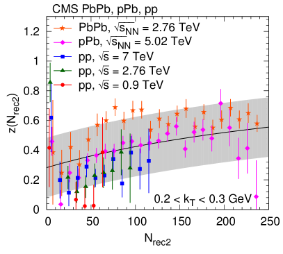
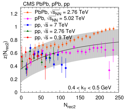
Figure 4: Dependence of the relative amplitude $z(N_{\text{rec2}})$ of the cluster contribution (between SS and OS pairs), as a function of $N_{\text{rec2}}$ for two $\kt$ bins. Fit results (points with error bars) from all collision types are plotted together with combinatorics-motivated fits (solid curves) and their estimated systematic uncertainties ($\pm$0.2 bands).

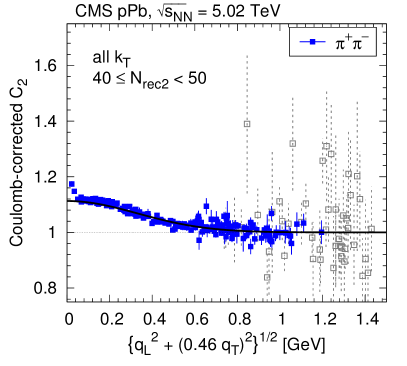
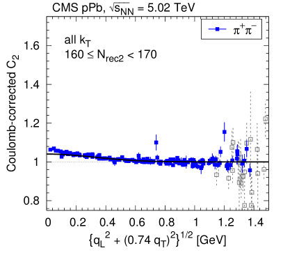
Figure 5: Coulomb-corrected OS correlation function of pions (blue squares) as a function of a combination of $q_{\text{L}}$ and $q_{\text{T}}$, in two selected $N_{\text{rec2}}$ bins for all $\kt$ values (left: $40\leq N_{\text{rec2}}<50$, right: $160\leq N_{\text{rec2}}<170$). For better visibility, only a randomly selected small fraction of the points is plotted. In addition, those with statistical uncertainty higher than 10% are plotted with light grey color. The solid curves indicate the prediction of the parametrized cluster contribution.

In the case of two and three dimensions, the measured OS correlation functions are constructed as a function of a length given by a weighted sum of $\vec{q}$ components, instead of $q_{\text{inv}}$. The Coulomb-corrected OS correlation functions of pions as a function of a combination of $q_{\text{L}}$ and $q_{\text{T}}$, $q_{h}=\sqrt{q_{\text{L}}^{2}+(aq_{\text{T}})^{2}}$, in selected $N_{\text{rec2}}$ bins for all , are shown in Fig. 5. The dependence of the $a$ factor on $N_{\text{rec2}}$ and is described by:

$$a(N_{\text{rec2}},\kt)=a_{0}-b_{0}\exp\left(-\frac{N_{\text{rec2}}}{N_{a}}-\frac{\kt}{k_{a}}\right).$$ (9)

This particular form is motivated by the physics results pointing to an elongated source, shown later in Section 0.6. The small peak at $q_{h}\approx 0$ is from photon conversions where both the electron and the positron are misidentified as a pion. The very low $q_{h}$ region is not included in the fits. Instead of the measurements, the fitted curves shown in Fig. 5 are used to describe the $N_{\text{rec2}}$ and $\kt$ dependence of these parameters in the following. Hence the fit function for SS pairs in the multidimensional case is:

$$C^{\pm\pm}_{2}(\vec{q})=c\,K^{\pm\pm}(q_{\text{inv}})\;\left[1+z(N_{\text{rec2}})\frac{b}{\sigma_{b}\sqrt{2\pi}}\exp\left(-\frac{q_{h}^{2}}{2\sigma_{b}^{2}}\right)\right]\;C_{\text{2,BE}}(\vec{q}).$$ (10)

In the formula above, only the normalization $c$ and the parameters of $C_{\text{2,BE}}(\vec{q})$ are fitted, all the other variables (those in $K^{\pm\pm}$, $z(N_{\text{rec2}})$, $b$, $\sigma_{b}$, and $a$) are fixed using the parametrization described above.

There are about two orders of magnitude less kaon pairs than pion pairs, and therefore a detailed study of the cluster contribution is not possible. We assume that their cluster contribution is similar to that of pions, and that the parametrization deduced for pions with identical parameters can be used (for $b$ and $\sigma_{b}$ in Eq. (7), and for $a$ in Eq. (9)). This choice is partly justified by OS kaon correlation functions shown later, but based on the observed difference, the systematic uncertainty on $z(N_{\text{rec2}})$ for kaons is increased to 0.3.

0.4.4 Fitting the correlation function

The parametrizations used to fit the correlation functions in 1D, 2D, and 3D in terms of $q_{\text{inv}}$, $(q_{\text{L}},q_{\text{T}})$, and $(q_{\text{S}},q_{\text{L}},q_{\text{O}})$, respectively, are the following [5, 6, 38]:

$$C_{\text{2,BE}}(q_{\text{inv}})=C[1+\lambda\re^{-(q_{\text{inv}}R_{\text{inv}})^{a}}]\,(1+\delta_{\text{inv}}\;q_{\text{inv}}),$$ (11)

is the fit function employed in the 1D case, while in the 2D case it has the form:

$$C_{\text{2,BE}}(q_{\text{T}},q_{\text{L}})=C\left\{1+\lambda\exp{\left[-\left|q_{\text{T}}^{2}R_{\text{T}}^{2}+q_{\text{L}}^{2}R_{\text{L}}^{2}+2q_{\text{T}}q_{\text{L}}R_{LT}^{2}\right|^{a/2}\right]}\right\}\,(1+\delta_{T}q_{\text{T}}+\delta_{L}q_{\text{L}}),$$ (12)

and, finally, the form used for 3D is:

$$C_{\text{2,BE}}(q_{\text{S}},q_{\text{L}},q_{\text{O}})= C\left\{1+\lambda\exp{\left[-\left|q_{\text{S}}^{2}R_{\text{S}}^{2}+q_{\text{L}}^{2}R_{\text{L}}^{2}+q_{\text{O}}^{2}R_{\text{O}}^{2}+2q_{\text{O}}q_{\text{L}}R_{\mathrm{LO}}^{2}\right|^{a/2}\right]}\right\}$$ (13)

$$\times(1+\delta_{S}q_{\text{S}}+\delta_{L}q_{\text{L}}+\delta_{O}q_{\text{O}}).$$

The radius parameters $R_{\text{inv}}$, $(R_{\text{T}},R_{\text{L}})$, $(R_{\text{S}},R_{\text{L}},R_{\text{O}})$, correspond to the lengths of homogeneity in 1D, 2D and 3D, respectively. In the above expressions, $\lambda$ is the intercept parameter (intensity of the correlation at $q=0$) and $C$ is the overall normalization. The polynomial factors on the right side, proportional to the fit variables $\delta_{\text{inv}},\delta_{T},\delta_{L},\delta_{S},\delta_{O}$, are introduced for accommodating possible deviations of the baseline from unity at large values of these variables, corresponding to long-range correlations. They are only used in the double ratio method, their values are uniformly set to zero in the case of the particle identification and cluster subtraction method that contains no such factors.

In Eq. (12), $R_{\text{T}}=R_{\text{T}}^{{}^{G}}+\tau\beta_{T}\cos\phi$ and $R_{\text{L}}=R_{\text{L}}^{{}^{G}}+\tau\beta_{L}$, where $R_{T,L}^{{}^{G}}$ are the geometrical transverse and longitudinal radii, respectively, whereas $\beta_{T}=\kt/k^{0}$ and $\beta_{L}=k_{\text{L}}/k^{0}$ are the transverse and longitudinal velocities, respectively; $\phi$ is the angle between the directions of $\vec{q}_{\mathrm{T}}$ and $\vec{k}_{\mathrm{T}}$, and $\tau$ is the source lifetime. Similarly, in Eq. (13) $R_{\text{S}}^{2}=(R_{S}^{{}^{G}})^{2}$, $R_{\text{L}}^{2}=(R_{L}^{{}^{G}})^{2}+\tau^{2}\beta_{L}^{2}$, $R_{\text{O}}^{2}=(R_{O}^{{}^{G}})^{2}+\tau^{2}\beta_{T}^{2}$, and $R_{LO}^{2}=\tau^{2}\beta_{L}^{2}\beta_{T}^{2}$ are the corresponding radius parameters in the 3D case. When the analysis is performed in the LCMS, the cross-terms $q_{\text{T}}q_{\text{L}}$ and $q_{\text{O}}q_{\text{L}}$ do not contribute for sources symmetric along the longitudinal direction.

Theoretical studies show that for the class of Lévy stable distributions (with index of stability $0<a\leq 2$) [38] the BEC function has a stretched exponential shape, corresponding to $a=1$ in Eqs. (12) and (13). This is to be distinguished from the simple exponential parametrization, in which the coefficients of the exponential would be given by $\sum_{i}R_{i}q_{i}$. In Section 0.5.3, the parameters resulting from the fits obtained with the simple and the stretched exponentials will be discussed in the 3D case. If $a$ is treated as a free parameter, it is usually between $a=1$ and $a=2$ (which corresponds to the Gaussian distribution [38]). In particular, for $a=1$, the exponential term in expressions given by Eqs. (12) and (13) coincides with the Fourier transform of the source function, characterized by a Cauchy distribution.

The measurements follow Poisson statistics, hence the correlation functions are fitted by minimizing the corresponding binned negative log-likelihood.

0.4.5 Systematic uncertainties

Double ratio method

Various sources of systematic uncertainties are investigated with respect to the double ratio results, similar to those discussed in Refs. [5, 6]: the MC tune used, the reference sample employed to estimate the single ratios, the Coulomb correction function, and the selection requirements applied to the tracks used in the analysis. From these, the major sources of systematic uncertainty come from the choice of the MC tune, followed by the type of reference sample adopted. In the latter case, alternative techniques to those considered in this analysis for constructing the reference sample are studied: mixing tracks from different events selected at random, taking tracks from different events with similar invariant mass to that in the original event (within 20%, calculated using all reconstructed tracks), as well as combining oppositely charged particles from the same event. Each of these procedures produces different shapes for the single ratios, and also leads to significant differences in the fit parameters. The exponential function in Eq. (11) (Lévy type with $a=1$) is adopted as the fit function in the systematic studies.

The results of the analysis do not show any significant dependence on the hadron charges, as obtained in a study separating positive and negative charges in the single ratios. Similarly, the effect of pileup, investigated by comparing the default results to those where only single-vertex events are considered, does not introduce an extra source of systematic uncertainty.

The sources of systematic uncertainties discussed above are considered to be common to $\Pp\Pp$ collisions at both 2.76 and 7. In the 1-D case the overall systematic uncertainty associated with $R_{\text{inv}}$ and that associated with $\lambda$ are estimated using the change in the fitted values found when performing the variations in procedure mentioned above for the four major sources of uncertainties at both energies. This leads to 15.5% and 10% for the systematic uncertainties in the fit radius and intercept parameters, respectively, which are considered to be common to all $N_{\text{trk}}$ and $\kt$ bins. The estimated values in the multidimensional cases were of similar order or smaller than those found in the 1-D case. Therefore, the systematic uncertainties found in the 1-D case were also applied to the 2-D and 3-D results.

Particle identification and cluster subtraction method

The systematic uncertainties are dominated by two sources: the construction of the background distribution, and the amplitude $z$ of the cluster contribution for SS pairs with respect to that for OS ones. Several choices for the construction of the background distribution are studied. The goodness-of-fit distributions clearly favor the event mixing prescription, while the rotated version gives poorer results, and the mirrored background yields the worst performance. The associated systematic uncertainty is calculated by performing the full analysis using the mixed event and the rotated variant, and calculating the root-mean-square of the final results (radii and $\lambda$).

Although the dependence of the ratio of the mini-jet contribution $z$ (between SS and OS pairs), as a function of $N_{\text{rec2}}$ could be well described by theory-motivated fits in all $\kt$ regions, the extracted ratios show some deviations within a given colliding system, and also between systems. In order to cover those variations, the analysis is performed by moving the fitted ratio up and down by 0.2 for pions, and by 0.3 for kaons. The associated systematic uncertainties are calculated by taking the average deviation of the final results (radii and $\lambda$) from their central values.

In order to suppress the effect of multiply-reconstructed particles and misidentified photon conversions, the low-$q$ region ($q<0.02\GeV$) is excluded from the fits. To study the sensitivity of the results to the size of the excluded range, its upper limit is doubled and tripled. Both the radii and $\lambda$ decreased slightly with increasing exclusion region. As a result, the contribution of this effect to the systematic uncertainty is estimated to be 0.1fm for the radii and 0.05 for $\lambda$.

The systematic uncertainties from all the sources related to the MC tune, Coulomb corrections, track selection, and the differences between positively and negatively charged particles are similar to those found in case of the double ratio method above. The systematic uncertainties from various sources are added in quadrature.

0.4.6 Comparisons of the techniques

In order to illustrate the level of consistency between both BEC analyses, the fit results for 1D $R_{\text{inv}}$ and $\lambda$ obtained employing the double ratio and the particle identification and cluster subtraction methods are compared. In the double ratio method, mixed events having similar multiplicities within the same $\eta$ ranges are used as the reference sample. The non-BEC effects are corrected with the double ratio technique, as discussed in Section 0.4.1, which also reduces the bias due to the choice of reference sample. In the particle identification and cluster subtraction method, single ratios are measured considering mixed pairs from 25 events chosen at random, whose contamination from resonance decays and mini-jet contributions are corrected as discussed in Sections 0.4.2 and 0.4.3. Regarding the final-state Coulomb corrections, no significant difference is observed if applying the Gamow factor, Eq. (4), or the full Coulomb correction, Eq. (5), to the correlation functions in $\Pp\Pp$ collisions. In both cases, the 1D correlations are fitted with an exponential function ($a=1$ in Eq. (11)), from which the radius and intercept parameters are obtained. Since in the particle identification and cluster subtraction method $\langle N_{\text{trk}}\rangle$ is fully corrected, as discussed in Section 0.3.1 and summarized in Table 0.3.1, an additional correction is applied to the values of $\langle N_{\text{trk0.4}}\rangle$ in Table 0.3.1 in the double ratio method, thus allowing the comparison of both sets of results plotted at the corresponding value of $\langle N_{\text{trk}}\rangle$. Such a correction is applied with a multiplicative factor obtained from the ratio of the total charged hadron multiplicities in both analyses, ${N_{\text{ch}}({\pt}\to 0)}/{N_{\text{ch}}({\pt}>0.4\GeV)}\sim 1.7$. The measurements are plotted in Fig. 6 for charged hadrons in the double ratio method and from identified charged pions from the particle identification and cluster subtraction method, as well as those for charged hadrons from Ref. [6]. In the latter, the correction factor is obtained in a similar fashion as ${N_{\text{ch}}({\pt}\to 0)}/{N_{\text{ch}}({\pt}>0.2\GeV)}\sim 1.1$, reflecting the $\pt>0.2\GeV$ requirement applied in that case.

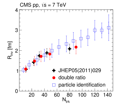
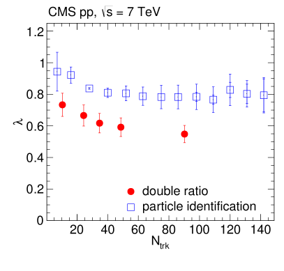
Figure 6: Dependence on track multiplicity of the radius (left) and intercept parameter (right), from the exponential fits to the 1D correlation functions via Eq. (11), obtained in the double ratio (filled markers) and the particle identification (for pions, empty squares) methods in $\Pp\Pp$ collisions at 7, together with the results from Ref. [6]. The inner (outer) error bars correspond to statistical (systematic) uncertainties.

The radius parameter $R_{\text{inv}}$ (Fig. 6, left) steadily increases with the track multiplicity. The results using the two different correlation techniques agree within the uncertainties, and they also agree well with our previous results [6]. In Fig. 6 (right), the corresponding results for the intercept parameter, $\lambda$, are shown integrated over all . The overall behavior of the correlation strength is again similar in both cases, showing first a decrease with $N_{\text{trk}}$ and then a flattening, approaching a constant for large values of the track multiplicity. The differences in the absolute values of the fit parameter $\lambda$ in the two approaches are related to the differences in $\pt$ (and $\kt$) acceptances for the tracking methods used in the two analyses, and the availability of particle identification, with both factors lowering the fit value of $\lambda$ for the double ratio method.

0.5 Results with the double ratio technique in collisions

0.5.1 One-dimensional results

Single and double ratios for $\Pp\Pp$ collisions at $\sqrt{s}=2.76$are shown in Fig. 7, integrated over the charged-particle multiplicity, $N_{\text{trk0.4}}$, and the pair momentum, $\kt$. The fit to the double ratio is performed using the exponential function in Eq. (11), with $a=1$. The corresponding fit values of the invariant radii, $R_{\text{inv}}$, and the intercept parameter, $\lambda$, are shown in Table 0.5.1, together with those for $\Pp\Pp$ collisions at $\sqrt{s}=7$; these being compatible within the uncertainties at these two energies.

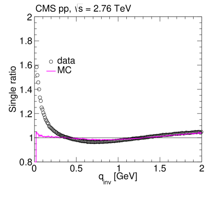
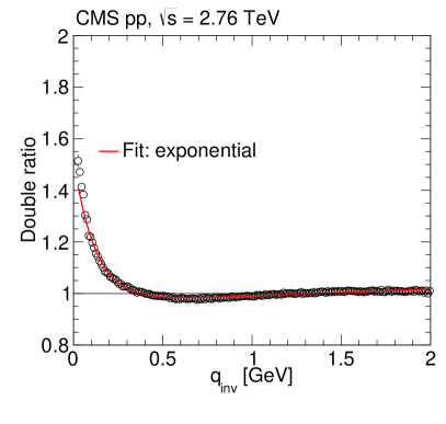
Figure 7: Left: 1D single ratios as a function of $q_{\text{inv}}$ for data and simulation (6 Z2 tune) in $\Pp\Pp$ collisions at $\sqrt{s}=2.76\TeV$. Right: Corresponding 1D double ratio versus $q_{\text{inv}}$ fitted to the superimposed exponential fit function. Only statistical uncertainties are included, commonly of the order or smaller than the marker size.

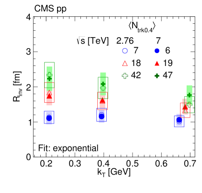
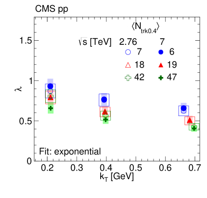
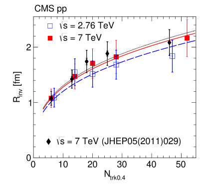
Figure 8: Top: $R_{\text{inv}}$(left) and $\lambda$ (right) as a function of $\kt$ obtained from an exponential fit to BEC data in three multiplicity bins in $\Pp\Pp$ collisions at 2.76(open symbols) and 7(filled symbols). The boxes indicate the systematic uncertainties. Bottom: Radius parameter $R_{\text{inv}}$ as a function of $N_{\text{trk0.4}}$ for $\Pp\Pp$ collisions at 2.76(open squares) and 7(filled squares), where the systematic uncertainties are shown as error bars and the statistical uncertainties are smaller than the marker size. Previous results at 7(filled diamonds) [6] are also shown, with their corresponding statistical (inner error bars) and statistical plus systematic uncertainties added in quadrature (outer error bars). The curves indicate the respective fits to a $N_{\text{trk0.4}}^{1/3}$ functional form.

Fit parameters of the 1D BEC function in $\Pp\Pp$ collisions at $\sqrt{s}=2.76$ and 7. lcc $\Pp\Pp$ $\sqrt{s}=2.76\TeV$ $\Pp\Pp$ $\sqrt{s}=7\TeV$
$\lambda$ $0.577\pm 0.007\stat\pm 0.058\syst$ $0.545\pm 0.001\stat\pm 0.054\syst$
$R_{\text{inv}}$ [fm] $1.624\pm 0.013\stat\pm 0.252\syst$ $2.022\pm 0.004\stat\pm 0.313\syst$

The upper panel of Fig. 8 shows the results for the invariant radius $R_{\text{inv}}$ (left) and the intercept parameter $\lambda$ (right), obtained with the exponential fit function in three bins of both $N_{\text{trk0.4}}$ and $\kt$, for $\Pp\Pp$ collisions at $\sqrt{s}=2.76$ and 7. The results corresponding to the two energies again show good agreement in the various ($N_{\text{trk0.4}}$, $\kt$) bins considered, extending the observation made with respect to the integrated values in Table 0.5.1 to different bin combinations of these variables. The parameter $\lambda$ decreases with increasing $\kt$, and its dependence on the charged multiplicity $N_{\text{trk0.4}}$ follows a similar trend. The fit invariant radius, $R_{\text{inv}}$, decreases with $\kt$, a behavior previously observed in several different collision systems and energy ranges [5, 6, 39, 40, 41, 42, 34], and expected for expanding emitting sources. In the case of heavy ion collisions, as well as for deuteron-nucleus and proton-nucleus collisions, both at the BNL RHIC and at the CERN LHC, this observed trend of the fit radii is compatible with a collective behavior of the source. The radius fit parameter is also investigated in Fig. 8 (bottom) for results integrated over $\kt$ bins and in five intervals of the charged-particle multiplicity, as in Table 0.3.1. The value of $R_{\text{inv}}$ steadily increases with multiplicity for $\Pp\Pp$ collisions at 2.76 and 7, as previously observed at 7in Ref. [6]. The various curves are fits to the data, and are proportional to $(N_{\text{trk0.4}})^{1/3}$, showing also that the results are approximately independent on the center-of-mass energy.

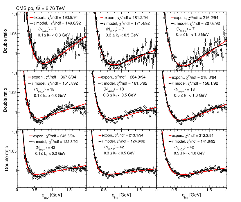
Figure 9: 1D correlation functions (with the $y$-axis cut off at $\sim$1.1) versus $q_{\text{inv}}$ obtained with the double ratio method in $\Pp\Pp$ at 2.76for increasing ranges of $\kt$ (left to right) and of $N_{\text{trk0.4}}$ (top to bottom). Data are fitted to the exponential (red curve) and the $\tau$ model (black curve) functions. The error bars show the statistical uncertainties.

As discussed in Ref. [6], the exponential fit alone in Eq. (11) is not able to describe the overall behavior of the correlation function in the range $0.2<q_{\text{inv}}<2\GeV$, for which an additional long-range term proportional to $q_{\text{inv}}$ is required. Although the general trend can be described by this parametrization, it misses the turnover of the baseline at large values of $q_{\text{inv}}$. The resulting poor fit quality is partially due to very small statistical uncertainties which restrict the variation of the parameters, but mainly due to the presence of an anticorrelation, i.e. correlation function values below the expected asymptotic minimum at unity, which is observed in the intermediate $q_{\text{inv}}$ range ($0.4<q_{\text{inv}}<1.1\GeV$). It is unlikely that this anticorrelation is due to the contamination of non-pion pairs in the sample, which would mainly give some contribution in the lower $q_{\text{inv}}$ region.

The anticorrelation depth depends on the range of $N_{\text{trk0.4}}$ considered, as reported in Ref. [6]. This is investigated further in this analysis by considering different $\kt$ bins for $\Pp\Pp$ collisions at 2.76 and 7. The results for the lower energy are shown in Fig. 9, where the data and the exponential fit are shown together with those based on Eq. (14). As previously observed in $\Pep\Pem$ collisions [43] and also in Ref. [6], this anticorrelation feature is compatible with effects as suggested by the $\tau$ model [44], where particle production has a broad distribution in proper time and the phase space distribution of the emitted particles is dominated by strong correlations of the space-time coordinate and momentum components. In this model the time evolution of the source is parameterized by means of a one-sided asymmetric Lévy distribution, leading to the fit function:

$$C_{\text{2,BE}}(q)=C\bigl{\{}1+\lambda\left[\cos\left[(qr_{0})^{2}+\tan(\nu\pi/4)(qr_{\nu})^{\nu}\right]\exp\{-(qr_{\nu})^{\nu}\}\right]\bigr{\}}\,(1+\delta\;q),$$ (14)

where the parameter $r_{0}$ is related to the proper time of the onset of particle emission, $r_{\nu}$ is a scale parameter entering in both the exponential and the oscillating factors, and $\nu$ corresponds to the Lévy index of stability.

The appearance of such anticorrelations may be due to the fact that hadrons are composite, extended objects. The authors of Ref. [45] propose a simple model in which the final-state hadrons are not allowed to interpenetrate each other, giving rise to correlated hadronic positions. This assumption results in a distortion in the correlation function, leading to values below unity.

Fitting the double ratios with Eq. (14) in the 1D case considerably improves the values of the $\chi^{2}/\mathrm{ndf}$ as compared to those fitted with the exponential function in Eq. (11), for $\Pp\Pp$ collisions at both 2.76 and 7 [6]. From Fig. 9, it can be seen that the fit based on Eq. (14) describes the overall behavior of the measurements more closely in all the bins of $N_{\text{trk0.4}}$ and $\kt$ investigated. In all but one of those bins, the fit based on the $\tau$ model results in $1<\chi^{2}/\text{ndf}<2$. In addition, a significant improvement is also observed when 2D and 3D global fits to the correlation functions are employed, mainly when the Lévy fit with $a=1$ is adopted (Sections 0.5.2 and 0.5.3).

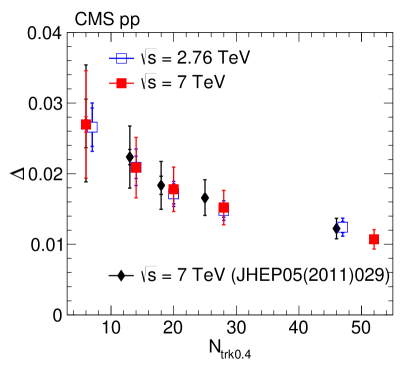
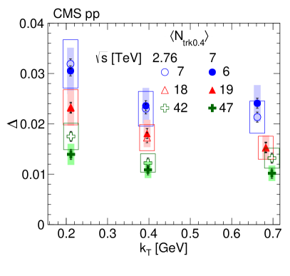
Figure 10: Left: Anticorrelation depth $\Delta$ as a function of $N_{\text{trk0.4}}$ integrated over all $\kt$, in $\Pp\Pp$ collisions at 2.76(open squares) and 7(filled squares), together with previous results at 7(filled diamonds) [6]. Inner (outer) error bars represent the statistical (plus systematic, added in quadrature) uncertainties. Right: Corresponding anticorrelation depth as a function of $\kt$ for various $N_{\text{trk0.4}}$ ranges, in $\Pp\Pp$ at 2.76(open symbols) and 7(filled symbols). The boxes indicate the systematic uncertainties.

The polynomial form $C(1+\delta\;q)$ in Eq. (14) is used as a baseline to quantify the depth of the dip [6]. This is estimated by the difference, $\Delta$, of the baseline function and the fit based on Eq. (14) at the minimum, leading to the results shown in Fig. 10. The left plot shows the present results for $\Pp\Pp$ collisions at 2.76 and at 7as a function of the multiplicity $N_{\text{trk0.4}}$ integrated over $\kt$ bins, exhibiting their consistency at different energies, as well as close similarity with the previous results [6]. The right plot in Fig. 10 shows the current results corresponding to the 2.76 and 7data further scrutinized in different $N_{\text{trk0.4}}$ and $\kt$ bins. From this plot, it can be seen that the depth of the dip decreases with increasing $N_{\text{trk0.4}}$ for both energies; however, the dependence on $\kt$ seems to decrease and then flatten out. In any case, the dip structure observed in the correlation function is a small effect, ranging from $\approx$3% in the lower $N_{\text{trk0.4}}$ and $\kt$ range investigated, to $\approx$1% in the largest one.

In summary, the BEC results obtained in $\Pp\Pp$ collisions and discussed in this section are shown to have a similar behavior to those observed in such systems in previous measurements at the LHC, by CMS [5, 6], as well as by the ALICE [46] and ATLAS [47] experiments. This behavior is reflected in the decreasing radii for increasing pair average transverse momentum $\kt$, and is also observed in $\Pep\Pem$ collisions at LEP [48]. Such behavior is compatible with nonstatic, expanding emitting sources. Correlations between the particle production points and their momenta, $(x,p)$ correlations, appear as a consequence of this expansion, generating a dependence of the correlation function on the average pair momentum, and no longer only on their relative momentum; $(x,p)$ correlations were modeled in Refs. [44, 45] as well. Similar behavior is also observed in various collision systems and energy ranges [5, 6, 39, 40, 41, 42, 34]. In the case of heavy ion, deuteron-nucleus, and proton-nucleus collisions, both at RHIC and at the LHC, these observations are compatible with a collective behavior of the source.

0.5.2 Two-dimensional results

The 1D analysis is extended to the 2D case in terms of the components ($q_{\text{T}},q_{\text{L}}$) of the pair relative momentum, for data samples at $\sqrt{s}=2.76$ and 7. In the 2D and 3D cases the measurement is conducted both in the CM frame and in the LCMS. For clarity, the asterisk symbol (*) is added to the variables defined in the CM frame when showing the results in this section. In the case of longitudinally symmetric systems, the LCMS has the advantage (Section 0.4.4) of omitting the cross-term proportional to $q_{\text{T}}q_{\text{L}}$ in the 2D, or $q_{\text{L}}q_{\text{O}}$ in the 3D fit functions.

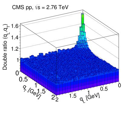
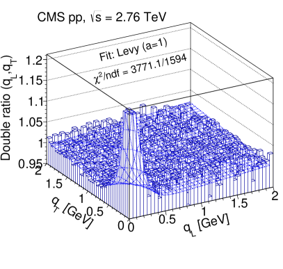
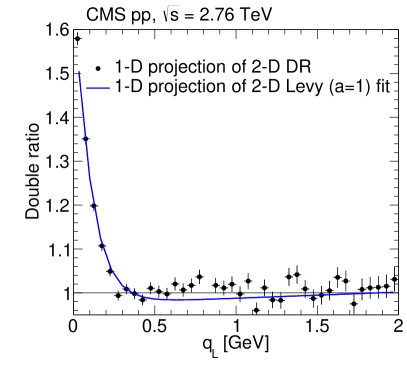
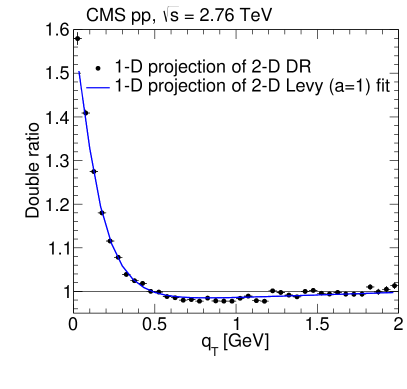
Figure 11: Double ratio results measured in the LCMS, integrated over all $N_{\text{trk0.4}}$ and $\kt$ bins, in $\Pp\Pp$ collisions at $\sqrt{s}=2.76\TeV$. Top: 2D correlation functions as a function of $(q_{\text{T}},q_{\text{L}})$ without (left) and with (right) the 2D Lévy (with $a=1$) fit function superimposed. Bottom: Corresponding 1D projections in terms of $q_{\text{L}}$ (for $q_{\text{T}}<0.05\GeV$, left) and $q_{\text{T}}$ (for $q_{\text{L}}<0.05\GeV$, right). The error bars indicate statistical uncertainties.

The 2D correlation function provides information on the behavior of the emitting source along and transverse to the beam direction. Typical examples are illustrated in Fig. 11 for $\Pp\Pp$ collisions at $\sqrt{s}=2.76\TeV$, in the LCMS. The upper panel shows the 2D plot of the double ratio in terms of $q_{\text{T}}$ and $q_{\text{L}}$, with the right plot showing the 2D Lévy fit (with $a=1$) defined in Eq. (12), superimposed on the 2D correlation function. The lower plots show 1D projections in terms of $q_{\text{L}}$ (left) and $q_{\text{T}}$ (right) of the 2D double ratios, and the corresponding 1D projections of the 2D Lévy (with $a=1$) fit function. When plotting in terms of $q_{\text{L}}$, only the first bin in $q_{\text{T}}$ (for $q_{\text{T}}<0.05\GeV$) is considered, and vice-versa. This choice is made to exhibit the largest values of the 2D correlation function in each direction, since the BEC decreases with increasing $q_{\text{T}},q_{\text{L}}$. The functions shown in the 1D figures are not fits to that data, but are projections of the global 2D-stretched exponential fit to the 2D correlation function. This explains the poor description of the data by the Lévy fit with $a=1$, in Fig. 11, left. The statistical uncertainties are also larger in the $q_{\text{L}}$ case, as well as the fluctuations in the results along this direction.

Analogously to the studies performed in 1D, the correlation functions are also investigated in 2D in terms of the components $(q_{\text{T}}^{(*)},q_{\text{L}}^{(*)})$, in three intervals of $\kt$, and in different $N_{\text{trk0.4}}$ bins. The results from the stretched exponential fit to the double ratios are compiled in Fig. 12, performed both in the CM frame (upper) and in the LCMS (lower). The behavior is very similar in both frames, clearly showing that all fit parameters $R_{\text{L}}^{(*)}$ and $R_{\text{T}}^{(*)}$ increase with increasing multiplicity $N_{\text{trk0.4}}$. On the other hand, the behavior with respect to $\kt$ varies, showing low sensitivity to this parameter for the lower $N_{\text{trk0.4}}$ bins. The radius parameters $R_{\text{L}}^{(*)}$ and $R_{\text{T}}^{(*)}$ decrease with $\kt$ for larger multiplicities, a behavior similar to that observed in the 1D case, and expected for expanding sources. The observation that $R_{\text{L}}\text{(LCMS)}>R_{\text{L}}^{*}\text{(CM)}$ for the same bins of $N_{\text{trk0.4}}$ and $\kt$ can be related to the Lorentz-contraction of the longitudinal radius in the CM frame.

Fit parameters of the 2D BEC function in $\Pp\Pp$ collisions at $\sqrt{s}=2.76$ and 7in the LCMS. lcc $\Pp\Pp$ $\sqrt{s}=2.76\TeV$ $\Pp\Pp$ $\sqrt{s}=7\TeV$
$\lambda$ $0.830\pm 0.010\stat\pm 0.083\syst$ $0.700\pm 0.002\stat\pm 0.070\syst$
$R_{\text{T}}$ [fm] $1.498\pm 0.013\stat\pm 0.232\syst$ $1.640\pm 0.003\stat\pm 0.254\syst$
$R_{\text{L}}$ [fm] $1.993\pm 0.022\stat\pm 0.309\syst$ $2.173\pm 0.006\stat\pm 0.337\syst$

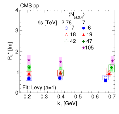
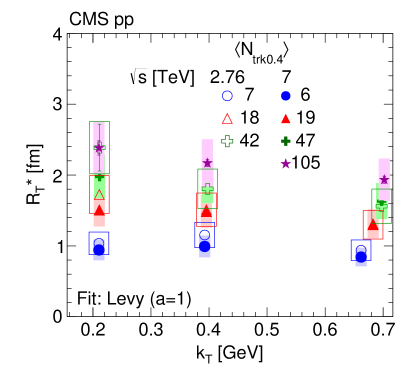
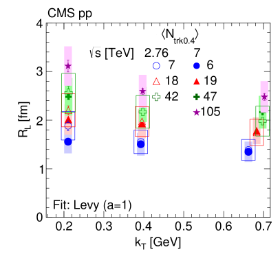
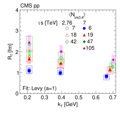
Figure 12: Radius parameters as a function of $\kt$, for different $N_{\text{trk0.4}}$ bins, obtained from data fitted to the stretched exponential function in $\Pp\Pp$ collisions at $\sqrt{s}=2.76\TeV$ (open symbols) and 7(filled symbols) in the CM frame (top) and in the LCMS (bottom). The boxes indicate the systematic uncertainties.

Figure 13 shows the results for the correlation strength parameter, $\lambda^{(*)}$, obtained with the same fit procedure, for both the CM and LCMS frames. No significant sensitivity of the intercept is seen as a function of $\kt$. However, within each $\kt$ range, $\lambda^{(*)}$ slowly decreases with increasing track multiplicity, in a similar way in both frames.

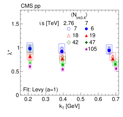
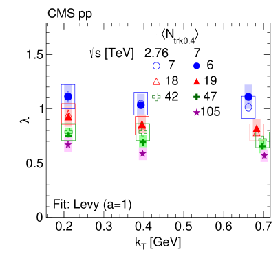
Figure 13: Intercept parameter $\lambda$ as a function of $\kt$, for different $N_{\text{trk0.4}}$ bins, obtained from data fitted to the stretched exponential function in $\Pp\Pp$ collisions at $\sqrt{s}=2.76\TeV$ (open symbols) and 7(filled symbols) in the CM frame (left) and in the LCMS (right). The boxes indicate the systematic uncertainties.

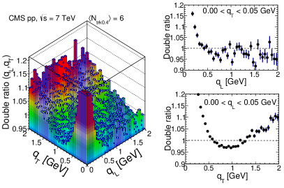
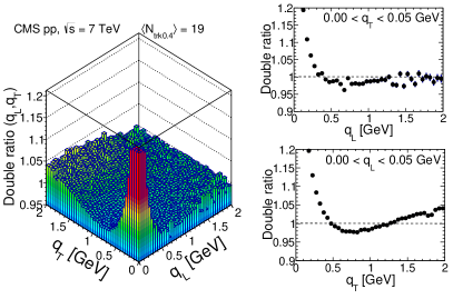
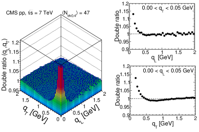
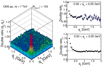
Figure 14: Results obtained in the LCMS for the 2D double ratios in the $(q_{\text{L}},q_{\text{T}})$ plane, zoomed along the correlation function axis, for four charged multiplicity bins, $N_{\text{trk0.4}}$ (integrated over all $\kt$), increasing from upper left to lower right. The BEC peak is cut off at $\sim$1.2 for a better visualization of the directional behavior. The 1D projections in $q_{\text{L}}$ (for $q_{\text{T}}<0.05\GeV$) and $q_{\text{T}}$ (for $q_{\text{L}}<0.05\GeV$) are shown to the right of the bidimensional plots, with error bars corresponding to statistical uncertainties.

The values obtained with the stretched exponential fit in the LCMS for the radius parameters $R_{\text{T}},R_{\text{L}}$, together with the intercept $\lambda$, corresponding to data integrated both in $N_{\text{trk0.4}}$ and $\kt$, are collected in Table 0.5.2 for $\Pp\Pp$ collisions at 2.76 and 7. The values fitted to the cross-term $R_{\text{LT}}$ in the CM frame are of order 0.5fm or less, and in the LCMS such terms are negligible ($\mathcal{O}[10^{-7}]$), as expected. From Table 0.5.2 it can be seen that, in the LCMS and at both energies, $R_{\text{L}}\approx 4R_{\text{T}}/3$, suggesting that the source is longitudinally elongated.

In Fig. 14 the 2D results for the double ratios versus ($q_{\text{L}},q_{\text{T}}$) in the LCMS are shown zoomed along the correlation function axis, with the BEC peak cut off around 1.2, for four charged-multiplicity bins, $N_{\text{trk0.4}}$. These plots illustrate the directional dependence of the $\kt$-integrated correlation functions along the beam and transverse to its direction, as well as the variation of their shapes when increasing the multiplicity range (from the upper left to the lower right plot) of the events considered. The edge effects seen for $q_{\text{T}}>1.5\GeV$ in the upper left plot (for $\langle N_{\text{trk0.4}}\rangle=6$) are an artifact of the cutoff at 1.2, being much smaller than the true value of the peak in the low ($q_{\text{L}},q_{\text{T}}$) region, and correspond to fluctuations in the number of pairs in those bins, due to a lower event count than in the other $N_{\text{trk0.4}}$ intervals. The $N_{\text{trk0.4}}$ ranges are the same as in Figs. 12–13, although the fit parameters shown in those figures are obtained considering differential bins in both $N_{\text{trk0.4}}$ and $\kt$. Figure 14 also shows the 1D projections of the 2D double ratios in terms of $q_{\text{T}}$ and $q_{\text{L}}$ (for values $q_{\text{L,T}}<0.05\GeV$). The shallow anticorrelation seen in the 1D double ratios in terms of $q_{\text{inv}}$ seems to be also present in the 2D plots, suggesting slightly different depths and shapes along the $q_{\text{L}}$ and $q_{\text{T}}$ directions.

0.5.3 Three-dimensional results

The double ratios can be further investigated in 3D as a function of the relative momentum components $(q_{\text{O}},q_{\text{S}},q_{\text{L}})$. In order to obtain the corresponding fit parameters, $(R_{\text{O}},R_{\text{S}},R_{\text{L}})$, as well as the correlation function strength, $\lambda$, the fits are performed to the full 3D double ratios and, if desired for illustration purposes, projected onto the directions of the variables $q_{\text{O}},q_{\text{S}},q_{\text{L}}$, similarly to the projections done for the measurements. The 3D correlation functions can be visualized through 2D projections in terms of the combinations $(q_{\text{S}},q_{\text{L}})$, $(q_{\text{L}},q_{\text{O}})$, and $(q_{\text{O}},q_{\text{S}})$, with the complementary components constrained to $q_{\text{O}}<0.05\GeV$, $q_{\text{S}}<0.05\GeV$, and $q_{\text{L}}<0.05\GeV$, respectively, corresponding to the first bin in each of these variables. For clarity, the asterisk symbol (*) is added to the variables defined in the CM frame when showing the results in this section. An illustration of the 2D projections is shown in the upper panel of Fig. 15, with data from $\Pp\Pp$ collisions at 7, integrated in all $N_{\text{trk0.4}}$ and $\kt$ ranges. Similarly to Fig. 14, the results are zoomed along the 3D double ratio axis, with the BEC peak cut off around 1.2 for better visualization of the directional behavior of the correlation function. The higher values seen around $(q_{\text{O}},q_{\text{S}})\sim(2,2)\GeV$ in the upper middle plot are again artifacts of cutting the double ratio at 1.2, this value being much smaller than the true value of the peak in the low ($q_{\text{O}},q_{\text{S}}$) region, and correspond to fluctuations in the number of pairs in those bins.

The lower panel in Fig. 15 shows the corresponding 1D projections of the full 3D correlation function and fits. Similarly to what was stressed regarding Fig. 11, the functions shown in Fig. 15 are projections of the global 3D-stretched exponential fit to the 3D correlation function. This explains the poor description of the 1D data by the Lévy fit with $a=1$.

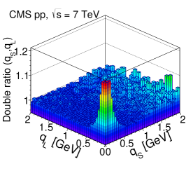
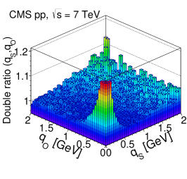
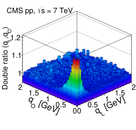
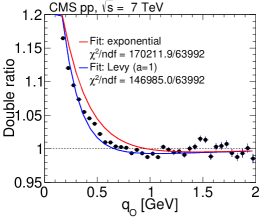
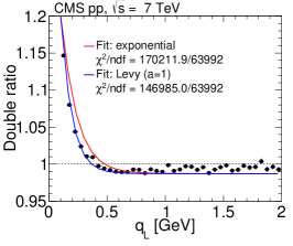
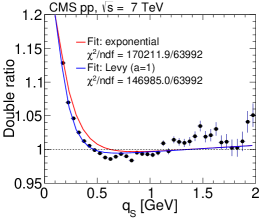
Figure 15: Results obtained in the LCMS for the 3D double ratios in $\Pp\Pp$ collisions at 7, integrated over $N_{\text{trk0.4}}$ and $\kt$. Top: 2D projections over the $(q_{\text{L}},q_{\text{S}})$, $(q_{\text{O}},q_{\text{S}})$, and $(q_{\text{O}},q_{\text{L}})$ planes, for $q_{\text{O}}<0.05\GeV$ (left), $q_{\text{L}}<0.05\GeV$ (middle), and $q_{\text{S}}<0.05\GeV$ (right). Bottom: 1D projections of the same data, with the complementary two variables constrained to be within the first bin ($q_{i,j}<0.05\GeV$). The error bars show the corresponding statistical uncertainties. All plots are zoomed along the correlation function axis with the BEC peak cut off above 1.2.

The values of the radii in the Bertsch–Pratt parametrization [49, 50] for $\Pp\Pp$ collisions at both 2.76 and 7, obtained with the stretched exponential fit in the LCMS and integrating over all $N_{\text{trk0.4}}$ and $\kt$ ranges, are summarized in Table 0.5.3, together with the corresponding intercept fit parameter.

Parameters of the 3D BEC function, obtained from a stretched exponential fit, in $\Pp\Pp$ collisions at $\sqrt{s}=2.76$ and 7in the LCMS. lcc $\Pp\Pp$ $\sqrt{s}=2.76\TeV$ $\Pp\Pp$ $\sqrt{s}=7\TeV$
$\lambda$ $0.799\pm 0.001\stat\pm 0.080\syst$ $0.679\pm 0.002\stat\pm 0.068\syst$
$R_{\text{O}}$ [fm] $1.129\pm 0.016\stat\pm 0.175\syst$ $1.256\pm 0.003\stat\pm 0.195\syst$
$R_{\text{S}}$ [fm] $1.773\pm 0.017\stat\pm 0.275\syst$ $1.842\pm 0.004\stat\pm 0.286\syst$
$R_{\text{L}}$ [fm] $2.063\pm 0.022\stat\pm 0.320\syst$ $2.120\pm 0.004\stat\pm 0.329\syst$

Comparing the LCMS radii in the 3D case for $\Pp\Pp$ collisions at 7, the hierarchy $R_{\text{L}}>R_{\text{O}}$ and $R_{\text{L}}\gtrsim R_{\text{S}}$ can be seen (although the values of $R_{\text{L}}$ and $R_{\text{S}}$ are also compatible with each other within their statistical and systematic uncertainties). Therefore, as in the 2D case, the 3D source also seems to be more elongated along the longitudinal direction in the LCMS, with the relationship between the radii being given by $R_{\text{L}}\gtrsim R_{\text{S}}>R_{\text{O}}$. A similar inequality holds for $\Pp\Pp$ collisions at 2.76.

The data sample obtained in $\Pp\Pp$ collisions at 2.76in 2013 is considerably smaller than at 7and would lead to large statistical uncertainties if the double ratios in the 3D case are measured differentially in $N_{\text{trk0.4}}$ and $\kt$, so this study is not considered at 2.76.

For the data from $\Pp\Pp$ collisions at 7, the fits to the double ratios are investigated in three bins of the pair average transverse momentum, $\kt$ (integrating over charged multiplicity, $N_{\text{trk0.4}}$). The fit parameters are obtained with exponential and Lévy (with $a=1$) type functions. The corresponding results are compiled in Fig. 16, both in the CM frame and in the LCMS, showing that the values are very sensitive to the expression adopted for the fit function, as also suggested in Fig. 15 by the 1D projections of the global 3D fit performed to the 3D double ratios.

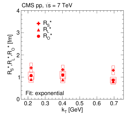
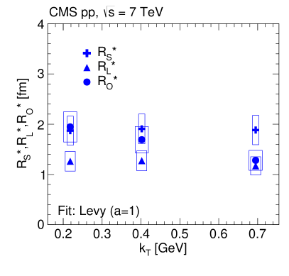
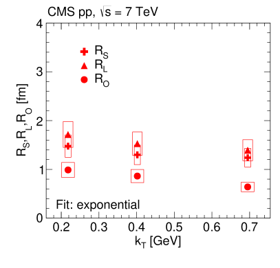
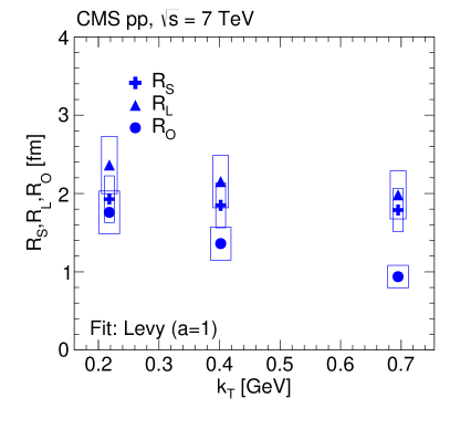
Figure 16: 3D radii parameters as a function of $\kt$ (integrated over all $N_{\text{trk0.4}}$), obtained from double ratios fitted to the exponential (left) and Lévy (with $a=1$, right) functions for $\Pp\Pp$ collisions at $\sqrt{s}=7$in the CM frame (top) and in the LCMS (bottom). The boxes indicate the systematic uncertainties.

In the LCMS, the behavior of $R_{\text{S}}$ with increasing pair average transverse momentum is very similar to that of $R_{\text{S}}^{*}$ in the CM frame, and the fit values are consistent within statistical and systematic uncertainties, as would be expected, since the boost to the LCMS is in the longitudinal direction. It can also be seen in both frames that the sideways radius is practically independent of $\kt$, within the uncertainties. The outwards fit parameter $R_{\text{O}}^{(*)}$ shows a similar decrease with respect to $\kt$ in both frames. However, in the CM frame the $R_{\text{O}}^{*}$ fit values are slightly larger than those in the LCMS ($R_{\text{O}}$) for the same ($N_{\text{trk0.4}},\kt$) bins. This is compatible with the dependence of $R_{\text{O}}^{(*)}$ on the source lifetime (as seen in Section 0.4.4), which is expected to be higher in the CM frame than in the LCMS, because of the Lorentz time dilation. In the LCMS, $R_{\text{L}}$ decreases with increasing $\kt$. It has larger values than in the CM frame for both energies, suggesting an effect related to the Lorentz boost, similar to the 2D case. Also in this frame, its decrease with increasing $\kt$ is more pronounced for the same reason.

The fits to the double ratios are also studied in four bins of $N_{\text{trk0.4}}$ integrating over all $\kt$, and the corresponding results are shown in Fig. 17, both in the CM frame (upper) and in the LCMS (lower). A clear trend can be seen, common to both fit functions and in all directions of the relative momentum components: the radii $R_{\text{S}}^{(*)}$, $R_{\text{L}}^{(*)}$, and $R_{\text{O}}^{(*)}$ increase with increasing average multiplicity, $N_{\text{trk0.4}}$, similar to what is seen in the 1D and 2D cases.

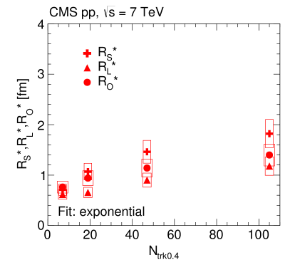
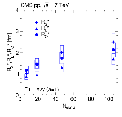
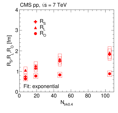
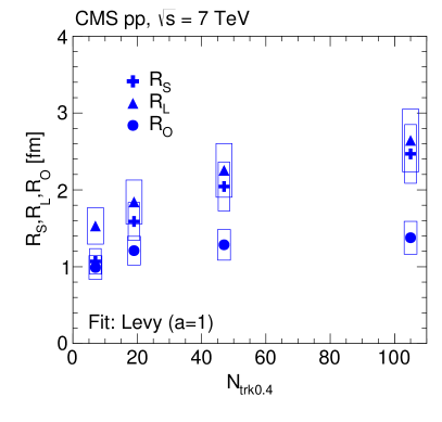
Figure 17: 3D radii parameters as a function of $N_{\text{trk0.4}}$ (integrated over all $\kt$), obtained from double ratios fitted to the exponential (left) and Lévy (with $a=1$, right) functions for $\Pp\Pp$ collisions at $\sqrt{s}=7$in the CM frame (top) and in the LCMS (bottom). The boxes indicate the systematic uncertainties.

The intercept parameter $\lambda^{(*)}$ is also studied as a function of $\kt$ and $N_{\text{trk}}$, both in the CM frame and in the LCMS. The corresponding results are shown in Fig. 18. A moderate decrease with increasing $\kt$ is observed. As a function of $N_{\text{trk0.4}}$, $\lambda^{(*)}$ first decreases with increasing charged-particle multiplicity and then it seems to saturate.

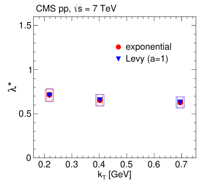
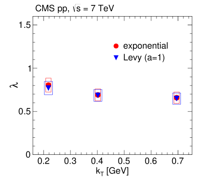
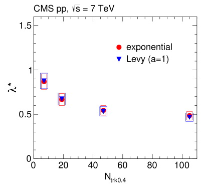
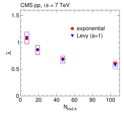
Figure 18: Intercept parameter $\lambda^{(*)}$ in the CM frame (left) and in the LCMS (right) as functions of $\kt$ (integrated over $N_{\text{trk0.4}}$, top) and of $N_{\text{trk0.4}}$ (integrated over $\kt$, bottom), obtained from fits to the double ratios with the exponential and the Lévy (with $a=1$) functions in $\Pp\Pp$ collisions at 7. The boxes indicate the systematic uncertainties.

Since the longitudinal radius parameter represents the same length of homogeneity along the beam direction, it would be expected that the corresponding fit values in the 2D and 3D cases are comparable. In fact, they are consistent within the experimental uncertainties, as can be seen in Fig. 19, except in the first bin of $N_{\text{trk0.4}}$ investigated in the CM frame, where the central $R_{\text{L}}$ value in 3D is roughly 0.3fm larger than the corresponding $R_{\text{L}}$ value in 2D, for $\Pp\Pp$ collisions at both 2.76 and 7. This difference, however, may reflect a better description of the source in the 3D case, where the transverse component is decomposed into two independent orthogonal directions, whereas it may not be fully accommodated by considering just one transverse parameter as in the 2D case. In addition, it can be seen in Fig. 19 that there is an approximate energy independence of $R_{\text{L}}^{*}$ ($R_{\text{L}}$) as a function of $N_{\text{trk0.4}}$, for results at $\sqrt{s}=2.76$ and 7, similar to what is observed in the 1D case.

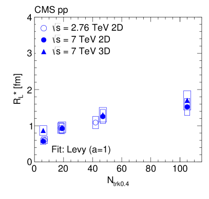
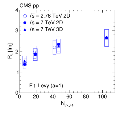
Figure 19: Longitudinal radius parameter as a function of $N_{\text{trk0.4}}$ (integrated over all $\kt$) in the CM frame ($R_{\text{L}}^{*}$, left) and in the LCMS ($R_{\text{L}}$, right), obtained from 2D correlation functions fitted as functions of $q_{\text{T}}$ and $q_{\text{L}}$, compared to the values obtained in the 3D case (fits as a function of $q_{\text{S}}$, $q_{\text{L}}$, and $q_{\text{S}}$), in $\Pp\Pp$ collisions at $\sqrt{s}=2.76$(open symbols) and 7(closed symbols). The boxes indicate the systematic uncertainties.

0.6 Results with particle identification and cluster subtraction in , $\Pp$Pb, and PbPb collisions

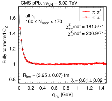
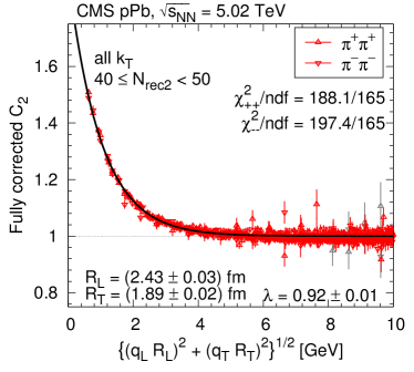
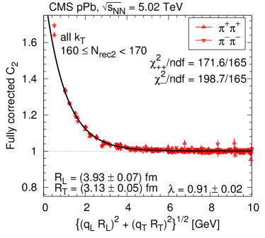
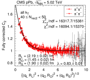
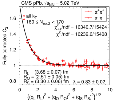
Figure 20: SS correlation function (integrated over all $\kt$) measured in $\Pp$Pb collisions at 5.02as a function of $q_{\text{inv}}$ or of the combined momentum, in two selected $N_{\text{rec2}}$ bins (left and right), for pion pairs (red triangles) in one (top), two (middle), and three (bottom) dimensions, corrected for Coulomb interaction and cluster contributions (mini-jets and multi-body resonance decays). For better visibility, only a fraction of the points is plotted, and those with statistical uncertainty higher than 10% are in light-grey color. The solid curves indicate fits with the stretched exponential parametrization.

A selection of correlation functions obtained using the mixed-event prescription, as described in Section 0.4.2, and the corresponding fits are shown in Figs. 20 (pions) and 21 (kaons). The SS correlation functions, corrected for Coulomb interaction and cluster contribution (mini-jets and multi-body resonance decays), as a function of $q_{\text{inv}}$, $(q_{\text{L}},q_{\text{T}})$, and $(q_{\text{L}},q_{\text{O}},q_{\text{S}})$ in selected $N_{\text{rec2}}$ bins are plotted for all . The solid curves indicate fits with the stretched exponential parametrization. Although the probability of reconstructing multiple tracks from a single true track is very small (about 0.1%), the bin with the smallest $|\vec{q}|$ is not used in the fits in order to avoid regions potentially containing pairs of multiply-reconstructed tracks.

The fits are mostly of good quality, the corresponding $\chi^{2}/\mathrm{ndf}$ values being close to one in the 2D and 3D cases, for pions and kaons alike. The stretched exponential parametrization provides an excellent match to the data. The 1D correlation function shows a wide minimum around 0.5(Fig. 20, upper panel). The amplitude of that very shallow dip is of the order of a few percent only, and is compatible with the previously discussed results.

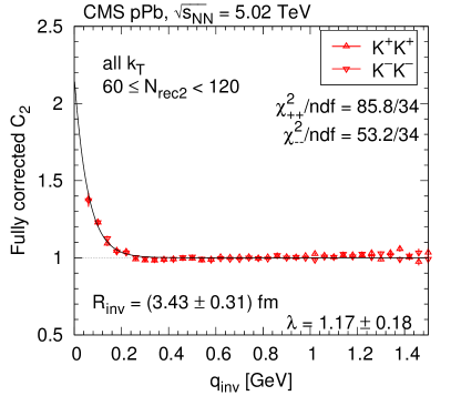
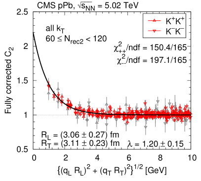
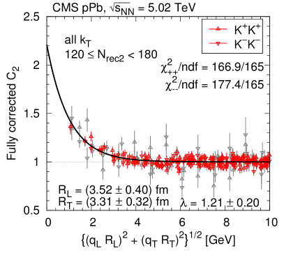
Figure 21: SS correlation function (integrated over all $\kt$) measured in $\Pp$Pb collisions at 5.02as a function of $q_{\text{inv}}$ or of the combined momentum, in two selected $N_{\text{rec2}}$ bins (left and right), for kaon pairs (red triangles) in one (top) and two (bottom) dimensions, corrected for Coulomb interaction and cluster contributions (mini-jets and multi-body resonance decays). For better visibility, only a fraction of the points is plotted, and those with statistical uncertainty higher than 10% are in light-grey color. The solid curves indicate fits with the stretched exponential parametrization.

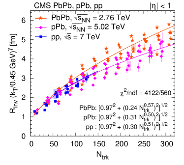
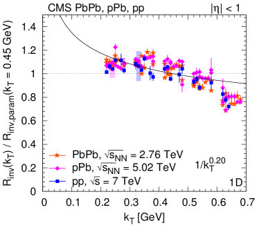
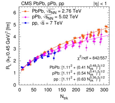
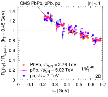
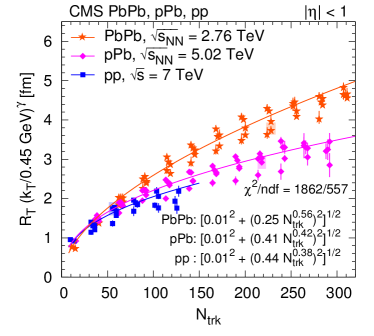
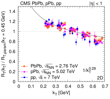
Figure 29: Left: Radius parameters for pions as a function of $N_{\text{trk}}$ scaled to $\kt=0.45\GeV$ with help of the parametrization, as $R(\kt/0.45\GeV)^{\gamma}$ (Eq. (15)). Right: Ratio of the radius parameter and the value of the parametrization $R_{\text{param}}$ (Eq. (15)) at $\kt=0.45\GeV$ as a function $\kt$. (For better visibility, points are shifted to left and to right with respect to the center of the $\kt$ bin. Systematic uncertainties are indicated with shaded boxes, only for a fraction of the points.) Upper row: $R_{\text{inv}}$ from the 1D ($q_{\text{inv}}$) analysis. Middle row: $R_{\text{L}}$ from the 2D $(q_{\text{L}},q_{\text{T}})$ analysis. Lower row: $R_{\text{T}}$ from the 2D $(q_{\text{L}},q_{\text{T}})$ analysis. Fit results are indicated in the figures, see text for details.

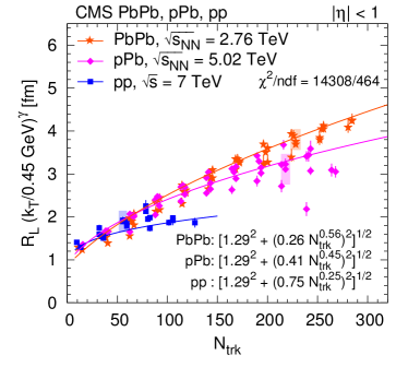
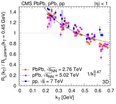
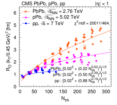
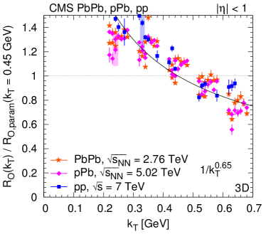
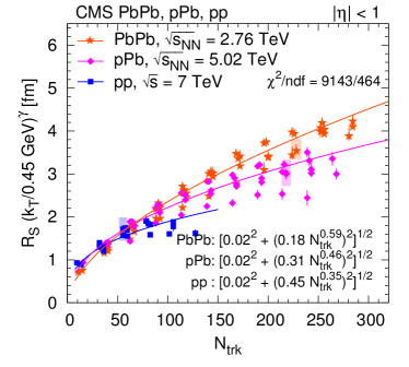
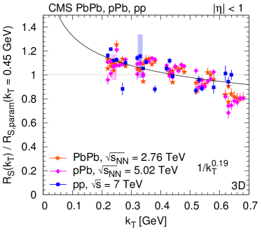
Figure 30: Left: Radius parameters for pions as a function of $N_{\text{trk}}$ scaled to $\kt=0.45\GeV$ with help of the parametrization as $R(\kt/0.45\GeV)^{\gamma}$ (Eq. (15)). Right: Ratio of the radius parameter and the value of the parametrization $R_{\text{param}}$ (Eq. (15)) at $\kt=0.45\GeV$ as a function $\kt$. (For better visibility, points are shifted to left and to right with respect to the center of the $\kt$ bin. Systematic uncertainties are indicated with shaded boxes, only for a fraction of the points.) Radii from the 3D $(q_{\text{L}},q_{\text{O}},q_{\text{S}})$ analysis are shown, from upper to lower: $R_{\text{L}}$, $R_{\text{O}}$, $R_{\text{S}}$. Fit results are indicated in the figures, see text for details.

The characteristics of the extracted one-, two-, and three-dimensional correlation functions of identified pions and kaons in $\Pp\Pp$, $\Pp$Pb, and peripheral PbPb collisions are presented in Figs. 22–30 as functions of the pair average transverse momentum $\kt$ and of the corrected charged-particle multiplicity $N_{\text{trk}}$ of the event (in the range $\abs{\eta}<2.4$ in the laboratory frame, with integrated results extrapolated to $\pt=0$). In all plots, the results of positively and negatively charged pions and kaons are averaged. The central values for the radii and intercept parameter $\lambda$ are given by markers. The statistical uncertainties are indicated by vertical error bars, while the combined systematic uncertainties (choice of background method; uncertainty in the relative amplitude $z$ of the cluster contribution; low $q$ exclusion) are given by the filled boxes. Unless indicated, the lines are drawn to guide the eye (cubic splines whose coefficients are found by weighting the measurements with the inverse of their squared statistical uncertainty).

0.6.1 Dependencies on $N_{\text{trk}}$ and $\kt$

The $N_{\text{trk}}$ dependence of the 1D radius $R_{\text{inv}}$ and intercept $\lambda$ parameters for pions (Eq. (8)), averaged over several bins, for all studied systems are shown in Fig. 22. The radii found for pions from $\Pp\Pp$ collisions span a similar range to those found previously [5, 6], as well as those obtained for charged hadrons via the double ratio technique, as reported in Section 0.5.1. Although illustrated in Fig. 22 for the -integrated case only, the dependence on the number of tracks of the 1D pion radius parameter is remarkably similar for $\Pp\Pp$ and $\Pp$Pb collisions in all bins. This also applies to PbPb collisions when $\kt>0.4\GeV$. The values of the pion intercept parameter $\lambda$ are usually below unity, in the range 0.7–1, and seem to remain approximately constant as a function of $N_{\text{trk}}$ for all systems and $\kt$ bins. Similar results obtained for kaons in the 1D analysis are displayed in Fig. 23. The 1D kaon radius parameter increases with $N_{\text{trk}}$, but with a smaller slope than seen for pions.

The dependencies of the 1D radius parameters for pions, in several $N_{\text{trk}}$ bins for the $\Pp\Pp$ and $\Pp$Pb systems are plotted in Fig. 24. They show a decrease with increasing $\kt$ for $\kt>0.4\GeV$.

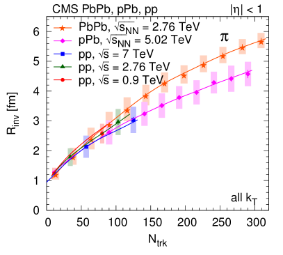
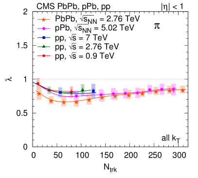
Figure 22: Track-multiplicity ($N_{\text{trk}}$) dependence of the 1D pion radius parameter $R_{\text{inv}}$ (left) and intercept parameter $\lambda$ (right), obtained from 1D fits (integrated over all $\kt$) for all collision systems studied. For better visibility, only every second measurement is plotted. Lines are drawn to guide the eye.

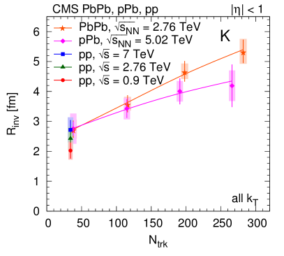
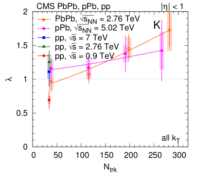
Figure 23: Track-multiplicity ($N_{\text{trk}}$) dependence of the 1D kaon radius parameter $R_{\text{inv}}$ (left) and intercept parameter $\lambda$ (right), obtained from 1D fits (integrated over all $\kt$) for all collision systems studied. For better visibility, only every second measurement is plotted. Lines are drawn to guide the eye.

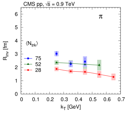
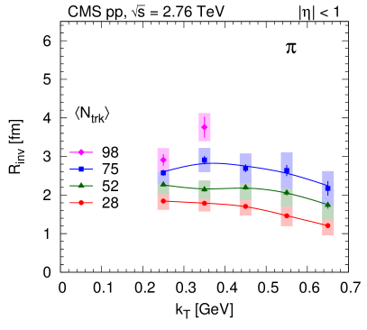
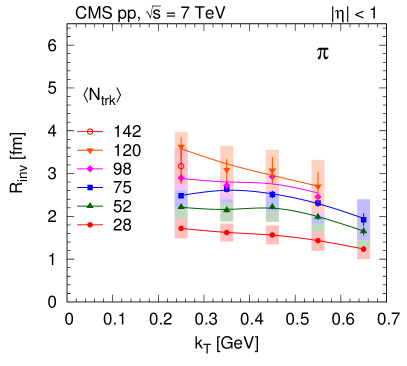
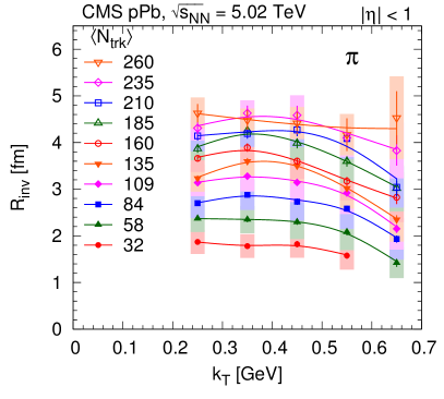
Figure 24: $\kt$-dependence of the 1D pion radius $R_{\text{inv}}$, for several $N_{\text{trk}}$ bins, extracted for the $\Pp\Pp$ and $\Pp$Pb systems. Lines are drawn to guide the eye.

The $N_{\text{trk}}$ dependence of the 2D radii and the corresponding intercept parameters for pions (Eq. (10)), in several bins, for all studied systems are shown in Fig. 25. The $N_{\text{trk}}$ dependence of 2D pion radius parameters, $R_{\text{L}}$ and $R_{\text{T}}$, is similar for $\Pp\Pp$ and $\Pp$Pb collisions in all bins. In general $R_{\text{L}}>R_{\text{T}}$, indicating that the source is elongated in the beam direction, a behavior also seen in $\Pp\Pp$ collisions with the double ratio technique, as discussed in Section 0.5.1. In the case of PbPb collisions $R_{\text{L}}\approx R_{\text{T}}$, indicating that the source is approximately symmetric. In the case of kaons, the results corresponding to the 2D case are shown in Fig. 26.

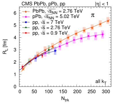
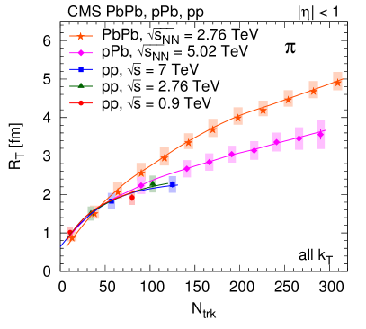
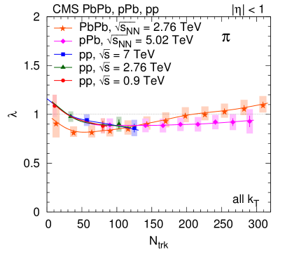
Figure 25: Track-multiplicity ($N_{\text{trk}}$) dependence of the 2D pion radius parameters $R_{\text{L}}$ and $R_{\text{T}}$ (top), and intercept parameter $\lambda$ (bottom), obtained from fits (integrated over all $\kt$) for all collision systems studied. For better visibility, only every second measurement is plotted. Lines are drawn to guide the eye.

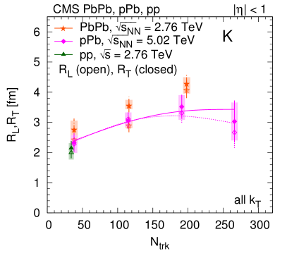
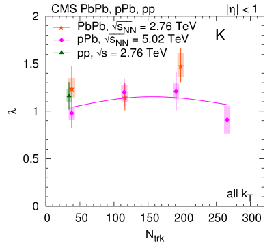
Figure 26: Track-multiplicity ($N_{\text{trk}}$) dependence of the 2D kaon radius parameters (left; $R_{\text{L}}$ – open symbols, $R_{\text{T}}$ – closed symbols) and intercept parameter $\lambda$ (right), obtained from fits (integrated over all $\kt$) for all collision systems studied. For better visibility, only every second measurement is plotted. Lines are drawn to guide the eye.

The $N_{\text{trk}}$ dependence of the 3D radii and the corresponding intercept parameters for pions (Eq. (10)), in several bins for all studied systems are shown in Fig. 27. The 3D pion radius parameters also show a similar pattern. The values of $R_{\text{L}}$, $R_{\text{O}}$, and $R_{\text{T}}$ are similar for $\Pp\Pp$ and $\Pp$Pb collisions in all bins. In general $R_{\text{L}}>R_{\text{S}}>R_{\text{O}}$, indicating once again that the source is elongated along the beam, which once more coincides with the behavior seen in $\Pp\Pp$ collisions with the double ratio technique in Section 0.5.1. In the case of PbPb collisions, $R_{\text{L}}\approx R_{\text{O}}\approx R_{\text{S}}$, indicating that the source is approximately symmetric. In addition, PbPb data show a slightly different $N_{\text{trk}}$ dependence. The $R_{\text{L}}$ radii extracted from the two- and three-dimensional fits differ slightly. While they are the same within statistical uncertainties for $\Pp\Pp$ collisions at $\sqrt{s}=0.9$, the 3D radii are on average smaller by 0.15fm for $\Pp\Pp$ collisions at $\sqrt{s}=2.76$, by 0.3fm for $\Pp\Pp$ collisions at $\sqrt{s}=7$and $\Pp$Pb collisions at $\sqrt{\smash[b]{s_{{}_{\text{NN}}}}}=5.02$, and by 0.5fm for PbPb collisions at $\sqrt{\smash[b]{s_{{}_{\text{NN}}}}}=2.76$. The most visible distinction between $\Pp\Pp$, $\Pp$Pb and PbPb data is observed in $R_{\text{O}}$, which could point to a different lifetime, $\tau$, of the created systems in those collisions, since the outward radius is related to the emitting source lifetime by $R_{\text{O}}^{2}=(R_{O}^{{}^{G}})^{2}+\tau^{2}\beta_{T}^{2}$, as discussed in Section 0.4.4.

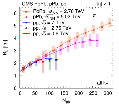
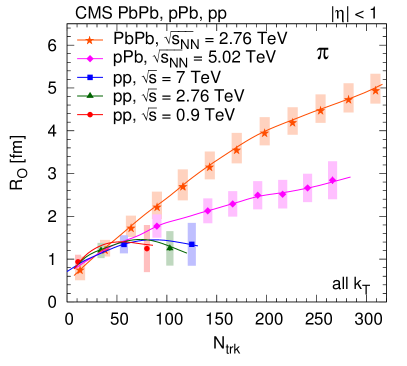
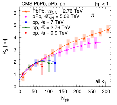
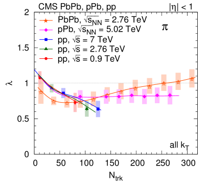
Figure 27: Track-multiplicity ($N_{\text{trk}}$) dependence of the 3D pion radius parameters $R_{\text{L}}$ (top left), $R_{\text{O}}$ (top right), $R_{\text{S}}$ (bottom left), and the intercept parameter $\lambda$ (bottom right), obtained from fits (integrated over all $\kt$) for all collision systems studied. For better visibility, only every second measurement is plotted. Lines are drawn to guide the eye.

0.6.2 Scaling for pions

The extracted radius parameters for pions are in the 1–5fm range, reaching their largest values for very high multiplicity $\Pp$Pb collisions, as well as for similar multiplicity PbPb collisions, and decrease with increasing $\kt$. By fitting the radii with a product of two independent functions of $N_{\text{trk}}$ and $\kt$, the dependencies on multiplicity and pair momentum can be factorized. For that purpose, we have used the following functional form:

$${R_{\text{param}}}(N_{\text{trk}},\kt)=\bigl{[}a^{2}+(bN_{\text{trk}}^{\beta})^{2}\bigr{]}^{1/2}\,\left(0.2\GeV/\kt\right)^{\gamma},$$ (15)

where the minimal radius $a$ and the exponent $\gamma$ of $\kt$ are kept fixed for a given radius component, for all collision types. This choice of parametrization is based on previous results [51], namely the minimal radius can be connected to the size of the proton, while the power law dependence on $N_{\text{trk}}$ is often attributed to the freeze-out density of hadrons.

We demonstrate the performance of the functional form of Eq. (15) by scaling one of the two variables ($N_{\text{trk}}$ or $\kt$) to a common value and showing the dependence on the other. Radius parameters scaled to $\kt=0.45\GeV$, that is $R(\kt/0.45\GeV)^{\gamma}$, as a function of $N_{\text{trk}}$ are shown in the left panels of Figs. 28 and  29. The ratio of the radius parameter over the value of the above parametrization at $\kt=0.45\GeV$, that is $R/R_{\text{param}}(N_{\text{trk}},\kt=0.45\GeV)$, as a function $\kt$ is shown in the right panels of Figs. 28 and  29. The obtained parameter values are listed in Table 0.6.2. The estimated uncertainty on the parameters is about 10%, based on the joint goodness-of-fits with the above functional form. Overall the proposed factorization works reasonably well.

Values of the 1D, 2D, and 3D fit parameters for pions using Eq. (15) in $\Pp\Pp$, $\Pp$Pb and PbPb collisions. The estimated uncertainty in the parameters is about 10%. cccccc@  ccc@  ccc Radius $a$ pp $\Pp$Pb PbPb $\gamma$
[fm] $b$ [fm] $\beta$ $b$ [fm] $\beta$ $b$ [fm] $\beta$
1D $R_{\text{inv}}$ 1.02 0.27 0.53 0.32 0.49 0.24 0.57 0.18
2D $R_{\text{L}}$ 1.18 0.60 0.37 0.54 0.40 0.39 0.49 0.39
$R_{\text{T}}$ 0.01 0.46 0.38 0.43 0.41 0.24 0.56 0.29
3D $R_{\text{L}}$ 1.39 0.69 0.26 0.42 0.44 0.21 0.59 0.47
$R_{\text{O}}$ 0.03 0.93 0.18 0.56 0.37 0.24 0.58 0.71
$R_{\text{S}}$ 0.03 0.47 0.34 0.33 0.44 0.18 0.58 0.20

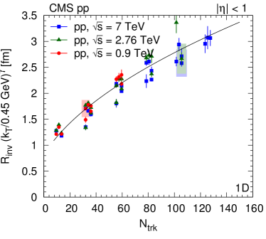
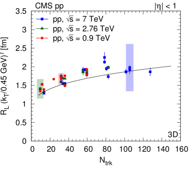
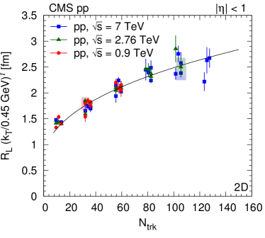
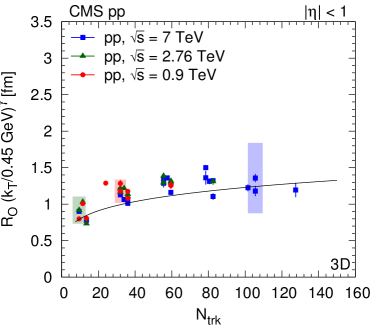
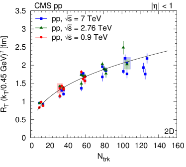
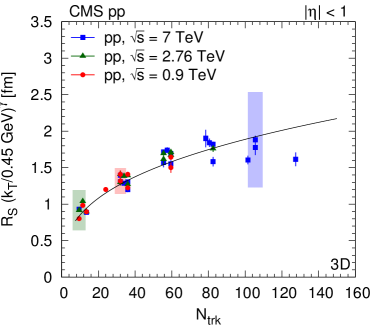
Figure 28: Radius parameters for pions as a function of $N_{\text{trk}}$ scaled to $\kt=0.45\GeV$ with help of the parametrization, as $R(\kt/0.45\GeV)^{\gamma}$ (Eq. (15)) for $\Pp\Pp$ collisions. (For better visibility, systematic uncertainties are indicated with shaded boxes, only for a fraction of the points.) Left column, from upper to lower: $R_{\text{inv}}$ from the 1D ($q_{\text{inv}}$) analysis, $R_{\text{L}}$ and $R_{\text{T}}$ from the 2D $(q_{\text{L}},q_{\text{T}})$ analysis. Right column, from upper to lower: $R_{\text{L}}$, $R_{\text{O}}$, and $R_{\text{S}}$ from the 3D $(q_{\text{L}},q_{\text{O}},q_{\text{S}})$ analysis. Fit results are indicated in the figures, see text for details.

0.7 Summary and conclusions

Detailed studies have been presented on femtoscopic correlations between pairs of same-sign hadrons produced in $\Pp\Pp$ collisions at $\sqrt{s}=0.9$, 2.76, and 7, as well as in $\Pp$Pb collisions at $\sqrt{\smash[b]{s_{{}_{\text{NN}}}}}=5.02$and peripheral PbPb collisions at $\sqrt{\smash[b]{s_{{}_{\text{NN}}}}}=2.76$. The characteristics of two-particle Bose–Einstein correlations are investigated in one ($R_{\text{inv}}$), two ($R_{\text{T}}$ and $R_{\text{L}}$), and three ($R_{\text{L}}$, $R_{\text{S}}$, and $R_{\text{O}}$) dimensions, as functions of charged multiplicity $N_{\text{trk}}$ and pair average transverse momentum $\kt$.

Two different analysis techniques are employed. The first “double ratio” technique is used to study Bose–Einstein correlations of pairs of charged hadrons emitted in $\Pp\Pp$ collisions at $\sqrt{s}=2.76$ and 7, both in the collision center-of-mass frame and in the local co-moving system. The second “particle identification and cluster subtraction” method is used to study the characteristics of two-particle correlation functions of identical charged pions and kaons, identified via their energy loss in the CMS silicon tracker, in collisions of $\Pp\Pp$, $\Pp$Pb, and peripheral PbPb collisions at various center-of-mass energies. The similarities and differences between the three colliding systems have been investigated.

The quantum correlations are well described by an exponential parametrization as a function of the relative momentum of the particle pair, both in one and in multiple dimensions, consistent with a Cauchy-Lorentz spatial source distribution. The fitted radius parameters of the emitting source, obtained for inclusive charged hadrons as well as for identified pions, increase along with charged-particle multiplicity for all colliding systems and center-of-mass energies, for one, two, and three dimensions alike. The radii are in the range 1–5fm, reaching the largest values for very high multiplicity $\Pp$Pb collisions, close to those observed in peripheral PbPb collisions with similar multiplicity. In the one-dimensional case, $R_{\text{inv}}$ in $\Pp\Pp$ collisions steadily increases with the charged multiplicity following a $N_{\text{trk}}^{1/3}$ dependence, as well as showing an approximate independence of the center-of-mass energy. This behavior is also observed for the longitudinal radius parameter ($R_{\text{L}}^{*}$ in the center-of-mass frame, and $R_{\text{L}}$ in the local co-moving system) in the two-dimensional case.

The multiplicity dependence of $R_{\text{L}}$ and $R_{\text{T}}$ is similar for $\Pp\Pp$ and $\Pp$Pb collisions in all $\kt$ bins, and that similarity also applies to peripheral PbPb collisions for $\kt>$ 0.4. In general, the observed orderings, $R_{\text{L}}>R_{\text{T}}$ and $R_{\text{L}}\gtrsim R_{\text{S}}>R_{\text{O}}$, indicate that the $\Pp\Pp$ and $\Pp$Pb sources are elongated in the beam direction. For peripheral PbPb collisions, the source is quite symmetric, and shows a slightly different $N_{\text{trk}}$ dependence, with the largest differences between the systems for $R_{\text{T}}$ and $R_{\text{O}}$, while $R_{\text{L}}$ and $R_{\text{S}}$ are approximately equal. The most visible differences between pp, $\Pp$Pb, and PbPb collisions are seen in $R_{\text{O}}$, which could point to a different lifetime of the emitting systems in the three cases. The kaon radius parameters show a smaller increase with $N_{\text{trk}}$ than observed for pions. The radius parameters of charged hadrons and pions decrease with increasing $\kt$, an observation compatible with expanding emitting sources. The $\kt$- and $N_{\text{trk}}$-dependences of the radius parameters factorize, and are largely independent of beam energy and colliding system for lower multiplicities, although some system dependence appears at higher values of $N_{\text{trk}}$.

A shallow anticorrelation (a region where the correlation function falls below one) observed using the double ratio technique in a previous analysis of $\Pp\Pp$ collisions, is also seen in the present data. The depth of this dip in the one-dimensional correlation functions decreases with increasing particle multiplicity and also decreases slightly with increasing $\kt$.

Finally, the similar multiplicity dependencies of the radii extracted for $\Pp\Pp$, $\Pp$Pb, and peripheral PbPb collisions suggest a common freeze-out density of hadrons for all collision systems, since the correlation techniques measure the characteristic size of the system near the time of the last interactions. In the case of $\Pp\Pp$ collisions, extending the investigation of these similarities to higher multiplicities than those accessible with the current data can provide new information on final state collective effects in such events.

.8 The CMS Collaboration

Yerevan Physics Institute, Yerevan, Armenia
A.M. Sirunyan, A. Tumasyan Institut für Hochenergiephysik, Wien, Austria
W. Adam, F. Ambrogi, E. Asilar, T. Bergauer, J. Brandstetter, E. Brondolin, M. Dragicevic, J. Erö, M. Flechl, M. Friedl, R. Frühwirth1, V.M. Ghete, J. Grossmann, J. Hrubec, M. Jeitler1, A. König, N. Krammer, I. Krätschmer, D. Liko, T. Madlener, I. Mikulec, E. Pree, D. Rabady, N. Rad, H. Rohringer, J. Schieck1, R. Schöfbeck, M. Spanring, D. Spitzbart, J. Strauss, W. Waltenberger, J. Wittmann, C.-E. Wulz1, M. Zarucki Institute for Nuclear Problems, Minsk, Belarus
V. Chekhovsky, V. Mossolov, J. Suarez Gonzalez Universiteit Antwerpen, Antwerpen, Belgium
E.A. De Wolf, D. Di Croce, X. Janssen, J. Lauwers, M. Van De Klundert, H. Van Haevermaet, P. Van Mechelen, N. Van Remortel Vrije Universiteit Brussel, Brussel, Belgium
S. Abu Zeid, F. Blekman, J. D’Hondt, I. De Bruyn, J. De Clercq, K. Deroover, G. Flouris, D. Lontkovskyi, S. Lowette, S. Moortgat, L. Moreels, A. Olbrechts, Q. Python, K. Skovpen, S. Tavernier, W. Van Doninck, P. Van Mulders, I. Van Parijs Université Libre de Bruxelles, Bruxelles, Belgium
H. Brun, B. Clerbaux, G. De Lentdecker, H. Delannoy, G. Fasanella, L. Favart, R. Goldouzian, A. Grebenyuk, G. Karapostoli, T. Lenzi, J. Luetic, T. Maerschalk, A. Marinov, A. Randle-conde, T. Seva, C. Vander Velde, P. Vanlaer, D. Vannerom, R. Yonamine, F. Zenoni, F. Zhang2 Ghent University, Ghent, Belgium
A. Cimmino, T. Cornelis, D. Dobur, A. Fagot, M. Gul, I. Khvastunov, D. Poyraz, C. Roskas, S. Salva, M. Tytgat, W. Verbeke, N. Zaganidis Université Catholique de Louvain, Louvain-la-Neuve, Belgium
H. Bakhshiansohi, O. Bondu, S. Brochet, G. Bruno, A. Caudron, S. De Visscher, C. Delaere, M. Delcourt, B. Francois, A. Giammanco, A. Jafari, M. Komm, G. Krintiras, V. Lemaitre, A. Magitteri, A. Mertens, M. Musich, K. Piotrzkowski, L. Quertenmont, M. Vidal Marono, S. Wertz Université de Mons, Mons, Belgium
N. Beliy Centro Brasileiro de Pesquisas Fisicas, Rio de Janeiro, Brazil
W.L. Aldá Júnior, F.L. Alves, G.A. Alves, L. Brito, M. Correa Martins Junior, C. Hensel, A. Moraes, M.E. Pol, P. Rebello Teles Universidade do Estado do Rio de Janeiro, Rio de Janeiro, Brazil
E. Belchior Batista Das Chagas, W. Carvalho, J. Chinellato3, A. Custódio, E.M. Da Costa, G.G. Da Silveira4, D. De Jesus Damiao, S. Fonseca De Souza, L.M. Huertas Guativa, H. Malbouisson, M. Melo De Almeida, C. Mora Herrera, L. Mundim, H. Nogima, A. Santoro, A. Sznajder, E.J. Tonelli Manganote3, F. Torres Da Silva De Araujo, A. Vilela Pereira Universidade Estadual Paulista ${}^{a}$, Universidade Federal do ABC ${}^{b}$, São Paulo, Brazil
S. Ahuja${}^{a}$, C.A. Bernardes${}^{a}$, S. Dogra${}^{a}$, T.R. Fernandez Perez Tomei${}^{a}$, E.M. Gregores${}^{b}$, P.G. Mercadante${}^{b}$, S.F. Novaes${}^{a}$, Sandra S. Padula${}^{a}$, D. Romero Abad${}^{b}$, J.C. Ruiz Vargas${}^{a}$ Institute for Nuclear Research and Nuclear Energy, Bulgarian Academy of Sciences, Sofia, Bulgaria
A. Aleksandrov, R. Hadjiiska, P. Iaydjiev, M. Misheva, M. Rodozov, M. Shopova, S. Stoykova, G. Sultanov University of Sofia, Sofia, Bulgaria
A. Dimitrov, I. Glushkov, L. Litov, B. Pavlov, P. Petkov Beihang University, Beijing, China
W. Fang5, X. Gao5 Institute of High Energy Physics, Beijing, China
M. Ahmad, J.G. Bian, G.M. Chen, H.S. Chen, M. Chen, Y. Chen, C.H. Jiang, D. Leggat, H. Liao, Z. Liu, F. Romeo, S.M. Shaheen, A. Spiezia, J. Tao, C. Wang, Z. Wang, E. Yazgan, H. Zhang, J. Zhao State Key Laboratory of Nuclear Physics and Technology, Peking University, Beijing, China
Y. Ban, G. Chen, Q. Li, S. Liu, Y. Mao, S.J. Qian, D. Wang, Z. Xu Universidad de Los Andes, Bogota, Colombia
C. Avila, A. Cabrera, C.A. Carrillo Montoya, L.F. Chaparro Sierra, C. Florez, C.F. González Hernández, J.D. Ruiz Alvarez University of Split, Faculty of Electrical Engineering, Mechanical Engineering and Naval Architecture, Split, Croatia
B. Courbon, N. Godinovic, D. Lelas, I. Puljak, P.M. Ribeiro Cipriano, T. Sculac University of Split, Faculty of Science, Split, Croatia
Z. Antunovic, M. Kovac Institute Rudjer Boskovic, Zagreb, Croatia
V. Brigljevic, D. Ferencek, K. Kadija, B. Mesic, A. Starodumov6, T. Susa University of Cyprus, Nicosia, Cyprus
M.W. Ather, A. Attikis, G. Mavromanolakis, J. Mousa, C. Nicolaou, F. Ptochos, P.A. Razis, H. Rykaczewski Charles University, Prague, Czech Republic
M. Finger7, M. Finger Jr.7 Universidad San Francisco de Quito, Quito, Ecuador
E. Carrera Jarrin Academy of Scientific Research and Technology of the Arab Republic of Egypt, Egyptian Network of High Energy Physics, Cairo, Egypt
Y. Assran8${}^{,}$9, M.A. Mahmoud10${}^{,}$9, A. Mahrous11 National Institute of Chemical Physics and Biophysics, Tallinn, Estonia
R.K. Dewanjee, M. Kadastik, L. Perrini, M. Raidal, A. Tiko, C. Veelken Department of Physics, University of Helsinki, Helsinki, Finland
P. Eerola, J. Pekkanen, M. Voutilainen Helsinki Institute of Physics, Helsinki, Finland
J. Härkönen, T. Järvinen, V. Karimäki, R. Kinnunen, T. Lampén, K. Lassila-Perini, S. Lehti, T. Lindén, P. Luukka, E. Tuominen, J. Tuominiemi, E. Tuovinen Lappeenranta University of Technology, Lappeenranta, Finland
J. Talvitie, T. Tuuva IRFU, CEA, Université Paris-Saclay, Gif-sur-Yvette, France
M. Besancon, F. Couderc, M. Dejardin, D. Denegri, J.L. Faure, F. Ferri, S. Ganjour, S. Ghosh, A. Givernaud, P. Gras, G. Hamel de Monchenault, P. Jarry, I. Kucher, E. Locci, M. Machet, J. Malcles, G. Negro, J. Rander, A. Rosowsky, M.Ö. Sahin, M. Titov Laboratoire Leprince-Ringuet, Ecole polytechnique, CNRS/IN2P3, Université Paris-Saclay, Palaiseau, France
A. Abdulsalam, I. Antropov, S. Baffioni, F. Beaudette, P. Busson, L. Cadamuro, C. Charlot, R. Granier de Cassagnac, M. Jo, S. Lisniak, A. Lobanov, J. Martin Blanco, M. Nguyen, C. Ochando, G. Ortona, P. Paganini, P. Pigard, S. Regnard, R. Salerno, J.B. Sauvan, Y. Sirois, A.G. Stahl Leiton, T. Strebler, Y. Yilmaz, A. Zabi, A. Zghiche Université de Strasbourg, CNRS, IPHC UMR 7178, F-67000 Strasbourg, France
J.-L. Agram12, J. Andrea, D. Bloch, J.-M. Brom, M. Buttignol, E.C. Chabert, N. Chanon, C. Collard, E. Conte12, X. Coubez, J.-C. Fontaine12, D. Gelé, U. Goerlach, M. Jansová, A.-C. Le Bihan, N. Tonon, P. Van Hove Centre de Calcul de l’Institut National de Physique Nucleaire et de Physique des Particules, CNRS/IN2P3, Villeurbanne, France
S. Gadrat Université de Lyon, Université Claude Bernard Lyon 1, CNRS-IN2P3, Institut de Physique Nucléaire de Lyon, Villeurbanne, France
S. Beauceron, C. Bernet, G. Boudoul, R. Chierici, D. Contardo, P. Depasse, H. El Mamouni, J. Fay, L. Finco, S. Gascon, M. Gouzevitch, G. Grenier, B. Ille, F. Lagarde, I.B. Laktineh, M. Lethuillier, L. Mirabito, A.L. Pequegnot, S. Perries, A. Popov13, V. Sordini, M. Vander Donckt, S. Viret Georgian Technical University, Tbilisi, Georgia
T. Toriashvili14 Tbilisi State University, Tbilisi, Georgia
Z. Tsamalaidze7 RWTH Aachen University, I. Physikalisches Institut, Aachen, Germany
C. Autermann, S. Beranek, L. Feld, M.K. Kiesel, K. Klein, M. Lipinski, M. Preuten, C. Schomakers, J. Schulz, T. Verlage RWTH Aachen University, III. Physikalisches Institut A, Aachen, Germany
A. Albert, E. Dietz-Laursonn, D. Duchardt, M. Endres, M. Erdmann, S. Erdweg, T. Esch, R. Fischer, A. Güth, M. Hamer, T. Hebbeker, C. Heidemann, K. Hoepfner, S. Knutzen, M. Merschmeyer, A. Meyer, P. Millet, S. Mukherjee, M. Olschewski, K. Padeken, T. Pook, M. Radziej, H. Reithler, M. Rieger, F. Scheuch, D. Teyssier, S. Thüer RWTH Aachen University, III. Physikalisches Institut B, Aachen, Germany
G. Flügge, B. Kargoll, T. Kress, A. Künsken, J. Lingemann, T. Müller, A. Nehrkorn, A. Nowack, C. Pistone, O. Pooth, A. Stahl15 Deutsches Elektronen-Synchrotron, Hamburg, Germany
M. Aldaya Martin, T. Arndt, C. Asawatangtrakuldee, K. Beernaert, O. Behnke, U. Behrens, A. Bermúdez Martínez, A.A. Bin Anuar, K. Borras16, V. Botta, A. Campbell, P. Connor, C. Contreras-Campana, F. Costanza, C. Diez Pardos, G. Eckerlin, D. Eckstein, T. Eichhorn, E. Eren, E. Gallo17, J. Garay Garcia, A. Geiser, A. Gizhko, J.M. Grados Luyando, A. Grohsjean, P. Gunnellini, A. Harb, J. Hauk, M. Hempel18, H. Jung, A. Kalogeropoulos, M. Kasemann, J. Keaveney, C. Kleinwort, I. Korol, D. Krücker, W. Lange, A. Lelek, T. Lenz, J. Leonard, K. Lipka, W. Lohmann18, R. Mankel, I.-A. Melzer-Pellmann, A.B. Meyer, G. Mittag, J. Mnich, A. Mussgiller, E. Ntomari, D. Pitzl, R. Placakyte, A. Raspereza, B. Roland, M. Savitskyi, P. Saxena, R. Shevchenko, S. Spannagel, N. Stefaniuk, G.P. Van Onsem, R. Walsh, Y. Wen, K. Wichmann, C. Wissing, O. Zenaiev University of Hamburg, Hamburg, Germany
S. Bein, V. Blobel, M. Centis Vignali, T. Dreyer, E. Garutti, D. Gonzalez, J. Haller, A. Hinzmann, M. Hoffmann, A. Karavdina, R. Klanner, R. Kogler, N. Kovalchuk, S. Kurz, T. Lapsien, I. Marchesini, D. Marconi, M. Meyer, M. Niedziela, D. Nowatschin, F. Pantaleo15, T. Peiffer, A. Perieanu, C. Scharf, P. Schleper, A. Schmidt, S. Schumann, J. Schwandt, J. Sonneveld, H. Stadie, G. Steinbrück, F.M. Stober, M. Stöver, H. Tholen, D. Troendle, E. Usai, L. Vanelderen, A. Vanhoefer, B. Vormwald Institut für Experimentelle Kernphysik, Karlsruhe, Germany
M. Akbiyik, C. Barth, S. Baur, E. Butz, R. Caspart, T. Chwalek, F. Colombo, W. De Boer, A. Dierlamm, B. Freund, R. Friese, M. Giffels, A. Gilbert, D. Haitz, F. Hartmann15, S.M. Heindl, U. Husemann, F. Kassel15, S. Kudella, H. Mildner, M.U. Mozer, Th. Müller, M. Plagge, G. Quast, K. Rabbertz, M. Schröder, I. Shvetsov, G. Sieber, H.J. Simonis, R. Ulrich, S. Wayand, M. Weber, T. Weiler, S. Williamson, C. Wöhrmann, R. Wolf Institute of Nuclear and Particle Physics (INPP), NCSR Demokritos, Aghia Paraskevi, Greece
G. Anagnostou, G. Daskalakis, T. Geralis, V.A. Giakoumopoulou, A. Kyriakis, D. Loukas, I. Topsis-Giotis National and Kapodistrian University of Athens, Athens, Greece
S. Kesisoglou, A. Panagiotou, N. Saoulidou University of Ioánnina, Ioánnina, Greece
I. Evangelou, C. Foudas, P. Kokkas, S. Mallios, N. Manthos, I. Papadopoulos, E. Paradas, J. Strologas, F.A. Triantis MTA-ELTE Lendület CMS Particle and Nuclear Physics Group, Eötvös Loránd University, Budapest, Hungary
M. Csanad, N. Filipovic, G. Pasztor Wigner Research Centre for Physics, Budapest, Hungary
G. Bencze, C. Hajdu, D. Horvath19, Á. Hunyadi, F. Sikler, V. Veszpremi, G. Vesztergombi20, A.J. Zsigmond Institute of Nuclear Research ATOMKI, Debrecen, Hungary
N. Beni, S. Czellar, J. Karancsi21, A. Makovec, J. Molnar, Z. Szillasi Institute of Physics, University of Debrecen, Debrecen, Hungary
M. Bartók20, P. Raics, Z.L. Trocsanyi, B. Ujvari Indian Institute of Science (IISc), Bangalore, India
S. Choudhury, J.R. Komaragiri National Institute of Science Education and Research, Bhubaneswar, India
S. Bahinipati22, S. Bhowmik, P. Mal, K. Mandal, A. Nayak23, D.K. Sahoo22, N. Sahoo, S.K. Swain Panjab University, Chandigarh, India
S. Bansal, S.B. Beri, V. Bhatnagar, U. Bhawandeep, R. Chawla, N. Dhingra, A.K. Kalsi, A. Kaur, M. Kaur, R. Kumar, P. Kumari, A. Mehta, J.B. Singh, G. Walia University of Delhi, Delhi, India
A. Bhardwaj, S. Chauhan, B.C. Choudhary, R.B. Garg, S. Keshri, A. Kumar, Ashok Kumar, S. Malhotra, M. Naimuddin, K. Ranjan, Aashaq Shah, R. Sharma, V. Sharma Saha Institute of Nuclear Physics, HBNI, Kolkata, India
R. Bhardwaj, R. Bhattacharya, S. Bhattacharya, S. Dey, S. Dutt, S. Dutta, S. Ghosh, N. Majumdar, A. Modak, K. Mondal, S. Mukhopadhyay, S. Nandan, A. Purohit, A. Roy, D. Roy, S. Roy Chowdhury, S. Sarkar, M. Sharan, S. Thakur Indian Institute of Technology Madras, Madras, India
P.K. Behera Bhabha Atomic Research Centre, Mumbai, India
R. Chudasama, D. Dutta, V. Jha, V. Kumar, A.K. Mohanty15, P.K. Netrakanti, L.M. Pant, P. Shukla, A. Topkar Tata Institute of Fundamental Research-A, Mumbai, India
T. Aziz, S. Dugad, B. Mahakud, S. Mitra, G.B. Mohanty, N. Sur, B. Sutar Tata Institute of Fundamental Research-B, Mumbai, India
S. Banerjee, S. Bhattacharya, S. Chatterjee, P. Das, M. Guchait, Sa. Jain, S. Kumar, M. Maity24, G. Majumder, K. Mazumdar, T. Sarkar24, N. Wickramage25 Indian Institute of Science Education and Research (IISER), Pune, India
S. Chauhan, S. Dube, V. Hegde, A. Kapoor, K. Kothekar, S. Pandey, A. Rane, S. Sharma Institute for Research in Fundamental Sciences (IPM), Tehran, Iran
S. Chenarani26, E. Eskandari Tadavani, S.M. Etesami26, M. Khakzad, M. Mohammadi Najafabadi, M. Naseri, S. Paktinat Mehdiabadi27, F. Rezaei Hosseinabadi, B. Safarzadeh28, M. Zeinali University College Dublin, Dublin, Ireland
M. Felcini, M. Grunewald INFN Sezione di Bari ${}^{a}$, Università di Bari ${}^{b}$, Politecnico di Bari ${}^{c}$, Bari, Italy
M. Abbrescia${}^{a}$${}^{,}$${}^{b}$, C. Calabria${}^{a}$${}^{,}$${}^{b}$, C. Caputo${}^{a}$${}^{,}$${}^{b}$, A. Colaleo${}^{a}$, D. Creanza${}^{a}$${}^{,}$${}^{c}$, L. Cristella${}^{a}$${}^{,}$${}^{b}$, N. De Filippis${}^{a}$${}^{,}$${}^{c}$, M. De Palma${}^{a}$${}^{,}$${}^{b}$, F. Errico${}^{a}$${}^{,}$${}^{b}$, L. Fiore${}^{a}$, G. Iaselli${}^{a}$${}^{,}$${}^{c}$, S. Lezki${}^{a}$${}^{,}$${}^{b}$, G. Maggi${}^{a}$${}^{,}$${}^{c}$, M. Maggi${}^{a}$, G. Miniello${}^{a}$${}^{,}$${}^{b}$, S. My${}^{a}$${}^{,}$${}^{b}$, S. Nuzzo${}^{a}$${}^{,}$${}^{b}$, A. Pompili${}^{a}$${}^{,}$${}^{b}$, G. Pugliese${}^{a}$${}^{,}$${}^{c}$, R. Radogna${}^{a}$${}^{,}$${}^{b}$, A. Ranieri${}^{a}$, G. Selvaggi${}^{a}$${}^{,}$${}^{b}$, A. Sharma${}^{a}$, L. Silvestris${}^{a}$${}^{,}$15, R. Venditti${}^{a}$, P. Verwilligen${}^{a}$ INFN Sezione di Bologna ${}^{a}$, Università di Bologna ${}^{b}$, Bologna, Italy
G. Abbiendi${}^{a}$, C. Battilana${}^{a}$${}^{,}$${}^{b}$, D. Bonacorsi${}^{a}$${}^{,}$${}^{b}$, S. Braibant-Giacomelli${}^{a}$${}^{,}$${}^{b}$, R. Campanini${}^{a}$${}^{,}$${}^{b}$, P. Capiluppi${}^{a}$${}^{,}$${}^{b}$, A. Castro${}^{a}$${}^{,}$${}^{b}$, F.R. Cavallo${}^{a}$, S.S. Chhibra${}^{a}$, G. Codispoti${}^{a}$${}^{,}$${}^{b}$, M. Cuffiani${}^{a}$${}^{,}$${}^{b}$, G.M. Dallavalle${}^{a}$, F. Fabbri${}^{a}$, A. Fanfani${}^{a}$${}^{,}$${}^{b}$, D. Fasanella${}^{a}$${}^{,}$${}^{b}$, P. Giacomelli${}^{a}$, C. Grandi${}^{a}$, L. Guiducci${}^{a}$${}^{,}$${}^{b}$, S. Marcellini${}^{a}$, G. Masetti${}^{a}$, A. Montanari${}^{a}$, F.L. Navarria${}^{a}$${}^{,}$${}^{b}$, A. Perrotta${}^{a}$, A.M. Rossi${}^{a}$${}^{,}$${}^{b}$, T. Rovelli${}^{a}$${}^{,}$${}^{b}$, G.P. Siroli${}^{a}$${}^{,}$${}^{b}$, N. Tosi${}^{a}$ INFN Sezione di Catania ${}^{a}$, Università di Catania ${}^{b}$, Catania, Italy
S. Albergo${}^{a}$${}^{,}$${}^{b}$, S. Costa${}^{a}$${}^{,}$${}^{b}$, A. Di Mattia${}^{a}$, F. Giordano${}^{a}$${}^{,}$${}^{b}$, R. Potenza${}^{a}$${}^{,}$${}^{b}$, A. Tricomi${}^{a}$${}^{,}$${}^{b}$, C. Tuve${}^{a}$${}^{,}$${}^{b}$ INFN Sezione di Firenze ${}^{a}$, Università di Firenze ${}^{b}$, Firenze, Italy
G. Barbagli${}^{a}$, K. Chatterjee${}^{a}$${}^{,}$${}^{b}$, V. Ciulli${}^{a}$${}^{,}$${}^{b}$, C. Civinini${}^{a}$, R. D’Alessandro${}^{a}$${}^{,}$${}^{b}$, E. Focardi${}^{a}$${}^{,}$${}^{b}$, P. Lenzi${}^{a}$${}^{,}$${}^{b}$, M. Meschini${}^{a}$, S. Paoletti${}^{a}$, L. Russo${}^{a}$${}^{,}$29, G. Sguazzoni${}^{a}$, D. Strom${}^{a}$, L. Viliani${}^{a}$${}^{,}$${}^{b}$${}^{,}$15 INFN Laboratori Nazionali di Frascati, Frascati, Italy
L. Benussi, S. Bianco, F. Fabbri, D. Piccolo, F. Primavera15 INFN Sezione di Genova ${}^{a}$, Università di Genova ${}^{b}$, Genova, Italy
V. Calvelli${}^{a}$${}^{,}$${}^{b}$, F. Ferro${}^{a}$, E. Robutti${}^{a}$, S. Tosi${}^{a}$${}^{,}$${}^{b}$ INFN Sezione di Milano-Bicocca ${}^{a}$, Università di Milano-Bicocca ${}^{b}$, Milano, Italy
L. Brianza${}^{a}$${}^{,}$${}^{b}$, F. Brivio${}^{a}$${}^{,}$${}^{b}$, V. Ciriolo${}^{a}$${}^{,}$${}^{b}$, M.E. Dinardo${}^{a}$${}^{,}$${}^{b}$, S. Fiorendi${}^{a}$${}^{,}$${}^{b}$, S. Gennai${}^{a}$, A. Ghezzi${}^{a}$${}^{,}$${}^{b}$, P. Govoni${}^{a}$${}^{,}$${}^{b}$, M. Malberti${}^{a}$${}^{,}$${}^{b}$, S. Malvezzi${}^{a}$, R.A. Manzoni${}^{a}$${}^{,}$${}^{b}$, D. Menasce${}^{a}$, L. Moroni${}^{a}$, M. Paganoni${}^{a}$${}^{,}$${}^{b}$, K. Pauwels${}^{a}$${}^{,}$${}^{b}$, D. Pedrini${}^{a}$, S. Pigazzini${}^{a}$${}^{,}$${}^{b}$${}^{,}$30, S. Ragazzi${}^{a}$${}^{,}$${}^{b}$, T. Tabarelli de Fatis${}^{a}$${}^{,}$${}^{b}$ INFN Sezione di Napoli ${}^{a}$, Università di Napoli ’Federico II’ ${}^{b}$, Napoli, Italy, Università della Basilicata ${}^{c}$, Potenza, Italy, Università G. Marconi ${}^{d}$, Roma, Italy
S. Buontempo${}^{a}$, N. Cavallo${}^{a}$${}^{,}$${}^{c}$, S. Di Guida${}^{a}$${}^{,}$${}^{d}$${}^{,}$15, F. Fabozzi${}^{a}$${}^{,}$${}^{c}$, F. Fienga${}^{a}$${}^{,}$${}^{b}$, A.O.M. Iorio${}^{a}$${}^{,}$${}^{b}$, W.A. Khan${}^{a}$, L. Lista${}^{a}$, S. Meola${}^{a}$${}^{,}$${}^{d}$${}^{,}$15, P. Paolucci${}^{a}$${}^{,}$15, C. Sciacca${}^{a}$${}^{,}$${}^{b}$, F. Thyssen${}^{a}$ INFN Sezione di Padova ${}^{a}$, Università di Padova ${}^{b}$, Padova, Italy, Università di Trento ${}^{c}$, Trento, Italy
P. Azzi${}^{a}$${}^{,}$15, N. Bacchetta${}^{a}$, L. Benato${}^{a}$${}^{,}$${}^{b}$, D. Bisello${}^{a}$${}^{,}$${}^{b}$, A. Boletti${}^{a}$${}^{,}$${}^{b}$, R. Carlin${}^{a}$${}^{,}$${}^{b}$, A. Carvalho Antunes De Oliveira${}^{a}$${}^{,}$${}^{b}$, P. Checchia${}^{a}$, P. De Castro Manzano${}^{a}$, T. Dorigo${}^{a}$, U. Dosselli${}^{a}$, F. Gasparini${}^{a}$${}^{,}$${}^{b}$, U. Gasparini${}^{a}$${}^{,}$${}^{b}$, F. Gonella${}^{a}$, A. Gozzelino${}^{a}$, M. Gulmini${}^{a}$${}^{,}$31, S. Lacaprara${}^{a}$, P. Lujan, M. Margoni${}^{a}$${}^{,}$${}^{b}$, N. Pozzobon${}^{a}$${}^{,}$${}^{b}$, P. Ronchese${}^{a}$${}^{,}$${}^{b}$, R. Rossin${}^{a}$${}^{,}$${}^{b}$, M. Zanetti${}^{a}$${}^{,}$${}^{b}$, P. Zotto${}^{a}$${}^{,}$${}^{b}$, G. Zumerle${}^{a}$${}^{,}$${}^{b}$ INFN Sezione di Pavia ${}^{a}$, Università di Pavia ${}^{b}$, Pavia, Italy
A. Braghieri${}^{a}$, F. Fallavollita${}^{a}$${}^{,}$${}^{b}$, A. Magnani${}^{a}$${}^{,}$${}^{b}$, P. Montagna${}^{a}$${}^{,}$${}^{b}$, S.P. Ratti${}^{a}$${}^{,}$${}^{b}$, V. Re${}^{a}$, M. Ressegotti, C. Riccardi${}^{a}$${}^{,}$${}^{b}$, P. Salvini${}^{a}$, I. Vai${}^{a}$${}^{,}$${}^{b}$, P. Vitulo${}^{a}$${}^{,}$${}^{b}$ INFN Sezione di Perugia ${}^{a}$, Università di Perugia ${}^{b}$, Perugia, Italy
L. Alunni Solestizi${}^{a}$${}^{,}$${}^{b}$, M. Biasini${}^{a}$${}^{,}$${}^{b}$, G.M. Bilei${}^{a}$, C. Cecchi${}^{a}$${}^{,}$${}^{b}$, D. Ciangottini${}^{a}$${}^{,}$${}^{b}$, L. Fanò${}^{a}$${}^{,}$${}^{b}$, P. Lariccia${}^{a}$${}^{,}$${}^{b}$, R. Leonardi${}^{a}$${}^{,}$${}^{b}$, E. Manoni${}^{a}$, G. Mantovani${}^{a}$${}^{,}$${}^{b}$, V. Mariani${}^{a}$${}^{,}$${}^{b}$, M. Menichelli${}^{a}$, A. Rossi${}^{a}$${}^{,}$${}^{b}$, A. Santocchia${}^{a}$${}^{,}$${}^{b}$, D. Spiga${}^{a}$ INFN Sezione di Pisa ${}^{a}$, Università di Pisa ${}^{b}$, Scuola Normale Superiore di Pisa ${}^{c}$, Pisa, Italy
K. Androsov${}^{a}$, P. Azzurri${}^{a}$${}^{,}$15, G. Bagliesi${}^{a}$, J. Bernardini${}^{a}$, T. Boccali${}^{a}$, L. Borrello, R. Castaldi${}^{a}$, M.A. Ciocci${}^{a}$${}^{,}$${}^{b}$, R. Dell’Orso${}^{a}$, G. Fedi${}^{a}$, L. Giannini${}^{a}$${}^{,}$${}^{c}$, A. Giassi${}^{a}$, M.T. Grippo${}^{a}$${}^{,}$29, F. Ligabue${}^{a}$${}^{,}$${}^{c}$, T. Lomtadze${}^{a}$, E. Manca${}^{a}$${}^{,}$${}^{c}$, G. Mandorli${}^{a}$${}^{,}$${}^{c}$, L. Martini${}^{a}$${}^{,}$${}^{b}$, A. Messineo${}^{a}$${}^{,}$${}^{b}$, F. Palla${}^{a}$, A. Rizzi${}^{a}$${}^{,}$${}^{b}$, A. Savoy-Navarro${}^{a}$${}^{,}$32, P. Spagnolo${}^{a}$, R. Tenchini${}^{a}$, G. Tonelli${}^{a}$${}^{,}$${}^{b}$, A. Venturi${}^{a}$, P.G. Verdini${}^{a}$ INFN Sezione di Roma ${}^{a}$, Sapienza Università di Roma ${}^{b}$, Rome, Italy
L. Barone${}^{a}$${}^{,}$${}^{b}$, F. Cavallari${}^{a}$, M. Cipriani${}^{a}$${}^{,}$${}^{b}$, N. Daci${}^{a}$, D. Del Re${}^{a}$${}^{,}$${}^{b}$${}^{,}$15, M. Diemoz${}^{a}$, S. Gelli${}^{a}$${}^{,}$${}^{b}$, E. Longo${}^{a}$${}^{,}$${}^{b}$, F. Margaroli${}^{a}$${}^{,}$${}^{b}$, B. Marzocchi${}^{a}$${}^{,}$${}^{b}$, P. Meridiani${}^{a}$, G. Organtini${}^{a}$${}^{,}$${}^{b}$, R. Paramatti${}^{a}$${}^{,}$${}^{b}$, F. Preiato${}^{a}$${}^{,}$${}^{b}$, S. Rahatlou${}^{a}$${}^{,}$${}^{b}$, C. Rovelli${}^{a}$, F. Santanastasio${}^{a}$${}^{,}$${}^{b}$ INFN Sezione di Torino ${}^{a}$, Università di Torino ${}^{b}$, Torino, Italy, Università del Piemonte Orientale ${}^{c}$, Novara, Italy
N. Amapane${}^{a}$${}^{,}$${}^{b}$, R. Arcidiacono${}^{a}$${}^{,}$${}^{c}$, S. Argiro${}^{a}$${}^{,}$${}^{b}$, M. Arneodo${}^{a}$${}^{,}$${}^{c}$, N. Bartosik${}^{a}$, R. Bellan${}^{a}$${}^{,}$${}^{b}$, C. Biino${}^{a}$, N. Cartiglia${}^{a}$, F. Cenna${}^{a}$${}^{,}$${}^{b}$, M. Costa${}^{a}$${}^{,}$${}^{b}$, R. Covarelli${}^{a}$${}^{,}$${}^{b}$, A. Degano${}^{a}$${}^{,}$${}^{b}$, N. Demaria${}^{a}$, B. Kiani${}^{a}$${}^{,}$${}^{b}$, C. Mariotti${}^{a}$, S. Maselli${}^{a}$, E. Migliore${}^{a}$${}^{,}$${}^{b}$, V. Monaco${}^{a}$${}^{,}$${}^{b}$, E. Monteil${}^{a}$${}^{,}$${}^{b}$, M. Monteno${}^{a}$, M.M. Obertino${}^{a}$${}^{,}$${}^{b}$, L. Pacher${}^{a}$${}^{,}$${}^{b}$, N. Pastrone${}^{a}$, M. Pelliccioni${}^{a}$, G.L. Pinna Angioni${}^{a}$${}^{,}$${}^{b}$, F. Ravera${}^{a}$${}^{,}$${}^{b}$, A. Romero${}^{a}$${}^{,}$${}^{b}$, M. Ruspa${}^{a}$${}^{,}$${}^{c}$, R. Sacchi${}^{a}$${}^{,}$${}^{b}$, K. Shchelina${}^{a}$${}^{,}$${}^{b}$, V. Sola${}^{a}$, A. Solano${}^{a}$${}^{,}$${}^{b}$, A. Staiano${}^{a}$, P. Traczyk${}^{a}$${}^{,}$${}^{b}$ INFN Sezione di Trieste ${}^{a}$, Università di Trieste ${}^{b}$, Trieste, Italy
S. Belforte${}^{a}$, M. Casarsa${}^{a}$, F. Cossutti${}^{a}$, G. Della Ricca${}^{a}$${}^{,}$${}^{b}$, A. Zanetti${}^{a}$ Kyungpook National University, Daegu, Korea
D.H. Kim, G.N. Kim, M.S. Kim, J. Lee, S. Lee, S.W. Lee, C.S. Moon, Y.D. Oh, S. Sekmen, D.C. Son, Y.C. Yang Chonbuk National University, Jeonju, Korea
A. Lee Chonnam National University, Institute for Universe and Elementary Particles, Kwangju, Korea
H. Kim, D.H. Moon, G. Oh Hanyang University, Seoul, Korea
J.A. Brochero Cifuentes, J. Goh, T.J. Kim Korea University, Seoul, Korea
S. Cho, S. Choi, Y. Go, D. Gyun, S. Ha, B. Hong, Y. Jo, Y. Kim, K. Lee, K.S. Lee, S. Lee, J. Lim, S.K. Park, Y. Roh Seoul National University, Seoul, Korea
J. Almond, J. Kim, J.S. Kim, H. Lee, K. Lee, K. Nam, S.B. Oh, B.C. Radburn-Smith, S.h. Seo, U.K. Yang, H.D. Yoo, G.B. Yu University of Seoul, Seoul, Korea
M. Choi, H. Kim, J.H. Kim, J.S.H. Lee, I.C. Park, G. Ryu Sungkyunkwan University, Suwon, Korea
Y. Choi, C. Hwang, J. Lee, I. Yu Vilnius University, Vilnius, Lithuania
V. Dudenas, A. Juodagalvis, J. Vaitkus National Centre for Particle Physics, Universiti Malaya, Kuala Lumpur, Malaysia
I. Ahmed, Z.A. Ibrahim, M.A.B. Md Ali33, F. Mohamad Idris34, W.A.T. Wan Abdullah, M.N. Yusli, Z. Zolkapli Centro de Investigacion y de Estudios Avanzados del IPN, Mexico City, Mexico
Duran-Osuna, M. C., H. Castilla-Valdez, E. De La Cruz-Burelo, I. Heredia-De La Cruz35, R. Lopez-Fernandez, J. Mejia Guisao, R.I. Rabadán-Trejo, G. Ramirez-Sanchez, R. Reyes-Almanza, A. Sanchez-Hernandez Universidad Iberoamericana, Mexico City, Mexico
S. Carrillo Moreno, C. Oropeza Barrera, F. Vazquez Valencia Benemerita Universidad Autonoma de Puebla, Puebla, Mexico
I. Pedraza, H.A. Salazar Ibarguen, C. Uribe Estrada Universidad Autónoma de San Luis Potosí, San Luis Potosí, Mexico
A. Morelos Pineda University of Auckland, Auckland, New Zealand
D. Krofcheck University of Canterbury, Christchurch, New Zealand
P.H. Butler National Centre for Physics, Quaid-I-Azam University, Islamabad, Pakistan
A. Ahmad, M. Ahmad, Q. Hassan, H.R. Hoorani, A. Saddique, M.A. Shah, M. Shoaib, M. Waqas National Centre for Nuclear Research, Swierk, Poland
H. Bialkowska, M. Bluj, B. Boimska, T. Frueboes, M. Górski, M. Kazana, K. Nawrocki, K. Romanowska-Rybinska, M. Szleper, P. Zalewski Institute of Experimental Physics, Faculty of Physics, University of Warsaw, Warsaw, Poland
K. Bunkowski, A. Byszuk36, K. Doroba, A. Kalinowski, M. Konecki, J. Krolikowski, M. Misiura, M. Olszewski, A. Pyskir, M. Walczak Laboratório de Instrumentação e Física Experimental de Partículas, Lisboa, Portugal
P. Bargassa, C. Beirão Da Cruz E Silva, B. Calpas, A. Di Francesco, P. Faccioli, M. Gallinaro, J. Hollar, N. Leonardo, L. Lloret Iglesias, M.V. Nemallapudi, J. Seixas, O. Toldaiev, D. Vadruccio, J. Varela Joint Institute for Nuclear Research, Dubna, Russia
S. Afanasiev, P. Bunin, M. Gavrilenko, I. Golutvin, I. Gorbunov, A. Kamenev, V. Karjavin, A. Lanev, A. Malakhov, V. Matveev37${}^{,}$38, V. Palichik, V. Perelygin, S. Shmatov, S. Shulha, N. Skatchkov, V. Smirnov, N. Voytishin, A. Zarubin Petersburg Nuclear Physics Institute, Gatchina (St. Petersburg), Russia
Y. Ivanov, V. Kim39, E. Kuznetsova40, P. Levchenko, V. Murzin, V. Oreshkin, I. Smirnov, V. Sulimov, L. Uvarov, S. Vavilov, A. Vorobyev Institute for Nuclear Research, Moscow, Russia
Yu. Andreev, A. Dermenev, S. Gninenko, N. Golubev, A. Karneyeu, M. Kirsanov, N. Krasnikov, A. Pashenkov, D. Tlisov, A. Toropin Institute for Theoretical and Experimental Physics, Moscow, Russia
V. Epshteyn, V. Gavrilov, N. Lychkovskaya, V. Popov, I. Pozdnyakov, G. Safronov, A. Spiridonov, A. Stepennov, M. Toms, E. Vlasov, A. Zhokin Moscow Institute of Physics and Technology, Moscow, Russia
T. Aushev, A. Bylinkin38 P.N. Lebedev Physical Institute, Moscow, Russia
V. Andreev, M. Azarkin38, I. Dremin38, M. Kirakosyan38, A. Terkulov Skobeltsyn Institute of Nuclear Physics, Lomonosov Moscow State University, Moscow, Russia
A. Baskakov, A. Belyaev, E. Boos, A. Ershov, A. Gribushin, L. Khein, V. Klyukhin, O. Kodolova, I. Lokhtin, O. Lukina, I. Miagkov, S. Obraztsov, S. Petrushanko, V. Savrin, A. Snigirev Novosibirsk State University (NSU), Novosibirsk, Russia
V. Blinov41, D. Shtol41, Y. Skovpen41 State Research Center of Russian Federation, Institute for High Energy Physics, Protvino, Russia
I. Azhgirey, I. Bayshev, S. Bitioukov, D. Elumakhov, V. Kachanov, A. Kalinin, D. Konstantinov, V. Krychkine, V. Petrov, R. Ryutin, A. Sobol, S. Troshin, N. Tyurin, A. Uzunian, A. Volkov University of Belgrade, Faculty of Physics and Vinca Institute of Nuclear Sciences, Belgrade, Serbia
P. Adzic42, P. Cirkovic, D. Devetak, M. Dordevic, J. Milosevic, V. Rekovic Centro de Investigaciones Energéticas Medioambientales y Tecnológicas (CIEMAT), Madrid, Spain
J. Alcaraz Maestre, A. Álvarez Fernández, M. Barrio Luna, M. Cerrada, N. Colino, B. De La Cruz, A. Delgado Peris, A. Escalante Del Valle, C. Fernandez Bedoya, J.P. Fernández Ramos, J. Flix, M.C. Fouz, P. Garcia-Abia, O. Gonzalez Lopez, S. Goy Lopez, J.M. Hernandez, M.I. Josa, A. Pérez-Calero Yzquierdo, J. Puerta Pelayo, A. Quintario Olmeda, I. Redondo, L. Romero, M.S. Soares Universidad Autónoma de Madrid, Madrid, Spain
C. Albajar, J.F. de Trocóniz, M. Missiroli, D. Moran Universidad de Oviedo, Oviedo, Spain
J. Cuevas, C. Erice, J. Fernandez Menendez, I. Gonzalez Caballero, J.R. González Fernández, E. Palencia Cortezon, S. Sanchez Cruz, I. Suárez Andrés, P. Vischia, J.M. Vizan Garcia Instituto de Física de Cantabria (IFCA), CSIC-Universidad de Cantabria, Santander, Spain
I.J. Cabrillo, A. Calderon, B. Chazin Quero, E. Curras, M. Fernandez, J. Garcia-Ferrero, G. Gomez, A. Lopez Virto, J. Marco, C. Martinez Rivero, P. Martinez Ruiz del Arbol, F. Matorras, J. Piedra Gomez, T. Rodrigo, A. Ruiz-Jimeno, L. Scodellaro, N. Trevisani, I. Vila, R. Vilar Cortabitarte CERN, European Organization for Nuclear Research, Geneva, Switzerland
D. Abbaneo, E. Auffray, P. Baillon, A.H. Ball, D. Barney, M. Bianco, P. Bloch, A. Bocci, C. Botta, T. Camporesi, R. Castello, M. Cepeda, G. Cerminara, E. Chapon, Y. Chen, D. d’Enterria, A. Dabrowski, V. Daponte, A. David, M. De Gruttola, A. De Roeck, E. Di Marco43, M. Dobson, B. Dorney, T. du Pree, M. Dünser, N. Dupont, A. Elliott-Peisert, P. Everaerts, G. Franzoni, J. Fulcher, W. Funk, D. Gigi, K. Gill, F. Glege, D. Gulhan, S. Gundacker, M. Guthoff, P. Harris, J. Hegeman, V. Innocente, P. Janot, O. Karacheban18, J. Kieseler, H. Kirschenmann, V. Knünz, A. Kornmayer15, M.J. Kortelainen, M. Krammer1, C. Lange, P. Lecoq, C. Lourenço, M.T. Lucchini, L. Malgeri, M. Mannelli, A. Martelli, F. Meijers, J.A. Merlin, S. Mersi, E. Meschi, P. Milenovic44, F. Moortgat, M. Mulders, H. Neugebauer, S. Orfanelli, L. Orsini, L. Pape, E. Perez, M. Peruzzi, A. Petrilli, G. Petrucciani, A. Pfeiffer, M. Pierini, A. Racz, T. Reis, G. Rolandi45, M. Rovere, H. Sakulin, C. Schäfer, C. Schwick, M. Seidel, M. Selvaggi, A. Sharma, P. Silva, P. Sphicas46, J. Steggemann, M. Stoye, M. Tosi, D. Treille, A. Triossi, A. Tsirou, V. Veckalns47, G.I. Veres20, M. Verweij, N. Wardle, W.D. Zeuner Paul Scherrer Institut, Villigen, Switzerland
W. Bertl${}^{\textrm{\textdagger}}$, L. Caminada48, K. Deiters, W. Erdmann, R. Horisberger, Q. Ingram, H.C. Kaestli, D. Kotlinski, U. Langenegger, T. Rohe, S.A. Wiederkehr ETH Zurich - Institute for Particle Physics and Astrophysics (IPA), Zurich, Switzerland
F. Bachmair, L. Bäni, P. Berger, L. Bianchini, B. Casal, G. Dissertori, M. Dittmar, M. Donegà, C. Grab, C. Heidegger, D. Hits, J. Hoss, G. Kasieczka, T. Klijnsma, W. Lustermann, B. Mangano, M. Marionneau, M.T. Meinhard, D. Meister, F. Micheli, P. Musella, F. Nessi-Tedaldi, F. Pandolfi, J. Pata, F. Pauss, G. Perrin, L. Perrozzi, M. Quittnat, M. Schönenberger, L. Shchutska, V.R. Tavolaro, K. Theofilatos, M.L. Vesterbacka Olsson, R. Wallny, A. Zagozdzinska36, D.H. Zhu Universität Zürich, Zurich, Switzerland
T.K. Aarrestad, C. Amsler49, M.F. Canelli, A. De Cosa, R. Del Burgo, S. Donato, C. Galloni, T. Hreus, B. Kilminster, J. Ngadiuba, D. Pinna, G. Rauco, P. Robmann, D. Salerno, C. Seitz, Y. Takahashi, A. Zucchetta National Central University, Chung-Li, Taiwan
V. Candelise, T.H. Doan, Sh. Jain, R. Khurana, C.M. Kuo, W. Lin, A. Pozdnyakov, S.S. Yu National Taiwan University (NTU), Taipei, Taiwan
P. Chang, Y. Chao, K.F. Chen, P.H. Chen, F. Fiori, W.-S. Hou, Y. Hsiung, Arun Kumar, Y.F. Liu, R.-S. Lu, M. Miñano Moya, E. Paganis, A. Psallidas, J.f. Tsai Chulalongkorn University, Faculty of Science, Department of Physics, Bangkok, Thailand
B. Asavapibhop, K. Kovitanggoon, G. Singh, N. Srimanobhas Çukurova University, Physics Department, Science and Art Faculty, Adana, Turkey
A. Adiguzel50, F. Boran, S. Cerci51, S. Damarseckin, Z.S. Demiroglu, C. Dozen, I. Dumanoglu, S. Girgis, G. Gokbulut, Y. Guler, I. Hos52, E.E. Kangal53, O. Kara, A. Kayis Topaksu, U. Kiminsu, M. Oglakci, G. Onengut54, K. Ozdemir55, D. Sunar Cerci51, B. Tali51, S. Turkcapar, I.S. Zorbakir, C. Zorbilmez Middle East Technical University, Physics Department, Ankara, Turkey
B. Bilin, G. Karapinar56, K. Ocalan57, M. Yalvac, M. Zeyrek Bogazici University, Istanbul, Turkey
E. Gülmez, M. Kaya58, O. Kaya59, S. Tekten, E.A. Yetkin60 Istanbul Technical University, Istanbul, Turkey
M.N. Agaras, S. Atay, A. Cakir, K. Cankocak Institute for Scintillation Materials of National Academy of Science of Ukraine, Kharkov, Ukraine
B. Grynyov National Scientific Center, Kharkov Institute of Physics and Technology, Kharkov, Ukraine
L. Levchuk, P. Sorokin University of Bristol, Bristol, United Kingdom
R. Aggleton, F. Ball, L. Beck, J.J. Brooke, D. Burns, E. Clement, D. Cussans, O. Davignon, H. Flacher, J. Goldstein, M. Grimes, G.P. Heath, H.F. Heath, J. Jacob, L. Kreczko, C. Lucas, D.M. Newbold61, S. Paramesvaran, A. Poll, T. Sakuma, S. Seif El Nasr-storey, D. Smith, V.J. Smith Rutherford Appleton Laboratory, Didcot, United Kingdom
K.W. Bell, A. Belyaev62, C. Brew, R.M. Brown, L. Calligaris, D. Cieri, D.J.A. Cockerill, J.A. Coughlan, K. Harder, S. Harper, E. Olaiya, D. Petyt, C.H. Shepherd-Themistocleous, A. Thea, I.R. Tomalin, T. Williams Imperial College, London, United Kingdom
R. Bainbridge, S. Breeze, O. Buchmuller, A. Bundock, S. Casasso, M. Citron, D. Colling, L. Corpe, P. Dauncey, G. Davies, A. De Wit, M. Della Negra, R. Di Maria, A. Elwood, Y. Haddad, G. Hall, G. Iles, T. James, R. Lane, C. Laner, L. Lyons, A.-M. Magnan, S. Malik, L. Mastrolorenzo, T. Matsushita, J. Nash, A. Nikitenko6, V. Palladino, M. Pesaresi, D.M. Raymond, A. Richards, A. Rose, E. Scott, C. Seez, A. Shtipliyski, S. Summers, A. Tapper, K. Uchida, M. Vazquez Acosta63, T. Virdee15, D. Winterbottom, J. Wright, S.C. Zenz Brunel University, Uxbridge, United Kingdom
J.E. Cole, P.R. Hobson, A. Khan, P. Kyberd, I.D. Reid, P. Symonds, L. Teodorescu, M. Turner Baylor University, Waco, USA
A. Borzou, K. Call, J. Dittmann, K. Hatakeyama, H. Liu, N. Pastika, C. Smith Catholic University of America, Washington DC, USA
R. Bartek, A. Dominguez The University of Alabama, Tuscaloosa, USA
A. Buccilli, S.I. Cooper, C. Henderson, P. Rumerio, C. West Boston University, Boston, USA
D. Arcaro, A. Avetisyan, T. Bose, D. Gastler, D. Rankin, C. Richardson, J. Rohlf, L. Sulak, D. Zou Brown University, Providence, USA
G. Benelli, D. Cutts, A. Garabedian, J. Hakala, U. Heintz, J.M. Hogan, K.H.M. Kwok, E. Laird, G. Landsberg, Z. Mao, M. Narain, J. Pazzini, S. Piperov, S. Sagir, R. Syarif, D. Yu University of California, Davis, Davis, USA
R. Band, C. Brainerd, R. Breedon, D. Burns, M. Calderon De La Barca Sanchez, M. Chertok, J. Conway, R. Conway, P.T. Cox, R. Erbacher, C. Flores, G. Funk, M. Gardner, W. Ko, R. Lander, C. Mclean, M. Mulhearn, D. Pellett, J. Pilot, S. Shalhout, M. Shi, J. Smith, M. Squires, D. Stolp, K. Tos, M. Tripathi, Z. Wang University of California, Los Angeles, USA
M. Bachtis, C. Bravo, R. Cousins, A. Dasgupta, A. Florent, J. Hauser, M. Ignatenko, N. Mccoll, D. Saltzberg, C. Schnaible, V. Valuev University of California, Riverside, Riverside, USA
E. Bouvier, K. Burt, R. Clare, J. Ellison, J.W. Gary, S.M.A. Ghiasi Shirazi, G. Hanson, J. Heilman, P. Jandir, E. Kennedy, F. Lacroix, O.R. Long, M. Olmedo Negrete, M.I. Paneva, A. Shrinivas, W. Si, L. Wang, H. Wei, S. Wimpenny, B. R. Yates University of California, San Diego, La Jolla, USA
J.G. Branson, S. Cittolin, M. Derdzinski, R. Gerosa, B. Hashemi, A. Holzner, D. Klein, G. Kole, V. Krutelyov, J. Letts, I. Macneill, M. Masciovecchio, D. Olivito, S. Padhi, M. Pieri, M. Sani, V. Sharma, S. Simon, M. Tadel, A. Vartak, S. Wasserbaech64, J. Wood, F. Würthwein, A. Yagil, G. Zevi Della Porta University of California, Santa Barbara - Department of Physics, Santa Barbara, USA
N. Amin, R. Bhandari, J. Bradmiller-Feld, C. Campagnari, A. Dishaw, V. Dutta, M. Franco Sevilla, C. George, F. Golf, L. Gouskos, J. Gran, R. Heller, J. Incandela, S.D. Mullin, A. Ovcharova, H. Qu, J. Richman, D. Stuart, I. Suarez, J. Yoo California Institute of Technology, Pasadena, USA
D. Anderson, J. Bendavid, A. Bornheim, J.M. Lawhorn, H.B. Newman, T. Nguyen, C. Pena, M. Spiropulu, J.R. Vlimant, S. Xie, Z. Zhang, R.Y. Zhu Carnegie Mellon University, Pittsburgh, USA
M.B. Andrews, T. Ferguson, T. Mudholkar, M. Paulini, J. Russ, M. Sun, H. Vogel, I. Vorobiev, M. Weinberg University of Colorado Boulder, Boulder, USA
J.P. Cumalat, W.T. Ford, F. Jensen, A. Johnson, M. Krohn, S. Leontsinis, T. Mulholland, K. Stenson, S.R. Wagner Cornell University, Ithaca, USA
J. Alexander, J. Chaves, J. Chu, S. Dittmer, K. Mcdermott, N. Mirman, J.R. Patterson, A. Rinkevicius, A. Ryd, L. Skinnari, L. Soffi, S.M. Tan, Z. Tao, J. Thom, J. Tucker, P. Wittich, M. Zientek Fermi National Accelerator Laboratory, Batavia, USA
S. Abdullin, M. Albrow, G. Apollinari, A. Apresyan, A. Apyan, S. Banerjee, L.A.T. Bauerdick, A. Beretvas, J. Berryhill, P.C. Bhat, G. Bolla, K. Burkett, J.N. Butler, A. Canepa, G.B. Cerati, H.W.K. Cheung, F. Chlebana, M. Cremonesi, J. Duarte, V.D. Elvira, J. Freeman, Z. Gecse, E. Gottschalk, L. Gray, D. Green, S. Grünendahl, O. Gutsche, R.M. Harris, S. Hasegawa, J. Hirschauer, Z. Hu, B. Jayatilaka, S. Jindariani, M. Johnson, U. Joshi, B. Klima, B. Kreis, S. Lammel, D. Lincoln, R. Lipton, M. Liu, T. Liu, R. Lopes De Sá, J. Lykken, K. Maeshima, N. Magini, J.M. Marraffino, S. Maruyama, D. Mason, P. McBride, P. Merkel, S. Mrenna, S. Nahn, V. O’Dell, K. Pedro, O. Prokofyev, G. Rakness, L. Ristori, B. Schneider, E. Sexton-Kennedy, A. Soha, W.J. Spalding, L. Spiegel, S. Stoynev, J. Strait, N. Strobbe, L. Taylor, S. Tkaczyk, N.V. Tran, L. Uplegger, E.W. Vaandering, C. Vernieri, M. Verzocchi, R. Vidal, M. Wang, H.A. Weber, A. Whitbeck University of Florida, Gainesville, USA
D. Acosta, P. Avery, P. Bortignon, D. Bourilkov, A. Brinkerhoff, A. Carnes, M. Carver, D. Curry, S. Das, R.D. Field, I.K. Furic, J. Konigsberg, A. Korytov, K. Kotov, P. Ma, K. Matchev, H. Mei, G. Mitselmakher, D. Rank, D. Sperka, N. Terentyev, L. Thomas, J. Wang, S. Wang, J. Yelton Florida International University, Miami, USA
Y.R. Joshi, S. Linn, P. Markowitz, J.L. Rodriguez Florida State University, Tallahassee, USA
A. Ackert, T. Adams, A. Askew, S. Hagopian, V. Hagopian, K.F. Johnson, T. Kolberg, G. Martinez, T. Perry, H. Prosper, A. Saha, A. Santra, R. Yohay Florida Institute of Technology, Melbourne, USA
M.M. Baarmand, V. Bhopatkar, S. Colafranceschi, M. Hohlmann, D. Noonan, T. Roy, F. Yumiceva University of Illinois at Chicago (UIC), Chicago, USA
M.R. Adams, L. Apanasevich, D. Berry, R.R. Betts, R. Cavanaugh, X. Chen, O. Evdokimov, C.E. Gerber, D.A. Hangal, D.J. Hofman, K. Jung, J. Kamin, I.D. Sandoval Gonzalez, M.B. Tonjes, H. Trauger, N. Varelas, H. Wang, Z. Wu, J. Zhang The University of Iowa, Iowa City, USA
B. Bilki65, W. Clarida, K. Dilsiz66, S. Durgut, R.P. Gandrajula, M. Haytmyradov, V. Khristenko, J.-P. Merlo, H. Mermerkaya67, A. Mestvirishvili, A. Moeller, J. Nachtman, H. Ogul68, Y. Onel, F. Ozok69, A. Penzo, C. Snyder, E. Tiras, J. Wetzel, K. Yi Johns Hopkins University, Baltimore, USA
B. Blumenfeld, A. Cocoros, N. Eminizer, D. Fehling, L. Feng, A.V. Gritsan, P. Maksimovic, J. Roskes, U. Sarica, M. Swartz, M. Xiao, C. You The University of Kansas, Lawrence, USA
A. Al-bataineh, P. Baringer, A. Bean, S. Boren, J. Bowen, J. Castle, S. Khalil, A. Kropivnitskaya, D. Majumder, W. Mcbrayer, M. Murray, C. Royon, S. Sanders, E. Schmitz, R. Stringer, J.D. Tapia Takaki, Q. Wang Kansas State University, Manhattan, USA
A. Ivanov, K. Kaadze, Y. Maravin, A. Mohammadi, L.K. Saini, N. Skhirtladze, S. Toda Lawrence Livermore National Laboratory, Livermore, USA
F. Rebassoo, D. Wright University of Maryland, College Park, USA
C. Anelli, A. Baden, O. Baron, A. Belloni, B. Calvert, S.C. Eno, C. Ferraioli, N.J. Hadley, S. Jabeen, G.Y. Jeng, R.G. Kellogg, J. Kunkle, A.C. Mignerey, F. Ricci-Tam, Y.H. Shin, A. Skuja, S.C. Tonwar Massachusetts Institute of Technology, Cambridge, USA
D. Abercrombie, B. Allen, V. Azzolini, R. Barbieri, A. Baty, R. Bi, S. Brandt, W. Busza, I.A. Cali, M. D’Alfonso, Z. Demiragli, G. Gomez Ceballos, M. Goncharov, D. Hsu, Y. Iiyama, G.M. Innocenti, M. Klute, D. Kovalskyi, Y.S. Lai, Y.-J. Lee, A. Levin, P.D. Luckey, B. Maier, A.C. Marini, C. Mcginn, C. Mironov, S. Narayanan, X. Niu, C. Paus, C. Roland, G. Roland, J. Salfeld-Nebgen, G.S.F. Stephans, K. Tatar, D. Velicanu, J. Wang, T.W. Wang, B. Wyslouch University of Minnesota, Minneapolis, USA
A.C. Benvenuti, R.M. Chatterjee, A. Evans, P. Hansen, S. Kalafut, Y. Kubota, Z. Lesko, J. Mans, S. Nourbakhsh, N. Ruckstuhl, R. Rusack, J. Turkewitz University of Mississippi, Oxford, USA
J.G. Acosta, S. Oliveros University of Nebraska-Lincoln, Lincoln, USA
E. Avdeeva, K. Bloom, D.R. Claes, C. Fangmeier, R. Gonzalez Suarez, R. Kamalieddin, I. Kravchenko, J. Monroy, J.E. Siado, G.R. Snow, B. Stieger State University of New York at Buffalo, Buffalo, USA
M. Alyari, J. Dolen, A. Godshalk, C. Harrington, I. Iashvili, D. Nguyen, A. Parker, S. Rappoccio, B. Roozbahani Northeastern University, Boston, USA
G. Alverson, E. Barberis, A. Hortiangtham, A. Massironi, D.M. Morse, D. Nash, T. Orimoto, R. Teixeira De Lima, D. Trocino, D. Wood Northwestern University, Evanston, USA
S. Bhattacharya, O. Charaf, K.A. Hahn, N. Mucia, N. Odell, B. Pollack, M.H. Schmitt, K. Sung, M. Trovato, M. Velasco University of Notre Dame, Notre Dame, USA
N. Dev, M. Hildreth, K. Hurtado Anampa, C. Jessop, D.J. Karmgard, N. Kellams, K. Lannon, N. Loukas, N. Marinelli, F. Meng, C. Mueller, Y. Musienko37, M. Planer, A. Reinsvold, R. Ruchti, G. Smith, S. Taroni, M. Wayne, M. Wolf, A. Woodard The Ohio State University, Columbus, USA
J. Alimena, L. Antonelli, B. Bylsma, L.S. Durkin, S. Flowers, B. Francis, A. Hart, C. Hill, W. Ji, B. Liu, W. Luo, D. Puigh, B.L. Winer, H.W. Wulsin Princeton University, Princeton, USA
A. Benaglia, S. Cooperstein, O. Driga, P. Elmer, J. Hardenbrook, P. Hebda, S. Higginbotham, D. Lange, J. Luo, D. Marlow, K. Mei, I. Ojalvo, J. Olsen, C. Palmer, P. Piroué, D. Stickland, C. Tully University of Puerto Rico, Mayaguez, USA
S. Malik, S. Norberg Purdue University, West Lafayette, USA
A. Barker, V.E. Barnes, S. Folgueras, L. Gutay, M.K. Jha, M. Jones, A.W. Jung, A. Khatiwada, D.H. Miller, N. Neumeister, C.C. Peng, J.F. Schulte, J. Sun, F. Wang, W. Xie Purdue University Northwest, Hammond, USA
T. Cheng, N. Parashar, J. Stupak Rice University, Houston, USA
A. Adair, B. Akgun, Z. Chen, K.M. Ecklund, F.J.M. Geurts, M. Guilbaud, W. Li, B. Michlin, M. Northup, B.P. Padley, J. Roberts, J. Rorie, Z. Tu, J. Zabel University of Rochester, Rochester, USA
A. Bodek, P. de Barbaro, R. Demina, Y.t. Duh, T. Ferbel, M. Galanti, A. Garcia-Bellido, J. Han, O. Hindrichs, A. Khukhunaishvili, K.H. Lo, P. Tan, M. Verzetti The Rockefeller University, New York, USA
R. Ciesielski, K. Goulianos, C. Mesropian Rutgers, The State University of New Jersey, Piscataway, USA
A. Agapitos, J.P. Chou, Y. Gershtein, T.A. Gómez Espinosa, E. Halkiadakis, M. Heindl, E. Hughes, S. Kaplan, R. Kunnawalkam Elayavalli, S. Kyriacou, A. Lath, R. Montalvo, K. Nash, M. Osherson, H. Saka, S. Salur, S. Schnetzer, D. Sheffield, S. Somalwar, R. Stone, S. Thomas, P. Thomassen, M. Walker University of Tennessee, Knoxville, USA
A.G. Delannoy, M. Foerster, J. Heideman, G. Riley, K. Rose, S. Spanier, K. Thapa Texas A&M University, College Station, USA
O. Bouhali70, A. Castaneda Hernandez70, A. Celik, M. Dalchenko, M. De Mattia, A. Delgado, S. Dildick, R. Eusebi, J. Gilmore, T. Huang, T. Kamon71, R. Mueller, Y. Pakhotin, R. Patel, A. Perloff, L. Perniè, D. Rathjens, A. Safonov, A. Tatarinov, K.A. Ulmer Texas Tech University, Lubbock, USA
N. Akchurin, J. Damgov, F. De Guio, P.R. Dudero, J. Faulkner, E. Gurpinar, S. Kunori, K. Lamichhane, S.W. Lee, T. Libeiro, T. Peltola, S. Undleeb, I. Volobouev, Z. Wang Vanderbilt University, Nashville, USA
S. Greene, A. Gurrola, R. Janjam, W. Johns, C. Maguire, A. Melo, H. Ni, P. Sheldon, S. Tuo, J. Velkovska, Q. Xu University of Virginia, Charlottesville, USA
M.W. Arenton, P. Barria, B. Cox, R. Hirosky, A. Ledovskoy, H. Li, C. Neu, T. Sinthuprasith, X. Sun, Y. Wang, E. Wolfe, F. Xia Wayne State University, Detroit, USA
R. Harr, P.E. Karchin, J. Sturdy, S. Zaleski University of Wisconsin - Madison, Madison, WI, USA
M. Brodski, J. Buchanan, C. Caillol, S. Dasu, L. Dodd, S. Duric, B. Gomber, M. Grothe, M. Herndon, A. Hervé, U. Hussain, P. Klabbers, A. Lanaro, A. Levine, K. Long, R. Loveless, G.A. Pierro, G. Polese, T. Ruggles, A. Savin, N. Smith, W.H. Smith, D. Taylor, N. Woods †: Deceased
1: Also at Vienna University of Technology, Vienna, Austria
2: Also at State Key Laboratory of Nuclear Physics and Technology; Peking University, Beijing, China
3: Also at Universidade Estadual de Campinas, Campinas, Brazil
4: Also at Universidade Federal de Pelotas, Pelotas, Brazil
5: Also at Université Libre de Bruxelles, Bruxelles, Belgium
6: Also at Institute for Theoretical and Experimental Physics, Moscow, Russia
7: Also at Joint Institute for Nuclear Research, Dubna, Russia
8: Also at Suez University, Suez, Egypt
9: Now at British University in Egypt, Cairo, Egypt
10: Also at Fayoum University, El-Fayoum, Egypt
11: Now at Helwan University, Cairo, Egypt
12: Also at Université de Haute Alsace, Mulhouse, France
13: Also at Skobeltsyn Institute of Nuclear Physics; Lomonosov Moscow State University, Moscow, Russia
14: Also at Tbilisi State University, Tbilisi, Georgia
15: Also at CERN; European Organization for Nuclear Research, Geneva, Switzerland
16: Also at RWTH Aachen University; III. Physikalisches Institut A, Aachen, Germany
17: Also at University of Hamburg, Hamburg, Germany
18: Also at Brandenburg University of Technology, Cottbus, Germany
19: Also at Institute of Nuclear Research ATOMKI, Debrecen, Hungary
20: Also at MTA-ELTE Lendület CMS Particle and Nuclear Physics Group; Eötvös Loránd University, Budapest, Hungary
21: Also at Institute of Physics; University of Debrecen, Debrecen, Hungary
22: Also at Indian Institute of Technology Bhubaneswar, Bhubaneswar, India
23: Also at Institute of Physics, Bhubaneswar, India
24: Also at University of Visva-Bharati, Santiniketan, India
25: Also at University of Ruhuna, Matara, Sri Lanka
26: Also at Isfahan University of Technology, Isfahan, Iran
27: Also at Yazd University, Yazd, Iran
28: Also at Plasma Physics Research Center; Science and Research Branch; Islamic Azad University, Tehran, Iran
29: Also at Università degli Studi di Siena, Siena, Italy
30: Also at INFN Sezione di Milano-Bicocca; Università di Milano-Bicocca, Milano, Italy
31: Also at Laboratori Nazionali di Legnaro dell’INFN, Legnaro, Italy
32: Also at Purdue University, West Lafayette, USA
33: Also at International Islamic University of Malaysia, Kuala Lumpur, Malaysia
34: Also at Malaysian Nuclear Agency; MOSTI, Kajang, Malaysia
35: Also at Consejo Nacional de Ciencia y Tecnología, Mexico city, Mexico
36: Also at Warsaw University of Technology; Institute of Electronic Systems, Warsaw, Poland
37: Also at Institute for Nuclear Research, Moscow, Russia
38: Now at National Research Nuclear University ’Moscow Engineering Physics Institute’ (MEPhI), Moscow, Russia
39: Also at St. Petersburg State Polytechnical University, St. Petersburg, Russia
40: Also at University of Florida, Gainesville, USA
41: Also at Budker Institute of Nuclear Physics, Novosibirsk, Russia
42: Also at Faculty of Physics; University of Belgrade, Belgrade, Serbia
43: Also at INFN Sezione di Roma; Sapienza Università di Roma, Rome, Italy
44: Also at University of Belgrade; Faculty of Physics and Vinca Institute of Nuclear Sciences, Belgrade, Serbia
45: Also at Scuola Normale e Sezione dell’INFN, Pisa, Italy
46: Also at National and Kapodistrian University of Athens, Athens, Greece
47: Also at Riga Technical University, Riga, Latvia
48: Also at Universität Zürich, Zurich, Switzerland
49: Also at Stefan Meyer Institute for Subatomic Physics (SMI), Vienna, Austria
50: Also at Istanbul University; Faculty of Science, Istanbul, Turkey
51: Also at Adiyaman University, Adiyaman, Turkey
52: Also at Istanbul Aydin University, Istanbul, Turkey
53: Also at Mersin University, Mersin, Turkey
54: Also at Cag University, Mersin, Turkey
55: Also at Piri Reis University, Istanbul, Turkey
56: Also at Izmir Institute of Technology, Izmir, Turkey
57: Also at Necmettin Erbakan University, Konya, Turkey
58: Also at Marmara University, Istanbul, Turkey
59: Also at Kafkas University, Kars, Turkey
60: Also at Istanbul Bilgi University, Istanbul, Turkey
61: Also at Rutherford Appleton Laboratory, Didcot, United Kingdom
62: Also at School of Physics and Astronomy; University of Southampton, Southampton, United Kingdom
63: Also at Instituto de Astrofísica de Canarias, La Laguna, Spain
64: Also at Utah Valley University, Orem, USA
65: Also at Beykent University, Istanbul, Turkey
66: Also at Bingol University, Bingol, Turkey
67: Also at Erzincan University, Erzincan, Turkey
68: Also at Sinop University, Sinop, Turkey
69: Also at Mimar Sinan University; Istanbul, Istanbul, Turkey
70: Also at Texas A&M University at Qatar, Doha, Qatar
71: Also at Kyungpook National University, Daegu, Korea