figure \cftpagenumbersofftable
Ground-based adaptive optics coronagraphic performance under closed-loop predictive control
Abstract
The discovery of the exoplanet Proxima b highlights the potential for the coming generation of giant segmented mirror telescopes (GSMTs) to characterize terrestrial — potentially habitable — planets orbiting nearby stars with direct imaging. This will require continued development and implementation of optimized adaptive optics systems feeding coronagraphs on the GSMTs. Such development should proceed with an understanding of the fundamental limits imposed by atmospheric turbulence. Here we seek to address this question with a semi-analytic framework for calculating the post-coronagraph contrast in a closed-loop AO system. We do this starting with the temporal power spectra of the Fourier basis calculated assuming frozen flow turbulence, and then apply closed-loop transfer functions. We include the benefits of a simple predictive controller, which we show could provide over a factor of 1400 gain in raw PSF contrast at 1 on bright stars, and more than a factor of 30 gain on an I = 7.5 mag star such as Proxima. More sophisticated predictive control can be expected to improve this even further. Assuming a photon noise limited observing technique such as High Dispersion Coronagraphy, these gains in raw contrast will decrease integration times by the same large factors. Predictive control of atmospheric turbulence should therefore be seen as one of the key technologies which will enable ground-based telescopes to characterize terrrestrial planets.
Keywords: Coronagraph, Adaptive Optics, Exoplanets, High-contrast Imaging
1 Introduction
The quest to characterize Earth-like planets was brought into sharp focus by the discovery of a terrestrial exoplanet orbiting the nearest star, Proxima Centauri [1]. With a maximum projected separation of around 36 mas, Proxima b could in principle be characterized with current generation instruments [2], and will be readily studied with next generation giant segmented mirror telescopes (GSMTs) such as the 25 m Giant Magelllan Telescope (GMT), 30 m Thirty Meter Telescope (TMT), and 39 m Extremely Large Telescope (ELT). Indeed, such observations are recognized as one of the key science goals of the GSMTs [3, 4], and Proxima b will not be the only target. Results from the Kepler mission [5] have made it clear that small planets occur frequently around low-mass stars [6, 7]. In addition to Proxima b, the recent discoveries of Ross 128 b[8], LHS 1140 b[9], and the seven terrestrial planets orbiting TRAPPIST-1[10] likewise point to a high frequency of terrestrial planets in low-mass star systems near the Earth.
While some nearby planets, such as those orbiting TRAPPIST-1 and LHS 1140 b, will be amenable to atmospheric characterization with the transit spectroscopy technique, the low a priori transit probability means that the majority of nearby planets will have to be characterized with resolved direct imaging. Low-mass stars present unique challenges and opportunities. With lower stellar luminosity, planets with the same equilibrium temperature occur closer to the star. This results in a significant improvement in contrast between the planet and the star, but also results in needing large diameter telescopes to resolve planets at such small separations [4]. This places such observations in the realm of ground-based telescopes equipped with adaptive optics (AO) and coronagraphs.
The analysis presented here is motivated by the question: what are the fundamental limits of ground-based high-contrast coronagraphic imaging of terrestrial exoplanets? Here we attack one part of this complicated issue: finding the fundamental limit imposed on coronagraphic contrast by residual atmospheric turbulence behind a closed-loop AO control system.
Much previous work has been done modeling AO performance in the spatial-frequency domain [11, 12, 13, 14]. This technique treats the AO system as a spatial filter, casting time and temporal-frequency domain processes (such as measurement noise and control filtering) into the the spatial domain as filters, and analyzing the effect of the combined AO system on the input turbulence power spectral density (PSD).
The previous analytic treatment of AO performance most closely related to our treatment here is Guyon (2005)[15]. Using the correspondence between Fourier modes and speckle amplitude, coupled with straightforward scaling from the input PSD, a derivation of the post-coronagraph contrast and its dependence on various AO system parameters was developed. The resulting scaling laws are readily applicable to system design and analysis, and have proven to be useful in placing results from RV and transit surveys in context[16].
The goal of this study is to present a way to analyze the achievable contrast in a closed-loop AO system, including both current generation telescopes and future giant segmented mirror telescopes (GSMTs). To do this we develop a semi-analytic framework in the temporal frequency domain. That is, we explicitly calculate temporal PSDs rather than using the spatial-filtering approach. At least in the frozen-flow regime, these should produce nearly identical results. Our exploration of this method was motivated by the fact that actual AO systems must be optimized and controlled in the time and temporal-frequency domains.
The paper is organized as follows. In Section 2 we state our entering assumptions. In Section 3 we lay out our notation and physical description of the problem, including the statistics of the Fourier basis. In Section 4 we derive a coronagraph model and deal with a subtle detail depending on how residual variance is calculated. In Section 5 we calculate the temporal PSDs of Fourier modes assuming von Kármán turbulence in frozen flow. In Section 6 we review the standard model of AO control with optimal gains, and present a predictive controller based on the Linear Prediction formalism. Then, in Section 7 we use the previous results to predict the post-coronagraph contrasts for 6.5 m and 25.4 m telescopes for a range of guide star magnitudes, and compare optimal integrator and linear predictive controllers. We discuss our results in Section 8 and conclude in Section 9.
2 Assumptions
This analysis is concerned with AO in the “extreme” regime: high actuator counts (2000 on a 6.5 m aperture, 21,000 on a 25.4 m), and high loop speeds (2000 Hz or more). Furthermore, we are mainly interested in the coronagraphic raw contrast, that is the ratio of the intensity of the PSF at some separation from the star, to the intensity at the peak of the star’s image or the point spread function (PSF). Such extreme-AO (ExAO) systems are typically constructed for the purpose of high-contrast imaging of exoplanets and other narrow-angle circumstellar targets.
We do not seek to describe any particular ExAO system, nor address the details of design. Rather, our goal is to assess what can be achieved with an ideal system limited only by the reality of atmospheric turbulence. As such, or main assumptions are as follows:
-
1.
We consider only on-axis guide stars, and neglect anisoplanatism. This is of minor concern at the small angular separations we are concerned with for exoplanet imaging.
-
2.
Our analysis will be monochromatic. We do not consider the effects of atmospheric dispersion or chromaticity of the air index of refraction or scintillation within the wavefront sensor (WFS) band. We also assume that the WFS and science wavelengths are the same, ignoring differential chromatic effects.
- 3.
-
4.
We assume perfect knowledge of the AO system components. This means we neglect errors in calibration (e.g. WFS gain) and assume that we know the spatial and temporal transfer functions of all components.
-
5.
We will ignore all non-Kolmogorov wavefront error sources. This means we do not consider static and non-common path errors within the coronagraph, nor do we analyze telescope error sources (e.g. vibrations). We also consider only free atmosphere turbulence, that is we do not consider dome seeing. Such error sources are ultimately important in real systems, however free atmosphere turbulence is the dominant term which must be dealt with first.
-
6.
We will not consider changes in turbulence, e.g. changes in the wind velocity or changes in seeing.
-
7.
We will not consider details of coronagraphic architecture. However, we do show that our idealized model is representative of real-world coronagraphs.
Thus, what follows can be taken as goal setting: we desire to know how well a coronagraph could perform if limited only by atmospheric turbulence.
| Symbol | Units | Parameter |
|---|---|---|
| m | Position vector in the pupil plane | |
| m | Position coordinates in the pupil plane | |
| Coordinate unit vectors in the pupil plane | ||
| m-1 | Spatial frequency vector in the pupil plane | |
| m-1 | Discrete spatial frequency sampling | |
| m-1 | Spatial frequency components in the pupil plane | |
| Integer indices of discrete spatial frequencies | ||
| m | Telescope diameter | |
| Aperture function | ||
| m | Wavelength of observation and wavefront sensing | |
| rad2 m2 | Spatial power spectrum of the wavefront | |
| m | Reference wavelength for turbulence parameters | |
| m | Fried parameter for atmospheric turbulence strength | |
| Denotes the Fourier transform of a mode | ||
| m | Height above the observatory | |
| Normalized turbulence strength for layer | ||
| Denotes a Fourier mode | ||
| m | Amplitude of a mode describing the wavefront phase | |
| Amplitude of a mode describing the wavefront amplitude | ||
| rad | The phase of the wavefront | |
| The amplitude of the wavefront | ||
| rad2 | The variance of the amplitude of a mode | |
| m/s | Wind speed | |
| rad | Wind direction | |
| s | Denotes a time delay | |
| Position vector in the image plane | ||
| photons/s/ | Intensity in the image plane | |
| PSF | photons/s/ | Point-spread function |
| Strehl ratio | ||
| Contrast ratio | ||
| Hz | Temporal frequency | |
| rad2 / Hz | Temporal power spectrum of a single mode | |
| Denotes a transfer function |
3 The Incoming Wavefront
We begin by introducing our notation and physical description of the problem. We summarize our notation in Table 1.
3.1 Coordinate System
We will describe the incoming wavefront at the entrance pupil of the telescope. The position vector in this plane is defined by the unit vectors , such that
| (1) |
We will restrict our analysis to the unobstructed circular aperture of diameter defined by
| (2) |
Spatial-frequency is a vector quantity:
| (3) |
Wavefront control is inherently a discrete problem, and the aperture defines the discrete spatial-frequency sampling:
| (4) |
Hence, we will often discretize spatial-frequency as
| (5) |
where and are integer indices.
3.2 Spatial Power Spectral Densities
The spatial power spectral density (PSD) of the phase at the observation wavelength in the von Kármán model [19] is
| (6) |
where is Fried’s parameter [20] and is the wavelength at which is reported. The outer scale, , is included in the parameter
| (7) |
The mean value over the aperture, or the piston term, has no effect on our problem. However, the amplitude of the piston mode is non-zero in the above PSD, so we should subtract the power in piston from the PSD. The spatial PSD of a mode on the aperture is given by [21, 22]
| (8) |
where is the input PSD ignoring the aperture, and denotes the Fourier transform of the mode on the aperture. As a Zernike polynomial, piston is simply , and its Fourier transform on is [23]
| (9) |
So the piston subtracted phase PSD is
| (10) |
where the Jinc function is
| (11) |
and is the cylindrical Bessel function of the first kind.
We model atmospheric turbulence as occurring in discrete layers. To account for the Fresnel propagation between these layers we use the functions[15]
| (12) |
where is the normalized turbulence strength profile as a function of altitude . With these corrections, we have the PSD of the phase
| (13) |
and the PSD of the amplitude
| (14) |
at the aperture of the telescope.
3.3 Representing the Wavefront
3.3.1 The Fourier Basis
Here we develop a real-valued form of the Fourier basis. Consider the complex exponential form of the basis [24]:
| (15) |
where we have included a complex-valued coefficient to illustrate the form of this function. Decomposing this into sines and cosines we have
| (16) |
where Re and Im denote the real and imaginary part. This suggests a real-valued Fourier basis defined as:
| (17) |
where (in the superscript we will use and ). These modes are neither odd nor even, and are normalized
| (18) |
though not orthogonal, on the aperture. For completeness we show how the normalization is derived in Appendix A.1. The Fourier transforms on the aperture are (see Appendix A.2)
| (19) |
where, for notational simplicity, we have defined
| (20) | ||||
We have chosen this form of the Fourier basis primarily because it yields the useful result
| (21) |
This means that each spatial frequency can be described by a single spatial PSD, and, as we will show, a single one-sided (positive frequencies only) temporal PSD.
3.3.2 The Wavefront in the Fourier Basis
We denote the wavefront phase as , which has units of radians. The coefficient of a mode is calculated as
| (22) |
These coefficients are real-valued. Poyneer and Veran [25] showed that the Fourier basis can be used for analysis and synthesis, even though it is not orthogonal on an aperture. Since our slightly modified basis is simply a linear combination of the cosine and sine, their results apply to it as well. This means that we can write
| (23) |
Similarly, we represent the wavefront amplitude aberrations as
| (24) |
3.4 Statistics of the Fourier Basis
Following the recipe of Noll[23], we can write the covariance of any two modes over the aperture as
| (25) |
We now make use of this expression to analyze the statistics of the Fourier basis under von Kármán turbulence.
3.4.1 Ignoring the Aperture
In Equation (25) the Fourier transform describes how the PSD is sampled by the modes. If we were to ignore the spatial effect of the aperture, we would have
| (26) |
where is the Dirac delta distribution, which is the Fourier transform of the sine and cosine on an infinite domain. With this approximation, we have the variance of a mode
| (27) |
3.4.2 Modal Variance
Including the aperture, the variance of a mode in radians is given by
| (28) |
Now since
| (29) |
independent of , it follows that . From now on we will drop the superscript except where it is explicitly needed.
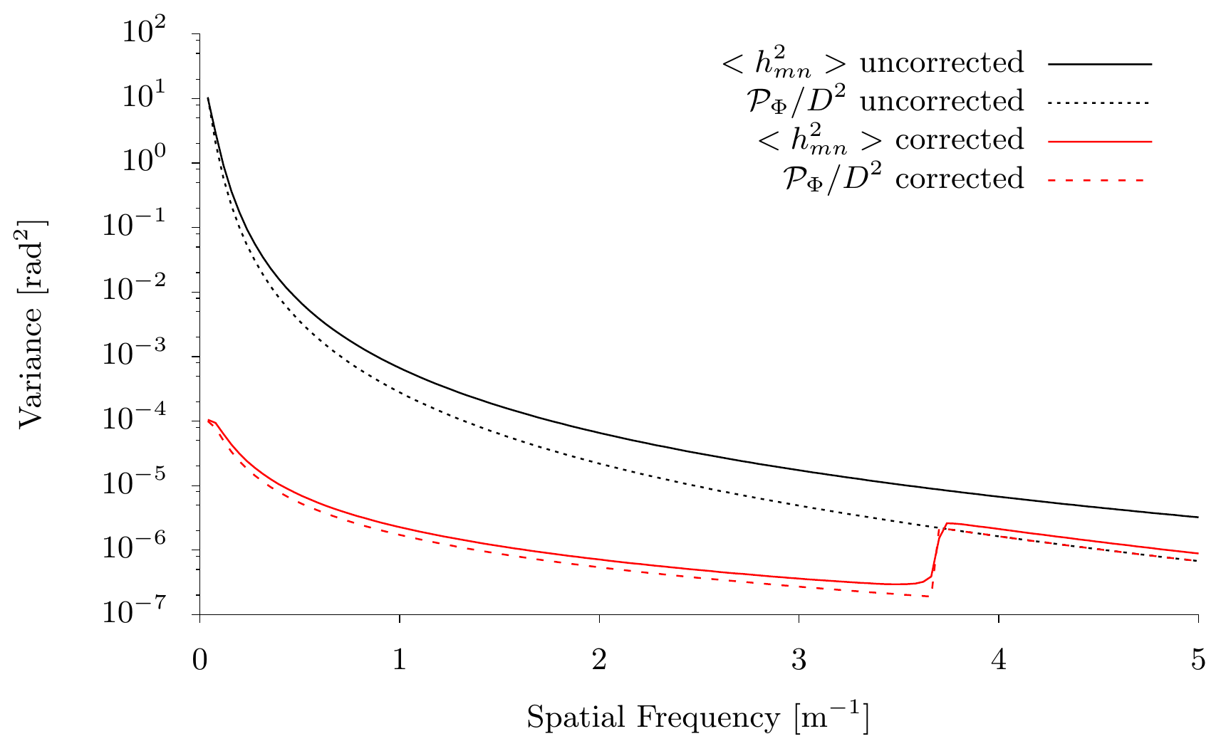
In Figure 1 we show the modal variance vs spatial frequency. This was calculated using numerical integration in
ouble precision with the GNU Scientific Library (GSL \cite{gsl_manual}) routines \\
\verb gsl_integration_qagiu (for the raial integral) and sl_interation_qag (for the azimuthal integral). We found that an absolute tolerance of and a relative tolerance of gave good results.
Figure 1 also shows the naive result using Equation (27). The simple estimate based on the PSD is significantly below the true variance.
One might guess that AO correction will reduce or eliminate this discrepancy. A simple way to estimate the effect of AO control on these statistics is to assume frozen flow and apply a scaling for the time-delay error. Following Guyon[15] (as modified in Appendix B) the corrected PSD is approximated by
| (30) |
where is the wind speed, is the total latency in the control system, and is the actuator spacing projected on the aperture. We next recalculated the modal variances with the corrected PSD, using m/s, ms, and cm on a m aperture.
The variance with and without the aperture is also shown in Figure 1. Though the discrepancy is reduced, the simple estimate based on the PSD is still below the true variance. This means that the variance of a Fourier mode is not simply proportional to the PSD when it is sampled by the aperture.
3.4.3 Correlation
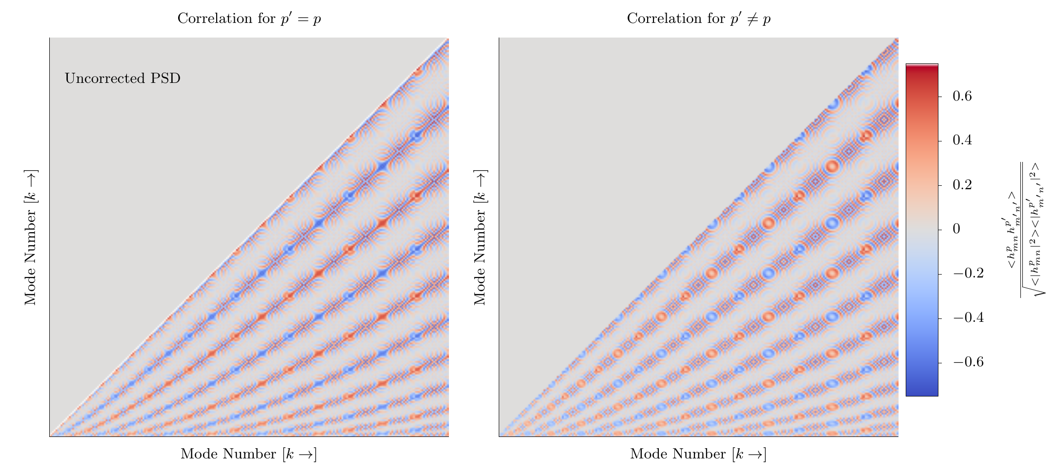
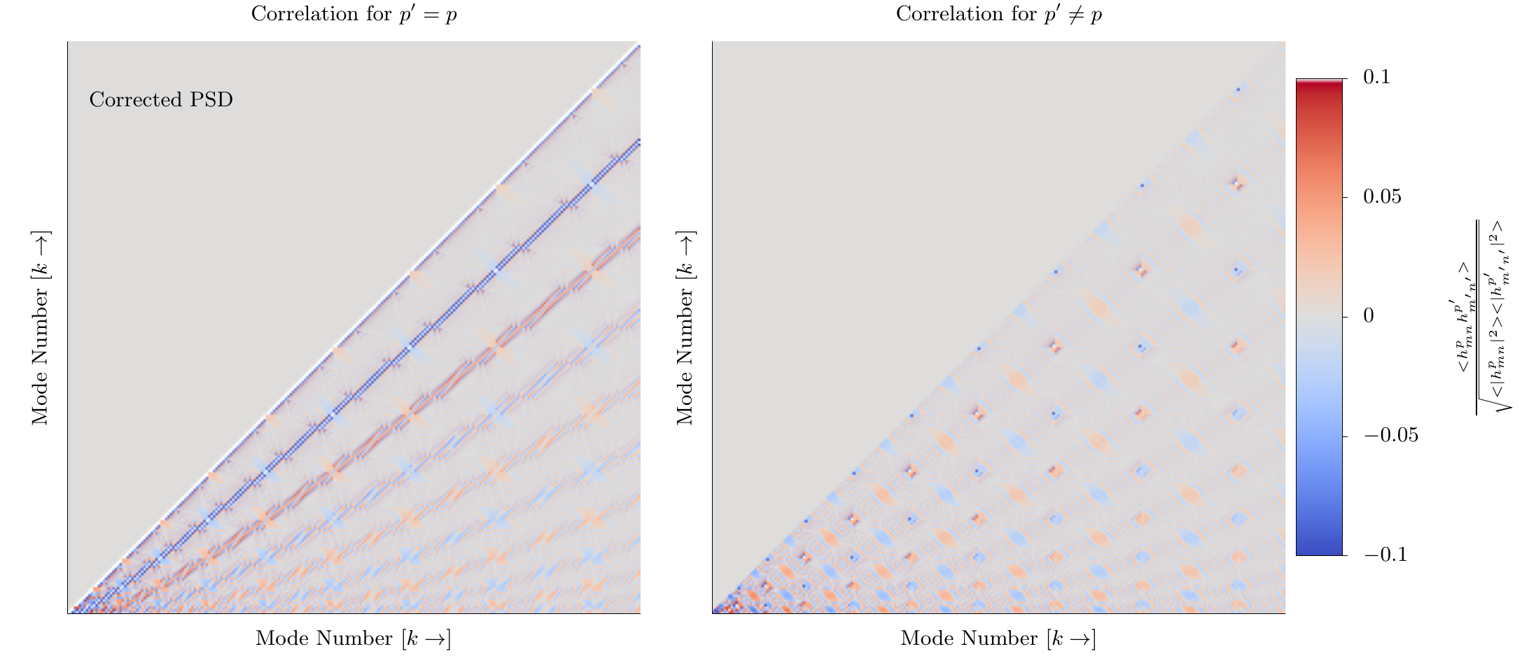
We next calculated the covariance of pairs of Fourier modes according to Equation (25). The results are shown in Figure 2 for uncorrected von Kármán turbulence, and in Figure 3 for the corrected case. In the figure we show the covariances normalized by the modal variances, that is the correlation. There is significant correlation between various modes in the uncorrected case, but an AO system acts to suppress this. In the following section we show that this correlation between Fourier modes can be accounted for by convolving the PSF with the PSD.
4 Post-Coronagraph Contrast
We next derive a PSD-based model of a coronagraph fed by an AO system in the long exposure limit, and assess its validity.
4.1 Coronagraph Model
The intensity in an image plane is given by
| (31) |
The operator describes the propagation of the wavefront from pupil to final image plane. From here on we assume this is the Fourier transform defined as in Appendix A.2, though it could be a series of transforms corresponding to various coronagraph components[27]. We define the system PSF as the result of the above with no aberrations, that is and for all , which is
| (32) |
In the case of the circular unobstructed aperture (Equation 2) this is the Airy pattern
| (33) |
where we have used the image plane coordinate . Telescope apertures are typically more complicated, consisting of secondary mirror obscuration and support structures, possibly segments, and can be non-circular. Furthermore, it could be position dependent due to the coronagraph. The result will be more difficult to analyze, usually requiring numerical calculation.
Equation (31) can not be evaluated in closed form in the general case. However, by assuming small aberrations and an ideal coronagraph we can use a 2nd order Taylor expansion [28, 29] to approximate the post-coronagraph PSF as[30] 111Macintosh et al. [30] only addressed phase, but the extension to amplitude is straightforward from their arguments.
| (34) |
Dealing with the phase component first, we have
| (35) |
Evaluating a single term gives
| (36) |
Then taking the modulus squared and pulling out the terms with gives222We are suppressing the dependence of .
which is the instantaneous intensity at a position and time in the post-coronagraph image plane. Now, we seek the long exposure, or expected, value of this expression. Though this appears quite intractable, we see that this will require evaluating covariances of the form . So, to proceed we make the ansatz that we can temporarily ignore the aperture as in Section 3.4.1. The effect of this assumption is that all covariances are 0, which leads directly to
| (38) |
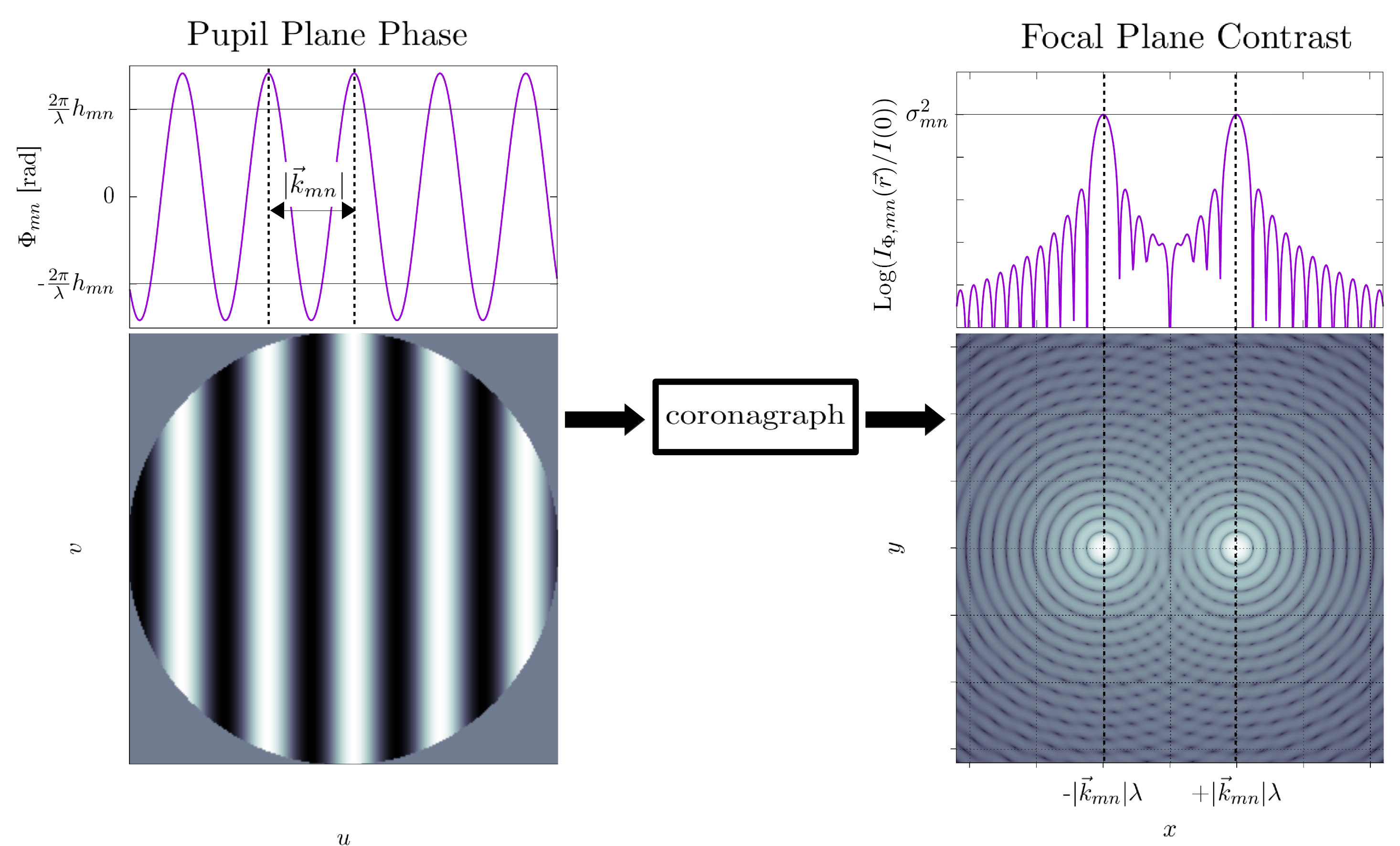
for a single term in the sum on the first line of Equation (4.1). This is the classic result of a Fourier aberration producing a pair of symmetric speckles [31]. We illustrate this in Figure 4.
Finally, we perform the sum over all spatial frequencies. The complete intensity due to at is
| (39) |
This summation is an unnormalized convolution with the PSF, and can be thought of as adding photons from nearby speckles. This step accounts for the effect of the aperture. In the AO corrected regime, it increases the intensity by as much as 50%, explaining the discrepancies in Figure 1.
Now we apply the lesson of Section 3.4.2 above. If we instead use the variance calculated with Equation (28) , then we can skip the convolution and arrive directly at
| (40) |
This is an assertion that the the complete evaluation of Equation 4.1 in the long exposure limit is equivalent to the modal variance calculation on the aperture with Equation 28. Acknowledging that we have not actually proven this, we demonstrate its validity with numerical experiments in the following section.
The amplitude component of the post-coronagraph long-exposure intensity, , is evaluated in nearly identical fashion.
We define the “raw PSF contrast” as the ratio of the intensity at to the peak intensity of a non-coronagraphic long-exposure image of the star, . This is related to the PSF by the long-exposure Strehl ratio , defined by the relationship
| (41) |
The contrast is then
| (42) |
4.2 Numerical Verification
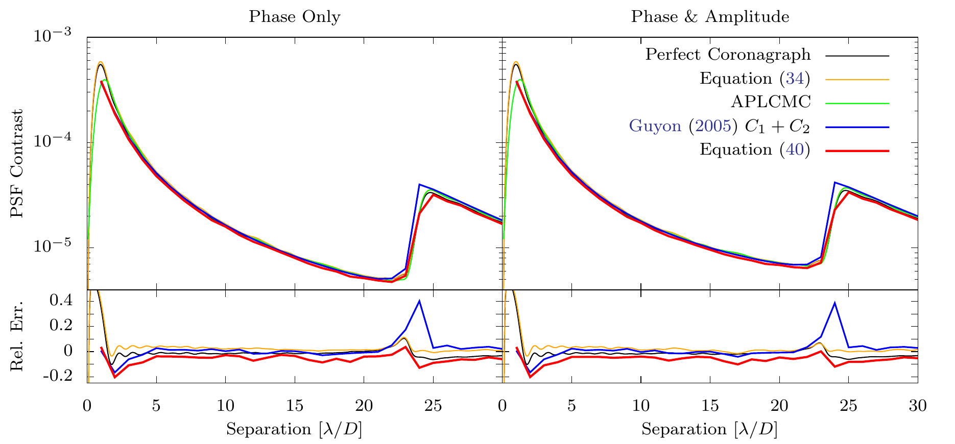
We conducted a set of numerical experiments to verify our long exposure coronagraph model, compare it to other models, and to assess its relevance to real-world coronagraphy. Five distinct model coronagraphs were considered, in each case both for phase aberrations only and with the amplitude errors included.
The first comparison coronagraph model was the so-called “perfect coronagraph” [32]. In this model the complex plane wave which minimizes the energy in the pupil is subtracted, and the result is propagated to the image plane. It has been shown that analysis with the perfect coronagraph produces results which match the real-world Four Quadrant Phase Mask (4QPM) coronagraph [34, 35].
The second coronagraph model consisted of propagating the complex wavefronts using Equation (34) directly, employing the FFT. The phase and amplitude components were treated separately, then combined after taking the modulus squared.
The third coronagraph model corresponds to the measurement error and time delay limited contrast of Guyon[15], combined with the contrast from uncorrected amplitude due to atmospheric scintillation. In Appendix B we present a derivation of utilizing our present notation and generalizing it for arbitrary parameters. This method uses the residual PSD, as in Equation (27), and so requires a convolution. Hence this tests the convolution solution for the discrepancy between the true variance and the simple PSD estimate highlighted above.
The fourth model consisted of directly measuring the variance of each modal coefficient. The coefficient of each mode was measured by inner product with the mean-subtracted phase and amplitude on the aperture for each randomly generated screen. In this case, the aperture is already taken into account so Equation (40) describes the results.
The final comparison coronagraph was an Apodized Pupil Lyot Complex Mask Coronagraph (APLCMC[33]). We included this as an example of a coronagraph which can be implemented in the real world. In this case, the focal plane mask (FPM) was 1.29 in diameter at 800 nm, with a complex transmission of -0.458. The optimum pupil apodization gave a net intensity throughput of 0.587.
We generated a series of phase screens from the von Kármán PSD using Fourier-space convolution of the PSD with Gaussian white noise fields. Scintillation was included by multiplying the PSD by the and functions, Equation (12), resulting in phase and amplitude screens. AO correction of the phase was approximated as in Equation (30). We used a Fried parameter of m, an outer scale m, and windspeed of 10 m/s. The total time delay was set to 2.5 frames at 2000Hz (1.25 ms). We set telescope diameter to m and actuator spacing to cm (48 across), and assumed a wavelength of nm. The phase screens were 2048 pixels across, and we used a circular unobstructed aperture 128 pixels across. We assumed an arbitrarily bright star so WFS measurement noise was ignored. Strehl ratio of a non-coronagraphic image with these parameters was 94%.
10,000 realizations of the AO corrected phase and uncorrected amplitude were generated. For each realization we applied the five comparison coronagraph models. The results for these coronagraphs are shown in Figure 5, where we see that, in general, these various coronagraph models match the APLCMC. We note that the “perfect Coronagraph” and direct propagation using Equation (34) are nearly identical to each other. The residual-PSD+convolution analysis also matches well. So does the direct calculation of modal variance.
4.3 Long-Exposure Contrast and the PSD
We can summarize the results of this section with the following points:
-
•
The post-coronagraph contrast is not simply the residual PSD, due to the effect of the aperture. This is easily addressed by an unnormalized convolution with the PSF.
-
•
If the variance is calculated with the aperture included, then the convolution is not needed.
-
•
Ideal coronagraph models are valid in the regime of ground-based, well-corrected, AO-fed coronagraphy, and are useful proxies for real-world coronagraphs.
Our result that the post-coronagraph long exposure image is a convolution of the PSF with the residual PSD is nearly identical to that developed by Herscovici-Schiller et al. [27] It is fully equivalent if one uses a position dependent PSF and includes internal aberrations, both details we neglect since we are analyzing an ideal system. The difference between this case, and the case when the aperture is included, is important when the modal variances are individually calculated as we do in the following sections.
5 Temporal Power Spectra
Next we describe a process for calculating the temporal PSDs of the Fourier basis in wind-driven von Kármán turbulence.
5.1 Temporal PSD of Fourier Modes in Wind-Driven Turbulence
Re-stating Equation (8), the spatial PSD of a Fourier mode on an unobstructed circular aperture is given by333As noted above, we are suppressing :
| (43) |
We next invoke the Taylor or frozen-flow hypothesis, which for our purposes states that we can treat the time-domain behavior of turbulence as if fixed turbulent phase screens are blowing across the telescope in discrete layers. With this assumption we can calculate the temporal PSD of a turbulent mode with [21, 22]
| (44) |
where is temporal frequency, is the wind-speed, and denotes the temporal PSD of the mode specified by . With no loss of generality we have chosen coordinates such that the wind vector . We have included a factor of 2 since we will consider only .
Now to account for an arbitrary wind direction, let be the direction of the wind with respect to the axis. We then derotate the basis functions by this angle to align with the axes of the integral in Equation (44) by defining
| (45) | ||||
The temporal PSD for arbitrary wind direction is then simply
| (46) |
Finally, the temporal PSD of a Fourier mode for a turbulence profile is the weighted sum of the single layer profiles
| (47) |
5.2 Numerical Calculation
The improper integral in Equation (46) does not in general have a simple closed-form solution, so we must calculate it numerically. In this work we used the GSL sl_interation_qagi 444https://www.gnu.org/software/gsl/manual/html_node/QAGI-adaptive-integration-on-infinite-intervals.html routine. We found that a relative tolerance of and an absolute tolerance of in ouble } precision gave goo results. Though these choices noticeably extend calculation time, less demanding tolerances can produce numerically unsatisfying results. For example, modes with similar spatial frequencies should have similar total variance (integral of the PSD), but setting numerical tolerance too low can introduce occasional 50% jumps.
| Layer | Layer | Layer | Wind | Wind |
| No. | Height1 | Strength2 | Dir3 | Speed |
| [m] | [deg] | [m/s] | ||
| 1 | 250 | 0.42 | 60 | 10 |
| 2 | 500 | 0.03 | 60 | 10 |
| 3 | 1000 | 0.06 | 75 | 20 |
| 4 | 2000 | 0.16 | 75 | 20 |
| 5 | 4000 | 0.11 | 100 | 25 |
| 6 | 8000 | 0.10 | 110 | 30 |
| 7 | 16000 | 0.12 | 100 | 25 |
| Notes: | ||||
| 1Height above the observatory. | ||||
| 2Normalized. | ||||
| 3Angle east of North. | ||||
We also find that temporal frequency sampling is important, settling on Hz as the largest sampling that should be used in general. Larger samplings tend to also produce jumps, caused by moving on and off sharp peaks associated with individual wind-layers. If such a peak falls between two frequencies and the sampling is too coarse, the power in the peak will be missed.
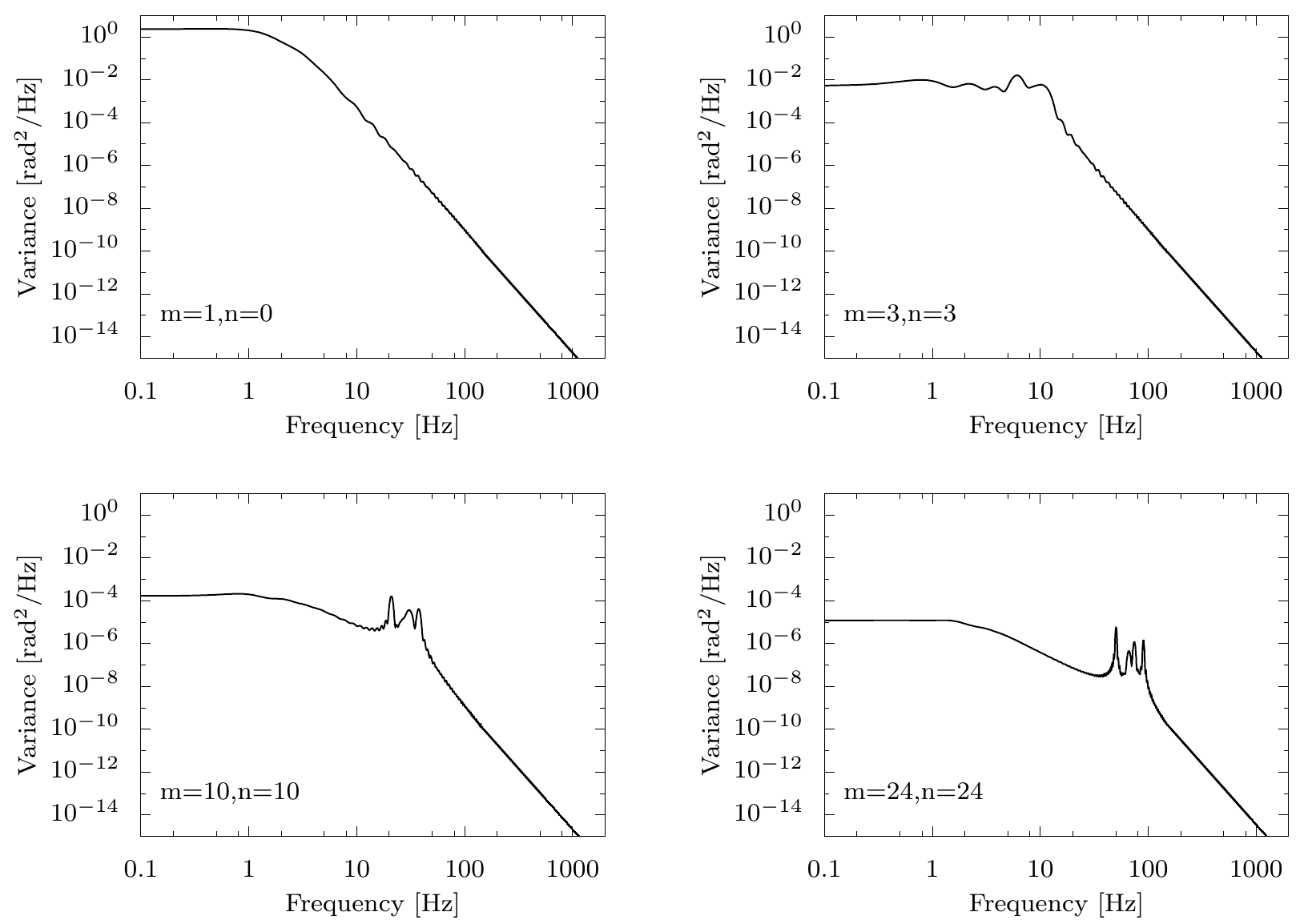
We illustrate calculations of multi-layer turbulence using a seven layer turbulence model based on the Giant Magellan Telescope (GMT) site survey at Las Campanas Observatory (LCO) [36, 37]. The parameters of this profile are given in Table 2. The calculated temporal PSDs for several Fourier modes are shown in Figure 6. Due to the identical wind velocities of several layers, we only expect 4 distinct peaks. The number of peaks seen at a given spatial frequency depends on . If the frequency of two peaks are not well separated they appear blended at the resolution of the calculations and plots.
5.3 Temporal PSD of Measurement Noise
We also need the PSD of the WFS measurement noise. The variance at a spatial frequency due to photon noise in the wavefront sensor is[15]
| (48) |
where the factor quantifies the sensitivity of the WFS to photon noise. is the total number of photons available for wavefront sensing:
| (49) |
where is the photon rate (photons sec-1) sensed by the WFS, and is the integration time of the WFS. depends on star brightness through
| (50) |
Where is the Vega magnitude of the star in the WFS bandpass, and is the photon rate of a 0 star in the WFS bandpass including total system throughput. Here we expand this to include background and readnoise. The signal-to-noise ratio is
| (51) |
where is the number of pixels involved in measuring , each pixel having readout noise with variance , and is the photon rate per pixel from the background. Now the WFE due to photon noise at the WFS wavelength can be written as
| (52) |
This variance is spread over the sampling bandwidth of the WFS, . We can determine the temporal PSD of measurement noise from
| (53) |
assuming white noise (a flat PSD) we have
| (54) |
Note that in the absence of detector noise, is independent of .
6 Closed Loop Control
Now that we have established the temporal PSDs of the Fourier modes and of WFS measurement noise, we can use them to predict the residual wavefront variance in a closed-loop AO system. Here we follow the standard model used throughout the AO literature, and so only briefly introduce the concepts and our notation. Note that though here we apply the following to the frozen-flow turbulence PSDs we just derived, the techniques are general and could be applied to PSDs in any basis set and to PSDs including additional error sources such as telescope vibrations and non-frozen-flow.
6.1 Transfer Functions
First we need the error and noise transfer functions of the AO control system. Here we closely follow the development of Poyneer et al.[38], and see also the treatment by Madec[39]. Our goal is to calculate the error transfer function (ETF) of the control system, which is defined as
| (55) |
That is, the ETF describes the AO system as a temporal filter which acts on the input PSD. The noise transfer function (NTF) is similarly defined, except that it acts on the measurement noise PSD. The ETF and NTF are constructed using the frequency responses, or transfer functions, of the various components of the system, which we will denote as .
The WFS measurement is an average of the turbulence over the integration time. Likewise, the deformable mirror (DM) is assumed to move in discrete steps, holding its position between updates. The frequency response of such components is called a sample and hold, which has the functional form
| (56) |
where , being the loop sampling frequency, and . There will be a delay due to sensor readout, data transfer, calculations, etc.555It is common to discuss the “total delay” including 1/2 the WFS sample and hold (for the mid-point of the integration), and 1/2 the DM sample and hold. That is the total delay is [39]., which has a transfer function
| (57) |
The system forms an estimate of the coefficient of a mode, . In closed-loop the WFS measures the change in the coefficient of a given mode, . This is combined with the current estimate of the total coefficient to form a new estimate of , which is then applied to the DM. At time-step the coefficient is specified in terms of the current and previous and , by a linear combination
| (58) |
where is the loop gain. Below we consider in depth how to choose the parameters of this control filter. The frequency response of this general linear filter is [40]
| (59) |
and we can map from the -domain to the -domain by the substitution .
With the above component frequency responses, we can write the open-loop ETF as
| (60) |
From this it follows that the closed-loop ETF is
| (61) |
The closed-loop noise transfer function (NTF) is
| (62) |
The residual PSD in closed-loop control is then the product of the modulus-squared ETF and the modal PSD, and the modulus-squared NTF and WFS noise PSD:
| (63) |
The residual variance in this mode is just the integral of the residual PSD:
| (64) |
Note that, since we started with Equation (43), this estimate of the variance explicitly includes the aperture and so directly describes the post-coronagraph intensity.
To employ these calculations, we next need to determine the parameters of Equation (58) and then find the optimum gain.
6.2 Control Laws
Our next step in analyzing a closed-loop AO system is to choose the control law used to feed WFS measurements back to the DM. Here we analyze two: the simple integrator and the Linear Predictor.
6.2.1 Simple Integrator
At time step , the WFS measures the residual wavefront, . We combine this with the last estimate, , which is the result of the previous cycle. The simplest estimate at the current step is the simple integrator (SI)
| (65) |
This corresponds to a choice of and in Equation (58). It is also common to choose (slightly), a so-called leak term, making this the “leaky integrator” control law. Here we will confine our analysis to the SI control law.
6.2.2 Linear Predictor
In general the estimate formed by the SI controller will be slightly incorrect when actually applied due to the finite loop delay. Here we consider a conceptually straightforward extension of the integrator to include a prediction. We note that more sophisticated methods exist, which we discuss after presenting our results.
One way to improve the accuracy of the estimate formed by the controller is with a filter of the form
| (66) |
We can determine a set of which are optimal in the least-squares sense from the temporal autocorrelation of the modal amplitude, , where is the lag, by solving the Normal or Yule-Walker equations [41, 40]:
| (67) |
where
| (68) |
and
| (69) |
We can find the autocorrelation of the time-series of a mode from its PSD using the Wiener-Khinchin theorem [42], which states that the autocorrelation is the Fourier transform of the PSD:
| (70) |
In Appendix C we give a recipe for calculating the autocorrelation from a numerical PSD.
The solution vector contains the optimal Linear Predictor (LP) coefficients, which minimize the least-squares error of the output of Equation (66). The matrix is a symmetric Toeplitz matrix, and so the Normal equations can be solved very efficiently using Levinson’s recursion [43](chapter 2). A nice result of using Levinson’s recursion to solve the Yule-Walker equations is that the resultant filter is guaranteed to be stable [41].
To apply the LP in closed-loop, we use as the coefficients in Equation (58). That is, , and , . We can then to determine the optimal loop gain .
6.3 Gain Optimization
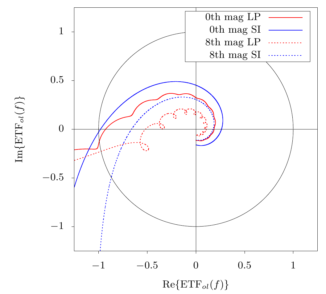
All that remains is to describe how to choose the optimum value of the gain. The first step is to identify the maximum stable gain, , which is the value of at which the system becomes unstable666This is sometimes called the “ultimate gain”.. Following Dessenne et al.[44] we evaluate stability of the control law using a Nyquist plot of the open-loop ETF, which plots the real and imaginary components of Equation (60). In this plane, as long as the ETF does not encircle the point (0,-1), then the system is stable – a result known as Nyquist’s stability criterion. We then can find the value of by finding the value of which causes the curve to intersect (0,-1). This is illustrated in Figure 7.
From here we follow the standard recipe [45, 25] for using the input (or “open-loop”) PSD to optimize the closed-loop gain. The per-mode variance-minimizing optimum gain is given by solving:
| (71) |
This is a straightforward optimization problem, which we solve using Brent’s method as implemented in the boost c++ library.
7 Closed Loop Contrast Calculations
Given the temporal PSD, the ETF and NTF, and the optimal gain, equation (64) describes the residual variance at a given spatial frequency in a closed-loop AO system. We showed how this is related directly to the PSF contrast behind a coronagraph in Section 4. So, calculating the closed-loop long-exposure post-coronagraph contrast consists of the following steps:
- 1.
-
2.
Calculate the temporal PSD of measurement noise according to Section 5.3.
- 3.
-
4.
Determine the ETF and NTF per Section 6.1
-
5.
Populate the residual PSD as follows:
(72) - 6.
-
7.
Calculate the long-exposure Strehl ratio as the sum of variance over all spatial frequencies to find and use the extended Marechal approximation
(73) -
8.
Calculate the contrast according to Equation (42).
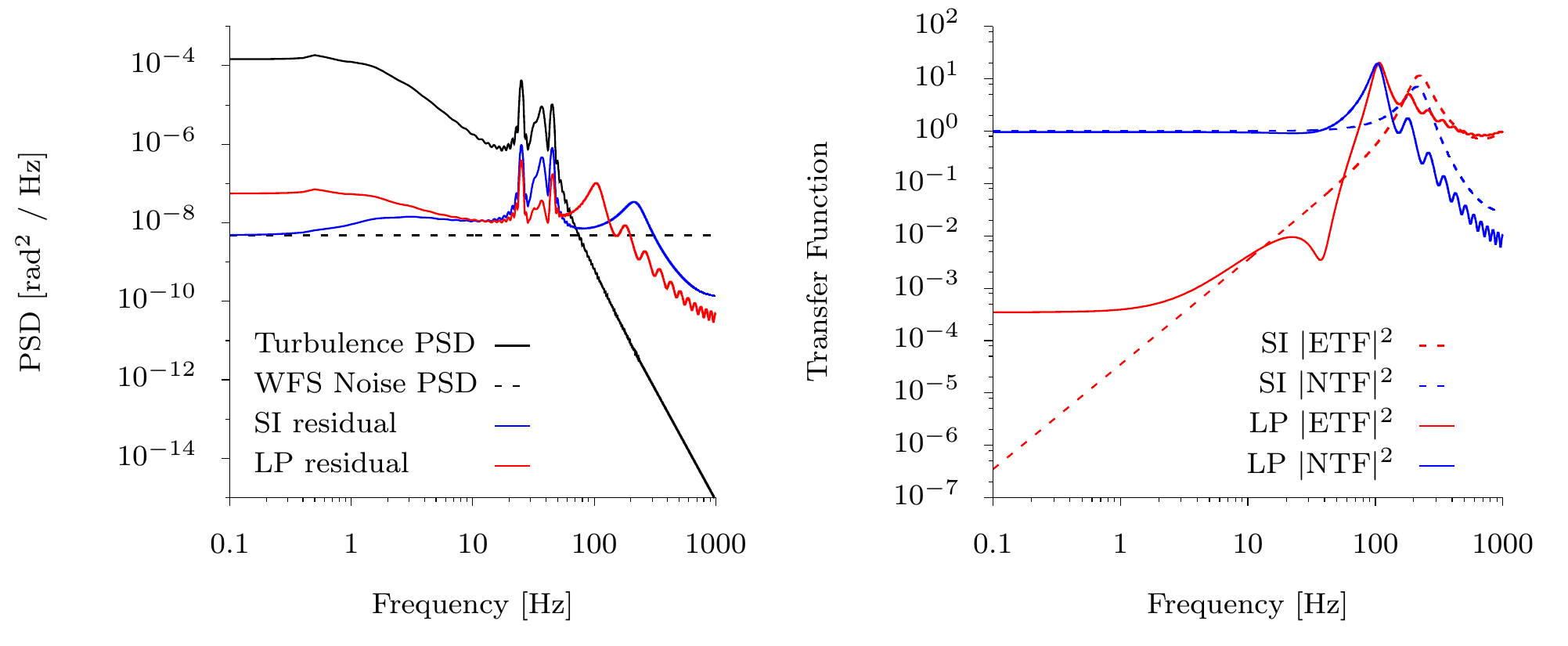
The first four steps are illustrated in Figure 8. The PSD of a Fourier mode is shown in the left-hand panel. The gain-optimized ETFs and NTFs, for both SI and LP controllers, are shown in the right-hand panel. The left-hand panel also shows the residual PSDs after applying the ETFs and NTFs to the input turbulence PSD.
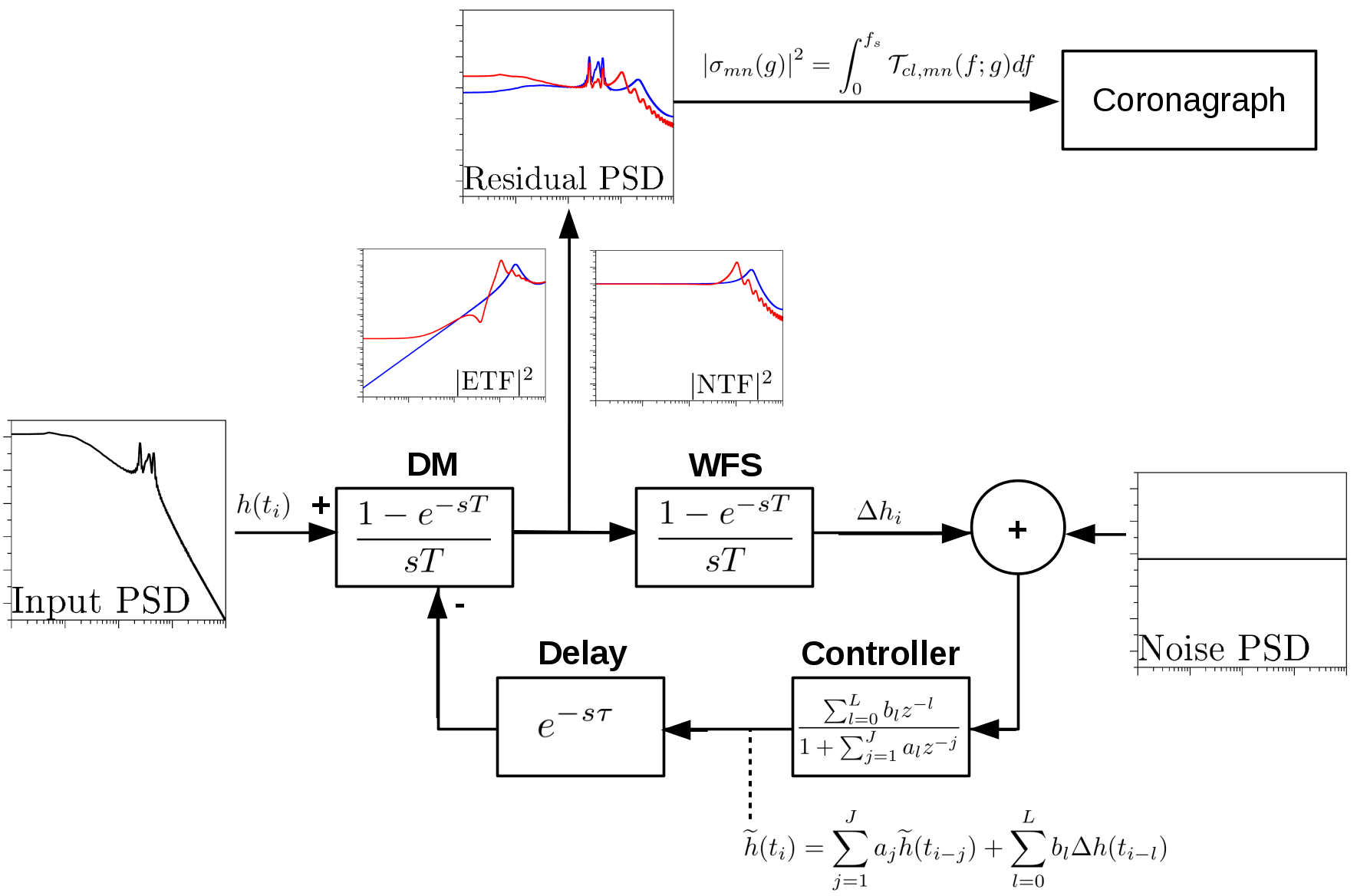
We illustrate the complete framework in Figure 9. The frequency response of each component is applied to the input PSD, and to the noise PSD, according to the ETF and NTF. The output residual PSD is then input to the coronagraph.
We applied our method to the cases of a 6.5 m circular aperture, here motivated by the in-development MagAO-X system [47]. We also consider a 25.4 m telescope, for which we used the collecting area of the GMT (seven 8.4 m segments), but ignored details of the aperture in PSD and contrast calculations. The parameters of our calculations for these telescopes are listed in Table 3.
| Symbol | Parameter | Value | Units | Notes |
| Max sampling frequency | 2000 | Hz | ||
| Loop delay | 1.5 | frames | ||
| Actuator spacing | 0.135 | m | 48 across 6.5 m | |
| WFS Sensitivity | For unmodulated pyramid | |||
| WFS Wavelength | 800 | nm | Based on the MagAO WFS [48] | |
| WFS Filter Width | 357 | nm | Based on the MagAO WFS [48] | |
| WFS Throughput | 0.1 | [ratio] | ||
| WFS Exposure Time | 0.0005 | s | 2 kHz | |
| WFS Readout noise | 0.1 | electrons | ||
| 0 mag flux density @ 800 nm | photons/sec/m2/nm | Vega based. | ||
| Sky background @ 800 nm | 20 | mags/arcsecond2 | ||
| Fried Param. | 0.16 | m | Median 0.62” at m [37] | |
| Weighted mean wind speed | 18.7 | m/s | moment [19] | |
| Magellan Clay | ||||
| Telescope Diameter | 6.5 | m | ||
| 0 mag Photon Flux | photons/sec | Unobstructed aperture | ||
| WFS Pixels | 7280 | pixels | 4 quadrants with D/d across | |
| Background flux | 0.22 | photons/pix/sec | Assumes 2” FOV for WFS | |
| GMT | ||||
| Telescope Diameter | 25.4 | m | Edge to edge | |
| 0 mag Photon Flux | photons/sec | Vega, using GMT aperture | ||
| WFS Pixels | 111,208 | pixels | 4 quadrants with D/d across | |
| Background flux | 0.01 | photons/pix/sec | Assumes 2” FOV for WFS | |
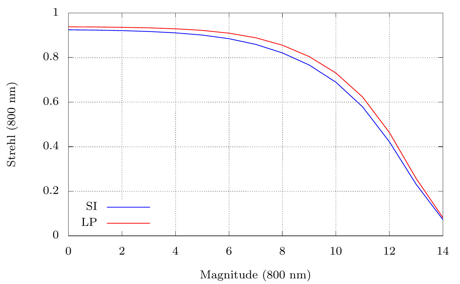
Figure 10 shows the Strehl ratio vs. guide star magnitude predicted for the 6.5 m AO system at 800 nm. Only residual turbulence is accounted for, including the uncorrected power (a.k.a. fitting error).
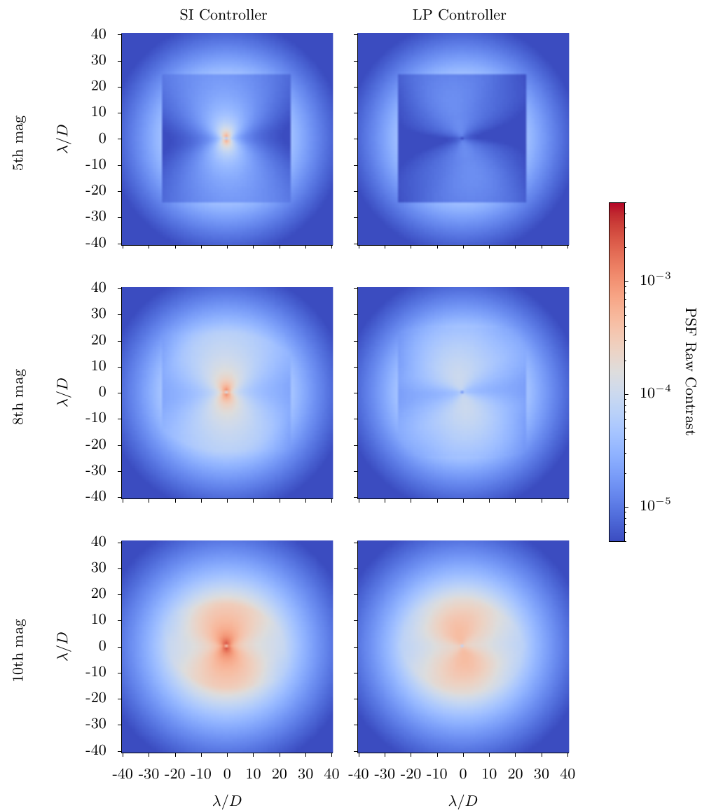
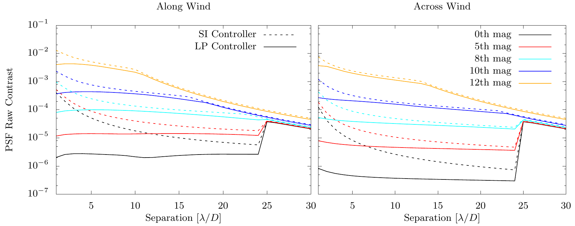
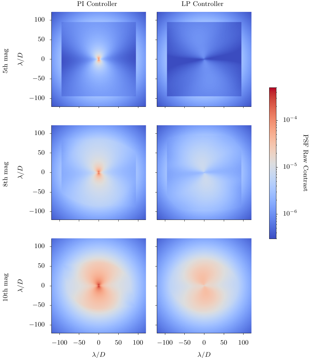
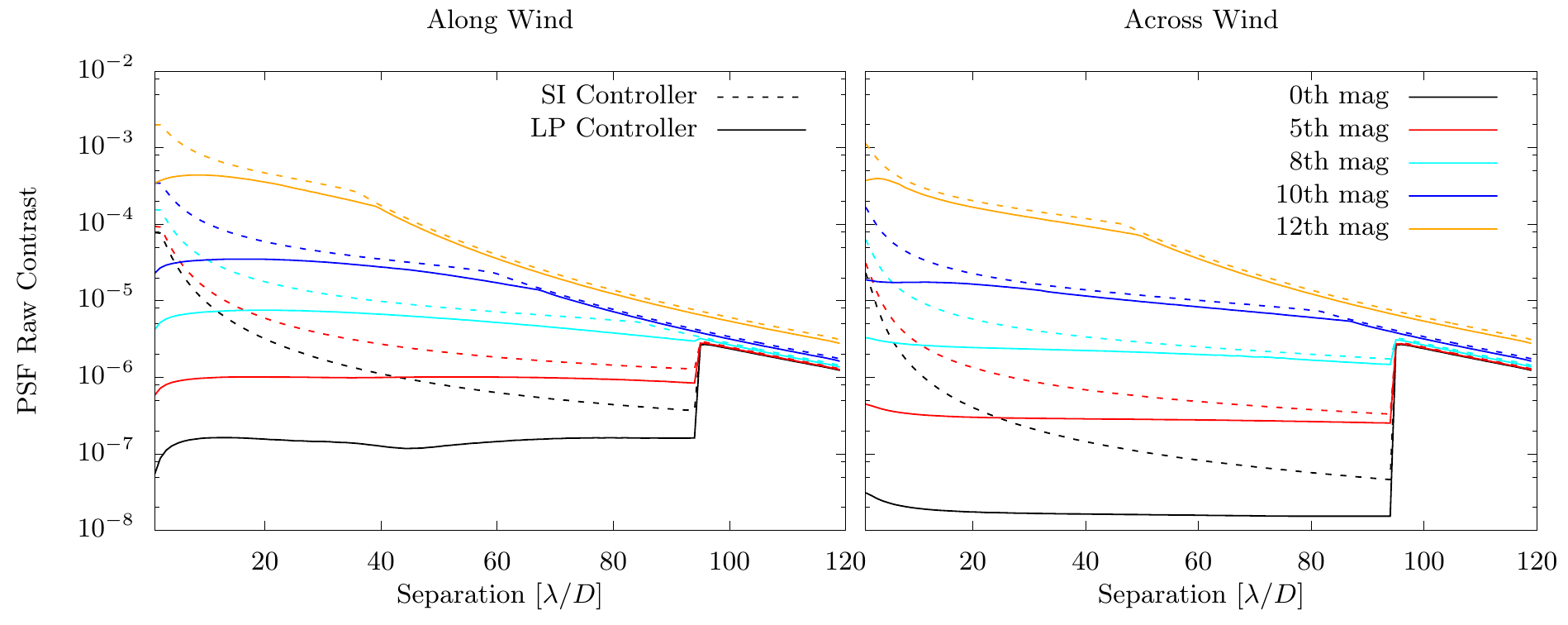
In Figure 11 we show the contrast maps for the 6.5 m system observing 5th, 8th, and 10th magnitude stars, for both controllers at the WFS wavelength. To estimate the PSF contrast at other wavelengths all of these results can be scaled by . The figure shows, as expected, deeper contrasts on brighter stars. The SI controller (left hand column) exhibits the well known “wind butterfly”, and we see that the gain optimization process turns off modes on fainter stars, changing the shape of the dark hole. The LP controller does not show the “wind butterfly”, rather predictive control essentially eliminates it. It also results in deeper contrasts. Figure 12 shows the PSF contrast profiles both along and across the wind direction.
The same calculations were made for the 25.4 GMT-like telescope, shown in Figures 13 and 14. The results are qualitatively similar, but show a nearly improvement due to the larger aperture. This can be understood as the larger diameter causing the spatial-frequency sampling interval, , to impose less power per , resulting in less residual power per mode.
For both the 6.5 m and the 25.4 m telescopes, the gain in contrast at small separations provided by the LP controller is remarkable. On the 6.5 m observing a 0 mag star, the LP contrast is over 200 times better at 1 , and is nearly 10 times better for an 8th mag star. On the 25.4 m the LP contrast is over 1400 times better at 1 on a 0 mag star, and is over 30 times better for an 8th mag star.
8 Discussion
8.1 Predictive Control
Predictive control has been discussed in many other studies. Here we used a relatively simple form of it, rather than more sophisticated options. The LP controller provides a conceptually simple extension of the integrator controller, and provides an efficient and easy to understand method for calculating its coefficients since we know the open-loop PSD. However, it is not the most sophisticated method proposed to-date in the literature and our intent here is not to propose it as the best one.
Dessenne et al. [44, 49] presented a method using a linear filter, essentially identical to the technique we used. Their method for optimizing the parameters was based on an explicit least squares minimization using past data, rather than the PSD, and allowed the coefficients and to differ. This technique was demonstrated on sky.
We recently presented a related predictive control strategy, based on empirical orthogonal functions (EOFs)[50]. EOFs are essentially a time-and-space Karhunen-Loève basis, and this method allows for including non-WFS measurements, such as accelerometers. Filter optimization is done on past time-domain data. We found essentially the same level of improvement in simulations.
Johnson et al. [51] developed a control strategy based on predicting the wind-driven translation of turbulent layers. With simulations incorporating on-sky data from the ViLLaGEs AO system [52] they showed significant increase in Strehl on fainter stars, and predicted large gains in Strehl for larger telescopes.
Much recent work has been in the area of linear quadratic Gaussian (LQG) controllers. Poyneer et al.[24] proposed a Fourier-mode by Fourier-mode optimization of a Kalman filter controller, and using end-to-end simulations showed large gains in contrast similar to what we have shown. They presented their method as a control filter much as we did here. They pointed out that any filter could be cast in the direct form as in Equation (59), though it is then subject to errors due to numerical precision if actually used to implement the filter.
More broadly, the determination of optimum control filters is of great interest in the AO-related literature. In the context of AO this has been studied extensively for LQG controllers [53, 54]. See also the review of various system identification strategies presented in Kulcsár et al.[55]
While this paper was under review, Correia et al. presented an analysis of predictive control using the distributed Kalman filter method[14]. Their analysis employed the spatial filtering method (as opposed to our temporal frequency method), and showed post-coronagraph contrast gains for the Keck AO system at least as large as we show here.
Any of these control methods can be represented by their temporal transfer functions, and so could be included in further studies using our technique. In summary, the LP is not the only, nor the most advanced, technique we have available, but it is apparent that predictive control offers significant gains for high contrast imaging of exoplanets.
8.2 Sensitivity to Frozen Flow
Our model of input turbulence was based on the frozen flow model. However, our semi-analytic method does not require frozen flow. That is, any source of the temporal PSDs could be used as input to the analysis. We could incorporate boiling, or disturbances derived from telescope models (e.g. vibrations due to wind shake). This could also be extended to assess the impact of time-variable turbulence profiles.
It should be expected that inclusion of additional sources of error will reduce projected performance. In the case of, e.g., telescope vibrations this is simply because there is more variance in the system. In the case of time-variable turbulence, i.e. changing wind and seeing, the reduced performance will result from sub-optimality of the filter coefficients.
8.3 Impact on Exoplanet Characterization
Our motivation for this study was to analyze the limits of ground-based coronagraphic exoplanet characterization, and to assess the impact that predictive control will have on it. Consider the coupling of an ExAO-fed coronagraph to a high-dispersion spectrograph[56], a technique recently dubbed “high dispersion coronagraphy” (HDC) [57, 58]. We focus on this technique because it is, in principle, photon-noise limited, meaning we do not have to consider speckle noise. Neglecting detector and background noise, the signal-to-noise ratio (S/N) in the HDC technique is given by [56]
| (74) |
Where is the photon rate from the planet and is the photon rate from the star (both in one spectral resolution element), and is the number of resolved lines in the planet spectrum used for cross-correlation template matching. is the raw PSF contrast as we have derived here. is the integration time needed to reach a desired S/N. This leads directly to
| (75) |
So, in terms of required integration times the potential benefits of predictive control are quite profound. Using just the relatively simple form of it considered in this study, we find that predictive control of atmospheric turbulence could make a GSMT up to 30 times more efficient at exoplanet characterization around a star as bright as Proxima Centauri, and up to 1400 times more efficient on brighter stars.
8.4 Code Availability
The code we developed for this analysis is freely available at https://github.com/jaredmales/aoSystem. It is written in ++ , is highly parallelized, and ompiles to a command line application which accepts configuration files to set up the analysis. It depends on the library available at https://github.com/jaredmales/mxlib, as well as several easily available open-source libraries. No licenses are needed.
9 Conclusion
We have developed a semi-analytic framework for predicting the raw PSF contrast in an AO-fed coronagraphic image under closed-loop control. Instead of the usual spatial-filter analysis, we explicitly calculated temporal PSDs and analyzed AO performance in the temporal-frequency domain. Our technique takes into account closed-loop dynamics as well as a multi-layer frozen-flow turbulence model. We also analyzed performance of ideal coronagraphs, showing how to account for the subtle difference between the residual PSD and the residual modal variance on an aperture. Using our model, we showed that predictive control will improve raw contrast by up to a factor of 1400 on bright stars, and by a factor of 30 on 8th magnitude stars, compared to the simple integrator control law. Assuming a photon-noise limited observation, the exposure time required to characterize an exoplanet will decrease by the same large factors. This has significant implications for the potential of the coming ground-based GSMTs to search for life outside our Solar System, and makes predictive control one of the key techniques that must be perfected for exoplanet characterization.
10 Acknowledgements
This work was motivated by a question from Marcos van Dam. We thank Richard Frazin for reviewing an early draft of this manuscript. We thank the two anonymous referees for their careful and insightful reviews which significantly improved this manuscript. Early steps in this work were performed under contract with the California Institute of Technology (Caltech)/Jet Propulsion Laboratory (JPL) funded by NASA through the Sagan Fellowship Program executed by the NASA Exoplanet Science Institute. The authors acknowledge support from NSF awards 1506818 and 1625441.
Appendix A Mathematics of the Fourier Basis
We derive the normalizations and Fourier transforms of the Fourier basis on a circular aperture.
A.1 Normalization
The norm of the cosine mode on the aperture is
| (A.1) |
For a symmetric aperture, we can restrict ourselves to with no loss of generality, which simplifies the integral to
| (A.2) |
Using the exponential form of the cosine
| (A.3) |
With the following identity
| (A.4) |
(cf. [59] 8.411 #7), the integral evaluates as
| (A.5) |
Next using the identity
| (A.6) |
(cf. [59] 5.52 #1) and a change of variables we have
| (A.7) |
Similarly, the norm of the sine mode on the aperture is
| (A.8) |
and the norm of the product is
| (A.9) |
A.2 Fourier transforms on an aperture
We need the Fourier transform of the Fourier modal basis over the aperture of the telescope, that is
| (A.10) |
The unobstructed circular aperture is described by Equation (2).
Now switching to polar coordinates and collecting terms we have
| (A.11) |
where we have made use of the complex exponential form of the cosine. We next introduce the notational simplification
| (A.12) | ||||
and the associated angles defined by
| (A.13) | ||||
The transform can now be written
| (A.14) |
With the following identity
| (A.15) |
(cf. [59] 8.411 #7) the transform is equivalent to
| (A.16) |
where are the cylindrical Bessel functions of the first kind. With the identity
| (A.17) |
(cf. [59] 5.52 #1) we finally have
| (A.18) |
Similarly for the sine modes
| (A.19) |
Appendix B Contrast of Guyon (2005)
Here we present a derivation of the contrast due to time delay and measurement error from [15], there called . We extend the analysis of [15] to include finite loop delays, detector and background noise, and make it consistent with the results of Section 4. A spatial frequency component of the wavefront phase at time can be written as
| (B.1) |
where the coefficient is the combined amplitude of the Fourier mode, and is its phase. The superscript is to differentiate this unnormalized basis from the normalized Fourier modes presented in Section 3.3.1. Now at a time later the wavefront will be
| (B.2) |
The residual variance after applying the wavefront correction will be
| (B.3) |
which becomes
| (B.4) |
We next employ the frozen flow hypothesis, assuming that the amplitude does not change and that the phase changes only due to wind-driven flow. This gives
| (B.5) | ||||
which leads to the residual variance due to time lag
| (B.6) |
Now the variance of each mode will be given by the spatial PSD according to
| (B.7) |
Employing the wavefront variance from measurement noise given by Equation (52), the total residual variance at the science wavelength will be
| (B.8) |
In this open-loop framework, the equivalent time lag is where is the closed loop delay defined in Section 6.1, and accounts for the sample-and-hold of the WFS and DM [39]. We calculate the optimum frame rate which minimizes the variance by differentiating Equation (B.8) with respect to , which yields a quartic equation
| (B.9) |
Each mode will have its own optimum , which is somewhat analogous to modal gains in closed-loop control. Since , we can use the results of Section 4 to write
| (B.10) |
The summation in Equation (39) defines , which leads to the expression for the contrast
| (B.11) |
The Strehl ratio can be calculated by summing the total WFE after the convolution and then employing the Marechal approximation
| (B.12) |
It is straightforward to derive the other contrasts, , of [15] using similar arguments.
Appendix C Calculating the Autocorrelation
The autocorrelation can be calculated from a numerical PSD using the following recipe:
1. Start with temporal PSD at discrete frequencies , where and .
2. Form the two-sided temporal PSD of length by augmenting with 0 at the beginning, and augmenting with the reverse at the end:
| (C.1) |
3. Calculate the DFT of the augmented PSD using the FFT algorithm, giving the autocorrelation at lag
| (C.2) |
Note that this is will be a circular autocorrelation wrapping around after points. should be chosen to be larger (by at least a factor of 2) than the needed number of points of .
4. The lags of the points are given by
| (C.3) |
where only the first points are unique.
References
- [1] G. Anglada-Escudé, P. J. Amado, J. Barnes, et al., “A terrestrial planet candidate in a temperate orbit around Proxima Centauri,” Nature 536, 437–440 (2016).
- [2] C. Lovis, I. Snellen, D. Mouillet, et al., “Atmospheric characterization of Proxima b by coupling the SPHERE high-contrast imager to the ESPRESSO spectrograph,” A&A 599, A16 (2017).
- [3] O. Guyon, F. Martinache, E. J. Cady, et al., “How ELTs will acquire the first spectra of rocky habitable planets,” in Adaptive Optics Systems III, Proc. SPIE 8447, 84471X (2012).
- [4] J. R. Males, L. M. Close, O. Guyon, et al., “Direct imaging of exoplanets in the habitable zone with adaptive optics,” in Adaptive Optics Systems IV, Proc. SPIE 9148, 914820 (2014).
- [5] W. J. Borucki, D. Koch, G. Basri, et al., “Kepler Planet-Detection Mission: Introduction and First Results,” Science 327, 977 (2010).
- [6] C. D. Dressing and D. Charbonneau, “The Occurrence of Potentially Habitable Planets Orbiting M Dwarfs Estimated from the Full Kepler Dataset and an Empirical Measurement of the Detection Sensitivity,” ApJ 807, 45 (2015).
- [7] G. D. Mulders, I. Pascucci, and D. Apai, “A Stellar-mass-dependent Drop in Planet Occurrence Rates,” ApJ 798, 112 (2015).
- [8] X. Bonfils, N. Astudillo-Defru, R. Díaz, et al., “A temperate exo-Earth around a quiet M dwarf at 3.4 parsecs,” ArXiv e-prints (2017).
- [9] J. A. Dittmann, J. M. Irwin, D. Charbonneau, et al., “A temperate rocky super-Earth transiting a nearby cool star,” Nature 544, 333–336 (2017).
- [10] M. Gillon, A. H. M. J. Triaud, B.-O. Demory, et al., “Seven temperate terrestrial planets around the nearby ultracool dwarf star TRAPPIST-1,” Nature 542, 456–460 (2017).
- [11] F. J. Rigaut, J.-P. Veran, and O. Lai, “Analytical model for Shack-Hartmann-based adaptive optics systems,” in Adaptive Optical System Technologies, D. Bonaccini and R. K. Tyson, Eds., Proc. SPIE 3353, 1038–1048 (1998).
- [12] B. L. Ellerbroek, “Linear systems modeling of adaptive optics in the spatial-frequency domain,” Journal of the Optical Society of America A 22, 310–322 (2005).
- [13] L. Jolissaint, J.-P. Véran, and R. Conan, “Analytical modeling of adaptive optics: foundations of the phase spatial power spectrum approach,” Journal of the Optical Society of America A 23, 382–394 (2006).
- [14] C. M. Correia, C. Z. Bond, J.-F. Sauvage, et al., “Modeling astronomical adaptive optics performance with temporally filtered Wiener reconstruction of slope data,” Journal of the Optical Society of America A 34, 1877 (2017).
- [15] O. Guyon, “Limits of Adaptive Optics for High-Contrast Imaging,” ApJ 629, 592–614 (2005).
- [16] I. J. M. Crossfield, “On high-contrast characterization of nearby, short-period exoplanets with giant segmented-mirror telescopes,” A&A 551, A99 (2013).
- [17] C. Vérinaud, M. Le Louarn, V. Korkiakoski, et al., “Adaptive optics for high-contrast imaging: pyramid sensor versus spatially filtered Shack-Hartmann sensor,” MNRAS 357, L26–L30 (2005).
- [18] L. A. Poyneer and B. Macintosh, “Spatially filtered wave-front sensor for high-order adaptive optics,” Journal of the Optical Society of America A 21, 810–819 (2004).
- [19] J. W. Hardy, Adaptive Optics for Astronomical Telescopes (1998).
- [20] D. L. Fried, “Statistics of a Geometric Representation of Wavefront Distortion,” Journal of the Optical Society of America (1917-1983) 55, 1427–1431 (1965).
- [21] F. Roddier, M. J. Northcott, J. E. Graves, et al., “One-dimensional spectra of turbulence-induced Zernike aberrations: time-delay and isoplanicity error in partial adaptive compensation,” Journal of the Optical Society of America A 10, 957–965 (1993).
- [22] J.-M. Conan, G. Rousset, and P.-Y. Madec, “Wave-front temporal spectra in high-resolution imaging through turbulence.,” Journal of the Optical Society of America A 12, 1559–1570 (1995).
- [23] R. J. Noll, “Zernike polynomials and atmospheric turbulence,” JOSA 66, 207–211 (1976).
- [24] L. A. Poyneer, B. A. Macintosh, and J.-P. Véran, “Fourier transform wavefront control with adaptive prediction of the atmosphere,” Journal of the Optical Society of America A 24, 2645 (2007).
- [25] L. A. Poyneer and J.-P. Véran, “Optimal modal Fourier-transform wavefront control,” JOSAA 22, 1515–1526 (2005).
- [26] M. Galassi et al., GNU Scientific Library Reference Manual, 3rd ed. (2016).
- [27] O. Herscovici-Schiller, L. M. Mugnier, and J.-F. Sauvage, “An analytic expression for coronagraphic imaging through turbulence. Application to on-sky coronagraphic phase diversity,” MNRAS 467, L105–L109 (2017).
- [28] A. Sivaramakrishnan, J. P. Lloyd, P. E. Hodge, et al., “Speckle Decorrelation and Dynamic Range in Speckle Noise-limited Imaging,” ApJ Letters 581, L59–L62 (2002).
- [29] M. D. Perrin, A. Sivaramakrishnan, R. B. Makidon, et al., “The Structure of High Strehl Ratio Point-Spread Functions,” ApJ 596, 702–712 (2003).
- [30] B. Macintosh, L. Poyneer, A. Sivaramakrishnan, et al., “Speckle lifetimes in high-contrast adaptive optics,” in Astronomical Adaptive Optics Systems and Applications II, R. K. Tyson and M. Lloyd-Hart, Eds., Proc. SPIE 5903, 170–177 (2005).
- [31] F. Malbet, J. W. Yu, and M. Shao, “High-Dynamic-Range Imaging Using a Deformable Mirror for Space Coronography,” PASP 107, 386 (1995).
- [32] C. Cavarroc, A. Boccaletti, P. Baudoz, et al., “Fundamental limitations on Earth-like planet detection with extremely large telescopes,” A&A 447, 397–403 (2006).
- [33] O. Guyon, P. M. Hinz, E. Cady, et al., “High Performance Lyot and PIAA Coronagraphy for Arbitrarily Shaped Telescope Apertures,” ApJ 780, 171 (2014).
- [34] J.-F. Sauvage, L. M. Mugnier, G. Rousset, et al., “Analytical expression of long-exposure adaptive-optics-corrected coronagraphic image First application to exoplanet detection,” Journal of the Optical Society of America A 27, A157 (2010).
- [35] D. Rouan, P. Riaud, A. Boccaletti, et al., “The Four-Quadrant Phase-Mask Coronagraph. I. Principle,” PASP 112, 1479–1486 (2000).
- [36] G. Prieto, J. E. Thomas-Osip, M. M. Phillips, et al., “Giant Magellan Telescope site testing seeing and turbulence statistics,” Proc. SPIE 7733 (2010).
- [37] J. E. Thomas-Osip, P. McCarthy, G. Prieto, et al., “Giant Magellan Telescope Site Testing Summary,” ArXiv e-prints (2011).
- [38] L. A. Poyneer, D. W. Palmer, B. Macintosh, et al., “Performance of the Gemini Planet Imager’s adaptive optics system,” Appl. Optics 55, 323 (2016).
- [39] P.-Y. Madec, “Control techniques,” in Adaptive Optics in Astronomy, F. Roddier, Ed. (1999).
- [40] A. Oppenheim and R. Schafer, Discrete-Time Signal Processing, Pearson Education (2011).
- [41] P. Vaidyanathan, The Theory of Linear Prediction, Synthesis Lectures on Engineering Series, Morgan & Claypool (2008).
- [42] J. Honerkamp, Stochastic Dynamical Systems: Concepts, Numerical Methods, Data Analysis, Wiley (1993).
- [43] W. H. Press, S. A. Teukolsky, W. T. Vetterling, et al., Numerical recipes in C. The art of scientific computing (1992).
- [44] C. Dessenne, P.-Y. Madec, and G. Rousset, “Optimization of a Predictive Controller for Closed-Loop Adaptive Optics,” Appl. Optics 37, 4623–4633 (1998).
- [45] E. Gendron and P. Lena, “Astronomical adaptive optics. 1: Modal control optimization,” A&A 291, 337–347 (1994).
- [46] C. Petit, J.-F. Sauvage, T. Fusco, et al., “SPHERE eXtreme AO control scheme: final performance assessment and on sky validation of the first auto-tuned LQG based operational system,” in Adaptive Optics Systems IV, Proc. SPIE 9148, 91480O (2014).
- [47] J. R. Males, L. M. Close, O. Guyon, et al., “The path to visible extreme adaptive optics with MagAO-2K and MagAO-X,” in Society of Photo-Optical Instrumentation Engineers (SPIE) Conference Series, Proc. SPIE 9909, 990952 (2016).
- [48] K. M. Morzinski, L. M. Close, J. R. Males, et al., “MagAO: status and science,” in Society of Photo-Optical Instrumentation Engineers (SPIE) Conference Series, Proc. SPIE 9909, 990901 (2016).
- [49] C. Dessenne, P.-Y. Madec, and G. Rousset, “Sky implementationof modal predictive control in adaptive optics,” Optics Letters 24, 339–341 (1999).
- [50] O. Guyon and J. R. Males, “,” Submitted to ApJ (2017).
- [51] L. C. Johnson, D. T. Gavel, and D. M. Wiberg, “Bulk wind estimation and prediction for adaptive optics control systems,” Journal of the Optical Society of America A 28, 1566 (2011).
- [52] K. Morzinski, L. C. Johnson, D. T. Gavel, et al., “Performance of MEMS-based visible-light adaptive optics at Lick Observatory: closed- and open-loop control,” in Adaptive Optics Systems II, Proc. SPIE 7736, 77361O (2010).
- [53] C. Petit, J.-M. Conan, C. Kulcsár, et al., “First laboratory validation of vibration filtering with LQG control law for Adaptive Optics,” Optics Express 16, 87 (2008).
- [54] C. Correia, J.-P. Véran, and G. Herriot, “Advanced vibration suppression algorithms in adaptive optics systems,” Journal of the Optical Society of America A 29, 185 (2012).
- [55] C. Kulcsár, P. Massioni, G. Sivo, et al., “Vibration mitigation in adaptive optics control,” in Adaptive Optics Systems III, Proc. SPIE 8447, 84470Z (2012).
- [56] I. Snellen, R. de Kok, J. L. Birkby, et al., “Combining high-dispersion spectroscopy with high contrast imaging: Probing rocky planets around our nearest neighbors,” A&A 576, A59 (2015).
- [57] J. Wang, D. Mawet, G. Ruane, et al., “Observing Exoplanets with High Dispersion Coronagraphy. I. The Scientific Potential of Current and Next-generation Large Ground and Space Telescopes,” AJ 153, 183 (2017).
- [58] D. Mawet, G. Ruane, W. Xuan, et al., “Observing Exoplanets with High-dispersion Coronagraphy. II. Demonstration of an Active Single-mode Fiber Injection Unit,” ApJ 838, 92 (2017).
- [59] I. S. Gradshteyn, I. M. Ryzhik, A. Jeffrey, et al., Table of Integrals, Series, and Products (2007).