Scale-invariant temporal history (SITH): optimal slicing of the past in an uncertain world

Abstract

In both the human brain and any general artificial intelligence (AI), a representation of the past is necessary to predict the future. However, perfect storage of all experiences is not feasible. One approach utilized in many applications, including reward prediction in reinforcement learning, is to retain recently active features of experience in a buffer. Despite its prior successes, we show that the fixed length buffer renders Deep Q-learning Networks (DQNs) fragile to changes in the scale over which information can be learned. To enable learning when the relevant temporal scales in the environment are not known a priori, recent advances in psychology and neuroscience suggest that the brain maintains a compressed representation of the past. Here we introduce a neurally-plausible, scale-free memory representation we call Scale-Invariant Temporal History (SITH) for use with artificial agents. This representation covers an exponentially large period of time by sacrificing temporal accuracy for events further in the past. We demonstrate the utility of this representation by comparing the performance of agents given SITH, buffer, and exponential decay representations in learning to play video games at different levels of complexity. In these environments, SITH exhibits better learning performance by storing information for longer timescales than a fixed-size buffer, and representing this information more clearly than a set of exponentially decayed features. Finally, we discuss how the application of SITH, along with other human-inspired models of cognition, could improve reinforcement and machine learning algorithms in general.

Affiliations

¹ Department of Psychology, University of Virginia, USA
² Department of Psychology, Boston University, USA
^∗ Corresponding Author, Per B. Sederberg, 434-924-5725 (phone), pbs5u@virginia.edu (email)

1 Introduction

In many situations, a natural or artificial learner is faced with a continuous stream of experience. It is often advantageous to learn dependencies between causes and outcomes that are (perhaps widely) separated in time from one another. In reinforcement learning (RL) applications, an agent must learn to take actions in the present to optimize rewards in the future (Mnih et al., 2015). A representation of the past is necessary if one wishes to effectively predict the future (Ba, Hinton, Mnih, Leibo, & Ionescu, 2016). In this paper, we consider three models for representing the past: a fixed-size buffer, a set of exponentially-decayed features, and our proposed Scale-Invariant Temporal History (SITH) model. To analyze their capabilities, we compare the performance of artificial agents given each model in two example video game environments.

Choosing a representation of history is nontrivial, and there are at least two difficulties in selecting such a memory mechanism. The first difficulty is balancing the cost of memory storage with accuracy of prediction. To date, there have been two main approaches to history representation: maintaining a fixed buffer size of information into the past (typically implemented as a first-in first-out [FIFO] buffer of length $N$), or maintaining graded feature activations that decay exponentially. These options are not unlike the long-standing debate arising from laboratory-based studies in the field of human memory as to the nature of short-term or working memory representations (P. B. Sederberg, Howard, & Kahana, 2008).

The second difficulty is ensuring flexibility and generality in the representation. Unlike most laboratory-based studies, the real world manifests temporal relationships on an incredible diversity of time scales. Causes predict outcomes on the scale of milliseconds, seconds, hours, days, and so on. However, an RL model constructed from a FIFO buffer of length $N$, or even an exponentially-decaying graded representation, introduces a characteristic scale. By introducing a particular scale, one reduces the general capabilities of the model by forcing it to operate under that scale. Specifically, the model will have qualitatively different behavior when the temporal relationships to be estimated in the world are less than $N$ compared to when the relationships are greater than $N$ (Z. Tiganj, Gershman, Sederberg, & Howard, in press). One might address this concern by choosing $N$ to be large, but this choice has major implications for the amount of resources the agent consumes during its decision-making process. The number of buffer nodes to represent a particular scale $\tau$ goes up linearly with $\tau$; in neural network applications, the number of weights can go up as rapidly as $\tau^{2}$. Successfully choosing $N$ in a resource-conserving way requires us to know a priori the temporal relationships we are likely to observe. In practice, this requires us to make critical assumptions about the problem we are trying to learn prior to training the model.

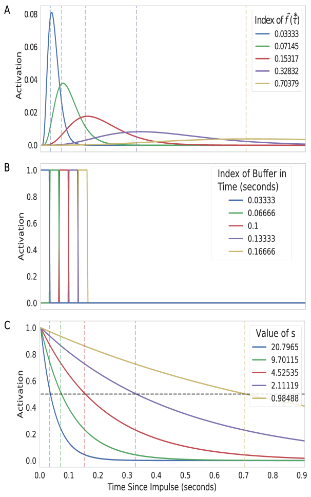
Our goal is to provide a memory representation that tackles both difficulties. Below, we describe and characterize this model, called the Scale-Invariant Temporal History (SITH). Then, we consider the implications of utilizing SITH in place of either a FIFO buffer of size $N$ or a family of exponentially decaying representations, all of which are illustrated in Figure 1. The capabilities of each representation are compared through manipulations of two reward-driven, arcade-style games. Finally, we compare the performance of all three representations, and discuss how SITH can enrich memory systems in AI.

Figure 1: SITH efficiently extends into the past, unlike a buffer, and retains temporal order information more clearly than exponential decay. For all visuals presented here, a single impulse was presented for 0.0033 seconds, followed by a decay of 0.9 seconds; the activation values of each index for each representation are shown through time. (A) Activation of SITH through time. By choosing five evenly spaced indices from the full output of SITH, we retrieve a sparse, compressed representation of a single feature following its transient activation; each line represents an index in this subset, which is a temporal receptive field centered on the corresponding dashed, vertical line. Note the logarithmic spacing of centers, as well as the asymmetric, increased spread of activation of fields centered further in time. (B) Activation of a FIFO buffer through time. A buffer of size 5 has perfectly accurate storage of the impulse, but does not span long distances in time. Here, each buffer index stores one frame of game input, equivalent to $1/30^{\text{t}h}$ of a second. (C) Activation of exponentially-decaying representations through time. Each line denotes the activation of a different decay rate through time. The decay rates $s$ were chosen to have an activation at 0.5 at the matching temporal receptive fields in SITH. While the exponential decay does span a large amount of time, there is little information indicating when the impulse occurred, just that it happened at some point.

2 Scale-Invariant Temporal History: An efficient representation for learning across scales

SITH builds on a body of work in neural computation and cognitive psychology, as found in K. H. Shankar & Howard (2013) and Howard, Shankar, Aue, & Criss (2015), along with neurological evidence for its existence in mammalian brains detailed in M. W. Howard et al. (2014) and Z. Tiganj, Cromer, Roy, Miller, & Howard (2018). The method results in a logarithmically compressed representation that coarse-grains the history of what happened, and when. With this logarithmic compression, the number of nodes necessary to represent a time $\tau$ in the past goes up only like $\log\tau$: an exponential savings. The cost is that the resolution at which past events can be discriminated goes down linearly with the distance into the past. This decrement in accuracy obeys the Weber-Fechner law, a fundamental result in human and animal psychophysics (Fechner, Howes, & Boring, 1966). Furthermore, this form of coarse-graining can be shown to be an optimal solution to processing signals with a particular scale, but where the agent uses an uninformative prior for the unknown scale (Howard & Shankar, 2018).

2.1 Model Definition

For each feature in an agent’s observation, one can imagine a set of units that have temporal receptive fields. The units that fire when a feature was active closest to the present have smaller receptive fields that are centered closer together, much like the fovea of the retina (Van Essen, Newsome, & Maunsell, 1984). These units provide high temporal accuracy, but are activated for only a small time into the past. Conversely, neurons that are active further away from the present have larger receptive fields that are spaced further apart. In keeping with prior work (K. H. Shankar & Howard, 2013), the nodes of this representation are evenly spaced on a logarithmic scale.

To attain this SITH representation from a stream of input, we first compute a set of leaky integrators

$$\frac{dF(s)}{dt}=-sF(s)+f(t),$$

where each unit is indexed by its value of $s$ and driven by the function $f(t)$ that describes the activation of a particular feature (in our case pixels on a screen). It can be shown that this set of leaky integrators implements the Laplace transform of the input function over past times $f(\tau<t)$. We approximate the inversion of the Laplace transform using a linear operator $\mathbf{L}^{-1}_{k}$ that provides a discrete approximation to the Post inversion formula (K. H. Shankar & Howard, 2013).

The goal of this method is to approximate the history of the input function leading up to the present $f(\tau<t)$. We make this estimate by approximating the inversion of the Laplace transform of this history. For each unit in $F(s)$, we assign a new unit in $\tilde{f}(\overset{*}{\tau})$, where $s$ and $\overset{*}{\tau}$ are in one-to-one correspondence as $s=-k/\overset{*}{\tau}$. At each moment we compute

$$\tilde{f}(\overset{*}{\tau})=\mathbf{L}^{-1}_{k}F(s).$$

The integer $k$ controls the degree of approximation. The error in the inversion introduces a coarse-graining function that depends on the value of $k$ (for these simulations $k=4$.) As $k\rightarrow\infty$ the inversion becomes perfect. If we refer to the present as $t=0$, a node with a particular value of $\overset{*}{\tau}$ provides a coarse-grained estimate of the true function, $\overset{*}{\tau}$ in the past: $\tilde{f}(\overset{*}{\tau})\simeq f(\overset{*}{\tau})$, with equality as $k\rightarrow\infty$. However, the coarse-graining is scale-invariant; the error in the reconstruction can be shown to be proportional to $\overset{*}{\tau}$. By choosing $s$ such that the $\overset{*}{\tau}$ values are logarithmically-compressed, we construct a scale-invariant temporal history. One approach to parameterizing $s$ (and, consequently, $\overset{*}{\tau}$) is

$$s_{i}=-k/\overset{*}{\tau}_{i}=\overset{*}{\tau}_{0}(1+c)^{i},$$

where $0\leq i\leq N_{\overset{*}{\tau}}-1$, and $N_{\overset{*}{\tau}}\geq 2k+1$. This definition is used in both these simulations, and previous work (K. H. Shankar & Howard, 2013). Due to the one-to-one correspondence between $s$ and $\overset{*}{\tau}$, note that $\lvert s\rvert=\lvert\overset{*}{\tau}\rvert=N_{\overset{*}{\tau}}$. Note that the representation at a particular value of $\overset{*}{\tau}$ is independent of other values of $\overset{*}{\tau}$.

The evolution of the representation depends only on the values of $F(s)$ in the neighborhood of $-k/\overset{*}{\tau}$. This means that although the representation can be thought of as continuous, we can sample whatever discrete values we find convenient for a particular application. In the applications described here, we take only four or five (dependent on the environment) discrete values and use it in place of traditional FIFO buffers and sets of exponentially decaying features. A comparison of these representations is illustrated in Figure 1.

2.2 Parameter Characterization

SITH is governed by relatively few parameters, though each can have subtle effects on the resulting representation. As discussed above, $N_{\overset{*}{\tau}}$ sets the size of the ensemble in $F(s)$. Additionally, there are three other parameters that determine the temporal scale, spacing, and fidelity of each value in $\tilde{f}(\overset{*}{\tau})$, which are $\overset{*}{\tau}_{0}$, $c$, and $k$.

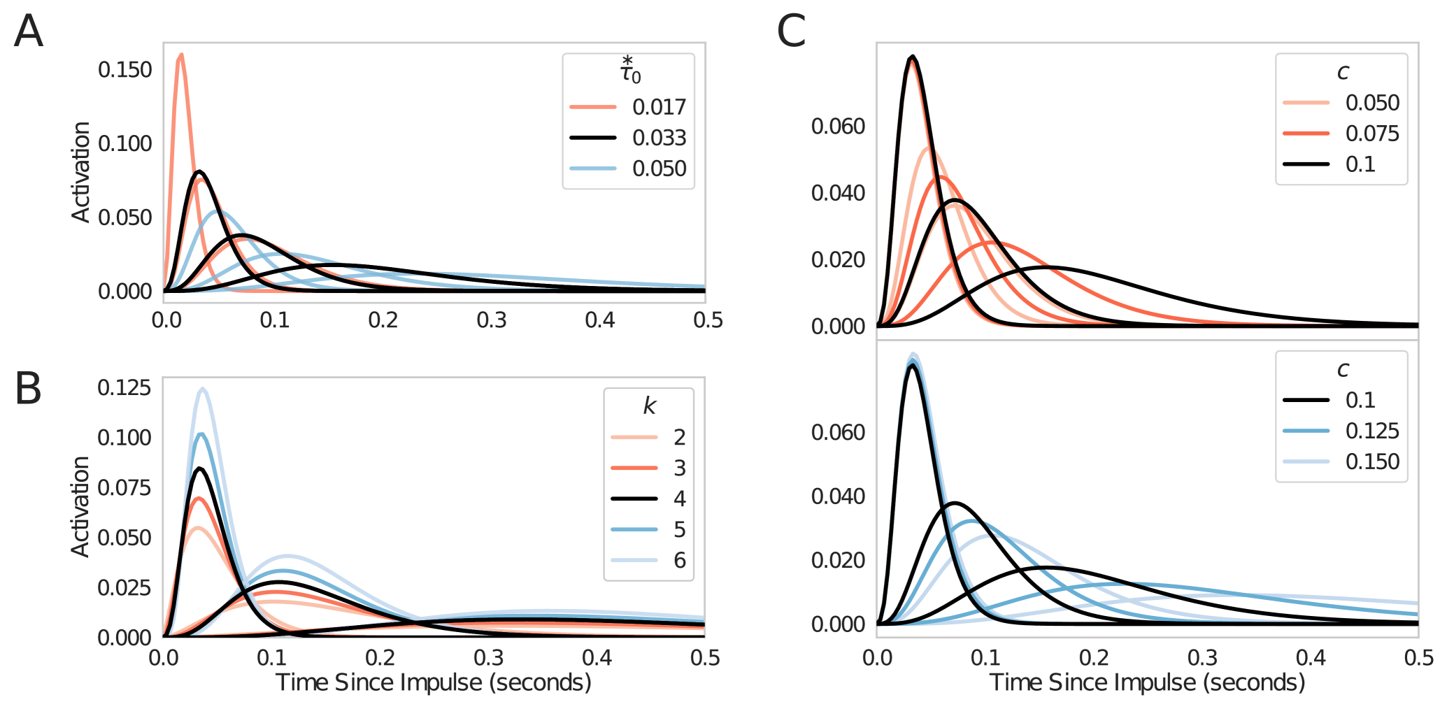
As given in our approach to constructing $s$, $\overset{*}{\tau}_{0}$ acts as the value of the first $\overset{*}{\tau}$ found in $\tilde{f}(\overset{*}{\tau})$. This can also be seen as the selection of the timescale captured in the first index of $\tilde{f}(\overset{*}{\tau})$, with logarithmically increasing scales in subsequent indices. This is visualized as a linear “shift” in the peaks of each index in $\tilde{f}(\overset{*}{\tau})$, with an accompanying spreading of activation; this is shown in Figure 2A. For these simulations, we chose $\overset{*}{\tau}_{0}$ to be equal to one timestep in our discrete time series, and we recommend this approach for all discrete time series data.

The parameter $c$, which controls the spacing of the $s$ values, also results in a “shift” of activation peaks, but a shift that is logarithmically increasing. With all other parameters fixed, this causes a relatively small change in the early $\tilde{f}(\overset{*}{\tau})$ indices, but can drastically change the spread of activation later in the ensemble. Practically speaking, $c$ can be tuned to maximize SITH’s temporal spread, while balancing the desired information redundancy. The effect of modulating $c$ is illustrated in Figure 2C. In these simulations, we set $c=0.1$, which we recommend for general usage.

Finally, the positive integer $k$ determines the degree of approximation in the Post approximation of the inverse Laplace transform, $\mathbf{L}^{-1}_{k}$. For any feature in some $\overset{*}{\tau}_{i}$, increasing $k$ increases the number of surrounding $\overset{*}{\tau}$’s that are used in the linear combination to calculate $\tilde{f}(\overset{*}{\tau}_{i})$. Values of $k$ are directly proportional to SITH’s accuracy in recreating past events, at the cost of increasing the number of calculations performed and the required number of $s$ values. Increasing $k$ causes the peaks in each index of $\tilde{f}(\overset{*}{\tau})$ to become sharper, and more defined, as the approximation becomes more accurate; this is illustrated in Figure 2B. Here, as in other works, we have $k=4$, and we recommend this as a general default value.

Figure 2: Three parameters control SITH’s minimum scale, fidelity, and spacing. For all figures, an impulse with activation 1 was presented for 0.033 seconds, followed by a delay of 0.5 seconds. Unless otherwise indicated, all parameters are equivalent to those used in the first set of simulations; the black line in each plot corresponds to the value used in these same simulations. After indexing linearly into $\tilde{f}(\overset{*}{\tau})$, only the first 3 values are shown for clarity. (A) Modulation of $\overset{*}{\tau}$ scaling. This parameter sets the value of the first index in $\overset{*}{\tau}$, and constantly scales subsequent values. This can be seen in the constant shift of activation peaks left and right, for smaller and larger values, respectively, of $\overset{*}{\tau}$. (B) Modulation of degree of approximation $k$. By increasing $k$, more values from $F(s)$ are integrated in the $\mathbf{L}^{-1}_{k}$ operator, creating a more precise approximation of $f(\overset{*}{\tau})$. This produces stronger peaks in activation, at the cost of an increase in number of operations performed and required size of $s$. (C) Modulation of $c$ spacing. Parameter $c$ determines the spacing of the $s$ values. As shown here, changes in $c$ result in a logarithmic “shift” in the peak activations. This nonlinear shift increases logarithmically, unlike the constant shift from modifying $\overset{*}{\tau}$. For clarity, the plot is divided with descending values in the upper panel and ascending values in the lower.

3 Testing Environments

To test the demands of maintaining information over a range of timescales on a learning agent, we required a task that is solvable by human agents, presents stimuli through time, and has a meaningful reward structure. As demonstrated in Mnih et al. (2015), video games meet all of these criteria.

3.1 Catch: A simple application to evaluate the ability to learn and express temporal relationships.

To reduce complexity and focus on the properties of the various representations of interest, we first tested our agents in a noise-free, simple video game environment that would not require convolution layers to extract meaningful features. Catch, modified slightly from previously published versions, provided a simple testbed to illustrate the essential advantages of a scale-invariant representation (Ba et al., 2016).

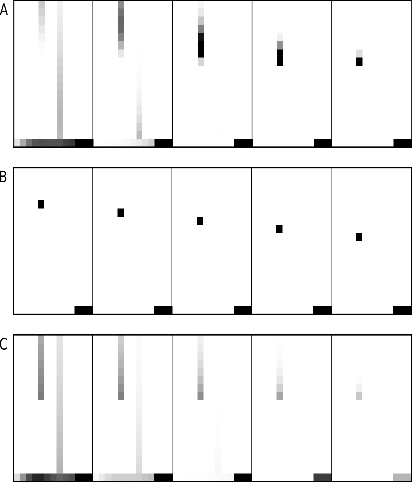
In Catch, an agent moves a basket left and right at the bottom of the game screen in order to catch falling balls that start at the top of the screen. Our instantiation of Catch is a game board comprising an $18\times 13$ matrix of binary pixels; here, 1 represents the presence of a game piece, and 0 represents the absence of any game pieces. At the bottom of the game board is a $1\times 3$ basket. Balls are spawned at the top of the game board, with only one ball on the board at a time, and start to move down vertically to the bottom at a constant rate of one pixel each frame. This is visualized most clearly in Figure 4B. The agent receives a 1 point reward if the ball overlaps with the basket when the ball reaches the bottom row. If the ball does not overlap, then the agent receives a -1 point punishment. During every frame, the agent has to make a decision to either move the basket one pixel to the left, one pixel to the right, or to not move at all. For most of the tests, the game ends after 10 balls fall to the bottom row, regardless of whether they were caught; as explained below, we also performed limited testing with a variant of Catch with only 1 ball per game, with otherwise identical task parameters. New balls are spawned after the previous ball reaches the bottom of the screen, so there is only a maximum of 1 ball on the game screen at all times during training and testing. With the consideration that the basket is 3 pixels wide, the screen is 13 pixels wide, and there are 10 balls for each game, it is important to note that chance performance for an agent performing random movements is approximately $-5$.

A simple modification to this game was made to demonstrate the effects of obscuring parts of the stimuli, similar to the partially observable version of Catch found in Ba et al. (2016). This variant, which we call Hidden Catch, retained all properties of Catch as described above, with one exception. In the game screen, a mask of varying size was placed over all pixels in a set amount of rows, starting from the second to bottom-most row. This mask set these pixels’ values to 0, removing all information for the agent. The agent was able to see and move the basket in the same manner as before, however, the ball disappeared after passing behind the mask. The agent received no further information about the ball until the reward or penalty was given. In theory, so long as the agent can store information about the horizontal position of the ball, an optimal score can be attained. However, by increasing the size of the mask, the agent must have the necessary memory representation to learn this association and attain robust performance. This leads to the fundamental computational challenge posed by Hidden Catch, namely that the model must bridge larger and larger temporal gaps in order to behave optimally.

3.2 Flappy Bird: A more complex time-dependent environment

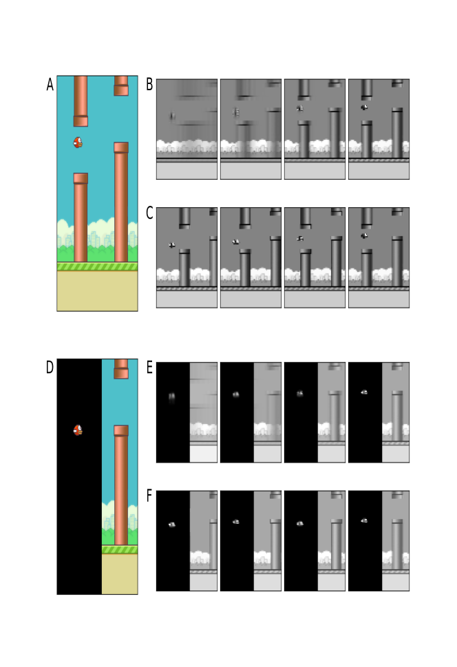
After detailing the behavior of SITH in a simple, noise-free environment, we sought to test in a higher-dimensional, noisier setting to demonstrate that SITH can be combined with other standard deep-learning approaches, namely convolutional layers. Our chosen game was an emulated version of the game Flappy Bird (Tasfi, 2016). In Flappy Bird, the goal of the agent is to navigate its character avatar between pipes while constantly being pushed rightward. The agent can either “flap”, leading to a gain in upward momentum, or perform a “do-nothing” operation, letting gravity pull the avatar down. Once the avatar makes it through the gap in the pipes, the agent receives a reward of 1. If the avatar touches the ground, the top of the screen, or the pipes, the game is over, and the agent receives a penalty of -5. The game is functionally endless, so an optimal agent would seek to go between as many pipes as possible, for as long as possible. As seen in Figure 6A, this environment has many more features than Catch (7,056 features valued between 0 and 1, as opposed to 234 binary features, in these experiments). Critically, Flappy Bird also contains irrelevant features that simply add noise to the reward prediction (i.e. background details, like bushes).

Similar to Hidden Catch, we also transformed Flappy Bird into a partially-observable task with state correlations through time, by masking pixels. This variant of Flappy Bird removes information of all features behind and in front of the agent avatar. Critically, this mask hides the location of the pipes at the time of reward or punishment. The agent is only able to see the position of the avatar, and the normal environment details beyond a certain point from the avatar. Thus, as illustrated in Figure 6D, the agent must retain a memory of where the pipes were, as well as how long ago they last saw them, in order to flap at the correct time to dodge them.

4 Models Tested

4.1 Models for Playing Catch

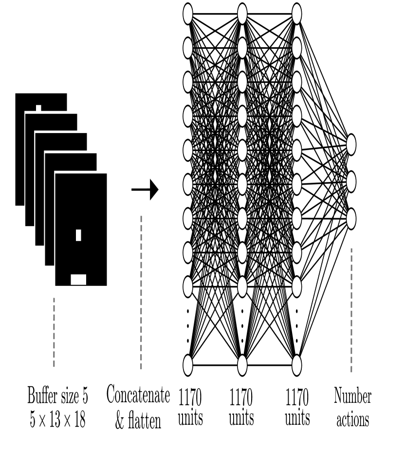
As shown in Mnih et al. (2015), Deep Q-learning Networks (DQN) are extraordinarily adept at solving simple video game environments. In order to provide the DQN with some sense of temporal change, previous applications have used a FIFO buffer of experience as input to the network. The FIFO buffer keeps a perfectly accurate history of the past $N$ game frames. For Catch specifically, a visualization of a buffer of size 5 during a moment of gameplay is shown in Figure 4B. The contents of the buffer are concatenated, flattened, and passed into the network via the input layer. Thus, the input to the network is of size $N\times S$, where $S$ is the size of the stimulus set (game screen) at a single time point. During our simulations in Catch, each game screen was $13\times 18$ pixels. We tested the performance of a buffer of sizes 1, 5, and 10, resulting in inputs of sizes 234, 1170, and 2340 features, respectively. We tested these representations on a fully visible version of Catch, as well as versions of Hidden Catch with logarithmically-spaced mask sizes of 1, 2, 4, 8, and 16.

Besides a buffer, another approach taken in the RL literature is the use of exponentially-decaying sets of features, such as in Doya (2000). Indeed, this approach is similar to the first process performed in SITH, the calculation of the Laplace transform of the input. To capture some given timespan, the decay rate is lowered between subsequent feature sets, maintaining activations from stimuli further back in the past. We found it informative to test the performance of an exponentially-decaying representation, for two reasons: 1) as an analog for the models described in previous work, and 2) as a justification for the second process in the SITH model, the inverse Laplace transform from exponentially-decaying representations into a logarithmically-compressed representation of what features were active when in the past. Recalling the parameters that compose SITH, we chose values of the decay rate $s$ that would reach half of their initial activation values at the time of each $\overset{*}{\tau}$ used in our instantiation of SITH; the nature of these decaying features is shown in Figure 1C. This resulted in $s=[20.7965,9.70115,4.52535,2.11119,0.98488]$. The 5 decayed feature representations are analogous to that of 5 stored experiences in a buffer, with the additional time-spanning nature of exponential decay. This representation is concatenated, flattened, and passed to the agent. The resulting exponentially-decaying feature set is illustrated in Figure 4C. We tested agents given this representation on Catch with logarithmically spaced mask sizes of 0, 1, 2, 4, 8, and 16. As we will explain below, understanding the results of these tests was aided by testing on a slightly modified environment. These similar tests, with agents given this same exponentially-decayed feature representation, were tested on Catch with only 1 ball per game; the environment shape and mask sizes were kept to be the same as previous tests.

Finally, we also trained and tested an agent using our SITH representation with five nodes per feature. An illustration of the input layer during a moment of gameplay with a SITH representation of 5 nodes is shown in Figure 4A. Note the “smearing” of the temporal representation and also how the nodes span logarithmic (as opposed to linear) distances into the past. Each agent was then tested on versions of Hidden Catch with logarithmically-spaced mask sizes of 0, 1, 2, 4, 8, and 16.

During our simulations with Catch, we used simple densely-connected feedforward networks, where the number of parameters depended on the number of indices $N$ used in the representation model. All networks trained on the Catch game contained 4 layers: an input layer of size $S\times N$, two hidden layers of the same size as the input layer, and an output layer of size 3, to indicate all possible movements of the basket (left, right, and no-op). An illustration of the model with a FIFO buffer of size 5 is shown in Figure 3.

Figure 3: Fully connected DQN with representation outside the network allows for comparisons between working memory input representations. The most recent frame from the catch game is input into a FIFO buffer. Then we concatenate the frames and flatten into a $1\times 1170$ ($5\times 18\times 13$) vector. That vector is the input to our DQN, which consists of 2 fully connected hidden layers, same size as the input vector, and outputs a $1\times 3$ vector where the max of those 3 numbers indicates the action our agent should take that frame.

All densely-connected networks learned to approximate the Q function in a Q-Learning RL paradigm, with a discount rate of 0.9. The memory store for experiencing replay retained up to 50 previous full games, with each game consisting of 10 balls worth of frames. For each frame observed from the environment, the network went through one session of experiencing replay, which consisted of replaying 10 random full games from its memory store. These networks were trained using the Adagrad optimizer with a learning rate of 0.01, an epsilon of $1\times 10e^{-8}$, and decay of 0 (Chollet, 2015/2015). Networks were trained and tested on 500 epochs, where an epoch consisted of the back-propagation of error from a session of experiencing replay. Networks were tested on 100 games every 5 epochs of training, and tested on 1000 games after completing training. These models were trained and tested during five independent learning runs to quantify variability in learning performance. We note here that for our tests on Catch with with one ball per game, each game was $1/10^{\text{t}h}$ the length of other tests with Catch. For a more even comparison to other results, the replay buffer was increased to a size of 500 games, and each network was tested for 5000 epochs. This ensured that each network was able to replay experiences similar distances into the past, and was trained on a similar number of frames.

Figure 4: SITH produces an extended, but focused, recreation of events in pixel space compared to a buffer and exponential decay. Visualization of all representations tested with Catch, at the same point in the same game. The most recent input is represented in the rightmost index, and each representation spans further back in time going leftwards. Colors are inverted and normalized within representation, for clarity, such that darker values show stronger activations. (A) Visualization of SITH given states of Catch. SITH spans logarithmically increasing points into the past, while maintaining information of when a feature was active. This can be seen by the shift in intensity of the ball pixels, which follows the past, true path of the ball. (B) Visualization of a buffer given states of Catch. While information is perfectly preserved, that information can only span a short discrete interval into the past depending on the length of the buffer. (C) Visualization of exponential decay given states of Catch. While the representation shown here spans further back than SITH, it is unclear when each feature was active in the past. This can be seen by the most recent position of the ball having the highest activation (in regards to pixels outside of the basket) in all indices. This does not provide as useful a recreation of past experience, only the knowledge that a feature was active at some point in the past relying on tiny relative changes in activation to estimate when it might have occurred.

When testing the models that received either SITH or exponentially decaying representations as the input, we had to make some assumptions with regard to real-world timing. The first was to treat each Catch game frame as if $1/30$ seconds passed. This assumption allowed these representations to update their array of decaying cells in a real unit of time. Specifically, each frame of Catch was presented for $1/300^{\text{t}h}$ of a second and decayed for $1/30-1/300$ seconds.

For the SITH model, due to the overlap in the receptive fields, there was no need to pass in the the entirety of $\tilde{f}(\overset{*}{\tau})$, for every feature, into the neural network. Instead, we “sliced” into SITH at logarithmically-spaced points into the past. Here, the set of all temporal receptive fields were centered around $\overset{*}{\tau}=[0.03333333,0.07145296,0.15316577,0.32832442,0.70379256]$, which are in units of seconds. The size and shape of these receptive fields are shown in Figure 1A. In effect, SITH acts as a “blurred” representation of the past, where each “slice” into the past was a temporally-blurred game screen of features, each containing varying amounts of activation and temporal specificity.

Similar to the buffer, both the exponentially decayed and SITH representations were concatenated and flattened before acting as input to the network. The 5 time indices pulled from SITH gave rise to network parameters equal in size to that of the model with a buffer size of 5; i.e., 1170 input features. This was also the case with the 5 exponentially decayed feature sets. Networks that are given either an exponentially decayed representation or SITH follow the exact configuration as in Figure 3, but with a corresponding input representation in place of a FIFO buffer.

4.2 Models for Playing Flappy Bird

Figure 5: A standard DQN architecture with convolutional layers allows comparisons between buffer and SITH representations in more-complex games. Game frames are preprocessed in a manner described in the main text, and illustrated in Figure 6B, C, E, and F. The various representations are processed through 3 convolutional layers, then passed through one fully connected hidden layer, to the output layer. In Flappy Bird, the number of actions $M=2$. Each output unit predicts the future reward for a given action, and the maximum rewarded action is chosen for the agent to perform. Only a buffer representation is illustrated here, but a SITH representation utilizes the same network design and frame preprocessing.

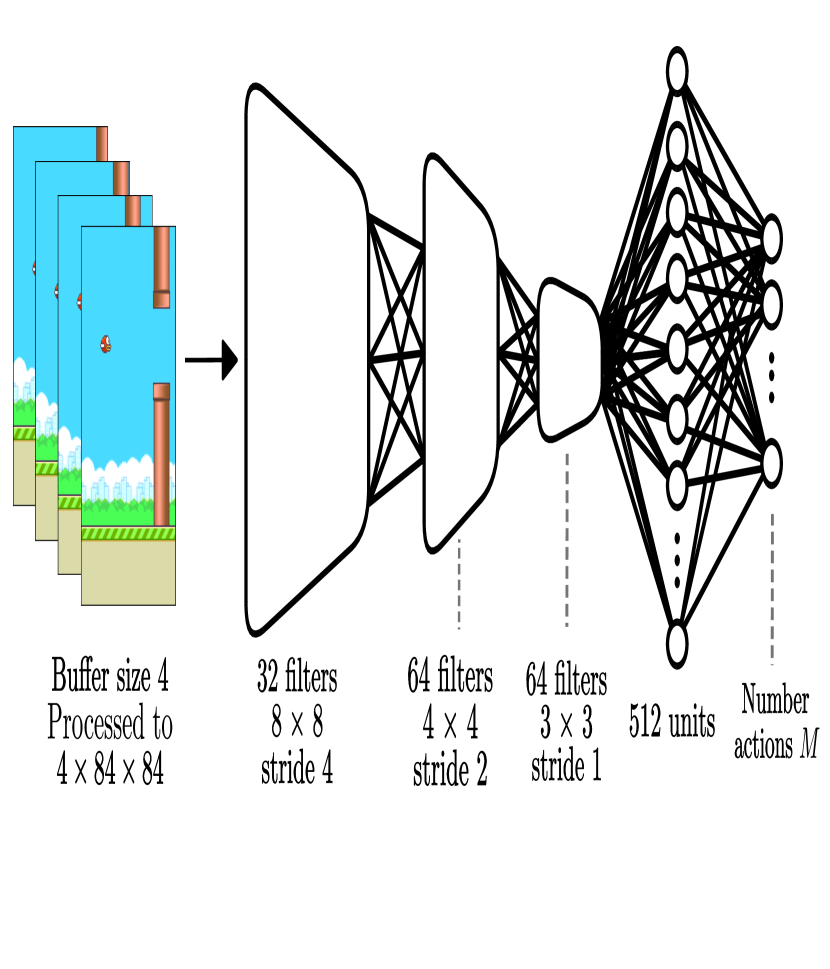
After testing our models in the game Catch, we sought to test SITH in a noisier, more compelling environment, requiring a more specialized network architecture to learn the task. For this comparison, we measured the performance of a buffer of size 4 against a SITH representation with 4 “slices” into the past. Here, SITH is indexed at $\overset{*}{\tau}=[0.03333334,0.08645808,0.22425,0.58164674]$. As we did with the game Catch, we set the length of one frame to be $1/30^{\text{t}h}$ of a second; the input screen was presented for $1/300^{\text{t}h}$ of a second, followed by a delay of $1/30-1/300$ seconds.

Taking after Mnih et al. (2015), we utilized a convolutional neural network (CNN), illustrated in Figure 5, with the same structure (Jo, 2017/2017). In the preprocessing step, the representations are converted to grayscale, then down-sampled and trimmed to a size of $84\times 84$ pixels. This $4\times 84\times 84$ array of feature sets is then given to the network as input. An illustration of this step is shown for a buffer in Figure 6C and for SITH in Figure 6B. The same preprocessing was performed on the partially obscured variant of Flappy Bird, as seen in Figure 6E and F.

The network was trained with the Adam optimization algorithm, with a learning rate of 0.0001, and a smooth L1 loss function to calculate error (Paszke, 2016/2017). Training occurred over 1,000,000 epochs, where each epoch was one frame of Flappy Bird. Training was performed in 5 independent runs for each representation (buffer and SITH), and for each game variant (fully visible and partially obscured Flappy Bird), resulting in 4 interactions being tested. During each epoch, a random minibatch of 32 previous $(s_{t},a,s_{t+1},r)$ (state, action, next state, reward) tuples was pulled from the experience replay buffer, which itself had a maximum size of 50,000 tuples. This minibatch was used to backpropagate errors through the network, with one minibatch for every epoch. By the means of a DQN, this network approximated the Q-function found in Q Learning, with the discount factor $\gamma=0.99$. An $\epsilon$-greedy policy was utilized to balance exploration and exploitation, where $\epsilon$ started at 1.0, and was exponentially reduced to 0.1 according to $\epsilon_{i}=\epsilon_{i-1}e^{\frac{\text{epoch}_{i}}{\text{decay}}}$, with a decay of 100,000. Similar to Mnih et al. (2015), a target network had its weights periodically copied from the network being trained, and was used to calculate $Q(s_{t+1},a_{t+1})$ when determining loss. This target network was updated every 1000 epochs, and increased training stability in the “true” network. During training, one test game of flappy bird was played every 900 epochs, giving a view of how the network performed while training.

Figure 6: SITH maintains rewarding information in a more complex game. (A) Illustration of a single screen of the visible variant of Flappy Bird. The original screen size is $288\times 512$ pixels. (B) Output of the SITH representation when given grayscaled and down-sampled input. The most recent experience is maintained in the rightmost cell, and spans further back into the past going left. (C) Output of a buffer representation when given grayscaled and down-sampled input. The most recent experience is in the rightmost cell, and experiences reach further into the past going left. (D) Illustration of the partially obscured variant of Flappy Bird, at the time of reward. The bird avatar needs to remain visible, otherwise the task becomes impossible. (E) Output of SITH representation given grayscaled and down-sampled input in partially obscured Flappy Bird, at the time of reward. Note how the item that leads to reward and punishment, the pipes, remains visible in the cell spanning the most amount of time. (F) Output of the buffer representation, given grayscaled and down-sampled input. Note how the most important features pertaining to reward, the pipes nearest to the avatar, are completely obscured at the time of reward.

5 Results

5.1 Performance in Catch

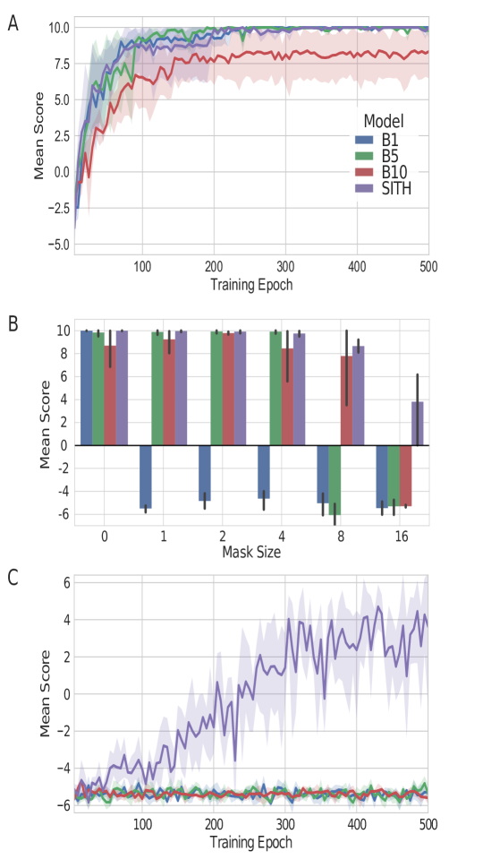
Agents given either a buffer or SITH as representations were trained on the fully visible catch game. As illustrated in Figure 7A, these models all performed well; over 1000 testing games, they received an average score at or close to 10, the maximum score possible. Despite having more information about the environment than a FIFO buffer of 1, the models based on FIFO buffers of size 5 and 10 had some variance in their final performance. This was most likely due to the corresponding networks having many parameters with extraneous information leading to overfitting. Overall, high performance was to be expected and served to establish a baseline for the critical test offered by Hidden Catch.

After establishing baseline functionality by training and testing on the fully visible game of Catch, we then trained and tested agents with these representation configurations on Hidden Catch. These trials were run using logarithmically-spaced mask sizes, as seen in Figure 7B. This illustration demonstrates the inflexible nature of the FIFO buffer. Each network performed well above chance as long as its FIFO buffer was able to capture the ball before being hidden behind the mask. However, as soon as the mask obfuscated that information from the network’s history, the network failed. This is because the models that use FIFO buffers are not able to bridge temporal gaps larger than the size of the FIFO buffer. The ball is hidden from the network during the most critical observations. For example, the FIFO buffer of 1 could only present the most recent observation to the network, but performed optimally in a fully visible environment. A similar result occurs when testing the FIFO buffer of size 5 with a mask of 8, and a FIFO buffer of size 10 on a mask of 16.

We note the success of the model that took a SITH buffer as input at a wide range of time scales, also seen in Figure 7B. The agent learned to play all versions of Hidden Catch with scores well above chance due to the logarithmic spacing and preservation of time. Even in the most difficult scenario, where all but two rows were hidden from the network, the SITH model performed well above chance, as seen in Figure 7C. Thus, the network is able to create a mapping of the ball’s location with that of a reward. As is the nature of SITH, however, this lossy representation is also responsible for slower learning during training with increasing mask sizes, as well as higher variance in the final scoring benchmark; this is visualized and most clearly evident for the mask sizes of 8 and 16 in Figure 7B.

Figure 7: Buffers fail when the ball cannot be seen at reward time while SITH performs the same or better than a buffer for all mask sizes. (A) Performance of SITH and buffers in fully visible Catch. With no obfuscation, both SITH and a FIFO buffer are sufficient for learning Catch. This learning occurs at a similar rate, given the same network architecture and training parameters. Shaded regions indicate 90% confidence interval over 5 independent simulations for each model, with each model tested on 100 games at each point. (B) Trained performance of each model over mask sizes. As the size of the mask (i.e. amount of feature obfuscation) increases, buffers fail when rewarding information is outside the buffer size. Meanwhile, SITH is able to match buffer performance in lower mask sizes, while maintaining rewarding information over longer timescales. This leads to performance well above chance in all configurations. Plotted here is mean performance on 1000 games for each model after training, with 5 independent simulations per model and per mask size. Black lines indicate the 95% confidence interval about the mean. (C) Performance of SITH and buffers in fully obscured Catch. On a mask size of 16 (the max amount of obfuscation with this configuration) buffers of sizes 1, 5, and 10 all fail to learn even the relatively simple Catch game. SITH is sufficient for performance well above chance, due to its farther-reaching temporal span. Shaded regions indicate 90% confidence interval over 5 independent simulations for each model, with every model tested on 100 games at each point.

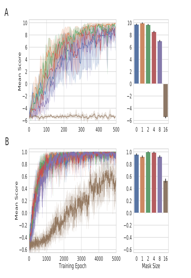
To further understand the potential advantages of SITH, we also tested agents with an array of exponentially decaying feature sets on Catch and Hidden Catch. The structure of this representation is illustrated in Figure 4C. As expected, this model performed nearly optimally in the visible variant of this game, as seen in Figure 8A. However, it performed no better than chance when tested on Hidden Catch with a mask size of 16. This is in contrast to the performance of SITH on the same game, which performed well.

Due to the selected values of $s$, this representation spanned further back into the past than did the SITH representation. This suggests that when representing the past, more is needed than simply spanning longer durations. Supporting this hypothesis demanded further testing with exponentially-decaying sets of features. To simplify the task, the state space of the exponentially-decaying set had to be reduced. This was achieved by providing only 1 ball for every game of Catch, causing a reset of the representation after each ball hit the ground. By not maintaining irrelevant information on previous balls, the number of possible values of the representation decreased. Testing was again performed on logarithmically-increasing mask sizes, and results are shown in Figure 8B. While the agent took significantly more epochs to learn the reward structure with a mask of 16, the representation is clearly capable of capturing long-term dependencies, otherwise the agent would never perform above chance.

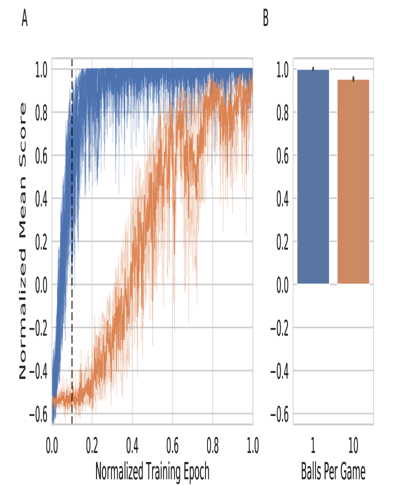
Knowing this capability, agents with exponentially-decaying sets were trained on games with a mask of 16, and either 1 or 10 balls per game, and were trained an order of magnitude more epochs. Results of this more focused testing are shown in Figure 9. Here, it is shown that the reward structure of both game configurations can be learned, given enough training epochs. We note that the exponentially decaying set required a fivefold increase in epochs to match the performance of SITH on the same task (as seen in Figure 7C), and a tenfold increase to achieve near optimality.

Figure 8: Exponentially decayed sets do not clearly encode past events. All shaded regions and bar extensions indicate 95% confidence intervals. (A) Performance of exponential decay on Catch with 10 balls per game. Performance as a function of training epoch is shown, with 5 independent simulations run for every game configuration. The representation has the necessary temporal reach for all levels of obfuscation. However, with 10 balls in every game, noise from previous balls hampers learning, especially with high obfuscation. Also plotted is the final performance for each game type, after training on 1000 games. (B) Performance of exponential decay with 1 ball per game. Performance is shown during training, for 5 independent simulations per game configuration. By reducing the number of balls per game, no noise is carried over from previous balls. The representation has sufficient temporal span, and becomes more separable with the reduced noise. Final performance of each simulation and game configuration, over 1000 games, is plotted on the right.

Figure 9: Exponentially-decayed sets require five times more training than SITH on the same Catch parameters. With exponentially-decaying feature sets, networks are able to achieve near optimality given longer training times. Scales are normalized for clarity of comparison. In order to equate the total amount of training, networks trained with 1 ball per game were trained for 50000 epochs, with chance performance at -0.5 and possible mean scores between -1 and 1, inclusive; networks trained with 10 balls per game were trained for 5000 epochs, with chance performance at -5 and possible mean scores between -10 and 10, inclusive. (A) Performance of networks during training. Each line corresponds to network performance while being trained on games with different numbers of balls per game; the dashed vertical line indicates where training was stopped in previous tests. Shaded regions indicate 95% confidence intervals. The number of balls per game has a significant effect on performance, though the information needed for optimal performance is still present in the exponentially-decaying set. Nevertheless, agents with the exponentially-decayed representation required 5 times as many epochs to match the performance of agents with SITH, as seen in Figure 7C. (B) Testing performance of networks trained on each game after training; error bars indicate 95% confidence interval. Despite the slower rates of learning, networks with exponentially-decaying sets tested in both environments were capable of achieving near optimality.

5.2 Performance in Flappy Bird

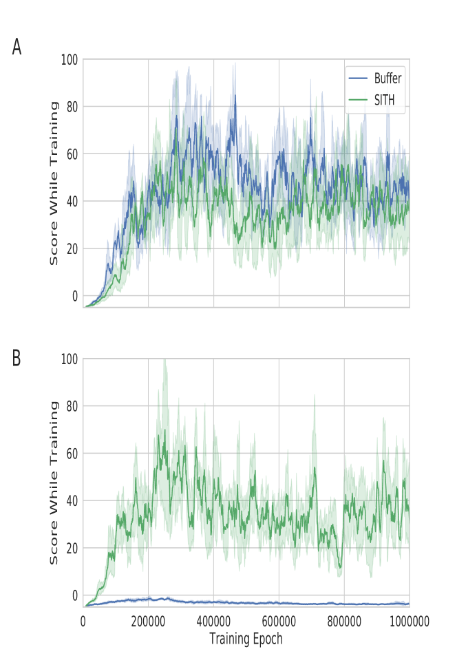
After demonstrating the advantage of SITH over other models, we wanted to measure performance of SITH in a more “real-world” setting, requiring more complicated neural network models to attain high levels of performance. As outlined above, we selected a variant of the game Flappy Bird, which requires training a convolutional neural network to solve it. Our first simulation was to establish baseline performance and verify that both the buffer and SITH models could learn to play a fully visible variant of Flappy Bird. As shown in Figure 10A, the performance of both models is comparable, with overlapping 95% confidence intervals over the independent training and testing runs.

When testing in the partially observable variant of Flappy Bird, results are consistent with those in the Catch game. As seen in Figure 10B, a SITH representation allows the network to achieve scores similar to those of the fully visible simulations. For the buffer representation, however, there is no discernable pattern of learning and the network rarely performs above chance. These results demonstrate that SITH can be used as input to a convolutional neural network. This network can then extract meaningful spatio-temporal representations that can help solve partially-observable complex environments which require representations of the past to guide actions in the present.

Figure 10: SITH performance matches or exceeds a buffer, even with a CNN required to learn a more-complex game. All shaded areas indicate 95% confidence intervals about the mean. For clarity, all plots are shown with a rolling mean with a window size over 10 epochs. (A) Performance on regular version of Flappy Bird. Without any obfuscation, both the FIFO buffer and SITH are capable representations for learning Flappy Bird. Shown here are 5 independent simulations for each model. (B) Performance on partially obscured Flappy Bird. By obscuring pipes in game, the buffer is unable to maintain information for rewarding features. On the other hand, SITH is able to maintain this information, even when passed to a convolutional layer. Shown are 5 independent simulations for each model.

6 Discussion

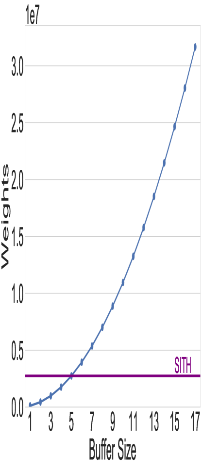
We presented a novel approach for representing the history of features in a scale-free, optimally fuzzy, and neurally-plausible manner. We tested a DQN using a SITH representation as input for a toy example of the game Catch, and its variant, Hidden Catch. We verified that the model, given SITH as input, performs well when features are fully visible, and, more importantly, when features are partially observable. Additionally, we showed that this performance in Hidden Catch only needs the same number of model parameters as a model based on a FIFO buffer of size 5 (Figure 11) and still outperforms models with a FIFO buffer of size 10 across a wider range of mask sizes. Moreover, we determined that a FIFO buffer of size 17 would be needed to perform well in a game of fully hidden catch at the cost of many more resources than a SITH representation with 5 nodes. We also tested a set of exponentially decaying features in the same environment and found it required many times the number of training epochs for a highly obscured task. This test suggests that temporal reach is not the only important feature of a representation, but also clarity and information of what happened when.

Finally, we also tested our model in a more complex, noisy environment, using more specialized CNNs. As it was in a simple environment, SITH was a capable representation in both fully visible and partially observable environments, while a FIFO buffer failed in the partially observable variant. The successful utilization of CNNs, and its ability to track visual features even in SITH’s blurred representation, further demonstrated SITH’s utility as a drop-in replacement for a FIFO buffer.

Figure 11: SITH conserves resources by keeping a compressed representation of the past. With two fully-connected hidden layers in our model, the number of weights needed to be learned grows quadratically with the size of the buffer. In order to solve the hidden catch game with a mask size of $N$, we would need a FIFO buffer of size $N+1$. The horizontal line indicates the number of weights for the model using SITH with 5 nodes, which was able the solve the hidden catch game up to a mask size of 16.

6.1 Interpretation of Results

When viewed from the lens of the problem domain, at least two reasons can explain SITH’s performance, and the buffer’s malperformance. To provide a formal description of these environments, consider a Markov Decision Process (MDP). According to Kaelbling, Littman, & Cassandra (1998), an MDP is a model of a domain in which the current observable state is sufficient in determining the optimal action for transitioning to subsequent states. Here, “optimal” is defined as that choice that maximizes some future reward inherent in the domain. While the constraints of an MDP do not require the agent to process information outside the current state, a Partially Observable MDP (POMDP), where there is uncertainty in the state observations, can require such information. Here, the exact status of a state ranges over some probability distribution, and, consequently, the agent must navigate an uncertain world. One approach to optimizing performance in such environments is to store previous states. All three representations tested here store and transform a history of previous states, letting the agent find rewarding correlations between states. By taking advantage of this correlation through time, the agent can better determine the environment’s current state, giving it a higher probability of selecting actions that will maximize future reward.

The fully visible game of catch is an MDP, as shown by the optimal performance of a FIFO buffer of size 1. However, once a mask is introduced, the domain becomes a POMDP where states correlate in time. By maintaining a far-reaching representation of the past, SITH allows the agent to reduce the size of the probability space for the current state. The construction of SITH increases this temporal span with only $log\ N$ memory resources, while a FIFO buffer would require $N$ resources. This lets the agent make a more informed decision about its next action with a more tractable number of computations, as long as SITH is parameterized to cover the necessary temporal distance.

But temporal reach cannot be the only cause of this performance. As parameterized in these tests, the exponentially-decaying feature set spans farther in time than SITH. Despite this, agents with this representation required significantly more training epochs (Figure 9A). This can be explained by the temporal specificity found in SITH and the FIFO buffer relative to the exponentially-decaying representation. As illustrated in Figure 1A, C and Figure 4A, C, the receptive fields in SITH focus on specific temporal ranges in the past. While the specificity becomes logarithmically blurred (i.e. compressed) as it extends further into the past, the recreated timeline still centers on a specific point. This method of history recreation can be more computationally useful, as it weighs activations so an agent can more clearly determine when that feature was active. Put more succinctly, SITH not only provides a representation that something happened, but also when it happened, providing an explanation for why an exponentially-decaying representation required a fivefold increase in training epochs relative to SITH.

Given that both the $\mathbf{L}^{-1}_{k}$ operator in SITH and fully-connected neural networks perform linear combinations of activations, it is important to note that a deep neural network could learn to approximate the inverse Laplace transform given a large-enough set of decaying representations and enough training. For example, with the simulations and model parameters presented here, specifically the value of $k=4$ for the Post approximation of the inverse Laplace transform, this would mean we would need a family of 9 exponentially-decaying representations for each of the 5 SITH timescales, so 9-times as many features as input into the model. Thus, similar to the resource requirements in a FIFO buffer, a neural network could emulate the advantages provided by SITH, but at a cost. The required training epochs for such a large number of features (9 times as many as SITH) would likely be wasteful, especially when compared to the numerically well-defined values of $\mathbf{L}^{-1}_{k}$.

6.2 SITH in Relation to Previous Models

SITH fits well alongside previous work on delayed signals in RL models. The exponentially decaying feature representations, as used in our second set of experiments, are similar to models described in Stephen Grossberg & Schmajuk (1989) and Kurth-Nelson & Redish (2009), as well as those reviewed in Langdon, Sharpe, Schoenbaum, & Niv (2018). Indeed, SITH relies on these decayed representations to perform the Laplace transform on its input. However, SITH then performs local integration, via the inverse Laplace transform, on these decayed representations, which is ultimately how SITH maintains a compressed history. As shown in our second experiment, this integration results in a qualitatively different representation that is better able to capture how long ago in the past a feature was active. This approach more closely resembles models such as those in S. Grossberg & Merrill (1992) and Ludvig, Sutton, & Kehoe (2008). Critically, though, these models do not maintain scale-invariance, placing SITH in a unique position among previous approaches.

It is pertinent to mention SITH’s capabilities in relation to other methods utilized by neural networks for maintaining features through time. One of the more prominent is the Long Short-Term Memory (LSTM) architecture (Hochreiter & Schmidhuber, 1997). While both SITH and LSTM’s seek to capture temporal dependencies in uncertain environments, it is difficult to compare these approaches directly because they have very different properties. Whereas LSTM’s can learn to maintain features for long durations (by means of logic gates to store and erase information), SITH effectively provides a logarithmically-spaced spectrum of decay rates that follow Weber-Fechner scaling laws seen in a range of behavioral and neurophysiological domains with no learning required. Whereas LSTM events can be triggered by external events and/or internal states, SITH provides a veridical (although coarse-grained) record of the past. For these reasons it is not straightforward to compare the resources or learnability associated with each method. Moreover, SITH must be coupled to some form of learning architecture to be useful for actual applications. That said, future work will entail more detailed tests of whether there are cases in which SITH or LSTM models can outperform, or even complement, each other on various tasks.

More recently developed methods, such as the read-write memory matrix found in Neural Turing Machines (Graves, Wayne, & Danihelka, 2014) and the Differentiable Neural Computer (Graves et al., 2016) also warrant mention. As with LSTM’s, such methods are computationally useful, but are in a separate class from SITH. Through the adjustment of read-write weights through gradient descent, such methods integrate the memory representation into the agent itself, dynamically adjusting its history based on learned utility. In contrast, SITH separates the parameters of the representation from the parameters of the agent, where the agent cannot tune the representation parameters, just how it weighs those features internally. However, as with LSTM’s, comparing and combining SITH with such models may be fruitful for future work.

6.3 Future Work

In general, due to its flexibility and efficiency, the SITH model provides a myriad of opportunities for future work. As mentioned before, the Catch and Flappy Bird games provide examples of SITH supplying the agent with information necessary for optimal decision making in an obscured environment. It is reasonable to expect SITH to be a similar aid in other environments that contain temporal dependencies at various scales. Considering the breadth of time covered by a SITH representation, we would expect our model to aid in many different environments with minimal parameter adjustment.

One property not utilized in these experiments is the fractional, fine-tuning of scale in SITH. While varying mask sizes does entail a change in scale (as the agent must maintain information about the ball for differing lengths of time), this modulation is rather discrete, and coarse. A more fine-grained tuning of SITH would conceivably allow any SITH-enhanced agent to adapt on the fly to arbitrary rate changes in an environment, simply by modifying a single parameter $\alpha$, which scales the rate of change in the SITH representation (K. H. Shankar & Howard, 2012). For example, imagine learning to play a game well at one speed and then having to play it at another, previously unseen, rate. This is achievable, within reasonable bounds, by an average human agent. However, many AI representations of the past would have their structure altered by a change in scale; this leaves the agent vulnerable to performance drops without any mechanism to adjust to this change without significant retraining. SITH instantiates such a mechanism, and could allow for this more human-like behavior in artificial agents. Moreover, tuning this single SITH parameter could, in principle, be learned by the agent itself, minimizing the amount of parameter tuning for any given agent. This is similar to Sozou (1998), where a “hazard rate” (the rate at which a reward becomes increasingly unlikely) was automatically updated based on inconsistencies in reward dispensation. One could imagine using a similar method to automatically tune $\alpha$ based on irregularities in perceived, or even predicted, environment states.

As discussed previously, a learning architecture that commits to a particular scale is intrinsically limited in its flexibility. The size of the FIFO buffer $N$ fixes a scale. In addition, the factor $\gamma$ in the Bellman Equation for Q-learning also introduces a scale. The Bellman equation efficiently implements exponential discounting where outcomes $\delta$ steps into the future are discounted by $\gamma^{\delta}$. This exponential discounting introduces a scale as the generalization across time is very different for $\delta\gg\log\gamma$ and for $\delta\ll\log\gamma$. Future work in RL should endeavor to replace the scale introduced by a fixed $\gamma$ in Q-learning. One possibility is to replace a single $\gamma$ with an ensemble of Q-learning implementations with different learning rates—a similar approach was taken to Temporal Difference learning in Kurth-Nelson & Redish (2009). One could also note that an ensemble of Q-learning models with a spectrum of values of $\gamma$ encodes the Laplace transform over future time points and use the Post approximation to invert the Laplace transform, resulting in a compressed estimate of future outcomes. This is very much in keeping with the spirit of the SITH method itself.

One final possibility is to replace exponential discounting entirely with a power law-scaled prediction of the future, as shown in Z. Tiganj et al. (in press). Through the use of a single linear operator on a SITH representation, one would retain all advantages of the SITH model, but with an estimated value of the future. This future representation would remain compressed, with the estimation of events increasing like $log\ N$ while predicting $N$ points into the future. This representation would, like SITH, remain scale-invariant, where the predicted value of a future state continues to be scaled by the same $\alpha$ as described above. Such a model would allow for prediction of rewards over multiple scales and could greatly improve reinforcement learning algorithms that rely upon exponentially discounted expectations. With a SITH representation of both the past and the predicted future, AI can acquire a human-inspired sense of time.

7 Acknowledgments

We thank Zoran Tiganj for insightful discussions and the anonymous reviewers for helpful feedback on earlier versions of this work. This work was supported by National Science Foundation (NSF) grants 1631403 (PBS) and 1631460 (MWH).

References

Ba, J., Hinton, G., Mnih, V., Leibo, J. Z., & Ionescu, C. (2016). Using Fast Weights to Attend to the Recent Past. In Proceedings of the 30th International Conference on Neural Information Processing Systems (pp. 4338–4346). USA: Curran Associates Inc. Retrieved from http://dl.acm.org/citation.cfm?id=3157382.3157582

Chollet, F. (2015). Keras. Retrieved from https://github.com/fchollet/keras (Original work published 2015)

Doya, K. (2000). Reinforcement Learning in Continuous Time and Space. Neural Computation, 12(1), 219–245. https://doi.org/10.1162/089976600300015961

Fechner, G. T., Howes, D. H., & Boring, E. G. (1966). Elements of Psychophysics. New York: Holt, Rinehart and Winston.

Graves, A., Wayne, G., & Danihelka, I. (2014). Neural Turing Machines. Retrieved from http://arxiv.org/abs/1410.5401

Graves, A., Wayne, G., Reynolds, M., Harley, T., Danihelka, I., Grabska-Barwińska, A., … Hassabis, D. (2016). Hybrid computing using a neural network with dynamic external memory. Nature, 538(7626), 471–476. https://doi.org/10.1038/nature20101

Grossberg, S., & Merrill, J. W. (1992). A neural network model of adaptively timed reinforcement learning and hippocampal dynamics. Brain Research. Cognitive Brain Research, 1(1), 3–38.

Grossberg, S., & Schmajuk, N. (1989). Neural Dynamics of Adaptive Timing and Temporal Discrimination During Associative Learning, 24.

Hochreiter, S., & Schmidhuber, J. (1997). Long Short-Term Memory. Neural Computation, 1735–1780. Retrieved from http://www.bioinf.jku.at/publications/older/2604.pdf

Howard, M. W., & Shankar, K. H. (2018). Neural scaling laws for an uncertain world. Psychological Review, 125(1), 47–58. https://doi.org/10.1037/rev0000081

Howard, M. W., MacDonald, C. J., Tiganj, Z., Shankar, K. H., Du, Q., Hasselmo, M. E., & Eichenbaum, H. (2014). A Unified Mathematical Framework for Coding Time, Space, and Sequences in the Hippocampal Region. Journal of Neuroscience, 34(13), 4692–4707. https://doi.org/10.1523/JNEUROSCI.5808-12.2014

Howard, M. W., Shankar, K. H., Aue, W. R., & Criss, A. H. (2015). A distributed representation of internal time. Psychological Review, 122(1), 24–53. https://doi.org/10.1037/a0037840

Jo, A. (2017). Dqn-pytorch: Deep Q Learning via Pytorch. Retrieved from https://github.com/AndersonJo/dqn-pytorch (Original work published 2017)

Kaelbling, L. P., Littman, M. L., & Cassandra, A. R. (1998). Planning and acting in partially observable stochastic domains. Artificial Intelligence, 101(1), 99–134. https://doi.org/10.1016/S0004-3702(98)00023-X

Kurth-Nelson, Z., & Redish, A. D. (2009). Temporal-difference reinforcement learning with distributed representations. PLoS One, 4(10), e7362.

Langdon, A. J., Sharpe, M. J., Schoenbaum, G., & Niv, Y. (2018). Model-based predictions for dopamine. Current Opinion in Neurobiology, 49, 1–7. https://doi.org/10.1016/j.conb.2017.10.006

Ludvig, E. A., Sutton, R. S., & Kehoe, E. J. (2008). Stimulus Representation and the Timing of Reward-Prediction Errors in Models of the Dopamine System. Neural Computation, 20(12), 3034–3054. https://doi.org/10.1162/neco.2008.11-07-654

Mnih, V., Kavukcuoglu, K., Silver, D., Rusu, A. A., Veness, J., Bellemare, M. G., … Hassabis, D. (2015). Human-level control through deep reinforcement learning. Nature, 518(7540), 529–533. https://doi.org/10.1038/nature14236

Paszke, A. (2017). Pytorch: Tensors and Dynamic neural networks in Python with strong GPU acceleration. pytorch. Retrieved from https://github.com/pytorch/pytorch (Original work published 2016)

Sederberg, P. B., Howard, M. W., & Kahana, M. J. (2008). A context-based theory of recency and contiguity in free recall. Psychological Review, 115(4), 893–912. https://doi.org/10.1037/a0013396

Shankar, K. H., & Howard, M. W. (2012). A scale-invariant internal representation of time. Neural Computation, 24(1), 134–193.

Shankar, K. H., & Howard, M. W. (2013). Optimally fuzzy temporal memory. The Journal of Machine Learning Research, 14(1), 3785–3812.

Sozou, P. D. (1998). On hyperbolic discounting and uncertain hazard rates. Proceedings of the Royal Society B: Biological Sciences, 265(1409), 2015–2020. https://doi.org/10.1098/rspb.1998.0534

Tasfi, N. (2016). PyGame-Learning-Environment: PyGame Learning Environment (PLE) – Reinforcement Learning Environment in Python. Retrieved from https://github.com/ntasfi/PyGame-Learning-Environment

Tiganj, Z., Cromer, J. A., Roy, J. E., Miller, E. K., & Howard, M. W. (2018). Compressed Timeline of Recent Experience in Monkey Lateral Prefrontal Cortex. Journal of Cognitive Neuroscience, 30(7), 935–950. https://doi.org/10.1162/jocn_a_01273

Tiganj, Z., Gershman, S. J., Sederberg, P. B., & Howard, W. (in press). Estimating scale-invariant future in continuous time. Neural Computation, 24.

Van Essen, D. C., Newsome, W. T., & Maunsell, J. H. R. (1984). The visual field representation in striate cortex of the macaque monkey: Asymmetries, anisotropies, and individual variability. Vision Research, 24(5), 429–448. https://doi.org/10.1016/0042-6989(84)90041-5