Combining initial-state resummation with fixed-order calculations of electroweak corrections

Abstract:

We present a resummation of those double-logarithmically enhanced electroweak correction that arise in $pp$ colliders because protons are not SU(2) singlets, by solving DGLAP equations in the full Standard Model. We then show how to match these results with those of fixed-order electroweak calculations. At a 100 TeV $pp$ collider, contributions beyond order $\alpha$ are $\sim 10$% at partonic center-of-mass energies of a few TeV. These are mainly due to initial states with massive vector bosons.

1 Introduction

Throughout the history of particle physics, there has been a push to probe fundamental interactions at shorter and shorter distance scales. Many proposed future colliders would operate at energies higher than those currently accessible: see, for example [1, 2]. It is well known that electroweak corrections grow double-logarithmically with the energy scale of the partonic interaction, and a detailed understanding of electroweak corrections is therefore important when trying to assess the physics potential of future colliders and also to get precise predictions at current colliders.

Double logarithmic corrections in exclusive processes, due to suppression of gauge boson emission, are familiar in both strong and electroweak processes. They can be resummed to all orders, leading to Sudakov form factors. However, in electroweak processes there are additional double logarithms that appear even in observables and final states that are fully inclusive with respect to extra boson emission [3, 4, 5, 6, 7, 8, 9, 10, 11, 12, 13, 14, 15, 16, 2, 17]. These are due to incomplete cancellation of logarithmic enhancements in processes that are not symmetric with respect to weak isospin SU(2). And since the beams of any current or proposed future collider are not SU(2) symmetric, no observable measured at such colliders can be symmetric, irrespective of how inclusively one defines the observable and the final state. For processes with non-symmetric final states, such as charged lepton pair production, even if fully inclusive with respect to electroweak boson emission, there will be additional double logarithms.

Thus, in general every order of electroweak perturbation theory comes with two extra powers of logarithms of the form $\ln Q^{2}/m_{V}^{2}$, where $Q$ denotes the partonic energy scale of the process, while $m_{V}$ is a scale of order the masses of the $Z$ and $W$ bosons. This means that electroweak perturbation theory is always an expansion of the form

$$\langle O\rangle=\langle O\rangle^{(0)}+\alpha_{2}{\rm Ln}_{Q}^{2}\langle O\rangle^{(1)}+\left[\alpha_{2}{\rm Ln}_{Q}^{2}\right]^{2}\langle O\rangle^{(2)}+{\cal O}(\alpha_{2}^{n}{\rm Ln}_{Q}^{2n-m})\,,$$ (1)

where

$${\rm Ln}_{Q}\equiv\ln\frac{Q^{2}}{m_{V}^{2}}$$ (2)

and $\alpha_{2}$ is the SU(2) coupling. Electroweak (EW) perturbation theory, therefore, becomes badly convergent at large partonic energies. However, the convergence can be improved by identifying the double-logarithmic terms and resumming them to all orders.

In this paper, we present a way to resum double logarithms associated with the asymmetry of the initial state, and to match the results with those of fixed-order EW calculations. For this purpose, we will study completely inclusive observables, which are defined to sum over a completely SU(2) symmetric final state. The example we use later in the paper is inclusive di-lepton production at a $pp$ collider, which is defined to include a lepton-antilepton pair of a given generation and any number of extra gauge bosons in the final state. So to next-to-leading order (NLO) EW accuracy, this process sums over the final states $\ell^{+}\ell^{-}(+V)$, $\ell^{+}\nu_{\ell}(+V)$, $\bar{\nu}_{\ell}\ell^{-}(+V)$, $\bar{\nu}_{\ell}\nu_{\ell}(+V)$, where $\ell$ denotes, for example, the electron and $\nu_{\ell}$ the electron neutrino and the $(+V)$ denotes the possible addition of a $\gamma$, $Z$ or $W^{\pm}$ boson. Since the final state is SU(2) symmetric, the only SU(2) breaking effect is coming from the fact that the initial state protons are not SU(2) symmetric. The large logarithmic terms from the initial state radiation can be resummed through a DGLAP evolution [44, 45, 46] using the interactions of the full Standard Model [11], which was performed recently in [17]. By performing the DGLAP evolution to first order in electroweak effects, one sums all double logarithms and a large class of the single logarithms, namely those coming from the hard collinear parts of the splitting functions. Not included are subleading logarithms such as those coming from precise limits of integration and higher-order corrections to splitting functions and running couplings. This resummation is called leading logarithmic (LL). 

This DGLAP evolution uses SU(3) $\otimes$ U(1)_em for scales $q$ less than some matching scale $q_{V}$ of order $m_{V}$, and the full unbroken SU(3) $\otimes$ SU(2) $\otimes$ U(1) for $q>q_{V}$. Performing this evolution up to the scale $Q$ of the process results in the PDFs

$$f_{A}^{\rm SM}(x,Q)$$ (3)

for all SM parton species $A$. Given these PDFs, the logarithms are resummed at leading logarithmic accuracy by writing

$$\langle O\rangle_{\rm LL}=\sum_{AB}\int\!{\rm d}\Phi_{n}\,O_{n}(\Phi_{n})\,{\cal L}^{\rm SM}_{AB}(x_{A},x_{B};Q)B_{AB}(\widehat{\Phi}_{n})\,,$$ (4)

where $\widehat{\Phi}_{n}$ denotes the phase space of the partonic process, $B_{AB}(\widehat{\Phi}_{n})$ is the cross section for the process initiated by partons $A$ and $B$ and ${\rm d}\Phi_{n}$ is the phase-space element including their momentum fractions:

$${\rm d}\Phi_{n}={\rm d}x_{A}\,{\rm d}x_{B}\,{\rm d}\widehat{\Phi}_{n}\,.$$ (5)

$O(\Phi_{n})$ denotes the value of the given observable calculated from the phase space point $\Phi_{n}$, and

$${\cal L}^{\rm SM}_{AB}(x_{A},x_{B};Q)=f_{A}^{\rm SM}(x_{A},Q)\,f_{B}^{\rm SM}(x_{B},Q)$$ (6)

is the parton luminosity evaluated with the full SM PDFs. Note that since the parton luminosity in the full SM has contributions from initial states not usually present, such as electroweak gauge bosons, one requires knowledge of partonic cross sections that are not usually considered.

Which initial-state partons $A$ and $B$ are required depends on the partonic process (inclusive di-lepton production in our case) and how one counts powers of the coupling constants. We summarize the scaling of the various PDFs with the electroweak coupling in Table 1. Gluons obviously do not contribute at the order we are working. One can see that in the strict LL limit, where one only requires to reproduce $\alpha^{n}{\rm Ln}_{Q}^{2n}$ terms, one only needs to keep quarks in the initial state. However, transverse vector bosons (the photon as well as massive vector bosons) are only suppressed by one power of the logarithm, and their relative contribution grows with increasing partonic center-of-mass energy. This makes them phenomenologically quite relevant and we will keep them in our analysis. Leptons, longitudinal gauge bosons and Higgs bosons are further suppressed, and their contributions will be neglected in the following discussion, although their effects, together with the Yukawa couplings to the top quark, have been kept in the solution to the evolution equations.

PDF	leading $\alpha$ power	log scaling
$q$	0	$\alpha^{n}{\rm Ln}_{Q}^{2n}$
$g$	0	$\alpha^{n}{\rm Ln}_{Q}^{n}$
$\gamma$	1	$\alpha^{n}{\rm Ln}_{Q}^{2n-1}$
$V_{T}$	1	$\alpha^{n}{\rm Ln}_{Q}^{2n-1}$
$V_{L}$	2	$\alpha^{n}{\rm Ln}_{Q}^{2n-2}$
$\ell$	2	$\alpha^{n}{\rm Ln}_{Q}^{2n-2}$
$h$	2	$\alpha^{n}{\rm Ln}_{Q}^{2n-2}$

Table 1: The scaling of the PDFs with the EW coupling constant.

Since the DGLAP evolution assumes the unbroken Standard Model (SM) above the matching scale $q_{V}\sim m_{V}$, it drops all terms of order $m_{V}/Q$, which clearly misses important threshold effects around the electroweak scale. Furthermore, single logarithmic terms of order $\alpha\,{\rm Ln}_{Q}$ are not fully accounted for in the DGLAP evolution. While these effects do not need to be resummed for any scale $Q$ of interest, at first order they can still give a relatively large effect and introduce an uncertainty in the SM PDFs even for $Q\gg q_{V}$. One way to estimate their importance is to vary the values of $q_{V}$ and $m_{V}$ chosen in the DGLAP evolution, and it was shown in [17] that this can give an effect for certain PDFs at the 10% level, even for $Q\sim 10$ TeV.

The threshold effects, as well as the single logarithmic terms, are properly included in any fixed-order EW calculation. This means that one way to obtain a result that includes the resummation of the LL logarithms, threshold effects, as well as single logarithmic terms is to combine a fixed-order EW calculation with the LL resummation. This is accomplished by the simple equation

$$\langle O\rangle_{\rm NLO/LL}=\langle O\rangle_{\rm NLO}+\langle O\rangle_{\rm LL}-\left[\langle O\rangle_{\rm LL}\right]_{\alpha}\,.$$ (7)

Here $\langle O\rangle_{\rm NLO}$ denotes the fixed-order EW calculation at next-to-leading order, and $\left[\langle O\rangle_{\rm LL}\right]_{\alpha}$ denotes the expansion of $\langle O\rangle_{\rm LL}$ in $\alpha$ up to the same order as included in the fixed-order expansion; in our case that requires an expansion to first order. This term is required to subtract the $O(1)$ and $O(\alpha)$ terms that are double counted between the NLO and the LL result. It can be written as

$$\left[\langle O\rangle_{\rm LL}\right]_{\alpha}=\sum_{AB}\int\!{\rm d}\Phi_{n}\,O_{n}(\Phi_{n})\,\left[{\cal L}^{\rm SM}_{AB}(x_{A},x_{B};Q)\right]_{\alpha}B_{AB}(\widehat{\Phi}_{n})\,,$$ (8)

where $\left[{\cal L}^{\rm SM}_{AB}(x_{A},x_{B};Q)\right]_{\alpha}$ is the expansion of the SM parton luminosity.

In summary, to combine a fixed-order EW calculation with the LL resummation of the logarithms one requires only knowledge of the partonic cross sections $B_{AB}(\Phi_{n})$ with $A,B$ including any SM particle (which are already required for the LL resummed result), as well as the expansion of the SM parton luminosity. We perform the calculation of the latter in Section 2, where we also study the convergence of the PDFs and parton luminosities in detail. In Section 3 we show the numerical impact of adding the LL resummation to a fixed order computation for the example of di-lepton production. We present our conclusions in Section 4, and give the results of the required partonic cross sections in Appendix A.

2 Standard Model parton luminosities and their expansion

The parton luminosities in the SM, as defined in Eq. (6), require PDFs using the full SM evolution. The corresponding DGLAP equations are, in the notation of [17], to leading order in all coupling constants

$$q\frac{\partial}{\partial q}f^{\rm SM}_{i}(x,q) = \sum_{I}\frac{\alpha_{I}(q)}{\pi}\left[P^{V}_{i,I}(q)\,f^{\rm SM}_{i}(x,q)+\sum_{j}C_{ij,I}\int_{x}^{z_{\rm max}^{ij,I}(q)}\frac{{\rm d}z}{z}\,P^{R}_{ij,I}(z)f^{\rm SM}_{j}(x/z,q)\right],$$

where the sum over $I$ goes over all possible different interactions in the Standard Model: $I=1$ for U(1), $I=2$ for SU(2), $I=3$ for SU(3) and $I=M$ for mixed interactions proportional to $\alpha_{M}(q)=\sqrt{\alpha_{1}(q)\,\alpha_{2}(q)}$. The latter represent interference between processes initiated by U(1) and SU(2) bosons. As in [17] we choose $q_{V}=m_{V}=100$ GeV. Note that one might want to go to higher orders in the QCD evolution, and for that one can use the known higher-order splitting kernels.

Since the evolution in the unbroken Standard Model only applies for scales $q>q_{V}$, one requires a boundary condition at the scale $q_{V}$, which we write as

$$f^{\rm SM}_{i}(x,q_{V})=f^{\rm noEW}_{i}(x,q_{V})\,.$$ (10)

The precise definition of $f^{\rm noEW}$ required depends on what level of accuracy is desired. One clearly needs to include the QCD evolution from the hadronic scale $q_{0}\sim 1$ GeV to the scale $q_{V}$, since $\alpha_{s}\ln q_{V}/q_{0}\sim 1$. QED evolution gives rise to single logarithmic effects, and by including this evolution one includes terms of order $\alpha^{n}\ln^{n}q_{V}/q_{0}$, which should be subdominant to the double logarithmic terms generated by the EW evolution above $q_{V}$. However, by including this evolution also below $q_{V}$ one is using ${\cal O}(\alpha)$ evolution both above and below $q_{V}$. For this reason, we choose as boundary condition

$$f^{\rm noEW}_{i}(x,q_{V})=f^{\rm QCED}_{i}(x,q_{V})\,,$$ (11)

where the PDF set QCED is obtained by $SU(3)\otimes U(1)_{\rm em}$ evolution from scales below $q_{V}$. Specifically, as in [17], we use the CT14qed PDF set [48] at 10 GeV and replace the photon PDF by that of the LUXqed set [49, 50]. The strongly interacting partons are rescaled to obtain exact momentum conservation. The resulting PDF set is then evolved up to the matching scale $q_{V}=100$ GeV using leading-order (LO) DGLAP equations that include QCD and QED effects. In this way we obtain a LO PDF set at the matching scale which is consistent with our LO evolution above that scale.

The first contribution in Eq. (2), proportional to $P^{V}_{i,I}$, denotes the virtual contribution to the PDF evolution (the disappearance of a flavor $i$), while the second contribution is the real contribution (the appearance of flavor $i$ due to the splitting of a flavor $j$). The maximum value of $z$ in the integration of the real contribution depends on the type of splitting and interaction

$$z_{\rm max}^{ij,I}(q)=\left\{\begin{array}[]{ll}1-\frac{m_{V}}{q}&{\rm for}\,I=1,2,\,{\rm and}\,i,j\notin V\,{\rm or}\,i,j\in V\\ 1&{\rm otherwise}\end{array}\right.\,,$$ (12)

This implies that an infrared cutoff $m_{V}$ is applied when a U(1) boson $B$ or SU(2) boson $W$ is emitted. The physical origin of this cutoff is that the energy of a massive vector boson is bounded by its mass. It is also required, since contrary to the standard SU(3) and U(1) evolution equations, which are regular as $z\to 1$ due to a cancellation between real and virtual contributions, the SU(2) evolution equations are not regular as $z\to 1$ due to the non-singlet nature of the initial state.

Before we expand the resulting PDFs, it is worth recalling where the double-logarithmic sensitivity is coming from, since this is not present in the usual DGLAP evolution. One can understand this by looking for example at the evolution of an up-type left-handed fermion due to the SU(2) interaction:

$$q\frac{\partial}{\partial q}f^{\rm SM}_{u_{L}}=\frac{\alpha_{2}}{\pi}\int_{0}^{1-\frac{m_{V}}{q}}\frac{{\rm d}z}{z}P^{R}_{ff,G}(z)\left[\frac{f^{\rm SM}_{d_{L}}(x/z,q)}{2}+\frac{f^{\rm SM}_{u_{L}}(x/z,q)}{4}-\frac{3zf^{\rm SM}_{u_{L}}(x,q)}{4}\right]+\ldots$$ (13)

where the terms $\ldots$ do not contribute to double logarithms. The splitting function $P^{R}_{ff,G}(z)$ is singular as $z\to 1$. If the initial state were SU(2) symmetric, one would have $f_{u_{L}}(x,q)=f_{d_{L}}(x,q)\equiv f_{Q_{L}}(x,q)$ and the combination in the square bracket would be of the form $3/4\left[f_{Q_{L}}(x/z,q)-z\,f_{Q_{L}}(x,q)\right]$, such that the divergence in $z\to 1$ would cancel in the difference. Since $f_{u_{L}}(x,q)\neq f_{d_{L}}(x,q)$, this cancellation does not happen, generating logarithmic sensitivity to the ratio $m_{V}/q$ from the integral over $z$. This soft dependence gives rise to the double logarithmic sensitivity in the solution of the DGLAP equation. As was shown in [11, 17], in a basis of definite weak isospin, this double logarithmic sensitivity drives any terms with non-zero isospin to zero as $q\to\infty$, thereby restoring EW symmetry asymptotically. For the PDFs included, we will retain all DGLAP effects, even those that do not give rise to double-logarithmic terms.

As explained earlier, our aim is to obtain not only the luminosities resulting from the resummed SM PDFs but also their expansion to first order in $\alpha_{I}$. This will permit matching to exact fixed-order calculations and assessment of the contribution of terms beyond fixed order. To expand the PDFs to first order in $\alpha_{I\neq 3}$ we define

$$\left[f_{i}^{\rm SM}(x,q)\right]_{\alpha}=f_{i}^{\rm noEW}(x,q)+g_{i}(x,q)$$ (14)

such that $\left[f_{i}^{\rm SM}(x,q)\right]_{\alpha}$ only includes the linear terms in $\alpha_{I\neq 3}$. This implies

$$f_{i}^{\rm SM}(x,q)=\left[f_{i}^{\rm SM}(x,q)\right]_{\alpha}+{\cal O}(\alpha_{I\neq 3}^{2})\,.$$ (15)

The boundary condition for $g_{i}$ is

$$g_{i}(x,q<q_{V})=0\,.$$ (16)

The definition of the function $g_{i}(x,q)$ obviously depends on the definition of $f_{i}^{\rm noEW}(x,q)$. The function $g_{i}$ vanishes for $q<q_{V}$, so $f_{i}^{\rm noEW}$ coincides with $f_{i}^{\rm SM}$ for those values. Since the SM evolution for $q>q_{V}$ is adding the full SU(2) $\otimes$ U(1) evolution, it makes sense to choose $f_{i}^{\rm noEW}(x,q)$ to only include the SU(3) evolution above that scale. In other words, we choose

$$f_{i}^{\rm noEW}(x,q)=\left\{\begin{array}[]{ll}{\rm QCED\,evolution}&q<q_{V}\,,\\ {\rm QCD\,evolution}&q>q_{V}\,.\end{array}\right.$$ (19)

One could also choose a definition that includes the QED evolution for $q>q_{V}$. This would introduce spurious single logarithmic $[\alpha{\rm Ln}_{Q}]^{n}$ terms in the difference between $f_{i}^{\rm SM}$ and $[f_{i}^{\rm SM}(x,q)]_{\alpha}$, which are in principle beyond the claimed accuracy. However, the definition Eq. (19) trivially avoids these spurious terms, which is why it is our choice for the remainder of this paper.

The DGLAP equation for $[f_{i}^{\rm SM}(x,q)]_{\alpha}$ can easily be obtained by expanding Eq. (2) to obtain

$$q\frac{\partial}{\partial q}\left[f_{i}^{\rm SM}(x,q)\right]_{\alpha}$$

$$\qquad=\frac{\alpha_{3}(q)}{\pi}\left[P^{V}_{i,3}(q)\,\left[f_{i}^{\rm SM}(x,q)\right]_{\alpha}+\sum_{j}C_{ij,I}\int_{x}^{1}\frac{{\rm d}z}{z}P^{R}_{ij,3}(z)\left[f_{i}^{\rm SM}(x/z,q)\right]_{\alpha}\right]$$ (20)

$$\qquad+\sum_{I\in 1,2,M}\frac{\alpha_{I}(q)}{\pi}\left[P^{V}_{i,I}(q)\,f^{\rm noEW}_{i}(x,q)+\sum_{j}C_{ij,I}\int_{x}^{z_{\rm max}^{ij,I}(q)}\frac{{\rm d}z}{z}P^{R}_{ij,I}(z)f^{\rm noEW}_{j}(x/z,q)\right]\,.$$

In other words, we have simply set $[f_{i}^{\rm SM}(x,q)]_{\alpha}=f_{i}^{\rm noEW}$ in the second line, since the dropped terms give rise to second order effects. This gives

$$q\frac{\partial}{\partial q}g_{i}(x,q)$$

$$\qquad=\frac{\alpha_{3}(q)}{\pi}\left[P^{V}_{i,3}(q)\,g_{i}(x,q)+\sum_{j}C_{ij,I}\int_{x}^{1}\frac{{\rm d}z}{z}\,P^{R}_{ij,3}(z)g_{j}(x/z,q)\right]$$ (21)

$$\qquad+\sum_{I\in 1,2,M}\frac{\alpha_{I}(q)}{\pi}\left[P^{V}_{i,I}(q)\,f^{\rm noEW}_{i}(x,q)+\sum_{j}C_{ij,I}\int_{x}^{z_{\rm max}^{ij,I}(q)}\frac{{\rm d}z}{z}\,P^{R}_{ij,I}(z)f^{\rm noEW}_{j}(x/z,q)\right]\,.$$

We have implemented the DGLAP equation Eq. (2) with boundary condition Eq. (16) and solved for $g_{i}(x,q)$. As a cross check on the resulting expanded PDFs one can validate that the result is indeed linear in the coupling constants $\alpha_{I=1,2,M}$. For this, we perform the rescaling $\alpha_{I}\to r\alpha_{I}$, and then plot $[f_{i}^{\rm SM}(x,q)]_{\alpha}$ for various values of $r$ (normalized to the result with $r=1$). Figure 1 clearly verifies the expected linear behavior.

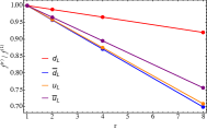
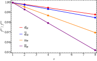
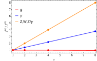
Figure 1: Scaling of the expanded PDFs with the parameter $r$, which multiplies $\alpha_{I=1,2,M}$. On the left, we show the left-handed quarks of the first generation, in the middle the right-handed quarks of the first generation, and on the right the vector bosons. One can clearly see that the expanded PDFs are linear in $\alpha_{I}$.

Given the resummed result for the SM PDFs, together with this first-order expansion, one can obtain a first estimate of the higher-order effects, and the convergence of electroweak perturbation theory. For this, we define the two ratios

$$r_{i}^{\rm noEW}(x,q)\equiv\frac{f^{\rm noEW}_{i}(x,q)}{f^{\rm SM}_{i}(x,q)}\,,\qquad r_{i}^{\rm SM,\alpha}(x,q)\equiv\frac{\left[f_{i}^{\rm SM}(x,q)\right]_{\alpha}}{f^{\rm SM}_{i}(x,q)}\,.$$ (22)

Defining the function $h_{i}(x,q)$ to be the difference between $[f_{i}^{\rm SM}]_{\alpha}$ and $f_{i}^{\rm SM}$ we can write

$$f_{i}^{\rm SM}(x,q)=f_{i}^{\rm noEW}(x,q)+g_{i}(x,q)+h_{i}(x,q)\,,$$ (23)

where $g_{i}(x,q)$ is the same function used in Eq. (14). As already discussed, the function $g_{i}(x,q)$ is of order $\alpha_{I}$, while the function $h_{i}(x,q)$ contains the resummed terms of $\alpha_{I}^{2}$ and higher. With these definitions, one can write

$$r_{i}^{\rm noEW}(x,q) =1-\frac{g_{i}(x,q)+h_{i}(x,q)}{f^{\rm SM}_{i}(x,q)}\sim 1+{\cal O}(\alpha_{I})\,,$$

$$r_{i}^{\rm SM,\alpha}(x,q) =1-\frac{h_{i}(x,q)}{f^{\rm SM}_{i}(x,q)}\sim 1+{\cal O}(\alpha_{I}^{2})\,.$$ (24)

Thus, the deviation from unity of the first ratio shows the size of the first-order correction, while the deviation of the second ratio shows the size of the higher-order corrections. Note that for PDFs for which $f^{\rm noEW}_{i}(x,q)$ vanishes (in our case the massive vector bosons) the first ratio vanishes, and the second ratio gives

$$r_{i}^{\rm SM,\alpha}(x,q) =1-\frac{h_{i}(x,q)}{g_{i}(x,q)}\sim 1+{\cal O}(\alpha_{I})$$ (25)

and is therefore an estimate of the size of the second-order term relative to the first-order term.

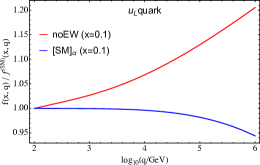
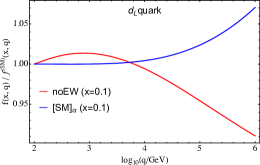
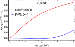
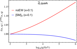
Figure 2: The ratio of the “noEW” and expanded SM PDFs relative to the PDF evaluated in the full SM for left-handed quarks.

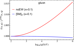
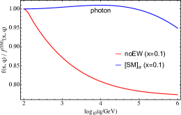
Figure 3: The ratio of the “noEW” and expanded SM PDFs relative to the PDF evaluated in the full SM for the massless vector bosons.

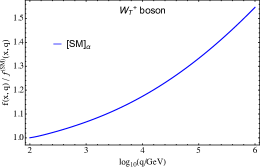
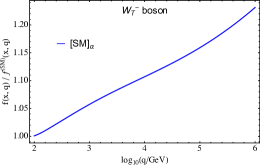
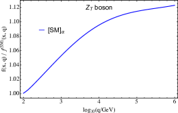
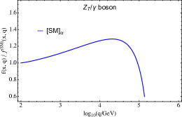
Figure 4: The ratio of the “noEW” and expanded SM PDFs relative to the PDF evaluated in the full SM for the transversely-polarized massive vector bosons.

The results are shown in Fig. 2 for left-handed up and down (anti)quarks. One can clearly see that at low values of $q$ the second-order correction is much smaller than the first-order correction, which is indicative of an absence of large logarithmic corrections. For $q\gtrsim 10^{4}$ GeV, however, the logarithmic contributions become noticeable, and the second-order correction grows relative to the first order, becoming comparable to the latter, at least for some of the PDFs, by $q\sim 10^{6}$ GeV. Notice that at high $q$ the left-handed up and down quarks move in opposite directions, to restore isospin symmetry asymptotically.

For the gluon and photon, the results are shown in Fig. 3. The gluon does not couple to the massive vector bosons directly, so the electroweak effect is strongly suppressed. Since the “noEW” PDFs include only QCD evolution, the photon does not evolve at all in that case, and receives a large first-order EW correction. In higher orders it can couple directly to the massive bosons, so its PDF is double-logarithmically sensitive to the ratio $m_{V}/q$. Therefore, although the higher-order corrections are much smaller than the first order for $q\sim q_{V}$, they grow much more rapidly at high values of $q$.

For massive vector bosons $r^{\rm noEW}(x,q)$ is zero, since their PDFs vanish when only QCD effects are included for $q>q_{V}$. Therefore, given our results, the validity of the perturbative expansion can only be studied through the ratio $r^{\rm SM,\alpha}(x,q)$, whose deviation from unity starts at first order in $\alpha_{I}$ as given in Eq. (25). In Fig. 4 one sees clearly the poor convergence of the perturbative expansion of massive boson PDFs: the deviation from unity is much larger than one power of $\alpha_{I}$, which of course is due to the double-logarithmic dependence on $m_{V}/q$. The ratio between the expanded PDF and the full PDF can deviate from unity by an amount in excess of 10%.

Given these PDFs and their expansions, one can find the first-order expansion of the SM luminosity

$$\left[{\cal L}^{\rm SM}_{AB}(x_{A},x_{B};Q)\right]_{\alpha} =f_{A}^{\rm noEW}(x_{A},Q)\,f_{B}^{\rm noEW}(x_{B},Q)+f_{A}^{\rm noEW}(x_{A},Q)\,g_{B}(x_{B},Q)$$

$$\quad+g_{A}(x_{A},Q)\,f_{B}^{\rm noEW}(x_{B},Q)\,.$$ (26)

From the definition Eq. (14) this obviously satisfies

$${\cal L}^{\rm SM}_{AB}(x_{A},x_{B};Q)-\left[{\cal L}^{\rm SM}_{AB}(x_{A},x_{B};Q)\right]_{\alpha}={\cal O}(\alpha_{I}^{2})\,.$$ (27)

Thus the difference in Eq. (27) can be used to add resummation terms to a NLO calculation, since it excludes all terms in the luminosity ${\cal L}^{\rm SM}_{AB}$ at ${\cal O}(1)$ and ${\cal O}(\alpha_{I})$ while including all LL terms of higher order.

Parton luminosities involving two massive gauge bosons (such as ${\cal L}_{ZZ}$, ${\cal L}_{W^{+}W^{-}}$) only start to contribute at order $\alpha_{I}^{2}$, since the PDF of each such boson is suppressed by one power of $\alpha_{I}$. This means that their effect is not included in the first-order expansion of the luminosity discussed above. However, vector-boson fusion (VBF) processes (those involving two massive gauge bosons in the initial state) can be significant numerically. For this reason, one might want to include their effects exactly at lowest order, and only rely on the LL approximation to predict their higher-order terms. This requires subtraction of the ${\cal O}(\alpha_{I}^{2})$ terms from ${\cal L}_{VV}$ when computing the expanded luminosity. The resulting modified expanded luminosity

$$\left[{\cal L}^{\rm SM}_{AB}(x_{A},x_{B};Q)\right]_{\alpha}^{\rm mod} =f_{A}^{\rm noEW}(x_{A},Q)\,f_{B}^{\rm noEW}(x_{B},Q)+f_{A}^{\rm noEW}(x_{A},Q)\,g_{B}(x_{B},Q)$$

$$\quad+g_{A}(x_{A},Q)\,f_{B}^{\rm noEW}(x_{B},Q)+g_{A}(x_{A},Q)\,g_{B}(x_{B},Q)\delta_{AB,VV}\,,$$ (28)

coinciding with Eq. (2) for all channels except $V_{T}V_{T}$, allows the inclusion of the exact lowest-order $V_{T}V_{T}$ contribution together with all resummed higher-order terms in that and the other channels. Thus to combine a fixed-order calculation including all EW effects at NLO, as well as the VBF process $V_{T}V_{T}$ at LO, which we denote by

$$\langle O\rangle_{\rm NLO+VV}\equiv\langle O\rangle_{\rm NLO}+\langle O\rangle^{\rm VV}_{\rm LO}\,,$$ (29)

one would compute

$$\langle O\rangle_{\rm NLO+VV+LL}=\langle O\rangle_{\rm NLO+VV}+\langle O\rangle_{\rm LL}-\left[\langle O\rangle_{\rm LL}\right]^{\rm mod}_{\alpha}\,.$$ (30)

where

$$\left[\langle O\rangle_{\rm LL}\right]^{\rm mod}_{\alpha}=\sum_{AB}\int\!{\rm d}\Phi_{n}\,O_{n}(\Phi_{n})\,\left[{\cal L}^{\rm SM}_{AB}(x_{A},x_{B};Q)\right]_{\alpha}^{\rm mod}B_{AB}(\Phi_{n})\,.$$ (31)

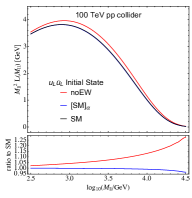
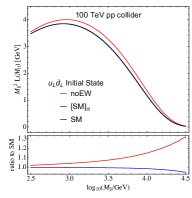
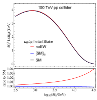
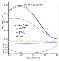
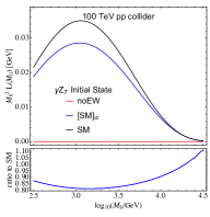
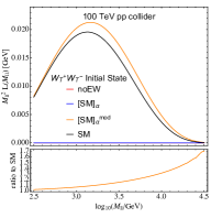
Figure 5: Plots showing luminosities for various choices of initial states. We show in black ${\cal L}^{\rm SM}$, in red ${\cal L}^{\rm noEW}$, in blue $\left[{\cal L}^{\rm SM}\right]_{\alpha}$ and for $V_{T}V_{T}$ initial states in orange $\left[{\cal L}^{\rm SM}\right]_{\alpha}^{\rm mod}$.

In Fig. 5 we show the results for a few selected parton luminosities

$${\cal L_{AB}}(M_{\ell\ell})=\int\!{\rm d}x_{A}\,{\rm d}x_{B}\,{\cal L}^{\rm SM}_{AB}\left(x_{A},x_{B};M_{\ell\ell}\right)\,\delta\left(M_{\ell\ell}-\sqrt{x_{1}x_{2}S}\right)\,,$$ (32)

for $pp$ collisions at $\sqrt{S}=100$ TeV, rescaled by the square of the invariant mass $M_{\ell\ell}$ to overcome the steeply falling nature of the functions. We show in black ${\cal L}^{\rm SM}$, in red ${\cal L}^{\rm noEW}$, in blue $\left[{\cal L}^{\rm SM}\right]_{\alpha}$ and for VV initial states in orange $\left[{\cal L}^{\rm SM}\right]_{\alpha}^{\rm mod}$. One can see that for left-handed quarks the difference between ${\cal L}^{\rm noEW}$ and ${\cal L}^{\rm SM}$ is larger than the difference between $\left[{\cal L}^{\rm SM}\right]_{\alpha}$ and ${\cal L}^{\rm SM}$ for all values of $M_{\ell\ell}$ considered, indicating that the double logarithms are not yet large enough to have $\alpha\ln^{2}(M_{\ell\ell}^{2}/m_{V}^{2})\gtrsim 1$. However, for $M_{\ell\ell}\gtrsim$ a few TeV the higher-order terms become significant. For right-handed quarks, there are no double logarithms and the coupling is smaller, so the convergence of the perturbation series is much faster. For the $\gamma\gamma$ initial state, recall that the “noEW” photon PDF is frozen at the matching scale $q_{V}=$ 100 GeV so the order $\alpha$ correction is large and dominates the expansion. For the $\gamma Z$ luminosity the higher-order terms are more significant. Finally, the $W^{+}W^{-}$ luminosity vanishes for $\left[{\cal L}^{\rm SM}\right]_{\alpha}$. Using the modified expansion reproduces the dominant features of the full luminosity, but higher order terms are still very important for $M_{\ell\ell}\gtrsim$ few TeV.

3 Resummation of logarithms in inclusive di-lepton production

In this section, we study the effects of higher-order leading logarithms in the process of fully inclusive di-lepton production. This will allow us to assess the correction from logarithmic resummation that needs to be applied to fixed-order calculations in order to achieve NLO+LL accuracy. Note, however, that we do not include the fixed-order calculation here.

The definition of fully inclusive di-lepton production was given in the introduction, but we will repeat it here for completeness. The inclusive process is defined to include a lepton-antilepton pair of any charge of a given generation and any number of extra gauge bosons in the final state. So to NLO EW accuracy, this process sums over the final states $\ell^{+}\ell^{-}(+V)$, $\ell^{+}\nu_{\ell}(+V)$, $\bar{\nu}_{\ell}\ell^{-}(+V)$, $\bar{\nu}_{\ell}\nu_{\ell}(+V)$. Here $\ell$ denotes, for example, the electron and $\nu_{\ell}$ the electron neutrino and the $(+V)$ denotes the possible addition of a $\gamma$, $Z$ or $W^{\pm}$ boson. Since we are summing over both electrons and neutrinos, and we are including the radiation of extra electroweak gauge bosons, the final state of this process is SU(2) symmetric, as required. In order to regulate the strong enhancement of forward lepton production in vector boson fusion, we impose a cut on the transverse momentum of each lepton $p_{T}>100$ GeV. This implies that the accessible di-lepton invariant masses are $M_{\ell\ell}>200$ GeV.

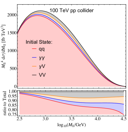
Figure 6: The differential cross section $M_{\ell\ell}^{4}{\rm d}\sigma/{\rm d}M_{\ell\ell}(p_{T\ell}>100$ GeV) for a 100 TeV collider, showing the makeup of the total cross section in terms of the individual initial states.

To compute the partonic Born cross section $B_{AB}(\widehat{\Phi}_{n})$ in Eq. (8), one relates it to the square of the relevant matrix element via

$$B_{AB}(\Phi_{n})\equiv\frac{1}{4p_{A}\!\cdot\!p_{B}}\left|M(AB\to\ell\ell)\right|^{2}\,,$$ (33)

where $\ell$ denotes either a charged lepton or a neutrino. As discussed in Section 1, for the initial states $A$ and $B$ one needs $q\bar{q}$ of all possible quark flavors and helicities, as well as $VV$, where $V$ can be any one of the electroweak gauge bosons, $\gamma,Z^{0},W^{\pm},$ or the mixed $\gamma/Z^{0}$ representing interference contributions. The contributions of initial-state leptons, longitudinal gauge bosons and Higgs bosons are much smaller and will be neglected. Details of the cross-section calculations are given in the Appendix.

The leading-logarithmic differential cross section ${\rm d}\sigma/{\rm d}M_{\ell\ell}$ is shown for a 100 TeV $pp$ collider in Fig 6. In order to make the plot easier to read, we have multiplied the differential cross section by $M_{\ell\ell}^{4}$ to overcome its steeply falling nature. We have stacked the contributions of the various initial states $q\bar{q}$, $\gamma\gamma$, $\gamma V_{T}$ and $V_{T}V_{T}$ (where $V_{T}$ now denotes a sum over massive transversely polarized electroweak gauge bosons) on top of each other. In the lower part of the plot, we show the ratio to the total contribution, giving a better estimate of the relative size of each contribution. One can see that the dominant contribution is from the $q\bar{q}$ initial states, but the relative size of the initial states with two vector bosons grows with increasing $M_{\ell\ell}$. For a 100 TeV collider, the contributions with vector bosons in the initial state are around 25% for $M_{\ell\ell}=10^{4.5}$ GeV $\sim 30$ TeV.

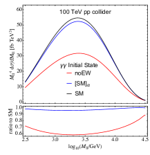
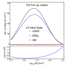
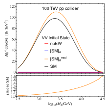
Figure 7: The expansion of the various contributions to $M_{\ell\ell}^{4}{\rm d}\sigma/{\rm d}M_{\ell\ell}(p_{T\ell}>100$ GeV) for a 100 TeV collider. We show in black the result obtained using ${\cal L}^{\rm SM}$, in red that using ${\cal L}^{\rm noEW}$, in blue that using $\left[{\cal L}^{\rm SM}\right]_{\alpha}$ and for $V_{T}V_{T}$ initial states in orange that using $\left[{\cal L}^{\rm SM}\right]_{\alpha}^{\rm mod}$.

Next, we take each of the four contributions and investigate their convergence under EW perturbation theory. For this, we compare the result of the LL-resummed cross section $M_{\ell\ell}^{4}{\rm d}\sigma_{\rm LL}/{\rm d}M_{\ell\ell}$ with its first-order expansion $[M_{\ell\ell}^{4}{\rm d}\sigma_{\rm LL}/{\rm d}M_{\ell\ell}]_{\alpha}$ for the various initial states. The results are shown for a 100 TeV pp collider in Fig. 7, where in black we show the resummed result, and in blue its first-order expansion. The difference between these two is the correction that should be added to a fixed-order calculation to achieve NLO+LL accuracy. For comparison, we also show in red the “noEW” result. The difference between the blue and red curves shows the logarithmically enhanced order-$\alpha$ contribution. As one can see, for the $q\bar{q}$ channel, the expansion of the LL result is quite close to the full LL result, indicating that the higher-order corrections are quite small. This is due to two facts: First, the right-handed quarks do not receive any double-logarithmic contributions (and their single logarithmic terms come with coupling constant $\alpha_{1}$ rather than $\alpha_{2}$). Second, since sea quarks are mostly iso-singlet, the double logarithms only arise from iso-vector contributions of the valence quarks. Each of these facts reduces the double logarithmic effect by roughly a factor of 2, such that overall the effect is smaller by a factor of 4 compared to an individual $q_{L}\bar{q}_{L}$ parton luminosity. Note that one of these factors of two would be absent for a $p\bar{p}$ collider, so one would expect the effect to be larger there by a factor of 2.

For $\gamma\gamma$ initial states, one needs to keep in mind that our definition of $f^{\rm noEW}$ does not include any QED evolution for $q>q_{V}$. This means that the photon PDF freezes out at the scale $q_{V}$ for this PDF. Since the effect of the evolution is of the same size as the value of the PDF at $q=q_{V}$, the first order (difference of red and black) gives an ${\cal O}(1)$ effect. The second order (difference of blue and black) is considerably smaller than the first order for all values of $M_{\ell\ell}$, but from the absolute value of the correction it is also clear that the expansion parameter is much larger than $\alpha_{\rm em}/\pi$ as one might naively expect. For example, for $M_{\ell\ell}\sim 1$ TeV, the second-order correction is almost 5%.

Any process with massive bosons in the initial states is suppressed by one power of $\alpha$ for each. Therefore the “noEW” luminosity vanishes for $\gamma V_{T}$ and $V_{T}V_{T}$, and for $V_{T}V_{T}$ the [SM]_α luminosity also vanishes, as indicated by the red and blue lines in the last two plots. However, for $\gamma V_{T}$ the second-order correction (the difference between the blue and the black line) reaches tens of percent at high $M_{\ell\ell}$, indicating that the higher order perturbative corrections are significant. For $V_{T}V_{T}$ initial states, we also show in orange the result of the modified expansion Eq. (2), which includes the leading ${\cal O}(\alpha^{2})$ term. The difference between the orange and black curve denotes ${\cal O}(\alpha^{3})$ terms, which are tens of percent of the leading ${\cal O}(\alpha^{2})$ terms, indicating again a poorly convergent perturbation series.

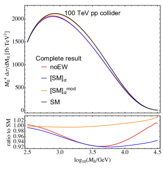
Figure 8: The expansion of the complete result $M_{\ell\ell}^{4}{\rm d}\sigma/{\rm d}M_{\ell\ell}(p_{T\ell}>100$ GeV) for a 100 TeV collider. The colors are the same as in Fig. 7.

Putting these results together, we show in Fig. 8 the combination of the various channels. One can see that perturbation theory is not very well behaved and for $M_{\ell\ell}\gtrsim 5$ TeV, the second order correction is essentially of the same size as the first order correction (there is an accidental cancellation for very large $M_{\ell\ell}$ which makes the first order correction become small). The overall effect of the corrections of order $\alpha_{I}^{2}$ and higher for $M_{\ell\ell}\gtrsim$ a few TeV is of the order of 5%. Most of this comes from the VBF processes, so the correction to the modified expansion Eq. (2) is much smaller.

To understand how these results depend on the center-of-mass energy of the collider, we also show results at 27 TeV, which is the energy that might be achieved by a high-energy upgrade of the LHC using novel magnet technology [51], and a fictitious 1 PeV collider. In Fig. 9 the relative importance of the various channels is shown. One obvious effect is that at high energies one has access to larger values of the di-lepton invariant mass, for which the logarithmic enhancement is stronger. However, even at fixed invariant mass the relative importance of the initial states with vector bosons is diminished (enhanced) for a 27 TeV (1 PeV) collider. This is because at higher energies one is probing smaller values of $x$, and the vector boson PDFs, like that of the gluon, rise rapidly with decreasing $x$. For a 1 PeV collider at the highest accessible di-lepton invariant mass, the contribution of vector boson initial states is almost 50% of the total cross section.

Finally, we study the convergence of perturbation theory for individual channels for a 27 TeV and 1 PeV collider in Figs. 10 and 11, respectively, and the complete result in Fig. 12. Qualitatively the effects are the same as for a 100 TeV collider, but the overall size of the effects are decreased (increased) for the 27 TeV (1 PeV) collider.

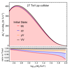
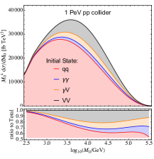
Figure 9: The differential cross section $M_{\ell\ell}^{4}{\rm d}\sigma/{\rm d}M_{\ell\ell}(p_{T\ell}>100$ GeV) for a $27$ TeV and $1$ PeV collider, showing the makeup of the total cross section in terms of the individual initial states.

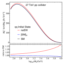
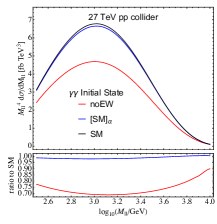
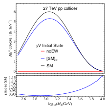
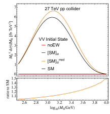
Figure 10: The expansion of the various contributions to $M_{\ell\ell}^{4}{\rm d}\sigma/{\rm d}M_{\ell\ell}(p_{T\ell}>100$ GeV) for a 27 TeV collider. The colors are the same as in Fig. 7.

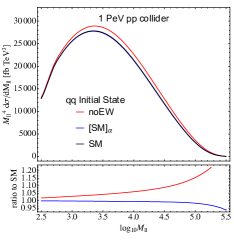
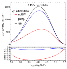
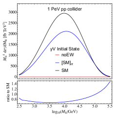
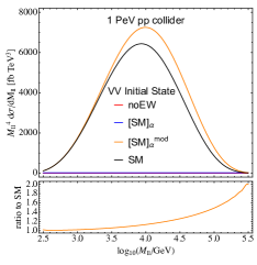
Figure 11: The expansion of the various contributions to $M_{\ell\ell}^{4}{\rm d}\sigma/{\rm d}M_{\ell\ell}(p_{T\ell}>100$ GeV) for a 1 PeV collider. The colors are the same as in Fig. 7.

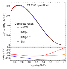
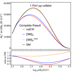
Figure 12: The expansion of the complete result $M_{\ell\ell}^{4}{\rm d}\sigma/{\rm d}M_{\ell\ell}(p_{T\ell}>100$ GeV) for a 27 TeV and 1 PeV collider. The colors are the same as in Fig. 7

4 Conclusions

A fuller understanding of electroweak effects is becoming essential as the energy frontier of particle physics moves beyond the scale of electroweak symmetry breaking. In this paper we have focused on the effects of large logarithmic terms associated with initial-state emission of electroweak bosons. Since all types of colliders necessarily have beams that are not symmetric with respect to weak isospin, there are double-logarithmic enhancements of electroweak corrections associated with initial-state radiation that do not cancel, even in fully inclusive processes, and become increasingly important at high energies. These enhanced terms can be resummed to all orders by means of DGLAP-type evolution equations involving parton distribution functions for all the fields of the Standard Model. The evolution equations also resum important classes of single logarithms (but not all of them), including those associated with fermion, gluon and U(1) gauge boson emission.

We have proposed a method for combining resummation with fixed-order electroweak calculations, without double counting of terms already included. This is done by expanding the evolution equations to fixed order in the electroweak couplings and computing the terms that need to be subtracted to avoid double counting. The remaining terms then provide a resummed estimate of the higher-order effects beyond those that have been computed exactly in fixed order. The relative size of the first- and higher-order terms provides an indication of the convergence of electroweak perturbation theory.

In order to combine resummed and fixed-order calculations without double counting, one needs to specify carefully the terms included in each case. In particular, the PDF sets used for the latter should not include terms present in the electroweak evolution equations used for the former. We therefore propose a “noEW” scheme for fixed-order calculations, in which there is no U(1)_em evolution above the electroweak scale. In particular, the photon PDF used in the fixed-order calculation is frozen at a matching scale $q_{V}\sim m_{V}\sim 100$ GeV, and the resummation takes care of all the photon evolution above that scale.

Using this scheme, we have presented comparisons between “noEW” results, the full leading-logarithmic resummation (SM) and the resummed results expanded to fixed order ([SM]_α), at the level of PDFs, parton-parton luminosities and fully-inclusive di-lepton cross sections. The difference between [SM]_α and “noEW” represents the part that should be replaced by an exact order-$\alpha$ calculation for improved precision. The difference between SM and [SM]_α then indicates the extra contribution from the resummation of enhanced terms of yet higher orders. Our results are shown mainly in the context of a future $pp$ collider of center-of-mass energy 100 TeV, but we also show some effects at a possible 27 TeV high-energy upgrade of the LHC and at much higher energy.

A notable feature of our findings is that there are relatively large contributions to the PDFs of the electroweak vector bosons beyond order $\alpha$, reaching tens of percent beyond scales of $\sim 10$ TeV. This is reflected in their contributions to luminosities and the di-lepton cross section. Even at fixed invariant mass, the relative importance of the initial states with vector bosons increases with collider energy. This is because at higher energies one is probing smaller values of $x$. Since the contributions of vector boson fusion processes begin at order $\alpha^{2}$, one may wish to make an extra subtraction of this piece from the resummation, resulting in a scheme we call [SM]${}^{\rm mod}_{\alpha}$. In this scheme one can include the exact lowest-order VBF contribution, the difference between SM and [SM]${}^{\rm mod}_{\alpha}$ then indicating the effect of remaining resummed terms. We find that the latter are still quite significant, again reaching tens of percent beyond scales of $\sim 10$ TeV.

Our approach naturally invites a number of future developments. Foremost of these would be the inclusion of exact order-$\alpha$ calculations in the way we have proposed, together with order-$\alpha^{2}$ VBF contributions. The fully-inclusive di-lepton process that we have considered is not experimentally relevant, owing to the presence of unobservable neutrinos. This could be rectified either by including Sudakov factors for a fully exclusive $e^{+}e^{-}$ or $\mu^{+}\mu^{-}$ final state, or by computing fragmentation functions for the inclusive production of charged leptons. Ultimately, fully exclusive final states containing all combinations of jets, leptons, photons and massive bosons could be simulated by an event generator based on complete Standard Model evolution equations for initial- and final-state parton showers.

Appendix A The partonic Born cross sections for di-lepton production

The expressions for the Born cross sections with $AB=q\bar{q}$ and $AB=W^{+}W^{-}$ are given in Table 2,

$AB\to\ell\bar{\ell}^{\prime}$	$B_{AB}$
$q_{L/R}\,\bar{q}_{L/R}\to\ell_{L/R}\,\bar{\ell}_{L/R}$	$\frac{8\pi^{2}}{s}\,f_{L/R,L/R}(s,t,u)\,\left(\alpha_{1}Y_{q}Y_{\ell}+\alpha_{2}I_{q}I_{\ell}\right)^{2}$
$q_{L/R}\,\bar{q}_{L/R}\to\ell_{R/L}\,\bar{\ell}_{R/L}$	$\frac{8\pi^{2}}{s}\,f_{L/R,R/L}(s,t,u)\,\alpha_{1}^{2}Y_{q}^{2}Y_{\ell}^{2}$
$q_{L}\,\bar{q}_{L}^{\prime}\to\ell_{L}\,\bar{\ell}_{L}^{\prime}$	$\frac{8\pi^{2}}{s}\,f_{C,L}(s,t,u)\,\alpha_{2}^{2}$
$W^{+}\,W^{-}\to e_{L}\bar{e}_{L}$	$\frac{8\pi^{2}}{s}\,f_{(+,-)}^{(1)}(s,t,u)\,\alpha_{2}^{2}$
$W^{+}\,W^{-}\to\nu_{L}\bar{\nu}_{L}$	$\frac{8\pi^{2}}{s}\,f_{(+,-)}^{(2)}(s,t,u)\,\alpha_{2}^{2}$

Table 2: Born cross sections for $q\bar{q}$ and $W^{+}W^{-}$ going to lepton pairs. Here $e$ stands for the charged lepton. The cross sections for $BA\to\ell\bar{\ell}^{\prime}$ are the same as $AB\to\ell\bar{\ell}^{\prime}$ with $t\leftrightarrow u$.

with the various functional dependences on the Mandelstam variables $s,t,u$,

$$s=(p_{A}+p_{B})^{2}\,,\qquad t=(p_{A}-p_{\ell})^{2}\,,\qquad u=(p_{B}-p_{\ell})^{2}\,,$$ (34)

given by

$$f_{L/R,L/R}(s,t,u) =\frac{4}{3}\frac{u^{2}}{s^{2}}$$ (35)

$$f_{L/R,R/L}(s,t,u) =\frac{4}{3}\frac{t^{2}}{s^{2}}$$

$$f_{C,L}(s,t,u) =\frac{1}{3}\frac{u^{2}}{s^{2}}$$

$$f_{(+,-)}^{(1)}(s,t,u) =\frac{t}{4u}\frac{t^{2}+u^{2}}{s^{2}}$$

$$f_{(+,-)}^{(2)}(s,t,u) =\frac{u}{4t}\frac{t^{2}+u^{2}}{s^{2}}\,.$$

For the scattering involving neutral gauge bosons in the initial state one can either work in the unbroken basis (where the neutral bosons required are $B$, $W_{3}$ or mixed $M=B/W_{3}$) or in the broken basis (where the neutral bosons required are $\gamma$, $Z$ or mixed $\tilde{M}=\gamma/Z$). For the unbroken basis the results are given in Table 3 with

$$f_{N}(s,t,u) =\frac{t^{2}+u^{2}}{ut}$$ (36)

$$f_{(\pm,3)}(s,t,u) =\frac{1}{8}\frac{u^{2}+t^{2}}{ut}\frac{(t-u)^{2}}{s^{2}}$$

$$f_{(\pm,B)}(s,t,u) =\frac{1}{8}\frac{u^{2}+t^{2}}{ut}$$

$$f_{(\pm,M)}(s,t,u) =\pm\frac{1}{8}\frac{u^{2}+t^{2}}{ut}\frac{t-u}{s}\,,$$

while for the broken basis the results are in Table 4 with

$$f_{+,\gamma}(s,t,u) =\frac{1}{2}\frac{u^{2}+t^{2}}{s^{2}}\frac{u}{t}$$ (37)

$$f_{-,\gamma}(s,t,u) =\frac{1}{2}\frac{u^{2}+t^{2}}{s^{2}}\frac{t}{u},$$

$$f_{+,Z}(s,t,u) =\frac{1}{8}\frac{u^{2}+t^{2}}{ut}\left(\frac{s+2c_{W}^{2}u}{c_{W}s_{W}s}\right)^{2}$$

$$f_{-,Z}(s,t,u) =\frac{1}{8}\frac{u^{2}+t^{2}}{ut}\left(\frac{s+2c_{W}^{2}t}{c_{W}s_{W}s}\right)^{2}$$

$$f_{+,\tilde{M}}(s,t,u) =\frac{1}{4}\frac{u^{2}+t^{2}}{st}\frac{s+2c_{W}^{2}u}{c_{W}s_{W}s}$$

$$f_{-,\tilde{M}}(s,t,u) =\frac{1}{4}\frac{u^{2}+t^{2}}{su}\frac{s+2c_{W}^{2}t}{c_{W}s_{W}s}\,,$$

where $s_{W}$ and $c_{W}$ represent the sine and cosine of the weak mixing angle, respectively.

$AB\to\ell\bar{\ell}^{\prime}$	$B_{AB}$
$W^{3}\,W^{3}\to\ell\bar{\ell}$	$\frac{8\pi^{2}}{s}\,f_{N}(s,t,u)\,\alpha_{2}^{2}\,I_{\ell}^{4}$
$W^{3}\,B\to\ell\bar{\ell}$	$\frac{8\pi^{2}}{s}\,f_{N}(s,t,u)\,\alpha_{1}\,\alpha_{2}\,Y_{\ell}^{2}\,I_{\ell}^{2}$
$W^{3}\,M\to\ell\bar{\ell}$	$\frac{8\pi^{2}}{s}\,f_{N}(s,t,u)\,\sqrt{\alpha_{1}\alpha_{2}}\,\alpha_{2}\,Y_{\ell}\,I_{\ell}^{3}$
$B\,B\to\ell\bar{\ell}$	$\frac{8\pi^{2}}{s}\,f_{N}(s,t,u)\,\alpha_{1}^{2}\,Y_{\ell}^{4}$
$B\,M\to\ell\bar{\ell}$	$\frac{8\pi^{2}}{s}\,f_{N}(s,t,u)\,\sqrt{\alpha_{1}\alpha_{2}}\,\alpha_{1}\,Y_{\ell}^{3}\,I_{\ell}$
$M\,M\to\ell\bar{\ell}$	$\frac{8\pi^{2}}{s}\,f_{N}(s,t,u)\,\alpha_{1}\,\alpha_{2}\,Y_{\ell}^{2}\,I_{\ell}^{2}$
$W^{\pm}\,W^{3}\to\ell_{L}\bar{\ell}^{\prime}_{L}$	$\frac{8\pi^{2}}{s}\,f_{(\pm,3)}(s,t,u)\,\alpha_{2}^{2}$
$W^{\pm}\,B\to\ell_{L}\bar{\ell}^{\prime}_{L}$	$\frac{8\pi^{2}}{s}\,f_{(\pm,B)}(s,t,u)\,\alpha_{1}\,\alpha_{2}$
$W^{\pm}\,M\to\ell_{L}\bar{\ell}^{\prime}_{L}$	$\frac{8\pi^{2}}{s}\,f_{(\pm,M)}(s,t,u)\,\sqrt{\alpha_{1}\alpha_{2}}\,\alpha_{2}$

Table 3: Born cross sections for $VV$ in the unbroken basis going to lepton pairs. Here $M$ stands for the mixed $B/W_{3}$ PDF. The cross sections for $BA\to\ell\bar{\ell}^{\prime}$ are the same as $AB\to\ell\bar{\ell}^{\prime}$ with $t\leftrightarrow u$.

$AB\to\ell\bar{\ell}^{\prime}$	$B_{AB}$
$\gamma\,\gamma\to\ell\bar{\ell}$	$\frac{8\pi^{2}}{s}\,f_{N}(s,t,u)\,\alpha^{2}\,Q_{\ell}^{4}$
$\gamma\,Z\to\ell\bar{\ell}$	$\frac{8\pi^{2}}{s}\,f_{N}(s,t,u)\,\alpha^{2}\,Q_{\ell}^{2}\,R_{\ell}^{2}$
$\gamma\,\tilde{M}\to\ell\bar{\ell}$	$\frac{8\pi^{2}}{s}\,f_{N}(s,t,u)\,\alpha^{2}\,Q_{\ell}^{3}\,R_{\ell}$
$Z\,Z\to\ell\bar{\ell}$	$\frac{8\pi^{2}}{s}\,f_{N}(s,t,u)\,\alpha^{2}\,R_{\ell}^{4}$
$Z\,\tilde{M}\to\ell\bar{\ell}$	$\frac{8\pi^{2}}{s}\,f_{N}(s,t,u)\,\alpha^{2}\,\,Q_{\ell}\,R_{\ell}^{3}$
$\tilde{M}\,\tilde{M}\to\ell\bar{\ell}$	$\frac{8\pi^{2}}{s}\,f_{N}(s,t,u)\,\alpha^{2}\,Q_{\ell}^{2}\,R_{\ell}^{2}$
$W^{\pm}\,\gamma\to\ell_{L}\bar{\ell}^{\prime}_{L}$	$\frac{8\pi^{2}}{s}\,f_{(\pm,\gamma)}(s,t,u)\,\alpha\,\alpha_{2}$
$W^{\pm}\,Z\to\ell_{L}\bar{\ell}^{\prime}_{L}$	$\frac{8\pi^{2}}{s}\,f_{(\pm,Z)}(s,t,u)\,\alpha\,\alpha_{2}$
$W^{\pm}\,\tilde{M}\to\ell_{L}\bar{\ell}^{\prime}_{L}$	$\frac{8\pi^{2}}{s}\,f_{(\pm,\tilde{M})}(s,t,u)\,\alpha\,\alpha_{2}$

Table 4: Born cross sections for $VV$ in the broken basis going to lepton pairs. Here $\tilde{M}$ stands for the mixed $\gamma/Z$ PDF. The cross sections for $BA\to\ell\bar{\ell}^{\prime}$ are the same as $AB\to\ell\bar{\ell}^{\prime}$ with $t\leftrightarrow u$.

References

- [1] N. Arkani-Hamed, T. Han, M. Mangano and L.-T. Wang, Physics opportunities of a 100 TeV proton-proton collider, Phys. Rept. 652 (2016) 1–49, [1511.06495].
- [2] M. L. Mangano et al., Physics at a 100 TeV pp collider: Standard Model processes, 1607.01831.
- [3] P. Ciafaloni and D. Comelli, Sudakov enhancement of electroweak corrections, Phys. Lett. B446 (1999) 278–284, [hep-ph/9809321].
- [4] P. Ciafaloni and D. Comelli, Electroweak Sudakov form-factors and nonfactorizable soft QED effects at NLC energies, Phys. Lett. B476 (2000) 49–57, [hep-ph/9910278].
- [5] M. Ciafaloni, P. Ciafaloni and D. Comelli, Bloch-Nordsieck violating electroweak corrections to inclusive TeV scale hard processes, Phys. Rev. Lett. 84 (2000) 4810–4813, [hep-ph/0001142].
- [6] M. Ciafaloni, P. Ciafaloni and D. Comelli, Electroweak double logarithms in inclusive observables for a generic initial state, Phys. Lett. B501 (2001) 216–222, [hep-ph/0007096].
- [7] M. Ciafaloni, P. Ciafaloni and D. Comelli, Electroweak Bloch-Nordsieck violation at the TeV scale: ’Strong’ weak interactions?, Nucl. Phys. B589 (2000) 359–380, [hep-ph/0004071].
- [8] M. Ciafaloni, P. Ciafaloni and D. Comelli, Enhanced electroweak corrections to inclusive boson fusion processes at the TeV scale, Nucl. Phys. B613 (2001) 382–406, [hep-ph/0103316].
- [9] M. Ciafaloni, P. Ciafaloni and D. Comelli, Towards collinear evolution equations in electroweak theory, Phys. Rev. Lett. 88 (2002) 102001, [hep-ph/0111109].
- [10] P. Ciafaloni, D. Comelli and A. Vergine, Sudakov electroweak effects in transversely polarized beams, JHEP 07 (2004) 039, [hep-ph/0311260].
- [11] P. Ciafaloni and D. Comelli, Electroweak evolution equations, JHEP 11 (2005) 022, [hep-ph/0505047].
- [12] P. Ciafaloni and D. Comelli, The Importance of weak bosons emission at LHC, JHEP 09 (2006) 055, [hep-ph/0604070].
- [13] M. Ciafaloni, P. Ciafaloni and D. Comelli, Electroweak double-logs at small x, JHEP 05 (2008) 039, [0802.0168].
- [14] P. Ciafaloni and A. Urbano, Infrared weak corrections to strongly interacting gauge bosons scattering, Phys. Rev. D81 (2010) 085033, [0902.1855].
- [15] P. Ciafaloni, D. Comelli, A. Riotto, F. Sala, A. Strumia and A. Urbano, Weak Corrections are Relevant for Dark Matter Indirect Detection, JCAP 1103 (2011) 019, [1009.0224].
- [16] S. Forte et al., The Standard Model from LHC to future colliders, Eur. Phys. J. C75 (2015) 554, [1505.01279].
- [17] C. W. Bauer, N. Ferland and B. R. Webber, Standard Model Parton Distributions at Very High Energies, JHEP 08 (2017) 036, [1703.08562].
- [18] V. S. Fadin, L. N. Lipatov, A. D. Martin and M. Melles, Resummation of double logarithms in electroweak high-energy processes, Phys. Rev. D61 (2000) 094002, [hep-ph/9910338].
- [19] J. H. Kühn, A. A. Penin and V. A. Smirnov, Summing up subleading Sudakov logarithms, Eur. Phys. J. C17 (2000) 97–105, [hep-ph/9912503].
- [20] A. Denner and S. Pozzorini, One loop leading logarithms in electroweak radiative corrections. 1. Results, Eur. Phys. J. C18 (2001) 461–480, [hep-ph/0010201].
- [21] A. Denner and S. Pozzorini, One loop leading logarithms in electroweak radiative corrections. 2. Factorization of collinear singularities, Eur. Phys. J. C21 (2001) 63–79, [hep-ph/0104127].
- [22] B. Feucht, J. H. Kühn, A. A. Penin and V. A. Smirnov, Two loop Sudakov form-factor in a theory with mass gap, Phys. Rev. Lett. 93 (2004) 101802, [hep-ph/0404082].
- [23] B. Jantzen, J. H. Kühn, A. A. Penin and V. A. Smirnov, Two-loop electroweak logarithms, Phys. Rev. D72 (2005) 051301, [hep-ph/0504111].
- [24] B. Jantzen, J. H. Kühn, A. A. Penin and V. A. Smirnov, Two-loop electroweak logarithms in four-fermion processes at high energy, Nucl. Phys. B731 (2005) 188–212, [hep-ph/0509157].
- [25] M. Beccaria, F. M. Renard and C. Verzegnassi, Top quark production at future lepton colliders in the asymptotic regime, Phys. Rev. D63 (2001) 053013, [hep-ph/0010205].
- [26] M. Hori, H. Kawamura and J. Kodaira, Electroweak Sudakov at two loop level, Phys. Lett. B491 (2000) 275–279, [hep-ph/0007329].
- [27] W. Beenakker and A. Werthenbach, Electroweak two loop Sudakov logarithms for on-shell fermions and bosons, Nucl. Phys. B630 (2002) 3–54, [hep-ph/0112030].
- [28] A. Denner, M. Melles and S. Pozzorini, Two loop electroweak angular dependent logarithms at high-energies, Nucl. Phys. B662 (2003) 299–333, [hep-ph/0301241].
- [29] S. Pozzorini, Next to leading mass singularities in two loop electroweak singlet form-factors, Nucl. Phys. B692 (2004) 135–174, [hep-ph/0401087].
- [30] B. Jantzen and V. A. Smirnov, The Two-loop vector form-factor in the Sudakov limit, Eur. Phys. J. C47 (2006) 671–695, [hep-ph/0603133].
- [31] J.-y. Chiu, F. Golf, R. Kelley and A. V. Manohar, Electroweak Sudakov corrections using effective field theory, Phys. Rev. Lett. 100 (2008) 021802, [0709.2377].
- [32] J.-y. Chiu, F. Golf, R. Kelley and A. V. Manohar, Electroweak Corrections in High Energy Processes using Effective Field Theory, Phys. Rev. D77 (2008) 053004, [0712.0396].
- [33] J.-y. Chiu, R. Kelley and A. V. Manohar, Electroweak Corrections using Effective Field Theory: Applications to the LHC, Phys. Rev. D78 (2008) 073006, [0806.1240].
- [34] J.-y. Chiu, A. Fuhrer, A. H. Hoang, R. Kelley and A. V. Manohar, Soft-Collinear Factorization and Zero-Bin Subtractions, Phys. Rev. D79 (2009) 053007, [0901.1332].
- [35] J.-y. Chiu, A. Fuhrer, A. H. Hoang, R. Kelley and A. V. Manohar, Using SCET to calculate electroweak corrections in gauge boson production, PoS EFT09 (2009) 009, [0905.1141].
- [36] J.-y. Chiu, A. Fuhrer, R. Kelley and A. V. Manohar, Factorization Structure of Gauge Theory Amplitudes and Application to Hard Scattering Processes at the LHC, Phys. Rev. D80 (2009) 094013, [0909.0012].
- [37] J.-y. Chiu, A. Fuhrer, R. Kelley and A. V. Manohar, Soft and Collinear Functions for the Standard Model, Phys. Rev. D81 (2010) 014023, [0909.0947].
- [38] A. Fuhrer, A. V. Manohar, J.-y. Chiu and R. Kelley, Radiative Corrections to Longitudinal and Transverse Gauge Boson and Higgs Production, Phys. Rev. D81 (2010) 093005, [1003.0025].
- [39] S. Kallweit, J. M. Lindert, P. Maierhöfer, S. Pozzorini and M. Schönherr, NLO electroweak automation and precise predictions for W+multijet production at the LHC, JHEP 04 (2015) 012, [1412.5157].
- [40] S. Kallweit, J. M. Lindert, P. Maierhöfer, S. Pozzorini and M. Schönherr, NLO QCD+EW predictions for V + jets including off-shell vector-boson decays and multijet merging, JHEP 04 (2016) 021, [1511.08692].
- [41] S. Kallweit, J. M. Lindert, S. Pozzorini and M. Schönherr, NLO QCD+EW predictions for diboson signatures at the LHC, JHEP 11 (2017) 120, [1705.00598].
- [42] F. Granata, J. M. Lindert, C. Oleari and S. Pozzorini, NLO QCD+EW predictions for HV and HV +jet production including parton-shower effects, JHEP 09 (2017) 012, [1706.03522].
- [43] M. Chiesa, N. Greiner, M. Schönherr and F. Tramontano, Electroweak corrections to diphoton plus jets, JHEP 10 (2017) 181, [1706.09022].
- [44] V. N. Gribov and L. N. Lipatov, Deep inelastic e p scattering in perturbation theory, Sov. J. Nucl. Phys. 15 (1972) 438–450.
- [45] Y. L. Dokshitzer, Calculation of the Structure Functions for Deep Inelastic Scattering and e+ e- Annihilation by Perturbation Theory in Quantum Chromodynamics., Sov. Phys. JETP 46 (1977) 641–653.
- [46] G. Altarelli and G. Parisi, Asymptotic Freedom in Parton Language, Nucl. Phys. B126 (1977) 298–318.
- [47] J. Chen, T. Han and B. Tweedie, Electroweak Splitting Functions and High Energy Showering, JHEP 11 (2017) 093, [1611.00788].
- [48] C. Schmidt, J. Pumplin, D. Stump and C. P. Yuan, CT14QED parton distribution functions from isolated photon production in deep inelastic scattering, Phys. Rev. D93 (2016) 114015, [1509.02905].
- [49] A. Manohar, P. Nason, G. P. Salam and G. Zanderighi, How bright is the proton? A precise determination of the photon parton distribution function, Phys. Rev. Lett. 117 (2016) 242002, [1607.04266].
- [50] A. V. Manohar, P. Nason, G. P. Salam and G. Zanderighi, The Photon Content of the Proton, 1708.01256.
- [51] D. Tommasini et al., The 16 T Dipole Development Program for FCC, IEEE Trans. Appl. Supercond. 27 (2016) 4000405.