Imprints of Cosmic Rays in Multifrequency Observations of the Interstellar Emission

Abstract

Ever since the discovery of Cosmic Rays (CRs), significant advancements have been made in modeling their propagation in the Galaxy and in the Heliosphere. However, propagation models suffer from degeneracy of many parameters. To complicate the picture the precision of recent data have started challenging existing models.
To tackle these issues we use available multifrequency observations of the interstellar emission from radio to gamma rays, together with direct CR measurements, to study local interstellar spectra (LIS) and propagation models.
As a result, the electron LIS is characterized without any assumption on solar modulation, and favorite propagation models are put forward. More precisely, our analysis leads to the following main conclusions: (1) the electron injection spectrum needs at least a break below a few GeV; (2) even though consistent with direct CR measurements, propagation models producing a LIS with large all-electron density from a few hundreds of MeV to a few GeV are disfavored by both radio and gamma-ray observations; (3) the usual assumption that direct CR measurements, after accounting for solar modulation, are representative of the proton LIS in our $\sim$1 kpc region is challenged by the observed local gamma-ray HI emissivity.
We provide the resulting proton LIS, all-electron LIS, and propagation parameters, based on synchrotron, gamma-ray, and direct CR data. A plain diffusion model and a tentative diffusive-reacceleration model are put forward. The various models are investigated in the inner-Galaxy region in X-rays and gamma rays. Predictions of the interstellar emission for future gamma-ray instruments (e-ASTROGAM and AMEGO) are derived.

1 Introduction

The Milky Way is permeated by Cosmic Rays (CRs) that diffuse and interact within the Galaxy producing diffuse interstellar emission from radio to gamma rays. While significant advancements have been made by studying CRs through their diffuse interstellar emission either at radio (e.g. Strong et al., 2011) or at gamma-ray energies (e.g. Abdo et al., 2009; Ackermann et al., 2012) independently, these studies are unavoidably affected by uncertainties. However, the CRs responsible for the radio emission are the same producing also the gamma-ray emission. In this work we take advantage of this property with the aim of constraining CRs by looking at the interstellar emission in radio and gamma-ray energies simultaneously. This approach provides a handle on both sides of the electromagnetic spectrum in understanding CRs, thereby leaving less room to uncertainties. Our very first attempt with this work shows that this approach is feasible.

In more detail, many studies on CR Local Interstellar Spectra (LIS) and CR propagation models in the Galaxy have been performed thanks to sophisticated propagation codes (e.g. Moskalenko et al., 2015; Boschini et al., 2017b; Evoli et al., 2017; Kissmann et al., 2015; Putze et al., 2010) and to unprecedented precise CR measurements. Even though the main interaction processes are identified, details on CR propagation models, on injection spectra in the interstellar medium, and on the LIS are still uncertain. Some recent direct measurements of CRs are provided by PAMELA (Picozza et al., 2007) launched in 2006, by the Fermi Large Area Telescope (LAT, Atwood et al., 2009) in orbit since 2008, and by the Alpha Magnetic Spectrometer-02 (AMS-02, Aguilar et al., 2013) working since 2011. These instruments have greatly reduced statistical and systematic uncertainties in measuring CR fluxes, and are challenging present propagation models (e.g. Adriani et al., 2009) . Very recent Fermi electron measurements (Abdollahi et al., 2017) are found in agreement with AMS-02 data. Further recent CR measurements by Cummings et al. (2016) are performed with Voyager 1 (Stone et al., 1977). Launched in 1977, Voyager 1 has reached interstellar space, providing measurements of CRs beyond the influence of the solar modulation. CR measurements have enabled important studies (e.g. Moskalenko et al., 2002; Donato et al., 2002; Maurin et al., 2010; Donato & Serpico, 2011; Aloisio & Blasi, 2013; Tomassetti, 2015) by using a well-established method based on comparing CR propagation models to CRs measurements (e.g. Jóhannesson et al., 2016; Gaggero et al., 2014; Boschini et al., 2017b; Evoli et al., 2017).
CR all-electrons (electrons plus positrons), protons, and heavier nuclei interact with the gas in the interstellar medium and with the interstellar radiation field (ISRF) producing gamma rays via bremsstrahlung, inverse Compton (IC) scattering, and pion decay. The same CR all-electrons spiraling in the magnetic field produce synchrotron emission observed in radio and microwaves. The spectra of multiwavelenght observations of the interstellar emission reflects the spectra of CRs. In particular these multiwavelenght observations provide indirect CR measurements, which can extend beyond the local direct measurements and are not affected by solar modulation. Hence, they complement direct CR measurements for obtaining the LIS (defined in a region around 1 kpc from the Sun) and CR spectra throughout the Galaxy. Indeed, over the past years gamma-ray and radio/microwave observations of the interstellar emission have been used to gain information on CRs together with CR direct measurements and propagation models. However, this has been done performing gamma-ray and radio analyses separately. More in detail, important studies on large-scale CRs and propagation models by observing the interstellar emission at gamma-ray energies have been performed since the 90’s (e.g. Mori, 1997; Pohl & Esposito, 1998; Moskalenko et al., 1998). Recently, a detailed work in Ackermann et al. (2012) investigated CR propagation models by studying the interstellar gamma-ray emission seen by Fermi LAT. The emission was computed for 128 propagation models: all the models provide a good agreement with gamma-ray data, but no best model was found, emphasizing the degeneracies among input parameters. Only standard reacceleration models were used. At the opposite end of the electromagnetic spectrum, observations at the radio band of the interstellar synchrotron emission were used to constrain CRs and propagation models by Strong et al. (2011) finding that models with no reacceleration fit best synchrotron data. This approach was followed by other similar works (e.g. Jaffe et al., 2011). Orlando & Strong (2013) investigated the spatial distribution of the synchrotron emission in temperature and polarization for the first time in the context of CR propagation models. Various CR source distributions, CR propagation halo sizes, propagation models (e.g. plain diffusion and diffusive-reacceleration models), and magnetic fields were tested against synchrotron observations, highlighting degeneracies among input parameters.
As discussed by the previously referenced works, those studies suffer from unavoidable uncertainties and degeneracies given by the limited knowledge of many parameters (e.g. solar modulation, Galactic magnetic field, gas density, interstellar radiation field, propagation parameters, etc.) entering the modeling. To mitigate such uncertainties we study CRs properties by looking at the radio frequencies and gamma-ray energies simultaneously. This allows for a handle on either side of the electromagnetic spectrum steering the properties of the underlying CRs, thereby reducing degeneracies among the parameters.
More precisely, CR direct measurements below several GeV are usually used to derive the propagation parameters that are then applied to the whole Galaxy (e.g. Jóhannesson et al., 2016; Boschini et al., 2017b; Evoli et al., 2017). However, CR spectra below several GeV are affected by solar modulation (Parker, 1958), which leads to unavoidable approximations in the modeling. Below these energies the only available CR measurements that are unaffected by solar modulation are those from Voyager 1, which extend up to $\sim$70 MeV for all-electrons and up to a few hundreds of MeV/nucleon for hadrons only. As a consequence interstellar spectra in the energy range from 70 MeV to a few tens of GeV (for all-electrons) and a few hundreds of MeV/nucleon to a few tens of GeV/nucleon (for hadrons) are not directly measured by any instruments. Hence, usually in these ranges the LIS are obtained by interpolation and/or propagation models. In turn this range is very important for distinguishing CR propagation models in the entire Galaxy.
In this work we use available spectral observations of the local gamma-ray emissivity and of the synchrotron emission, together with CR direct measurements to probe the CR LIS, and to specify preferred CR propagation models.
We first introduce the method (Section 2) with the description of the models (Section 2.1) and the observations (Section 2.2). Results by comparing data and models are described in Section 3 and further used for predictions for future MeV missions in Section 4. In Section 5 we discuss the results and drive conclusions.

2 Method

In the following we describe the general procedure adopted in this paper. We start by using some latest available propagation models obtained with the GALPROP code, whose propagation parameters for hadrons are the result of our previous studies on recent CR measurements (details on the GALPROP code and on the propagation models used in this work are provided below). Then, for each propagation model we infer the injection spectral parameters of primary electrons so that 1) the propagated all-electron spectrum at Earth reproduces the CR measurements (Voyager 1 and AMS-02 above a few ten GeV, which are unaffected by solar modulation), and 2) the calculated radio synchrotron emission reproduces the synchrotron spectral data as best as possible. In turn, the all-electron LIS is free from any approximation of the solar modulation effects, contrary to what is usually done. The resulting all-electron spectra help in constraining propagation models, and also the proton LIS based on gamma-ray observations.
Details on the models follow in Section 2.1, while details on the data are given in Section 2.2.

2.1 CR propagation models

CR propagation models and associated interstellar emission are built by using the GALPROP code.

2.1.1 Description of the GALPROP code

The GALPROP code calculates the CR propagation in the Galaxy (Moskalenko & Strong, 1998, 2000; Strong et al., 2004; Strong et al., 2007; Vladimirov et al., 2011; Orlando & Strong, 2013; Jóhannesson et al., 2016, and references therein). An exhaustive description of most recent improvements can be found in Moskalenko et al. (2015). The GALPROP code computes CR propagation by numerically solving the CR transport equation over a grid in coordinates $(R,z,p)$, where $R$ is the radius from the Galactic centre, $z$ is the height above the Galactic plane, and $p$ is the particle momentum. The transport equation is described by the following formulation:

$${\partial\psi(\vec{r},p,t)\over\partial t} = q(\vec{r},p,t)+\vec{\nabla}\cdot(D_{xx}\vec{\nabla}\psi-\vec{V}\psi)$$ (1)

$$+ {\partial\over\partial p}\,p^{2}D_{pp}{\partial\over\partial p}\,{1\over p^{2}}\,\psi-{\partial\over\partial p}\left[\dot{p}\psi-{p\over 3}\,(\vec{\nabla}\cdot\vec{V})\psi\right]+$$

$$- {1\over\tau_{f}}\psi-{1\over\tau_{r}}\psi\$$

where, the terms on the right side represent respectively: CR sources (primaries and secondaries), diffusion, convection (Galactic wind), diffusive reacceleration by CR scattering in the interstellar medium, momentum losses (due to ionization, Coulomb interactions, bremsstrahlung, inverse Compton and synchrotron processes), nuclear fragmentation and radiative decay. $\psi(\vec{r},p,t)$ is the CR density per unit of total particle momentum $p$ at position $\vec{r}$, $\psi(p)dp=4\pi p^{2}f(\vec{p})dp$ in terms of phase-space density $f(\vec{p})$, $q(\vec{r},p)$ is the source term including primary, spallation and decay contributions, $D_{xx}$ is the spatial diffusion coefficient and is in general a function of $(\vec{r},\beta,p/Z)$ where $\beta=v/c$ and $Z$ is the charge, and $p/Z$ determines the gyro-radius in a given magnetic field. The secondary/primary nuclei ratio is sensitive to the value of the diffusion coefficient and its energy dependence. A larger diffusion coefficient leads to a lower ratio because the primary nuclei escape faster from the Galaxy producing less secondaries. Typical values of the diffusion coefficient found from fitting to CR data are $D_{xx}\sim(3-5)\times 10^{28}$ cm² s^-1 at energy $\sim$1 GeV/nucleon increasing with magnetic rigidity as $D_{xx}\sim R^{1/3}$ where the value of the exponent is typical for a Kolmogorov spectrum (Strong et al., 2007). $\vec{V}$ is the convection velocity, is a function of $\vec{r}$ and depends on the nature of the Galactic wind. Diffusive reacceleration is described as diffusion in momentum space and is determined by the coefficient $D_{pp}$ related to $D_{xx}$ by $D_{pp}D_{xx}\propto p^{2}$. Moreover, $\dot{p}\equiv dp/dt$ is the momentum gain or loss rate. The term in $\vec{\nabla}\cdot\vec{V}$ represents adiabatic momentum gain or loss in the non-uniform flow of gas. $\tau_{f}$ is the time scale for loss by fragmentation, and depends on the total spallation cross-section and the gas density $n(\vec{r})$ that can be based on surveys of atomic and molecular gas. $\tau_{r}$ is the time scale for radioactive decay (Strong et al., 2007).
GALPROP can be run both in 2D or 3D propagation scheme. The code calculates the propagation of the different species of CRs. Various parametrizations of CR source distributions (Johannesson et al., 2015) as well as various models of the Galactic magnetic field (Orlando & Strong, 2013), gas distributions (Ackermann et al., 2012), and the ISRF (Porter et al., 2008) are included in GALPROP for computing the interstellar emission. Even though numerical codes such as GALPROP contain many approximations, diffusion works well and allows hypotheses to be tested against different data.

2.1.2 CR propagation models

Our work aims at studying the following three baseline propagation models that we call PDDE, DRE, and DRC. For each of these models we adopt the hadronic CR injection spectrum and the propagation parameters as described in greater detail here below. Even though these are not the only possible propagation models, they represent the continuation of our previous works where propagation parameters for hadrons were inferred with dedicated fitting techniques and they were fitted to the latest Voyager I data. Moreover they were made publicly accessible.

1. PDDE: We adopt the hadronic best-fit CRs injection spectra and propagation parameters from the very recent work by Cummings et al. (2016). This corresponds to their plain diffusion model. The proton and helium injection spectra were fitted to data from Voyager I and PAMELA (Adriani et al., 2011). Heavier nuclei were fitted to Voyager I, ACE-CRIS (George et al., 2009), HEAO-3 (Engelmann et al., 1990), and PAMELA (Adriani et al., 2014), as described in detail in Cummings et al. (2016). The tuning of the model parameters were performed in an iterative fashion using the Minuit2 package from ROOT by minimizing the $\chi^{2}$. Additional details on the fitting technique for the hadronic and isotopes are described in the appendix of Cummings et al. (2016). A GALPROP plain diffusion model (and a diffusive-reacceleration model presented below as DRE model) with standard propagation parameters shows good agreement with Voyager 1 measurements of CR species from H to Ni in the energy range 10 - 500 MeV/nucleon (Cummings et al., 2016). The reason of such an agreement may be the absence of a recent source of low-energy CR hadrons in the solar system neighborhood (Cummings et al., 2016). In the absence of such a CR source, the shape of the spectra of CR species at low energies is driven by the energy losses, mostly due to the ionization, which are properly accounted for by the GALPROP code. As discussed in the above paper among all-secondary Li, Be, and B nuclei, only B measurements have a couple of low-energy data points below 30 MeV/nucleon that show an excess over the model predictions. Here the diffusion coefficient in the PDDE model must decrease as the energy increases up to $\sim$4 GV in order to fit the B/C measurements below 1 GeV nuc^-1. It is suggested (Cummings et al., 2016) that a possible physical justification of such behavior of the diffusion coefficient involves damping of interstellar turbulence due to the interactions with low-energy CRs (Ptuskin et al., 2006).
   We run GALPROP with these parameters, and the derived proton spectrum is shown in Fig. 1. Spectra of additional hadrons can be found in the original paper.

   

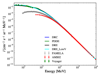
   Figure 1: Propagated proton LIS of the three baseline models DRE (black line), DRC (blue line), and PDDE (green line), plus DRELowV model (cyan line, described in Section 3.2.1) compared with data: red circles, AMS02 (Aguilar et al., 2015b); green squares, Voyager 1 (Cummings et al., 2016); grey diamonds, PAMELA (Adriani et al., 2013). Propagation and hadronic injection parameters are as in Cummings et al. (2016) for DRE and PDDE models, and as in Boschini et al. (2017b) for DRC model.

2. DRE: Also for this model we adopt the best-fit hadronic CRs injection spectra and propagation parameters from the very recent work by Cummings et al. (2016). This corresponds to the model with diffusion and reacceleration, which is statistically favored with high significance with respect to the previous plain diffusion model ($PDDE$). More details on the modeling are described above and in Cummings et al. (2016). We run GALPROP with these parameters, and the derived proton spectrum is shown in Fig. 1. Spectra of additional hadrons can be found in the original paper.

3. DRC: More recently, CR propagation models in the Galaxy were combined with propagation models in the heliosphere to reproduce direct measurements of CR hadrons at different modulation levels and at both polarities of the solar magnetic field (Boschini et al., 2017b). A propagation model including diffusion, reacceleration, and convection was found (Boschini et al., 2017b) to give the best agreement with proton, helium, and antiproton data by AMS-02, BESS, PAMELA and Voyager 1 from 1997 to 2015. The experimental observables included all published AMS-02 data on protons (Aguilar et al., 2015b), helium (Aguilar et al., 2015a), B/C ratio (Aguilar et al., 2016). This is the most recent model for hadrons, where hadronic CRs and propagation parameters were fitted to AMS-02 and Voyager 1 measurements. The HelMod code that computes the transport of Galactic CRs through the heliosphere down to the Earth was used. This provides a more physical treatment of the solar modulation instead of the force-field approximation. HelMod integrates the transport equation (Parker, 1958) using a Monte Carlo approach that involves stochastic differential equations. More details on HelMod are provided in Bobik et al. (2016) and Boschini et al. (2017a), while on the joint implementation of HelMod with Galprop in Boschini et al. (2017b), where a MCMC procedure was used to determine the propagation parameters.
   The best-fit CRs injection and propagation parameters from that work are used to build our model with diffusion, reacceleration and convection. We run GALPROP with these parameters, and the derived proton spectrum is shown in Fig. 1. Also here, spectra of additional hadrons can be found in the original paper.

For the three models, PDDE, DRE, DRC, the propagation parameters are summarized in Table LABEL:Table1. They are: $D_{0_{xx}}$, the normalization of the diffusion coefficient at the reference rigidity $D_{R}$; $D_{br}$, the rigidity break where the index of the rigidity can assume different values ($\delta_{1}$ and $\delta_{2}$); the Alfven velocity $v_{Alf}$; the convection velocity $v_{c}$, and its gradient $dV/dz$.

Table 1: The table shows the propagation and the proton injection parameters of the models. Injection parameters for other nuclei are as in the original works (Cummings et al., 2016; Boschini et al., 2017b) and are not repeated here. The description of each parameter can be found in the text.

Model code	DRE	DRC	PDDE	DRELowV(b)
Propagation
parameters
D0 (a) (cm2 s-1)	14.6	4.3	12.3	14.6
Dbr $(GV)$	-	-	4.8	-
$\delta_{1}$	0.327	0.395	-0.641	0.327
$\delta_{2}$	0.323	0.395	0.578	0.323
VAlf (Km s-1)	42.2	28.6	-	8.9
Vc (Km s-1)	-	12.4	-	-
dV/dz (km s-1 kpc-1)	-	10.2	-	-
Proton
injection
parameters
$\gamma_{1}$	0.65	1.69	1.18	-
$\gamma_{2}$	1.94	2.44	2.95	1.4
$\gamma_{3}$	2.47	2.28	2.22	2.47
E${}_{br_{1}}$ $(MV)$	117	700	124	-
E${}_{br_{2}}$ $(GV)$	17.9	360.0	6.5	2.7

^a D_xx=10${}^{28}\beta D_{0}(R/D_{R})^{\delta}$ cm² s^-1, with $D_{R}$=4GV for DRC model, and $D_{R}$=40GV for the other models.
The propagation halo size is 4 kpc for all the models.
^b This propagation model is described in Section 3.2.1.

Model fitting of all-electrons was not addressed in the works by Cummings et al. (2016) and Boschini et al. (2017b). In this present work we infer injection spectral parameters of primary electrons to reproduce the CR all-electron measurements by Voyager 1 and AMS-02, together with multifrequency data where possible. The resulting electron injection parameters will be given and discussed in Section 3.

2.1.3 Interstellar emission calculations

For each propagation model we generate the skymaps in the HEALpix scheme (Górski et al., 2005) for the different interstellar emission mechanisms that are IC, pion decay, bremsstrahlung, and synchrotron. This is done by using the best 3D magnetic field formulation as found in Orlando & Strong (2013) (as used in the so-called ’SUN10E’ model in that paper), and the ISRF and gas model components as in Ackermann et al. (2012). Regarding this latter component the conversion factor from CO to H₂ (X_{C O}) is assumed to be in the best-fit ranges as found in Ackermann et al. (2012) that better reproduces Fermi LAT gamma-ray data in the entire Galaxy. Specifically, for this conversion we make use of four Galactocentric rings having radii of 2, 6, 10, and 20 kpc with X_CO values of 0.5, 6, 10, and 20 $\times$ 10²⁰ cm^-2(K km s^-1)^-1. An additional ingredient for computing the interstellar emissions is the distribution of CR sources, which is based on pulsars (Lorimer et al., 2006) as in Ackermann et al. (2012). As suggested by Fermi LAT gamma-ray data (Abdo et al., 2010; Ackermann et al., 2011, 2012) and radio observations (Orlando & Strong, 2013) we assume it to have a constant profile for a Galactocentric distance larger than 10 kpc. The IC emission is calculated with the anisotropic formulation of the Klein-Nishina cross section (Moskalenko & Strong, 2000).

2.2 Observations

For this study we use CR measurements and data from radio to gamma rays as described below.

2.2.1 CR measurements

Measurements of the CR spectra are affected by solar modulation below a few ten GeV only, and until recently no CR data free from this effect were available below those energies. Since August 2012 Voyager 1 observes a steady flux of Galactic CRs down to 3 MeV/nucleon for nuclei and to 2.7 MeV for all-electrons, which is independent on the solar activity. This is a strong indication of the instruments measuring the true LIS (Cummings et al., 2016). We use Voyager 1 all-electron measurements (Cummings et al., 2016) together with the precise AMS-02 electron (Aguilar et al., 2014) and positron (Accardo et al., 2014) data. PAMELA electron measurements (Adriani et al., 2015) are also used for additional constraints.

2.2.2 Radio surveys

Building upon the successful approach of Strong et al. (2011) we make use of those ground-based radio surveys at frequencies between 45 MHz and 1420 MHz, which display a nearly complete sky coverage ($>$80 per cent) in the region of interest. In the following we describe the single maps in more detail. At lowest frequencies the 45 MHz North map (Maeda et al., 1999) and the South map (Alvarez et al., 1997) were combined to obtain an all-sky map by Guzmán et al. (2011) with an offset of 500K. At somewhat higher frequencies, we adapt the 150 MHz map from the Parkes-Jodrell Bank all-sky survey (Landecker & Wielebinski, 1970). At 408 MHz the Haslam map (Haslam et al., 1981, 1982) as reprocessed by Remazeilles et al. (2015) is used in this work. We corrected this map by subtracting an offset of 8.9 K following the recent studies by Wehus et al. (2017), Planck Collaboration et al. (2016a) and Planck Collaboration et al. (2016), which are found to be in agreement with our previous work (Orlando & Strong, 2013). The 408 MHz map is the only full-sky radio map with limited contamination from thermal emission. In addition, instrumental effects and sources have been accurately removed. These properties make this map an ideal tracer of the synchrotron radio emission from the Galaxy. At higher frequencies the combined 1420 MHz North map from Reich (1982) and South map from Reich et al. (2001) are corrected for an offset of 3.28 K as computed in the very recent work by Wehus et al. (2017). This value is in agreement with an exhaustive work by Fornengo et al. (2014). Offsets represent the sum of any instrumental and data processing offsets, as well as any Galactic or extra-Galactic components that are spectrally uniform over the full sky, including the CMB contribution.
To spectrally compare our propagation models with data we use the region of intermediate latitudes (i.e. 10^∘$<|b|<$20^∘) because this includes mostly the local emission within $\sim$ 1 kpc around the Sun and, hence, it encodes the CR LIS. Moreover, the region of intermediate latitudes is optimal because the synchrotron emission is the least contaminated: for $|b|<$20^∘ offsets are not crucial even though we account for them, while for $|b|>$10^∘ free-free absorption and emission are less than a few percent. However, we remove this small contamination of the free-free emission by using the free-free spatial template released by the Planck Collaboration and by following the spectral formulation for the free-free emission as in Planck Collaboration et al. (2016a). We also account for the small contribution of the absorption using the implementation explained in detail in Orlando & Strong (2013).

2.2.3 Microwave maps

To study the synchrotron component we use the accurate four-year Planck synchrotron temperature map (Planck Collaboration et al., 2016a) released by the Planck Collaboration. For an independent comparison we use also the nine-year Wilkinson Microwave Anisotropy Probe (WMAP) synchrotron maps (Bennett et al., 2013) at 23, 33, 41, 61 and 94 GHz obtained with the Maximum Entropy Method. While Planck provides the today’s most accurate information on the synchrotron emission at microwave frequencies, the derivation of its intensity map is model dependent (Planck Collaboration et al., 2016a). The derivation and relevance of Planck and WMAP maps will be discussed in Section 3.5.
Following the approach adopted for the radio surveys explained in Section 2.2.2, also the microwave synchrotron maps are used at intermediate latitudes (i.e. 10^∘$<|b|<$20^∘), excluding the Galactic plane where the contamination by free-free emission and anomalous microwave emission is important. In turn, this allows us comparing synchrotron spectra with models in a frequency range from a few tens of MHz to a few tens of GHz.

2.2.4 Gamma rays

The spectrum of the gamma-ray emission with its interstellar components (pion decay, bremsstrahlung and inverse Compton) encodes the spectra of CRs in the Galaxy. A detailed study of the interstellar emission from the whole Galaxy was performed on a grid of 128 propagation models (Ackermann et al., 2012) using the Fermi-LAT data. Even though all models provide a good agreement with data, no best model was found. That study extensively investigated many GALPROP CR propagation models accounting for uncertainties in the models, such as ISRF, gas distribution, HI spin temperature, propagation halo size, and CR source distribution. However, it investigated propagation models with reacceleration only, which are challenged by synchrotron data (Strong et al., 2011; Jaffe et al., 2011). Here we test how different propagation models (i.e. DRE with reaccelereation, PDDE plain diffusion, and DRC with convection) spectrally compare with gamma-ray data. As a first step we use Fermi LAT gamma-ray spectra obtained in the study of Ackermann et al. (2012) for intermediate latitudes (i.e. 10^∘$<|b|<$20^∘). For the purpose of comparisons, models are treated like data, i.e. integrated and averaged in the same sky region.
In a second step, we use a specific dataset: the local HI gamma-ray emissivity. This directly encodes the spectra of CR LIS. The derivation of the emissivity requires a careful approach. Such an approach has been followed in a recent work (Casandjian, 2015). In it the HI emissivity for the mid-latitude (10^∘$<|b|<$70^∘) band, which is considered local, is derived by using Fermi LAT P7 reprocessed data having energies between 50 MeV and 50 GeV that were taken in 4 years of observations, based on the extensive analysis in Acero et al. (2016). This work (Casandjian, 2015) carefully accounts for the Fermi LAT energy dispersion, which impacts the spectrum below a few hundred MeV. It accounts also for large-scale structures such as the North Polar Spur (Haslam et al., 1981), the so-called Fermi bubbles (Su et al., 2010; Dobler et al., 2010; Ackermann et al., 2014), and the Earth’s Limb emission. In the derivation of the local HI emissivity and its error bands three major sources of systematic errors are properly accounted for: the HI spin temperature, the modeling of the IC, and the absolute determination of the Fermi LAT effective area (Casandjian, 2015). This recent derived local HI emissivity is used in our model comparisons.
As the last step, we look at the Galactic centre region by using Fermi LAT spectra obtained with 6.5 yeas of observations that were very recently published in Ackermann et al. (2017). In this work, the original data are in flux units that we have converted in intensity. For the purpose of comparisons, models are treated like data, i.e. integrated and averaged in the same sky region, and masking out the most luminous sources as done to the original data. These data are very suitable for qualitatively model comparisons of the 10^∘ region around the Galactic centre. Due to the complexity in this region we focus on the interstellar emission produced by the above propagation models neglecting the other components (i.e. isotropic, faint sources, solar and lunar, etc.), as reported in Section 3.4.

2.2.5 X-rays and soft gamma rays

At X-ray and soft gamma-ray energies data are taken by the INTErnational Gamma-Ray Astrophysics Laboratory (INTEGRAL) mission (Winkler et al., 2003) with its coded-mask telescope SPI, the SPectrometer for INTEGRAL(Vedrenne et al., 2003). In a detailed study by Bouchet et al. (2011), spectral data of the Galactic diffuse emission are provided for energies between $\sim$80 keV and $\sim$2 MeV. Data were taken for a very long integration time ranging from year 2003 to 2009 for a total exposure of $\sim$10⁸s on the sky region $|b|<$15^∘ and 330^∘$<l<$ 30^∘. For the same sky region intensity data at somewhat higher energies between 1–30 MeV are provided by Strong et al. (1999) from the Imaging Compton Telescope (COMPTEL) instrument (Schoenfelder et al., 1993) on board of the Compton Gamma-Ray Observatory. Adopting the energy ranges from Strong et al. (1999), maps are used in three energy bands: 1–3 MeV, 3–10 MeV, and 10–30 MeV.
SPI and COMPTEL data were both cleaned by subtracting the sources (Strong et al., 1999; Bouchet et al., 2011). For the limited sensitivity of those instruments at hard X-rays and MeV energy ranges, data in the inner Galaxy region, where the diffuse emission is maximum, are very suitable for model comparisons.

3 Results

This section presents results from the comparison of the GALPROP propagation models with CR measurements and multi-wavelength data.

3.1 Baseline models

For the three baseline models (DRE, DRC, PDDE) the propagation parameters for primary electrons are fixed to the values found for the hadronic propagation parameters. The primary electron spectra parameters (injection spectral indexes and breaks) instead are inferred so that the all-electrons reproduce, after propagation, the precise data by AMS-02 above a few tens GeV and to reproduce the very recently measured data by Voyager 1 below 30 MeV. At the same time, primary electrons are inferred also to reproduce at best the synchrotron data (i.e. radio and microwave surveys), as discussed in the next paragraph. PAMELA data data are used as an additional constraint: the LIS can not be lower than the direct measurements (being taken during solar minimum PAMELA measurements are higher than AMS-02 measurements). Positrons that contribute to the well-known ’positron excess’ above 10 GeV are considered to originate from local sources (e.g. Mertsch & Sarkar, 2014; Di Mauro et al., 2016; Della Torre et al., 2015). These sources are supposed to produce also the same amount of electrons. The contribution of these local electrons and positrons to the interstellar emission from radio to gamma energies is negligible.
Injection electron parameters are reported in Table LABEL:Table2, with $\gamma_{1}$, $\gamma_{2}$, $\gamma_{3}$ spectral indexes, and $E_{br_{1}}$, $E_{br_{2}}$ energy breaks.

Table 2: The table shows the electron injection parameters of the models. The description of each parameter can be found in the text.

Model code	DRE	DRC	PDDE	DRELowVa
$\gamma_{1}$	2.90	2.75	2.01	2.20
$\gamma_{2}$	0.80	0.65	2.55	1.70
$\gamma_{3}$	2.65	2.62	-	2.68
E${}_{br_{1}}$ $(MV)$	320	400	65	170
E${}_{br_{2}}$ $(GV)$	6.3	4.0	-	4.5

^a This propagation model is described in Section 3.2.1.

For the three propagation models (DRE, DRC, PDDE) Figure 2 shows the comparison of the propagated all-electron LIS (solid lines), along with their distinct components of electrons (dashed lines) and secondary positrons (dotted lines), with the direct CR measurements (squares for Voyager 1, dots for AMS-02 electrons, crosses for AMS-02 positrons, dashes for PAMELA electrons). The three baseline models produce three different all-electron LIS densities in the range $\sim$(10²–10⁴) MeV. In this range the low all-electron density of the PDDE model (red line in Figure 2) is due to the break of the diffusion coefficient, while the injection spectrum is the same downwards to a few tens of MeV. Only below a few tens of MeV a break in the injection spectrum is necessary to avoid overestimating Voyager 1 data. On the other hand, the DRC (black line in Figure 2) and the DRE (green line in Figure 2) models require two breaks in the primary electron injection spectra to reproduce Voyager 1 data. We can summarize by saying that models without breaks in the injection spectrum of primary electrons at low energies can not reproduce the Voyager 1 data. It is worth noting that the contribution of secondary positrons in the range $\sim$(10²–10⁴) MeV for the models encoding reacceleration (i.e. DRC, DRE) is a factor of ten larger compared to the PDDE model. While the very similar proton spectrum among the three models can not account for this difference, reacceleration processes can.

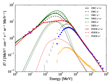
Figure 2: Propagated interstellar spectra of the three baseline models DRE (green line), DRC (black line), and PDDE (red line) for positrons (dotted lines), electrons only (dashed lines), and all-electrons (solid lines) compared with data: orange crosses: AMS-02 positrons (Aguilar et al., 2014); blue points: AMS-02 electrons (Aguilar et al., 2014); grey dashes: PAMELA electrons (Adriani et al., 2015); magenta squares: Voyager 1 all-electrons (Cummings et al., 2016).

We report here on the comparison of the calculated synchrotron spectra to the synchrotron data. As previously stated the primary electrons were tuned so that the all-electrons reproduce at best not only the direct CR measurements but also the synchrotron data for the energy range where the CR direct measurements are affected by solar modulation (i.e. $\sim$(10²–10⁴) MeV). To constrain the CR all-electrons with synchrotron data, we use the best-fit normalization of the magnetic field intensity found by spatially fitting the calculated synchrotron template to the observed 408 MHz map, after subtracting the free-free emission component and the offsets, as successfully performed in our previous work (Orlando & Strong, 2013). In Figure 3 we display the resulting synchrotron spectra of the three baseline models (DRE solid line, DRC dotted line, PDDE dashed line) using the all-electrons as in Figure 2. We compare the calculated spectra to the synchrotron emission by radio surveys and by the Planck synchrotron map integrated at intermediate latitudes. While Planck provides the today’s most accurate information on the synchrotron emission at microwave frequencies, WMAP maps are used as upper limits (see discussion on Planck and WMAP uncertainties in Section 3.5). Figure 3 shows that the synchrotron spectrum of the PDDE model performs best in the entire frequency range compared to the DRE and DRC models that overestimate the observations at frequencies below 408 MHz. The overestimation is due to the larger density of the all-electron LIS at $\sim$(10²–10⁴) MeV. This enhancement is due to strong reacceleration processes (with Alfven velocity around 30 – 40 km/s) responsible to contribute to secondary CRs. This is in agreement with our previous findings (Strong et al., 2011). The same significant amount of secondaries prevents from tuning the primary electron spectrum of the DRE and DRC models in such a way to reproduce the synchrotron intensity at $\sim$(10 – 400) MHz. At these frequencies the eye-catching gap between the DRE/DRC models and the PDDE model can be seen in Figure 3. To further investigate this difference we make use of the following additional approach. To avoid assumptions on primary electrons, we derive these by subtracting the secondaries, calculated with GALPROP for the three baseline models (DRE, DRC, PDDE), from the all-electron LIS that fits both synchrotron observations and CR measurements. After the subtraction we are left with the spectrum of primary electrons only, which can be compared to the electron direct measurements by PAMELA and AMS-02. As a result, the primary electron spectrum obtained for DRE and DRC models below a few GeV are either negative or null. This means that the spectrum of secondaries for the DRE and DRC model is larger or equal to the all-electron LIS that reproduces the synchrotron data. This leaves no space for a meaningful primary electron spectrum of the DRE and DRC models. Instead, for the PDDE model, the derived spectrum of primary electrons is in agreement with CR measurements. We can conclude that the two independent approaches (i.e. the latter approach without assumptions on the primary electron spectrum, and the previous approach with the tuning of it) lead to the same result: propagation models that produce significant amount of secondaries or that have a large all-electron intensity in the range $\sim$(10²–10⁴) MeV are difficult to reconcile with synchrotron data.
The values of the spectral intensity of all-electron LIS for our best model PDDE is reported in Appendix (Table 5).

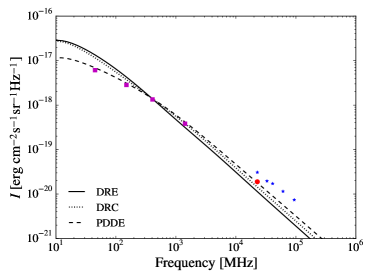
Figure 3: Synchrotron spectra for intermediate latitudes (10^∘$<|$b$|<$20^∘) of the three baseline models DRE (solid lines), DRC (dotted line), and PDDE (dashed line) compared with data: radio surveys (magenta squares) (described in Section 3.2), Planck synchrotron map (red point) (Planck Collaboration et al., 2016a), and WMAP (blue stars) (Bennett et al., 2013).

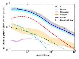
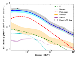
Figure 4: Calculated gamma-ray spectral intensity of the three baseline models, left to right, DRE, DRC, and PDDE. Data are Fermi LAT spectra at intermediate regions (10^∘ $<$|b|$<$20^∘, all longitudes) from Ackermann et al. (2012). Models are: pion decay (red dashed line), IC (green dash-dotted line), bremsstrahlung (cyan dotted line). Data include statistical errors (grey area) and systematic errors (black bars). Spectra for sources (magenta region) and isotropic component (yellow region) are taken from Ackermann et al. (2012), for the most extreme cases reported there. Uncertainty of 30 per cent is added to the isotropic spectrum, following the study in Ackermann et al. (2015) based on various foreground models. Interstellar model components are not fitted to data.

Gamma-ray data provide an additional source of information on the all-electron and proton spectrum. While in our previous work (Ackermann et al., 2012) only reacceleration models (similar to our DRE model) were studied, here we spectrally test the different propagation models (DRE, DRC, PDDE) with gamma-ray data. Hence, we calculate the gamma-ray emission expected from the three propagation models (DRE, DRC, PDDE) at intermediate latitudes. Figure 4 shows the comparison of these predictions with Fermi LAT data for the intermediate latitudes as published in Ackermann et al. (2012). Spectra for detected gamma-ray sources and for the isotropic emission are taken from Ackermann et al. (2012), for the most extreme cases reported there. An uncertainty of 30 per cent is added to the isotropic spectrum, following the study in Ackermann et al. (2015) based on various foreground models. Below a few hundred MeV, DRE and DRC models produce higher gamma-ray emission than PDDE model due to the enhanced all-electron density, which in turn increases the bremsstrahlung emission. However, all the models are within the Fermi LAT systematic uncertainties. Hence, in a first approximation, with the data used here, also plain diffusion models, such as our PDDE model, reproduce gamma-ray data as well as reacceleration models. However, in general, analyses of the gamma-ray data in various regions of the Galaxy suffer from large uncertainties mainly given by the ISRF and the gas density (e.g. Ackermann et al., 2012, 2015; Ajello et al., 2016; Acero et al., 2016).

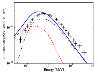
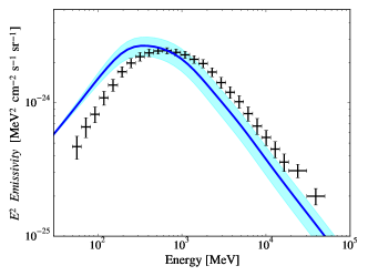
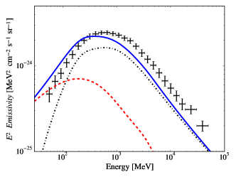
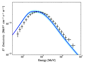
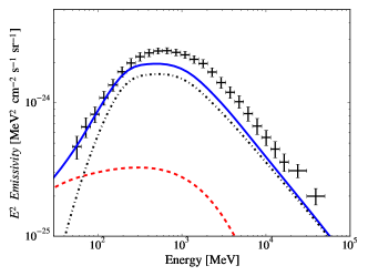
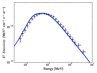
Figure 5: Local gamma-ray emissivity of the three baseline models, top to bottom, DRE, DRC, and PDDE compared with Fermi LAT local HI emissivity (Casandjian, 2015). Left: Calculated bremsstrahlung components (red dashed lines), pion-decay components (blue dashed-dotted lines), and their sum (blue solid lines) are shown. Right: the sum (blue solid lines) of the calculated bremsstrahlung and the fitted pion-decay components, and the 1-$\sigma$ error (cyan region) in the fitted parameter are shown. Fitted parameters for the pion decay components, errors, and chi-squares of the fit are reported in Table LABEL:Table3 (normalization for the entire energy band).

Table 3: The table shows the best-fit values of the pion decay component to the gamma-ray emissivity.

Model	Normalization	chi-square	Normalization
	(entire energy band)		(> 1 GeV)
DRE	0.95 $\pm$ 0.26	10.5	1.38 $\pm$ 0.07
DRC	1.20 $\pm$ 0.15	4.2	1.45 $\pm$ 0.03
PDDE	1.30 $\pm$ 0.05	1.2	1.40 $\pm$ 0.05
DRELowVa	1.35 $\pm$ 0.05	0.6	1.40 $\pm$ 0.05

^a This propagation model is described in Section 3.2.1.

A precise way to obtain information about CR spectra and density in various places in the Galaxy is to study the emissivity per H atom that reflects the CR spectra free from uncertainties on the ISRF and gas distributions (e.g Abdo et al., 2010; Ackermann et al., 2011; Tibaldo et al., 2015). The HI emissivity includes the bremsstrahlung and pion decay components. A recent study was performed by Casandjian (2015), which derived the local HI emissivity. We examine our baseline models by comparing the calculated gamma-ray emissivity at the location of $\sim$1 kpc around the sun to the local HI emissivity data from Fermi LAT (Casandjian, 2015). To facilitate the comparison between data and models, in Figure 5 we display from top to bottom the three baseline models DRE, DRC, and PDDE. Plots on the left show the calculated components compared to the data, while plots on the right show the result of fitting the components to the data. In all of the three plots on the left, Fermi LAT data (Casandjian, 2015) are black crosses, the sum of the calculated components are solid lines, their bremsstrahlung component is dotted, and their pion-decay component is dashed. For the first two plots on the left is it clear that the DRE and DRC models (blue solid lines) overestimate the data below several hundred MeV (black crosses). More strikingly, even their bremsstrahlung component (dotted line) alone overestimates the data below 100 MeV. This finding strongly disfavors the DRE and the DRC models. Instead the PDDE model (bottom plot in Figure 5) reproduces the data very well below a few hundreds of MeV. This finding, that models with relatively low all-electron intensity below a few GeV reproduce gamma-ray data, reinforces the previous results where the same low all-electron intensity reproduces the radio observations. Above a few hundreds of MeV, for all the models the predictions of the local emissivity fail to reproduce the Fermi LAT observations (left plots in the same figure). To quantify this difference between data and models, Table LABEL:Table3 reports the best-fit scaling factors of the pion decay components for the three models (DRE, DRC, PDDE, plus one model discussed later). The fit is performed by freezing the normalization of the bremsstrahlung component and leaving the normalization of the pion decay component free to vary. The chi-square values reported in Table LABEL:Table3 are significantly better for the PDDE model over the DRE and DRC models, which poorly fit the data (see also the right plots on Figure 5 especially below a few hundred MeV). DRE and DRC models still overestimate the data below a few hundred MeV, thereby being disfavored by data. Regarding the PDDE model, to match the measured data the numerical value suggests that the pion decay requires an increase of at least 30 per cent. Table LABEL:Table3 reports also the best-fit scaling factors of the pion decay component performed above 1 GeV only, where the contribution of the bremsstrahlung component is not significant. The best-fit scaling factors are around 1.3 – 1.4 for all the models. Beside preferring the PDDE model, this comparison of the calculated emissivity with the observed emissivity suggests that the direct CR measurements do not represent the average spectrum in the local region within $\sim$ 1 kpc probed by the observed local gamma-ray emissivity, even if solar modulation is taken into account. Hence, we derive the proton spectrum that best reproduces the emissivity, based on the best-fit value reported in Table LABEL:Table3 for PDDE model (for the entire energy range). Our resulting proton LIS (red solid line) is compared to AMS-02 proton measurements (black points) in Figure 6. The red region includes 10 per cent uncertainty on the cross sections (Casandjian, 2015) and the uncertainty in the fit parameter estimation (Table LABEL:Table3). The discrepancy between our LIS based on the emissivity and the CR measurements from AMS-02 is evident even beyond the influence of the solar modulation. Above a few GeV our normalized proton spectrum is general agreement with a recent work by Strong (2015) on behalf of the Fermi LAT collaboration and with an earlier work by Dermer et al. (2013), in which the proton LIS has been obtained from the local gamma-ray emissivity in a model independent approach. Their complementary approach independently supports our results. However, the discrepancy data-model in Strong (2015) was not found to be as strongly significant as we instead find now because in that work the proton spectrum derived from the emissivity was compared to PAMELA data, which have larger uncertainties than AMS-02 (more than 20 per cent uncertainties in PAMELA data with respect to 5 per cent uncertainty maximum in AMS-02). This most likely prevented Strong (2015) from drawing definitive conclusions upon. The same figure also shows the best-fit LIS from Strong (2015) and Casandjian (2015) for comparison (uncertainties are not plotted), supporting our conclusion that latest precise CR proton measurements do not resemble the LIS within $\sim$1 kpc from the sun, even after accounting for solar modulation. The differences among the proton spectra obtained by Strong (2015), by Casandjian (2015) and by the present work are most likely due to the pion production cross sections and to the all-electron spectrum used. Indeed, hadronic cross sections are still affected by significant uncertainties especially for CRs and target nuclei with atomic number $Z>1$, (e.g. Kamae et al., 2006) For heavier nuclei the calculated emissivity (Casandjian, 2015) have a nuclear enhancement factor of 1.8 for proton-proton interactions as found by Mori (2009), while we have 1.5 that would account for a few per cent difference in the calculation of the emissivity (Casandjian, 2015). The best-fit proton spectrum by Strong (2015), obtained with a sophisticated Bayesian approach with MultiNest, is in agreement with our spectrum down to $\sim$3 GeV. The discrepancy at lower energy is mostly due to differences in the all-electron spectrum used to calculate the bremsstrahlung emissivity component. This bremsstrahlung emissivity component is well constrained by direct CR measurements and synchrotron emission in our present work.
Similarly to our result on the enhanced proton LIS based on gamma-ray data, an earlier work by Ackermann et al. (2015), which used a different approach still based on propagation models, found the need of increasing the calculated pion-decay emission component of 50 – 70 per cent at high energies in order to fit Fermi LAT gamma-ray data at latitudes above 20^∘ up to 500 GeV. However, the main focus of that work was related to obtain the extragalactic background emission, hence the discrepancy between interstellar models and data was not further investigated.
The spectral intensity of the proton spectrum for our baseline best model PDDE is reported in Table 2 in Appendix, together with the proton spectrum that fits the emissivity (Figure 6).

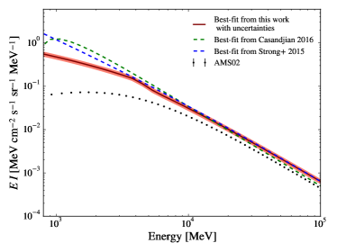
Figure 6: Best-fit proton LIS from this work (red solid line) based on emissivity observations (Casandjian, 2015) including uncertainties (red region) compared with AMS-02 proton data (Aguilar et al., 2015b) (black points). The calculated spectrum is obtained by normalizing the PDDE proton spectrum with the best-fit value of 1.3 (see Table LABEL:Table3, normalization for the entire energy band). Uncertainties include 1-$\sigma$ error in the normalization and 10 per cent uncertainties in the pion cross section (Casandjian, 2015). Best-fit LIS from Strong (2015) (blue dashed line) and Casandjian (2015) (green dashed line) are also shown for comparison (uncertainties are not plotted).

3.2 Exploring modifications to the baseline models

In this section we test a modification to one of our models (Section 3.2.1), and we test a different scenario (Section 3.2.2).

3.2.1 DRELowV model

In the effort to find propagation models with reacceleration working both with CR all-electron measurements and with the synchrotron emission we test a modified DRE model. The modification is based on a recent work (Jóhannesson et al., 2016) where we perform a Bayesian search of the main GALPROP parameters, using the MultiNest nested sampling algorithm, augmented by the BAMBI neural network machine learning package. More specifically, in that work we found that the propagation parameters that best-fit low-mass isotope data (p, p^-, and He) are significantly different from those that fit light elements (Be, B, C, N, and O), including the B/C and ¹⁰Be/⁹Be, secondary-to-primary ratios normally used to calibrate propagation parameters. This suggests that each set of species is probing a different interstellar medium, and that the standard approach of calibrating propagation parameters for all the species using B/C may lead to incorrect results (as previously suggested by the work in Genolini et al. (2015)). Based on this finding, here we explore a different propagation model that we call DRELowV, which represents an attempt to find a reacceleration propagation model that can reproduce CR measurements, and also the synchrotron spectrum as good as the PDDE model. In more detail, starting from the DRE baseline model, we make some simple modifications to the model parameters in order to reduce the amount of secondary positrons in the range $\sim$(10²–10⁴) MeV, and to consequently better reproduce all the data. In particular, we decrease the Alfven velocity of the DRE model to 8.9 km/s for protons and helium only, based on results from Jóhannesson et al. (2016) previously discussed. We modify the proton spectrum to be similar to the spectra of the baseline models, keeping all the other propagation parameters unchanged. The resulting proton spectrum is shown on Figure 1. The spectrum of the light elements are unchanged with respect to the original models, hence, they are not reported here. Spectra and parameters of the light elements can be found in the original paper, where elements up to Si from ACE-CRIS, HEAO3, PAMELA, and CREAM were fitted. Then, following the procedure used for the baseline models, here we adjust the electron injection spectral indexes and breaks in such a way that the density of all-electrons in the range $\sim$GeV is similar to the PDDE model. This is now possible because of the lower density of secondaries produced by the decreased Alfven velocity with respect to DRE model. Model parameters are summarized in Table LABEL:Table1 and Table LABEL:Table2. The resulting DRELowV model requires at least two breaks in the primary injection electron spectrum below a few GeV in order to reproduce the AMS-02 and Voyager 1 data. Figure 7 shows the propagated interstellar all-electron spectra for DRELowV model against data. Compared to Figure 2 we find that the density of positrons at $\sim$GeV for this model is a factor of 2.5 lower than the baseline DRE and DRC models, and it is similar to the PDDE model.

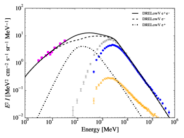
Figure 7: Propagated interstellar spectra of the DRELowV model for positrons (dashed-dotted line), electrons only (dashed line), and all-electrons (solid line) compared with data as described in Figure 2.

The synchrotron spectrum is calculated and is shown in Figure 8. We find that the spectral data are quite well reproduced in the whole frequency range, as for the case of PDDE model. As a consequence this propagation model and the resulting LIS are a good representation of the spectrum that produces the synchrotron emission, as found for PDDE model. This suggests that the contribution of secondaries and primary electrons is now well constrained, meaning that it is possible to find a propagation model with reacceleration (with significantly reduced reacceleration compared to the usually assumed for protons) consistent also with radio synchrotron data.

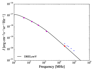
Figure 8: Synchrotron spectrum for intermediate latitudes (10^∘$<|b|<$20^∘) of the DRELowV model compared with data as in Figure 3.

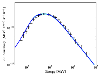
Figure 9: Local gamma-ray emissivity of DRELowV model compared with Fermi LAT local HI emissivity (Casandjian, 2015). Top: Calculated bremsstrahlung component (red dashed lines), pion-decay component (blue dashed-dotted lines), and their sum (blue lines) are shown. Bottom: the sum (blue lines) of the calculated bremsstrahlung and the fitted pion-decay component, and the 1-$\sigma$ error (cyan region) in the fitted parameter are shown. The fitted parameter for the pion decay component, errors, and chi-squares of the fit are reported in Table LABEL:Table3.

Following the same procedure as used for the baseline models, we calculate the local gamma-ray emissivity for DRELowV model and we compare it with data. Figure 9 shows that, similarly to what happens to the PDDE model, a very good agreement is visible for the DRELowV model below a few hundred MeV (top plot). This confirms the preference of models with low all-electron density at the $\sim$GeV range. At higher energies, instead, the predictions of the local gamma-ray emissivity are still $\sim$ 30 – 40 per cent lower than the Fermi LAT observations, as also found for the baseline models. This suggests that proton CR measurements are not resembling the LIS within $\sim$1 kpc even if accounting for solar modulation, as found in Section 3.1. Figure 9 (bottom plot) shows the normalized emissivity, while Table LABEL:Table3 summarizes the best-fit results for this model, leading to scaling factors very similar to the PDDE model. This is not surprising since the all-electron LIS and the proton LIS of the two models are alike.
Note that in principle modifications to the DRC model as performed for the DRELowV model could be possible. However repeating the procedure as in Jóhannesson et al. (2016) to obtain a fully Bayesian parameter estimation for the DRC model including convection is beyond the present effort.

3.2.2 The electron LIS at high energies

In the following we aim at verifying whether our initial assumption on the ’positron excess’ affects the results. We assume here that the high-energy positron spectrum (that includes the ’positron excess’) is produced by injection and propagation and it is not peculiar to our position in the Galaxy and our proximity to an electron-positron source. In other words we assume the distribution of the Galactic sources producing positrons at high energies to be the same compared to the distribution of the sources of primary electrons. Once computed the synchrotron emission we find that this modification does not effect the intensity in radio and microwaves, i.e. radio and microwaves are not sensitive to the energy range of the ’positron excess’. In addition, we also find that this modification does not effect the computed gamma-ray emissivity either, because electrons and positrons are too energetic to contribute to the emission. Consequently, neither radio/microwaves nor the gamma-ray emissivity is affected by positrons at those energies, which could instead contribute to the gamma-ray emission at high energies via IC above a few GeV.

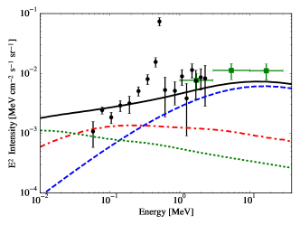
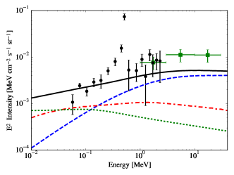
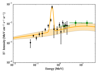
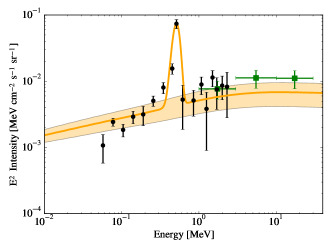
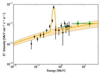
Figure 10: X-ray and soft gamma-ray spectra of the models, left to right, DRE, DRC, PDDE, and DRELowV. Top two rows show the three IC components as modeled: on the CMB (green dotted line), on the diffuse IR (red, dash-dotted line), and on the diffuse optical (blue dashed line), along with their sum (black solid line). Bottom two rows show the sum of the components after the fit (orange line) with one sigma error region (orange region). Data are from Bouchet et al. (2011) for the inner Galaxy $|b|<$15^∘ and $|l|<$30^∘ from SPI (black points) and from COMPTEL (green points) with respective error bars. Fit results are reported in Table LABEL:Table4.

3.3 X-rays and soft gamma rays from the inner Galaxy

After studying the spectra of CRs in the local interstellar medium, we use our resulting models, DRE, DRC, PDDE, and DRELowV, to compute the emission from the inner Galaxy observed in the range 0.1 - 30 MeV, following the work in Bouchet et al. (2011) and in Porter et al. (2008), to see how they compare to X-rays and soft gamma-ray data. Our sky region of interest is $|b|<$15^∘ and 330^∘$<l<$ 30^∘. In this energy range IC emission is the only CR-induced interstellar component. We separately calculate the contributions to the IC intensity by optical, infrared (IR), and CMB photons. Figure 10 shows the spectral component contributions to the diffuse IC emission for all the models (two upper rows of the figure, left to right: DRE, DRC, PDDE, and DRELowV) compared to SPI and COMPTEL spectral data, as published by Bouchet et al. (2011). The three IC components (by CMB, by optical, and by IR photons) are visualized, together with their summed emission. To account for uncertainties in the ISRF we fit the normalization of the IC components to the data with the following method. Because the optical and IR components are physically related, a common scaling parameter for both is used following the work in Ackermann et al. (2012) by the Fermi LAT Collaboration. The CMB component is instead fixed since the CMB is known. A gaussian emission line at 511 keV for the electron-positron annihilation is also added. The best-fit values for all the models are collected in Table LABEL:Table4, while the resulting fitted IC emission is shown in Figure 10 (two bottom rows, left to right: DRE, DRC, PDDE, and DRELowV model). We find that while our preferred PDDE and PDDELowV models require a scaling factor of $\sim$3 in the optical and IR components in order to reproduce the data, for the DRE model the spectral shape and intensity of the diffuse IC emission matches reasonably well the data. Overall, the DRE and the DRC models reproduce the intensity of the data by SPI and by COMPTEL better than the PDDE and the DRELowV models. Their higher IC intensity with respect to PDDE and DRELowV models is due to the enhanced all-electron spectrum of those models in the $\sim$(10²–10⁴) MeV range. This is reflected in the best-fit scaling factors found to be $\sim$1 and $\sim$1.3 for DRE and DRC models respectively, as reported in Table LABEL:Table4. In general we find that models with the all-electron LIS that fit the local synchrotron emission and the local emissivity (PDDE and DRELowV) underestimate the X-ray emission in the inner Galaxy. Instead, a significant contribution from secondary positrons and electrons (as in DRE and DRC models) reproduces observations by SPI and COMPTEL of the inner Galaxy without the need of substantially enhancing the ISRF.

Table 4: Best-fit values of the IR and optical component of the IC emission derived from comparison of X-ray and soft-gamma observations by INTEGRAL/SPI and COMPTEL.

Model	IR/Optical normalization	chi-square
DRE	1.05 $\pm$ 0.44	2.92
DRC	1.35 $\pm$ 0.55	2.76
PDDE	2.98 $\pm$ 1.13	2.42
DRELowV	2.95 $\pm$ 1.11	2.37

3.4 Gamma rays from the Galactic centre

Over the last years the Galactic centre has become a region of particular interest to the astrophysical community. Especially at gamma-ray energies, the properties of this sky region might encode possible discoveries (e.g. Abazajian et al., 2014; Calore et al., 2015; Carlson et al., 2016; Linden et al., 2016; Ajello et al., 2016; Ackermann et al., 2017). Therefore, any effort in modeling the emission in this region is important.
Studies in this region often fit the interstellar model components (IC, pion, and bremsstrahlung) to data in bin-by-bin of energies. Being fitted bin-by-bin the information of the CR spectra is lost because each bin is independently adjusted together with other components (i.e. detected sources, isotropic emission, solar and lunar emission). Our approach is instead to directly compare our propagation model (DRE, DRC, PDDE, DRELowV) with Fermi LAT data with no spectral adjustments, and no fit to data. This is useful for illustration and for investigating whether present observations in this region allow for challenging some models without performing a dedicated analysis that would account for all the emission components in this difficult region. In fact, if the sum of the components (pion, bremsstrahlung, and IC) of one of our propagation models overestimates the data, it means that this model needs more attention. Moreover, while we discuss the comparison of interstellar models with data, we do not draw any new final conclusion by looking at this region alone, which would need a dedicated work. We compare our propagation models with the Fermi LAT spectral data over an area of 10^∘ radius around the Galactic centre taken from a very recent study by Ackermann et al. (2017). The comparison of models with data is shown in Figure 11, where each plot represents one model at a time (top to bottom, left to right DRE, DRC, PDDE, and DRELowV). We plot the gamma-ray intensities due to the bremsstrahlung (cyan solid lines), the IC (green solid lines), the pion-decay (red solid lines), and their sum (blue solid lines) for the propagation models that reproduce CR measurements. For DRE model at energies below 1 GeV our computed total (sum of bremsstrahlung, pion decay, and IC) interstellar emission alone (blue solid lines) over-predicts the Fermi LAT data (black points). The summed component for the DRC model is accepted by the data, if no other components (e.g. additional sources below $\sim$1 GeV ) are included. While baseline DRE and DRC models may be challenged by gamma-ray data in this region, the PDDE and DRELowV models (two plots in second row of Figure 11, blue solid lines) provide a better spectral representation of the Fermi LAT data below 1 GeV (blue solid lines). Being the pion decay emission produced by similar hadronic CR spectra for all the models, the major contribution to this difference among the models is given by the bremsstrahlung component, due to the different electrons and positrons. In addition, for all the models, the resulting components with normalized ISRF as found to fit the SPI and COMPTEL data in the inner Galaxy and reported in Table LABEL:Table4 are also plotted (blue dotted lines). Moreover, models with proton spectra scaled with the best-fit normalization in Table LABEL:Table3 (for the entire energy band), which are based on the local gamma-ray emissivity data, are shown for PDDE and DRELowV models (blue dashed lines, with blue-grey shaded region). The plots shows that PDDE and DRELowV models with enhanced ISRF and proton spectrum may be challenged as well below $\sim$ 1 GeV once other components (i.e. isotropic, faint sources, solar and lunar emission) are included. In fact, for the PDDE and DRELowV models, an increase of the ISRF (blue dotted line) would imply also an enhancement of the IC emission below a few GeV. The need for an increase of the IC emission component in the Galactic centre region was claimed in a recent study by Ajello et al. (2016), but the degeneracy between ISRF and electrons was not solved. However, in that analysis energies below 1 GeV were not included. By extending to energies down to 100 MeV, our comparison may suggest that an enhanced ISRF could be disfavored, favoring the alternative hypothesis of a harder electron spectrum in that region only.

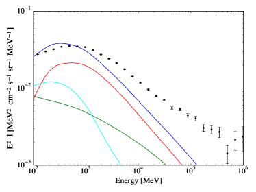
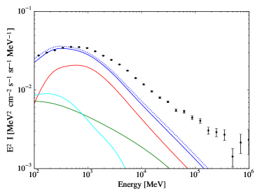
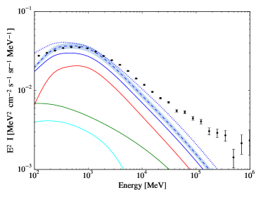
Figure 11: Gamma-ray spectral intensity for the inner Galaxy (10^∘ radius around the Galaxy centre) of the four propagation models, left to right top to bottom, DRE, DRC, PDDE, and DRELowV. Data (black points) are Fermi LAT spectra for the region 10^∘ radius around the Galactic centre from Ackermann et al. (2017). The calculated total interstellar emission (blue solid lines) is the sum of the bremsstrahlung (cyan line), the IC (green line), and the pion-decay (red line) components for the propagation models that reproduce CR measurements. The same models with proton spectra based on the gamma-ray emissivity (blue dashed lines with blue-grey shaded region) with normalizations from Table LABEL:Table3 for the entire energy band, and with normalized ISRF based on SPI and COMPTEL data (blue dotted lines) with normalizations from Table LABEL:Table4 are also shown. The most luminous sources in this regions are masked. Models are treated in the same way as data. Additional emission components are not plotted, such as isotropic, faint sources, GeV excess, solar and lunar emission. Models are not fitted to data. DRE and DRC models do not fit the emissivity below $\sim$0.4 GeV, hence the models with normalized proton spectrum are not shown.

3.5 Implications on the results from possible additional uncertainties in the data

In this work we show the feasibility and importance of using multiwavelength observations, together with CR measurements, to study the LIS and propagation models. Here we discuss possible uncertainties in the data and the implications to our results.

Regarding the study of the synchrotron emission, the exact derivation of the synchrotron maps as obtained by Planck and WMAP have limitations, due to the various assumptions required and degeneracies in separating multiple astrophysical components including synchrotron, free-free, thermal dust and anomalous microwave emissions (AME) (Planck Collaboration et al., 2016). As a consequence there are likely degeneracies among the various low-frequency components, especially between AME and synchrotron in the Galactic plane. While the WMAP synchrotron intensity is clearly overestimated, the Planck synchrotron intensity may be slightly underestimated (Planck Collaboration et al., 2016). As a direct consequence it is clear from Figure 3 that possible uncertainties would not change our conclusion on the preference of PDDE model over the DRE and DRC models based on radio and microwave data.
It is worth noting that also the zero levels of the radio surveys are not clearly determined. The detailed work of Wehus et al. (2017) estimated a monopole of 8.9$\pm$1.3 K in the 408 MHz map, which includes any isotropic component (CMB, Galactic and extragalactic), which we use for the fit. In our previous work (Strong et al., 2011) we adopted a 3.6 K offset, which slightly increased the excess at lower frequencies for the diffusive-reacceleration models. Moreover, as discussed above, intermediate latitudes are not significantly affected by the choice of the offset. In addition a much larger offset in the radio surveys would lead to an even larger discrepancy between data and the DRE and DRC models. This would also affect the PDDE and the DRELowV models, yet to a much smaller extent compared to the DRE and the DRC models. Further model-dependent studies and data from MHz to tens of GHz, including the Square Kilometre Array telescope (e.g. Dickinson et al., 2015) and C-BASS (Irfan et al., 2015) will help in separating the components and may provide more stringent constraints to the all-electron spectrum. Future observations could also help in explaining the isotropic radio excess seen for example by ARCADE 2 (Singal et al., 2011).
The gamma-ray HI emissivity is an important indirect observable of CRs. Uncertainties in its extraction from the Fermi LAT data may come from the lack of precise knowledge about the gas column densities, including gas not traced by HI or CO. Indeed, even though the emissivity derivation is given for atomic hydrogen that is well traced by the 21-cm line, possible correlations between the gas phases might not allow for a full separation of the components. Another uncertainty related to the gas comes from the HI spin temperature assumed to correct for the opacity. This issue has been most likely addressed in Casandjian (2015), in which different spin temperatures are tested assuming a constant spin temperature in the Galaxy.

4 Importance of the future missions e-ASTROGAM and AMEGO

The Compton Gamma-Ray Observatory with its COMPTEL telescope (Schoenfelder et al., 1993) has explored the MeV band to the best sensitivity as of today. The COMPTEL Catalog (Schönfelder et al., 2000) contains 32 steady objects. The newly proposed MeV missions require accurate astrophysical diffuse background models to detect sources on the MeV sky. More precisely, e-ASTROGAM (enhanced ASTROGAM, De Angelis et al., 2017a) is designed to detect gamma rays from 0.3 MeV to 3 GeV. The proposed AMEGO mission (the All-sky Medium Energy Gamma-ray Observatory) covers a very similar energy band from 0.2 MeV to 10 GeV. In Figure 12 we extend our best model (PDDE) down to 0.1 MeV, and we predict the diffuse interstellar emission at intermediate latitudes (10^∘$<|b|<$20^∘, upper panel) and in the Galactic centre region ($10^{\circ}$ radius, lower panel). Plots show our baseline PDDE model (solid lines), and the PDDE model with enhanced proton spectrum that fits the gamma-ray emissivity (dashed lines, scaled with the best-fit normalization in Table LABEL:Table3 for the entire energy band). A major uncertainty comes from the adopted proton LIS, affecting predictions at energies above $\sim$100 MeV where the pion decay component is dominant. Predictions at $\sim$MeV energy range for PDDE model are not significantly affected by the enhanced hadronic spectrum, due to the dominance of leptonic components. In fact, the all-electron spectrum has been well constrained in this work by both CR direct measurements and synchrotron data. The e-ASTROGAM extended-source sensitivity for one year of observations based on simulations for the inner Galaxy is below the plotted intensity, being of the order of a few 10^-5 cm^-2s^-1sr^-1MeV below a few MeV, increasing to 10^-4 cm^-2s^-1sr^-1MeV around 10 MeV, and decreasing again to a few 10^-5 cm^-2s^-1sr^-1MeV above 30 MeV (De Angelis et al., 2017b). This is a factor of $\sim$ 30 – 10³ below the predicted intensity depending on the energy. The most important point is that pion-decay component (red lines) is the major contributor at energies above $\sim$ 100 MeV, while at energies below several ten MeV the IC component (green lines) dominates by far over any other component. This will allow constraining at best the IC emission, and consequently also the bremsstrahlung component (cyan lines). As a result, this will also allow to obtain the spatial distribution of CR all-electrons in the Galaxy by studying the bremsstrahlung and the IC separated components. Overall, our modeling shows that observations with e-ASTROGAM and AMEGO will disentangle the different interstellar emission mechanisms, which can not be performed by any current gamma-ray instrument. Besides providing information on CRs, these interstellar components act as confusing background for many other research topics such as dark matter searches (e.g. Ajello et al., 2016), source detections (e.g. Acero et al., 2016), and extragalactic studies (e.g. Ackermann et al., 2015). Hence, their better better determination will help in constraining also other components.

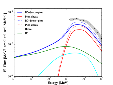
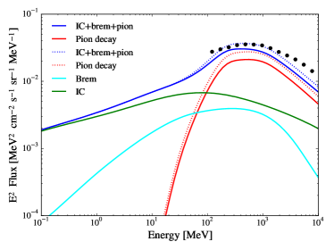
Figure 12: Predictions of the interstellar emission for the energy range of e-ASTROGAM and AMEGO gamma-ray instruments for PDDE model. Top: intermediate latitudes (10^∘$<|b|<$20^∘) for baseline PDDE model (solid lines) and for PDDE model with enhanced protons (dashed lines) that reproduces the gamma-ray emissivity. The different components are pion decay (red), bremsstrahlung (cyan), IC (green), and total interstellar (blue). Data are Fermi LAT spectra for intermediate regions from Ackermann et al. (2012) (black points). Data include statistical (grey area) and systematic errors (black bars). Bottom: predictions for the inner Galaxy (10^∘ radius around the Galaxy centre) for baseline PDDE model (solid lines) and for PDDE model with enhanced protons (dashed lines). The different components are as in the top figure. The e-ASTROGAM extended-source sensitivity is below the plotted intensity (see text for more details). Other components of the gamma-ray sky are not plotted.

5 Discussions and Conclusions

In this work CR propagation models consistent with recent CR measurements are tested against selected available data of the interstellar emission in radio and in gamma rays simultaneously. For the first time, this work shows that this is a feasible approach, which leads to fundamental model constraints, but it also introduces additional challenges. In more detail, we perform this study by comparing propagation models with spectral data of the local gamma-ray HI emissivity and synchrotron observations at intermediate latitudes. This approach allows obtaining the all-electron LIS, especially in the range (2 – 10⁵) MeV with no assumption on solar modulation. This enables us to test and constrain propagation models. Some models consistent with CR measurements only are disfavored, while other models can be put forward. Even though two of our models (PDDE and DRELowV) represent at best the data, we do not find a unique model that can reproduce all the observables at a time.

The main results from this study are:
(1) The injection spectral index of primary CR electrons need at least a break below a few GeV. Models with no breaks are excluded because they over-predict Voyager 1 CR all-electron measurements. Our DRC model (diffusion + convection + reacceleration) and our DRE model (diffusion + reacceleration) require two breaks in order to reproduce CR data, while our PDDE model (diffusion only) requires one break only.
(2) Models with a high all-electron LIS intensity in the $\sim$(10²–10⁴) MeV range, and hence models that produce a large amount of secondary electrons and positrons, are excluded by both synchrotron and gamma ray observations, even though in agreement with direct CR measurements. This affects reacceleration models with Alfven velocity with the typical value of $\sim$ 30 – 40 km/s for protons. The consequence is that models with reacceleration need significantly different propagation parameters for low-mass isotope data and for light elements (including secondary-to-primary ratios) in order to be supported by CR measurements, synchrotron and gamma-ray data. On the other hand, the all-electron LIS produced by usual plain diffusion models is supported by CR measurements, and also by synchrotron and gamma-ray data, adopting the same propagation parameters for low-mass isotopes and light elements. We provide our resulting favorite all-electron LIS based on local synchrotron, gamma-ray data, and direct CR measurements. Our finding that some recent propagation models consistent with CR measurements are not supported by multiwavelength observations suggests future propagation parameters studies to be checked against both radio and gamma-ray observations.
(3) The calculated spectrum of the local gamma-ray emissivity above $\sim$1 GeV due to pion decay produced by CRs as precisely measured by AMS-02 is lower than observed, even if accounting for solar modulation. The overall normalization of the proton spectrum derived to fit the emissivity data in the high-energy region free from modulation is $\sim$ 1.3 – 1.4. This indicates that the direct CR measurements do not represent the average spectrum in the local region within $\sim$1 kpc probed by the local gamma-ray emissivity. We provide the normalized proton spectrum that best-fit gamma-ray emissivity data.

As a general result we identify a preferred propagation model, PDDE, which is a plain diffusion model. This model with enhanced proton spectrum is finally in agreement with synchrotron and gamma-ray data. In Appendix we provide a table with the all-electron and proton spectra for PDDE model. An attempt to identify a model with reacceleration, DRELowV, provides results as good as the PDDE model.

We discuss further outcomes driven by this study.
(4) For most of the propagation models used in this work (DRE, DRC, DRELowV), by comparing the modeled electron LIS to AMS-02 measurements (Figure 2) it is possible to note that solar modulation on positrons has to be much larger than on electrons. This could imply that positrons have to be modulated differently than electrons in order to fit CR measurements at Earth. This might hint the evidence for a charge dependent modulation, and hence the need for a heliospheric propagation scenario more complex than usually assumed. However, this charge effect is not evident for models with no reacceleration as the PDDE model.
(5) In the Galactic centre region in gamma rays, models having low density of all-electrons in the $\sim$(10²–10⁴) MeV range (i.e. PDDE and DRELowV models) may be favored by Fermi LAT data at energies below 500 MeV, while in the same energy range DRE and DRC may be disfavored overproducing gamma rays. However, for PDDE and DRELowV models, enhancing the ISRF as supported by SPI and COMPTEL data produces many gamma rays in the 100 – 500 MeV energy band, which may be against observations. This is because an enhanced ISRF would enhance the IC emission at all energies. This may solve the degeneracy between CR all-electrons and ISRF, supporting the high-energy CR electron origin, and disfavoring the ISRF origin, of the enhanced IC emission found by Ajello et al. (2016) in the Galactic centre region above 1 GeV. However, the Galactic centre is a very complicated region, and it needs further dedicated works in order to finally probe CR density and spectra there. The Galaxy is optically thin, hence, when looking at the Galactic centre the interstellar emission acts both as foreground and as background because of the large integration length. The spatial computations of the gamma-ray emission in this work, as usually done, relay in the 2D azimuthally symmetric distributions of CR sources available in the public version of GALPROP. More sophisticated 3D CR source distributions could make some differences in the spatial distribution of the emission, and may be investigated in future studies. We have verified that for usual 2D CR source distributions, as used in Ackermann et al. (2012) and in all the works cited above, the spectrum of the calculated gamma-ray emission is not affected by the assumed CR source distribution. While the Galactic centre is an interesting sky region, it also is a very complicated area where to draw final conclusions upon. Moreover, the modeling in this region suffers from large uncertainties given by the gas density along the line of sight. Hence, while we qualitatively discuss the comparison of interstellar models with data, we do not draw any new final conclusion by looking at this region alone, which would need a dedicated and more sophisticated work. In addition, the influence on CRs of Galactic winds and of a possible anisotropy of the diffusion coefficient can be relevant. For instance, the possibility to launch CR-induced winds in the Galactic environment has been investigated in very recent works (e.g. Recchia et al., 2017). Physical conditions (e.g. Pfrommer et al., 2017; Girichidis et al., 2016) can be different from the models used in our work. As an example, recent Galaxy formation simulations (e.g. Pakmor et al., 2016) showed that with an anisotropic diffusion most CRs remain in the disk having important consequences for the gas dynamics in the disk, while with an isotropic diffusion CRs are allowed to quickly diffuse out of the disk. This could have unpredictable consequence to our modeling. However, implementing such effects is beyond the present effort.
(6) The X-ray to soft gamma-ray intensity of the diffuse emission in the inner Galaxy observed by SPI and COMPTEL is well reproduced by the IC emission of models having a large all-electron density in the $\sim$(10²–10⁴) MeV range (DRE and DRC models). However these models are in tension with the observed local gamma-ray emissivity and with the observed synchrotron emission. This could suggest that SPI and COMPTEL diffuse data in the inner Galaxy region are affected by source contamination of unresolved sources (due to the well-known limited sensitivity and angular resolution of the instruments), which would mimic the IC emission produced by the enhanced all-electron density in the $\sim$(10²–10⁴) MeV range of the DRE and DRC models. Such a possible contaminating source population in the SPI and COMPTEL energy band could be the soft gamma-ray pulsars that were found to have hard power-law spectra in the hard X-ray band and reach maximum luminosities typically in the MeV range (Kuiper & Hermsen, 2015). The presence of one or more sources of low-energy CR all-electrons in the inner Galaxy region only could also boost the resulting integrated IC component at X-ray energies, but this would also boost the bremsstrahlung component at few hundred MeV energies, which again would not be supported by Fermi LAT data in the Galactic center region (see previous point). However, while the inner Galaxy is an interesting sky region, it also is a very complicated area where to draw final conclusions upon. Dedicated analyses and more sensitive observations of the inner Galaxy in the MeV range would be needed in order to have a much clearer picture of this region.
(7) In an effort to make predictions for the newly proposed MeV missions, e-ASTROGAM and AMEGO, we have also explored our models at energies below 100 MeV. The sky above 100 MeV is dominated by the emission produced by CRs interacting with the gas and the ISRF via pion-decay, IC, and bremsstrahlung. Disentangling the different components at the LAT energies is challenging and is usually done in a model-dependent approach. Uncertainties in the interstellar medium is the major limitation to such a modeling and hence in our knowledge of CRs (e.g. Ackermann et al., 2012). The situation below 100 MeV is still unexplored. Predictions of present models to such low energies show IC and bremsstrahlung to be the major mechanisms of CR-induced emission, which are of leptonic origin. With their improved PSF and energy resolution e-ASTROGAM and/or AMEGO will finally be able to access those energies that have never been studied after the COMPTEL era.

The results in this work are important also for future dedicated studies of diffuse emissions in general. In fact, propagation models, as our PDDE and DRELowV models, could be used as baseline models to assess uncertainties of the gamma-ray interstellar emission in the entire sky, for example for studies regarding diffuse gamma-ray emissions (e.g. Ajello et al., 2016) and extended sources (e.g. Acero et al., 2016a).

Appendix

We report the LIS of all-electrons and protons for the favorite model PDDE in Table 5 and Table 6 respectively. The proton spectrum scaled to fit the local gamma-ray emissivity is reported in Table LABEL:TableApp3.

Table 5: All-electron spectrum for PDDE model that fits CR measurements, synchrotron emission and gamma ray emissivity, as plotted in Figure 2. The first column is the kinetic energy and the second column is the spectral intensity multiplied by E².

E	Intensity
(MeV)	(MeV2cm-2s-1sr-1Mev-1)
2.9243	0.948432171
3.4969	1.09652327
4.1817	1.263044372
5.0006	1.450084145
5.9799	1.6601582
7.151	1.89549382
8.5513	2.15923726
10.226	2.45476391
12.228	2.7857931
14.623	3.15681
17.487	3.5728002
20.911	4.0395083
25.006	4.563631
29.903	5.153056
35.759	5.81666
42.762	6.562885
51.136	7.389989
61.15	8.23707
73.125	8.67137
87.445	8.93157
104.57	9.20788
125.05	9.49295
149.54	9.77528
178.82	10.04511
213.84	10.30112
255.71	10.54979
305.79	10.79938
365.67	11.05006
437.28	11.29157
522.92	11.51173
625.32	11.69561
747.77	11.82816
894.21	11.89636
1069.3	11.88194
1278.7	11.76445
1529.1	11.51491
1828.6	11.10544
2186.7	10.51503
2614.9	9.74485
3127.0	8.81966
3739.3	7.78374
4471.6	6.67781
5347.3	5.48447
6394.5	4.39294
7646.7	3.51204
9144.1	2.80351
10935.0	2.235134
13076.0	1.780259
15637.0	1.416798
18699.0	1.126881
22361.0	0.895903
26740.0	0.711662
31976.0	0.565024
38238.0	0.448214
45727.0	0.36064
54681.0	0.2822996
65389.0	0.2236471
78195.0	0.1770424
93507.0	0.1400206
111820.0	0.1106436
133720.0	0.0873381
159900.0	0.0688765
191220.0	0.0542632
228660.0	0.04271027
273440.0	0.03358651
326990.0	0.02638933
391020.0	0.02071834
467600.0	0.0162543
559170.0	0.01274445
Concluded

Table 6: Proton spectrum for baseline PDDE model that fits CR measurements, but it does not fit the local emissivity, as plotted in Figure 1. The first column is the kinetic energy and the second column is the spectral intensity multiplied by E².

E	Intensity
(MeV)	(MeV2cm-2s-1sr-1Mev-1)
29.903	2.389
35.759	3.4093
42.762	4.8157
51.136	6.7323
61.15	9.3142
73.125	12.752
87.445	17.285
104.57	23.211
125.05	30.913
149.54	40.877
178.82	53.733
213.84	70.31
255.71	91.668
305.79	119.1
365.67	154.46
437.28	199.75
522.92	256.4
625.32	318.41
747.77	335.54
894.21	354.13
1069.3	373.29
1278.7	391.29
1529.1	407.45
1828.6	421.3
2186.7	432.31
2614.9	440.01
3127.0	443.85
3739.3	442.27
4471.6	396.72
5347.3	333.52
6394.5	299.64
7646.7	275.33
9144.1	251.15
10935.0	227.61
13076.0	205.08
15637.0	183.82
18699.0	164.02
22361.0	145.75
26740.0	129.05
31976.0	113.93
38238.0	100.31
45727.0	88.117
54681.0	77.257
65389.0	67.623
78195.0	59.106
93507.0	51.599
111820.0	44.996
133720.0	39.202
159900.0	34.128
191220.0	29.692
228660.0	25.818
273440.0	22.438
326990.0	19.493
391020.0	16.929
467600.0	14.697
559170.0	12.757
668670.0	11.07
799610.0	9.6046
956200.0	8.3318
Concluded

Table 7: Proton spectrum obtained from the emissivity, as plotted in Figure 6. The first column is the kinetic energy and the second column is the spectral intensity multiplied by E².

E	Intensity
(MeV)	(MeV2cm-2s-1sr-1Mev-1)
894.21	460.369
1069.3	485.277
1278.7	508.677
1529.1	529.685
1828.6	547.69
2186.7	562.003
2614.9	572.013
3127.0	577.005
3739.3	574.951
4471.6	515.736
5347.3	433.576
6394.5	389.532
7646.7	357.929
9144.1	326.495
10935.0	295.893

References

- Abazajian et al. (2014) Abazajian, K. N., Canac, N., Horiuchi, S., & Kaplinghat, M. 2014, Phys. Rev. D, 90, 023526
- Abdo et al. (2009) Abdo, A. A., Ackermann, M., Ajello, M., et al. 2009, Physical Review Letters, 103, 251101
- Abdo et al. (2010) Abdo, A. A., Ackermann, M., Ajello, M., et al. 2010, ApJ, 710, 133
- Abdollahi et al. (2017) Abdollahi, S., Ackermann, M., Ajello, M., et al. 2017, Phys. Rev. D, 95, 082007
- Accardo et al. (2014) Accardo, L., Aguilar, M., Aisa, D., et al. 2014, Physical Review Letters, 113, 121101
- Acero et al. (2016) Acero, F., Ackermann, M., Ajello, M., et al. 2016, ApJS, 223, 26
- Acero et al. (2016a) Acero, F., Ackermann, M., Ajello, M., et al. 2016, ApJS, 224, 8
- Ackermann et al. (2010) Ackermann, M., Ajello, M., Atwood, W. B., et al. 2010, Phys. Rev. D, 82, 092004
- Ackermann et al. (2011) Ackermann, M., Ajello, M., Baldini, L., et al. 2011, ApJ, 726, 81
- Ackermann et al. (2012) Ackermann, M., Ajello, M., Atwood, W. B., et al. 2012, ApJ, 750, 3
- Ackermann et al. (2014) Ackermann, M., Albert, A., Atwood, W. B., et al. 2014, ApJ, 793, 64
- Ackermann et al. (2015) Ackermann, M., Ajello, M., Albert, A., et al. 2015, ApJ, 799, 86
- Ackermann et al. (2017) Ackermann, M., Ajello, M., Albert, A., et al. 2017, ApJ, 840, 43
- Ackermann et al. (2012) Ackermann, M., Ajello, M., Allafort, A., et al. 2012, Physical Review Letters, 108, 011103
- Adriani et al. (2009) Adriani, O., Barbarino, G. C., Bazilevskaya, G. A., et al. 2009, Nature, 458, 607
- Adriani et al. (2011) Adriani, O., Barbarino, G. C., Bazilevskaya, G. A., et al. 2011, Science, 332, 69
- Adriani et al. (2013) Adriani, O., Barbarino, G. C., Bazilevskaya, G. A., et al. 2013, ApJ, 765, 91
- Adriani et al. (2014) Adriani, O., Barbarino, G. C., Bazilevskaya, G. A., et al. 2014, ApJ, 791, 93
- Adriani et al. (2015) Adriani, O., Barbarino, G. C., Bazilevskaya, G. A., et al. 2015, ApJ, 810, 142
- Aguilar et al. (2013) Aguilar, M., Alberti, G., Alpat, B., et al. 2013, Physical Review Letters, 110, 141102
- Aguilar et al. (2014) Aguilar, M., Aisa, D., Alvino, A., et al. 2014, Physical Review Letters, 113, 121102
- Aguilar et al. (2015a) Aguilar, M., Aisa, D., Alpat, B., et al. 2015, Physical Review Letters, 115, 211101
- Aguilar et al. (2015b) Aguilar, M., Aisa, D., Alpat, B., et al. 2015, Physical Review Letters, 114, 171103
- Aguilar et al. (2016) Aguilar, M., Ali Cavasonza, L., Ambrosi, G., et al. 2016, Physical Review Letters, 117, 231102
- Aloisio & Blasi (2013) Aloisio, R., & Blasi, P. 2013, J. Cosmology Astropart. Phys., 7, 001
- Alvarez et al. (1997) Alvarez, H., Aparici, J., May, J., & Olmos, F. 1997, A&AS, 124, 205
- Atwood et al. (2009) Atwood, W. B., Abdo, A. A., Ackermann, M., et al. 2009, ApJ, 697, 1071
- Ajello et al. (2016) Ajello, M., Albert, A., Atwood, W. B., et al. 2016, ApJ, 819, 44
- Bobik et al. (2016) Bobik, P., Boschini, M. J., Della Torre, S., et al. 2016, Journal of Geophysical Research (Space Physics), 121, 3920
- Boschini et al. (2017a) Boschini, M. J., Della Torre, S., Gervasi, M., et al. 2017, eprint (arXiv:1708.04690). Proceedings of IAU Symposium 335
- Bennett et al. (2013) Bennett, C. L., Larson, D., Weiland, J. L., et al. 2013, ApJS, 208, 20
- Bertone (2010) Bertone, G. 2010 Nature 468, 389
- Blasi (2013) Blasi, P. Astron Astrophys Rev 2013 21: 70.
- Boschini et al. (2017b) Boschini, M. J., Della Torre, S., Gervasi, M., et al. 2017, ApJ, 840, 115
- Bouchet et al. (2011) Bouchet, L., Strong, A. W., Porter, T. A., et al. 2011, ApJ, 739, 29
- Calore et al. (2015) Calore, F., Cholis, I., & Weniger, C. 2015, J. Cosmology Astropart. Phys., 3, 038
- Caprioli (2012) Caprioli, D. 2012, J. Cosmology Astropart. Phys., 7, 038
- Carlson et al. (2016) Carlson, E., Linden, T., & Profumo, S. 2016, Phys. Rev. D, 94, 063504
- Casandjian (2015) Casandjian, J.-M. 2015, ApJ, 806, 240
- Dickinson et al. (2015) Dickinson, C., et al. 2015, Advancing Astrophysics with the SKA (AASKA14), 102
- Cummings et al. (2016) Cummings, A. C., Stone, E. C., Heikkila, B. C., et al. 2016, ApJ, 831, 18
- De Angelis et al. (2017a) De Angelis, A., Tatischeff, V., Tavani, M., et al. 2017, Experimental Astronomy 44, 25
- De Angelis et al. (2017b) De Angelis, A., Tatischeff, V., Grenier, I. A., et al. 2017, arXiv:1711.01265
- Della Torre et al. (2015) Della Torre, S., Gervasi, M., Rancoita, P. G., Rozza, D., & Treves, A. 2015, Journal of High Energy Astrophysics, 8, 27
- Dermer et al. (2013) Dermer, C. D., Strong, A. W., Orlando, E., Tibaldo, L., & for the Fermi Collaboration 2013, arXiv:1307.0497. Proceedings of the 2013 ICRC conference.
- Di Mauro et al. (2016) Di Mauro, M., Donato, F., Fornengo, N., & Vittino, A. 2016, J. Cosmology Astropart. Phys., 5, 031
- Dobler et al. (2010) Dobler, G., Finkbeiner, D. P., Cholis, I., Slatyer, T., & Weiner, N. 2010, ApJ, 717, 825
- Donato et al. (2002) Donato, F., Maurin, D., & Taillet, R. 2002, A&A, 381, 539
- Donato & Serpico (2011) Donato, F., & Serpico, P. D. 2011, Phys. Rev. D, 83, 023014
- Engelmann et al. (1990) Engelmann, J. J., Ferrando, P., Soutoul, A., Goret, P., & Juliusson, E. 1990, A&A, 233, 96
- Evoli et al. (2017) Evoli, C., Gaggero, D., Vittino, A., et al. 2017, J. Cosmology Astropart. Phys., 2, 015
- Fornengo et al. (2014) Fornengo, N., Lineros, R. A., Regis, M., & Taoso, M. 2014, J. Cosmology Astropart. Phys., 4, 008
- Funk (2015) Funk, S. 2015, Annual Review of Nuclear and Particle Science, 65, 245
- Gaggero et al. (2014) Gaggero, D., Maccione, L., Grasso, D., Di Bernardo, G., & Evoli, C. 2014, Phys. Rev. D, 89, 083007
- Genolini et al. (2015) Genolini, Y., Putze, A., Salati, P., & Serpico, P. D. 2015, A&A, 580, A9
- George et al. (2009) George, J. S., Lave, K. A., Wiedenbeck, M. E., et al. 2009, ApJ, 698, 1666
- Girichidis et al. (2016) Girichidis, P., Naab, T., Walch, S., et al. 2016, ApJ, 816, L19
- Górski et al. (2005) Górski, K. M., Hivon, E., Banday, A. J., et al. 2005, ApJ, 622, 759
- Grenier et al. (2015) Grenier, I. A., Black, J. H., & Strong, A. W. 2015, ARA&A, 53, 199
- Guzmán et al. (2011) Guzmán, A. E., May, J., Alvarez, H., & Maeda, K. 2011, A&A, 525, A138
- Jaffe et al. (2011) Jaffe, T. R., Banday, A. J., Leahy, J. P., Leach, S., & Strong, A. W. 2011, MNRAS, 416, 1152
- Johannesson et al. (2015) Johannesson, G., Moskalenko, I. V., Orlando, E., Porter, T., & Strong, A. 2015, 34th International Cosmic Ray Conference (ICRC2015), 34, 517
- Jóhannesson et al. (2016) Jóhannesson, G., Ruiz de Austri, R., Vincent, A. C., et al. 2016, ApJ, 824, 16
- Haslam et al. (1981) Haslam, C. G. T., Klein, U., Salter, C. J., et al. 1981, A&A, 100, 209
- Haslam et al. (1982) Haslam, C. G. T., Salter, C. J., Stoffel, H., & Wilson, W. E. 1982, A&AS, 47, 1
- Irfan et al. (2015) Irfan, M. O., Dickinson, C., Davies, R. D., et al. 2015, MNRAS, 448, 3572
- Kamae et al. (2006) Kamae, T., Karlsson, N., Mizuno, T., Abe, T., & Koi, T. 2006, ApJ, 647, 692
- Kissmann et al. (2015) Kissmann, R., Werner, M., Reimer, O., & Strong, A. W. 2015, Astroparticle Physics, 70, 39
- Kuiper & Hermsen (2015) Kuiper, L., & Hermsen, W. 2015, MNRAS, 449, 3827
- Landecker & Wielebinski (1970) Landecker, T. L., & Wielebinski, R. 1970, Australian Journal of Physics Astrophysical Supplement, 16, 1
- Linden et al. (2016) Linden, T., Rodd, N. L., Safdi, B. R., & Slatyer, T. R. 2016, Phys. Rev. D, 94, 103013
- Lipari (2017) Lipari, P. 2017, Phys. Rev. D, 95, 063009
- Lorimer et al. (2006) Lorimer, D. R., Faulkner, A. J., Lyne, A. G., et al. 2006, MNRAS, 372, 777
- Maeda et al. (1999) Maeda, K., Alvarez, H., Aparici, J., May, J., & Reich, P. 1999, A&AS, 140, 145
- Pohl & Esposito (1998) Pohl, M., & Esposito, J. A. 1998, ApJ, 507, 327
- Maurin et al. (2010) Maurin, D., Putze, A., & Derome, L. 2010, A&A, 516, A67
- Mori (2009) Mori, M. 2009, Astroparticle Physics, 31, 341
- Mertsch & Sarkar (2014) Mertsch, P., & Sarkar, S. 2014, Phys. Rev. D, 90, 061301
- Mori (1997) Mori, M. 1997, ApJ, 478, 225
- Moskalenko & Strong (1998) Moskalenko, I. V., & Strong, A. W. 1998, ApJ, 493, 694
- Moskalenko et al. (1998) Moskalenko, I. V., Strong, A. W., & Reimer, O. 1998, A&A, 338, L75
- Moskalenko & Strong (2000) Moskalenko, I. V., & Strong, A. W. 2000, ApJ, 528, 357
- Moskalenko et al. (2002) Moskalenko, I. V., Strong, A. W., Ormes, J. F., & Potgieter, M. S. 2002, ApJ, 565, 280
- Moskalenko et al. (2015) Moskalenko, I. V., Jóhannesson, G., Orlando, E., et al. 2015, 34th International Cosmic Ray Conference (ICRC2015), 34, 492
- Orlando & Strong (2013) Orlando, E., & Strong, A. 2013, MNRAS, 436, 2127
- Pakmor et al. (2016) Pakmor, R., Pfrommer, C., Simpson, C. M., & Springel, V. 2016, ApJL, 824, L30
- Parker (1958) Parker, E. N. 1958, Physical Review, 110, 1445
- Pfrommer et al. (2017) Pfrommer, C., Pakmor, R., Schaal, K., Simpson, C. M., & Springel, V. 2017, MNRAS, 465, 4500
- Picozza et al. (2007) Picozza, P., Galper, A. M., Castellini, G., et al. 2007, Astroparticle Physics, 27, 296
- Planck Collaboration et al. (2016) Planck Collaboration, Ade, P. A. R., Aghanim, N., et al. 2016, A&A, 594, A25
- Planck Collaboration et al. (2016a) Planck Collaboration, Adam, R., Ade, P. A. R., et al. 2016, A&A, 594, A10
- Porter et al. (2008) Porter, T. A., Moskalenko, I. V., Strong, A. W., Orlando, E., & Bouchet, L. 2008, ApJ, 682, 400
- Ptuskin et al. (2006) Ptuskin, V. S., Moskalenko, I. V., Jones, F. C., Strong, A. W., & Zirakashvili, V. N. 2006, ApJ, 642, 902
- Putze et al. (2010) Putze, A., Derome, L., & Maurin, D. 2010, A&A, 516, A66
- Recchia et al. (2017) Recchia, S., Blasi, P., & Morlino, G. 2017, MNRAS, 470, 865
- Reich (1982) Reich, W. 1982, A&AS, 48, 219
- Reich et al. (2001) Reich, P., Testori, J. C., & Reich, W. 2001, A&A, 376, 861
- Remazeilles et al. (2015) Remazeilles, M., Dickinson, C., Banday, A. J., Bigot-Sazy, M.-A., & Ghosh, T. 2015, MNRAS, 451, 4311
- Roger et al. (1999) Roger, R. S., Costain, C. H., Landecker, T. L., & Swerdlyk, C. M. 1999, A&AS, 137, 7
- Schönfelder et al. (2000) Schönfelder, V., Bennett, K., Blom, J. J., et al. 2000, A&AS, 143, 145
- Schoenfelder et al. (1993) Schoenfelder, V., Aarts, H., Bennett, K., et al. 1993, ApJS, 86, 657
- Singal et al. (2011) Singal, J., Fixsen, D. J., Kogut, A., et al. 2011, ApJ, 730, 138
- Stone et al. (1977) Stone, E. C., Vogt, R. E., McDonald, F. B., et al. 1977, Space Sci. Rev., 21, 355
- Strong et al. (1999) Strong, A. W., Bloemen, H., Diehl, R., Hermsen, W., & Schönfelder, V. 1999, Astrophysical Letters and Communications, 39, 209
- Strong et al. (2004) Strong, A. W., Moskalenko, I. V., Reimer, O., Digel, S., & Diehl, R. 2004, A&A, 422, L47
- Strong et al. (2007) Strong, A. W., Moskalenko, I. V., & Ptuskin, V. S. 2007, Annual Review of Nuclear and Particle Science, 57, 285
- Strong et al. (2011) Strong, A. W., Orlando, E., & Jaffe, T. R. 2011, A&A, 534, A54
- Strong (2015) Strong A. W. for the Fermi LAT Collaboration, Contribution to the 34th International Cosmic Ray Conference, July 30 to August 6, The Hague, Netherlands (arXiv:1507.05006)
- Su et al. (2010) Su, M., Slatyer, T. R., & Finkbeiner, D. P. 2010, ApJ, 724, 1044
- Tibaldo et al. (2015) Tibaldo, L., Digel, S. W., Casandjian, J. M., et al. 2015, ApJ, 807, 161
- Tomassetti (2015) Tomassetti, N. 2015, Phys. Rev. D, 92, 063001
- Vedrenne et al. (2003) Vedrenne, G., Roques, J.-P., Schönfelder, V., et al. 2003, A&A, 411, L63
- Vidal et al. (2015) Vidal, M., Dickinson, C., Davies, R. D., & Leahy, J. P. 2015, MNRAS, 452, 656
- Vladimirov et al. (2011) Vladimirov, A. E., Digel, S. W., Jóhannesson, G., et al. 2011, Computer Physics Communications, 182, 1156
- Vladimirov et al. (2012) Vladimirov, A. E., Jóhannesson, G., Moskalenko, I. V., & Porter, T. A. 2012, ApJ, 752, 68
- Winkler et al. (2003) Winkler, C., Courvoisier, T. J.-L., Di Cocco, G., et al. 2003, A&A, 411, L1
- Wehus et al. (2014) Wehus, I. K., Fuskeland, U., Eriksen, H. K., et al. 2014, arXiv:1411.7616
- Wehus et al. (2017) Wehus, I. K., Fuskeland, U., Eriksen, H. K., et al. 2017, A&A, 597, A131