Exploring High-Dimensional Structure via Axis-Aligned Decomposition of Linear Projections

Abstract

Two-dimensional embeddings remain the dominant approach to visualize high dimensional data. The choice of embeddings ranges from highly non-linear ones, which can capture complex relationships but are difficult to interpret quantitatively, to axis-aligned projections, which are easy to interpret but are limited to bivariate relationships. Linear project can be considered as a compromise between complexity and interpretability, as they allow explicit axes labels, yet provide significantly more degrees of freedom compared to axis-aligned projections. Nevertheless, interpreting the axes directions, which are linear combinations often with many non-trivial components, remains difficult. To address this problem we introduce a structure aware decomposition of (multiple) linear projections into sparse sets of axis aligned projections, which jointly capture all information of the original linear ones. In particular, we use tools from Dempster-Shafer theory to formally define how relevant a given axis aligned project is to explain the neighborhood relations displayed in some linear projection. Furthermore, we introduce a new approach to discover a diverse set of high quality linear projections and show that in practice the information of $k$ linear projections is often jointly encoded in $\sim k$ axis aligned plots. We have integrated these ideas into an interactive visualization system that allows users to jointly browse both linear projections and their axis aligned representatives. Using a number of case studies we show how the resulting plots lead to more intuitive visualizations and new insight.

Computer GraphicsI.3.3Picture/Image GenerationLine and curve generation

1 Introduction

With the ever-increasing emphasis on data-centric analysis, studying high dimensional data has become an ubiquitous problem in science and engineering. Traditional confirmatory data analysis [Tuk80] (i.e., confirm/reject an hypothesis) requires users to form relevant hypotheses before any analysis can be started. However, deriving an intuitive understanding of the data in order to form such hypotheses is becoming increasingly difficult. One common approach is to use (interactive) visual exploration to inspire new hypotheses and a large body of research has been focused on how to make this process as intuitive and effective as possible.

While there exist a wide range of different approaches, two-dimensional embeddings remain the most commonly used technique to explore high dimensional data. The goal is to allow the user to reason about high-dimensional relationships and structures, i.e., correlations, clusters, etc., in a low dimensional, less abstract context. To aid the user in obtaining new insights, these embeddings need to be both accurate, i.e., reflect the high-dimensional structures, and intuitive, i.e., allow for an easy interpretation. Unfortunately, these two goals often conflict in practice. On one end of the spectrum non-linear embeddings, e.g., t-distributed stochastic neighborhood embedding (t-SNE) [MH08] and multi-dimensional scaling (MDS) [KW78], are good at capturing complex relationships. However, the resulting embeddings are difficult to interpret quantitatively as directions in the plot do not necessarily correspond to any coordinate, and distances can be severely distorted. Conversely, axis-aligned projections are straightforward to interpret, yet are very limited in the type of relationships they can highlight.

Linear projections are often considered a good compromise between both objectives as they can arbitrarily increase the degrees of freedom to find high dimensional relationships, while directly relating directions in the plot to the original coordinates. Though the distances in a linear projection are easy to interpret, the axes often correspond to linear combinations of dozens of dimensions, many of which are expressed equally strong. Consequently, this requires a user to simultaneously reason about many different attributes which is often overwhelming. One common approach aiming to address this challenge is to enforce sparsity in both axes of a plot by preferring linear projections with fewer constituent coordinates [CG05]. However, this reduces the expressive power of the resulting linear projections and unless taken to the extreme often still results in too many relevant coordinate directions to be intuitive.

An attractive alternative is to consider a given linear projection in light of several similar axis-aligned projections. However, the straightforward solution of constructing a scatterplot matrix from all (significant) constituent coordinate directions typically results in too many combinations to be practical. Furthermore, there is little control over how accurate the resulting plots represent the true structure and many projections might be misleading rather than helpful. Instead, we introduce a new approach to approximate a linear projection with a small number of axis-aligned projections via generalization of sparse representations to the Riemannian space of linear projections [TG07], coupled with a greedy dimension selection technique. Furthermore, independent of how well the user can interpret a single linear projection, as corroborated by several recent related works [NM13, LWT^∗15, WM17, LT16, LBJ^∗16], an effective exploration of most high dimensional data requires a diverse set of views. To this end, we extend the decomposition approach to the case of multiple linear projections with additional constraint to reduce duplicated axis-aligned presentation. In particular, we define a measure of evidence using Dempster-Schafer theory to convey how much of the information from multiple linear projection is explained by a certain axis-aligned one. In addition, we introduce a new optimization approach to construct multiple linear projections that are both accurate and diverse. Unlike existing approaches, we do not focus exclusively on diversity [LT16], which may lead to projections with poor embedding quality, nor do we require a dense sampling of all possible projections [LBJ^∗16], or expensive subspace clustering computation [NM13, LWT^∗15, WM17]. Instead, we introduce an iterative optimization to explore the Grassmannian (i.e., the space of all linear projections) with any convex embedding objective, e.g., PCA (principal component analysis), LPP (locality preserving projection). We achieve the co-optimization of both diversity and quality, while still maintaining the convexity for each iteration to solve the problem efficiently.

Finally, we integrate our approaches into an interactive visual analytics interface that allows users to easily and intuitively interpret high dimensional data through a multi-faceted lens of linear and axis-aligned projections. Our contributions in detail are:

• A mathematical framework for representing a linear subspace as a sparse set of axis-aligned subspaces in a structure-aware manner;

• An optimization algorithm for identifying a diverse set of linear projections by simultaneously maximizing the accuracy and diversity of the projections;

• A visualization tool that exploits benefits of both the linear and axis-aligned projections by summarizing the relationships between the selected diverse set of linear projections and their corresponding axis-aligned projections.

2 Related Work

Generating low-dimensional embeddings of high-dimensional data is an extensively studied area in many related fields such as data mining, machine learning, and visualization. In the visualization community, instead of focusing solely on the general objective of dimensionality reduction, considerable efforts have been devoted to user-driven exploration and interpretation of high-dimensional data. In this section, we will discuss related approaches that rely on both axis-aligned and linear projections for exploratory analysis.

2.1 Axis-Aligned Projection

Scatterplot matrix (SPLOMs) is one of the most popular methods for visualizing high-dimensional data, where each plot is an axis-align projection. However, due to the quadratic increase in the number of plots as dimension grows, several methods (e.g., Scagnostics [WAG05] and rank-by-feature framework [SS04]) have been proposed to help identify "interesting" plots that are worthy of the user’s attention. Scagnostics [WAG05], supplies the user with multiple types of measures, e.g., clumpy, skinny, each capturing a specific pattern in the scatterplot. Combined, the different measures help user select a diverse set of axis-aligned projections. For an extensive review of the various quality measures, please refer to the survey articles [BTK11, LMW^∗17].

Compared to the well-known approaches that rely on ranking quality measures, the proposed approach is fundamentally different. Instead of filtering directly on all axis-aligned projections, we search for structures in the space of linear projections and then use axis-aligned projections to help explain the structure observed in them. In other words, linear projections are used as a guide for discovering diverse views of the data and as a bridge to connect the high-dimensional space with axis-aligned projections. For data with relative high-dimensions, the linear projection stage also helps avoid the quadratic complexity of the scatterplot matrix.

2.2 Linear Projection

Many widely adopted dimension reduction methods, such as principal component analysis [AW10] and Fisher’s discriminant analysis [MRW^∗99], are linear in nature. These methods are often easy to compute and capture structures that are of great interest for analysis (e.g., linear correlation, clusters in subspaces). However, a single linear projection only provides a limited view of the data, and hence might not reveal other important structures. As a result, several visualization approaches have resorted to creating multiple 2D projections or a series of projections (often referred to as a tour) to provide a more comprehensive view of the data. The classical Grand Tour method [Asi85] visualizes data through a series of 2D projections that explore the space of all linear projections in a space-filling manner. However, due to the size such a space, a complete tour may not be possible, even in moderate dimensions.

Instead of aiming for a complete tour, an alternative approach is to devise a measure to identify “interesting” projections. In the projection pursuit, we seek for 2D projections by optimizing a quality measure function [FT74]. One example is the Holes measure [CBC93], which finds projections where there is a gap between two clusters of points. For a given measure, the global extrema provides the user with only one view of the data. In order to address this limitation, the Grassmannian Atlas framework [LBJ^∗16], adopts tools from topological data analysis, in lieu of the global optimization, and identifies multiple local extrema of the quality measure, thus identifying a complementary set of linear projections. Recently, subspace clustering/selection based methods [LWT^∗15, TMF^∗12, NM13, YRWG13, WM17], have enabled structure-driven exploration, particularly while identifying important linear projections. Broadly, these methods decompose the high-dimensional data into lower-dimension subsets and project them separately to focus on local features. Besides using structure/pattern based quality measures to determine “interesting” projections, one can also explicitly consider diversity as an objective in the view optimization process. For example, Lehmann et al. [LT16] proposed to construct a set of 2D projections that are most dissimilar to each other after accounting for rotation and translation of the views. However, by not considering the quality of the resulting embeddings, this approach can produce views that do not strongly agree with the structure in high dimensions. Compared to the existing methods, the proposed algorithm considers both the quality, i.e., how well the current projection preserve neighborhood structure, and diversity, i.e., maximal separation from the previously selected ones, of the projections.

Reasoning about the meaning of the axes that are expressed as linear combinations of many different properties can be very challenging. Existing methods [Mor92, CG05] aim to reduce the number of non-zero components in the linear combination. In particular, the interpretable dimensionality reduction technique [CG05] employs an explicit sparse constraint to the linear projection bases, which yield simpler coordinates for the analysis. However, these techniques do not resolve the fundamental burden of interpreting axes as linear combinations, which can be particularly challenging in high dimensions. In contrast, the proposed method provides a set of axis-aligned projections that are inherently easier to interpret, while being maximally descriptive of the linear projections that guided their selection.

3 Axis-Aligned Decomposition of a Linear Projection

As discussed above, the overarching goal is to find a set of axis-aligned projections that jointly represent a linear projection well. A naive approach might use all pair-wise combinations of all dimensions that are active in a given linear projection. However, in practice, this will likely result in an overwhelming number of scatterplots. A more sophisticated variant of this idea is to use sparse coding on the Grassmannian manifold (the space of all linear subspaces) [HSSL13], which can be used to find a small set of axis-aligned projections. More specifically, let $\mathbf{V}$ be a basis of the linear subspace one is interested in and $\mathcal{Q}$ be the index set of all pair-wise combinations of dimensions, $|\mathcal{Q}|={d\choose 2}$, then to find the $L$ best axis-aligned subspaces, one can used the formulation of Harandi et al. [HSSL13]:

$$\boldsymbol{{\beta}}=\operatorname*{arg\,min}_{\{\beta_{i}\}}\|\mathbf{V}\mathbf{V}^{T}-\sum_{i=1}^{|\mathcal{Q}|}\beta_{i}\mathbf{Z}_{i}\mathbf{Z}_{i}^{T}\|_{F}^{2},$$

$$\text{subject to }\|\boldsymbol{\beta}\|_{0}\leq L.$$ (1)

Here $\mathbf{V}\mathbf{V}^{T}$ is the extrinsic representation for a point (a linear subspace) $\mathbf{V}$ on the Grassmannian and $\mathbf{Z}_{i}$ are axis-aligned subspaces. Note that this optimization is data independent, i.e., the error considers only the distance on the Grassmannian. This is not ideal for two reasons: First, the chosen $\mathbf{Z}_{i}^{\text{'s}}$ may result in poor projections either because they create significant distortions or their structure is not relevant to $\mathbf{V}$; and second, some of the $\mathbf{Z}_{i}^{\text{'s}}$ may result in very similar and thus redundant projections. The latter is common in data sets with highly correlated dimensions. Consider the extreme case of duplicated pairs of dimensions, which result in identical projections yet are maximally far apart on the Grassmannian. Instead, we propose to explicitly look for axis-aligned projections that encode the same structure as the given linear one. More specifically, we follow the approach shown in Figure 1: Given a linear subspace, we iteratively find a best matching axis-aligned one, remove its contribution from the linear projection on the Grassmannian to estimate the residual subspace and continue until no additional axis-aligned subspace can provide better structure preservation than the ones picked so far.

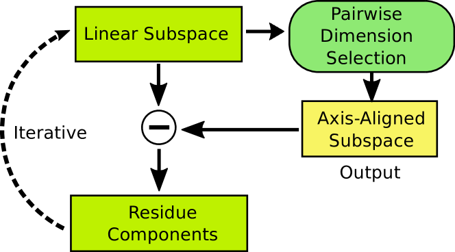
Figure 1: Illustration of the linear projection decomposition algorithm. Given a linear subspace, we iteratively find a best matching axis-aligned one, remove its contribution from the linear projection and continue until no additional axis-aligned subspace can provide better structure preservation than the ones picked so far.

3.1 Algorithm

We are interested in preserving the structure of a linear projection which we define as the set of all pairwise distances. Given a set of $n$ points $\mathbf{X}$ in $\mathbb{R}^{d}$ and the basis of a linear subspace $\mathbf{V}$, the projected coordinates $\mathbf{Y}$ are given as $\mathbf{Y}=\mathbf{V}^{T}\mathbf{X}$. The structure we want to preserve are pairwise distances $||\mathbf{y}_{i}-\mathbf{y}_{j}||^{2}$ for all $j,i\in{1,...,n}$, using a pair of dimensions from $\mathbf{X}$. In practice, we know that preserving all distances accurately is infeasible and thus we typically restrict the distances to a set of nearest neighbors, i.e., $j\in\mathcal{N}_{k}(i)$, where $\mathcal{N}_{k}(i)$ defines the $k$-nearest neighbors of $\mathbf{y}_{i}$ computed using the subspace defined by $\mathbf{V}$.

In order to find a pair of dimensions that best preserves the neighborhood distances we modify the image masking technique of [DD14]. Note that, for a uniformly distributed set of random masks of dimension $2$, i.e., can use only two of the $d$ dimensions in $\mathbf{X}$, one can expect a compaction factor of $\sqrt{{2}/{d}}$ in the true distances from $\mathbf{X}$. However, in our case, it is sufficient for the selected dimensions to agree with the structure of $\mathbf{Y}$. Hence, we start by defining the matrix $\mathbf{C}$ by stacking the set of difference vectors squared elementwise, $[(\mathbf{x}_{i}^{1}-\mathbf{x}_{j}^{1})^{2},...,(\mathbf{x}_{i}^{d}-\mathbf{x}_{j}^{d})^{2}]$, referred to as unnormalized secants, for all neighboring $i,j$ pairs. Similarly, we construct the unnormalized secants relative to the projection $\mathbf{V}$ and compute vector $\mathbf{b}$ with $\|\mathbf{y}_{i}-\mathbf{y}_{j}\|^{2}$. The optimal axis-aligned projection can then be found by optimizing:

$$\boldsymbol{{\alpha}}=\operatorname*{arg\,min}_{\boldsymbol{\alpha}}\|\mathbf{C}\boldsymbol{\alpha}-\mathbf{b}\|_{2}^{2}$$

$$\text{subject to}\qquad\mathbf{1}^{T}\boldsymbol{\alpha}=2,\boldsymbol{\alpha}\in\{0,1\}^{d}.$$ (2)

The non-zero entries in $\boldsymbol{{\alpha}}$ then indicate the two dimensions of the axis-aligned projection that best preserves the nearest-neighbor distances. Rather than solving this optimization directly as a binary integer program, we use a greedy procedure that selects one dimension of $\mathbf{X}$ at a time. The mask vector $\boldsymbol{{\alpha}}$ has a one-to-one correspondence with the index set $\mathcal{Q}$, and let us denote the corresponding index by $i_{{\alpha}}$. The axis-aligned subspace obtained is denoted by $\mathbf{Z}_{i_{\alpha}}\in\mathbb{R}^{d\times 2}$. We can now describe the full algorithm as shown below:

Algorithm 3.1

Optimize for $\Omega$ given $\mathbf{V}$ and $L$ (maximum number of axis-aligned subspaces)

1. Initialize axis -aligned projections $\Omega=\varnothing$, subspace $\mathbf{U}=\mathbf{V}$

2. While $|\Omega|\leq L$:

   1. Compute optimal $\mathbf{Z}_{i_{{\alpha}}}$ to approximate $\mathbf{U}$ using (2)

   2. Measure structural distortion $\|\mathbf{e}^{i}=\mathbf{C}\boldsymbol{\alpha}-\mathbf{b}^{i}\|_{2}$ for $\mathbf{U}$ and $\mathbf{Z}_{i_{{\alpha}}}$

   3. If $\mathbf{e}^{i}<\delta\min(\mathbf{e}^{j}),j\in\Omega$ and $\delta<1.0$, continue, else break

   4. Update set of axis-aligned projections: $\Omega\leftarrow\Omega\cup i_{\alpha}$

   5. Solve the least squares optimization in (3) and compute the residual on the Grassmannian: $\mathbf{R}=\mathbf{V}\mathbf{V}^{T}-\sum_{i\in\Omega}\beta_{i}\mathbf{Z}_{i}\mathbf{Z}_{i}^{T}$

   6. Reproject: Update $\mathbf{U}$ with two principal eigen vectors of $\mathbf{R}$

While the structural distortion metric is used to qualitatively evaluate the usefulness of the selected axis-aligned subspace in explaining the linear subspace, we estimate the residual subspace that could potentially contain information about the data, that is not described by the chosen axis-aligned subspace. This is carried out by first solving the following least squares optimization on the Grassmannian:

$$\boldsymbol{{\beta}}_{\Omega}=\operatorname*{arg\,min}_{\boldsymbol{\beta}}\|\mathbf{V}\mathbf{V}^{T}-\sum_{i\in\Omega}\beta_{i}\mathbf{Z}_{i}\mathbf{Z}_{i}^{T}\|_{F}^{2}+\lambda\|\boldsymbol{\beta}\|_{2},$$ (3)

and estimating the residual subspace as shown in steps 2e and 2f (Algorithm 3.1) respectively. However, the residual subspace need not always promote the selection of another relevant axis-aligned subspace, particularly when the dimensions are inherently correlated. In such cases, redundant axis-aligned subspaces with similar structure could be chosen. To avoid that behavior, in step 2c, we compare the structural distortion for the chosen axis-aligned subspace to those picked so far and terminate if there is no improvement in the distortion. Note that for some linear projections $\mathbf{V}$, there exists no good axis-aligned projections and the residual $\mathbf{R}$ remains high or even increases as more $\mathbf{Z}_{i}$s are added. Note that this does not mean there is no axis-aligned subspace close to $\mathbf{V}$, but rather they do not preserve the structure of $\mathbf{V}$. To combat this challenge, we set an upper bound on the number of axis-aligned subspaces that can be chosen. This novel combination of axis-subspace selection and residual computation enables a robust and high-quality decomposition.

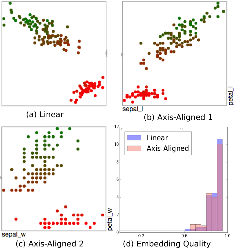
Figure 2: An example of the axis-aligned decomposition of a linear projection of iris dataset.

3.2 Example

We use a simple example dataset to intuitively illustrate the decomposition process. As shown in Figure 2, we decompose the LPP linear projection of the iris dataset (4D: sepal_w, sepal_l, petal_w, petal_l) into two structurally unique axis-aligned projections. As we can see, in Figure 2(b)(c), each of the axis-aligned projection uses two of unique dimensions in the 4D dataset.

The compactness (i.e., avoid duplication) of the axis-aligned representation is one important goal of the proposed algorithm. There are likely many axis-aligned projections that contain similar patterns in the iris data, however, the proposed technique ensures that each axis-aligned projection captures a unique structure. For the iris data example, in Figure 2, the axis-aligned projection (b) is extracted first. Structurally, it is very close to the linear one. After the contribution of the axis-aligned projection (b) is removed from the linear projection (a) using Grassmann analysis, the second axis-aligned projection (c) reveals a different pattern. In addition to being compact, the decomposition preserves the neighborhood structure from the linear projection with high fidelity. In order to demonstrate this, we compute the per-point precision-recall quality measure (see details in Section 5, the higher the value the better) of the linear projection with respect to the high dimensional data. Further, we evaluate the aggregated per-point measures from the corresponding axis-aligned projections. For the aggregation, we use the maximum of the quality measure for each point across the different axis-aligned projection. As showed in Figure 2(d), the histograms of the quality measure from both the cases highly overlap, indicating that for every point at least one of the axis-aligned projections captures the neighborhood relationship observed in the linear projection.

4 Decomposition of Multiple Linear Projections

In the previous section, we described our algorithm for identifying a concise set of axis-aligned projections that maximally describe the neighborhood structure observed in a given linear projection. However, as corroborated by several recent efforts [LT16, LWT^∗15, WM17], finding a diverse set of representative projections is crucial for obtaining a comprehensive understanding of high-dimensional data. Therefore, it is imperative to consider the scenario of obtaining a group of axis-aligned projections that jointly describe multiple linear projections of the data.

However, decomposition of multiple linear projections presents additional challenges. First, finding a desirable set of representative linear projections is very hard. Even though many existing methods try to identify multiple interesting projections of the data, none of them explicitly optimize for both the diversity (i.e., cover various aspects of the data) and the trustworthiness of the projection (i.e., make sure the projection is not misleading). Ignoring either of the objectives may lead to undesirable results. Second, the decomposition of multiple linear projections entails the risk of redundancy, i.e., multiple axis-aligned projections may capture similar structure, and the challenge of aggregation, i.e., measuring the importance of an axis-aligned projection that is part of multiple linear projection decompositions.

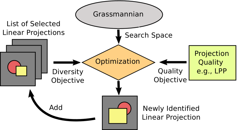
Figure 3: Illustration of the linear projection search algorithm.

In this section, we present our approach for finding multiple linear projections (see Figure 3) by jointly optimizing for embedding quality and diversity, using tools from Grassmann analysis. We generalize the algorithm in Section 3.2 by sequentially computing the decomposition for each of the linear projections. In this process, we avoid redundancy by promoting reuse of axis-aligned subspaces that were already chosen for another linear projection decomposition, thus producing a highly compact set of scatterplots for the user. Finally, we use tools from Dempster-Schafer theory to define an evidence measure, which aggregates the contributions of each axis-aligned projection to the multiple linear projections.

4.1 Finding Representative Linear Projections

Given the data matrix $\mathbf{X}\in\mathbb{R}^{d\times n}$, our criterion for obtaining representative linear projections is that the inherent structure of the data points is preserved. This ranges from recovering the directions of maximal variance (PCA) to neighborhood structure (Locality Preserving Projections [Niy04]) or class separation (Local Discriminant Embedding [CCL05]). Despite the varied nature of these techniques, all linear dimensionality reduction methods can be viewed through the lens of graph embedding.

In this approach, we represent each vertex of a graph as a low-dimensional vector that preserves relationships between the vertex pairs, where the relationship is measured by a similarity metric that characterizes certain statistical or geometric properties of the data set. Let $G=\{\mathbf{X},\mathbf{W}\}$ denote a undirected graph, where the matrix $\mathbf{W}\in\mathbb{R}^{n\times n}$ is the similarity matrix between all pairs of samples in $\mathbf{X}$. The Laplacian of the graph $G$ can be defined as $\mathbf{L}=\mathbf{D}-\mathbf{W}$, where $D_{ii}=\sum_{j\neq i}W_{ij}$. Denoting the linear projection by $\mathbf{V}$ and the corresponding embedding as $\mathbf{Y}=\mathbf{V}^{T}\mathbf{X}$, the problem of graph embedding can be written as:

$$\min_{tr(\mathbf{V}^{T}\mathbf{X}\mathbf{B}\mathbf{X}^{T}\mathbf{V})=\epsilon}tr(\mathbf{V}^{T}\mathbf{X}\mathbf{L}\mathbf{X}^{T}\mathbf{V}),$$ (4)

where $tr(.)$ denotes the trace operator, the matrix $\mathbf{B}$ corresponds to the Laplacian of an optional penalty graph, typically used to regularize the learning, and $\epsilon$ is a penalty constraint. The solution to (4) can be obtained using generalized eigenvalue decomposition. Table 1 lists the appropriate construction of the similarity graph and penalty graph Laplacians $\mathbf{L}$ and $\mathbf{B}$ for PCA, LPP and LDE.

Table 1: Formulating linear dimensionality reduction techniques using the unified graph embedding framework in [YXZ^∗07]

Method	Similarity Graph	Penalty Graph
PCA	$W_{ij}=1/n,i\neq j$	$\mathbf{B}=\mathbf{I}$
LPP	$W_{ij}=\exp(-\gamma\|\mathbf{x}_{i}-\mathbf{x}_{j}\|^{2})$, if $i\in\mathcal{N}(j)$ or $j\in\mathcal{N}(i)$	$\mathbf{B}=\mathbf{D}$
LDE	$W_{ij}=1,\text{ if }c_{i}=c_{j}$	$\mathbf{B}=\mathbf{D}^{\prime}-\mathbf{W}^{\prime}$, ${W}^{\prime}_{ij}=1,\text{ if }c_{i}\neq c_{j}$

However, since the intrinsic dimensionality of data is often greater than $2$, any 2D projection will invariably result in information loss. Hence, it is necessary to consider multiple 2D projections to obtain a more comprehensive view of the data. Similar to the approach in [LT16], we incorporate diversity as a quality measure to infer multiple projections. However, instead of comparing the structure of the two 2D projections, we propose to directly compare their corresponding subspaces on the Grassmannian manifold [YL14], while ensuring the embedding quality is not entirely compromised. We use the squared chordal distance to compare two subspaces $\mathbf{V}_{i}$ and $\mathbf{V}_{j}$ on the Grassmannian:

$$\rho^{2}(\mathbf{V}_{j},\mathbf{V}_{i}) =2-\|\mathbf{V}_{i}^{T}\mathbf{V}_{j}\|_{F}^{2}=2-\text{Tr}\left(\mathbf{V}_{j}^{T}\mathbf{V}_{i}\mathbf{V}_{i}^{T}\mathbf{V}_{j}\right).$$

Our algorithm begins by inferring a linear projection for $\mathbf{X}$ by solving (4) for the desired embedding objective, e.g. LPP. Subsequently, we find the second projection that not only a provides good quality embedding but is also far from the first subspace. Assuming that we need to compute the $(j+1)^{\text{th}}$ subspace, its diversity is measured as the sum of distances between that subspace and all the previous $i=\{1,\ldots,j\}$ subspaces, i.e.,

$$\sum_{i=1}^{j}\rho^{2}(\mathbf{V}_{j+1},\mathbf{V}_{i})=j2-\text{Tr}\left(\mathbf{V}_{j+1}^{T}\sum_{i=1}^{j}\left(\mathbf{V}_{i}\mathbf{V}_{i}^{T}\right)\mathbf{V}_{j+1}\right).$$

Hence, the optimization problem for computing the $j+1^{\text{th}}$ subspace is

$$\mathbf{V}_{j+1}=\operatorname*{arg\,min}_{\mathbf{V}^{T}\mathbf{X}\mathbf{B}\mathbf{X}^{T}\mathbf{V}=\epsilon}\text{Tr}\left(\mathbf{V}^{T}\left(\mathbf{X}\mathbf{L}\mathbf{X}^{T}+\alpha\sum_{i=1}^{j}\left(\mathbf{V}_{i}\mathbf{V}_{i}^{T}\right)\right)\mathbf{V}\right),$$ (5)

where $\alpha$ is the trade-off parameter between embedding quality and the dissimilarity between subspaces. Since the comparison on the Grassmannian is independent of the data, in some cases, two different subspaces that are well separated can still produce 2D projections with similar structure. In order to avoid choosing redundant subspaces, we also verify if the actual projection can be obtained through a simple affine transformation of one of the previously found projections.

4.2 Decomposition

Using the algorithm in Section 3.2, we obtain the decomposition of each of the linear projections into a set of relevant axis-aligned subspaces. Since each of the linear projections is processed independently, there is a risk of redundancy, i.e. multiple axis-aligned projections with a similar structure can be picked. We avoid this by maintaining a global set $\Omega^{G}$ that contains all axis-aligned subspaces previously chosen for any of the linear projections. For the next linear projection, we choose a new axis-aligned projection over any of the projections in $\Omega^{G}$, only when its structural preservation property is superior.

4.3 Inferring Evidence Measures

When considering the decomposition of multiple linear projections, the same axis-aligned subspace may contribute to more than one linear subspace. Therefore, to evaluate how much the axis-aligned subspace contributes to understanding the data on a whole, we propose to estimate evidence scores based on structural distortions.

Dempster-Shafer theory (DST) is a general framework for reasoning with uncertainty [S^∗76], which we will utilize to understand the degree of belief of each axis-aligned subspaces in describing the data. Let $\Theta$ be the universal set of all hypotheses, i.e., the set of all axis-aligned subspaces in our case, and $2^{\Theta}$ be its power set. A probability mass can be assigned to every hypothesis $A\in 2^{\Theta}$ such that, $\mu(\varnothing)=0,\sum_{A\in 2^{\Theta}}\mu(A)=1,$ where $\varnothing$ denotes the empty set. This measure provides the confidence that hypothesis $A$ is true. Using DST, we can compute the uncertainty of the axis-aligned subspaces in representing a linear subspace using the belief function, $\sum_{B\subseteq A}\mu(B)$, which is the confidence on that hypothesis being supported by strong evidence. Using principles from DST, we can easily combine the evidence from multiple sources. In our case, this corresponds to combining beliefs of an axis-aligned subspace in describing multiple linear subspaces.

Given the set of axis-aligned subspaces $\Omega$ for a linear subspace $\mathbf{V}$, the mass corresponding to the axis-aligned subspace $\mathbf{Z}_{i}$, where $i\in\Omega$ is given as $\mu(\mathbf{Z}_{i})$. This is estimated by computing the structural distortion $\mathbf{e}^{i}=\|\mathbf{C}\boldsymbol{\alpha}-\mathbf{b}^{i}\|_{2}$ and defining the mass $\eta$ to be the inverse of $\mathbf{e}^{i}$ defined as:

$$\eta=\eta_{0}\left(1-\frac{\mathbf{e}^{i}}{max(\{\mathbf{e}^{j}\}_{j\in\Omega})}\right)$$ (6)

Here $\eta_{0}$ is a parameter in the interval $[0,1]$ (chosen closer to $1$) that upper bounds the mass of any single hypothesis.

We apply Dempster’s combination rule to combine beliefs of $\mathbf{Z}_{i}$ from all linear projections. Assuming that there are $P$ linear subspaces denoted by the orthonormal bases $\{\mathbf{V}_{i}\}_{i=1}^{P}$, the total mass can be accumulated as

$$\mu(\mathbf{Z}_{i})=1-\prod_{p=1}^{P}\left(1-\eta_{0}\left(1-\frac{\mathbf{e}^{i}_{p}}{max(\{\mathbf{e}^{j}_{p}\}_{j\in\Omega,0\leq p<P})}\right)\right).$$ (7)

Here $\mathbf{e}^{i}_{p}$ denotes the structural distortion obtained for the $p^{\text{th}}$ linear projection using the $i^{\text{th}}$ axis-aligned subspace. Finally, the normalized evidence measure of the axis-aligned subspace $\mathbf{Z}_{i}$ is given by

$$evid[i]=\frac{\mu(\mathbf{Z}_{i})}{\max\left(\{\mu(\mathbf{Z}_{j})\}_{j=1}^{|\mathcal{Q}|}\right)},\forall i=1,\cdots,|\mathcal{Q}|.$$ (8)

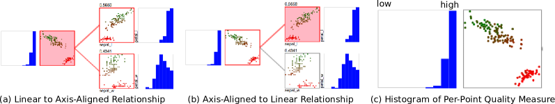
Figure 4: Projection Relationship View. As showed in (a)(b), the decomposition relationship is illustrated by a bipartite graph, the edges of the graph connect linear projections and their constituent axis-aligned projections from the proposed decomposition. The currently selected projection is highlighted with a red background. As illustrated in (c), for each projection, the histogram of per-point precision-recall quality measure is shown for illustrating how well a given projection preserves the neighborhood structure of the full dimensional data.

5 Projections Relationship Visualization

The previous sections discussed the computation pipeline that identifies diverse, representative linear projections and subsequently decomposes them into a compact set of axis-aligned projections. Though we can execute this pipeline directly as an offline analytic tool, visualizing the relationships between the linear and axis-aligned projections can not only present the computation results in a more accessible format but also help users develop additional insights. In this section, we discuss the design choice and the functionality for projection relationships visualization.

Design Goal. To design an effective visual encoding, it is important to first identify the exact information we want to communicate. For projection relationships, the key information we want to convey is the correspondence between a linear projection and its axis-aligned decomposition. One interesting property is the bi-directional nature of the relationships, i.e., a linear projection can be decomposed into multiple axis-aligned projections, while the same axis-aligned projection can also contribute to multiple linear projections.

Besides visualizing the connectivity among projections, we also want to help users develop a qualitative understanding of the structures captured in a linear projection via the decomposition into axis-aligned ones. Therefore, it is critical to broadly understand the point-wise correlation, i.e., which part of the linear embedding corresponds to the axis-aligned one. In particular, a meaningful animated transition from linear projection to the axis-aligned projection can help highlight such a relationship.

To achieve these two design goals, we devised two visualization components: the projection relationship view and the projection transition view. The functionality and the rationale for the design choices are discussed in the following sections.

Projection Relationship View. The projection relationship view provides an overview of the linear and axis-aligned projections and encodes their decomposition relationships. As discussed in Section 4, the proposed computation method first obtains the representative linear projections and then decomposes them into axis-aligned ones. To express the two stages in the computation and visually separate linear and axis-aligned projections, we encode the projections and their connections as a bipartite graph.

As illustrated in Figure Exploring High-Dimensional Structure via Axis-Aligned Decomposition of Linear Projections(a), the projections are encoded as nodes in the graph, where linear projections correspond to nodes on the left column, and the axis-aligned projections are nodes on the right column. Their decomposition relationship is expressed as edges in the bipartite graph. A natural advantage of such an encoding is that the bi-directional nature of the connectivity can be intuitively expressed. As illustrated in Figure 4(a)(b), we show the decomposition relationship from a linear (source) to axis-aligned projections (targets), as well as the aggregation relationship from an axis-aligned projection (source) to the linear ones (targets) it describes. The source (also the actively selected one) node are highlighted in light red and the edges from source to targets are displayed as red lines. In addition, the thickness of the line indicates the evidence contribution (discussed in Section 4.3) of the axis-aligned projections for explaining the structure of the associated linear projection. Finally, we allow the user to filter out axis-aligned projections (as well as the corresponding linear ones if all their decomposed axis-aligned projections are removed) if they have a very small evidence score (e.g., 0.05). This operation enables the user to focus on important relationships and projections, and de-clutter the visualization space.

For each node, as illustrated in Figure 4(c), we use the projection result as thumbnails to provide a direct illustration of the configuration and structure of the point embeddings. However, the embedding alone may not inform the user how well the given projection preserves the inherent neighborhood structure or class separation in high-dimensions. Hence, in order to obtain a qualitative understanding of the embeddings, for every projection, we attach a histogram plot of the per-point precision-recall quality measure (discussed later in this section), with respect to the high dimensional data. This will help users evaluate the amount of distortion in both linear and their constituent axis-aligned projections. For example, histograms concentrated to the far right are highly superior embeddings.

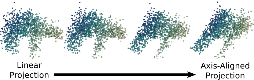
Figure 5: Animation projection transition from a linear projection to one of its constituent axis-aligned projections. As we can observe from the transition, the structure of the linear projection is well preserved in the axis-aligned one, which can be easily explained using the chosen variables.

Projection Transition View. The projection transition view (Figure Exploring High-Dimensional Structure via Axis-Aligned Decomposition of Linear Projections(b)) illustrates the point-wise correspondence between the linear and the axis-aligned projections through an animated transition between them. The starting and ending points for the animation are always defined by linear subspaces (axis-aligned is a special case of linear subspace). Consequently, in order to generate a meaningful transition, it is important to ensure that every frame in the animation corresponds to a valid, linear projection. In this work, we utilize a linear projection matrix interpolation technique, similar to the one discussed in [BCAH97].

Ultimately, we hope to utilize such a transition to connect the qualitative insights we gain from the axis-aligned projections with the structure captured in the linear projection. As illustrated in Figure 5, as we can see the two elongated clusters in the linear projection corresponds to a similar structure in the axis-aligned projection that can be explained by two variables.

Precision-Recall Measure. In order to provide an independent measure of accuracy to validate the quality of any 2D projections, we employ a per-point precision-recall based measure (Figure 4(c)). The concept of precision and recall are widely used in information retrieval and machine learning to evaluate false negative and false positive errors. While being independent of the optimization objective, this provides a natural trade-off between precision and recall metrics, which are both crucial for information visualization [VPN^∗10]. In our visualization, we measure precision and recall of the preserved neighborhood for each data point in the projection with respect to the high dimensional data. We define the neighborhoods for a point $i$ in the original data and the visualization domain as, $\mathcal{N}_{k}(i)$, and $\mathcal{N}^{\prime}_{k^{\prime}}(i)$ respectively where $k$ and $k^{\prime}$ denote the number of points in the neighborhood. The precision and recall values are then computed as, $\text{Precision}=\frac{|\mathcal{N}_{k}(i)\cap\mathcal{N}^{\prime}_{k^{\prime}}(i)|}{k^{\prime}},$ $\text{Recall}=\frac{|\mathcal{N}_{k}(i)\cap\mathcal{N}^{\prime}_{k^{\prime}}(i)|}{k}$. For a given $k$ and $k^{\prime}$ we estimate $\text{fidelity}=0.5*\text{Precision}+0.5*\text{Recall}$. For all results in this paper, we fixed both $k$ and $k^{\prime}$ at $30$.

6 Case Studies

In the following sections, we apply the proposed technique to several real word datasets to illustrate its effectiveness in capturing and explaining structures in linear projections via their axis-aligned decompositions. The examples include both labeled and unlabeled data, with dimension ranging between $7$ and $74$.

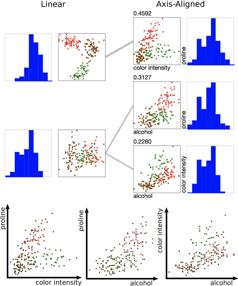
Figure 6: UCI Wine dataset. The red, brown and green classes correspond to three types of wines. The axis-aligned projections clearly illustrate which dimensions produce a class separation structure similar to the one observed in the diverse linear projections obtained with the LDE objective.

6.1 Wine Dataset

The UCI wine dataset is a commonly used dataset for testing classification techniques. The data consists of 13 attributes describing the characteristics of three types of wines (different cultivars). The data has a well-defined class structure, therefore, finding a good linear projection to reveal the class separation is not a particularly challenging task. However, due to the complex linear combination of the projection bases, interpreting the separation structure in terms of individual data dimensions can be difficult. Here, we illustrate how the proposed tool helps to address this challenge via the axis-aligned decomposition of the linear projections.

By utilizing the class separation objective from Local Discriminant Embedding (LDE) (see Table 1), as illustrated in Figure 6, we identify two linear projections that are sufficiently different, yet still reasonably preserve the inherent class structure. As we can see in the first linear projection, the three classes are well separated (highlighted by red, brown, green). However, when examining the actual basis vectors of the projection, they are dense with many active dimensions with similar coefficients. As a result, even though the user can clearly see the structure in the linear projection, it is almost impossible to determine which attribute contributes to the class separation pattern. By augmenting the linear projections with the relevant axis-aligned ones, our tool provides a more intuitive view of the data. In particular, as illustrated in Figure 6, the axis-aligned projections from the decomposition captures similar class separation patterns. More specifically, we observe that the three axis-aligned projections are formed by the attributes color intensity, alcohol, and proline, which directly contribute to the class separation structure. Interestingly, the three attributes also define a 3D subspace where the clusters are cleanly separated.

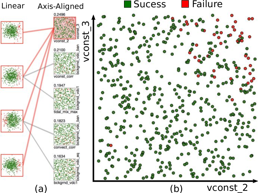
Figure 7: Climate Simulation Run Crashes. The red points correspond to the simulation crashes, and the green ones correspond to successful runs.

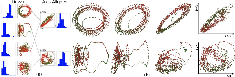
Figure 8: Seawater temperature forecasting dataset. The first axis-aligned projection captures the dominant periodic structure, while the second one highlights an additional loop that is different from one observed in the first projection.

6.2 Climate Simulation Crashes Dataset

An increasingly common approach to study the variability uncertainty inherent in different climate models is to compute large ensembles of simulations with varying input parameters. However, these studies often include parameter combinations that are not well tested or may even be inconsistent with each other. As a result, it is not uncommon for the simulation to fail for a subset of runs. In this situation, it is important to diagnose what parameter (combinations) are involved in a crash to guide the debugging. Here we use a dataset which records successes and failures encountered during simulations of the CCSM4 climate model [LKT^∗13]. The ensemble consists of 18 input parameters and $540$ latin hypercube samples $46$ of which correspond to failures. The objective of the study is to find the relationship between the parameter combinations and failure cases, which can help determine the potential cause for the simulation crashes.

As illustrated in Figure 7(a), we utilize the LDE class separation objective to produce the four representative linear projections, in which the success and failure cases are clearly separated. However, as before it is difficult to determine exactly which dimensions contribute most to separating the success cases from failure cases. We decompose these linear projections to verify if we can obtain a meaningful separation in the axis-aligned projections, which can, in turn, reveal the direct impact of parameters on the simulation crashes. As we can observe from the decomposition in Figure 7(a), despite the diversity of the linear projections, we notice that all linear projections are effectively described (evidenced by the edge thickness) by the highest ranked axis-aligned projection. Note that, the ranking order is determined based on the evidence scores obtained as discussed in Section 4.3. The same plot is enlarged in Figure 7(b), which reveals that the combination of high values for the attributes vconst_2, vconst_3 corresponds to all failure cases (except one outlier) colored by red. There is certainly some overlap between red and green regions, which indicates that other factors exist for exactly determining the outcome, thus justifying the need for analyzing additional axis-aligned plots. However, we easily identify the most useful axis-aligned projection from the exhaustive set of $\frac{18\times(18-1)}{2}$ combinations. Furthermore, it indicates that the attributes vconst_2 and vconst_3 attributes require the most attention when trying to figure out the cause of crashes. Consequently, compared to linear projections, the axis-aligned decomposition provides a much more direct and intuitive interpretation of the patterns. Since the selection of the axis-aligned projections is based on neighborhood structure preservation, the other axis-aligned projections are selected due to their usefulness in preserving the information about the success cases, even though they do not reveal the class separation structure. The ability to produce such complementary structure is the crucial aspect of our approach.

6.3 Seawater Temperature Forecasting Dataset

Time-series analysis and forecasting are required in many applications, and in particular, long term prediction is very challenging. For this experiment, we consider the sea water temperature forecasting dataset [LL07], which is a time series of weekly temperature measurements of sea water over several years. Each data point is a time window of 52 weeks, which is shifted one week forward for the next data point. Altogether there are 823 data points and 52 dimensions. The original goal of this data is to predict the future temperatures based on previous time steps. For this analysis, we hope to identify the repeated pattern, and more interestingly whether or not out-of-ordinary patterns exist in the time series.

Note that, this moving-window representation of a time-series is commonly referred as a delay embedding and is know to reveal periodic structure in the form of loops. The periodic nature is thus very well captured in the first linear projection obtained using LPP based embedding optimization (Figure 8(a)). This projection has high embedding quality when compared to rest of the projections, as indicated by the quality measure histograms and it captures the overall periodic pattern of the data. The corresponding axis-aligned projection, as illustrated in the top row of Figure 8(b), shows a side view of the same pattern. The second linear projection identifies a very interesting pattern. We can notice that there is a second loop, different from the strong loop found in the first linear projection. By viewing the transition from this projection to its corresponding axis-aligned projection, new insights about the structure is revealed. As shown in the bottom row of Figure 8(b), the axis-aligned projection contains an inner loop with most of the samples and an outer loop with a much smaller number of points, thus revealing the presence of two different periodic structures. In another word, our decomposition shows a meaningful separation between the two dominant periodic structures, which is critical information for understanding the complexity of this prediction task.

6.4 NIF Engineering Simulation Dataset

The National Ignition Facility (NIF), a collaboration between Lawrence Livermore, Los Alamos, and Sandia National Laboratories as well as The University of Rochester and General Atomics, is aimed at demonstrating inertial confinement fusion (ICF), that is, thermonuclear ignition and energy gain in a laboratory setting. Fundamentally, the goal of NIF is to search the parameter space to find the region that leads to near-optimal performance, in terms of the energy yield. The dataset considered here is a so-called engineering or macro-physics simulation ensemble in which an implosion is simulated using various different in parameters, such as, laser power, pulse shape etc.. From these simulations scientists extract a set of drivers, physical quantities thought to determine the behavior of the resulting implosion. These drivers are then analyzed with respect to the energy yield to better understand how to optimize future experiments. The dataset, we consider for our the analysis consists of $1304$ samples with $6$ drivers: down scatter fraction (dsf), peak velocity (pv), entropy (sument), (totrhorba), pressure at the centre (prcent), and hotspot radius (hsrad).

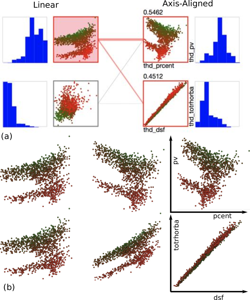
Figure 9: NIF Simulation Data. Our proposed approach reveals the presence of two true clusters in the attribute pv and a strong correlation between the attributes dsf and totrhorba, though the projection artifacts mask the neighborhood structure.

For this exploratory analysis, we choose the LPP objective to find the diverse set of representative linear projections. Figure 9(a) shows the two representative linear projections produced by our approach, and the two axis-aligned projections that describe the structures induced in the linear embeddings. The projection with the highest evidence is comprised of the attributes pv, pcent, which reveals the two elongated protruding clusters. The transition from the linear projection to the {pv, pcent} subspace (top row of Figure 9(b)) illustrates the small structural differences between them. As we can see in the axis-aligned plot, the high/low value of pv roughly corresponds to two protruding clusters. The second highest projection reveals a strong linear correlation between totrhorba and dsf. Interestingly, the precision-recall based quality measure indicates that the second axis-aligned projection contains significantly more artifacts than the first one, yet the evidence measure claims both axis-aligned projections capture important structures. To help explain the cause of the projection error, we apply a transition between the two projections (bottom row of Figure 9(b)). Here we notice that the two clusters in the original linear projection become overlapped while transitioning to the {totrhorba,hsrad} plot. Consequently, we infer that there are two geometrically distinct regions in the high-dimensional space where the attributes totrhorba, dsf are strongly correlated. Due to the overlap in the axis-aligned projection, the neighborhood structure is partially lost (as indicated by the histogram of the quality). Nevertheless, our algorithm is able to correctly determine that this relationship is valid and assigns a high evidence score.

Consulting with the relevant physicists, we have confirmed that the correlation observed between the two attributes agrees with the underlying physics. More importantly, the axis-aligned projection that captures the two protruding clusters in the linear projection are very useful, since that structure is inherently more challenging to interpret in a linear projection as stated by the physicists in a previous study (part of the motivation for this work).

7 Discussion

This work introduced a novel algorithm for decomposing structure-preserving linear projections into a compact set of interpretable axis-aligned scatterplots. Combined with a novel optimization technique for generating representative linear projections and an intuitive visual interface, we allow users to explore complex high-dimensional data and make connections between the observed structure (e.g., clusters, correlations) and the actual data dimensions. By jointly examining the structure preservation effectiveness of linear projections via the quality measure histograms and the evidence of the axis-aligned plots via the edge thicknesses in the relationship view, the users can obtain a good understanding of how much of the inherent high-dimensional structure can be explained by the data dimensions.

As demonstrated by our case studies, the proposed method is widely applicable to a broad range of unsupervised and supervised analysis tasks. A potential limitation of this approach is that the axis-aligned plots are not easily comparable to their corresponding linear projections, when the attributes are categorical (binary or multiple states) in nature. In our case studies, we are dropping the categorical variables out of the analysis, if they exist. Due to the efficiency of the proposed algorithm, our method can adapt to both very high dimensions (>100), as well as large sample size (>10000). The dominant complexity of the linear projection finding step arises from the generalized eigenvalue decomposition of the matrices of size $d\times d$, where $d$ is the number of dimensions. On the other hand, the greedy algorithm for performing the decomposition incurs a complexity of order $\mathcal{O}(dn)$, where $n$ is the total number of samples.

References

- [Asi85] Asimov D.: The grand tour: a tool for viewing multidimensional data. SIAM journal on scientific and statistical computing 6, 1 (1985), 128–143.
- [AW10] Abdi H., Williams L. J.: Principal component analysis. Wiley interdisciplinary reviews: computational statistics 2, 4 (2010), 433–459.
- [BCAH97] BUJA A., COOK D., ASIMOV D., HURLEY C.: Theory and computational methods for dynamic projections in high-dimensional data visualization. Journal of computational and graphical statistics (1997).
- [BTK11] Bertini E., Tatu A., Keim D.: Quality metrics in high-dimensional data visualization: An overview and systematization. IEEE Transactions on Visualization and Computer Graphics 17, 12 (2011), 2203–2212.
- [CBC93] Cook D., Buja A., Cabrera J.: Projection pursuit indexes based on orthonormal function expansions. Journal of Computational and Graphical Statistics 2, 3 (1993), 225–250.
- [CCL05] Chen H.-T., Chang H.-W., Liu T.-L.: Local discriminant embedding and its variants. In Computer Vision and Pattern Recognition, 2005. CVPR 2005. IEEE Computer Society Conference on (2005), vol. 2, IEEE, pp. 846–853.
- [CG05] Chipman H. A., Gu H.: Interpretable dimension reduction. Journal of applied statistics 32, 9 (2005), 969–987.
- [DD14] Dadkhahi H., Duarte M. F.: Masking schemes for image manifolds. In Statistical Signal Processing (SSP), 2014 IEEE Workshop on (2014), IEEE, pp. 252–255.
- [FT74] Friedman J. H., Tukey J. W.: A projection pursuit algorithm for exploratory data analysis.
- [HSSL13] Harandi M., Sanderson C., Shen C., Lovell B. C.: Dictionary learning and sparse coding on grassmann manifolds: An extrinsic solution. In Computer Vision (ICCV), 2013 IEEE International Conference on (2013), IEEE, pp. 3120–3127.
- [KW78] Kruskal J. B., Wish M.: Multidimensional scaling, vol. 11. Sage, 1978.
- [LBJ∗16] Liu S., Bremer P.-T., Jayaraman J., Wang B., Summa B., Pascucci V.: The grassmannian atlas: A general framework for exploring linear projections of high-dimensional data. In Computer Graphics Forum (2016), vol. 35, Wiley Online Library, pp. 1–10.
- [LKT∗13] Lucas D., Klein R., Tannahill J., Ivanova D., Brandon S., Domyancic D., Zhang Y.: Failure analysis of parameter-induced simulation crashes in climate models. Geoscientific Model Development 6, 4 (2013), 1157–1171.
- [LL07] Lendasse A., Liitiainen E.: Variable scaling for time series prediction: Application to the ESTSP’07 and the NN3 forecasting competitions. In IJCN (Aug 2007).
- [LMW∗17] Liu S., Maljovec D., Wang B., Bremer P.-T., Pascucci V.: Visualizing high-dimensional data: Advances in the past decade. IEEE transactions on visualization and computer graphics 23, 3 (2017), 1249–1268.
- [LT16] Lehmann D. J., Theisel H.: Optimal sets of projections of high-dimensional data. Visualization and Computer Graphics, IEEE Transactions on 22, 1 (2016), 609–618.
- [LWT∗15] Liu S., Wang B., Thiagarajan J. J., Bremer P.-T., Pascucci V.: Visual exploration of high-dimensional data through subspace analysis and dynamic projections. In Computer Graphics Forum (2015), vol. 34, Wiley Online Library, pp. 271–280.
- [MH08] Maaten L. v. d., Hinton G.: Visualizing data using t-sne. Journal of Machine Learning Research 9, Nov (2008), 2579–2605.
- [Mor92] Morton S. C.: Interpretable exploratory projection pursuit. In Computing Science and Statistics. Springer, 1992, pp. 470–474.
- [MRW∗99] Mika S., Ratsch G., Weston J., Scholkopf B., Mullers K.-R.: Fisher discriminant analysis with kernels. In Neural Networks for Signal Processing IX, 1999. Proceedings of the 1999 IEEE Signal Processing Society Workshop. (1999), IEEE, pp. 41–48.
- [Niy04] Niyogi X.: Locality preserving projections. In Neural information processing systems (2004), vol. 16, MIT, p. 153.
- [NM13] Nam J. E., Mueller K.: Tripadvisor^ND: A tourism-inspired high-dimensional space exploration framework with overview and detail. IEEE transactions on visualization and computer graphics 19, 2 (2013), 291–305.
- [S∗76] Shafer G., et al.: A mathematical theory of evidence, vol. 1. Princeton university press Princeton, 1976.
- [SS04] Seo J., Shneiderman B.: A rank-by-feature framework for unsupervised multidimensional data exploration using low dimensional projections. In Information Visualization, 2004. INFOVIS 2004. IEEE Symposium on (2004), IEEE, pp. 65–72.
- [TG07] Tropp J. A., Gilbert A. C.: Signal recovery from random measurements via orthogonal matching pursuit. IEEE Transactions on information theory 53, 12 (2007), 4655–4666.
- [TMF∗12] Tatu A., Maass F., Färber I., Bertini E., Schreck T., Seidl T., Keim D. A.: Subspace search and visualization to make sense of alternative clusterings in high-dimensional data. In IEEE VAST (2012), IEEE Computer Society, pp. 63–72.
- [Tuk80] Tukey J. W.: We need both exploratory and confirmatory. The American Statistician 34, 1 (1980), 23–25.
- [VPN∗10] Venna J., Peltonen J., Nybo K., Aidos H., Kaski S.: Information retrieval perspective to nonlinear dimensionality reduction for data visualization. Journal of Machine Learning Research 11, Feb (2010), 451–490.
- [WAG05] Wilkinson L., Anand A., Grossman R. L.: Graph-theoretic scagnostics. In INFOVIS (2005), vol. 5, p. 21.
- [WM17] Wang B., Mueller K.: The subspace voyager: Exploring high-dimensional data along a continuum of salient 3d subspace. IEEE Transactions on Visualization and Computer Graphics (2017).
- [YL14] Ye K., Lim L.-H.: Distance between subspaces of different dimensions. arXiv preprint arXiv:1407.0900 (2014).
- [YRWG13] Yuan X., Ren D., Wang Z., Guo C.: Dimension projection matrix/tree: Interactive subspace visual exploration and analysis of high dimensional data. IEEE Transactions on Visualization and Computer Graphics 19, 12 (2013), 2625–2633.
- [YXZ∗07] Yan S., Xu D., Zhang B., j. Zhang H., Yang Q., Lin S.: Graph embedding and extensions: A general framework for dimensionality reduction. IEEE Transactions on Pattern Analysis and Machine Intelligence 29, 1 (Jan 2007), 40–51. doi:10.1109/TPAMI.2007.250598.