Dynamics of Tunneling Ionization using Bohmian Mechanics

Abstract

Recent attoclock experiments and theoretical studies regarding the strong-field ionization of atoms by few-cycle infrared pulses revealed new features that have attracted much attention. Here we investigate tunneling ionization and the dynamics of the electron probability using Bohmian Mechanics. We consider a one-dimensional problem to illustrate the underlying mechanisms of the ionization process. It is revealed that in the major part of the below-the-barrier ionization regime, in an intense and short infrared pulse, the electron does not tunnel “through” the entire barrier, but rather already starts from the classically forbidden region. Moreover, we highlight the correspondence between the probability of locating the electron at a particular initial position and its asymptotic momentum. Bohmian Mechanics also provides a natural definition of mean tunneling time and exit position, taking account of the time dependence of the barrier. Finally, we find that the electron can exit the barrier with significant kinetic energy, thereby corroborating the results of a recent study [Camus et al., Phys. Rev. Lett. 119 (2017) 023201].

I Introduction

The tunneling ionization of an electron in an ultra-short intense optical laser pulse represents a purely quantum process whose theoretical description remains challenging. Numerous treatments, based on various approximations, have been elaborated to model ionization in the tunneling regime, e.g., using the adiabatic theorem Joachain00 , the strong-field approximation (SFA) Keldysh65 ; Faisal73 ; Reiss80 , the closed-orbit theory Du87 , the simple-man’s model Corkum89 , as well as more recent techniques Klaiber15 ; Yakaboylu14 ; Torlina12 ; Torlina14 . Although these models can already make impressive predictions, the ultrafast electron dynamics in a time-varying barrier remains a process under great scrutiny that has been triggering extensive theoretical work. Improving our understanding of tunneling ionization is crucial for high-order harmonic generation (HHG), coherent quantum control, and attosecond science in general.

The present study is devoted to a description of tunneling ionization employing Bohmian Mechanics Bohm52 ; Durr09 ; Botheron10 , which has recently attracted much attention Zimmermann16 ; Steinberg11 ; Braverman13 ; Steinberg16 ; Ivanov17 ; Song17 ; Benseny14 ; Jooya1 ; Jooya2 ; Jooya3 ; Jooya4 . It will be shown that computing the streamlines of the wavefunction probability over time provides valuable insights and a natural route to understanding complex ultrafast mechanisms. Despite the fact that Bohmian Mechanics leads to the same final results as Quantum Mechanics, it offers an alternative route to the complex time evolution of a wavepacket by considering the streamlines of the electron probability over time while going beyond the SFA. Relating the wavefunction dynamics to particle trajectories, as for instance done in the Feynman path integral approach or in semiclassical models, represents a very appealing aspect of Bohmian Mechanics.

An important topic to which Bohmian Mechanics can make a unique contribution concerns the understanding of “tunneling time” through a potential barrier, as recently considered in Ref. Zimmermann16 . The concept of tunneling time (e.g., Larmor Buttiker83 , Büttiker-Landauer Buttiker82 , Pollack-Miller Pollack84 , or Eisenbud-Wigner times Wigner55 ) is a fuzzy concept, as it cannot be obtained directly from a physical observable. Since the various definitions lead to different results Landsman14 ; Zimmermann16 , one might even question the relevance of a tunneling time. On the other hand, the concept plays a central role in the Keldysh theory Keldysh65 , since it provides a criterion to separate the multiphoton and the tunneling ionization regimes.

Revisiting the concept of tunneling time has become highly appropriate with the advent of attoclock experiments Landsman14 ; Camus17 and debates around the claim of Torlina et al. Torlina15 that optical tunneling in atomic hydrogen is instantaneous. Indeed, two recent studies Ni16 ; Sainadh17 obtained results supporting a tunneling ionization time close to zero, while others Landsman14 ; Zimmermann16 ; Camus17 reported a nonzero tunneling time for traversing the barrier. Note that the tunneling ionization time defined in Torlina15 ; Ni16 corresponds to the moment at which the electron appears at the tunnel exit with respect to the instant of maximum field strength, and thus it does not necessarily contradict the results of Refs. Landsman14 ; Zimmermann16 . One might also suggest that part of the disagreement observed between different studies is due to electron correlations in multielectron systems. However, the recent work by Majety and Scrinzi Majety17 on helium revealed that electron correlations should have no effect on the asymptotic electron momentum offset angle.

In this study, we show that Bohmian Mechanics provides natural definitions of tunneling ionization time, traversing time, and exit points for each trajectory, while explicitly accounting for the barrier dynamics. Bohmian Mechanics can provide a picture of the time propagation under a barrier without invoking imaginary tunneling time. Bohmian Mechanics might thus have the potential to reveal and rationalize the dynamics above and below a barrier, while only using familiar concepts.

In order to establish the basic ideas, we consider a one-dimensional model problem, which contains the principal ingredients of the tunneling process without adding nonessential complexities. The study is thus not intended as a direct application to a current experimental problem, but as the presentation of an alternative approach with attractive characteristics for application in ultrafast physics, with the perspective that a similar approach could be performed on a realistic case. Specifically, it will be shown that even for the one-dimensional problem considered in this work, Bohmian Mechanics provides important physical results that can hopefully be transferred to the real case.

Specifically, we demonstrate that the major part of below-the-barrier-ionization (BBI) induced by an intense ultrashort infrared pulse originates from the electron probability initially located inside the classically forbidden region, i.e., from the tail of the initial ground-state wavefunction. Hence the picture of the probability flow traversing the entire barrier from the inner to the outer classically allowed regions is fundamentally flawed. Furthermore, we show that an above-threshold ionization (ATI) photoelectron spectrum can be accurately reproduced through Bohmian Mechanics, thus leading to an appealing correspondence between the total number of absorbed photons and the initial probability distribution of the electron position. Bohmian Mechanics also provides indications on when the quantum effects become negligible, i.e., when the so-called “quantum force” Bohm52 ; Durr09 vanishes. As a result, a particle emerging from the barrier can still exhibit quantum behavior for a significant time.

This manuscript is organized as follows: In the next section II, we outline the theoretical approach and describe the model considered. Our results are presented and discussed in Sec. III, where we consider Bohmian trajectories, their correspondence to the final quantum photoelectron ionization spectrum, and how they can be used to define tunneling time and exit position. Section IV summarizes our conclusions.

Unless stated otherwise, atomic units are used throughout the manuscript.

II Theoretical approach

Suppose $\varphi(x,t)=R(x,t)\exp{\left[iS(x,t)\right]}$,with $R$ and $S$ being real-valued functions, is the solution of the time-dependent Schrödinger Equation (TDSE). In Bohmian Mechanics in one dimension, electron trajectories are computed from the following set of equations Bohm52 ; Ivanov17 :

$$-\frac{\partial S(x,t)}{\partial t} \!=\! \frac{1}{2}\left(\frac{\partial S(x,t)}{\partial x}\right)^{2}\!\!\!+V_{C}(x,t)\!+\!V_{Q}(x,t);$$ (1)

$$\frac{\partial\rho(x,t)}{\partial t} \!=\! -\nabla\cdot[{\rho(x,t)v(x,t)}].$$ (2)

Here $\rho(x,t)=R(x,t)^{2}$ is the probability density and $v(x,t)=\Re\{[\hat{p}\,\varphi(r,t)]/\varphi(r,t)\}$ is the velocity field, where $\Re\{X\}$ denotes the real part of $X$ and $\hat{p}$ the momentum operator. Furthermore, $V_{C}(x,t)$ and $V_{Q}(x,t)=-0.5\Delta R(x,t)/R(x,t)$ are the classical and quantum potentials, respectively. Equation (1) is the Hamilton-Jacobi equation with the addition of the quantum potential $V_{Q}(x,t)$ Riggs07 , while Eq. (2) is the continuity equation for a current probability density $j(x,t)=\rho(x,t)v(x,t)$. Equations (1) and (2) are formally equivalent to the TDSE.

After evaluating the velocity field $v(x,t)$ from the solution $\varphi(x,t)$ of the TDSE, we integrate the equation $dx(t)/dt=v(x,t)$, starting from an initial position $x(x_{0};0)=x_{0}$ at $t=0$, to compute classical trajectories $x(x_{0};t)$ of the probability streamlines. [Note that we maintain the commonly-used notation here, even though the time-dependent position $x(t)$ is not the same as the spatial grid on which the various functions are defined.] These Bohmian trajectories have a broader significance than classical trajectories and can, for instance, be used to reconstruct the wavefunction at any time Botheron10 ; Schleich13 . Very importantly, the quantum potential allows Bohmian trajectories to penetrate into classically forbidden regions.

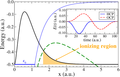
Figure 1: Representation of the ground-state probability (thick black line), the field-free Yukawa potential (thin blue line), and the classical potential at the maximum field strength (dashed green line) for $I_{0}=4\times 10^{14}~{}$W/cm². The insert shows the electric fields of our HCP and OCP (see text for details).

We consider a one-dimensional model, $x\in[-\infty,+\infty]$, and use, as our principal example, a short-range Yukawa potential $V_{0}(x)=-Z\exp(-|x|)/|x|$, truncated at $\varepsilon=0.01$, such that $V_{0}(x)=V_{0}(\varepsilon)$ for $|x|<\varepsilon$. This potential was also used in Abramovici09 . It could, for instance, model the photodetachment of an atomic anion. We also carried out calculations for a truncated Coulomb potential, i.e., a one-dimensional H atom, and we discuss some of these results below.

Due to its illustrative advantages and regular behavior Abramovici09 , we consider the initial wavefunction $\varphi_{0}(x)$ to be the odd-parity eigenstate of lowest energy. For $x\geq 0$, therefore, $\varphi_{0}(x)$ is the (reduced) radial part of the $1s$ ground state of the corresponding three-dimensional problem. We set $Z=-1.9083$ to produce an energy of $\varepsilon_{0}=-0.5~{}$.

The electric field $E(t)=E_{0}f(t)\sin(\omega t+\phi)$ has amplitude $E_{0}$, frequency $\omega=0.05811$ ($\lambda=784$ nm), phase $\phi$, and a sine-squared envelope $f(t)=\sin^{2}(\Omega t)$, where $\Omega=\omega/2N$ with $N$ as the number of cycles. The TDSE is solved in the length gauge, with $V_{C}(x,t)=V_{0}(x)+E(t)x$, by a finite-difference method.

Throughout this study, we mostly consider a half-cycle pulse (HCP) with $\phi=180^{\circ}$, so that the electron is pulled towards the positive direction. This represents the simplest case to illustrate the essence of the BBI process. We choose a peak intensity $I_{0}=4\times 10^{14}$ W/cm² to remain relatively far from over-the-barrier ionization (OBI) starting at $I_{\rm OBI}=1.2\times 10^{15}$ W/cm². We also consider a one-cycle pulse (OCP) carrying the same energy as the HCP, i.e., with $I_{0}\approx 1.68\times 10^{14}{\rm W/cm}^{2}$ and $\phi=0^{\circ}$. The Yukawa potential, $V_{0}(x)$, and the classical potential at the maximum field strength are plotted for $x\geq 0$ in Fig. 1.

III Results and discussion

III.1 Bohmian dynamics

Having obtained the numerical solution of the TDSE, we computed thousands of trajectories using the Runge-Kutta method NumRep , starting from rest ($j(x,0)=0$) at initial positions $x_{0}$. A few of these trajectories, plotted in Fig. 2 (a), exhibit a smooth variation without apparent interference between paths. This simple situation contrasts with the cases of a few-cycle pulse Botheron10 , as well as the well-known example of entangled trajectories in the double-slit problem with photons Steinberg11 .

A rich amount of information can be extracted from the Bohmian trajectories. First, we found that only trajectories starting in the “ionizing region” defined by $x_{0}\geq x_{\rm th}$ become asymptotically free, i.e., with a final speed $v_{\infty}>0$. As seen in Fig. 1, this ionizing region is located inside the classically forbidden region. It starts at $x_{\rm th}=1.65$ a.u., whereas the inner turning point for the energy $\varepsilon_{0}$ is $x_{\rm cl}=1.17~{}{\rm a.u.}$. At the lower intensity of $I_{0}=2\times 10^{14}~{}$W/cm², $x_{\rm th}=2.70$ a.u., deep inside the forbidden region, while $x_{\rm th}=x_{\rm cl}$ near $I_{0}\approx 6\times 10^{14}~{}$W/cm². Consequently, only for intensities close to the OBI regime, part of the tunneling can be considered as occurring across the barrier.

Even though the characteristics of the ionizing region depend on the exact form of the pulse and potential, the latter trend survives for a Coulomb potential and a OCP. Given that OBI occurs at $I_{\rm OBI}=1.5\times 10^{14}~{}$W/cm² in atomic hydrogen, $x_{\rm th}=2.2$ at $I_{0}=10^{14}~{}$W/cm² while $x_{\rm cl}=2.0$. For the OCP, the ionizing region exists for $|x_{0}|$ above a certain threshold, which is different for $x\geq 0$ and $x<0$.

We then repeated the calculations for 2- and 3-cycle pulses and confirmed these general findings. The trend is expected to also hold in three dimensions, which would confirm the conclusion expressed in Ref. Khausal17 , namely: In a specific ionization regime, tunneling only occurs from the tail of the initial wavefunction.

In order to understand the tunneling dynamics, it is instructive to look at the acceleration $\ddot{x}(x_{0};t)$ of the trajectories as a function of time. Figure 2 (b) shows the acceleration of a few asymptotically free trajectories, as well as the electric force $F_{\rm e}(t)$ created by the HCP. Not surprisingly, the acceleration approaches $F_{\rm e}(t)$ with increasing time, and the acceleration for small initial positions $x_{0}$ merges the latter onto the electric force. The discrepancy between the acceleration and $F_{\rm e}(t)$ is partly due to the Yukawa force $F_{0}(x)=-dV_{0}(x)/dx$, but also to the quantum force $F_{Q}(x,t)=-\partial V_{Q}(x,t)/\partial x$. Initially, $F_{Q}(x,0)=-F_{0}(x)$, since the system is in equilibrium at zero field. For trajectories starting at large $x_{0}$, $F_{0}(x)$ becomes rapidly negligible in comparison with $F_{Q}(x,t)$ due to the short-range nature of the potential. The quantum force $F_{Q}(x,t)$ provides the extra energy that, in conjunction with the field energy, allows the particle to cross the barrier and emerge into the classically allowed region. It is also interesting to note the counterintuitive fact that some trajectories, while still under the barrier, can experience an acceleration greater than that of a particle in the electric field only.

After the acceleration curve merges onto the electric force, the trajectory is the one of a classical particle interacting with the field only. This can, of course, only occur after the particle has emerged from the classically forbidden region. We also repeated the same calculations using a longer wavelength ($\lambda=1568$ nm) and found the same general behavior, although trajectories merge more smoothly onto the electric force due to the slower variations of the barrier. For the Coulomb case, the particle starts behaving classically as soon as the acceleration merges onto the force $F_{C}(x,t)=-\partial V_{C}(x,t)/\partial x$, which includes the long-range Coulomb force.

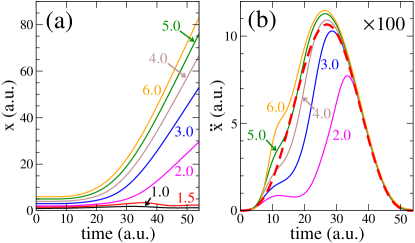
Figure 2: (Color online) Bohmian trajectories (a) and associated acceleration (b) as a function of time labeled by their initial position $x_{0}$. The dashed red curve represents the time-dependent electric force $F_{\rm e}(t)=-E(t)$.

We also performed calculations using the OCP. The dynamics is slightly more complicated (not shown), and the quantum effects more pronounced, as the electron experiences a force oriented alternatively in each direction. The overall conclusions, however, remain the same. The ionization occurs predominantly along the positive direction, as several trajectories driven by the first maximum of the OCP towards $x<0$ rescatter towards the origin. Many of these rescattering trajectories are thrown back at the end of the pulse towards the negative direction by the quantum force, while other trajectories recombine in the attractive region, perturbing bound orbits, and inducing an ionization burst towards $x>0$. This effect is due in part to the fact that Bohmian trajectories cannot cross.

$\begin{array}[]{c}\vspace{-0.55cm}\includegraphics[width=195.12767pt]{Fig3a.pdf}\\ \includegraphics[width=195.12767pt]{Fig3b.pdf}\end{array}$

Figure 3: Ionization spectra for the HCP (a) and OCP (b) pulses calculated using quantum (solid black line) and Bohmian (dashed red line) Mechanics. The insets show the wavefunction probability at the end of each pulse. The shaded regions give the corresponding interval of initial positions (see text for details).

The photoelectron spectrum represents a very important measurable quantity in SFI. One additional advantage of Bohmian Mechanics is that the distribution of asymptotic speeds $v_{\infty}$ of ionized trajectories has the same density distribution $\left|\hat{\varphi}(p)\right|^{2}$ as in standard Quantum Mechanics Durr09 . Here $p=v_{\infty}$, and $\hat{\varphi}$ is the Fourier transform of the wavefunction at $t\to\infty$. Hence, we computed the differential ionization probability $\Delta{\cal P}/\Delta\varepsilon=\Delta x_{0}\left|\varphi(x_{0},0)\right|^{2}/\Delta\varepsilon$, with $\varepsilon=v_{\infty}^{2}/2$ being the asymptotic energy of a trajectory starting at $x_{0}$, and $\Delta\varepsilon$ the energy difference between nearby trajectories starting at $x_{0}$ and $x_{0}+\Delta x_{0}$, respectively.

To illustrate the ideas, we present the ionization probability associated with positive asymptotic momenta. The results obtained in both Bohmian and quantum approaches are plotted for both pulses in Fig. 3 and show nearly perfect agreement. One can thus establish a correspondence between the initial electron position, the region of space to where the electron has probabilistically evolved at any time, and the region of the ionization spectrum that its asymptotic energy will cover.

The correspondence is illustrated in Fig. 3, where we partitioned the ionization spectrum with the associated range of initial positions, and with the electron probability density at the end of the pulse. The areas labeled by the initial positions $x_{1}\leq x_{0}\leq x_{2}$ in the spectrum equal the probability $\int^{x(x_{2};t)}_{x(x_{1};t)}\left|\varphi(x,t)\right|^{2}dx$ to find the particle at any given time in this interval, and in particular the total ionization probability ${\cal P}=\int^{\infty}_{x_{\rm th}}\left|\varphi_{0}(x)\right|^{2}dx$. Note, however, that a final momentum can in general be reached through more than one initial position for more complex pulses. For the OCP, the convergence of asymptotic velocities is slower, because there exist more interactions between paths. Each peak of the ATI spectrum can be associated with a range of initial electron positions and the number of absorbed photons. Note that an ATI spectrum presented as histograms with wide energy steps was obtained for a one-dimensional model using Bohmian Mechanics in Lai13 . The agreement with the TDSE spectrum, however, was not nearly as good as the one presented here.

III.2 Tunneling time and exit position

Computing the main electron ejection angle in a single-cycle circularly polarized infrared pulse, Torlina et al. Torlina15 claimed a zero “tunneling ionization time” $\uptau_{\rm ion}$ for an electron bound in a Yukawa or Coulomb potential. The latter time, $\uptau_{\rm ion}=\uptau_{\rm ex}-\uptau_{\rm max}$, is defined with respect to the instant $\uptau_{\rm max}$ of maximum field, and with the exit time $\uptau_{\rm ex}$ from the barrier. Ni et al. Ni16 confirmed a near-zero ionization time using classical backpropagation in a 2D model starting with a local momentum Feuerstein03 ; Wang13 obtained from the solution of the TDSE. They defined the detachment time, when $\bm{p+A}$ has no component along the field direction, as the criterion to exit the barrier. While their study allowed to compute the time at which the electron trajectories tunnel out of the barrier, it provides limited information on the dynamics preceding the tunneling. In addition, a recent study Camus17 showed that the electron escapes the barrier with nonzero longitudinal momentum, thereby contradicting the detachment criterion employed in Ni16 . Zimmermann et al. Zimmermann16 computed the “tunneling” or “traversing time”, i.e., the time spent by the electron under the barrier, using standard definitions Buttiker83 ; Buttiker82 ; Pollack84 ; Wigner55 . Additionally, a Bohmian tunneling time to cross the barrier was computed in the adiabatic approximation using a time-independent outgoing solution of the Schrödinger equation in a static electric field. However, ignoring important aspects, such as the time variation of the barrier, and the fact that most of the ionization does not cross the entire barrier, lead to a drastic overestimation of the Bohmian tunneling time. Below, we show that Bohmian Mechanics provides natural answers to the aspects mentioned above.

The Bohmian approach is well suited to define a tunneling time Leavens90 . In the length gauge, the tunneling condition, which includes nonadiabatic effects, is given by $\varepsilon(t)=V_{C}(x,t)$, with $\varepsilon(t)$ denoting the time-dependent energy of a trajectory. In the classical case, it would correspond to a zero instantaneous speed $v(x)$ of the particle at the exit of the barrier. Note, however, that this represents only an approximate condition, since the semiclassical description breaks down at $v(x)\approx 0$. Tunneling occurs when $\varepsilon(t)<V_{C}(x,t)$. This is forbidden in Classical Mechanics, but allowed for Bohmian trajectories, as long as $\varepsilon(t)\geq V_{C}(x,t)+V_{Q}(x,t)$. The tunneling condition is equivalent to $T=-V_{Q}(x,t)$ ($T$ being the kinetic energy) and tends towards the classical limit for $V_{Q}(x,t)\ll 1$. In stark contrast to the classical case, the Bohmian particle emerges from the barrier with a nonzero velocity.

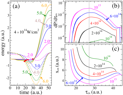
Figure 4: (a) Energy (solid lines) and $V_{C}(x,t)$ (dashed lines) as a function of time for trajectories labeled by their initial positions (the exit times $\uptau_{\rm ex}$ are marked by red dots), (b) probability density $d{\cal P}/d\uptau_{\rm\rm ex}$, and (c) exit point $x_{\rm ex}$ as a function of $\uptau_{\rm ex}$, for several peak intensities (in W/cm²). The vertical dotted line indicates $\uptau_{\rm max}$ (see text for details).

The time-dependent energy $\varepsilon(t)$ and the classical potential $V_{C}(x,t)$ of a few asymptotically free trajectories are presented in Fig. 4 (a) for the HCP at $4\times 10^{14}$ W/cm². All energy curves start at $\varepsilon_{0}$, have a classical asymptotic energy $v_{\infty}^{2}/2$ whose distribution reproduces the quantum spectrum (see Fig. 4(a)), and their energy averaged over all trajectories equals the total energy of the quantum system at any time Song17 . Each energy curve crosses $V_{C}(x,t)$ at $\uptau_{\rm ex}$, and deviations of $\varepsilon(t)$ from $\epsilon_{0}$ at a crossing point are the signature of nonadiabatic effects. Trajectories traveling the furthest out experience the maximum decrease in $V_{C}(x,t)$, followed by the largest increase in $\varepsilon(t)$. At $I_{0}\geq 6\times 10^{14}~{}$W/cm², trajectories with $x_{\rm th}\leq x_{0}\leq x_{\rm cl}$ cross $V_{C}(x,t)$ twice (not shown), as they enter and exit the classically forbidden region at $\uptau_{\rm en}$ and $\uptau_{\rm ex}$, respectively. Fitting $\uptau_{\rm ex}$ and $\uptau_{\rm en}$ as a function of the initial position, we found, approximately, that $\uptau_{\rm ex}\propto(x_{0}-x_{\rm th})^{-0.2}$ and $\uptau_{en}\propto(x_{cl}-x_{0})^{0.3}$ for $x_{\rm th}\leq x_{0}\leq x_{\rm cl}$ at all intensities studied. As expected, $\uptau_{\rm ex}\gg 1$ when $x_{0}\approx x_{\rm th}$, while $\uptau_{\rm en}$ increases suddenly when $x_{0}$ enters the classically allowed region. Thus, trajectories with $x_{0}<x_{\rm cl}$ spend a long time inside the allowed region before entering the barrier.

Comparing the results of Figs. 2 (a) and 4, we see that some trajectories become classical only a significant time after tunneling. For example, the trajectory with initial position $x_{0}=6.0$ exits the barrier at $\uptau_{\rm ex}\approx 20$ a.u. while it becomes classical only after 30 a.u.. Moreover, in Bohmian Mechanics, the particle naturally emerges from the barrier with a nonzero kinetic energy $T_{\rm ex}$. In the three-dimensional case, Bohmian trajectories would exit the barrier with a nonvanishing longitudinal momentum. This is in agreement with recent findings Camus17 , but departs from the common assumption used in both the SFA and Ref. Ni16 . Table 1 summarizes the characteristics of Bohmian trajectories for different initial positions.

The differential ionization probability $d{\cal P}/d\uptau_{\rm ex}$ for trajectories exiting at $\uptau_{\rm ex}$ is presented in Fig. 4 (b) for several peak intensities. The maximum exit time increases with intensity and $d{\cal P}/d\uptau_{\rm ex}$ drops sharply at large $\uptau_{\rm ex}$. The most probable exit time is larger than the instant of maximum field strength ($\uptau_{\rm max}\approx 27$ a.u.) at all intensities, but tends towards $\uptau_{\rm max}$ with increasing intensity (the difference is $\leq 0.2$ a.u. at $1.1\times 10^{15}~{}$W/cm²). The fact that $d{\cal P}/d\uptau_{\rm ex}$ exhibits a broad maximum and flat regions is due to the sin² envelope. The maximum would appear sharper and better defined for a narrower envelope.

$x_{0}$	$\uptau_{\rm ex}$	$x_{\rm ex}$	$T_{\rm ex}$
$1.7$	35.86	$5.18$	$0.050$
$2.0$	29.40	$4.78$	$0.073$
$3.0$	23.23	$5.55$	$0.096$
$4.0$	20.79	$6.63$	$0.126$
$5.0$	19.59	$7.79$	$0.159$
$6.0$	18.87	$9.00$	$0.191$

Table 1: Exit time $\uptau_{\rm ex}$, position $x_{\rm ex}$, and kinetic energy $T_{\rm ex}$ of Bohmian trajectories with different initial positions for $I_{0}=4\times 10^{14}$W/cm². All values are given in a.u..

Fig. 4 (c) shows the exit position $x_{\rm ex}$ from the barrier, as a function of the exit time $\uptau_{\rm ex}$, for different intensities. The trajectories escaping the barrier the fastest have the largest exit position, since the barrier remains broad far from $\uptau_{\rm max}$. All curves, except for 10¹⁴ W/cm², exhibit a minimum corresponding to escape when the barrier is the thinnest. Its position is slightly shifted from the most probable exit time and also tends towards $\uptau_{\rm max}$ with increasing intensity. The absence of a minimum at $10^{14}~{}$W/cm² is due to strong nonadiabatic effects, which allow trajectories to leave with $\varepsilon(t)$ significantly larger than $\varepsilon_{0}$, and hence with an exit position smaller than the adiabatic instantaneous turning point at the maximum field strength ($\approx 9.4$ a.u.). In fact, the energy $\varepsilon(t)$ of trajectories escaping with the minimum value of $x_{\rm ex}$ tends to decrease with intensity, such that $x_{\rm ex}$ becomes larger than the adiabatic value for $I_{0}\geq 6\times 10^{14}~{}$W/cm².

The mean values $\bar{\uptau}_{\rm ion}$ and $\bar{\uptau}_{\rm tra}$ are presented in Fig. 5, where $\uptau_{\rm tra}=\uptau_{\rm ex}-\uptau_{\rm en}$ is the traversing time through the barrier. At the intensities studied, $\bar{\uptau}_{\rm ion}$ is relatively small and decreases towards zero as the intensity gets closer to the OBI regime. The variation of $\bar{\uptau}_{\rm ion}$ resembles the experimental tunneling time in Landsman14 . In contrast to the results of Zimmermann et al. Zimmermann16 who used time-independent functions, $\bar{\uptau}_{\rm ex}$ does not become orders of magnitude larger at low intensities.

It turns out that the traversing time shown in Fig. 5 is a shift of $\bar{\uptau}_{\rm ion}$ by $\uptau_{\rm max}$ (note the different scales in the panels of Fig. 5) until the peak intensity reaches $6\times 10^{14}$ W/cm². The observed inflection point is due to contributions from probability located in the inner classical region. These take a long time to reach the barrier, but they enter it with a nonnegligible kinetic energy, thereby causing the traversing time to decrease faster.

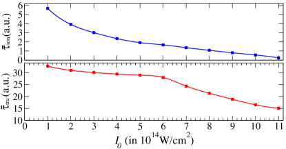
Figure 5: Mean tunneling ionization time $\bar{\uptau}_{\rm ion}$ (upper panel) and traversing time $\bar{\uptau}_{\rm tra}$ (lower panel).

IV Conclusion

Bohmian Mechanics possesses many desirable features for the interpretation of complex ATI spectra and angular distributions with ultrashort pulses. Determining where the electron probability comes from may also provide new routes to controlling and understanding the ultrafast electron dynamics in molecules, for instance for core-hole localization McCurdy17 or frustrated ionization Manschwetus09 . Using a one-dimensional model, we showed the potential of Bohmian Mechanics regarding the dynamics of the electron probability over time and revealed many important features that are expected to hold in the three-dimensional case. Once applied to a more realistic case, it might explain momentum distributions measured in attoclock experiments by relating their different parts to tunneling time and exit position.

References

- (1) B. H. Brandsen and C. J. Joachain, Quantum Mechanics, 2nd edn (Harlow, UK: Prentice Hall-Pearson, 2000).
- (2) L. V. Keldysh, Sov. Phys. JEPT 20, 1307 (1965).
- (3) F. H. M. Faisal, J. Phys. B 6, L89 (1973).
- (4) H. R. Reiss, Phys. Rev. A 22, 1786 (1980).
- (5) M. L. Du and J. B. Delos, Phys. Rev. Lett. 58, 1731 (1987).
- (6) P. B. Corkum, N. H. Burnett, and F. Brunel, Phys. Rev. Lett. 62, 1259 (1989); P. B. Corkum, ibid. 71, 1994 (1993).
- (7) M. Klaiber, K. Z. Hatsagortsyan, and C. H. Keitel, Phys. Rev. Lett. 114, 083001 (2015).
- (8) E. Yakaboylu, M. Klaiber, and K. Z. Hatsagortsyan, Phys. Rev. A 90, 012116 (2014).
- (9) L. Torlina and O. Smirnova, Phys. Rev. A 86, 043408 (2012).
- (10) L. Torlina, F. Morales, H. G. Muller, and O. Smirnova, J. Phys. B 47, 204021 (2014).
- (11) D. Bohm, Phys. Rev. 85, 166 (1952).
- (12) D. Dürr and S. Teufel, Bohmian Mechanics: The Physics and Mathematics of Quantum Theory (Berlin Heidelberg: Springer) (2009)
- (13) P. Botheron and B. Pons, Phys. Rev. A 82 021404(R) (2010).
- (14) T. Zimmermann, S. Mishra, B. R. Doran, D. F. Gordon, and A. S. Landsman, Phys. Rev. Lett. 116, 233603 (2016).
- (15) S. Kocsis et al., Science 332, 1170 (2011).
- (16) B. Braverman and C. Simon, Phys. Rev. Lett. 110, 060406 (2013).
- (17) D. H. Mahler et al., Sci. Adv. 2 1501466 (2016).
- (18) I. A. Ivanov, C. H. Nam, and K. T. Kim, Sci. Rep. 7, 39919 (2017).
- (19) Y. Song, Y. Yang, F. Guo, and S. Li, J. Phys. B 50, 095003 (2017).
- (20) A. Benseny, G. Albareda, A. S. Sanz, J. Mompart, and X. Oriols, Eur. Phys. J. D 68, 286 (2014).
- (21) H. Z. Jooya, D. A. Telnov, P.-C. Li, and S.-I. Chu, Phys. Rev. A 91 063412 (2015).
- (22) H. Z. Jooya, D. A. Telnov, and S.-I. Chu, Phys. Rev. A 93 063405 (2016).
- (23) H. Z. Jooya, D. A. Telnov, P.-C. Li, and S.-I. Chu, J. Phys. B 48 195401 (2015).
- (24) P.-C. Li, Y.-L, Sheu, H. Z. Jooya, X.-X.Zhou, and S.-I. Chu, Sci. Rep. 6 32763 (2016).
- (25) M. Büttiker, Phys. Rev. B 27, 6178 (1983).
- (26) M. Büttiker and R. Landauer, Phys. Rev. Lett. 49, 1739 (1982).
- (27) E. Pollack and W. H. Miller, Phys. Rev. Lett. 53, 115 (1984).
- (28) E. P. Wigner, Phys. Rev. 98, 145 (1955).
- (29) A. S. Landsman et al., Optica 1, 343 (2014).
- (30) N. Camus et al., Phys. Rev. Lett. 119, 023201(2017).
- (31) L. Torlina et al., Nature Phys. 11, 502 (2015).
- (32) H. Ni, U. Saalmann, and J. M. Rost, Phys. Rev. Lett. 117, 023002 (2016).
- (33) U. S. Sainadh et al., arXiv:1707.05445 (2017).
- (34) V. P. Majety and A. Scrinzi, J. Mod. Opt. 64 1026 (2017).
- (35) P. J. Riggs, Erkenntnis 68, 21 (2008).
- (36) W. P. Schleich, M. Freyberger, and M. S. Zubairy, Phys. Rev. A 87, 014102 (2013).
- (37) G. Abramovici and Y. Avishai, J. Phys. A: Math. Theor. 42 285302 (2009).
- (38) W. H. Press, S. A. Teukolsky, W. T. Vetterling, and B. P. Flannery, Numerical Recipes in Fortran 90 (Cambridge University Press, 2001).
- (39) J. Kaushal, F. Morales, L. Torlina, M. Ivanov and O. Smirnova, J. Phys. B: At. Mol. Opt. Phys. 48 234002 (2015).
- (40) X. Y. Lai, Q. Y. Cai, and M. S. Zhan, Eur. Phys. J. D 53, 393 (2009).
- (41) B. Feuerstein and U. Thumm, J. Phys. B 36, 707 (2003).
- (42) X. Wang, J. Tian, and J. H. Eberly, Phys. Rev. Lett. 110, 243001 (2013).
- (43) C. R. Leavens, Solid State Commun. 76, 253 (1990).
- (44) C. W. McCurdy et al., Phys. Rev. A 95, 011401 (2017).
- (45) B. Manschwetus, T. Nubbemeyer, K. Gorling, G. Steinmeyer, U. Eichmann, H. Rottke, and W. Sandner, Phys. Rev. Lett. 102, 113002 (2009).