Nonlocal gravity. Conceptual aspects and cosmological predictions
Abstract
Even if the fundamental action of gravity is local, the corresponding quantum effective action, that includes the effect of quantum fluctuations, is a nonlocal object. These nonlocalities are well understood in the ultraviolet regime but much less in the infrared, where they could in principle give rise to important cosmological effects. Here we systematize and extend previous work of our group, in which it is assumed that a mass scale is dynamically generated in the infrared, giving rise to nonlocal terms in the quantum effective action of gravity. We give a detailed discussion of conceptual aspects related to nonlocal gravity (including causality, degrees of freedom, ambiguities related to the boundary conditions of the nonlocal operator, scenarios for the emergence of a dynamical scale in the infrared) and of the cosmological consequences of these models. The requirement of providing a viable cosmological evolution severely restricts the form of the nonlocal terms, and selects a model (the so-called RR model) that corresponds to a dynamical mass generation for the conformal mode. For such a model: (1) there is a FRW background evolution, where the nonlocal term acts as an effective dark energy with a phantom equation of state, providing accelerated expansion without a cosmological constant. (2) Cosmological perturbations are well behaved. (3) Implementing the model in a Boltzmann code and comparing with observations we find that the RR model fits the CMB, BAO, SNe, structure formation data and local measurements at a level statistically equivalent to CDM. (4) Bayesian parameter estimation shows that the value of obtained in the RR model is higher than in CDM, reducing to the tension with the value from local measurements. (5) The RR model provides a prediction for the sum of neutrino masses that falls within the limits set by oscillation and terrestrial experiments (in contrast to CDM, where letting the sum of neutrino masses vary as a free parameter within these limits, one hits the lower bound). (6) Gravitational waves propagate at the speed of light, complying with the limit from GW170817/GRB 170817A.
1 Introduction
Cosmological models are usually developed starting from a classical action, whether the Einstein–Hilbert action coupled to matter or some modified gravity theory, and studying the background evolution and the cosmological perturbations derived from it. As a matter of principle, however, once one includes quantum fluctuations the relevant quantity is the quantum effective action. A crucial difference between the classical action and the quantum effective action is that, while the former is local, the latter has also nonlocal terms whenever the theory contains massless or light particles. In gravity, because of the quantum fluctuations associated to the massless graviton, nonlocal terms are unavoidably present, and could in principle significantly affect the infrared (IR) behavior of the theory.
The techniques for computing these nonlocal terms in the ultraviolet (UV) regime are well understood [1, 2, 3, 4, 5, 6]. In the IR, in contrast, the situation is much less clear. Because of its large symmetry, de Sitter space has often been used has a playground for studying IR effects in gravity. Infrared divergences appear either when we consider massless matter fields in a fixed de Sitter background or, in pure gravity, because of graviton fluctuations. In the case of a massless, minimally-coupled scalar field in de Sitter space with a interaction, it has been conclusively shown, using several different approaches, that the scalar field develops a dynamical mass (see [7, 8, 9, 10, 11, 12, 13] and references therein). In the case of pure gravity the existence of large IR effects in gauge-invariant quantities has been the subject of many investigations. In particular, strong IR effects appear for the conformal mode [14, 15], but the whole issue of IR effects in de Sitter space is quite controversial; see e.g. [16, 17, 18].
Given the difficulty of a pure top-down approach, an alternative and more phenomenological strategy is to investigate the effect that nonlocal terms might have on the cosmological evolution (we will discuss below why IR effects can manifest themselves as nonlocal terms in the quantum effective action). This strategy turns out to be fruitful because we will find that it is highly nontrivial to construct a nonlocal model such that: (1) at the background level, the nonlocal term behaves as a dynamical dark energy, giving accelerated expansion even in the absence of a cosmological constant. (2) cosmological perturbation theory is well behaved, and (3) the results fit well the cosmological observations, at a level comparable to CDM. As we will see, these requirements allow us to select a specific nonlocal term. In turn, with this information in hand, one might then try to go back to the more difficult problem of deriving this nonlocal term in the quantum effective action from a fundamental action, such as the Einstein-Hilbert action.
To our knowledge, the first nonlocal gravity model was proposed by Wetterich [19], who added to the Ricci scalar in the Einstein–Hilbert action a term proportional to .111More precisely, in [19] was considered a term of the form in Euclidean space, where the were chosen to ensure positivity of the operator. Observe however that, for cosmological applications, time derivatives are always much larger than spatial derivatives, so even the Minkowskian operator is never singular. Since is dimensionless, the associated coupling constant is also dimensionless. The model however did not produce a viable cosmological evolution. Deser and Woodard [20] considered a more general class of models with a nonlocal term of the form , with a dimensionless function, which is tuned so to obtained the desired background evolution (see [21] for review). The model is therefore not predictive as far as the background evolution is concerned but, once fixed in this way, one can perform cosmological perturbation theory and compare with the data. This has been done for structure formation, once fixed so to mimic the background evolution of CDM [22, 23, 24], while no comparison to CMB data has been performed yet. Similar nonlocal models (again without any explicit mass scale, but rather involving operators such as ) have been advocated by Barvinsky [25, 26, 27].
A different approach has been pursued by our group in the last few years, in which we assume that, in the IR, is dynamically generated a new mass scale associated to nonlocal terms. In Section 2.3 we will discuss some scenarios suggesting that the emergence of such a dynamical scale is a priori possible. In this paper we will focus in particular on a model that, as we shall see, is particularly interesting, the so-called “RR” model, which is defined by the quantum effective action
| (1.1) | |||||
where is the reduced Planck mass, , is the fundamental mass scale generated in the IR and, for later convenience, we have also introduced a mass parameter from . This model was proposed in [28], following earlier work in [29], and a detailed comparison with cosmological data has been worked out in [30, 31, 32, 33]. In this paper we present a comprehensive and detailed discussion of conceptual aspects and cosmological predictions of this class of nonlocal gravity models, focusing (for reasons that will become clear below) on the RR model, updating and expanding the results that have been reviewed in [34]. The conceptual aspects are discussed in Section 2, where we will also see how the RR model is singled out within a potentially large landscape of nonlocal models, while the cosmological consequences are presented in Section 3. These two sections are largely independent. In particular, the reader interested uniquely in the cosmological applications could move directly to Section 3.
We use units , and MTW conventions [35] for the curvature and signature, so in particular .
2 Conceptual aspects
2.1 A reminder of QFT: the quantum effective action
We begin by recalling the elementary notion of quantum effective action in QFT (the expert reader might simply wish to skip this section). Following the standard textbook definitions let us recall that, for a scalar field with action in flat space, the quantum effective action is obtained by introducing first an auxiliary source and defining the generating functional of the connected Green’s function ,
| (2.1) |
where , in space-time dimensions. Then
| (2.2) |
gives the vacuum expectation value of the field in the presence of the source . The quantum effective action is defined as a functional of the expectation value (rather than of the original field ), obtained by performing the Legendre transform,
| (2.3) |
where is obtained inverting from eq. (2.2). As a consequence,
| (2.4) | |||||
where in the second line we used eq. (2.2). In other words, the variation of the quantum effective action gives the equation of motion for the vacuum expectation value of the field, in the presence of a source. Using eq. (2.1) we can write
| (2.5) | |||||
where in the last line we shifted the integration variable and we used eq. (2.4). This exact path integral representation for the quantum effective action can be used to evaluate it perturbatively, replacing to lowest order with on the right-hand side, and proceeding iteratively. Equation (2.5) shows that the quantum effective action is a functional of the vacuum expectation value of the field, obtained by integrating out the quantum fluctuations. The usefulness of the constructions stems from eq. (2.4), that shows that is the quantity whose variation gives the exact equations of motion of the expectation values of the field, which by construction include the effect of the quantum fluctuations.
It is useful to stress the difference between the quantum effective action and the Wilsonian effective action. The latter is a functional of the fields (and not of their expectation values) which is obtained by integrating out massive fields from the theory, and is therefore an effective description valid only at energies low compared to the masses of the fields which have been integrated out. Thus, it can only be used to compute the correlators of the light fields that have been retained in the effective description. In contrast, in the quantum effective action, we integrate out only the quantum fluctuations of the fields, but is still a functional of the vacuum expectation value of all fields, and can be used to compute, in principle exactly, the equation of motion satisfied by these vacuum expectation values. The quantum effective action is not a low-energy effective action. Rather, it is valid at all energies for which the original classical action was valid, and it also includes the effect of quantum fluctuations. This consideration is important in particular when we deal with massless particles (such as the graviton, or the photon). In a Wilsonian approach, there is no sense in which we can integrate out massless particles. The resulting “low-energy” theory would have no domain of validity. In contrast, the quantum effective action obtained by integrating over the quantum fluctuations of the massless fields is a well defined object, and indeed it is the integration over the fluctuations of the massless or light fields that induces nonlocalities, as we will review below in some simple cases.
In curved space, treating the metric as a classical field (i.e. not integrating over it in the path integral) the same procedure of Legendre transform gives the quantum effective action ,
| (2.6) |
where we have included the Einstein–Hilbert action in the definition of (note that, in any case, does not contribute to ), and we now denote by the action of the matter fields. If we are only interested in the situation in which the vacuum expectation values of the matter fields vanish, and there is no external current that excites them, we can set and in eq. (2.6), and we get the quantum effective action of the vacuum,
| (2.7) | |||||
In particular, from the usual definition of the matter energy-momentum tensor
| (2.8) |
it follows that
| (2.9) |
Therefore, the equations of motion derived from the total quantum effective action give the Einstein equations where, on the right-hand side, all quantum fluctuations due to matter fields are automatically included. As a final step, we might wish to quantize also the metric. In the path integral formulation this means that we also integrate over the metrics, with the appropriate gauge fixing and Faddeev-Popov determinant. For later purposes, two observations are useful at this point:
(1) In a quantum field theory in the presence of an external classical source , as in eq. (2.1), or in the presence of an external classical metric , as in eq. (2.6), it is important to distinguish between the “in” vacuum and the “out” vacuum. Which expectation value is computed in eq. (2.9) depends on the boundary conditions in the path-integral. Using the standard Feynman path integral we get the in-out vacuum expectation value, e.g. in the case of the energy-momentum tensor. In-out matrix elements routinely appear as intermediate steps in QFT computations, but by themselves they are not physical quantities. In particular, even if is an hermitian operator, is not real, and furthermore it obeys equations of motions in which the Feynman propagator appears (and which are therefore acausal). Similarly, in a theory where gravity is quantized and is an operator, is not even real (and does not obey causal equations of motion) and cannot be interpreted as a semiclassical metric. In contrast, using the Schwinger-Keldish path integral gives the in-in expectation values, e.g. . The in-in expectation values are physical quantities, representing the vacuum expectation value of an operator at a given time. In particular, if is hermitian is real, and it obeys causal equations of motions in which the retarded propagator appears [36, 37, 5], and plays the role of a metric.
(2) Once again it is important to understand that, in contrast to a Wilsonian approach, in the quantum effective action (2.6) we have not “integrated out” some massive fields, and we are not constructing a low-energy effective theory. Rather, we are integrating out the quantum fluctuations, but all fields are still in principle present, and can be used to study the dynamics of the vacuum expectation values of all matter fields (or more generally, of all correlation functions), as well as of the metric. The domain of validity of the quantum effective action is the same as that of the original action. In eq. (2.7) the matter fields no longer appear simply because we have chosen to set them in their vacuum state, i.e. we are studying the effect of the vacuum fluctuations of the matter fields on the dynamics of the metric.
2.2 Examples of nonlocal terms in quantum effective actions
As a first simple example, let us consider quantum electrodynamics. Integrating out the quantum fluctuations due to the electron and limiting ourselves for simplicity to the terms involving the photon field only, one finds (see e.g. [38, 39, 40])
| (2.10) |
In the limit , i.e. when the electron is light with respect to the relevant energy scales, the form factor becomes
| (2.11) |
where is the renormalization scale, is the renormalized charge at the scale , and . The logarithm of the d’Alembertian is a nonlocal operator defined by its integral representation,
| (2.12) |
It is clear from eq. (2.11) that in this case the nonlocality of the effective action just reflects the running of the coupling constant, expressed in coordinate space. In the opposite limit, , so when the electron is heavy compared to the relevant energy scales, the quantum fluctuations due to the electron produce local terms suppressed by powers of ,
| (2.13) |
reflecting the decoupling of heavy particles.222More precisely, this is better seen using a mass-dependent subtraction scheme, where the decoupling of heavy particles is explicit; see [39] for review. Adding to this also the terms of order gives the well-known local Euler-Heisenberg effective action (see e.g. [40] for the explicit computation),
| (2.14) | |||||
The higher-order operators in eq. (2.14) are of course the same that would be obtained in a Wilsonian approach, i.e. constructing a low-energy effective action by integrating out the heavy electron, while the nonlocal corrections given by eqs. (2.10) and (2.11) are specific to the quantum effective action.
The same kind of computation can be performed in gravity, coupled to matter fields. An explicitly covariant computational method based on the heat-kernel technique, combined with an expansion in powers of the curvature, gives [2, 3, 4, 41, 42, 43, 6, 5]
| (2.15) |
where is the Weyl tensor (and we have not written explicitly a similar term for the Gauss-Bonnet). The exact expression for the form factors induced by particles with generic mass can be found in [42, 43]. Just as in eq. (2.11), loops of massless particles contribute to the form factors through logarithmic terms plus finite parts, i.e. , where now is the generally-covariant d’Alembertian, is the renormalization point, and are known coefficients that depend on the number of matter species and on their spin. Observe that, even if we start from the Einstein–Hilbert action with no higher-order operators, higher-derivative terms such as are unavoidably generated, with a coupling constant which, in the UV, is running logarithmically.
In the heat-kernel computation the quantum effective action is written as an integral over a parameter running from zero to infinity (“Schwinger proper time”), such that the limit corresponds to the UV regime and to the IR regime (see e.g. [1, 5]). The form (2.15) of the quantum effective action, together with the expressions for the form factors, is obtained by using the Schwinger–DeWitt expansion of the heat-kernel, which is an expansion in powers of around , and therefore is only valid in the UV regime. Note that, even with this logarithmic enhancement, a term can compete with the leading Einstein-Hilbert term only for values of not much below . Thus, these terms can only be relevant close to the Planck scale, and are totally irrelevant for present-day cosmology. For cosmological applications, we rather need the large-distance form of the correction, i.e. their IR limit. However, for massless fields (which are just the fields that can give interesting long-distance effects) the Schwinger–DeWitt expansion fails in the IR, giving a sequence of IR-divergent integrals over proper time, and the IR limit of the quantum effective action is poorly understood.
Non-perturbative information on the quantum effective action of gravity induced by conformal matter fields can be obtained by integrating the conformal anomaly (see [6, 34] for pedagogical discussions). The most famous example is the Polyakov quantum effective action in two dimensions. One starts from the action of 2D gravity, including also a cosmological constant ,
| (2.16) |
where is the action describing conformally-coupled massless scalar and massless Dirac fermion fields. In 2D the Einstein–Hilbert term is a topological invariant and does not contribute to the dynamics. However, at the quantum level the gravitational dynamics is non-trivial, and the quantum effective action of gravity generated by the quantum fluctuations of the matter fields can be computed exactly, by integrating the conformal anomaly. After dropping the topologically-invariant Einstein–Hilbert term, it is given by
| (2.17) |
where . This example, in which we know the exact quantum effective action, will be used in Section 2.4 to illustrate some conceptual issues on the meaning and use of quantum effective actions.333The factor in eq. (2.17) comes out because invariance under diffeomorphisms allows us to fix (locally) , where is a reference metric. In a theory with dynamical gravity, where in the path integral we also integrate over , this is now a gauge fixing condition, and the corresponding reparametrization ghosts give a contribution to be added to , while the conformal factor gives a contribution [44, 45, 46]. In string theory, where , beside diff invariance one also has Weyl invariance on the world-sheet. This allows one to eliminate also , so one only has the contribution from the reparametrization ghosts, together with the contribution from the matter fields living in the world-sheet, leading to the critical dimension from the requirement of anomaly cancellation.
2.3 Scenarios for the emergence of a dynamical mass scale in gravity
In nonlocal models such as the RR model (1.1) enters a mass scale or, equivalently, . The question that we must address is therefore whether in gravity a new mass scale could be generated dynamically in the infrared. This is a difficult question, since dynamical mass generation is a non-perturbative phenomenon and, for the moment, the best we can do is to identify some scenarios that indicate that such a dynamical mass generation is a priori possible.
As we mentioned above, for a minimally coupled massless scalar field in de Sitter space with a interaction, it has been conclusively shown that a mass is dynamically generated as a response to the apparent infrared divergences of the massless theory; see in particular the nice Euclidean computation in refs. [10, 11]. Despite the fact that, in de Sitter space, graviton perturbations have the same infrared divergences as massless scalars, it is usually believed that the lesson from scalar fields “[…] is no help at all for the graviton case. The gauge invariance of gravitational perturbations around de Sitter space precludes the development of a mass, dynamical or otherwise, for the graviton” [18]. However, there is a loophole in this argument. When we discuss quantum effects and dynamical mass generation, the appropriate object is of course the quantum effective action, not the fundamental action, and we have seen that the former admits nonlocal terms. With nonlocal terms we can construct diffeomorphism-invariant quantities (or, for gauge fields, gauge-invariant quantities) that have the meaning of a mass term. This was first observed by Dvali [47] in the context of massive electrodynamics. Consider indeed the quantum effective action444Actually, in [47] this expression was considered as a classical action. In that case, the equations of motion only become causal if, after taking the variation of the action to get the equations of motion, we impose by hand that the operator that appears in the equations of motion is defined with respect to the retarded Green’s function. In contrast, considering this expression as a quantum effective action, causality for the equations of motion of the in-in matrix elements is automatic; see the discussion in Section 2.4.1, as well as item (1) below eq. (2.9).
| (2.18) |
This effective action is gauge-invariant, so we can choose the gauge . In that gauge, upon integration by parts,
| (2.19) |
so the nonlocal term in eq. (2.18) is just a mass term for the photon, written in a way that preserves gauge-invariance at the price of nonlocality. Indeed, in QCD it has been advocated the introduction in the quantum effective action of the non-abelian generalization of the above nonlocal term, i.e. of
| (2.20) |
where , and is the covariant derivative. This nonlocal term corresponds to giving a mass to the gluons (plus extra nonlocal interaction terms that, altogether, reconstruct a gauge-invariant quantity), and its introduction correctly reproduces the results on the non-perturbative gluon propagator in the IR, obtained from operator product expansions and from lattice QCD [48, 49, 50].
It is quite interesting to observe that also the nonlocal terms in eq. (1.1) has a similar interpretation, as a diffeomorphism-invariant mass term for the conformal mode of the metric [51, 52]. Indeed, let us write , where is the conformal mode and a fiducial metric with fixed determinant. Let us restrict the dynamics to the conformal mode, choosing for simplicity . Then the Ricci scalar computed from the metric is
| (2.21) | |||||
and, upon integration by parts,
| (2.22) |
Then, truncating the theory to the conformal mode, writing and expanding to quadratic order in , eq. (1.1) gives
| (2.23) | |||||
where is a canonically normalized field proportional to the conformal mode (recall that is dimensionless), and we used . We see that the terms is a diffeomorphism-invariant mass term for the conformal mode, plus higher-order nonlocal interactions that are required to reconstruct a diffeomorphism-invariant quantity.555Observe that, as usual, the kinetic term of the conformal mode in GR has the “ghost-like” sign [recall that our metric signature is ]. However, in GR only tensor perturbations are true dynamical degrees of freedoms. In the Lagrangian formulation, when linearizing over a background (such as Minkowski or FRW) the fact that is non dynamical follows once one uses the equation of motion with respect to a second independent scalar perturbation, that here is not apparent since we have truncated the theory to the conformal mode [53]. This conclusion is not altered by the addition of a mass term for ; see also [54]. Thus, just as IR fluctuations in space-times such as de Sitter induce a dynamical mass generation for a scalar field, it is in principle conceivable that the same mechanism generates dynamically a mass for the conformal mode, in the form of a nonlocal term proportional to in the quantum effective action.
Indications in favor of the dynamical generation of a mass scale also come from non-perturbative studies of Euclidean gravity on the lattice, that suggest the existence of a nontrivial ultraviolet fixed point, where a continuum limit can be taken. In the vicinity of the fixed point, i.e. in the UV regime, it is found that Newton’s constant runs as
| (2.24) |
where is a critical index which, within the numerical accuracy, is consistent with , and is a renormalization-group invariant mass scale which is dynamically generated, analogous to in QCD (see [55, 56, 57, 58, 59], and [60, 61] for reviews). This result can at least be considered as a proof of principle of the fact that a mass scale can be dynamically generated in gravity. More specifically, identifying with the covariant operator in coordinate space, at first sight the lattice result suggests to study a model of the form [57, 58]
| (2.25) |
where, at least in the UV limit ,
| (2.26) |
The non-integer powers of the operator can be defined using an integral representation, see eq. (71) of [61]. Actually, it is easy to see by dimensional analysis that, in order for this nonlocal term to be relevant at the present epoch and reproduce the observed dark energy, we need (we will confirm this by explicit computations in the nonlocal models studied below). However, on a cosmological background configuration at the present epoch, also is of order . Thus, for cosmological applications it is not enough to know in the UV limit , but we rather need to know it for . In this IR regime the expression for will be different, and further form factors, in particular associated to higher-derivative terms, might also come into play (see in particular the discussion in [51] for the possibility of generating this scale through the running of the coupling constant associated to the interaction, and [62, 63] for related ideas involving the coupling of the Gauss-Bonnet term). Once again, the analogy with QCD is instructive: in the UV one has the running of the coupling constant as determined by asymptotic freedom, which already shows the existence of a dynamically-generated mass scale , while in the IR terms such as (2.20) can emerge. Thus, in principle the RR model could emerge as the IR limit of the form factors obtained by Euclidean lattice gravity. It is clear that eventually the exact form of the nonlocal term will have to be fixed from first principles, and the relatively simple models that we will study here are meant first of all to illustrate the general features of nonlocal gravity.
A scenario in which the mass scale in eq. (1.1) is generated dynamically, say through dimensional transmutation in the coupling associated to the term, would produce an elegant solution to the naturalness problem associated with the cosmological constant [51]. In this scenario the scale emerges in the same way as in QCD. There is no issue of naturalness for such a quantity, which is a renormalization-group invariant quantity determined by the logarithmic running of a coupling constant, and does not receive loop corrections proportional to powers of the cutoff (which is the origin of the naturalness problem for the cosmological constant). Of course, the value of the scale generated dynamically in this way cannot be predicted, just as we cannot predict the value of , and can only be obtained by comparison with the observation. In our case, as we already mentioned, it is easy to see that, in order for the nonlocal term in eq. (1.1) to generate a dark energy density which is significant today, we need . Thus, from , it follows that , so the scale which is dynamically generated must be of the order of the milli-eV. More precisely, as we will review in Section 3, performing parameter estimation for the RR model we get [28]. This gives
| (2.27) |
It should be stressed that in this scenario the fundamental scale is , which appears in the first line of eq. (1.1), and determines the IR behavior of the form factor associated to the term. The quantity which appear in the second line is just a derived quantity, introduced for convenience. Thus, in this scenario dark energy can be explained by the dynamical generation of an energy scale which, even if cannot be predicted, still turns out to have a value which is not especially surprising from the point of view of quantum field theory.666The meV scale is of course the same scale as that of neutrino masses. While this could just be an accident, an intriguing connection is suggested in ref. [64], where a neutrino condensate and the neutrino masses emerge from the gravitational anomaly. This should be compared with attempts at explaining dark energy through the introduction of some particle of mass , as for instance in massive gravity, in which case is the fundamental parameter, and should be fixed to an astonishingly small value eV.
2.4 Nonlocal gravity. Frequently Asked Questions
The introduction of nonlocal terms, and their use in cosmology, raises a number of conceptual issues that can generate some confusion. In this section, extending the discussion in [34], we examine a number of “frequently asked questions”.
2.4.1 Causality
Does nonlocality imply loss of causality? This question arises because indeed, in a fundamental action, nonlocalities do imply a loss of causality. As a simple illustration, consider for instance a nonlocal term proportional to in the action of a scalar field , where is defined with respect to some Green’s function [54]. Then
| (2.28) |
Thus, the variation of the action produces in the equations of motion a Green’s function symmetric in . However, the retarded Green’s function is not symmetric; rather, , and therefore cannot be obtained from such a variation. The equations of motion obtained from a nonlocal classical action are in general acausal. This is one of the reasons why a fundamental action must be local.
The situation is however completely different for the quantum effective action. First of all it is clear a priori that, since nonlocal quantum effective actions are obtained from fundamental actions which are local and causal, the nonlocality in the quantum effective action cannot be a sign of acausality. Technically, this comes out as follows. As we discussed in point (1) below eq. (2.9), the variation of the quantum effective action does not give the equations of motion of the fields, but rather the equations of motion of the vacuum expectation values of the fields. Here however we must carefully distinguish between the in-out and the in-in expectation values. The standard Feynman path integral gives in-out vacuum expectation value. These vacuum expectation values indeed obey acausal equations involving the Feynman propagator. There is nothing wrong with it, since in-out matrix elements are not physically observable, and are only useful as intermediate steps in the computation, e.g., of scattering cross section. In contrast, in-in matrix elements are observables; e.g. represents the vacuum expectation value of the quantum field at a given time . The in-in matrix elements are computed using the Schwinger-Keldish path integral, and obey causal equations of motions in which the retarded propagator appears [36, 37, 5] (see also [65, 20, 27, 66, 67, 54, 21, 68] for related discussions).
2.4.2 Domain of validity
Another natural question is “what is the domain of validity of the nonlocal theory?” Once again, the important point is that the nonlocalities that we consider appear at the level of the quantum effective action. As such, they are due to the quantum fluctuations of the light or massless fields of the theory, so, in our case, of the graviton (with possibly a contribution from the photon once we include the fields of the Standard Model). As it is clear from eq. (2.5), and as discussed in item (2) on page 2.1, the quantum effective action is different from the Wilsonian low-energy effective action. We are not integrating out some fields. Rather, we are taking into account the quantum fluctuations of the massless fields. The quantum effective action therefore has the same domain of validity of the fundamental theory (with the added virtue that it includes the quantum corrections), and is not a low-energy theory. For a theory such as the RR model we therefore expect that, just as Einstein gravity, it will be valid at all energies below the Planck scale. Furthermore, in the far IR it contains important non-perturbative terms that are generated by the quantum fluctuations of the graviton.
Note in particular that, of course, we are not integrating out massless fields. There is no sense in which massless fields can be integrated out in a Wilsonian approach. We are also not assuming the existence of hypothetical particles beyond the Standard Model. Indeed, already the presence of the massless graviton can in principle generate these long-range effects, as in the scenarios discussed in Section 2.3.
2.4.3 Degrees of freedoms
Another standard question is: “what are the degrees of freedom of the nonlocal theory?”, and, in particular, “does it contain ghosts?” To answer this question it is important first of all to understand that the degrees of freedom of the theory must be read from the fundamental action, and not from the quantum effective action of the vacuum. As an example, consider the Polyakov quantum effective action (2.17). In , invariance under diffeomorphisms allows us to fix locally . Then and
| (2.29) |
where, in , we use to label Lorentz indices. Thus, in terms of the conformal mode , eq. (2.17) becomes local. If we were to read naively the degrees of freedom from this quantum effective action we would conclude that, in the gravitational sector, for the theory contains one degree of freedom, the conformal mode . Furthermore, this degree of freedom would be a ghost for , and ‘healthy’ for . However, in this case we know the fundamental theory, and we know that such conclusions are wrong. The fundamental theory is just 2D gravity coupled to matter fields. The matter fields are not present in eq. (2.29) simply because we are considering the vacuum quantum effective action, i.e. we have implicitly set to zero the vacuum expectation values of the matter fields. These can in principle be reinserted by performing the Legendre transform with respect to the matter fields as in Section 2.1. As for the gravitational field, in 2D at the classical level the gravitational field has no degree of freedom, since the Einstein–Hilbert action is a topological invariant. To understand the number of degrees of freedom in the gravitational sector at the quantum level one can use a path integral quantization, integrating also over the metric. From this point of view, the choice is a gauge fixing, and must be supplemented with the appropriate Faddeev-Popov ghosts. The resulting theory has a BRST symmetry, and the physical states are defined as usual as those annihilated by the BRST charge. The study of the BRST condition proves that there are no physical states associated to the conformal mode, as shown explicitly by Polchinski [69]. Thus, both at the classical and at the quantum level, 2D gravity has no propagating degree of freedom. Of course, this does not mean that the field has no physical effects. The situation is the same as in electrodynamics, where again the physical-state condition eliminates the quanta associated to . Still the interaction mediated by generates the Coulomb potential between static charges. In other words, the quanta associated to (or to in QED) cannot appear in the external lines of Feynman diagram, since there are no physical states associated to them, but they can appear in the internal lines.
A lesson that we learn for our nonlocal gravity models is that the spectrum of the theory cannot be read from the quantum vacuum effective action, simply treating it as if it were a fundamental action and reading off a propagator. The degrees of freedom should be read from the fundamental action. If a nonlocal term such as that in eq. (1.1) emerges from IR fluctuations in Einstein gravity (just as the nonlocal term (2.20) emerges from IR fluctuations in QCD), the fundamental theory behind will simply be Einstein gravity, and in the gravitational sector we will simply have the two degrees of freedom of the graviton.
The quantum vacuum effective action does not contain information on the possible presence of ghosts in the quantum spectrum of the fundamental theory, but only on potential instabilities of the classical equations of motion for the metric. The linearization over Minkowski space indicates, for the RR model, the existence of an instability associated to a scalar mode [28], which corresponds to one of the auxiliary fields introduced in the next subsection and which, as we will see below, is not an additional dynamical degree of freedom. This instability is controlled by the mass parameter . Since eventually the comparison with the data fixes to be of order , the instability needs a cosmological timescale to develop, and to assess its fate we cannot study it by linearizing over Minkowski space. Rather, we must study the evolution in a FRW cosmology, where the potential instability will also compete with the damping due to the Hubble friction. As found in [28], and as we will review in Section 3, the cosmological evolution obtained from these models is perfectly satisfying and stable, at least up to the present cosmological epoch.
2.4.4 Localization and spurious degrees of freedom
A related question on the degrees of freedom of the theory is whether nonlocal gravity hides, in the definition of , some extra degrees of freedom, and in particular whether it is equivalent to a scalar-tensor theory. The issue arises because quantum effective actions such as eq. (1.1) can be put into a local form by introducing auxiliary fields (see also [70, 71, 72, 73, 74, 27, 66] for related discussions). For instance, the RR model can be written in a local form by introducing two auxiliary fields and , defined by [28]
| (2.30) |
This can be implemented at the Lagrangian level by introducing two Lagrange multipliers , and rewriting eq. (1.1) as
The equations of motion derived performing the variation of this action with respect to is
| (2.31) |
where is a tensor that depends on the metric and the auxiliary fields,
| (2.32) |
At the same time, the variation with respect to the Lagrange multipliers implies that and satisfy
| (2.33) |
Thus, apparently we have a scalar-tensor theory in which, beside the metric, we have two dynamical scalar fields and . Upon quantization, we would then naively expect to have the quanta of the fields and . This would be a disaster, because it can shown that one of these two fields, , when linearizing over flat space, has a wrong-sign kinetic energy, i.e. it would be a ghost [54, 28, 34].
Once again, a neat understanding of the issue can be obtained by going back to the Polyakov quantum effective action in 2D, since in this case we can follow step by step the emergence of the nonlocal term in its derivation from the fundamental theory. Let us briefly recall how the Polyakov effective action is derived (see e.g. [5] for pedagogical discussions). Consider 2D gravity coupled to conformal matter fields. For such fields, classically the trace of the energy-momentum tensor vanishes. However, at the quantum level
| (2.34) |
Equation (2.34) is the trace anomaly. A crucial point about it is that, even if it can be obtained with a one-loop computation, it is actually an exact result. We can now find the effective action using its basic property (2.9). In we can write the metric in the form (at least locally). Then eq. (2.9) gives
| (2.35) | |||||
where, in the last line, we used the fact that, on a metric , we have and , where is the covariant d’Alembertian with respect to the metric (related to the flat space d’Alembertian by ). Thus, thanks to the trace anomaly, we know exactly the functional derivative of the effective action with respect to the conformal mode, and we can now integrate it. The term integrates to , which is the same as . Therefore
| (2.36) |
Furthermore, since it corresponds to the quantum effective action for the flat metric (this is the step that does not go through in higher dimensions, when the metric contains more degrees of freedom, and not just the conformal mode). For our purposes, the crucial step emerges when one rewrites this expression, which is local but not covariant, as a nonlocal but covariant expression. Let us do it step by step. From and , we can immediately write
| (2.37) |
The point is how to deal with the remaining factor. Formally, can be inverted to give which, inserted in eq. (2.37), gives the Polyakov action777As discussed in eq. (3), if we further consider as a quantum field, integrating also over it in the path integral, performing the gauge fixing the corresponding reparametrization ghosts give a further factor to be added to , while, if Weyl invariance is broken by the cosmological constant , the conformal mode itself gives a , leading to instead of in the prefactor. Adding to this the classical action for 2D gravity with a cosmological constant, and discarding the topological Einstein–Hilbert term, gives eq. (2.17).
| (2.38) |
Suppose that, as in eq. (2.30), we define a field from . Once again, at the level of the action, this can be implemented by introducing a Lagrange multiplier , and writing888Of course, for the Polyakov action there is no need to introduce in order to write it in local form, since we already know from eq. (2.36) that it becomes local when written in terms of the conformal factor. However, it is instructive to see what happens with the Polyakov action when we apply a localization procedure analogous to the one that we will use in four dimensions for the RR model.
| (2.39) |
Indeed, the variation with respect to gives
| (2.40) |
so it enforces , and we get back eq. (2.38). We can further manipulate this expression observing that the variation with respect to gives and therefore . This is an algebraic equation that can be put back in the action so that, after an integration by parts, can be rewritten as [75]
| (2.41) |
Written in this form, the Polyakov action is both covariant and local, and looks like a scalar-tensor theory, which depends on the metric and on the scalar field . Of course, this scalar field cannot be a genuine independent degree of freedom, because we know that the original expression from which we started, eq. (2.36) or eq. (2.37), is again local, but only depends on the metric. To understand this point observe that the most general solution of eq. (2.40) is given by a solution of the inhomogeneous equation, which is fixed in terms of (or, equivalently, of ) plus the most general solution of the homogeneous equation. The latter would be a new degree of freedom, independent of . For instance, in flat space it is given by a superposition of plane waves, with coefficients and that would be promoted to creation and annihilation operators in the quantum theory. However, if we go back to the original expression (2.36) or (2.37), we see that such a degree of freedom is not at all present. The quantum effective action only depends on the field . The degree of freedom associated to the most general solution of the homogeneous equation is spurious, and has been introduced by mistake, when we blindly replace by . In this case, where we know everything explicitly, we see that the solution that we need of the equation , i.e. of , is simply
| (2.42) |
rather then , where is the most general solution of the associated homogeneous equation . Indeed, it is only with that eq. (2.38) with becomes the same as eq. (2.37). In order not to introduce such a spurious degree of freedom, we must specify that, by , we do not mean the most general function that satisfies , but a specific solution of this equation, selected e.g. by fixing its boundary conditions.
As another example, consider the Proca Lagrangian for a massive photon,
| (2.43) |
This theory gives a consistent description of the three degrees of freedom of a massive photon, even if the mass term breaks the gauge invariance (see e.g. Section 4.1 of [34]). As we already mentioned, it has been shown in [47] that the above theory is equivalent to a gauge-invariant but nonlocal Lagrangian given by999Apart from the subtlety discussed in footnote 4, which actually requires the whole reasoning to be done at the level of quantum effective action, so to obtain retarded Green’s function in the equations of motion of the nonlocal formulation.
| (2.44) |
The formulation (2.43) breaks gauge invariance but is local, while the formulation (2.44) is gauge-invariant but nonlocal. One might further localize eq. (2.44), introducing for instance a field , following the pattern described above with Lagrange multipliers, obtaining a formulation of the theory which is both gauge-invariant and local. However, it is clear that cannot be taken to be the most general solution of , since otherwise we will introduce a spurious degree of freedom, associated to the general solution of the homogeneous equation , which is independent of and is certainly not present in the original theory (2.43). Once again, must be taken to have fixed boundary conditions, and does not represent an extra dynamical field. In particular, once we go to a quantum description, there are no quanta associated to it.
The nonlocal term in eq. (1.1) must be understood in the same way. It represents a dynamically-generated mass term for the conformal mode. We can write it in a local form by introducing auxiliary fields. This is technically convenient because the equations of motion become local, and are formally equivalent to that of a scalar-tensor theory. However, it must be borne in mind that the boundary conditions on these fields are not arbitrary parameters that can be freely varied, and these auxiliary fields do not represent new degrees of freedom of the theory. In particular, at the quantum level, there are no quanta associated to them.
This is conceptually important, because it shows that there are no quanta associated to these fields (otherwise, the quanta associated to would be ghost-like particles, see the discussion in Section 6 of [34]). It is very important to distinguish between the existence of a ghost in the spectrum of the quantum theory, and the presence of a field, such as , that can potentially induce instabilities at the classical level. The presence of a ghost in the spectrum of a quantum theory is fatal for the consistency of the theory, since the vacuum would be unstable to decay into negative-energy ghosts plus normal, positive-energy particles. In contrast, the existence of classical instabilities does not necessarily imply any pathology of the theory. As we will review in Section 3, in this case the classical instability develops on a cosmological timescale, and has the effect of producing an accelerated expansion of the Universe corresponding to an effective dark energy with a phantom equation of state. This results in a perfectly viable cosmological evolution, both at the background level and at the level of cosmological perturbations.
2.4.5 Boundary conditions on the auxiliary fields
In the previous subsection we have seen that the boundary conditions on the two auxiliary fields and of the RR model are fixed, rather than representing free degrees of freedom. In the case of the Polyakov action in we have full control over the derivation of the nonlocal term, and we see from eq. (2.42) that the initial conditions on are fixed, in terms of the initial conditions on the metric, by
| (2.45) |
However, in the RR model we do not currently have a derivation of the nonlocal term from a fundamental theory, so in practice the problem remains of how to choose the initial conditions for these fields. If we had to specify some generic functions , , , at an initial time , we would be in practice confronted with a large freedom, and the predictivity of the model could be lost. Fortunately, in a cosmological context, things simplify considerably.
First of all, at the level of background evolution it is clear that, if we set the initial condition at early times, say deep in radiation dominance (RD), the Universe is highly homogeneous so we can set to zero the spatial dependence in these function. This leaves us with four parameters , , , , rather than four functions. Furthermore, in the RR model these quantities parametrize one marginal and three irrelevant directions in the parameter space. Indeed, as we will review in Section 3.1, the solution obtained setting and deep in RD is an attractor with respect to three of the four initial conditions, while the marginal direction in the space of initial conditions effectively corresponds to the introduction of just one new free parameter [29, 28].
The problem in principle emerges again at the level of cosmological perturbations, when we expand also the auxiliary fields as a background plus perturbations,
| (2.46) |
At the perturbation level we must depart from the assumption of homogeneity, and assign the initial conditions on , and their first time derivatives at an initial time . The fact that the auxiliary fields do not represent arbitrary degrees of freedom but are fixed in terms of the metric means that the initial conditions for the perturbations of the auxiliary fields will be of order of the metric perturbations. One can therefore ask what happens if we start with initial conditions of this order of magnitude. The initial conditions are set at a time when the modes of cosmological relevance are well outside the horizon. Their behavior in this regime is therefore the same as that of the mode , with three decaying modes and a marginal direction. We will then see explicitly in Section 3.2.2 that the dependence of our results on the initial conditions of the perturbations of the auxiliary fields, chosen to be of order of the metric perturbations, is negligible.
2.5 Restricting the choice of the nonlocal term
Another important question is how much freedom we have in choosing the form of the nonlocal term. We have explored several options, and it turns out that it is quite non-trivial to construct a model with an acceptable cosmological evolution, both at the level of background evolution and of cosmological perturbations. In turn, this gives important hints for the derivation of the nonlocal terms from a fundamental theory.
It can be useful to review the various models that have been studied in this context, and the difficulties that have been met, and that significantly restricted the choice of viable models. The original inspiration for our work came from the degravitation idea [76, 47, 77], in which the Einstein equations were modified phenomenologically into
| (2.47) |
This was originally proposed as an acausal modification of Einstein equations at the horizon scale but we have seen in Section 2.4.1 that, interpreting this as the equation of motion for the in-in vacuum expectation value of the metric, derived from the variation of a quantum effective action, automatically ensures causality, i.e. in the equation of motion will be automatically the one defined with the retarded Green’s function. However, eq. (2.47) also has the problem that the energy-momentum tensor is no longer automatically conserved, since in curved space the covariant derivative does not commute with the covariant d’Alembertian , and therefore does not commute with either. This problem can be fixed by observing that, in a generic curved space-time, any symmetric tensor can be decomposed as [78, 79]
| (2.48) |
where is the transverse part of the tensor, that satisfies . The extraction of the transverse part of a tensor is itself a nonlocal operation. Using the possibility of extracting the transverse part of a tensor, in [80] it was proposed to modify eq. (2.47) into
| (2.49) |
so that energy-momentum conservation is automatically satisfied. In [29, 81] it was however found that the cosmological evolution that follows from this model is unstable, already at the background level. This is due to the fact that, when performing the localization procedure, one of the auxiliary fields has unstable modes , with and positive both in RD and in matter dominance (MD). Even if one would fine-tune these modes to zero (which is very unnatural) these unstable modes would be unavoidably excited by any small perturbation, leading to an unacceptable cosmological evolution. We therefore concluded that this model is not viable. Thus, the stability of the modes associated to the homogeneous equation of the auxiliary fields, in both RD and MD, is a first stringent requirement for the viability of these nonlocal models.
An initially more successful nonlocal model (the so-called RT model) was then proposed in [29], based on the nonlocal equation
| (2.50) |
The homogeneous equations associated to the auxiliary fields have stable solutions in both RD and MD, but not in a previous inflationary de Sitter epoch. We have then studied this model starting its evolution in RD with the idea that, at the higher energies corresponding to de Sitter inflation, it should be embedded in a more complete model. In that case the model works very well. In particular, at the background level it has a self-accelerating solution, i.e. the nonlocal term behaves as an effective dark energy density, so we get accelerated expansion without introducing a cosmological constant [29, 81]. This was then the first model of this class that suggested that the nonlocal term can drive the accelerated expansion of the Universe. During RD and MD, as well as in the present DE-dominated era, its cosmological perturbations are well behaved [30] and, implementing them into a Boltzmann code and performing Bayesian parameter estimation, one finds that the model fits the data very well, at a level comparable to CDM [31, 32]. However, a significant drawback of this model is that it does not give a consistent evolution if it is started from a previous epoch of primordial inflation. In this case there is a growing mode in the solution of the equation associated to an auxiliary field. As shown in [82], despite this growing mode, at the level of background a viable cosmological evolution emerges (basically because the exponential growth of the auxiliary field during inflation never brings the effective DE term to a level competitive with the energy density that drives inflation, so it does not affect the background evolution during inflation, and is then subsequently compensated by an exponential decrease in RD). However, at the level of cosmological perturbations, in a de Sitter phase there are growing modes in the perturbations of the auxiliary fields. These induce growing modes in the metric perturbations, which would quickly bring the metric perturbations to a level , spoiling the initial values generated by inflation in the standard scenario. Thus, this model is not viable as a complete model, derived from a quantum effective action valid at all energy scales below the Planck scale. This makes the RT model less attractive, and here we will not consider it further.
The above models were defined at the level of equations of motion, and no simple form for a corresponding quantum effective action is known. Working at the level of the action, the RR model (1.1) was then proposed in [28]. It has been studied in detail in [30, 31, 32, 33] and will be further considered in Section 3 below. It is related to the RT model by the fact that, when linearized over flat space, the two models become identical. However, they are otherwise different, and in particular their FRW solutions and perturbations are different. As we will review in Section 3.1, in the RR model the auxiliary fields introduced by the localization have no unstable mode in any cosmological epoch, and the cosmological perturbations are well behaved. Again we have implemented the evolution of the background and of the perturbations into a Boltzmann code, we have performed Bayesian parameter estimation and compared its performance to that of CDM. In ref. [32] it was found that the RR model is disfavored with respect to CDM by the comparison with the cosmological observations. However, in ref. [33] it was then realized that this was an artifact, due to having applied to the RR model the “Planck baseline analysis” used by Planck in the context of CDM [83]. In this analysis the sum of neutrino masses, which a priori is a free parameter of the cosmological model, is taken fixed to the lower limit allowed by the oscillation experiments, eV. As discussed in [33], and as we will review below, this is an adequate choice for CDM, since in this case, allowing the sum of neutrino masses to vary freely, they are driven toward zero, so imposing the prior eV one finds that they hit the lower limit. However, this is no longer the case when the CMB data are analyzed with the RR model. In that case, the model gives a prediction for that nicely sits within the lower limit set by oscillation experiments and the upper limit from Tritium -decay. The worse performance of the RR model with respect to CDM observed in [32] was therefore an artifact due to the fact that one of the fitting parameters, the sum of neutrino masses, had been kept fixed to the value preferred by CDM. Once the neutrino masses are left free to vary, within the limits of oscillation experiments, the RR model turns out to fit the data at the same level as CDM.
Another attractive feature of the RR model, which is shared by all nonlocal models of this class, is that, at distances small compared to the inverse of the mass parameter (i.e., given that eventually will be fixed to a value by the comparison with observations, at distances small compared to the present Hubble scale ), the model smoothly reduces to GR [29, 28, 84], i.e. there is no van Dam-Veltman-Zakharov discontinuity, in contrast to massive gravity. Therefore, one recovers all the successes of GR at the solar system and laboratory scale.101010See Appendix B of [32] for discussion of an issue about Lunar Laser Ranging raised in [85].
In ref. [86] we have further explored a more general class of models. At the level of terms quadratic in the curvature the most general quantum effective action involving the operator is
| (2.51) |
where , and are independent parameters with dimension of squared mass. We found that the term is again ruled out by the existence of growing modes, in RD and MD, of the homogeneous solutions of the auxiliary fields.111111A similar result was found in [67], where it was shown that a term also produces instabilities in the cosmological evolution. Observe that this term is rather of the Deser-Woodard type, i.e. of the form , with a dimensionless function and no explicit mass scale. The same holds if the operator in the Deser-Woodard model or the operator in are replaced by a generic term , where [87]. For the Weyl-square term the issue is more subtle. At the background level it does not contribute, since the Weyl tensor vanishes in FRW. We also found that, in the scalar sector, its cosmological perturbations are well behaved. However, its tensor perturbations are unstable, so again this term is ruled out.
These studies identify the RR models has the most promising of this class of nonlocal models in which the nonlocal term is associated to a mass scale. In an attempt at identifying as precisely as possible the “correct” nonlocal model, which of course would be important also for understanding how it could be derived from a fundamental theory, we have further investigated variants of the RR model. One is the model, defined by
| (2.52) |
where again is related to a fundamental scale by , and
| (2.53) |
is called the Paneitz operator. This operator is well-known in the mathematical literature because of its conformal property: if two metrics and are related by a conformal factor, , then
| (2.54) |
In this sense, it is the four-dimensional analog of the two-dimensional Laplacian, and indeed it appears in the four-dimensional quantum effective action for the conformal mode, derived by integrating the conformal anomaly (see e.g. [6, 34] for reviews).121212The Paneitz operator was also considered in the context of the Deser-Woodard class of nonlocal models in [20], where the authors considered the possibility of adding to the Ricci scalar in the action a term which, on dimensional ground, does not require the introduction of a mass scale. The model (2.52) was introduced in [68], where it was studied only at the level of the background evolution. Here we will study it also at the level of cosmological perturbations. As we will see, in the scalar sector the model is well behaved, and broadly consistent with the data, although it does not fit them with an accuracy comparable to the RR or the CDM model. However, we will show in Appendix A that it predicts a speed of propagation of gravitational waves (GWs) which is sensibly different from in the recent epoch, and is therefore ruled out by the recent observation of the binary neutron star coalescence GW170817 and its associated -ray burst GRB 170817A.131313Still, the study of the scalar sector of the model is interesting from a methodological point of view, since this model has a very phantom DE equation of state, which already puts it at the limit of providing an acceptable fit to the cosmological observations. On the other hand, the more phantom is the DE equation of state, the higher is the value of predicted by the model. So, the study of the model is interesting because it gives an idea of the highest possible values that can be obtained for in a modified gravity model. We will then discuss its scalar perturbations and the corresponding Bayesian parameter estimation in Appendix A. We will see in Section 3.3.6 that, in contrast, in the RR model (as well as in the RT model), GWs propagate at the speed of light.
These results show that it is highly non-trivial to build nonlocal models that pass all these tests. It is quite interesting to observe that the one that does, the RR model, has a physical interpretation in terms of a mass term for the conformal mode, as we have seen in eq. (2.22).141414The same is true for the RT and the models. Indeed, the RT, and RR models coincide when linearized over Minkowski space, but they are different beyond linear order, or when linearized over non-trivial backgrounds [28]. In contrast, the model (2.49) corresponds to giving a mass to the spin-2 modes, and indeed emerged in an attempt at writing massive gravity in nonlocal form [80].
Further extensions and variations of the idea, that we will not further explore here, have been proposed. For instance a natural possibility, again suggested by conformal symmetry, is to replace with , since is the operator that enters the action for a conformally-coupled scalar field. This model was studied in [68] where it was found that, at the background level, it gives a viable cosmological model, with an evolution which is much closer to CDM compared to the RR model. It will then be more difficult to distinguish it observationally from CDM with current data, so for the moment we will not study it further. A full one-parameter extension of the RR model using the operator had already been studied in [88]. Of course, introducing one extra free parameter reduces the predictivity of the model, so here we will focus on models without this extra free parameters. Finally, nonlocal models with an effective action of the form
| (2.55) |
corresponding to a running of Newton’s constant, have been studied, at the level of background evolution, in [89] for and in [90] for , and also appear to be in principle viable, at least at the background level. In particular the model with has an evolution very close to that of the RR model, up to the present epoch.
3 Cosmological consequences of the RR model
In this section we discuss the cosmological predictions of the RR model, we test it against CMB, BAO, SNe, local measurements and structure formation data, and we compare its performances to that of CDM. We also investigate in detail the dependence of the predictions on the initial conditions of the auxiliary fields, at the background level as well as at the level of cosmological perturbations.
3.1 Cosmological background evolution and self-acceleration
To study the background evolution we specialize the equations of motion (2.31)–(2.33) to a flat FRW metric . We use to parametrize the temporal evolution, and we introduce the auxiliary fields and according to eq. (2.30). We also define the dimensionless variables
| (3.1) |
and , where and is the present value of the Hubble parameter. We use a prime to denote the derivatives with respect to . One then obtains [28]
| (3.2) | |||
| (3.3) | |||
| (3.4) |
where , and
| (3.5) |
Equation (3.2) is a modified Friedmann equation with an effective dark-energy density
| (3.6) |
where, as usual, is the critical density.
Let us discuss first the potential ambiguity related to the choice of boundary conditions on the auxiliary fields, at the background level. The initial conditions on the auxiliary fields and are in one-to-one correspondence with the solutions of the homogeneous equations associated to eqs. (3.3) and (3.4), i.e.
| (3.7) | |||
| (3.8) |
In any given cosmological epoch has an approximately constant value , with in de Sitter (dS), RD and MD, respectively. Taking constant the homogeneous solutions are obtained analytically,
| (3.9) | |||||
| (3.10) |
In the early Universe we have and the terms associated to and are exponentially decreasing in (i.e., as a power-law in the scale factor ), and therefore correspond to irrelevant directions in the parameter space. Any solution that starts, deep in RD, with a non-vanishing value of or will quickly approach the solution obtained by setting . We also observe that there is no exponentially growing solution, so no instability at this level of the analysis. The remaining parameter is in principle a free parameter of the model. We will begin by studying the model with initial conditions at an initial time deep in RD (the “minimal model”), and we will later study how the results change varying .
At the background level, the minimal mode depends on the reduced Hubble parameter , on the matter fraction and on the mass parameter , that replaces the cosmological constant that appears in CDM. In CDM, assuming flatness, the energy fraction associated to the cosmological constant is a derived quantity, fixed in terms of the matter energy density by (apart from the small contribution from the radiation density ). Similarly, in the nonlocal models is a derived quantity, fixed again by the flatness condition in terms of (and ). The values of and of are determined in each model by developing cosmological perturbation theory and performing Bayesian parameter estimation, as will be discussed in Section 3.3. Let us anticipate that, using the CMB+BAO+SNa datasets specified in Section 3.3, for the RR model with one finds and [33], see Table 1. Once fixed the value of these parameters, it is straightforward to integrate numerically eqs. (3.2)–(3.4) [28]. In particular, we can then study the evolution of the dark energy density defined by eqs. (3.5) and (3.6), and of the corresponding DE equation of state parameter , defined by
| (3.11) |
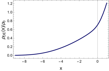
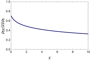
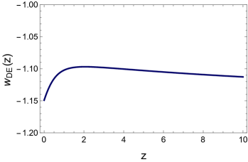
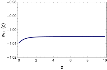
The upper-left panel in Fig. 1 shows as a function of . Observe that RD–MD equilibrium takes place at , while the present epoch corresponds to , since we set . Thus vanishes during RD, and then starts to grow as we enter in the MD epoch. At the present time, , , as determined by the value of , and in the cosmological future () it continues to grow. The upper-right panel shows as a function of redshift , on a scale that emphasizes the recent epoch . The corresponding equation of state (EoS) function is shown in the lower-left panel. Observe that the EoS is phantom, . This is clear from eq. (3.11): since and also its derivative , we must have . With the chosen values of the parameters, we get . Comparing with the commonly used parametrization of the form [91, 92]
| (3.12) |
(where ) in the region , for and we get
| (3.13) |
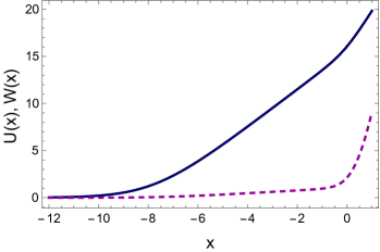
In the lower-right panel of Fig. 1 we plot the evolution of the auxiliary fields. Having set , the field starts from zero and remains zero during RD, as a consequence of the fact that, in RD, the Ricci scalar , so the equation with initial condition gives . However, as we enter in the MD phase, it starts to grow, driving the growth of according to eq. (3.5). In a sense, this behavior is the reflection of a classical instability, related to the fact that is a “ghost-like” field. It is however a welcome instability, since it generates an effective dark energy and self-acceleration. A consequence of this behavior is that and and therefore, as discussed above, a phantom EoS of dark energy, . Indeed, it was realized long ago [93] that a phantom dark energy requires a ghost-like field. Here this behavior is indeed generated by the field which, classically, indeed has a wrong-sign kinetic term [54]. However, as discussed in Section 2.4.4, there are no quanta associated to this field. Thus, in a sense, the field is a “benign” ghost, that classically does the job of inducing an instability that gives a phantom EoS for the dark energy, but does not create consistency problems at the quantum level. We see that the inclusion of nonlocal terms in the quantum effective action naturally produces, in a consistent field-theoretical framework, the “exotic” behavior advocated in [93] as the origin of a phantom dark energy EoS. In this sense, the observation of a phantom dark energy would be a very strong indication in favor of nonlocal models of this class.
It is also interesting to compare the comoving distance in the RR model,
| (3.14) |
to the comoving distance in CDM,
| (3.15) |
as a function of redshift. In Fig. 2 we show the relative difference
| (3.16) |
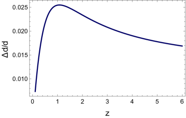
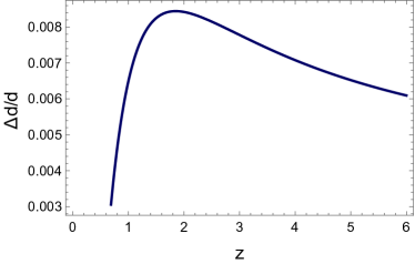
This is of course the same as the relative difference of the luminosity distances , or of the angular diameter distances .151515As we will discuss in Section 3.3.6, this notion of luminosity distance is only appropriate for electromagnetic signals; in the RR model the luminosity distance associated to GW sources is different. We will expand on this in a companion paper [94]. In the left panel we use the same values of and in both eqs. (3.14) and (3.15), to show how the different functional dependence of , with respect to the constant dark energy density of CDM, affects the result. In the right panel we use for each model its own best-fit values obtained by parameter estimation, namely and for RR, and and for CDM (see Table 1). We see that, for the same values of the parameters, at the comoving distance in RR is higher than in CDM by about 2.5 %. However, we also see from the right panel that parameter estimation partially compensates, bringing the relative difference well below . This happens because the model parameters are fitted so to reproduce fixed distance rulers provided by CMB, BAO and SNe.
We next discuss how the results change if we set as initial condition in RD (see also [82, 34]). In principle, a large positive value of during RD could be generated by a previous inflationary era. In any given cosmological era, the function has an approximately constant value , with in dS, in RD and in MD. In the approximation of constant eq. (3.3) can be integrated analytically [29],
| (3.17) |
where the first term on the right-hand side is a solution of the inhomogeneous equations, to which we add the most general solution of the homogeneous equation. Even if, at the beginning of the inflationary era, were small and were at most of order one, at the end of inflation is large because of the linear dependence on of the inhomogeneous term. Setting in eq. (3.17) , as in a de Sitter inflationary phase, we see that in a de Sitter epoch
| (3.18) |
Thus, at the end of inflation , where is the number of inflationary e-folds (recall that ), and the field can enter the RD phase with an initial value . Matching this solution which the RD solution obtained setting in eq. (3.17)
| (3.19) |
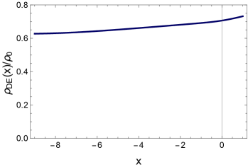
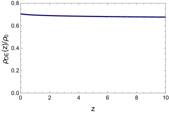
we see that this corresponds to setting at an initial time deep in RD. In contrast, the other auxiliary field enters the RD phase with a negligible value [34]. Fig. 3 shows the results for , corresponding to in a simple inflationary model that ignores reheating [since is constant to great precision during RD, it is irrelevant the exact point in RD when we impose this initial condition]. We see that the DE density is almost constant, and hardly distinguishable from the result in CDM and, for this value of , the DE equation of state differs from by less than , again on the phantom side. Observe also that a different branch of solutions, also potentially viable, at least at the background level, exists if is negative and smaller than a critical value [95].
In the following, when discussing the parameter estimation for the RR model, we will first focus on the case, since this is the case that can be more easily distinguished from CDM with current or near-future observations, but we will also compare with the results for a large value of , chosen to be . The latter is of course more difficult to distinguish from CDM with near-future cosmological observations. However, the RR model with a large value of is also conceptually interesting because it gives an example of a model that generates an effective dark energy that, at least up to the present epoch, behaves almost like a cosmological constant, without however relying on a vacuum energy term, and therefore without suffering from the lack of technical naturalness associated to the cosmological constant.
3.2 Cosmological perturbations
The next step is the study of the cosmological perturbations of the nonlocal model. When performing Bayesian parameter estimation and comparison with CDM we will insert the cosmological perturbation equations in a modified version of the CLASS Boltzmann code. The details on the implementation of the cosmological perturbation equations for the RR model in CLASS have been discussed in detail in appendix A of [32]. In this section we discuss a simpler treatment of the cosmological equations, in which we consider radiation and non-relativistic matter as perfect fluids, neglecting anisotropic stress, neutrino effects, etc. The corresponding equations, which can be quickly integrated numerically, are useful for a first understanding of the behavior of the perturbations. For the RR model the perturbations were studied in great detail in [30] and, for completeness, we will recall the main equations in Section 3.2.2 (see also Section 7.2 of [34] for review). We will also extend the results of ref. [30], studying the dependence of the results on the initial conditions for the perturbations of the auxiliary fields.
We consider here the scalar sector, deferring the discussion of tensor perturbations to Section 3.3.6. We work in the Newtonian gauge, so the metric perturbations in the scalar sector are written as
| (3.20) |
Similarly, we expand perturbatively the auxiliary fields. In the RR model we have two auxiliary fields and , defined in eq. (2.33), or rather and . We then expand the auxiliary fields, writing
| (3.21) |
(in this section we use an overbar to denote background quantities), and we work in terms of the Fourier modes , , , .161616Our conventions on the volume factors in the Fourier transform are the standard ones in the cosmological context, such that, e.g., is dimensionless, see footnote 12 in [30]. In the simplified treatment of this section we use the standard definitions for the perturbations of the energy-momentum tensor of matter (i.e. non-relativistic matter and radiation)
| (3.22) | |||||
| (3.23) | |||||
| (3.24) |
where and are the unperturbed energy density and pressure. Thus, in the energy-momentum tensor the perturbation variables are , , and the anisotropic stress tensor . In the perfect-fluid approximation we take . The pressure perturbations can be written as , where is the speed of sound of the fluid, and we define as usual and ; will refer to radiation, and to matter.
3.2.1 Initial conditions and perturbations of the auxiliary fields
The initial conditions on the metric and matter perturbations are the usual adiabatic initial conditions derived from inflation. For modes that were well outside the horizon at the initial time, when the initial conditions are imposed, they are given by171717Actually, for performing the numerical work, we use the more accurate expressions that also include the corrections of order , where , see eqs. (6.1)–(6.3) of [30].
| (3.25) | |||||
| (3.26) | |||||
| (3.27) |
set at a time deep in RD. We also defined
| (3.28) |
so in particular . The function is related to the amplitude and tilt of the scalar perturbations (at a pivot scale ) by
| (3.29) |
The use, in the nonlocal model, of the standard adiabatic initial conditions derived from inflation is justified by the fact that the energy density associated to the nonlocal term is totally irrelevant during an earlier phase of inflation [34, 82], so the inflationary dynamics in a nonlocal model supplemented by an inflationary sector is exactly the same as in CDM supplemented by the same inflationary sector. This holds because in the RR model there is no instability during an inflationary epoch, neither at the level of background evolution, nor at the level of perturbations [82]. As we mentioned in Section 2.5, this is not the case for the RT model, which is the reason why we do not consider it further.
We must also assign the initial conditions on the perturbations of the auxiliary fields. In refs. [31, 32, 33] the analysis was limited to vanishing initial conditions, i.e.
| (3.30) |
for all Fourier modes (set at some initial time deep in RD). More generally, in Section 3.1 we have seen that, at the background level, i.e. for the homogeneous mode , out of the four quantities , , and , three parametrize irrelevant directions, since the corresponding solutions are quickly attracted toward that obtained with vanishing initial conditions. There is however a marginal direction in parameter space, corresponding to a constant shift , which can also be seen as a shift of the zero mode of the perturbations, . We now wish to understand what is the effect of changing the initial conditions of the modes , , and , with non-vanishing and of the order of the typical comoving momenta relevant for cosmology. We have seen in Sections 2.4.4 and 2.4.5 that the initial conditions of the auxiliary fields are not free parameters corresponding to new degrees of freedom, but rather are in principle fixed in terms of the initial conditions of the metric. In the case of the Polyakov action in , where we have an explicit derivation of the nonlocal quantum effective action from the fundamental theory, we have seen in eq. (2.45) how the initial conditions on the auxiliary fields are related to that of the metric. In particular, if one expands and , eq. (2.45) fixes the initial conditions on the Fourier modes of the perturbation of the auxiliary field, in terms of the initial conditions on the metric perturbation ,
| (3.31) |
For the RR model we do not have a similar derivation of the nonlocal term from a fundamental theory. At first sight, one might fear that our ignorance of the initial conditions on the perturbations of the auxiliary fields will lead to a significant loss of predictivity. However, first of all one must not forget that this effect only enters at first order in cosmological perturbation theory. Furthermore, the explicit example with the Polyakov action allows us to understand that and are driven by the metric perturbations and . In practice, given that anisotropic stresses are negligible and all along the evolution, we can take just as the typical scale for the metric perturbations. From the definition , together with the fact that the perturbations of the Ricci scalar are, parametrically, of order of two derivatives of the metric perturbation , it is natural to assign initial conditions on of the form
| (3.32) |
From the definition together with the fact that, in a cosmological setting, is parametrically of order , it is also natural to take , i.e.
| (3.33) |
We next observe that, for all modes of cosmological relevance, the initial conditions are set at a time when they are well outside the horizon. Thus, the subsequent evolution is the same as that of the mode. In particular, , and parametrize irrelevant directions in parameter space. Any initial value assigned to them is immediately washed out, and the solution quickly reduces to that obtained setting , as we have also checked explicitly by numerical integration.181818Note that, furthermore, for modes well outside the horizon is constant to great accuracy, so , which further renders irrelevant the initial conditions of and . The only direction in parameter space that is marginal, rather than irrelevant, corresponds to . We can then consider initial conditions of the form
| (3.34) |
Actually, the example of the Polyakov action even suggests to take the same value of the constant for all Fourier modes: we see from eq. (3.31) that in this case with for all . In any case, we can also easily check what happens varying independently the constants , for different modes. For some selected modes of cosmological relevance, we will study below how our results depend on , by comparing the case with, e.g., the cases or . As we will see below, the predictions of the RR model turn out to be basically insensitive to variations of in this range (and in fact, even in a much wider range). This is an important result, because it implies that our ignorance on the exact initial conditions for the perturbations of the auxiliary fields does not spoil the predictivity of the model.
3.2.2 Perturbation equations
The perturbation equations for the RR model have been written down in [30], and we recall them here. At the level of perturbations we find convenient to write the equations in terms of
| (3.35) |
instead of . Recall also, from Section 3.1, that the prime denotes the derivative with respect to , while . Perturbing eq. (2.33) one finds
| (3.36) | |||
| (3.37) |
(For readability, we omit here and in the following equations the label from , , etc.) Perturbing eqs. (2.31) and (2.32), using radiation and non-relativistic matter in the energy-momentum tensor, and projecting onto the scalar sector gives
| (3.38) | |||
| (3.39) | |||
| (3.40) | |||
| (3.41) |
which corresponds, respectively, to the perturbations of the component of the modified Einstein equations, the divergence of the component, the trace of the component, and the result of applying the operator to the component. Finally, perturbing the energy-momentum conservation equation we get
| (3.42) | ||||
| (3.43) | ||||
| (3.44) | ||||
| (3.45) |
Of course, because of diffeomorphism invariance, these equations are not all independent. A convenient choice for the numerical integration consists in eliminating from eq. (3.41) and then using (3.36), (3.37), (3.40) and (3.42)–(3.45) as 7 independent equations for the 7 variables . We then use the modified Poisson equation (3.2.2) as a test of the numerical integration, verifying that it is satisfied to high accuracy (one part in to one part in , depending on the value of ) all along the integration. As in [30], we introduce
| (3.46) |
where is the wavenumber of the mode that enters the horizon at matter-radiation equilibrium, and we illustrate our numerical results displaying the results for , and . The mode with re-entered the horizon during RD, the mode with re-entered at matter-radiation equality, and the mode with was outside the horizon during RD and most of MD, and re-entered at . Overall, these three values of illustrate well the dependence of the results, for a large range of scales relevant for cosmology.
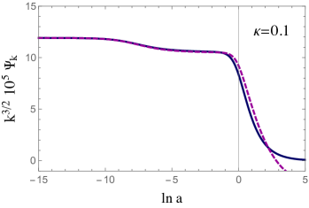
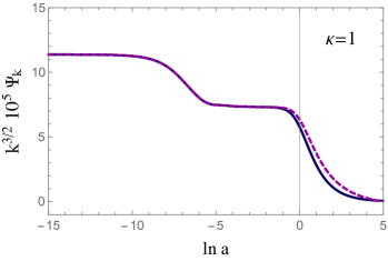
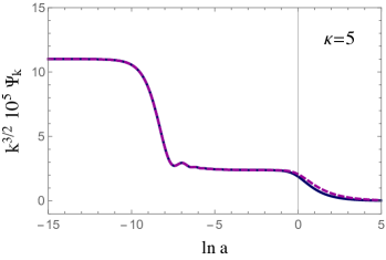
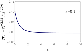
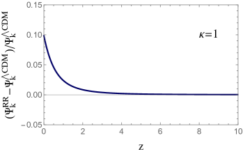

The result of the integration of the perturbation equations is shown in Figs. 4–7. In particular, in Fig. 4 we show the dimensionless quantity against , for our reference values of , in CDM (blue solid line) and in the minimal RR model (i.e. setting ), using for the initial conditions on the perturbations (red dashed line). We see that, up to the present time , the cosmological perturbations of the RR model are very close to that of CDM, and will only start to be significantly different in the cosmological future. Fig. 5 shows the corresponding relative differences as a function of redshift, on a scale that emphasizes the recent cosmological past. We see that the deviations from CDM raise up to about at , with very little dependence on momentum (at least in the cosmological past; from Fig. 4 we see that in the cosmological future the differences, as well as the momentum dependence, can be more significant). This result, already discussed in [30], indicates that the perturbations in the RR model are sufficiently close to that in CDM to be in the right ballpark for fitting the data, yet sufficiently different to be potentially detectable.
We next explore how the results depend on the initial conditions on the cosmological perturbations, i.e. on . Fig. 6 shows, for each of our three reference values of , the evolution of the perturbation with initial conditions (blue solid line), (red dashed line) and , set deep in RD. We see that, by the time that the dark-energy density becomes important, the differences between these solutions have become very small. Fig. 7 shows how this reflects on the evolution of the metric perturbations. Here we show the relative difference between the evolution of in the RR model, comparing the result obtained with a non-vanishing value of and the result for , i.e. we plot
| (3.47) |
For each of our three reference values of , we show the results for (red dashed line) and for (green dot-dashed line). We see that, depending on , the relative differences are of order to . Such relative differences on a quantity, such as , which is already of first order in cosmological perturbation theory, are totally negligible at the present level of accuracy of the analysis (they are rather of the order of terms of second order in perturbation theory). This is a very encouraging result, because it means that our current lack of derivation of the nonlocal model from a fundamental theory, which implies a lack of knowledge of these initial conditions, in practice does not affect the comparison with the data and the predictivity of the model. We will confirm these result in the next section, performing a full Bayesian parameter estimation for the RR model with different initial conditions on the perturbations.
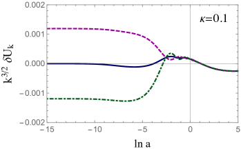
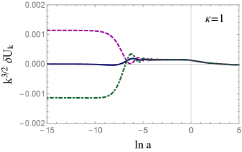
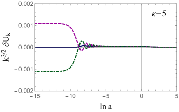
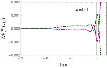
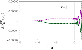
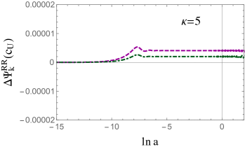
3.3 Bayesian parameter estimation and model comparison
The results of the previous sections show, first of all, that the cosmological perturbations of the RR model are stable [30]. This is already a non-trivial result. For instance the DPG model [96], which opened the way to the study of IR modifications of GR, has a self-accelerated solution [97, 98] but succumbed to fatal instabilities at the level of perturbations [99, 100, 101, 102, 103]. The construction of a consistent theory of massive gravity [104, 105, 106] and of bigravity [107] has provided lasting field-theoretical understanding of the dynamics of massive spin-2 fields. However, once again, their application to cosmology has shown how non-trivial is to build an IR modification of GR with a stable evolution at the background level, as well as at the level of cosmological perturbations; indeed, massive gravity has difficulties already in obtaining a viable background FRW evolution [108]. In bigravity background FRW solutions exist, but, in a branch of solutions that has a dynamical dark energy, the cosmological perturbations are plagued by instabilities in both the scalar and tensor sectors; in a second branch, taking the limit in which the Planck mass associated to the second metric is small, the scalar instabilities can be pushed to unobservably early times, but in this limit the background evolution becomes indistinguishable from that of CDM [109, 110, 111, 112, 113, 114, 115].
Beside being stable, we have seen that, up to the present cosmological epoch, the perturbations in the minimal RR model turn out to be quite close to that of CDM, with differences that (for the minimal model with ) are at most of order 10%; see [30] for several further plots of metric and matter perturbations. This already tells us that this model is in the right ballpark for fitting the cosmological data, yet sufficiently different to be potentially distinguishable from CDM with present and near-future observations. To make more quantitative statements it is necessary to implement these perturbations in a Boltzmann code, perform Bayesian parameter estimation, and see quantitatively how the model fits the data in comparison with CDM. For the RR model this has been done in [30, 31, 32, 33], and here we will expand on these results. We have implemented the cosmological equations in CLASS [116], and constrained the nonlocal model with observations using the Markov Chain Monte Carlo (MCMC) code Montepython [117]. The details on the implementation of the RR model in CLASS have been discussed in appendix A of [32].
It should also be appreciated that we are considering a model in which we simply have a new parameter, , that replaces the cosmological constant in CDM, and which has a well-defined physical meaning, as a dynamically-generated mass term for the conformal mode; see eq. (2.23) [plus a hidden parameter, that, as we have seen, enters in the initial conditions of the auxiliary field , and whose value could be related to the duration of a primordial inflationary phase; see the discussion below eq. (3.18)]. In contrast, modified gravity models that have been intensely studied in the literature in recent years involve either a free function of , as in theories [118], or a free function of , as in the Deser-Woodard model [20], or even a set of arbitrary functions of a (hypothetical) scalar or massive vector field, as for instance in Horndesky [119, 120] and beyond-Horndeski theories [121], or in generalized Proca theories [122]. There is no theoretical clue on the form of these functions, leading to highly redundant (and, sometimes, quite baroque) alternatives to CDM. Furthermore, it should be observed that these modified gravity models have usually been compared to CDM using, rather than the full available CMB information, only the “shift parameter” (see e.g. [123]), which is just an approximate indicator of the position of the first peak. However, it is not difficult to adjust a model to this single data point, especially if one can play with extra free parameters (and even free functions). The test to which we are submitting our nonlocal model, involving the full information on the CMB multipoles of temperature (and also of polarization) is much more stringent. Furthermore, the minimal RR model with has the same number of parameter as CDM. Here we will just consider two cases, and equal to a large value, that we will choose as , and we will not vary as a free parameter. Even if one would optimize the results with respect to , this would just give a model with one parameter more than CDM, which is still much more economical than models in which one can play with free functions.
3.3.1 Datasets
-
•
CMB. We use the 2015 Planck [124] measurements of the angular (cross-)power spectra of the CMB. In particular, we take the full-mission lowTEB data for low multipoles () and the high- Plik TT,TE,EE (cross-half-mission) ones for the high multipoles () of the temperature and polarization auto- and cross- power spectra [125]. We also include the temperaturepolarization (TP) lensing data, using only the conservative multipole range [126, 127].
-
•
Type Ia supernovae. We use the JLA data for SN Ia provided by the SDSS-II/SNLS3 Joint Light-curve Analysis [128].
- •
Initially we will compare the models to CMB+BAO+SNa data, without including a prior on , since it is interesting to see how the prediction of the RR model obtained just from CMB+BAO+SNa compares with the local measurement. We will see that the tension that exists in CDM is significantly reduced in the RR model. We will then add to our datasets also the value of obtained from local measurements, using [132]
| (3.48) |
in the usual units of .
3.3.2 Free parameters
The Planck baseline analysis for CDM uses six independent cosmological parameters: the Hubble parameter today , the physical baryon and cold dark matter density fractions today and , respectively, the amplitude and tilt of the primordial scalar perturbations [defined in eq. (3.29)], and the reionization optical depth . Note that, assuming flatness, is a derived parameter, fixed by the flatness condition. In the nonlocal models we have a mass scale which replaces the cosmological constant, and again can be taken as a derived parameter, fixed by the flatness condition. Thus, for the RR model, we can take the same six independent cosmological parameters, as in CDM.
An important point is, however, the treatment of the sum of neutrino masses, . Oscillation experiments provide a lower bound eV [133], assuming a normal mass hierarchy dominated by the heaviest neutrino mass eigenstate. The Planck baseline analysis sets to a fixed value corresponding to the lower limit, eV. As discussed in the Planck paper [83], there is actually no compelling theoretical reason for this choice, and there are other possibilities, including a degenerate hierarchy with eV.
If one rather leaves as a free parameter when analyzing the cosmological data, in CDM one finds that the one-dimensional marginalized likelihood for has its maximum at (see Fig. 30 of [83]), and this marginalized likelihood implies an upper bound eV (at 95% c.l.) (combining Planck TT+lowP+lensing+) [83]. In other words, if one performs the analysis in CDM letting free the neutrino masses with a prior eV, as required by oscillation experiments, the Planck data drive the value of back to the lower limit eV.
As observed in [33], the situation is different in the RR nonlocal model. In that case, letting the neutrino masses as free parameters, one finds a one-dimensional marginalized likelihood for that is peaked at a nonzero value, which is between the lower limit set by oscillation experiments and the upper limit from -decay experiments.191919Tritium -decay experiments give an upper limit eV, which can be translated into eV assuming three species of degenerate neutrinos (in any case, the precise value of the upper limit will be of no relevance in the following, since the value of predicted by the nonlocal models is anyhow well below these upper limits). This fact has two important implications:
-
1.
The (minimal) RR model provides a prediction for the value of the sum of the neutrino masses. In contrast, in CDM for the best-fit value one simply gets back the value of the prior that one has put in, and one can only obtain an upper limit on .
-
2.
When comparing the performances of the RR model to that of CDM, it is essential to let the neutrino masses as free parameters. Indeed, in [32], performing Bayesian parameter estimation and fitting to CMB+BAO+SNa data, it was found that the RR model appeared to be disfavored with respect to CDM, with moderate-to-strong evidence. We now understand this as an artifact due to the fact that, in [32], the Planck baseline analysis was applied also to the nonlocal models, fixing eV. However, this amounts to arbitrarily fixing a parameter, which a priori is free, or at least constrained by oscillation and -decay experiments within some range, to the value preferred by CDM. Obviously, this has the effect of favoring CDM over RR. Once the sum of neutrino masses is included among the free parameters, both in the RR model and in CDM, the situation changes. In CDM it will go toward zero or, if we impose a prior eV, it will hit the prior. In contrast, in the RR model it goes to its own best-fit value, which is different. Then, from the corresponding chi-squares or Bayes’ factors, one finds that the RR and CDM model are statistically equivalent from the point of view of fitting the data [33].
Thus, in the following, we will perform Bayesian parameter estimation for CDM and the RR model, and we will compare their performances using, as free parameters, the set
| (3.49) |
For CDM we will actually examine two cases, corresponding to fixing eV, which allows us to make contact with the Planck baseline analysis (column labeled CDM in the following tables) and letting it as a free parameter (column labeled CDM), which will allow us to make a more homogeneous comparison with the RR model, in which neutrino masses are always taken as free parameters. For the RR model, in contrast, we only give the results for the case in which the sum of neutrino masses is allowed to vary freely, since fixing it to eV for this model as little meaning. For the RR model, we show the results for the “minimal model” with , as well as for a model with a large value, , as suggested by the evolution during a previous inflationary phase.
3.3.3 Results using Planck+BAO+JLA
In Table 1 we show the Bayesian parameter estimation and the resulting for CDM, CDM and the RR model, using the dataset combination Planck+BAO+JLA. In this table, for the RR model the initial condition of the perturbation is set to zero. We will show later that varying the parameter in eq. (3.34) has basically no effect. Beside the values of the seven fundamental independent parameters (3.49), we also give some useful derived parameters, namely and the reionization redshift , and we show the corresponding as well as the differences in , taken here with respect to the value for CDM. Two main conclusions can be drawn from these results.
| CMB+BAO+SNe | ||||
| Parameter | CDM | CDM | RR | RR |
| (at ) | (at ) | |||
| 100 | ||||
| 13631.04 | 13630.78 | 13634.40 | 13630.68 | |
| 0.26 | 0 | 3.62 | -0.10 | |
-
1.
Using Planck+BAO+SNe data, the minimal RR model predicts
(3.50) in the usual units . Compared to the value from local measurements [132], the difference is now only , which hardly qualifies as a tension. In contrast, in CDM and in CDM we find a discrepancy.202020When deriving the value of a parameter and its error through a MCMC, there is unavoidably a fluctuation in the central value due to the stochastic nature of a MCMC. The central value for that we get from our MCMC for CDM is however in excellent agreement with the value found by Planck marginalizing over neutrino masses and using Planck+BAO+JLA+, see eq. (58) of [83]. Note that here we have not yet used in our dataset.
-
2.
The Planck+BAO+JLA dataset, interpreted within CDM, provides no evidence for non-vanishing neutrino masses, and only gives an upper limit eV.212121This bound is slightly stronger than the bound eV given in eq. (54d) of [83], where only Planck+BAO data were used. In contrast the same dataset, interpreted within the minimal RR model, provides clear evidence for non-vanishing neutrino masses, and the prediction
(3.51) that nicely falls within the window provided by oscillation and beta-decay experiments.
The predictions for and are the two most significant phenomenological results of the minimal RR model. Fig. 8 shows the two-dimensional marginalized likelihood in the plane for the minimal RR model, compared to the prediction of CDM, to the lower limit on neutrino masses, and to the value of from local measurements. We see that the predictions of the RR model are more consistent both with the lower limit on the sum of neutrino masses, and with the local measurement.
From Table 1 we also see that the RR model with a large value of becomes very close to CDM, a result that was expected already from the background evolution shown in Fig. 3.
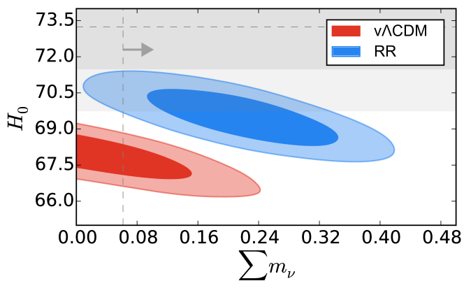
The differences in the are reported in the last line of Table 1. We recall that, for models with the same number of free parameters, as CDM and the minimal RR model, the conventional interpretation is that a difference implies statistical equivalence between the two models, while suggests “weak evidence” in favor of the model with lower , and indicates “strong evidence” in favor of the model with lower . The value in Table 1 indicates weak evidence in favor of CDM.
Finally, we study the effect of varying the constant that determines the initial conditions on , see eq. (3.34). As discussed there, the natural size for the initial conditions on is fixed by the metric perturbation , so we expect . For instance, for the Polyakov action we found that ; see eq. (3.31). Here, for definiteness, we have run some further MCMC setting or . The results are shown in Table 2, and confirm that variation of the initial conditions of this order have a negligible effect on the results.
| CMB+BAO+SNe | |||
| Parameter | RR | RR | RR |
| 100 | |||
| 13634.34 | 13634.40 | 13634.28 | |
| 0.06 | 0.12 | 0 | |
3.3.4 Results using Planck+BAO+JLA+
Until now, when performing Bayesian parameter estimation, we have not included the local measurements, since an important question that we wanted to answer was whether, in the nonlocal model, the prediction for obtained from the Planck+BAO+JLA dataset gives a result consistent with that of the local measurements. When one looks at the data through the “glasses” of CDM there is a natural tendency not to mix the local measurement with the Planck+BAO+JLA dataset, since they are in tension, and one rather appeals to the possible existence of some unaccounted systematic effect. However, when comparing the performances of two models, it is correct to insert also this data point in the analysis. Discarding it a priori, assuming that it might be due to some hitherto unexplained systematics, would be a form of bias in favor of CDM. If we want to test CDM against other models, we cannot perform a “cherry picking” of the observations, excluding those that produce tensions in CDM, unless clear evidence for systematic errors is unveiled. We have therefore performed further runs of the MCMC, adding also the value (3.48) to the Planck+BAO+JLA dataset. The results are shown in Table 3. The value of in the minimal RR model now further raises to . We also see that now the best chi-square is provided by the minimal RR model, although the difference is not statistically significant.
| CMB+BAO+SNe+() | ||
| Parameter | CDM | RR |
| (at ) | ||
| 100 | ||
| 13639.26 | 13638.26 | |
| 0 | -1.0 | |
The prediction for the sum of the neutrino masses now becomes
| (3.52) |
3.3.5 Structure formation
We next explore how well the minimal RR model and CDM fit structure formation data. In Fig. 9 we plot a compilation of measurements of at different redshifts and we compare with the predictions of the minimal RR model and of CDM, using for the theoretical prediction the mean values and errors obtained from CMB+BAO+SNe+ given in Table 3. We find that the is lower in CDM, compared to the minimal RR model, with a difference . Adding this to the value found from the comparison with Planck+BAO+JLA+ data (see again Table 3) we find that, overall, CDM is favored, with respect to the minimal RR model, with a , corresponding to statistical equivalence between the two models. We have also repeated the analysis using the mean values and errors obtained from CMB+BAO+SNe, without , given in Table 1. In this case again the from structure formation is lower in CDM, with , which, together with the value in Table 1, gives corresponding to weak evidence in favor of CDM.
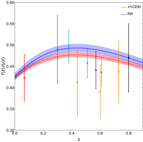
3.3.6 Speed and propagation of gravitational waves
The recent observation by the LIGO and Virgo interferometers of the GWs from the neutron star binary coalescence GW170817 [140] and of the associated -ray burst GRB 170817A by Fermi-GBM [141] and INTEGRAL [142] provides a test of the speed of gravitational waves (GWs), at the level [143] (where the exact lower limit on depends on the assumptions on the delay between the GW and GRB emission times). This puts a further significant constraint on modified gravity theories. For instance, this observation rules out a large class of Horndesky theories, leaving only those that are conformally coupled to gravity, i.e. of the form [144, 145, 146, 147]. Let us therefore see how nonlocal gravity performs from this point of view.
We recall, first of all, that in GR tensor perturbations over a FRW background satisfy
| (3.53) |
where are the Fourier modes of the GW amplitude, labels the two polarizations, denotes conformal time, , and the source term is related to the anisotropic stress tensor. For the propagation in empty space we can set . It is convenient to introduce a field from
| (3.54) |
Then eq. (3.53) becomes
| (3.55) |
On dimensional grounds, . For sub-horizon modes , and therefore can be neglected compared to . Observe that, for the GWs detected by LIGO/Virgo, the typical frequency around merger is Hz, corresponding to a reduced wavelength km. This is ridiculously small compared to the present Hubble scale , to the extent that . Therefore the term in eq. (3.55) is totally negligible with respect to even when we study deviations in the speed of GWs at the level , and we can write simply
| (3.56) |
This shows that the dispersion relation of tensor perturbations is , i.e. GWs propagate at the speed of light (that we have set to one). On the other hand, the factor in eq. (3.54) combines with the factor (where is the comoving distance) obtained when computing GW emission in the local wave zone (i.e., sufficiently far from the source that the behavior of the GW sets in, but still sufficiently close that the cosmological expansion can be neglected) to produce an overall behavior over cosmological distances
| (3.57) |
One then defines the luminosity distance from
| (3.58) |
where the factor is inserted to reabsorb the factors that appear when passing from the radiated energy and time in the source frame to the corresponding quantities in the detector frame (see e.g. eq. (4.158) of [148]). Then
| (3.59) |
In the waveform produced by the inspiral of a compact binary the factor is then absorbed into a redefinition of the chirp mass (together with analogous factors coming from the passage from the source-frame frequency and the detector-frame frequency of the signal; see Section 4.1.4 of [148]), and the waveform is finally proportional to .
Let us now perform the same analysis for GWs in the RR model. The equation governing the evolution of tensor perturbations over FRW in the RR model has been derived in [32], and reads
| (3.60) |
where is the background evolution of the auxiliary field defined in eq. (3.35). Thus, for the free propagation we have
| (3.61) |
where
| (3.62) |
and, as usual, (where , and we used .222222Similar modified propagation equations have been found in other modified gravity models: in particular, in the DGP model [96], at cosmological scales gravity leaks into extra dimensions, affecting the propagation equation of tensor modes [149]. Modified GW propagation can be included in the general framework of the effective field theory approach to dark energy [150, 151, 152], and has also been found in some scalar-tensor theories of the Horndeski class [153, 154, 155]. We now introduce from
| (3.63) |
where
| (3.64) |
and we get
| (3.65) |
Once again, inside the horizon we can neglect , and we see that GWs propagate at the speed of light also in the RR model. The RR model therefore passes the test from GW170817/GRB 170817A.
However, we see that there is an interesting difference in the propagation of GWs in the RR model, with respect to GR, due to the fact that the GW amplitude now scales as rather than . This means that, rather than being just proportional to , the GW amplitude observed today, after the propagation from the source to the observer, will have decreased by a factor instead of a factor , where the label refers to the emission time (at redshift ) and the observation time, at redshift zero. Therefore
| (3.66) |
where is the usual notion of luminosity distance appropriate for electromagnetic signals and, since only the ratios and enter, without loss of generality we can choose the normalizations .
Thus, we see that in the RR model there are two different notions of luminosity distance (or of comoving distance). One appropriate for electromagnetic signals, which is given by the usual expression
| (3.67) |
corresponding to the comoving distance given in eq. (3.14), and a GW luminosity distance
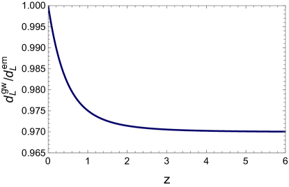
| (3.68) |
appropriate for the propagation of GWs. The factor is obtained by integrating eq. (3.64), which gives
| (3.69) |
The background evolution is obtained from the results presented in Section 3.1 and the corresponding result for the ratio in the RR model is shown in Fig. 10. We see that, at , the two notions of luminosity distance differ by about . This means that, in the RR model, “standard sirens” would not measure the same luminosity distance as standard candles, and this correction will have to be taken into account when using standard sirens to infer the cosmological parameters in the RR model. In a companion paper [94] we will elaborate on this point and discuss the possibility of using standard sirens to distinguish CDM from the (minimal) RR model with third-generation GW interferometers such as the Einstein Telescope.
One can similarly show, using eq. (27) of [32], that also in the RT model GWs propagate at the speed of light, but the GW luminosity distance is different from the electromagnetic luminosity distance. The same holds if, in the RR or RT models, we replace with . For the non-local model (2.52), we will show in Appendix A that the situation is different, and GWs do not propagate at the speed of light, and in fact this rules out the model.
4 Conclusions
The basic physical assumption of our approach is that, because of infrared quantum fluctuations, gravity develops a mass scale, which modifies its IR behavior. We have explored different possible implementations of this idea, and we have found that the model that turns out to work well corresponds to giving a mass to the conformal mode; see eq. (2.23). Naively, one would think that the only way to give a mass to some component of the metric is to break the invariance under diffeomorphisms. This is the route taken in massive gravity or in bigravity, where the spin-2 mode becomes massive because of the addition of terms that break the original diff invariance. However, this is true only if we want to include a mass term at the level of the fundamental action. If a mass is generated dynamically by quantum effects, it will not appear in the fundamental action, but rather in the quantum effective action. The latter, as we have reviewed in Sections 2.1 and 2.2, always include nonlocal terms whenever the fundamental theory has massless particles, such as the graviton. With nonlocal terms it is possible to construct diffeomorphism-invariant quantities that, expanded to second order in the field, correspond to a mass term. A completely similar situation takes place for gauge fields. Naively, one would think that the only way to give a mass to a gauge field is to break gauge invariance, and this is what is done, for instance, to give masses to the and bosons. However, this is not the only possibility and, indeed, in QCD the gluons are believe to get an effective mass through the nonlocal term (2.20) in the quantum effective action, generated non-perturbatively by the strong IR effects of QCD. Similarly, we have postulated that in GR the conformal mode gets an effective mass through the addition of a nonlocal term to the gravity quantum effective action, of the form given in eq. (1.1).232323The fact that it is just the conformal mode that gets a dynamical mass matches well the result in [14], that show that, in de Sitter space, the strongest IR divergences come from the long-distance behavior of the propagator of the conformal mode. In this sense, strictly speaking, we believe that our proposal does not even belong to the class of “modified gravity” theories. We are not modifying Einstein-Hilbert gravity as a fundamental theory, but we are rather trying to capture its leading quantum effects in the infrared.
Nonlocal terms might sound unfamiliar, particularly to most cosmologists, that are used to work with classical actions. However, it is a fact that they appear in the quantum effective action. Once properly understood, their use does not create any special conceptual nor technical difficulty, as we have discussed in detail in Section 2.4. At most, one might have to face the problem of choosing the boundary condition for the nonlocal operator, or equivalently for the auxiliary fields introduced for writing the theory in a local form. In the RR model, we have seen that this just amounts to having to deal with one extra free parameter, . Indeed, once one overcomes the “psychological barrier” of thinking in terms of quantum effective actions, and therefore allowing for nonlocal terms, one realizes that a model such as the RR model is much more elegant, simple and attractive than the typical modified gravity models that proliferated in the recent literature. It has only one new parameter, the mass scale , that has a physically clear and well-defined meaning as a mass term for the conformal mode, and that replaces the cosmological constant in CDM (plus a hidden parameter related to the initial conditions of the nonlocal operator). In contrast, modified gravity models that have been recently much studied in the literature typically involve several arbitrary functions of new hypothetical fields, with no physical clue on the form of these functions, and often a level of complication that eventually makes them look somewhat baroque, even more considering that they are meant to be an alternative to a simple cosmological constant.
At the phenomenological level, we have seen that the RR model works very well. If we compare its performances to that of CDM by using CMB, BAO, SNe, local measurements of and structure formation data, the two models fits the data at a statistically equivalent level. However, the RR model (in its minimal form, with ) has two particularly interesting predictions: a higher value of , which reduces the tension with local measurement (bringing it down to the level if we estimate from CMB+BAO+SNe only), and a value for the neutrino masses which agrees well with the limit from oscillation experiments. In contrast, in CDM, where we let the neutrino masses as free fitting parameters, the one-dimensional likelihood for the sum of the neutrino masses is peaked in zero. These results are shown in Fig. 8, which displays the two most interesting predictions of the RR model, and compares them to the predictions of CDM. Observe, from Fig. 8, that a direct measurement of the neutrino masses from particle physics experiments could provide decisive evidence for the RR model, compared to CDM. Near-future cosmological observations should also be able to discriminate between the RR model and CDM, or at least put stringent bounds on the parameter which basically interpolates between the two. In separate publications will be discussed the forecasts for the RR model for future surveys such EUCLID, SKA and DESI [156] and for a third-generation GW detector such as the Einstein Telescope [94].
Acknowledgments. We thank Giulia Cusin for very useful discussions. The work of the authors is supported by the Fonds National Suisse and by the SwissMap National Center for Competence in Research.
Appendix A The model
The non-local model (2.52) was introduced in [68], where it was only studied at the background level. There it was found that its DE equation of state is significantly different from , with a value . Comparison with the Planck limits on [125] then already suggested that the model will not fit well the data, although, as was mentioned, a full analysis of the perturbations is necessary to reach a definite conclusion. Here we perform such an analysis. We will see that, in fact, the model is already ruled out by the behavior of tensor perturbations, that do not propagate with the speed of light. However, the study of the scalar sector of this model is also methodologically interesting. In fact, in general, in modified gravity models, a DE equation of state on the phantom side has the effect of rising the value of obtained from parameter estimation, and indeed the value of obtained from local measurements could be obtained in a wCDM model with [157]. So, the study of the scalar sector of the model is interesting because its DE equation of state is expected to be about the most phantom that one can have in order to fit reasonably the CMB+BAO+SNe data, and then its prediction for will give an idea of the maximum value of that could be obtained from models of this type.
It is also conceptually interesting to observe that the model (2.52) interpolates between the RR model and a model with a non-trivial form factor for Newton’s constant. This can be seen more easily in de Sitter space, where is constant and , so eq. (2.53) simplifies to
| (A.1) |
Then, after integrations by parts, the effective action (2.52) becomes
| (A.2) |
For Fourier modes such that , this reduces to the RR model. In the opposite limit , in contrast
| (A.3) |
corresponding to a running Newton’s constant. We next recall the main results on the background evolution of the model, and we work out its cosmological perturbations.
Background evolution. The covariant equation of motion derived from (2.52) are242424We have corrected a typo in eq. (4.4) of [68]. This typo did not affect any other equation or result in that paper.
| (A.4) |
where is defined by
| (A.5) |
Specializing to FRW, the background evolution equations are [68]
| (A.6) |
where again , while now
| (A.7) |
and, following [68], we have introduced two auxiliary fields
| (A.8) | |||||
| (A.9) |
where is conformal time (recall that, in contrast, the prime denotes , where ). The introduction of the two fields allows us to split the fourth-order equation into a couple of second-order equations,
| (A.10) | |||||
| (A.11) |
Setting constant we find that the most general solution of eq. (A.10) is
| (A.12) |
Therefore both homogeneous solutions are decaying modes, in all cosmological epochs, and even the inhomogeneous solution is constant, rather than linearly growing in as in eq. (3.17). The same holds for , since the homogeneous equation has the solutions with and . Again, is negative in all three eras, while is negative in RD and MD and vanishes, corresponding to a constant solution, in dS. Thus, there is no growing mode and the cosmological evolution is stable. Thus, even if we set the initial conditions of order one for and in a earlier inflationary epoch, and still enter the RD era with a value of order one. In RD , so the inhomogeneous term in eq. (A.12) vanishes, and for the de Sitter solution is matched to the two decaying modes and . Thus, the solution is quickly attracted toward the one obtained setting deep in RD. Similarly, for the solution that emerges from de Sitter is matched to its two decaying modes in RD. Thus, the solution obtained setting the initial conditions at some initial time deep in RD is an attractor and, in the model there is no free parameter associated to the boundary conditions (contrary to the RR model, where we have ). This makes the model very predictive.252525In fact, even if one set large initial values for and at the beginning of RD, the exponential decay during RD brings them back, to high accuracy, to the solution obtained with vanishing initial conditions.
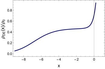
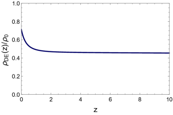
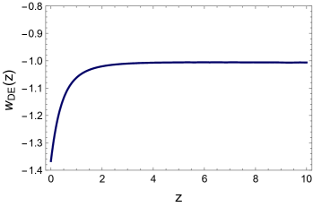
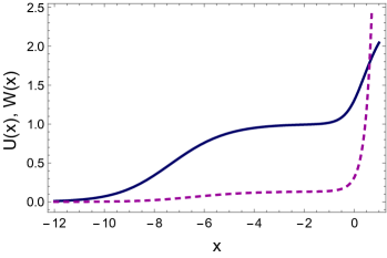
We can now integrate numerically the equations of motion, with initial conditions at some initial time deep in RD. The result of the numerical integration is shown in Fig. 11 [68]. As in the RR model, we have an effective dark energy density . We see that, once again, the effective DE density vanishes deep in RD, and begins to grow as we approach radiation-matter equality (around ). In the model, during MD eventually stabilizes to a constant, leading to a long phase where the EoS parameter as in CDM. However, as the DE density starts to dominate over matter, finally grows again, leading near to an EoS which is substantially more phantom than in the RR model, with (with the choice and obtained from parameter estimation in this model, see below). Using again the parametrization (3.12) in the region , for our best-fit values and we get and .
Cosmological perturbations in the scalar sector. At the perturbation level we write the metric in the scalar sector as in eq. (3.20). The auxiliary field defined in eq. (A.5) satisfies the fourth-order equation . To keep the equations as close as possible to that of the RR model, we find convenient to split this fourth-order equation into a pair of second-order equation, introducing a second auxiliary field. In a generic space-time, it is not possible to perform this split covariantly [although this would be possible in de Sitter, see eq. (A.1)], so we simply keep the definitions (A.8, A.9) also when performing perturbations over an FRW background, i.e. we write and . Similarly to the RR model, for studying the perturbations it is convenient to use the variable rather than . We then expand . As a second perturbation variable for the auxiliary field, instead of , it is convenient to chose
| (A.13) |
because then higher-derivative terms drop out of the equations. The above equation can be taken as a dynamical equation for , while for one finds
| (A.14) | |||
The analogous of eqs. (3.2.2)–(3.41) are
| (A.15) | |||
| (A.16) | |||
| (A.17) | |||
| (A.18) |
Finally, eqs. (3.42)–(3.45) are of course unchanged, since they express the linearization of the energy-momentum tensor, and are therefore model-independent. The results of the numerical integration shows that the cosmological perturbations are again stable and relatively close to those of CDM.
| CMB+BAO+SNe | ||
| Parameter | CDM | |
| (at ) | ||
| 100 | ||
| 13630.78 | 13649.98 | |
| 0 | 19.20 | |
| CMB+BAO+SNe+ | ||
| Parameter | CDM | |
| (at ) | ||
| 100 | ||
| 13639.26 | 13651.86 | |
| 0 | 12.6 | |
Parameter estimation for the model. We have then implemented the perturbations in our Boltzmann code and performed Bayesian parameter estimation. The results are shown in Table 4 (using CMB+BAO+SNe) and Table 5 (using CMB+BAO+SNe +). For easy of comparison, we write again the results for CDM already shown in Tables 1 and 3, and we give the difference in compared to CDM. We see that the model indeed predicts a higher value of , although not sensibly higher than that in the RR model. On the other hand, its is significantly worse than than that of CDM, even including in the dataset, so the model is already very strongly disfavored by the study of the scalar perturbations.
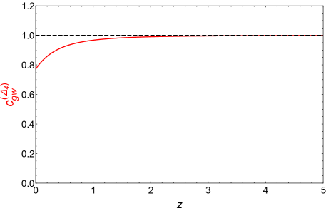
Tensor perturbations. On top of this, we find that the model is ruled out by the fact that its tensor perturbations do not propagate at the speed of light. This is also interesting from the methodological point of view since it shows that, for these nonlocal models, it is not obvious a priori to satisfy this constraint. The equation for tensor perturbations in the model is
| (A.19) |
and the corresponding speed of gravitational waves in a FRW background is
| (A.20) |
This quantity is always smaller than one, and in the recent epoch it differs from one significantly, see Fig. 12. Thus, the model is ruled out by the GW170817/GRB 170817A test.
References
- [1] N. Birrell and P. Davies, Quantum fields in curved space. Cambridge University Press, 1982.
- [2] A. Barvinsky and G. Vilkovisky, “The Generalized Schwinger-DeWitt Technique in Gauge Theories and Quantum Gravity,” Phys.Rept. 119 (1985) 1.
- [3] A. Barvinsky and G. Vilkovisky, “Beyond the Schwinger-DeWitt Technique: Converting Loops Into Trees and In-In Currents,” Nucl.Phys. B282 (1987) 163.
- [4] I. L. Buchbinder, S. D. Odintsov, and I. L. Shapiro, Effective action in quantum gravity. Institute of Physics, Bristol, UK, 1992.
- [5] V. Mukhanov and S. Winitzki, Introduction to quantum effects in gravity. Cambridge University Press, Cambridge, 2007.
- [6] I. L. Shapiro, “Effective Action of Vacuum: Semiclassical Approach,” Class. Quant. Grav. 25 (2008) 103001, 0801.0216.
- [7] A. A. Starobinsky and J. Yokoyama, “Equilibrium state of a selfinteracting scalar field in the De Sitter background,” Phys. Rev. D50 (1994) 6357–6368, astro-ph/9407016.
- [8] A. Riotto and M. S. Sloth, “On Resumming Inflationary Perturbations beyond One-loop,” JCAP 0804 (2008) 030, 0801.1845.
- [9] C. Burgess, L. Leblond, R. Holman, and S. Shandera, “Super-Hubble de Sitter Fluctuations and the Dynamical RG,” JCAP 1003 (2010) 033, 0912.1608.
- [10] A. Rajaraman, “On the proper treatment of massless fields in Euclidean de Sitter space,” Phys. Rev. D82 (2010) 123522, 1008.1271.
- [11] M. Beneke and P. Moch, “On dynamical mass generation in Euclidean de Sitter space,” Phys. Rev. D87 (2013) 064018, 1212.3058.
- [12] F. Gautier and J. Serreau, “Infrared dynamics in de Sitter space from Schwinger-Dyson equations,” Phys. Lett. B727 (2013) 541–547, 1305.5705.
- [13] D. López Nacir, F. D. Mazzitelli, and L. G. Trombetta, “ model in Euclidean de Sitter space: beyond the leading infrared approximation,” JHEP 09 (2016) 117, 1606.03481.
- [14] I. Antoniadis and E. Mottola, “Graviton Fluctuations in De Sitter Space,” J.Math.Phys. 32 (1991) 1037–1044.
- [15] I. Antoniadis and E. Mottola, “4-D quantum gravity in the conformal sector,” Phys.Rev. D45 (1992) 2013–2025.
- [16] N. C. Tsamis and R. P. Woodard, “Strong infrared effects in quantum gravity,” Annals Phys. 238 (1995) 1–82.
- [17] S. P. Miao, N. C. Tsamis, and R. P. Woodard, “Gauging away Physics,” Class. Quant. Grav. 28 (2011) 245013, 1107.4733.
- [18] A. Rajaraman, “de Sitter Space is Unstable in Quantum Gravity,” Phys. Rev. D94 (2016), no. 12 125025, 1608.07237.
- [19] C. Wetterich, “Effective nonlocal Euclidean gravity,” Gen.Rel.Grav. 30 (1998) 159–172, gr-qc/9704052.
- [20] S. Deser and R. Woodard, “Nonlocal Cosmology,” Phys.Rev.Lett. 99 (2007) 111301, 0706.2151.
- [21] R. Woodard, “Nonlocal Models of Cosmic Acceleration,” Found.Phys. 44 (2014) 213–233, 1401.0254.
- [22] S. Park and S. Dodelson, “Structure formation in a nonlocally modified gravity model,” Phys.Rev. D87 (2013) 024003, 1209.0836.
- [23] H. Nersisyan, A. F. Cid, and L. Amendola, “Structure formation in the Deser-Woodard nonlocal gravity model: a reappraisal,” JCAP 1704 (2017) 046, 1701.00434.
- [24] S. Park, “Revival of the Deser-Woodard nonlocal gravity model: Comparison of the original nonlocal form and a localized formulation,” 1711.08759.
- [25] A. Barvinsky, “Nonlocal action for long distance modifications of gravity theory,” Phys.Lett. B572 (2003) 109, hep-th/0304229.
- [26] A. Barvinsky, “Dark energy and dark matter from nonlocal ghost-free gravity theory,” Phys.Lett. B710 (2012) 12–16, 1107.1463.
- [27] A. O. Barvinsky, “Serendipitous discoveries in nonlocal gravity theory,” Phys.Rev. D85 (2012) 104018, 1112.4340.
- [28] M. Maggiore and M. Mancarella, “Non-local gravity and dark energy,” Phys.Rev. D90 (2014) 023005, 1402.0448.
- [29] M. Maggiore, “Phantom dark energy from nonlocal infrared modifications of general relativity,” Phys.Rev. D89 (2014) 043008, 1307.3898.
- [30] Y. Dirian, S. Foffa, N. Khosravi, M. Kunz, and M. Maggiore, “Cosmological perturbations and structure formation in nonlocal infrared modifications of general relativity,” JCAP 1406 (2014) 033, 1403.6068.
- [31] Y. Dirian, S. Foffa, M. Kunz, M. Maggiore, and V. Pettorino, “Non-local gravity and comparison with observational datasets,” JCAP 1504 (2015) 044, 1411.7692.
- [32] Y. Dirian, S. Foffa, M. Kunz, M. Maggiore, and V. Pettorino, “Non-local gravity and comparison with observational datasets. II. Updated results and Bayesian model comparison with CDM,” JCAP 1605 (2016) 068, 1602.03558.
- [33] Y. Dirian, “Changing the Bayesian prior: Absolute neutrino mass constraints in nonlocal gravity,” Phys. Rev. D96 (2017) 083513, 1704.04075.
- [34] M. Maggiore, “Nonlocal Infrared Modifications of Gravity. A Review,” Fundam. Theor. Phys. 187 (2017) 221–281, 1606.08784.
- [35] C. W. Misner, K. Thorne, and J. Wheeler, Gravitation. Freeman, New York, 1973.
- [36] R. Jordan, “Effective Field Equations for Expectation Values,” Phys.Rev. D33 (1986) 444.
- [37] E. Calzetta and B. Hu, “Closed Time Path Functional Formalism in Curved Space-Time: Application to Cosmological Back Reaction Problems,” Phys.Rev. D35 (1987) 495.
- [38] D. A. Dalvit and F. D. Mazzitelli, “Running coupling constants, Newtonian potential and nonlocalities in the effective action,” Phys.Rev. D50 (1994) 1001–1009, gr-qc/9402003.
- [39] A. V. Manohar, “Effective field theories,” Lect.Notes Phys. 479 (1997) 311–362, hep-ph/9606222.
- [40] A. Dobado and A. L. Maroto, “Particle production from nonlocal gravitational effective action,” Phys.Rev. D60 (1999) 104045, gr-qc/9803076.
- [41] Yu. V. Gusev and A. I. Zelnikov, “Finite temperature nonlocal effective action for quantum fields in curved space,” Phys. Rev. D59 (1999) 024002, hep-th/9807038.
- [42] E. V. Gorbar and I. L. Shapiro, “Renormalization group and decoupling in curved space,” JHEP 0302 (2003) 021, hep-ph/0210388.
- [43] E. V. Gorbar and I. L. Shapiro, “Renormalization group and decoupling in curved space. 2. The Standard model and beyond,” JHEP 0306 (2003) 004, hep-ph/0303124.
- [44] V. G. Knizhnik, A. M. Polyakov, and A. B. Zamolodchikov, “Fractal Structure of 2D Quantum Gravity,” Mod. Phys. Lett. A3 (1988) 819.
- [45] F. David, “Conformal Field Theories Coupled to 2D Gravity in the Conformal Gauge,” Mod. Phys. Lett. A3 (1988) 1651.
- [46] J. Distler and H. Kawai, “Conformal Field Theory and 2D Quantum Gravity,” Nucl. Phys. B321 (1989) 509–527.
- [47] G. Dvali, “Predictive Power of Strong Coupling in Theories with Large Distance Modified Gravity,” New J.Phys. 8 (2006) 326, hep-th/0610013.
- [48] P. Boucaud, A. Le Yaouanc, J. P. Leroy, J. Micheli, O. Pene, and J. Rodriguez-Quintero, “Testing Landau gauge OPE on the lattice with a condensate,” Phys. Rev. D63 (2001) 114003, hep-ph/0101302.
- [49] M. A. L. Capri, D. Dudal, J. A. Gracey, V. E. R. Lemes, R. F. Sobreiro, S. P. Sorella, and H. Verschelde, “A Study of the gauge invariant, nonlocal mass operator Tr in Yang-Mills theories,” Phys. Rev. D72 (2005) 105016, hep-th/0510240.
- [50] D. Dudal, J. A. Gracey, S. P. Sorella, N. Vandersickel, and H. Verschelde, “A Refinement of the Gribov-Zwanziger approach in the Landau gauge: Infrared propagators in harmony with the lattice results,” Phys. Rev. D78 (2008) 065047, 0806.4348.
- [51] M. Maggiore, “Dark energy and dimensional transmutation in gravity,” 1506.06217.
- [52] M. Maggiore, “Perturbative loop corrections and nonlocal gravity,” Phys. Rev. D93 (2016) 063008, 1603.01515.
- [53] M. Jaccard, M. Maggiore, and E. Mitsou, “Bardeen variables and hidden gauge symmetries in linearized massive gravity,” Phys.Rev. D87 (2013) 044017, 1211.1562.
- [54] S. Foffa, M. Maggiore, and E. Mitsou, “Apparent ghosts and spurious degrees of freedom in non-local theories,” Phys.Lett. B733 (2014) 76–83, 1311.3421.
- [55] H. W. Hamber, “On the gravitational scaling dimensions,” Phys. Rev. D61 (2000) 124008, hep-th/9912246.
- [56] H. W. Hamber and R. M. Williams, “Non-perturbative gravity and the spin of the lattice graviton,” Phys. Rev. D70 (2004) 124007, hep-th/0407039.
- [57] H. Hamber and R. M. Williams, “Nonlocal effective gravitational field equations and the running of Newton’s G,” Phys. Rev. D72 (2005) 044026, hep-th/0507017.
- [58] H. W. Hamber and R. Toriumi, “Inconsistencies from a Running Cosmological Constant,” Int. J. Mod. Phys. D22 (2013) 1330023, 1301.6259.
- [59] H. W. Hamber, “Scaling Exponents for Lattice Quantum Gravity in Four Dimensions,” Phys. Rev. D92 (2015) 064017, 1506.07795.
- [60] H. W. Hamber, Quantum gravitation: The Feynman path integral approach. Springer, Berlin, 2009.
- [61] H. W. Hamber, “Vacuum Condensate Picture of Quantum Gravity,” 1707.08188.
- [62] M. B. Einhorn and D. R. T. Jones, “Naturalness and Dimensional Transmutation in Classically Scale-Invariant Gravity,” JHEP 1503 (2015) 047, 1410.8513.
- [63] D. Tong and C. Turner, “Quantum dynamics of supergravity on R S1,” JHEP 12 (2014) 142, 1408.3418.
- [64] G. Dvali and L. Funcke, “Small neutrino masses from gravitational -term,” Phys. Rev. D93 (2016) 113002, 1602.03191.
- [65] N. Tsamis and R. Woodard, “Nonperturbative models for the quantum gravitational back reaction on inflation,” Annals Phys. 267 (1998) 145–192, hep-ph/9712331.
- [66] S. Deser and R. Woodard, “Observational Viability and Stability of Nonlocal Cosmology,” JCAP 1311 (2013) 036, 1307.6639.
- [67] P. G. Ferreira and A. L. Maroto, “A few cosmological implications of tensor nonlocalities,” Phys.Rev. D88 (2013) 123502, 1310.1238.
- [68] G. Cusin, S. Foffa, M. Maggiore, and M. Mancarella, “Conformal symmetry and nonlinear extensions of nonlocal gravity,” Phys. Rev. D93 (2016) 083008, 1602.01078.
- [69] J. Polchinski, “A Two-Dimensional Model for Quantum Gravity,” Nucl. Phys. B324 (1989) 123–140.
- [70] S. Nojiri and S. D. Odintsov, “Modified non-local-F(R) gravity as the key for the inflation and dark energy,” Phys.Lett. B659 (2008) 821–826, 0708.0924.
- [71] S. Jhingan, S. Nojiri, S. Odintsov, M. Sami, I. Thongkool, et. al., “Phantom and non-phantom dark energy: The Cosmological relevance of non-locally corrected gravity,” Phys.Lett. B663 (2008) 424–428, 0803.2613.
- [72] N. Koshelev, “Comments on scalar-tensor representation of nonlocally corrected gravity,” Grav.Cosmol. 15 (2009) 220–223, 0809.4927.
- [73] T. Koivisto, “Newtonian limit of nonlocal cosmology,” Phys.Rev. D78 (2008) 123505, 0807.3778.
- [74] T. S. Koivisto, “Cosmology of modified (but second order) gravity,” AIP Conf.Proc. 1206 (2010) 79–96, 0910.4097.
- [75] I. Antoniadis, P. O. Mazur, and E. Mottola, “Cosmological dark energy: Prospects for a dynamical theory,” New J.Phys. 9 (2007) 11, gr-qc/0612068.
- [76] N. Arkani-Hamed, S. Dimopoulos, G. Dvali, and G. Gabadadze, “Nonlocal modification of gravity and the cosmological constant problem,” hep-th/0209227.
- [77] G. Dvali, S. Hofmann, and J. Khoury, “Degravitation of the cosmological constant and graviton width,” Phys.Rev. D76 (2007) 084006, hep-th/0703027.
- [78] S. Deser, “Covariant Decomposition and the Gravitational Cauchy Problem,” Ann.Inst.Henri Poincare 7 (1967) 149.
- [79] J. J. York, “Covariant decompositions of symmetric tensors in the theory of gravitation,” Ann.Inst.Henri Poincare 21 (1974) 319.
- [80] M. Jaccard, M. Maggiore, and E. Mitsou, “A non-local theory of massive gravity,” Phys.Rev. D88 (2013) 044033, 1305.3034.
- [81] S. Foffa, M. Maggiore, and E. Mitsou, “Cosmological dynamics and dark energy from non-local infrared modifications of gravity,” Int.J.Mod.Phys. A29 (2014) 1450116, 1311.3435.
- [82] E. Belgacem, G. Cusin, S. Foffa, M. Maggiore, and M. Mancarella, “Stability issues of nonlocal gravity during primordial inflation,” Int. J. Mod. Phys. A33 (2018) 1850007, 1610.05664.
- [83] Planck Collaboration, P. A. R. Ade et. al., “Planck 2015 results. XIII. Cosmological parameters,” Astron. Astrophys. 594 (2016) A13, 1502.01589.
- [84] A. Kehagias and M. Maggiore, “Spherically symmetric static solutions in a non-local infrared modification of General Relativity,” JHEP 1408 (2014) 029, 1401.8289.
- [85] A. Barreira, B. Li, W. A. Hellwing, C. M. Baugh, and S. Pascoli, “Nonlinear structure formation in Nonlocal Gravity,” JCAP 1409 (2014) 031, 1408.1084.
- [86] G. Cusin, S. Foffa, M. Maggiore, and M. Mancarella, “Nonlocal gravity with a Weyl-square term,” Phys. Rev. D93 (2016) 043006, 1512.06373.
- [87] H. Nersisyan, Y. Akrami, L. Amendola, T. S. Koivisto, J. Rubio, and A. R. Solomon, “Instabilities in tensorial nonlocal gravity,” Phys. Rev. D95 (2017) 043539, 1610.01799.
- [88] E. Mitsou, Aspects of Infrared Non-local Modifications of General Relativity. PhD thesis, Geneva U., 2015. 1504.04050.
- [89] V. Vardanyan, Y. Akrami, L. Amendola, and A. Silvestri, “On nonlocally interacting metrics, and a simple proposal for cosmic acceleration,” 1702.08908.
- [90] L. Amendola, N. Burzilla, and H. Nersisyan, “Quantum Gravity inspired nonlocal gravity model,” Phys. Rev. D96 (2017) 084031, 1707.04628.
- [91] M. Chevallier and D. Polarski, “Accelerating universes with scaling dark matter,” Int.J.Mod.Phys. D10 (2001) 213–224, gr-qc/0009008.
- [92] E. V. Linder, “Exploring the expansion history of the universe,” Phys.Rev.Lett. 90 (2003) 091301, astro-ph/0208512.
- [93] R. Caldwell, “A Phantom menace?,” Phys.Lett. B545 (2002) 23–29, astro-ph/9908168.
- [94] E. Belgacem, Y. Dirian, S. Foffa, and M. Maggiore, “The gravitational-wave luminosity distance in modified gravity theories,” 1712.08108.
- [95] H. Nersisyan, Y. Akrami, L. Amendola, T. S. Koivisto, and J. Rubio, “Dynamical analysis of cosmology: Impact of initial conditions and constraints from supernovae,” Phys. Rev. D94 (2016) 043531, 1606.04349.
- [96] G. Dvali, G. Gabadadze, and M. Porrati, “4-D gravity on a brane in 5-D Minkowski space,” Phys.Lett. B485 (2000) 208–214, hep-th/0005016.
- [97] C. Deffayet, “Cosmology on a brane in Minkowski bulk,” Phys.Lett. B502 (2001) 199–208, hep-th/0010186.
- [98] C. Deffayet, G. Dvali, and G. Gabadadze, “Accelerated universe from gravity leaking to extra dimensions,” Phys.Rev. D65 (2002) 044023, astro-ph/0105068.
- [99] M. A. Luty, M. Porrati, and R. Rattazzi, “Strong interactions and stability in the DGP model,” JHEP 0309 (2003) 029, hep-th/0303116.
- [100] A. Nicolis and R. Rattazzi, “Classical and quantum consistency of the DGP model,” JHEP 0406 (2004) 059, hep-th/0404159.
- [101] D. Gorbunov, K. Koyama, and S. Sibiryakov, “More on ghosts in DGP model,” Phys.Rev. D73 (2006) 044016, hep-th/0512097.
- [102] C. Charmousis, R. Gregory, N. Kaloper, and A. Padilla, “DGP Specteroscopy,” JHEP 0610 (2006) 066, hep-th/0604086.
- [103] K. Izumi, K. Koyama, and T. Tanaka, “Unexorcized ghost in DGP brane world,” JHEP 0704 (2007) 053, hep-th/0610282.
- [104] C. de Rham and G. Gabadadze, “Generalization of the Fierz-Pauli Action,” Phys.Rev. D82 (2010) 044020, 1007.0443.
- [105] C. de Rham, G. Gabadadze, and A. J. Tolley, “Resummation of Massive Gravity,” Phys.Rev.Lett. 106 (2011) 231101, 1011.1232.
- [106] S. Hassan and R. A. Rosen, “Resolving the Ghost Problem in non-Linear Massive Gravity,” Phys.Rev.Lett. 108 (2012) 041101, 1106.3344.
- [107] S. Hassan and R. A. Rosen, “Bimetric Gravity from Ghost-free Massive Gravity,” JHEP 1202 (2012) 126, 1109.3515.
- [108] G. D’Amico, C. de Rham, S. Dubovsky, G. Gabadadze, D. Pirtskhalava, and A. J. Tolley, “Massive Cosmologies,” Phys. Rev. D84 (2011) 124046, 1108.5231.
- [109] F. Koennig, Y. Akrami, L. Amendola, M. Motta, and A. R. Solomon, “Stable and unstable cosmological models in bimetric massive gravity,” Phys. Rev. D90 (2014) 124014, 1407.4331.
- [110] M. Lagos and P. G. Ferreira, “Cosmological perturbations in massive bigravity,” JCAP 1412 (2014) 026, 1410.0207.
- [111] G. Cusin, R. Durrer, P. Guarato, and M. Motta, “Gravitational waves in bigravity cosmology,” JCAP 1505 (2015) 030, 1412.5979.
- [112] Y. Akrami, S. F. Hassan, F. Könnig, A. Schmidt-May, and A. R. Solomon, “Bimetric gravity is cosmologically viable,” Phys. Lett. B748 (2015) 37–44, 1503.07521.
- [113] G. Cusin, R. Durrer, P. Guarato, and M. Motta, “Inflationary perturbations in bimetric gravity,” JCAP 1509 (2015) 043, 1505.01091.
- [114] A. Schmidt-May and M. von Strauss, “Recent developments in bimetric theory,” J. Phys. A49 (2016) 183001, 1512.00021.
- [115] G. Cusin, R. Durrer, P. Guarato, and M. Motta, “A general mass term for bigravity,” JCAP 1604 (2016) 051, 1512.02131.
- [116] D. Blas, J. Lesgourgues, and T. Tram, “The Cosmic Linear Anisotropy Solving System (CLASS). Part II: Approximation schemes,” JCAP 7 (July, 2011) 34, 1104.2933.
- [117] B. Audren, J. Lesgourgues, K. Benabed, and S. Prunet, “Conservative constraints on early cosmology with MONTE PYTHON,” JCAP 2 (Feb., 2013) 1, 1210.7183.
- [118] A. De Felice and S. Tsujikawa, “f(R) theories,” Living Rev. Rel. 13 (2010) 3, 1002.4928.
- [119] G. W. Horndeski, “Second-order scalar-tensor field equations in a four-dimensional space,” Int. J. Theor. Phys. 10 (1974) 363–384.
- [120] C. Deffayet, S. Deser, and G. Esposito-Farese, “Generalized Galileons: All scalar models whose curved background extensions maintain second-order field equations and stress-tensors,” Phys. Rev. D80 (2009) 064015, 0906.1967.
- [121] J. Gleyzes, D. Langlois, F. Piazza, and F. Vernizzi, “Healthy theories beyond Horndeski,” Phys. Rev. Lett. 114 (2015) 211101, 1404.6495.
- [122] L. Heisenberg, “Generalization of the Proca Action,” JCAP 1405 (2014) 015, 1402.7026.
- [123] A. de Felice, L. Heisenberg, and S. Tsujikawa, “Observational constraints on generalized Proca theories,” Phys. Rev. D95 (2017) 123540, 1703.09573.
- [124] Planck Collaboration, R. Adam et. al., “Planck 2015 results. I. Overview of products and scientific results,” 1502.01582.
- [125] Planck Collaboration, P. Ade et. al., “Planck 2015 results. XIV. Dark energy and modified gravity,” 1502.01590.
- [126] Planck Collaboration, N. Aghanim et. al., “Planck 2015 results. XI. CMB power spectra, likelihoods, and robustness of parameters,” Submitted to: Astron. Astrophys. (2015) 1507.02704.
- [127] Planck Collaboration, P. A. R. Ade et. al., “Planck 2015 results. XV. Gravitational lensing,” 1502.01591.
- [128] SDSS Collaboration, M. Betoule et. al., “Improved cosmological constraints from a joint analysis of the SDSS-II and SNLS supernova samples,” Astron.Astrophys. (2014) 1401.4064.
- [129] F. Beutler, C. Blake, M. Colless, D. H. Jones, L. Staveley-Smith, et. al., “The 6dF Galaxy Survey: Baryon Acoustic Oscillations and the Local Hubble Constant,” Mon.Not.Roy.Astron.Soc. 416 (2011) 3017–3032, 1106.3366.
- [130] A. J. Ross, L. Samushia, C. Howlett, W. J. Percival, A. Burden, and M. Manera, “The clustering of the SDSS DR7 main Galaxy sample - I. A 4 per cent distance measure at ,” Mon. Not. Roy. Astron. Soc. 449 (2015), no. 1 835–847, 1409.3242.
- [131] BOSS Collaboration, L. Anderson et. al., “The clustering of galaxies in the SDSS-III Baryon Oscillation Spectroscopic Survey: Baryon Acoustic Oscillations in the Data Release 10 and 11 galaxy samples,” 1312.4877.
- [132] A. G. Riess et. al., “A 2.4% Determination of the Local Value of the Hubble Constant,” Astrophys. J. 826 (2016) 56, 1604.01424.
- [133] M. C. Gonzalez-Garcia, M. Maltoni, J. Salvado, and T. Schwetz, “Global fit to three neutrino mixing: critical look at present precision,” JHEP 12 (2012) 123, 1209.3023.
- [134] F. Beutler et. al., “The 6dF Galaxy Survey: measurement of the growth rate and ,” Mon. Not. Roy. Astron. Soc. 423 (2012) 3430–3444, 1204.4725.
- [135] A. Oka, S. Saito, T. Nishimichi, A. Taruya, and K. Yamamoto, “Simultaneous constraints on the growth of structure and cosmic expansion from the multipole power spectra of the SDSS DR7 LRG sample,” Mon. Not. Roy. Astron. Soc. 439 (2014) 2515–2530, 1310.2820.
- [136] L. Samushia et. al., “The clustering of galaxies in the SDSS-III Baryon Oscillation Spectroscopic Survey: measuring growth rate and geometry with anisotropic clustering,” Mon. Not. Roy. Astron. Soc. 439 (2014) 3504–3519, 1312.4899.
- [137] C. Blake et. al., “The WiggleZ Dark Energy Survey: Joint measurements of the expansion and growth history at ,” Mon. Not. Roy. Astron. Soc. 425 (2012) 405–414, 1204.3674.
- [138] S. de la Torre et. al., “The VIMOS Public Extragalactic Redshift Survey (VIPERS). Galaxy clustering and redshift-space distortions at z=0.8 in the first data release,” Astron. Astrophys. 557 (2013) A54, 1303.2622.
- [139] BOSS Collaboration, S. Alam et. al., “The clustering of galaxies in the completed SDSS-III Baryon Oscillation Spectroscopic Survey: cosmological analysis of the DR12 galaxy sample,” Mon. Not. Roy. Astron. Soc. 470 (2017) 2617–2652, 1607.03155.
- [140] B. Abbott et. al., “GW170817: Observation of Gravitational Waves from a Binary Neutron Star Inspiral,” Phys. Rev. Lett. 119 (2017) 161101, 1710.05832.
- [141] A. Goldstein et. al., “An Ordinary Short Gamma-Ray Burst with Extraordinary Implications: Fermi-GBM Detection of GRB 170817A,” Astrophys. J. 848 (2017) L14, 1710.05446.
- [142] V. Savchenko et. al., “INTEGRAL Detection of the First Prompt Gamma-Ray Signal Coincident with the Gravitational-wave Event GW170817,” Astrophys. J. 848 (2017) L15, 1710.05449.
- [143] B. P. Abbott et. al., “Gravitational Waves and Gamma-rays from a Binary Neutron Star Merger: GW170817 and GRB 170817A,” Astrophys. J. 848 (2017) L13, 1710.05834.
- [144] P. Creminelli and F. Vernizzi, “Dark Energy after GW170817 and GRB170817A,” Phys. Rev. Lett. 119 (2017) 251302, 1710.05877.
- [145] J. Sakstein and B. Jain, “Implications of the Neutron Star Merger GW170817 for Cosmological Scalar-Tensor Theories,” Phys. Rev. Lett. 119 (2017) 251303, 1710.05893.
- [146] J. M. Ezquiaga and M. Zumalacárregui, “Dark Energy After GW170817: Dead Ends and the Road Ahead,” Phys. Rev. Lett. 119 (2017) 251304, 1710.05901.
- [147] T. Baker, E. Bellini, P. G. Ferreira, M. Lagos, J. Noller, and I. Sawicki, “Strong constraints on cosmological gravity from GW170817 and GRB 170817A,” Phys. Rev. Lett. 119 (2017) 251301, 1710.06394.
- [148] M. Maggiore, Gravitational Waves. Vol. 1. Theory and Experiments. Oxford University Press, 574 p, 2007.
- [149] C. Deffayet and K. Menou, “Probing Gravity with Spacetime Sirens,” Astrophys. J. 668 (2007) L143–L146, 0709.0003.
- [150] J. Gleyzes, D. Langlois, F. Piazza, and F. Vernizzi, “Essential Building Blocks of Dark Energy,” JCAP 1308 (2013) 025, 1304.4840.
- [151] J. Gleyzes, D. Langlois, and F. Vernizzi, “A unifying description of dark energy,” Int. J. Mod. Phys. D23 (2015) 1443010, 1411.3712.
- [152] A. Nishizawa, “Generalized framework for testing gravity with gravitational-wave propagation. I. Formulation,” 1710.04825.
- [153] I. D. Saltas, I. Sawicki, L. Amendola, and M. Kunz, “Anisotropic Stress as a Signature of Nonstandard Propagation of Gravitational Waves,” Phys. Rev. Lett. 113 (2014) 191101, 1406.7139.
- [154] L. Lombriser and A. Taylor, “Breaking a Dark Degeneracy with Gravitational Waves,” JCAP 1603 (2016) 031, 1509.08458.
- [155] S. Arai and A. Nishizawa, “Generalized framework for testing gravity with gravitational-wave propagation. II. Constraints on Horndeski theory,” 1711.03776.
- [156] S. Casas, Y. Dirian, E. Majerotto, M. Kunz, M. Maggiore, and V. Pettorino, “Forecasts on nonlocal gravity models with future surveys,” in preparation.
- [157] E. Di Valentino, A. Melchiorri, and J. Silk, “Reconciling Planck with the local value of in extended parameter space,” Phys. Lett. B761 (2016) 242–246, 1606.00634.