EUROPEAN ORGANIZATION FOR NUCLEAR RESEARCH (CERN)

​​​ CERN-EP-2017-316 LHCb-PAPER-2017-044

A measurement of the $C\!P$ asymmetry difference between $\varLambda_{c}^{+}\rightarrow pK^{-}K^{+}$ and $p\pi^{-}\pi^{+}$ decays

LHCb collaboration

The difference between the $C\!P$ asymmetries in the decays $\varLambda_{c}^{+}\rightarrow pK^{-}K^{+}$ and $\varLambda_{c}^{+}\rightarrow p\pi^{-}\pi^{+}$ is presented. Proton-proton collision data taken at centre-of-mass energies of $7$ and $8\,\mathrm{TeV}$ collected by the LHCb detector in 2011 and 2012 are used, corresponding to an integrated luminosity of $3\,\mathrm{fb}^{-1}$. The $\varLambda_{c}^{+}$ candidates are reconstructed as part of the $\varLambda_{b}^{0}\rightarrow\varLambda_{c}^{+}\mu^{-}X$ decay chain. In order to maximize the cancellation of production and detection asymmetries in the difference, the final-state kinematic distributions of the two samples are aligned by applying phase-space-dependent weights to the $\varLambda_{c}^{+}\rightarrow p\pi^{-}\pi^{+}$ sample. This alters the definition of the integrated $C\!P$ asymmetry to $A_{C\!P}^{\text{wgt}}(p\pi^{-}\pi^{+})$. Both samples are corrected for reconstruction and selection efficiencies across the five-dimensional $\varLambda_{c}^{+}$ decay phase space. The difference in $C\!P$ asymmetries is found to be

$$\Delta{A^{\text{wgt}}_{C\!P}} =A_{C\!P}(pK^{-}K^{+})-A_{C\!P}^{\text{wgt}}(p\pi^{-}\pi^{+})$$

$$=(0.30\pm 0.91\pm 0.61)\,$\mathrm{\char 37\relax}$,$$

where the first uncertainty is statistical and the second is systematic.

Published in JHEP 03 (2018) 182

© CERN on behalf of the LHCb collaboration, licence CC-BY-4.0.

 

1 Introduction

The Standard Model (SM) does not provide a source of charge-parity ($C\!P$) symmetry violation large enough to explain the matter-antimatter asymmetry observed in the universe [1]. The ongoing experimental effort in searching for $C\!P$ violation in particle decays aims to find effects that are not expected in the SM, such that new dynamics are required. Whilst the existence of $C\!P$ violation in kaon and beauty meson decays is well established [2, 3], no observation has been made in the analyses of beauty baryons or charm hadrons, although evidence of $C\!P$ violation has recently been claimed for the former [4]. The most precise searches for $C\!P$ violation in the charm sector have been made using self-conjugate, singly Cabibbo-suppressed (SCS) decays of the neutral ${D}^{0}$ meson to ${{K}^{-}}{{K}^{+}}$ and ${{\pi}^{-}}{{\pi}^{+}}$ final states [5, 6]. Such SCS decays can include significant contributions from loop-level amplitudes, within which new dynamics can enter.

This article reports a search for $C\!P$ violation in the decays of the ${\mathchar 28931\relax}_{{c}}^{+}$ charm baryon to the SCS $p{{K}^{-}}{{K}^{+}}$ and $p{{\pi}^{-}}{{\pi}^{+}}$ final states (generically referred to as $ph^{-}h^{+}$). The difference in $C\!P$ asymmetry between the two decays, $\Delta A_{{C\!P}}$, is measured in a manner similar to previous measurements using ${D}^{0}$ decays [5, 6]. There is little theoretical understanding of the dynamics of ${\mathchar 28931\relax}_{{c}}^{+}\!\rightarrow ph^{-}h^{+}$ decays [7], partly due to the unknown resonant structure of the five-dimensional (5D) phase space and partly due to the historical lack of large experimental datasets, and so no predictions for the magnitude of $C\!P$ violation in ${\mathchar 28931\relax}_{{c}}^{+}\!\rightarrow ph^{-}h^{+}$ decays are currently available. As $C\!P$ violation may be dependent on the position in phase space, leading to locally significant effects, a multidimensional analysis would be required to be maximally sensitive to such behaviour, requiring assumptions on the as-yet unknown amplitude model and ${\mathchar 28931\relax}_{{c}}^{+}$ polarisation. The work presented here instead integrates over the phase space as a search for global $C\!P$-violating effects.

The presented analysis uses proton-proton collision data taken at centre-of-mass energies of $\sqrt{s}=$7\text{\,}\mathrm{TeV}$$ and $8\text{\,}\mathrm{TeV}$, collected by the LHCb experiment at the Large Hadron Collider (LHC) in 2011 and 2012, corresponding to an integrated luminosity of $3\text{\,}{\mathrm{fb}}^{-1}$. To reduce the level of backgrounds, candidate ${\mathchar 28931\relax}_{{c}}^{+}\!\rightarrow ph^{-}h^{+}$ decays are reconstructed as part of the ${{\mathchar 28931\relax}^{0}_{b}}\!\rightarrow{\mathchar 28931\relax}_{{c}}^{+}{\mu^{-}}{}X$ decay chain, where $X$ represents any number of additional, unreconstructed particles. The long lifetime of the ${\mathchar 28931\relax}^{0}_{b}$ baryon [2], in comparison with that of the ${\mathchar 28931\relax}_{{c}}^{+}$ baryon, allows for the suppression of backgrounds through the requirement of a ${\mathchar 28931\relax}_{{c}}^{+}{\mu^{-}}$ vertex that is displaced with respect to the primary ${p}{p}$ interaction. The total dataset contains of the order of ${10}^{4}$ and ${10}^{5}$ reconstructed $p{{K}^{-}}{{K}^{+}}$ and $p{{\pi}^{-}}{{\pi}^{+}}$ signal candidates, respectively.

The observed charge asymmetry $A_{\text{raw}}(f)$ for each ${\mathchar 28931\relax}_{{c}}^{+}$ final state $f$, reconstructed in association with a muon, is measured as the difference in ${\mathchar 28931\relax}_{{c}}^{+}$ and ${\kern 1.00006pt\overline{\kern-1.00006pt\mathchar 28931\relax}}_{{c}}^{-}$ signal yields divided by their sum. The quantity $A_{\text{raw}}$ includes contributions from the $C\!P$ asymmetry in the ${\mathchar 28931\relax}_{{c}}^{+}$ decay, as well as asymmetries due to experimental effects such as the ${\mathchar 28931\relax}^{0}_{b}$ production asymmetry and the muon and hadron detection asymmetries. These effects have been measured at LHCb [8, 9, 5, 10], but with large uncertainties. Using them directly, to correct for the experimental asymmetries in $A_{\text{raw}}$, would then result in large systematic uncertainties on the correction factors. Instead, assuming that the asymmetries are, or can be made to be, mode independent, the difference $\Delta A_{{C\!P}}=A_{\text{raw}}(p{{K}^{-}}{{K}^{+}})-A_{\text{raw}}(p{{\pi}^{-}}{{\pi}^{+}})$ is equal to the difference in the ${\mathchar 28931\relax}_{{c}}^{+}$ decay asymmetries, as all other asymmetries cancel. A weighting technique is used to equalise the $p{{K}^{-}}{{K}^{+}}$ and $p{{\pi}^{-}}{{\pi}^{+}}$ sample kinematics, thereby improving the level of cancellation of the various production, reconstruction, and selection asymmetries in $\Delta A_{{C\!P}}$, the formalism for which is presented in Section 2. A description of the LHCb detector and the analysis dataset is given in Section 3, followed by a description of the statistical models used to determine the signal yields from the data in Section 4. The weighting method used for correcting the measurement for experimental asymmetries and the evaluation of the efficiency variation across the 5D $ph^{-}h^{+}$ phase space are presented in Section 5. Systematic effects are considered and quantified in Section 6. The results of the analysis are given in Section 7, and finally a summary is made in Section 8.

2 Formalism

The $C\!P$ asymmetry in the decays of the ${\mathchar 28931\relax}_{{c}}^{+}$ baryon to a given final state $f$ is

$$A_{{C\!P}}(f)=\frac{\Gamma(f)-\Gamma(\bar{f})}{\Gamma(f)+\Gamma(\bar{f})},$$ (1)

where $\Gamma(f)$ is the decay rate of the ${\mathchar 28931\relax}_{{c}}^{+}\!\rightarrow f$ process, and $\Gamma(\bar{f})$ is the decay rate of the charge conjugate decay ${\kern 1.00006pt\overline{\kern-1.00006pt\mathchar 28931\relax}}_{{c}}^{-}\!\rightarrow\bar{f}$. Rather than measure the individual decay rates, it is simpler to count the number of reconstructed decays, and so the asymmetry in the yields is defined as

$$A_{\text{raw}}(f)=\frac{N(f{\mu^{-}})-N(\bar{f}{\mu^{+}})}{N(f{\mu^{-}})+N(\bar{f}{\mu^{+}})},$$ (2)

where $N$ is the number of signal candidates reconstructed in association with a muon. This is labelled as the raw asymmetry of the decay because the measurement of the physics observable of interest, $A_{{C\!P}}$, is contaminated by several experimental asymmetries. Assuming that each contributing factor is small, the raw asymmetry can be expressed to first order as the sum

$$A_{\text{raw}}(f)=A_{{C\!P}}(f)+A_{\text{P}}^{{{\mathchar 28931\relax}^{0}_{b}}}(f{\mu})+A_{\text{D}}^{{\mu}}({\mu})+A_{\text{D}}^{f}(f),$$ (3)

where $A_{\text{P}}^{{{\mathchar 28931\relax}^{0}_{b}}}$, $A_{\text{D}}^{{\mu}}$, and $A_{\text{D}}^{f}$ are the ${\mathchar 28931\relax}^{0}_{b}$ production asymmetry, muon detection asymmetry, and ${\mathchar 28931\relax}_{{c}}^{+}$ final-state detection asymmetry, respectively. A nonzero ${\mathchar 28931\relax}^{0}_{b}$ production asymmetry may arise for several reasons, such as the relative abundance of matter quarks in the ${p}{p}$ collision region. A dependence on the reconstructed ${\mathchar 28931\relax}^{0}_{b}$ final state is introduced by the detector acceptance and the reconstruction and selection applied to that state, which alters the observed ${\mathchar 28931\relax}^{0}_{b}$ production phase space. The two detection asymmetries may be nonzero due to the different interaction cross-sections of the matter and antimatter states with the LHCb detector. There may also be charge-dependent reconstruction and selection effects. In all cases, an experimental asymmetry is assumed to be fully parameterised by the kinematics of the objects involved. The asymmetry of interest, $A_{{C\!P}}$, is assumed to be dependent on $f$ but independent of ${\mathchar 28931\relax}_{{c}}^{+}$ kinematics. This motivates a measurement of the difference between raw asymmetries of two distinct ${\mathchar 28931\relax}_{{c}}^{+}$ decay modes, chosen to be $p{{K}^{-}}{{K}^{+}}$ and $p{{\pi}^{-}}{{\pi}^{+}}$ in this analysis,

$$\Delta A_{{C\!P}} =A_{{C\!P}}(p{{K}^{-}}{{K}^{+}})-A_{{C\!P}}(p{{\pi}^{-}}{{\pi}^{+}})$$ (4)

$$\approx A_{\text{raw}}(p{{K}^{-}}{{K}^{+}})-A_{\text{raw}}(p{{\pi}^{-}}{{\pi}^{+}}),$$ (5)

where the approximation tends to an equality as the kinematics between the final states become indistinguishable.

The observed kinematics of the $p{{K}^{-}}{{K}^{+}}{\mu^{-}}$ and $p{{\pi}^{-}}{{\pi}^{+}}{\mu^{-}}$ final states are not expected to be equal given the different energy release and resonant structure of the two ${\mathchar 28931\relax}_{{c}}^{+}$ decays. To ensure similarity, the kinematic spectra of one state can be matched to that of another. As around six times as many $p{{\pi}^{-}}{{\pi}^{+}}$ signal candidates are found than $p{{K}^{-}}{{K}^{+}}$ signal candidates, as described in Section 4, the $p{{\pi}^{-}}{{\pi}^{+}}{\mu^{-}}$ data are weighted to match the $p{{K}^{-}}{{K}^{+}}{\mu^{-}}$ data, given that the statistical uncertainty on the $A_{\text{raw}}(p{{K}^{-}}{{K}^{+}})$ measurement will be the dominant contribution to that on $\Delta A_{{C\!P}}^{\text{wgt}}$. Details of the weighting procedure are given in Section 5. The kinematic weighting may alter the physics asymmetry, as the $p{{\pi}^{-}}{{\pi}^{+}}$ phase space can be distorted, and so it is a weighted asymmetry, $A_{{C\!P}}^{\text{wgt}}$, that enters the measurement

$$\Delta A_{{C\!P}}^{\text{wgt}} =A_{{C\!P}}(p{{K}^{-}}{{K}^{+}})-A_{{C\!P}}^{\text{wgt}}(p{{\pi}^{-}}{{\pi}^{+}})$$ (6)

$$\approx A_{\text{raw}}(p{{K}^{-}}{{K}^{+}})-A_{\text{raw}}^{\text{wgt}}(p{{\pi}^{-}}{{\pi}^{+}}).$$ (7)

To allow for comparisons with theoretical models, a weighting function is provided in the supplementary material of this article which provides a weight for a given coordinate in the five-dimensional ${\mathchar 28931\relax}_{{c}}^{+}\!\rightarrow p{{\pi}^{-}}{{\pi}^{+}}$ phase space and mimics the transformation imposed by the kinematic weighting applied here. The five dimensions are defined similarly to those in Ref. [11], with the only difference being that the ‘beam axis’ is replaced by the displacement vector pointing from the ${p}{p}$ collision vertex, the primary vertex (PV), to the ${\mathchar 28931\relax}_{{c}}^{+}{\mu^{-}}$ vertex.

3 Detector and dataset

The LHCb detector [12, 13] is a single-arm forward spectrometer covering the pseudorapidity range $2<\eta<5$, designed for the study of particles containing $b$ or $c$ quarks. The detector includes a high-precision tracking system consisting of a silicon-strip vertex detector surrounding the ${p}{p}$ interaction region, a large-area silicon-strip detector located upstream of a dipole magnet with a bending power of about $4\text{\,}\mathrm{T}\text{\,}\mathrm{m}$, and three stations of silicon-strip detectors and straw drift tubes placed downstream of the magnet. The tracking system provides a measurement of the momentum of charged particles with a relative uncertainty that varies from $0.5\text{\,}\mathrm{\char 37\relax}$ at low momentum to $1.5\text{\,}\mathrm{\char 37\relax}$ at $200\text{\,}\mathrm{\!\per}$. The minimum distance of a track to a PV, the impact parameter, is measured with a resolution of $(15+29/\mbox{$p_{\mathrm{T}}$})\,$\mathrm{\SIUnitSymbolMicro m}$$, where $p_{\mathrm{T}}$ is the component of the momentum transverse to the beam, in $\mathrm{\!\per}$. Different types of charged hadrons are distinguished using information from two ring-imaging Cherenkov detectors. Photons, electrons, and hadrons are identified by a calorimeter system consisting of scintillating-pad and preshower detectors, an electromagnetic calorimeter, and a hadronic calorimeter. Muons are identified by a system composed of alternating layers of iron and multiwire proportional chambers. To control possible left-right interaction asymmetries, the polarity of the dipole magnet is reversed periodically throughout data-taking. The configuration with the magnetic field vertically upwards (downwards) bends positively (negatively) charged particles in the horizontal plane towards the centre of the LHC.

The online event selection is performed by a trigger, which consists of a hardware stage, based on information from the calorimeter and muon systems, followed by a two-stage software trigger, which applies first a simplified and then a full event reconstruction. For the dataset used for the present analysis, at the hardware trigger stage the presence of a high-$p_{\mathrm{T}}$ muon candidate is required. In the first stage of the software trigger, this candidate must be matched to a good-quality track which is inconsistent with originating directly from any PV and has a $p_{\mathrm{T}}$ above $1\text{\,}\mathrm{\!\per}$. The second stage requires a two-, three-, or four-track secondary vertex with a significant displacement from all PVs, where at least one of the tracks is consistent with being a muon. At least one charged particle must have $\mbox{$p_{\mathrm{T}}$}>$1.6\text{\,}\mathrm{\!\per}$$ and must be inconsistent with originating from any PV. A multivariate algorithm [14] is used for the identification of secondary vertices consistent with the decays of beauty hadrons.

In the offline selection, tracks are selected on the criteria that they have a significant impact parameter with respect to all PVs, and also on the particle identification information being consistent with one of the proton, kaon, or pion hypotheses. Sets of three tracks with $\sum\mbox{$p_{\mathrm{T}}$}>$1.8\text{\,}\mathrm{\!\per}$$ are combined to form ${\mathchar 28931\relax}_{{c}}^{+}$ candidates. Each candidate is required to be displaced significantly from all PVs, to have a good quality vertex, and to have an invariant mass between 2230 and $2350\text{\,}\mathrm{\!\per\squared}$. The ${\mathchar 28931\relax}_{{c}}^{+}$ candidate is combined with a displaced muon to form the ${\mathchar 28931\relax}^{0}_{b}$ candidate, which must have a good quality vertex and also satisfy the invariant mass requirement $2.5<m({\mathchar 28931\relax}_{{c}}^{+}{\mu^{-}})<$6\text{\,}\mathrm{\!\per\squared}$$. The offline ${\mathchar 28931\relax}^{0}_{b}$ candidate is required to be matched to the candidate formed in the second stage of the software trigger.

Contributions from the Cabibbo-favoured decays ${\mathchar 28931\relax}_{{c}}^{+}\!\rightarrow{p}{{\kern 1.99997pt\overline{\kern-1.99997ptK}{}}{}^{0}}$ and ${\mathchar 28931\relax}_{{c}}^{+}\!\rightarrow{\mathchar 28931\relax}{{\pi}^{+}}$, and their charge conjugates, are observed in the background-subtracted $m({{\pi}^{-}}{{\pi}^{+}})$ and $m({p}{{\pi}^{-}})$ spectra. These are removed by applying a veto in the two-pion invariant mass spectrum $485<m({{\pi}^{-}}{{\pi}^{+}})<$510\text{\,}\mathrm{\!\per\squared}$$ to remove ${K}^{0}_{\mathrm{\scriptscriptstyle S}}$ meson contributions, and in the proton-pion invariant mass spectrum $1110<m({p}{{\pi}^{-}})<$1120\text{\,}\mathrm{\!\per\squared}$$ to remove $\mathchar 28931\relax$ baryons. Contributions from misidentified charm meson and background ${\mathchar 28931\relax}_{{c}}^{+}$ decays are removed by applying a $16\text{\,}\mathrm{\!\per\squared}$ wide veto centred on the world average mass value [2] for the charm hadron in question. Such vetoes are applied in the misidentified mass distributions for the following backgrounds: ${{D}^{+}}\!\rightarrow{{K}^{-}}{{K}^{+}}{{\pi}^{+}}$, ${{D}^{+}_{s}}\!\rightarrow{{K}^{-}}{{K}^{+}}{{\pi}^{+}}$, and ${\mathchar 28931\relax}_{{c}}^{+}\!\rightarrow p{{K}^{-}}{{\pi}^{+}}$ for $p{{K}^{-}}{{K}^{+}}$ candidates; and ${{D}^{+}}\!\rightarrow{{K}^{-}}{{\pi}^{+}}{{\pi}^{+}}$, ${{D}^{+}}\!\rightarrow{{K}^{-}}{{K}^{+}}{{\pi}^{+}}$, ${{D}^{+}_{s}}\!\rightarrow{{K}^{-}}{{K}^{+}}{{\pi}^{+}}$, and ${{D}^{+}_{s}}\!\rightarrow{{\pi}^{-}}{{K}^{+}}{{\pi}^{+}}$ for $p{{\pi}^{-}}{{\pi}^{+}}$ candidates.

After the selection, less than $2\text{\,}\mathrm{\char 37\relax}$ of the events contain more than one ${\mathchar 28931\relax}^{0}_{b}$ candidate. All candidates are kept for the rest of the analysis, as other techniques of dealing with multiple candidates per event have been shown to be biased for asymmetry measurements [15].

The data were taken at two centre-of-mass energies, $\sqrt{s}=$7\text{\,}\mathrm{TeV}$$ in 2011 and $8\text{\,}\mathrm{TeV}$ in 2012, and with two configurations of the dipole magnet polarity. As the experimental efficiencies vary with these conditions, due to different momentum production spectra and the left-right asymmetries in the detector construction, the data are split into four independent subsamples by centre-of-mass-energy and magnet polarity. Each stage of the analysis is carried out on each subsample independently, and then the individual results are combined in an average as described in Section 7.

Simulated ${p}{p}$ collisions are used to determine experimental efficiencies and are generated using Pythia [16, *Sjostrand:2006za] with a specific LHCb configuration [18]. Particle decays are described by EvtGen [19], in which final-state radiation is generated using Photos [20]. The interaction of the generated particles with the detector, and its response, are implemented using the Geant4 toolkit [21, *Agostinelli:2002hh] as described in Ref. [23].

4 Mass spectrum parameterisation

The $ph^{-}h^{+}$ invariant mass is used as a discriminating variable between signal and combinatorial background. Fits to the mass spectrum, shown in Fig. 1, are used to measure the $ph^{-}h^{+}$ signal yields in order to compute $A_{\text{raw}}$, as defined in Eq. 2. The sPlot procedure [24] is employed to statistically subtract the combinatorial background component in the data, as required for the kinematic weighting procedure, and takes the fitted model as input.

The chosen fit model is the sum of a signal component and a background component, each weighted by a corresponding yield parameter. The signal is modelled as the sum of two Gaussian distributions which share a common mean but have separate width parameters, and the combinatorial background is modelled as a first-order polynomial.

A cost function is defined as Neyman’s $\chi^{2}$,

$$\chi^{2}=\sum_{i=1}^{B}\frac{(N_{i}-Nf_{\text{Tot}}(m_{i};\xi))^{2}}{N_{i}},$$ (8)

where $i$ is the bin index over the number of bins $B$ in the $m(ph^{-}h^{+})$ spectrum, $N_{i}$ is the observed number of entries in the $i$th bin, $N$ is the expected number of entries in the dataset as the sum of the fitted signal and background yield parameters, and $f_{\text{Tot}}(m_{i};\xi)$ represents the integral of the total model in the $m_{i}$ bin with parameter vector $\xi$. The binning is set as 120 bins of width $1\text{\,}\mathrm{\!\per\squared}$ in the range $2230<m(ph^{-}h^{+})<$2350\text{\,}\mathrm{\!\per\squared}$$. Fits to the $p{{K}^{-}}{{K}^{+}}$ and $p{{\pi}^{-}}{{\pi}^{+}}$ data, summed over all conditions, are shown in Fig. 1. A good description of the data by the model is seen in all fits to the data subsamples. The $p{{K}^{-}}{{K}^{+}}$ and $p{{\pi}^{-}}{{\pi}^{+}}$ signal yields, separated by data-taking conditions, are given in Table 1.

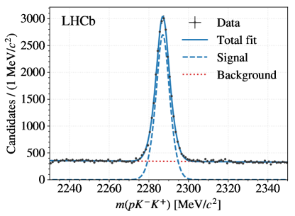
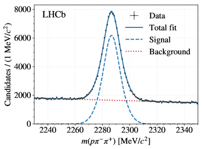
Figure 1: The $ph^{-}h^{+}$ invariant mass spectra from the fully selected ${\mathchar 28931\relax}_{{c}}^{+}\!\rightarrow p{{K}^{-}}{{K}^{+}}$ (left) and ${\mathchar 28931\relax}_{{c}}^{+}\!\rightarrow p{{\pi}^{-}}{{\pi}^{+}}$ (right) datasets summed over all data-taking conditions. The results of the fit to each dataset are shown for illustration. The widths of the signal distributions differ due to the different $Q$-value between the two decays, where the larger value for the ${\mathchar 28931\relax}_{{c}}^{+}\!\rightarrow p{{\pi}^{-}}{{\pi}^{+}}$ mode results in a broader shape.

Table 1: Signal yields measured in the fit for each of the four subsets of the $p{{K}^{-}}{{K}^{+}}$ and $p{{\pi}^{-}}{{\pi}^{+}}$ data (two centre-of-mass energies, 7 and $8\text{\,}\mathrm{TeV}$, and two polarities of the dipole magnet, up and down). The corresponding integrated luminosity of each subset is also given.

$\sqrt{s}$	Polarity	Int. lumi. [pb-1]	$p{{K}^{-}}{{K}^{+}}$ yield	$p{{\pi}^{-}}{{\pi}^{+}}$ yield
$7\,$TeV	Up	$422$ p m 7	$2880$ p m 70	$18\,450$ p m 190
$7\,$TeV	Down	$563$ p m 9	$3940$ p m 80	$25\,130$ p m 230
$8\,$TeV	Up	$1000$ p m 11	$9040$ p m 120	$57\,730$ p m 350
$8\,$TeV	Down	$992$ p m 11	$9330$ p m 120	$60\,080$ p m 360

To measure $A_{\text{raw}}$ as in Eq. 2, each data subsample is split by proton charge into ${\mathchar 28931\relax}_{{c}}^{+}$ and ${\kern 1.00006pt\overline{\kern-1.00006pt\mathchar 28931\relax}}_{{c}}^{-}$ subsets. The model used in the previously described fit is used to define charge-dependent models, where the parameter vectors of each model, $\xi^{+}$ and $\xi^{-}$, are independent. Rather than fitting charge-dependent signal and background yields directly, however, they are parameterised using the total number of signal and background candidates, $N_{\text{Sig}}$ and $N_{\text{Bkg}}$, and the signal and background asymmetries, $A_{\text{raw}}$ and $A_{\text{raw}}^{\text{Bkg}}$,

$$N_{\text{Sig}}^{\pm} =\frac{1}{2}N_{\text{Sig}}(1\pm A_{\text{raw}}),$$ (9)

$$N_{\text{Bkg}}^{\pm} =\frac{1}{2}N_{\text{Bkg}}(1\pm A_{\text{raw}}^{\text{Bkg}}).$$ (10)

The addition of per-candidate weights, which are described in the following section, requires a cost function that uses the sum of weights in each bin, rather than the count as in Eq. 8, defined as

$$\chi^{2}=\sum_{i=1}^{B}\left[\frac{(W_{i}^{+}-N^{+}f_{\text{Tot}}^{+}(m_{i};\xi^{+}))^{2}}{(\delta{}W_{i}^{+})^{2}}+\frac{(W_{i}^{-}-N^{-}f_{\text{Tot}}^{-}(m_{i};\xi^{-}))^{2}}{(\delta{}W_{i}^{-})^{2}}\right],$$ (11)

where $W_{i}^{\pm}$ is the sum of the weights of candidates in the $i$th bin in the ${\mathchar 28931\relax}_{{c}}^{\pm}$ sample, and $\delta{}W_{i}^{\pm}$ is the uncertainty on that sum.

5 Kinematic and efficiency corrections

The experimental asymmetries listed in Eq. 3 are specific to the production environment at the LHC and the construction of the LHCb detector, and so their cancellation in $\Delta A_{{C\!P}}^{\text{wgt}}$ is crucial in providing an unbiased measurement. This section presents the statistical methods used to compute the kinematic and efficiency corrections, which are evaluated as per-candidate weights to be used in the simultaneous $\chi^{2}$ fit previously described.

5.1 Kinematic weighting

The production and detection asymmetries depend on the kinematics of the particles involved. If the ${\mathchar 28931\relax}^{0}_{b}$, muon, and proton kinematic spectra are the same between the $p{{K}^{-}}{{K}^{+}}$ and $p{{\pi}^{-}}{{\pi}^{+}}$ data, then the ${\mathchar 28931\relax}^{0}_{b}$ production asymmetry and muon and proton detection asymmetries will cancel in $\Delta A_{{C\!P}}^{\text{wgt}}$. If the $h^{-}$ and $h^{+}$ kinematics are equal within each separate $p{{K}^{-}}{{K}^{+}}$ and $p{{\pi}^{-}}{{\pi}^{+}}$ sample, then the kaon ($f=p{{K}^{-}}{{K}^{+}}$) or pion ($f=p{{\pi}^{-}}{{\pi}^{+}}$) detection asymmetries will cancel in $A_{\text{raw}}(f)$. The $h^{-}$ kinematics agree well with the $h^{+}$ spectra in the data, but the ${\mathchar 28931\relax}^{0}_{b}$, muon, and proton kinematics do not, and so a per-candidate weighting technique is employed to match the kinematic spectra of the $p{{\pi}^{-}}{{\pi}^{+}}{\mu^{-}}$ state to those of the $p{{K}^{-}}{{K}^{+}}{\mu^{-}}$ state.

To compute the per-candidate weights, a forest of shallow decision trees with gradient boosting (a GBDT) is used [25, 26, 27]. This method recursively bins the $p{{K}^{-}}{{K}^{+}}$ and $p{{\pi}^{-}}{{\pi}^{+}}$ input data such that regions with larger differences between the two samples are more finely partitioned. After fitting, each $p{{\pi}^{-}}{{\pi}^{+}}$ candidate is assigned a weight $d$. To reduce biases that may result from overfitting, where the GBDT model becomes sensitive to the statistical fluctuations in the input data, the data are split in two, and independent GBDTs are fitted to each subset. The GBDT built with one half of the data is used to evaluate weights for the other half, and vice versa.

The ${\mathchar 28931\relax}_{{c}}^{+}$ and proton $p_{\mathrm{T}}$ and pseudorapidity for each $p{{K}^{-}}{{K}^{+}}$ and $p{{\pi}^{-}}{{\pi}^{+}}$ candidate are used as input to the GBDT. The ${\mathchar 28931\relax}_{{c}}^{+}$ kinematics are chosen since the large boost in the laboratory frame induces a large correlation with ${\mathchar 28931\relax}^{0}_{b}$ and muon kinematics. An agreement in the ${\mathchar 28931\relax}_{{c}}^{+}$ kinematics therefore results in an agreement in the ${\mathchar 28931\relax}^{0}_{b}$ and muon spectra. The proton kinematics are chosen as the different $Q$ values of the decays will a priori result in different proton spectra.

The ${\mathchar 28931\relax}^{0}_{b}$, muon, proton, and $h^{-}$/$h^{+}$ kinematics agree well after weighting, as demonstrated for a subset of kinematic variables in Fig. 2. Any remaining differences will result in residual asymmetries in $\Delta A_{{C\!P}}^{\text{wgt}}$, and the presence of these differences is studied in the context of systematic effects as described in Section 6.

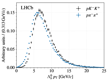
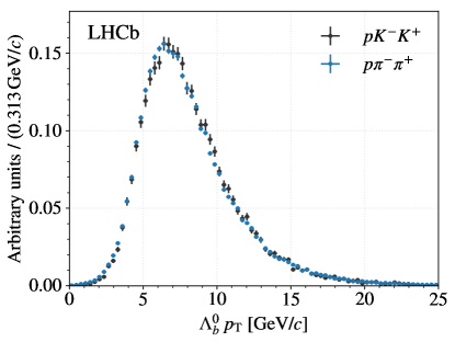
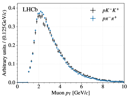
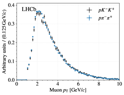
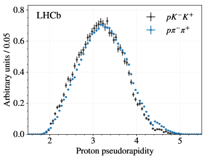
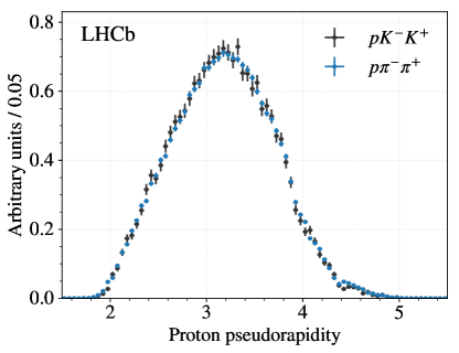
Figure 2: Background-subtracted distributions of the ${\mathchar 28931\relax}^{0}_{b}$ candidate transverse momentum (top row), the muon candidate transverse momentum (middle row), and the proton candidate pseudorapidity (bottom row) both before (left column) and after (right column) weighting the $p{{\pi}^{-}}{{\pi}^{+}}$ sample (blue points) to match the $p{{K}^{-}}{{K}^{+}}$ sample (black points). The data are summed across all data-taking conditions.

5.2 Efficiency corrections

The acceptance, reconstruction, and selection efficiencies as a function of the 5D $ph^{-}h^{+}$ phase space are also modelled using GBDTs. Simulated events are generated with a uniform ${\mathchar 28931\relax}_{{c}}^{+}\!\rightarrow ph^{-}h^{+}$ matrix element and used as input to the training, sampled before and after the detector acceptance and data processing steps. One- and two-dimensional efficiency estimates are made as histogram ratios of the before and after data, and projections of the efficiency model obtained using the simulation agrees well with these. The model is then used to predict per-candidate efficiencies in the data.

5.3 Use in determining $A_{\text{raw}}$

The cost function in Eq. 11 uses the sum of per-candidate weights in each bin and its uncertainty. The weights are defined using the kinematic weight $d_{j}$, equal to unity for ${\mathchar 28931\relax}_{{c}}^{+}\!\rightarrow p{{K}^{-}}{{K}^{+}}$ candidates, and the efficiency correction $\varepsilon_{j}$ of the $j$th candidate in the $i$th $m(ph^{-}h^{+})$ bin,

$$W_{i}=W\sum_{j=1}^{N_{i}}\frac{d_{j}}{\varepsilon_{j}},\quad\delta{}W_{i}^{2}=W_{i},$$ (12)

where the normalisation factor $W$ is defined as

$$W=\frac{\sum_{j=1}^{N_{i}}\frac{d_{j}}{\varepsilon_{j}}}{\sum_{j=1}^{N_{i}}\left(\frac{d_{j}}{\varepsilon_{j}}\right)^{2}}.$$ (13)

The term $W_{i}$ can be called the number of ‘effective’ entries in the bin, as it encodes the size of an unweighted data sample with the same statistical power as the weighted sample. For the $p{{\pi}^{-}}{{\pi}^{+}}$ data, which is weighted to match the $p{{K}^{-}}{{K}^{+}}$ kinematics, the effective sample size is around $80\text{\,}\mathrm{\char 37\relax}$ that of the unweighted $p{{\pi}^{-}}{{\pi}^{+}}$ sample. The weighted data are shown in the $m^{2}({p}h^{-})$–$m^{2}(h^{-}h^{+})$ plane in Fig. 3.

The statistical treatment of the weights in the fit is validated by randomly sorting candidates into ${\mathchar 28931\relax}_{{c}}^{+}$ and ${\kern 1.00006pt\overline{\kern-1.00006pt\mathchar 28931\relax}}_{{c}}^{-}$ datasets and fitting the model 500 times, where it is seen that the distribution of $A_{\text{raw}}(f)$ divided by its uncertainty is centred around zero, the expected value, and has a standard deviation of 1, indicating that the error estimate is correct.

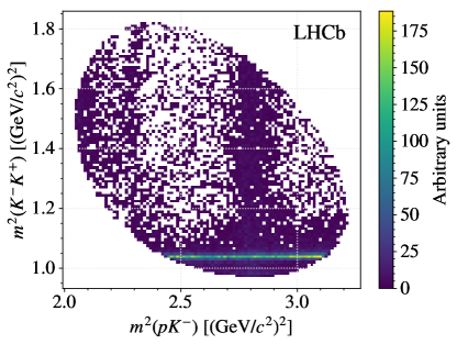
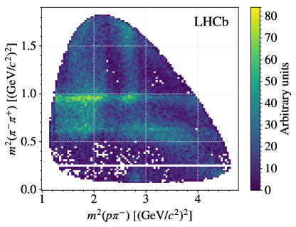
Figure 3: Background-subtracted and efficiency-corrected ${\mathchar 28931\relax}_{{c}}^{+}\!\rightarrow p{{K}^{-}}{{K}^{+}}$ (left) and ${\mathchar 28931\relax}_{{c}}^{+}\!\rightarrow p{{\pi}^{-}}{{\pi}^{+}}$ (right) data in the $m^{2}({p}h^{-})$–$m^{2}(h^{-}h^{+})$ plane, integrated across all data-taking subsamples. The $p{{K}^{-}}{{K}^{+}}$ data feature a prominent $\phi\!\rightarrow{{K}^{-}}{{K}^{+}}$ component, whilst the $p{{\pi}^{-}}{{\pi}^{+}}$ data exhibit $\rho(770)/\omega(782)\!\rightarrow{{\pi}^{-}}{{\pi}^{+}}$ and $f_{0}(980)\!\rightarrow{{\pi}^{-}}{{\pi}^{+}}$ components.

6 Systematic effects

To evaluate possible biases on the measurement of $\Delta A_{{C\!P}}^{\text{wgt}}$ due to systematic effects, several studies are performed and deviations from the nominal results are computed. Statistically significant deviations are assigned to the measurement as systematic uncertainties.

The model used in the simultaneous $\chi^{2}$ fit, described in Section 4, is derived empirically, and there may be other models which described the data similarly well. Variations of the choice of background model are found to have a negligible effect on the measurement of $\Delta A_{{C\!P}}^{\text{wgt}}$, however different signal models can change the results significantly. To assess an associated systematic uncertainty based on the choice of signal model, the signal ${\mathchar 28931\relax}_{{c}}^{+}$ and ${\kern 1.00006pt\overline{\kern-1.00006pt\mathchar 28931\relax}}_{{c}}^{-}$ yields are determined using the method of sideband subtraction. Here, data from the regions on either side of the ${\mathchar 28931\relax}_{{c}}^{\pm}$ signal peak are assumed to be linearly distributed and are used to approximate the background yield in the peak region. Given that the data used for sideband subtraction are the same as for the nominal $\chi^{2}$ fit, the measurements using the two techniques are assumed to be fully correlated, such that even small differences between them are statistically significant. On the average of $\Delta A_{{C\!P}}^{\text{wgt}}$, taken across all data-taking conditions, a difference of $0.2\text{\,}\mathrm{\char 37\relax}$ is seen with respect to the average of the results using the full fit, and this difference is assigned as a systematic uncertainty.

The kinematic weighting procedure defined in Section 5 can only equalise the $p{{K}^{-}}{{K}^{+}}{\mu^{-}}$ and $p{{\pi}^{-}}{{\pi}^{+}}{\mu^{-}}$ kinematics approximately, and so residual differences will remain. These differences can cause a bias on $\Delta A_{{C\!P}}^{\text{wgt}}$, with a size depending on the size of the relevant asymmetry. Measurements of the ${\mathchar 28931\relax}^{0}_{b}$ production asymmetry and the muon, kaon, and pion detection asymmetries using LHCb data exist [8, 9, 5, 10], and estimates of the proton detection asymmetry using simulated events have been used previously [8], and so the measurement of $\Delta A_{{C\!P}}^{\text{wgt}}$ can be corrected for directly. The correction is found to be less than one per mille, but with a relative uncertainty of $20\text{\,}\mathrm{\char 37\relax}$, and so a systematic uncertainty of $0.1\text{\,}\mathrm{\char 37\relax}$ is assigned to $\Delta A_{{C\!P}}^{\text{wgt}}$.

The limited size of the simulated sample results in a statistical uncertainty on the efficiencies taken from the phase space efficiency model. The size of this uncertainty is evaluated by resampling the simulated data 500 times, each time building a new model and computing the efficiencies of the data using that model. The simultaneous $\chi^{2}$ fit to measure $A_{\text{raw}}(f)$ is then performed for each set of efficiencies, resulting in a spread of values of $\Delta A_{{C\!P}}^{\text{wgt}}$ with a standard deviation of $0.57\text{\,}\mathrm{\char 37\relax}$, which is taken as the systematic uncertainty due to the limited simulated sample size.

Due to the presence of ${\mathchar 28931\relax}_{{c}}^{+}$ decays originating from sources other than ${{\mathchar 28931\relax}^{0}_{b}}\!\rightarrow{\mathchar 28931\relax}_{{c}}^{+}{\mu^{-}}{}X$ decays, such as directly from the PV or from other $b$-hadron decays, the measurement may be biased, as such sources can carry different experimental asymmetries. The composition of the data sample is inferred from the reconstructed ${\mathchar 28931\relax}^{0}_{b}$ mass and from the impact parameter distribution of the ${\mathchar 28931\relax}_{{c}}^{+}$ vertex. The latter is seen to be consistent with that for ${\mathchar 28931\relax}_{{c}}^{+}$ produced exclusively in $b$-hadron decays, whilst the former is consistent between $p{{K}^{-}}{{K}^{+}}$ and $p{{\pi}^{-}}{{\pi}^{+}}$ samples, such that asymmetries from other sources will cancel in $\Delta A_{{C\!P}}^{\text{wgt}}$. Any associated systematic uncertainty is assumed to be negligible.

The total systematic uncertainty is found to be $0.61\text{\,}\mathrm{\char 37\relax}$, computed as the sum in quadrature of the individual uncertainties. These are assumed to be uncorrelated and are summarised in Table 2.

Table 2: Systematic uncertainties on $\Delta A_{{C\!P}}^{\text{wgt}}$ and their magnitudes. The dash indicates that the uncertainty is assessed to be negligible.

Source Uncertainty [$\mathrm{\char 37\relax}$] Fit signal model $0.20$ Fit background model — Residual asymmetries $0.10$ Limited simulated sample size $0.57$ Prompt ${\mathchar 28931\relax}_{{c}}^{+}$ — Total $0.61$

7 Results

The value of $A_{\text{raw}}(f)$ is found for each final state and data-taking condition separately, and for a given centre-of-mass energy is taken as the arithematic average of the polarity-dependent measurements. The average across $\sqrt{s}=$7\text{\,}\mathrm{TeV}$$ and $8\text{\,}\mathrm{TeV}$ is made by weighting the measurements by their variances. The asymmetries for $p{{K}^{-}}{{K}^{+}}$ and $p{{\pi}^{-}}{{\pi}^{+}}$ are measured to be

$$A_{\text{raw}}(p{{K}^{-}}{{K}^{+}}) =$3.72\pm 0.78\text{\,}\mathrm{\char 37\relax}$,$$

$$A_{\text{raw}}^{\text{wgt}}(p{{\pi}^{-}}{{\pi}^{+}}) =$3.42\pm 0.47\text{\,}\mathrm{\char 37\relax}$.$$

where the uncertainties are statistical and take into account the reduction in statistical power due to the weighting. The difference is

$$\Delta A_{{C\!P}}^{\text{wgt}}=(0.30\pm 0.91\pm 0.61)$\mathrm{\char 37\relax}$,$$

where the first uncertainty is statistical and the second is systematic. The measurements of $A_{\text{raw}}(p{{K}^{-}}{{K}^{+}})$, $A_{\text{raw}}^{\text{wgt}}(p{{\pi}^{-}}{{\pi}^{+}})$, and $\Delta A_{{C\!P}}^{\text{wgt}}$ as a function of data-taking conditions are presented in Fig. 4.

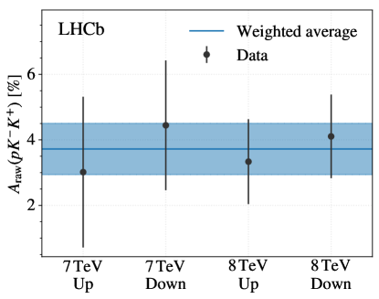
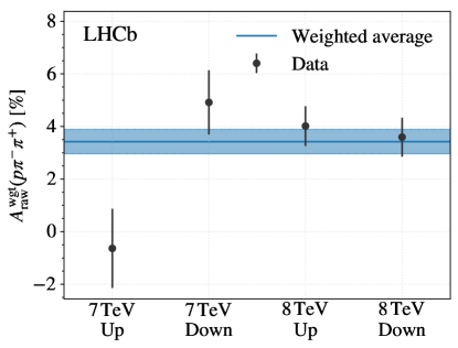
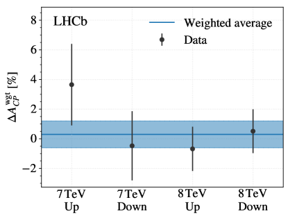
Figure 4: Values of and statistical uncertainties on the asymmetries $A_{\text{raw}}(p{{K}^{-}}{{K}^{+}})$ (top left), $A_{\text{raw}}^{\text{wgt}}(p{{\pi}^{-}}{{\pi}^{+}})$ (top right), and $\Delta A_{{C\!P}}^{\text{wgt}}$ (bottom centre), for the four data subsamples (two centre-of-mass energies, 7 and $8\text{\,}\mathrm{TeV}$, and two polarities of the dipole magnet, up and down). For each asymmetry, the average of the four data points, as described in the text, is also shown, where the band indicates the uncertainty.

8 Summary

The raw $C\!P$ asymmetries in the decays ${\mathchar 28931\relax}_{{c}}^{+}\!\rightarrow p{{K}^{-}}{{K}^{+}}$ and $p{{\pi}^{-}}{{\pi}^{+}}$ are measured using ${{\mathchar 28931\relax}^{0}_{b}}\!\rightarrow{\mathchar 28931\relax}_{{c}}^{+}{\mu^{-}}{}X$ decays. Kinematics in the $p{{\pi}^{-}}{{\pi}^{+}}$ data are weighted to match those in the $p{{K}^{-}}{{K}^{+}}$ data, such that the effect of experimental asymmetries on the $C\!P$ asymmetry parameter $\Delta A_{{C\!P}}^{\text{wgt}}$ is negligible. Acceptance, reconstruction, and selection efficiencies across the five-dimensional $ph^{-}h^{+}$ phase space are corrected for. Systematic effects arising from the mass distribution modelling, imperfect kinematic weighting, finite simulated sample size, and the inclusion of ${\mathchar 28931\relax}_{{c}}^{+}$ decays from sources other than ${{\mathchar 28931\relax}^{0}_{b}}\!\rightarrow{\mathchar 28931\relax}_{{c}}^{+}{\mu^{-}}{}X$ decays are considered. The total systematic uncertainty assigned to these effects is smaller than the statistical uncertainty on $\Delta A_{{C\!P}}^{\text{wgt}}$, whose central value is measured to be consistent with zero.

This analysis constitutes the first measurement of a $C\!P$ violation parameter in three-body ${\mathchar 28931\relax}_{{c}}^{+}$ decays, but more data is required to match the sensitivity of similar measurements using charm mesons. Further studies into the structure of the $ph^{-}h^{+}$ phase space, across which $C\!P$-violating effects may strongly vary, would be beneficial as input to theoretical calculations.

LHCb collaboration

R. Aaij⁴⁰, B. Adeva³⁹, M. Adinolfi⁴⁸, Z. Ajaltouni⁵, S. Akar⁵⁹, J. Albrecht¹⁰, F. Alessio⁴⁰, M. Alexander⁵³, A. Alfonso Albero³⁸, S. Ali⁴³, G. Alkhazov³¹, P. Alvarez Cartelle⁵⁵, A.A. Alves Jr⁵⁹, S. Amato², S. Amerio²³, Y. Amhis⁷, L. An³, L. Anderlini¹⁸, G. Andreassi⁴¹, M. Andreotti^17,g, J.E. Andrews⁶⁰, R.B. Appleby⁵⁶, F. Archilli⁴³, P. d’Argent¹², J. Arnau Romeu⁶, A. Artamonov³⁷, M. Artuso⁶¹, E. Aslanides⁶, M. Atzeni⁴², G. Auriemma²⁶, M. Baalouch⁵, I. Babuschkin⁵⁶, S. Bachmann¹², J.J. Back⁵⁰, A. Badalov^38,m, C. Baesso⁶², S. Baker⁵⁵, V. Balagura^7,b, W. Baldini¹⁷, A. Baranov³⁵, R.J. Barlow⁵⁶, C. Barschel⁴⁰, S. Barsuk⁷, W. Barter⁵⁶, F. Baryshnikov³², V. Batozskaya²⁹, V. Battista⁴¹, A. Bay⁴¹, L. Beaucourt⁴, J. Beddow⁵³, F. Bedeschi²⁴, I. Bediaga¹, A. Beiter⁶¹, L.J. Bel⁴³, N. Beliy⁶³, V. Bellee⁴¹, N. Belloli^21,i, K. Belous³⁷, I. Belyaev^32,40, E. Ben-Haim⁸, G. Bencivenni¹⁹, S. Benson⁴³, S. Beranek⁹, A. Berezhnoy³³, R. Bernet⁴², D. Berninghoff¹², E. Bertholet⁸, A. Bertolin²³, C. Betancourt⁴², F. Betti¹⁵, M.O. Bettler⁴⁰, M. van Beuzekom⁴³, Ia. Bezshyiko⁴², S. Bifani⁴⁷, P. Billoir⁸, A. Birnkraut¹⁰, A. Bizzeti^18,u, M. Bjørn⁵⁷, T. Blake⁵⁰, F. Blanc⁴¹, S. Blusk⁶¹, V. Bocci²⁶, T. Boettcher⁵⁸, A. Bondar^36,w, N. Bondar³¹, I. Bordyuzhin³², S. Borghi^56,40, M. Borisyak³⁵, M. Borsato³⁹, F. Bossu⁷, M. Boubdir⁹, T.J.V. Bowcock⁵⁴, E. Bowen⁴², C. Bozzi^17,40, S. Braun¹², J. Brodzicka²⁷, D. Brundu¹⁶, E. Buchanan⁴⁸, C. Burr⁵⁶, A. Bursche^16,f, J. Buytaert⁴⁰, W. Byczynski⁴⁰, S. Cadeddu¹⁶, H. Cai⁶⁴, R. Calabrese^17,g, R. Calladine⁴⁷, M. Calvi^21,i, M. Calvo Gomez^38,m, A. Camboni^38,m, P. Campana¹⁹, D.H. Campora Perez⁴⁰, L. Capriotti⁵⁶, A. Carbone^15,e, G. Carboni^25,j, R. Cardinale^20,h, A. Cardini¹⁶, P. Carniti^21,i, L. Carson⁵², K. Carvalho Akiba², G. Casse⁵⁴, L. Cassina²¹, M. Cattaneo⁴⁰, G. Cavallero^20,40,h, R. Cenci^24,t, D. Chamont⁷, M.G. Chapman⁴⁸, M. Charles⁸, Ph. Charpentier⁴⁰, G. Chatzikonstantinidis⁴⁷, M. Chefdeville⁴, S. Chen¹⁶, S.F. Cheung⁵⁷, S.-G. Chitic⁴⁰, V. Chobanova³⁹, M. Chrzaszcz⁴², A. Chubykin³¹, P. Ciambrone¹⁹, X. Cid Vidal³⁹, G. Ciezarek⁴⁰, P.E.L. Clarke⁵², M. Clemencic⁴⁰, H.V. Cliff⁴⁹, J. Closier⁴⁰, V. Coco⁴⁰, J. Cogan⁶, E. Cogneras⁵, V. Cogoni^16,f, L. Cojocariu³⁰, P. Collins⁴⁰, T. Colombo⁴⁰, A. Comerma-Montells¹², A. Contu¹⁶, G. Coombs⁴⁰, S. Coquereau³⁸, G. Corti⁴⁰, M. Corvo^17,g, C.M. Costa Sobral⁵⁰, B. Couturier⁴⁰, G.A. Cowan⁵², D.C. Craik⁵⁸, A. Crocombe⁵⁰, M. Cruz Torres¹, R. Currie⁵², C. D’Ambrosio⁴⁰, F. Da Cunha Marinho², C.L. Da Silva⁷³, E. Dall’Occo⁴³, J. Dalseno⁴⁸, A. Davis³, O. De Aguiar Francisco⁴⁰, K. De Bruyn⁴⁰, S. De Capua⁵⁶, M. De Cian¹², J.M. De Miranda¹, L. De Paula², M. De Serio^14,d, P. De Simone¹⁹, C.T. Dean⁵³, D. Decamp⁴, L. Del Buono⁸, H.-P. Dembinski¹¹, M. Demmer¹⁰, A. Dendek²⁸, D. Derkach³⁵, O. Deschamps⁵, F. Dettori⁵⁴, B. Dey⁶⁵, A. Di Canto⁴⁰, P. Di Nezza¹⁹, H. Dijkstra⁴⁰, F. Dordei⁴⁰, M. Dorigo⁴⁰, A. Dosil Suárez³⁹, L. Douglas⁵³, A. Dovbnya⁴⁵, K. Dreimanis⁵⁴, L. Dufour⁴³, G. Dujany⁸, P. Durante⁴⁰, J.M. Durham⁷³, D. Dutta⁵⁶, R. Dzhelyadin³⁷, M. Dziewiecki¹², A. Dziurda⁴⁰, A. Dzyuba³¹, S. Easo⁵¹, M. Ebert⁵², U. Egede⁵⁵, V. Egorychev³², S. Eidelman^36,w, S. Eisenhardt⁵², U. Eitschberger¹⁰, R. Ekelhof¹⁰, L. Eklund⁵³, S. Ely⁶¹, S. Esen¹², H.M. Evans⁴⁹, T. Evans⁵⁷, A. Falabella¹⁵, N. Farley⁴⁷, S. Farry⁵⁴, D. Fazzini^21,i, L. Federici²⁵, D. Ferguson⁵², G. Fernandez³⁸, P. Fernandez Declara⁴⁰, A. Fernandez Prieto³⁹, F. Ferrari¹⁵, L. Ferreira Lopes⁴¹, F. Ferreira Rodrigues², M. Ferro-Luzzi⁴⁰, S. Filippov³⁴, R.A. Fini¹⁴, M. Fiorini^17,g, M. Firlej²⁸, C. Fitzpatrick⁴¹, T. Fiutowski²⁸, F. Fleuret^7,b, M. Fontana^16,40, F. Fontanelli^20,h, R. Forty⁴⁰, V. Franco Lima⁵⁴, M. Frank⁴⁰, C. Frei⁴⁰, J. Fu^22,q, W. Funk⁴⁰, E. Furfaro^25,j, C. Färber⁴⁰, E. Gabriel⁵², A. Gallas Torreira³⁹, D. Galli^15,e, S. Gallorini²³, S. Gambetta⁵², M. Gandelman², P. Gandini²², Y. Gao³, L.M. Garcia Martin⁷¹, J. García Pardiñas³⁹, J. Garra Tico⁴⁹, L. Garrido³⁸, D. Gascon³⁸, C. Gaspar⁴⁰, L. Gavardi¹⁰, G. Gazzoni⁵, D. Gerick¹², E. Gersabeck⁵⁶, M. Gersabeck⁵⁶, T. Gershon⁵⁰, Ph. Ghez⁴, S. Gianì⁴¹, V. Gibson⁴⁹, O.G. Girard⁴¹, L. Giubega³⁰, K. Gizdov⁵², V.V. Gligorov⁸, D. Golubkov³², A. Golutvin^55,69,y, A. Gomes^1,a, I.V. Gorelov³³, C. Gotti^21,i, E. Govorkova⁴³, J.P. Grabowski¹², R. Graciani Diaz³⁸, L.A. Granado Cardoso⁴⁰, E. Graugés³⁸, E. Graverini⁴², G. Graziani¹⁸, A. Grecu³⁰, R. Greim⁹, P. Griffith¹⁶, L. Grillo⁵⁶, L. Gruber⁴⁰, B.R. Gruberg Cazon⁵⁷, O. Grünberg⁶⁷, E. Gushchin³⁴, Yu. Guz³⁷, T. Gys⁴⁰, C. Göbel⁶², T. Hadavizadeh⁵⁷, C. Hadjivasiliou⁵, G. Haefeli⁴¹, C. Haen⁴⁰, S.C. Haines⁴⁹, B. Hamilton⁶⁰, X. Han¹², T.H. Hancock⁵⁷, S. Hansmann-Menzemer¹², N. Harnew⁵⁷, S.T. Harnew⁴⁸, C. Hasse⁴⁰, M. Hatch⁴⁰, J. He⁶³, M. Hecker⁵⁵, K. Heinicke¹⁰, A. Heister⁹, K. Hennessy⁵⁴, P. Henrard⁵, L. Henry⁷¹, E. van Herwijnen⁴⁰, M. Heß⁶⁷, A. Hicheur², D. Hill⁵⁷, P.H. Hopchev⁴¹, W. Hu⁶⁵, W. Huang⁶³, Z.C. Huard⁵⁹, W. Hulsbergen⁴³, T. Humair⁵⁵, M. Hushchyn³⁵, D. Hutchcroft⁵⁴, P. Ibis¹⁰, M. Idzik²⁸, P. Ilten⁴⁷, R. Jacobsson⁴⁰, J. Jalocha⁵⁷, E. Jans⁴³, A. Jawahery⁶⁰, F. Jiang³, M. John⁵⁷, D. Johnson⁴⁰, C.R. Jones⁴⁹, C. Joram⁴⁰, B. Jost⁴⁰, N. Jurik⁵⁷, S. Kandybei⁴⁵, M. Karacson⁴⁰, J.M. Kariuki⁴⁸, S. Karodia⁵³, N. Kazeev³⁵, M. Kecke¹², F. Keizer⁴⁹, M. Kelsey⁶¹, M. Kenzie⁴⁹, T. Ketel⁴⁴, E. Khairullin³⁵, B. Khanji¹², C. Khurewathanakul⁴¹, T. Kirn⁹, S. Klaver¹⁹, K. Klimaszewski²⁹, T. Klimkovich¹¹, S. Koliiev⁴⁶, M. Kolpin¹², R. Kopecna¹², P. Koppenburg⁴³, A. Kosmyntseva³², S. Kotriakhova³¹, M. Kozeiha⁵, L. Kravchuk³⁴, M. Kreps⁵⁰, F. Kress⁵⁵, P. Krokovny^36,w, W. Krzemien²⁹, W. Kucewicz^27,l, M. Kucharczyk²⁷, V. Kudryavtsev^36,w, A.K. Kuonen⁴¹, T. Kvaratskheliya^32,40, D. Lacarrere⁴⁰, G. Lafferty⁵⁶, A. Lai¹⁶, G. Lanfranchi¹⁹, C. Langenbruch⁹, T. Latham⁵⁰, C. Lazzeroni⁴⁷, R. Le Gac⁶, A. Leflat^33,40, J. Lefrançois⁷, R. Lefèvre⁵, F. Lemaitre⁴⁰, E. Lemos Cid³⁹, O. Leroy⁶, T. Lesiak²⁷, B. Leverington¹², P.-R. Li⁶³, T. Li³, Y. Li⁷, Z. Li⁶¹, X. Liang⁶¹, T. Likhomanenko⁶⁸, R. Lindner⁴⁰, F. Lionetto⁴², V. Lisovskyi⁷, X. Liu³, D. Loh⁵⁰, A. Loi¹⁶, I. Longstaff⁵³, J.H. Lopes², D. Lucchesi^23,o, M. Lucio Martinez³⁹, H. Luo⁵², A. Lupato²³, E. Luppi^17,g, O. Lupton⁴⁰, A. Lusiani²⁴, X. Lyu⁶³, F. Machefert⁷, F. Maciuc³⁰, V. Macko⁴¹, P. Mackowiak¹⁰, S. Maddrell-Mander⁴⁸, O. Maev^31,40, K. Maguire⁵⁶, D. Maisuzenko³¹, M.W. Majewski²⁸, S. Malde⁵⁷, B. Malecki²⁷, A. Malinin⁶⁸, T. Maltsev^36,w, G. Manca^16,f, G. Mancinelli⁶, D. Marangotto^22,q, J. Maratas^5,v, J.F. Marchand⁴, U. Marconi¹⁵, C. Marin Benito³⁸, M. Marinangeli⁴¹, P. Marino⁴¹, J. Marks¹², G. Martellotti²⁶, M. Martin⁶, M. Martinelli⁴¹, D. Martinez Santos³⁹, F. Martinez Vidal⁷¹, A. Massafferri¹, R. Matev⁴⁰, A. Mathad⁵⁰, Z. Mathe⁴⁰, C. Matteuzzi²¹, A. Mauri⁴², E. Maurice^7,b, B. Maurin⁴¹, A. Mazurov⁴⁷, M. McCann^55,40, A. McNab⁵⁶, R. McNulty¹³, J.V. Mead⁵⁴, B. Meadows⁵⁹, C. Meaux⁶, F. Meier¹⁰, N. Meinert⁶⁷, D. Melnychuk²⁹, M. Merk⁴³, A. Merli^22,40,q, E. Michielin²³, D.A. Milanes⁶⁶, E. Millard⁵⁰, M.-N. Minard⁴, L. Minzoni¹⁷, D.S. Mitzel¹², A. Mogini⁸, J. Molina Rodriguez¹, T. Mombächer¹⁰, I.A. Monroy⁶⁶, S. Monteil⁵, M. Morandin²³, M.J. Morello^24,t, O. Morgunova⁶⁸, J. Moron²⁸, A.B. Morris⁵², R. Mountain⁶¹, F. Muheim⁵², M. Mulder⁴³, D. Müller⁵⁶, J. Müller¹⁰, K. Müller⁴², V. Müller¹⁰, P. Naik⁴⁸, T. Nakada⁴¹, R. Nandakumar⁵¹, A. Nandi⁵⁷, I. Nasteva², M. Needham⁵², N. Neri^22,40, S. Neubert¹², N. Neufeld⁴⁰, M. Neuner¹², T.D. Nguyen⁴¹, C. Nguyen-Mau^41,n, S. Nieswand⁹, R. Niet¹⁰, N. Nikitin³³, T. Nikodem¹², A. Nogay⁶⁸, D.P. O’Hanlon⁵⁰, A. Oblakowska-Mucha²⁸, V. Obraztsov³⁷, S. Ogilvy¹⁹, R. Oldeman^16,f, C.J.G. Onderwater⁷², A. Ossowska²⁷, J.M. Otalora Goicochea², P. Owen⁴², A. Oyanguren⁷¹, P.R. Pais⁴¹, A. Palano¹⁴, M. Palutan^19,40, A. Papanestis⁵¹, M. Pappagallo⁵², L.L. Pappalardo^17,g, W. Parker⁶⁰, C. Parkes⁵⁶, G. Passaleva^18,40, A. Pastore^14,d, M. Patel⁵⁵, C. Patrignani^15,e, A. Pearce⁴⁰, A. Pellegrino⁴³, G. Penso²⁶, M. Pepe Altarelli⁴⁰, S. Perazzini⁴⁰, D. Pereima³², P. Perret⁵, L. Pescatore⁴¹, K. Petridis⁴⁸, A. Petrolini^20,h, A. Petrov⁶⁸, M. Petruzzo^22,q, E. Picatoste Olloqui³⁸, B. Pietrzyk⁴, G. Pietrzyk⁴¹, M. Pikies²⁷, D. Pinci²⁶, F. Pisani⁴⁰, A. Pistone^20,h, A. Piucci¹², V. Placinta³⁰, S. Playfer⁵², M. Plo Casasus³⁹, F. Polci⁸, M. Poli Lener¹⁹, A. Poluektov⁵⁰, I. Polyakov⁶¹, E. Polycarpo², G.J. Pomery⁴⁸, S. Ponce⁴⁰, A. Popov³⁷, D. Popov^11,40, S. Poslavskii³⁷, C. Potterat², E. Price⁴⁸, J. Prisciandaro³⁹, C. Prouve⁴⁸, V. Pugatch⁴⁶, A. Puig Navarro⁴², H. Pullen⁵⁷, G. Punzi^24,p, W. Qian⁵⁰, J. Qin⁶³, R. Quagliani⁸, B. Quintana⁵, B. Rachwal²⁸, J.H. Rademacker⁴⁸, M. Rama²⁴, M. Ramos Pernas³⁹, M.S. Rangel², I. Raniuk^45,†, F. Ratnikov^35,x, G. Raven⁴⁴, M. Ravonel Salzgeber⁴⁰, M. Reboud⁴, F. Redi⁴¹, S. Reichert¹⁰, A.C. dos Reis¹, C. Remon Alepuz⁷¹, V. Renaudin⁷, S. Ricciardi⁵¹, S. Richards⁴⁸, M. Rihl⁴⁰, K. Rinnert⁵⁴, P. Robbe⁷, A. Robert⁸, A.B. Rodrigues⁴¹, E. Rodrigues⁵⁹, J.A. Rodriguez Lopez⁶⁶, A. Rogozhnikov³⁵, S. Roiser⁴⁰, A. Rollings⁵⁷, V. Romanovskiy³⁷, A. Romero Vidal^39,40, M. Rotondo¹⁹, M.S. Rudolph⁶¹, T. Ruf⁴⁰, P. Ruiz Valls⁷¹, J. Ruiz Vidal⁷¹, J.J. Saborido Silva³⁹, E. Sadykhov³², N. Sagidova³¹, B. Saitta^16,f, V. Salustino Guimaraes⁶², C. Sanchez Mayordomo⁷¹, B. Sanmartin Sedes³⁹, R. Santacesaria²⁶, C. Santamarina Rios³⁹, M. Santimaria¹⁹, E. Santovetti^25,j, G. Sarpis⁵⁶, A. Sarti^19,k, C. Satriano^26,s, A. Satta²⁵, D.M. Saunders⁴⁸, D. Savrina^32,33, S. Schael⁹, M. Schellenberg¹⁰, M. Schiller⁵³, H. Schindler⁴⁰, M. Schmelling¹¹, T. Schmelzer¹⁰, B. Schmidt⁴⁰, O. Schneider⁴¹, A. Schopper⁴⁰, H.F. Schreiner⁵⁹, M. Schubiger⁴¹, M.H. Schune⁷, R. Schwemmer⁴⁰, B. Sciascia¹⁹, A. Sciubba^26,k, A. Semennikov³², E.S. Sepulveda⁸, A. Sergi⁴⁷, N. Serra⁴², J. Serrano⁶, L. Sestini²³, P. Seyfert⁴⁰, M. Shapkin³⁷, I. Shapoval⁴⁵, Y. Shcheglov³¹, T. Shears⁵⁴, L. Shekhtman^36,w, V. Shevchenko⁶⁸, B.G. Siddi¹⁷, R. Silva Coutinho⁴², L. Silva de Oliveira², G. Simi^23,o, S. Simone^14,d, M. Sirendi⁴⁹, N. Skidmore⁴⁸, T. Skwarnicki⁶¹, I.T. Smith⁵², J. Smith⁴⁹, M. Smith⁵⁵, l. Soares Lavra¹, M.D. Sokoloff⁵⁹, F.J.P. Soler⁵³, B. Souza De Paula², B. Spaan¹⁰, P. Spradlin⁵³, S. Sridharan⁴⁰, F. Stagni⁴⁰, M. Stahl¹², S. Stahl⁴⁰, P. Stefko⁴¹, S. Stefkova⁵⁵, O. Steinkamp⁴², S. Stemmle¹², O. Stenyakin³⁷, M. Stepanova³¹, H. Stevens¹⁰, S. Stone⁶¹, B. Storaci⁴², S. Stracka^24,p, M.E. Stramaglia⁴¹, M. Straticiuc³⁰, U. Straumann⁴², J. Sun³, L. Sun⁶⁴, K. Swientek²⁸, V. Syropoulos⁴⁴, T. Szumlak²⁸, M. Szymanski⁶³, S. T’Jampens⁴, A. Tayduganov⁶, T. Tekampe¹⁰, G. Tellarini^17,g, F. Teubert⁴⁰, E. Thomas⁴⁰, J. van Tilburg⁴³, M.J. Tilley⁵⁵, V. Tisserand⁵, M. Tobin⁴¹, S. Tolk⁴⁹, L. Tomassetti^17,g, D. Tonelli²⁴, R. Tourinho Jadallah Aoude¹, E. Tournefier⁴, M. Traill⁵³, M.T. Tran⁴¹, M. Tresch⁴², A. Trisovic⁴⁹, A. Tsaregorodtsev⁶, P. Tsopelas⁴³, A. Tully⁴⁹, N. Tuning^43,40, A. Ukleja²⁹, A. Usachov⁷, A. Ustyuzhanin³⁵, U. Uwer¹², C. Vacca^16,f, A. Vagner⁷⁰, V. Vagnoni^15,40, A. Valassi⁴⁰, S. Valat⁴⁰, G. Valenti¹⁵, R. Vazquez Gomez⁴⁰, P. Vazquez Regueiro³⁹, S. Vecchi¹⁷, M. van Veghel⁴³, J.J. Velthuis⁴⁸, M. Veltri^18,r, G. Veneziano⁵⁷, A. Venkateswaran⁶¹, T.A. Verlage⁹, M. Vernet⁵, M. Vesterinen⁵⁷, J.V. Viana Barbosa⁴⁰, D.  Vieira⁶³, M. Vieites Diaz³⁹, H. Viemann⁶⁷, X. Vilasis-Cardona^38,m, M. Vitti⁴⁹, V. Volkov³³, A. Vollhardt⁴², B. Voneki⁴⁰, A. Vorobyev³¹, V. Vorobyev^36,w, C. Voß⁹, J.A. de Vries⁴³, C. Vázquez Sierra⁴³, R. Waldi⁶⁷, J. Walsh²⁴, J. Wang⁶¹, Y. Wang⁶⁵, D.R. Ward⁴⁹, H.M. Wark⁵⁴, N.K. Watson⁴⁷, D. Websdale⁵⁵, A. Weiden⁴², C. Weisser⁵⁸, M. Whitehead⁴⁰, J. Wicht⁵⁰, G. Wilkinson⁵⁷, M. Wilkinson⁶¹, M. Williams⁵⁶, M. Williams⁵⁸, T. Williams⁴⁷, F.F. Wilson^51,40, J. Wimberley⁶⁰, M. Winn⁷, J. Wishahi¹⁰, W. Wislicki²⁹, M. Witek²⁷, G. Wormser⁷, S.A. Wotton⁴⁹, K. Wyllie⁴⁰, Y. Xie⁶⁵, M. Xu⁶⁵, Q. Xu⁶³, Z. Xu³, Z. Xu⁴, Z. Yang³, Z. Yang⁶⁰, Y. Yao⁶¹, H. Yin⁶⁵, J. Yu⁶⁵, X. Yuan⁶¹, O. Yushchenko³⁷, K.A. Zarebski⁴⁷, M. Zavertyaev^11,c, L. Zhang³, Y. Zhang⁷, A. Zhelezov¹², Y. Zheng⁶³, X. Zhu³, V. Zhukov^9,33, J.B. Zonneveld⁵², S. Zucchelli¹⁵.

¹Centro Brasileiro de Pesquisas Físicas (CBPF), Rio de Janeiro, Brazil
²Universidade Federal do Rio de Janeiro (UFRJ), Rio de Janeiro, Brazil
³Center for High Energy Physics, Tsinghua University, Beijing, China
⁴Univ. Grenoble Alpes, Univ. Savoie Mont Blanc, CNRS, IN2P3-LAPP, Annecy, France
⁵Clermont Université, Université Blaise Pascal, CNRS/IN2P3, LPC, Clermont-Ferrand, France
⁶Aix Marseille Univ, CNRS/IN2P3, CPPM, Marseille, France
⁷LAL, Univ. Paris-Sud, CNRS/IN2P3, Université Paris-Saclay, Orsay, France
⁸LPNHE, Université Pierre et Marie Curie, Université Paris Diderot, CNRS/IN2P3, Paris, France
⁹I. Physikalisches Institut, RWTH Aachen University, Aachen, Germany
¹⁰Fakultät Physik, Technische Universität Dortmund, Dortmund, Germany
¹¹Max-Planck-Institut für Kernphysik (MPIK), Heidelberg, Germany
¹²Physikalisches Institut, Ruprecht-Karls-Universität Heidelberg, Heidelberg, Germany
¹³School of Physics, University College Dublin, Dublin, Ireland
¹⁴Sezione INFN di Bari, Bari, Italy
¹⁵Sezione INFN di Bologna, Bologna, Italy
¹⁶Sezione INFN di Cagliari, Cagliari, Italy
¹⁷Universita e INFN, Ferrara, Ferrara, Italy
¹⁸Sezione INFN di Firenze, Firenze, Italy
¹⁹Laboratori Nazionali dell’INFN di Frascati, Frascati, Italy
²⁰Sezione INFN di Genova, Genova, Italy
²¹Sezione INFN di Milano Bicocca, Milano, Italy
²²Sezione di Milano, Milano, Italy
²³Sezione INFN di Padova, Padova, Italy
²⁴Sezione INFN di Pisa, Pisa, Italy
²⁵Sezione INFN di Roma Tor Vergata, Roma, Italy
²⁶Sezione INFN di Roma La Sapienza, Roma, Italy
²⁷Henryk Niewodniczanski Institute of Nuclear Physics Polish Academy of Sciences, Kraków, Poland
²⁸AGH - University of Science and Technology, Faculty of Physics and Applied Computer Science, Kraków, Poland
²⁹National Center for Nuclear Research (NCBJ), Warsaw, Poland
³⁰Horia Hulubei National Institute of Physics and Nuclear Engineering, Bucharest-Magurele, Romania
³¹Petersburg Nuclear Physics Institute (PNPI), Gatchina, Russia
³²Institute of Theoretical and Experimental Physics (ITEP), Moscow, Russia
³³Institute of Nuclear Physics, Moscow State University (SINP MSU), Moscow, Russia
³⁴Institute for Nuclear Research of the Russian Academy of Sciences (INR RAS), Moscow, Russia
³⁵Yandex School of Data Analysis, Moscow, Russia
³⁶Budker Institute of Nuclear Physics (SB RAS), Novosibirsk, Russia
³⁷Institute for High Energy Physics (IHEP), Protvino, Russia
³⁸ICCUB, Universitat de Barcelona, Barcelona, Spain
³⁹Instituto Galego de Física de Altas Enerxías (IGFAE), Universidade de Santiago de Compostela, Santiago de Compostela, Spain
⁴⁰European Organization for Nuclear Research (CERN), Geneva, Switzerland
⁴¹Institute of Physics, Ecole Polytechnique Fédérale de Lausanne (EPFL), Lausanne, Switzerland
⁴²Physik-Institut, Universität Zürich, Zürich, Switzerland
⁴³Nikhef National Institute for Subatomic Physics, Amsterdam, The Netherlands
⁴⁴Nikhef National Institute for Subatomic Physics and VU University Amsterdam, Amsterdam, The Netherlands
⁴⁵NSC Kharkiv Institute of Physics and Technology (NSC KIPT), Kharkiv, Ukraine
⁴⁶Institute for Nuclear Research of the National Academy of Sciences (KINR), Kyiv, Ukraine
⁴⁷University of Birmingham, Birmingham, United Kingdom
⁴⁸H.H. Wills Physics Laboratory, University of Bristol, Bristol, United Kingdom
⁴⁹Cavendish Laboratory, University of Cambridge, Cambridge, United Kingdom
⁵⁰Department of Physics, University of Warwick, Coventry, United Kingdom
⁵¹STFC Rutherford Appleton Laboratory, Didcot, United Kingdom
⁵²School of Physics and Astronomy, University of Edinburgh, Edinburgh, United Kingdom
⁵³School of Physics and Astronomy, University of Glasgow, Glasgow, United Kingdom
⁵⁴Oliver Lodge Laboratory, University of Liverpool, Liverpool, United Kingdom
⁵⁵Imperial College London, London, United Kingdom
⁵⁶School of Physics and Astronomy, University of Manchester, Manchester, United Kingdom
⁵⁷Department of Physics, University of Oxford, Oxford, United Kingdom
⁵⁸Massachusetts Institute of Technology, Cambridge, MA, United States
⁵⁹University of Cincinnati, Cincinnati, OH, United States
⁶⁰University of Maryland, College Park, MD, United States
⁶¹Syracuse University, Syracuse, NY, United States
⁶²Pontifícia Universidade Católica do Rio de Janeiro (PUC-Rio), Rio de Janeiro, Brazil, associated to ^2
63University of Chinese Academy of Sciences, Beijing, China, associated to ^3
64School of Physics and Technology, Wuhan University, Wuhan, China, associated to ^3
65Institute of Particle Physics, Central China Normal University, Wuhan, Hubei, China, associated to ^3
66Departamento de Fisica , Universidad Nacional de Colombia, Bogota, Colombia, associated to ^8
67Institut für Physik, Universität Rostock, Rostock, Germany, associated to ^12
68National Research Centre Kurchatov Institute, Moscow, Russia, associated to ^32
69National University of Science and Technology MISIS, Moscow, Russia, associated to ^32
70National Research Tomsk Polytechnic University, Tomsk, Russia, associated to ^32
71Instituto de Fisica Corpuscular, Centro Mixto Universidad de Valencia - CSIC, Valencia, Spain, associated to ^38
72Van Swinderen Institute, University of Groningen, Groningen, The Netherlands, associated to ^43
73Los Alamos National Laboratory (LANL), Los Alamos, United States, associated to <sup>61

a</sup>Universidade Federal do Triângulo Mineiro (UFTM), Uberaba-MG, Brazil
^bLaboratoire Leprince-Ringuet, Palaiseau, France
^cP.N. Lebedev Physical Institute, Russian Academy of Science (LPI RAS), Moscow, Russia
^dUniversità di Bari, Bari, Italy
^eUniversità di Bologna, Bologna, Italy
^fUniversità di Cagliari, Cagliari, Italy
^gUniversità di Ferrara, Ferrara, Italy
^hUniversità di Genova, Genova, Italy
ⁱUniversità di Milano Bicocca, Milano, Italy
^jUniversità di Roma Tor Vergata, Roma, Italy
^kUniversità di Roma La Sapienza, Roma, Italy
^lAGH - University of Science and Technology, Faculty of Computer Science, Electronics and Telecommunications, Kraków, Poland
^mLIFAELS, La Salle, Universitat Ramon Llull, Barcelona, Spain
ⁿHanoi University of Science, Hanoi, Vietnam
^oUniversità di Padova, Padova, Italy
^pUniversità di Pisa, Pisa, Italy
^qUniversità degli Studi di Milano, Milano, Italy
^rUniversità di Urbino, Urbino, Italy
^sUniversità della Basilicata, Potenza, Italy
^tScuola Normale Superiore, Pisa, Italy
^uUniversità di Modena e Reggio Emilia, Modena, Italy
^vIligan Institute of Technology (IIT), Iligan, Philippines
^wNovosibirsk State University, Novosibirsk, Russia
^xNational Research University Higher School of Economics, Moscow, Russia
^yNational University of Science and Technology MISIS, Moscow, Russia
^†Deceased

References

- [1] M. B. Gavela, P. Hernández, J. Orloff, and O. Pène, Standard model CP violation and baryon asymmetry, Mod. Phys. Lett. A9 (1994) 795, arXiv:hep-ph/9312215
- [2] Particle Data Group, C. Patrignani et al., Review of particle physics, Chin. Phys. C40 (2016) 100001, and 2017 update
- [3] Heavy Flavor Averaging Group, Y. Amhis et al., Averages of -hadron, -hadron, and -lepton properties as of summer 2016, arXiv:1612.07233, updated results and plots available at http://www.slac.stanford.edu/xorg/hflav/
- [4] LHCb collaboration, R. Aaij et al., Measurement of matter-antimatter differences in beauty baryon decays, Nature Physics 13 (2017) 391, arXiv:1609.05216
- [5] LHCb collaboration, R. Aaij et al., Measurement of asymmetry in and decays, JHEP 07 (2014) 041, arXiv:1405.2797
- [6] LHCb collaboration, R. Aaij et al., Measurement of the difference of time-integrated asymmetries in and decays, Phys. Rev. Lett. 116 (2016) 191601, arXiv:1602.03160
- [7] I. I. Bigi, Probing CP asymmetries in charm baryons decays, arXiv:1206.4554
- [8] LHCb collaboration, R. Aaij et al., Study of the productions of and hadrons in collisions and first measurement of the branching fraction, Chin. Phys. C 40 (2016) 011001, arXiv:1509.00292
- [9] LHCb collaboration, R. Aaij et al., Measurement of the asymmetry in – mixing, Phys. Rev. Lett. 117 (2016) 061803, arXiv:1605.09768
- [10] LHCb collaboration, R. Aaij et al., Measurement of the – production asymmetry in collisions, Phys. Lett. B713 (2012) 186, arXiv:1205.0897
- [11] E791 collaboration, E. M. Aitala et al., Multidimensional resonance analysis of , Phys. Lett. B471 (2000) 449, arXiv:hep-ex/9912003
- [12] LHCb collaboration, A. A. Alves Jr. et al., The LHCb detector at the LHC, JINST 3 (2008) S08005
- [13] LHCb collaboration, R. Aaij et al., LHCb detector performance, Int. J. Mod. Phys. A30 (2015) 1530022, arXiv:1412.6352
- [14] V. V. Gligorov and M. Williams, Efficient, reliable and fast high-level triggering using a bonsai boosted decision tree, JINST 8 (2013) P02013, arXiv:1210.6861
- [15] P. Koppenburg, Statistical biases in measurements with multiple candidates, arXiv:1703.01128
- [16] T. Sjöstrand, S. Mrenna, and P. Skands, A brief introduction to PYTHIA 8.1, Comput. Phys. Commun. 178 (2008) 852, arXiv:0710.3820
- [17] T. Sjöstrand, S. Mrenna, and P. Skands, PYTHIA 6.4 physics and manual, JHEP 05 (2006) 026, arXiv:hep-ph/0603175
- [18] I. Belyaev et al., Handling of the generation of primary events in Gauss, the LHCb simulation framework, J. Phys. Conf. Ser. 331 (2011) 032047
- [19] D. J. Lange, The EvtGen particle decay simulation package, Nucl. Instrum. Meth. A462 (2001) 152
- [20] P. Golonka and Z. Was, PHOTOS Monte Carlo: A precision tool for QED corrections in and decays, Eur. Phys. J. C45 (2006) 97, arXiv:hep-ph/0506026
- [21] Geant4 collaboration, J. Allison et al., Geant4 developments and applications, IEEE Trans. Nucl. Sci. 53 (2006) 270
- [22] Geant4 collaboration, S. Agostinelli et al., Geant4: A simulation toolkit, Nucl. Instrum. Meth. A506 (2003) 250
- [23] M. Clemencic et al., The LHCb simulation application, Gauss: Design, evolution and experience, J. Phys. Conf. Ser. 331 (2011) 032023
- [24] M. Pivk and F. R. Le Diberder, sPlot: A statistical tool to unfold data distributions, Nucl. Instrum. Meth. A555 (2005) 356, arXiv:physics/0402083
- [25] J. H. Friedman, Greedy function approximation: A gradient boosting machine, Annals of Statistics 29 (2000) 1189
- [26] J. H. Friedman, Stochastic gradient boosting, Computational Statistics and Data Analysis 38 (1999) 367
- [27] A. Rogozhnikov, Reweighting with boosted decision trees, J. Phys. Conf. Ser. 762 (2016) 012036, arXiv:1608.05806