The cavity approach for Steiner trees packing Problems

Abstract

The Belief Propagation approximation, or cavity method, has been recently applied to several combinatorial optimization problems in its zero-temperature implementation, the max-sum algorithm. In particular, recent developments to solve the edge-disjoint paths problem and the prize-collecting Steiner tree problem on graphs have shown remarkable results for several classes of graphs and for benchmark instances. Here we propose a generalization of these techniques for two variants of the Steiner trees packing problem where multiple “interacting” trees have to be sought within a given graph. Depending on the interaction among trees we distinguish the Vertex-Disjoint Steiner trees Problem, where trees cannot share nodes, from the Edge-Disjoint Steiner trees Problem, where edges cannot be shared by trees but nodes can be members of multiple trees. Several practical problems of huge interest in network design can be mapped into these two variants, for instance, the physical design of Very Large Scale Integration (VLSI) chips.

The formalism described here relies on two components edge-variables that allows us to formulate a massage-passing algorithm for the V-DStP and two algorithms for the E-DStP differing in the scaling of the computational time with respect to some relevant parameters. We will show that through one of the two formalisms used for the edge-disjoint variant it is possible to map the Max-Sum update equations into a weighted maximum matching problem over proper bipartite graphs. We developed a heuristic procedure based on the Max-Sum equations that shows excellent performance in synthetic networks (in particular outperforming standard multi-step greedy procedures by large margins) and on large benchmark instances of VLSI for which the optimal solution is known, on which the algorithm found the optimum in two cases and the gap to optimality was never larger than 4%.

Contents

1. I Introduction
2. II Two Steiner packing problems
3. III An arborescent representation
   1. III.0.1 Branching model
   2. III.0.2 The flat formalism
   3. III.1 Constraints for the Vertex-Disjoint Steiner trees problem
   4. III.2 Constraints for the Edge-Disjoint Steiner trees problem
4. IV Boltzmann distribution and marginals
5. V The cavity equations
   1. V.1 Vertex-disjoint Steiner trees Problem
   2. V.2 Edge-disjoint Steiner trees problem
      1. V.2.1 Neighbors occupation formalism
      2. V.2.2 Mapping into a matching problem
   3. V.3 The parameter $D$
6. VI Max-Sum for loopy graphs
   1. VI.1 Reinforcement
   2. VI.2 Max-Sum based heuristics
      1. VI.2.1 Shortest Path Tree
      2. VI.2.2 Minimum Spanning Tree
7. VII Numerical results
   1. VII.1 Greedy algorithm
   2. VII.2 Fully connected graphs
      1. VII.2.1 Uncorrelated edge weights
      2. VII.2.2 Correlated edge weights
      3. VII.2.3 Fixed fraction of terminals
   3. VII.3 Regular graphs
      1. VII.3.1 Energy as a function of the degree
      2. VII.3.2 Energy as a function of the number of communications
   4. VII.4 Grid graphs
      1. VII.4.1 Branching and flat models for the V-DStP e E-DStP (neighbors occupation formalism)
      2. VII.4.2 V-DStP for VLSI circuits
8. VIII Summary of results
9. A Message-Passing equations for V-DStP
10. B Recursive expression of $Z^{q}$ for the E-DStP
11. C From E-DStP to a weighted maximum matching problem

I Introduction

The minimum Steiner tree problem (MStP) is an important combinatorial problem that consists in finding a connected sub-graph within a given weighted graph, able to span a subset of vertices (called terminals) with minimum cost. It is easy to see that if weights are strictly positive the sub-graph satisfying all these constraints must be a tree.

The decisional problem of determining whether a solution within a given cost bound exists is NP-complete (it was one of Karp’s original 21 problems (Karp1972, )). The large difficulty of the MStP can be seen to arise from the large space of subsets of non-terminal vertices (Steiner nodes). There exist several variants and generalizations of the MStP; one of the most studied is the prize-collecting Steiner problem (PCStP) that have many applications in network technologies, such as optimal heating and optical fibers distribution (ljubic_algorithmic_2005, ), in biology, e.g. in finding signal pathways in a cell (bailly-bechet_finding_2011, ). In the prize-collecting variant the notion of terminals is relaxed so that every vertex has an associated prize (or reward). The prize of included nodes is counted negatively in the solution cost (so that profitable vertices with positive reward lower the total cost). In this variant the cost of the optimal tree will be the best trade-off between prizes of included nodes and the cost of their connections given by edge-weights.

In this work we will address the packing of Steiner Trees problem where we aim at finding, within the same graph, multiple Steiner trees which span disjoints sets of terminals in its original and prize-collecting versions. We consider two different variants regarding the interaction among trees. In the Vertex-disjoint Steiner trees problem (V-DStP), different trees cannot share vertices (and consequently they cannot share edges either); in the Edge-disjoint Steiner tree problem (E-DStP) only edge sets are pairwise disjoint but nodes can be shared by different trees. Being generalizations of PCStP, both problems are NP-hard; from a practical point of view the packing problems are more difficult than their single-tree counterpart as it can be seen from the fact that even finding feasible solutions, i.e. trees satisfying the interaction constraints (regardless the cost), is NP-hard (hoang_steiner_2012, ). In addition to its mathematical interest, a lot of attention is devoted to the practical solution of packing of Steiner trees problems since several layout design issues arising from Very Large Scale Integration (VLSI) circuits (cohoon_beaver:_1988, ; burstein_hierarchical_1983, ; luk1985greedy, ) can be mapped into these variants of the MStP (Grotschel1997, ; hoang_steiner_2012, ). Integrated systems are composed by a huge number of logical units, called cells, typically arranged in 2D or 3D grids. Some specific cells, forming the so-called net, must be connected to one another in order to satisfy some working conditions. The physical design phase of these circuits addresses the problem of connecting each element of a net minimizing some objective function, namely the power consumption induced by the wires of the connection. It can be easily seen that connecting the cells of a net at minimum power consumption is equivalent to solve a MStP on a 2D or 3D grid graph. Thus, the problem of concurrently connecting multiple and disjoint sets of nets can be easily mapped into a V-DStP or an E-DStP. The most common approaches to these combinatorial optimization problems rely on linear programming formulations, for instance, the multi-commodity flow model (hoang_steiner_2012, ).

In this work we devise three different models to represent these two problems: one for V-DStP and two for E-DStP, the first one more suitable for graphs where the density of terminals is low and the second for instances with low graph connectivity. We attempt their solution through the Cavity Method of statistical physics and its algorithmic counterpart, the Belief Propagation (BP) iterative algorithm (or rather, its zero-temperature limit, the Max-Sum (MS) algorithm (mezard_information_2009, ; mezard_cavity_2003, )). This technique is an approximation scheme first developed to study disordered systems and nowadays applied to a wide range of optimization problems. Once a proper set of variables is defined, the optimization problem, i.e. the constrained minimization of a cost function, can be mapped into the problem of finding the ground-state(s) of a generalized system with local interactions. Ground-states can be investigated through observables related to the Boltzmann-Gibbs distribution at zero temperature but, in most of the interesting cases, their exact evaluation involves impractical computations. MS consists in iterating closed massage-passing equations on a factor graph, closely related to the original graph, that, at convergence, provide an estimate of the marginal probability distribution of the variables of interest.

The cavity method can be proven to be exact on tree graphs (and also in some models on random networks in the asymptotic limit) but nevertheless in practice reaches notable performances on arbitrary graphs. It should be noted that in a simplified version of the problem (the minimum spanning tree), fixed points of Max-Sum can be proven to parametrize the optimal solution (bayati_rigorous_2008, ). As usual, the iterative solution of the Max-Sum equations involve the solution of a related problem in a local star-shaped sub-graph which for some of these models is not trivial (i.e. its naive solution is exponentially slow in the degree). We devise a mapping of the problem into a minimum matching problem that can be solved in polynomial time in the degree (leading e.g. to linear time per iteration on Erdős–Rényi random graphs).

In combination with these three initial models, a variant called the flat formalism, borrowed from (braunstein_practical_2016, ), can be independently included, leading to six different model combinations for the two problems. The flat formalism is more suitable for graphs with large diameter and/or few terminals as it allows to reduce considerably the solution space. Interestingly, the resulting flat models can be seen as generalizations of both (braunstein_practical_2016, ) and (altarelli_edge-disjoint_2015, ; bacco_shortest_2014, ) as the edge-disjoint path problems in the last two publications can be seen as a packing of Steiner trees problem in which each tree has exactly two terminals.

With these algorithmic tools on hand, we perform numerical simulations of complete, Erdős–Rényi and random regular graphs and on benchmark instances of V-DStP arising from the VLSI design problem.

II Two Steiner packing problems

Given a graph $G=\left(V,\,E\right)$ whose vertices have non-negative real prizes $\left\{c_{i}^{\mu}:i\in V,\mu=1,\ldots,M\right\}$ and whose edges have real positive weights $\left\{w_{ij}^{\mu}:\left(i,j\right)\in E,\mu=1,\ldots,M\right\}$, we consider the problem of finding $M$ connected sub-graphs $G_{\mu}=\left(V_{\mu},E_{\mu}\right)$ spanning disjoint sets of terminals $\left\{T_{\mu}\subseteq V_{\mu},\mu=1,\ldots,M\right\}$ that minimize the following cost or energy function

$$H=\sum_{\mu}\left[\sum_{i\in V\setminus V_{\mu}}c_{i}^{\mu}+\sum_{(i,j)\in E_{\mu}}w_{ij}^{\mu}\right]$$ (1)

This definition of the cost is extremely general: node prizes and edge costs can depend on sub-graph $\mu$. For directed graphs, we can admit $w_{ij}^{\mu}\neq w_{ji}^{\mu}$ by considering oriented trees (the trees we will consider will be ultimately rooted and thus oriented). In the following we refer to vertices with strictly positive prizes as (generalized) terminals in analogy with the MStP. This particular case can be integrated in our formalism imposing $c_{i}^{\mu}=+\infty$ if node $i$ is a (true) terminal of tree $\mu$ (it suffices to have a large enough value for $c_{i}^{\mu}$ instead of $+\infty$), and $c_{j}^{\mu}=0,\,\forall\mu$ for any non-terminal node $j\in V$. Since we interpret the solution-trees as networks that allow terminals to “communicate” we will refer to each sub-graph $G_{\mu}$ as a “communication” $\mu$ flowing within the graph.

Subsets $G_{\mu}$ must satisfy some interaction constraints depending on the packing variant we are considering. In the Vertex-disjoint Steiner trees Problem (V-DStP), vertex-sets $V_{\mu}$ must be pairwise disjoint, i.e. $V_{\mu}\cap V_{\nu}=\emptyset$ if $\mu\neq\nu$ and, consequently, also edge sets will be pairwise disjoint. In the Edge-disjoint Steiner trees Problem (E-DStP), only edge sets must be pairwise disjoints, i.e. $E_{\mu}\cap E_{\nu}=\emptyset$ if $\mu\neq\nu$, but vertex sets can overlap.

III An arborescent representation

To deal with these two combinatorial optimization problems we will define a proper set of interacting variables defined on a factor graph which is closely related to the original graph $G$. The factor graph is the bipartite graph of factors (or compatibility functions) and variables, in which an edge between a factor and a variable exists if the function depends on the variable. More precisely, to each vertex $i\in V$ we associate a factor node $\psi_{i}$ and to each edge $\left(i,j\right)\in E$ we associate a two components variable $\left(d_{ij},\mu_{ij}\right)\in\left\{-D,\dots,0,\dots,D\right\}\times\left\{0,\dots,M\right\}$. Our choice of the edge-variables is similar to the one adopted in (braunstein_practical_2016, ) but here, in addition to a “depth” component, we introduce a “communication” variable $\mu_{ij}$ by which we label edges forming different trees.

Compatibility functions $\psi_{i}$ are defined in a way that allowed configurations of variables $\left(\boldsymbol{d},\boldsymbol{\mu}\right)\doteq\left\{\left(d_{ij},\mu_{ij}\right):\left(i,j\right)\in E\right\}$ are in one to one correspondence to feasible solutions of the Vertex-disjoint or Edge-disjoint variant of the Steiner trees problem. In particular, in order to ensure Steiner sub-graphs to be trees, i.e. to be connected and acyclic, we impose local constraints on variables $\boldsymbol{d}_{i}=\left\{d_{ij}:j\in\partial i\right\}$ and $\boldsymbol{\mu}_{i}=\left\{\mu_{ij}:j\in\partial i\right\}$ through compatibility functions $\psi_{i}\left(\boldsymbol{d}_{i},\boldsymbol{\mu}_{i}\right)$ that will be equal to one if the constraints are satisfied or zero otherwise.

Consider a solution to the V-DStP or the E-DStP. Each variable $\mu_{ij}$ takes value from the set $\left\{0,1,\ldots,M\right\}$ and denotes to which sub graph, if any, does the edge $\left(i,j\right)$ belongs; the state $\mu_{ij}=0$ will conventionally mean that no tree employs the edge $\left(i,j\right)$. Components $d_{ij}\in\left\{-D,\ldots,0,\ldots,D\right\}$ have a meaning of “depth” or “distance” within the sub-graph. Value $d_{ij}=0$ conventionally means that such edge is not employed by any communication and thus it is admitted if and only if the associated $\mu_{ij}=0$.

Being the interactions among nodes different as we deal with the V-DStP or the E-DStP, we will define two different compatibility functions, $\psi_{i}^{V}$ and $\psi_{i}^{E}$, for the two problems. Both functions will be written with the help of a single-tree compatibility function $\psi_{i}^{\mu}$ for two different formulations of the constraints, the branching and the flat model.

III.0.1 Branching model

Let us consider a sub-graph $G_{\mu}$ constituting part of the solution for the V-DStP or the E-DStP. For each node $i\in V_{\mu}$, the variable $d_{ij}$ measures the length, in “steps”, of the unique path from node $i$ to root $r_{\mu}$ passing through $j\in\partial i$. Variable $d_{ij}$ will be strictly positive (negative) if $j$ is one step closer (farther) than $i$ to root $r_{\mu}$. Thus, every edge will satisfy the anti-symmetric condition $d_{ij}=-d_{ji}$ and $\mu_{ij}=\mu_{ji}$. A directed tree structure is guaranteed if, mathematically, the following single-tree compatibility function

$$\psi_{i}^{\mu,\,b}\left(\boldsymbol{d}_{i},\boldsymbol{\mu}_{i}\right)=\prod_{j\in\partial i}\delta_{\mu_{ji},0}\delta_{d_{ji},0}+\sum_{d>0}\sum_{j\in\partial i}\left[\delta_{\mu,\mu_{ji}}\delta_{d_{ji},-d}\prod_{k\in\partial i\setminus j}\left(\delta_{\mu,\mu_{ki}}\delta_{d_{ki},d+1}+\delta_{\mu_{ki},0}\delta_{d_{ki},0}\right)\right]$$ (2)

equals to $1$ for every nodes in the graph. Here $\delta_{x,y}$ is the discrete Kronecker delta function equal to $1$ if $x=y$ and $0$ otherwise. The first part of the equation describes a feasible assignment for a node $i$ that does not participate to any communication: its local variables satisfy $\boldsymbol{d}_{i}=\boldsymbol{0}$ and $\boldsymbol{\mu}_{i}=\boldsymbol{0}$. The second addend considers a second case in which $i$ is member of tree $\mu$ at distance $d$ from the root; in this case there will exist only one neighbor $j$, one step closer to the root than $i$, such that $d_{ij}=d$ (as a consequence $d_{ji}=-d_{ij}<0$) and $\mu_{ij}=\mu$ . All the remaining neighbors $k\in\partial i\backslash j$ may not be members of the communication ($\mu_{ki}=0$, $d_{ki}=0$) or being part of $G_{\mu}$ ($\mu_{ki}=\mu$) as children of $i$. In the latter any $k$ is one step further than $i$ from the root $r_{\mu}$ and thus their depths must be increased of one unit, namely $d_{ki}=d+1$. Notice that for a given feasible assignment of the local variables the summations over the possible positive depths and neighbors in (2) reduce to a single term that corresponds to the unique $j\in\partial i$ such that $d_{ji}<0$; in this case $\psi_{i}^{\mu,\,b}\left(\boldsymbol{d}_{i},\boldsymbol{\mu}_{i}\right)=1$. Instead, for all unfeasible assignments $\psi_{i}^{\mu,\,b}\left(\boldsymbol{d}_{i},\boldsymbol{\mu}_{i}\right)=0$.

In the following this representation of the tree structure will be referred as the branching formalism and it will be denoted using an apex “b” in its compatibility function as in (2).

III.0.2 The flat formalism

The diameter of solutions representable using the branching model strongly depends on the value of the parameter $D$ which is the maximum allowed distance from any leaf and the root of the tree. A small value of the depth parameter can certainly prevent the representation of more elongated and, possibly, more energetically favored solutions but, at the same time, a big value of $D$ will significantly slow down the computation of the compatibility function in (2). The flat model relaxes the depth-increasing constraint in the sense that, under certain conditions, it allows chains of nodes, within the solution, with equal depth. According to a flat representation, the depth variable increases of one unity if a node $i$ is a terminal node or there exist two or more neighbors connected to $i$ within a sub-graph $G_{\mu}$, i.e. the degree of node $i$ within the sub-graph is more than two. It can be shown (braunstein_practical_2016, ) that for $D=T$, where $T=|T_{\mu}|$ is the number of terminals per communication, these constraints admit all feasible trees plus some extra structures which contain disconnected cycles with no terminals and thus are energetically disfavored. This additional “flat” assignment applies to only non-terminal and non-branching nodes in the solution and the corresponding compatibility function can be stated as follows:

$$\psi_{i}^{\mu,\,f}\left(\boldsymbol{d}_{i},\boldsymbol{\mu}_{i}\right)=\delta_{c_{i}^{\mu},0}\sum_{\begin{subarray}{c}d>0\end{subarray}}\sum_{k\in\partial i}\delta_{\mu,\mu_{ki}}\delta_{-d,d_{ki}}\sum_{l\in\partial i\backslash k}\delta_{\mu,\mu_{li}}\delta_{d_{li},d}\prod_{m\in\partial i\backslash\left\{k,l\right\}}\delta_{\mu_{mi},0}\delta_{d_{mi},0}$$ (3)

More precisely, if node $i$ is not a terminal of sub-graph $\mu$ but it is a Steiner node at distance $D\leq d<0$, there exists one of its neighbors $k$ (its parent within the solution) such that $d_{ik}=d$. Node $i$ cannot be a leaf and therefore there must be a child of $i$, a node $l\in\partial i\backslash k$, at the same depth $d$. All the remaining neighbors $m\in\partial i\backslash\left\{k,l\right\}$ must have $d_{m,i}=0$ to preserve the chain structure. As for the compatibility function in (2), (3) returns $1$ for an assignment that satisfies the “flat” constraints: among all the addends only the term in which two neighbors have the same non-zero depth (with opposite sign) will survive. For all assignments not satisfying this property we will have $\psi_{i}^{\mu,\,f}\left(\boldsymbol{d}_{i},\boldsymbol{\mu}_{i}\right)=0$. Finally, the single-tree compatibility function $\psi_{i}^{\mu}=1-\left(1-\psi_{i}^{\mu,\,b}\right)\left(1-\psi_{i}^{\mu,\,f}\right)$ of configuration satisfying exactly one of the two constraints can be written as

$$\psi_{i}^{\mu}\left(\boldsymbol{d}_{i},\boldsymbol{\mu}_{i}\right) =\psi_{i}^{\mu,\,b}\left(\boldsymbol{d}_{i},\boldsymbol{\mu}_{i}\right)+\psi_{i}^{\mu,\,f}\left(\boldsymbol{d}_{i},\boldsymbol{\mu}_{i}\right)$$ (4)

since $\psi_{i}^{\mu,\,b}\psi_{i}^{\mu,\,f}\equiv 0$.

III.1 Constraints for the Vertex-Disjoint Steiner trees problem

In the V-DStP a node $i$ can belong to none or at most one sub-graph $G_{\mu}$and, as a consequence, its neighbor edges can either participate to the same communication or be unused. For this reason we can consider communication wise the topological constraints applied to the neighborhood of each node.. The compatibility function $\psi_{i}^{V}$ can be then expressed as the sum over all possible trees of a single-tree compatibility function $\psi_{i}^{\mu}$ in (4).

$$\psi_{i}^{V}\left(\boldsymbol{d}_{i},\boldsymbol{\mu}_{i}\right) = \sum_{\mu=1}^{M}\psi_{i}^{\mu}\left(\boldsymbol{d}_{i},\boldsymbol{\mu}_{i}\right)$$ (5)

III.2 Constraints for the Edge-Disjoint Steiner trees problem

Differently to the V-DStP, in the E-DStP a vertex can belong to an arbitrary number of communications (including zero) with the constraint that the local tree structure must be concurrently satisfied for each communication. If the node does not participate in the solution we must admit configurations in which $\boldsymbol{d}_{i}=\boldsymbol{0}$ if $\boldsymbol{\mu}_{i}=\boldsymbol{0}$. For the remaining cases, if some neighbors $k\in\partial i$ is a members of a Steiner tree $\mu$, its distances $d_{ki}$ will be different from zero if $\mu_{ki}=\mu$, and, additionally, they will satisfy the topological constraints. We can mathematically express such conditions through the compatibility functions

$$\psi_{i}^{E,b}\left(\boldsymbol{d}_{i},\boldsymbol{\mu}_{i}\right)=\prod_{\mu=1}^{M}\left[\prod_{k\in\partial i}\delta_{d_{ki}\delta_{\mu_{ki},\mu},0}+\sum_{d>0}\sum_{k\in\partial i}\delta_{d_{ki}\delta_{\mu_{ki},\mu},-d}\prod_{l\in\partial i\setminus k}\left(\delta_{d_{li}\delta_{\mu_{li},\mu},d+1}+\delta_{d_{li}\delta_{\mu_{li},\mu},0}\right)\right]$$ (6)

for the branching model and

$$\psi_{i}^{E,f}\left(\boldsymbol{d}_{i},\boldsymbol{\mu}_{i}\right)=\prod_{\mu}\left[\delta_{c_{i}^{\mu},0}\sum_{\begin{subarray}{c}d>0\end{subarray}}\sum_{k\in\partial i}\delta_{-d,d_{ki}\delta_{\mu_{ki},\mu}}\sum_{l\in\partial i\backslash k}\delta_{\mu,\mu_{li}}\delta_{d_{li}\delta_{\mu_{li},\mu},d}\prod_{m\in\partial i\backslash\left\{k,l\right\}}\delta_{d_{mi}\delta_{\mu_{mi},\mu},0}\right]$$ (7)

for the flat model. Notice that we can express

$$\psi_{i}^{E}\left(\boldsymbol{d}_{i},\boldsymbol{\mu}_{i}\right)=\psi_{i}^{E,b}\left(\boldsymbol{d}_{i},\boldsymbol{\mu}_{i}\right)+\psi_{i}^{E,f}\left(\boldsymbol{d}_{i},\boldsymbol{\mu}_{i}\right)$$ (8)

or eventually, if we define $\tilde{d_{ki}}=d_{ki}\delta_{\mu_{ki},\mu}$ , we can rephrase it as a product over single-tree compatibility functions (compare to (5))

$$\psi_{i}^{E}\left(\boldsymbol{d}_{i},\boldsymbol{\mu}_{i}\right) = \prod_{\mu=1}^{M}\psi_{i}^{\mu}\left(\tilde{\boldsymbol{d}}_{i},\boldsymbol{\mu}_{i}\right)$$ (9)

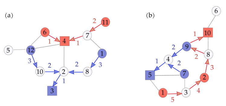
Some examples of feasible assignments of variables for both branching and flat models are shown in figures 1 and 2. On the left (figure 1 (a)) we see one instance of the V-DStP represented through the branching formalism and containing two sub-graphs, the “red” having root “4” and the “blue” rooted at node “3”; on the right (figure 1 (b)) two “red” and “blue” edge-disjoint Steiner trees, rooted at “10” and “5” respectively. Roots are represented as square nodes in contrast to circle colored nodes that are terminals. Edges employed in the solutions are figured as arrows whose labels denote the value of the (positive) depth component while the color mirrors the communication component. In agreement with our branching representation we see that depth components increase as we cover the solution from the root to the leaves for both problems. In the figure on the left, nodes of the vertex-disjoint trees are members either of the “red” or the “blue” trees but such constraint is relaxed in the figure 1 (b) for E-DStP. In fact, we allow node “9” to be a terminal of communication “blue” and a Steiner node of the “red” tree as two incident edges, $(10,9)$ and $(9,8)$, belong to the “red” solution.

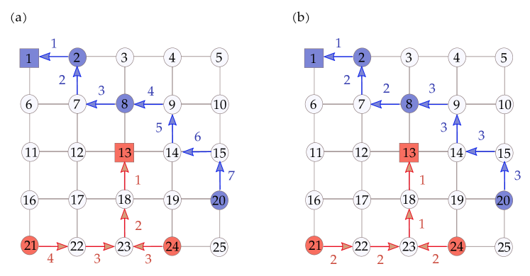
To underline the differences between the branching and the flat formalism, we picture in figure 2 (a) and (b) the same solution to the V-DStP on a grid graph using both models. According to the branching formalism, we see in figure 2 (a) that we need a minimum depth of $D=7$ to allow all terminals of the ”blue” communication to reach the root node “1” . Notice that since the tree is actually a chain of nodes, the same solution can be represented in the flat formalism using $D=3$ as shown in figure 2 (b). In fact, only each time we reach a terminal node the depth variable increases of one unit. Depth variables must increase in another condition, precisely when we reach a branching point: this is exactly what happens in the neighborhood of node “23” of the “red” solution in figure 2 (b).

Figure 1: Figures (a) and (b) show a feasible assignment of the variables for the V-DStP (left) and the E-DStP (right) using the branching model.

Figure 2: Figures (a) and (b) picture the same solution to a V-DStP using the branching formalism (figure (a)) and the flat representation (figure (b))

IV Boltzmann distribution and marginals

The formalism introduced above allows us to map each solution of the packing of Steiner trees to a certain assignment of variables $\boldsymbol{d}=\left\{d_{ij}:\left(i,j\right)\in E\right\}$ and $\boldsymbol{\mu}=\left\{\mu_{ij}:\left(i,j\right)\in E\right\}$ of the associated factor graph. The cost function in (1) can be then expressed in terms of the new variables as

$$H\left(\boldsymbol{d},\boldsymbol{\mu}\right)=\sum_{\mu=1}^{M}\left[\sum_{i\in V}c_{i}^{\mu}\prod_{k\in\partial i}\left(1-\delta_{\mu_{ki},\mu}\right)+\sum_{\begin{subarray}{c}d_{ij}>0:\\ \mu_{ij}=\mu\end{subarray}}w_{ij}\right]$$ (10)

where, for sake of simplicity, we consider the “homogeneous” case $w_{ij}^{\mu}=w_{ij},$ and $\psi_{i}$ can be either equal to $\psi_{i}^{V}$ or $\psi_{i}^{E}$.

The Boltzmann-Gibbs distribution associated with the energy $H\left(\boldsymbol{d},\boldsymbol{\mu}\right)$ is given by

$$P_{\beta}\left(\boldsymbol{d},\boldsymbol{\mu}\right)=\frac{\prod_{i}\psi_{i}\left(\boldsymbol{d}_{i},\boldsymbol{\mu}_{i}\right)e^{-\beta H\left(\boldsymbol{d},\boldsymbol{\mu}\right)}}{Z_{\beta}}$$ (11)

in which $\beta$ is a positive parameter, called the “inverse temperature” as in the statistical mechanics framework, and the normalization constant

$$Z_{\beta}=\sum_{\boldsymbol{d},\boldsymbol{\mu}}\prod_{i}\psi_{i}\left(\boldsymbol{d}_{i},\boldsymbol{\mu}_{i}\right)e^{-\beta H\left(\boldsymbol{d},\boldsymbol{\mu}\right)}$$

is the partition function. Configurations of the variables that do not satisfy the topological constraints will have zero probability measure, whereas all other configurations will be weighted according to the sum of weights of used edges and of the penalties of non-employed nodes. In the limit $\beta\rightarrow+\infty$ the distribution will be concentrated in the configuration that minimizes $H\left(\boldsymbol{d},\boldsymbol{\mu}\right)$ (the ground state of the system) that are exactly the solutions of the optimization problems. As a consequence also the marginal probability densities, for $\beta\rightarrow+\infty$, associated with each edge

$$P_{ij}^{\beta\rightarrow+\infty}\left(d_{ij},\mu_{ij}\right)=\sum_{\bar{\boldsymbol{d}},\bar{\boldsymbol{\mu}}}P_{\beta\rightarrow+\infty}\left(\boldsymbol{d},\boldsymbol{\mu}\right)\delta_{d_{ij},\bar{d}_{ij}}\delta_{\mu_{ij},\bar{\mu}_{ij}}\quad\forall\,\left(i,j\right)\in E$$ (12)

will be concentrated and therefore it suffices to estimate them to gain knowledge about the optimal configuration. Thus our assignment of the variables will be given by

$$\left(d_{ij}^{*},\mu_{ij}^{*}\right)=\arg\max_{\left(d_{ij},\mu_{ij}\right)}P_{ij}^{\beta\rightarrow+\infty}\left(d_{ij},\mu_{ij}\right)\quad\forall\,\left(i,j\right)\in E$$ (13)

Unfortunately the computation of (12) is impractical as it would require the calculation of a sum of an exponential number of terms. We seek to estimate these marginals via the cavity method approach. We report here a standard formulation of the cavity equations and we refer the interested reader to (mezard_information_2009, ) for the detailed derivation. At finite $\beta$ the BP equations on our factor graph are:

$$\begin{cases}m_{ij}\left(d_{ij},\mu_{ij}\right)&=\frac{1}{Z_{ij}}\sum_{\begin{subarray}{c}\left\{d_{ki},\mu_{ki}\right\}:\\ k\in\partial i\setminus j\end{subarray}}\psi_{i}\left(\boldsymbol{d}_{i},\boldsymbol{\mu}_{i}\right)e^{-\beta\sum_{\mu}c_{i}^{\mu}\prod_{k\in\partial i}\left(1-\delta_{\mu_{ki},\mu}\right)}\prod_{k\in\partial i\setminus j}n_{ki}\left(d_{ki},\mu_{ki}\right)\\ \\ n_{ki}\left(d_{ki},\mu_{ki}\right)&=e^{-\beta w_{ki}\mathbb{I}\left[d_{ki}>0\right]}m_{ki}\left(d_{ki},\mu_{ki}\right)\end{cases}$$ (14)

where

$$Z_{ij}=\sum_{\{d_{ij},\mu_{ij}\}}m_{ij}\left(d_{ij},\mu_{ij}\right)$$

is the normalization constant or “partial” partition function. The functions $m_{ij}$ are called cavity marginals or “messages”, suggesting that some information is flowing on edge $\left(i,j\right)$ within the factor graph from node $i$ to node $j$. In fact, the values of the messages $m_{ij}$ are in some sense proportional to the probability of a particular assignment $\left(d_{ij},\mu_{ij}\right)$ for edge $\left(i,j\right)$ if the node $j$ were temporarily erased from the graph.

The system of equations in (14) can be seen as fixed point equations that can be solved iteratively. Starting from a set of initial cavity marginals at time $t=0$, we iterate the right-hand-side of (14) until numerical convergence to a fixed point is reached. At convergence we calculate an approximation to marginals in (12) via the cavity fields defined as

$$M_{ij}\left(d_{ij},\mu_{ij}\right)\propto n_{ij}\left(d_{ij},\mu_{ij}\right)n_{ji}\left(-d_{ij},\mu_{ij}\right)$$ (15)

where the proportional sign denotes that a normalization constant is missing.

Cavity equations for optimization problems can be easily obtained by substituting the $m_{ij}$ and $M_{ij}$ with the variables $h_{ij}\left(d_{ij},\mu_{ij}\right)=\lim_{\beta\rightarrow\infty}\frac{1}{\beta}\log n\left(d_{ij},\mu_{ij}\right)$ and $H_{ij}\left(d_{ij},\mu_{ij}\right)=\lim_{\beta\rightarrow\infty}\frac{1}{\beta}\log M_{ij}\left(d_{ij},\mu_{ij}\right)$ into (14) and (15) that play the role of cavity marginals and fields in the zero-temperature limit; the resulting closed set of equations is known as the Max-Sum algorithm. At convergence we can extract our optimal assignment of variables by the computation of the decisional variables

$$\left(d_{ij}^{*},\mu_{ij}^{*}\right) = \arg\max_{\left(d_{ij},\mu_{ij}\right)}H_{ij}\left(d_{ij},\mu_{ij}\right)$$ (16)

$$H_{ij}\left(d_{ij},\mu_{ij}\right) = h_{ij}\left(d_{ij},\mu_{ij}\right)+h_{ji}\left(-d_{ij},\mu_{ij}\right)-C^{\prime}$$ (17)

where $C^{\prime}$ is an additive constant that guarantees that normalization condition in the zero-temperature limit, i.e. $\max_{\left(d_{ij},\mu_{ij}\right)}H_{ij}\left(d_{ij},\mu_{ij}\right)=0$, is satisfied. In practice, converge is reached when the decisional variables computed as in (16) do not change after a predefined number of successive iterations (often $10-30$). Notice that taking the $\beta\rightarrow+\infty$ limit of the message-passing equations at finite $\beta$ is not equivalent to the zero-temperature limit of the Boltzmann distribution in (11).

In the following section we will show how to derive equations for the cavity marginals and cavity fields, for finite $\beta$ and in the limit $\beta\rightarrow+\infty$, depending on we are dealing with the V-DStP or the E-DStP problem.

V The cavity equations

V.1 Vertex-disjoint Steiner trees Problem

To derive the Belief Propagation equations for the V-DStP problem suffices to impose $\psi_{i}\left(\boldsymbol{d}_{i},\boldsymbol{\mu}_{i}\right)=\psi_{i}^{V}\left(\boldsymbol{d}_{i},\boldsymbol{\mu}_{i}\right)$ in (14). By a change of variables, we will determine a Max-Sum algorithm for this variant.

Equations for messages can be easily obtained by using the properties of Kronecker delta functions in $\psi_{i}^{V}\left(\boldsymbol{d}_{i},\boldsymbol{\mu}_{i}\right)$; the explicit derivation in reported in appendix A. We can differentiate three cases depending on we are updating messages $n_{ij}$ for positive, negative or null depth $d_{ij}$:

$$\begin{cases}m_{ij}\left(d,\mu\right)=m_{+}^{b}\left(d,\mu\right)+m^{f}\left(d,\mu\right)&\quad\forall d>0,\mu\neq 0\\ m_{ij}\left(d,\mu\right)=m_{-}^{b}\left(d,\mu\right)+m^{f}\left(d,\mu\right)&\quad\forall d<0,\mu\neq 0\\ m_{ij}\left(0,0\right)=e^{-\beta\sum_{\mu}c_{i}^{\mu}}\prod_{k\in\partial i\backslash j}n_{ki}\left(0,0\right)+m_{0}^{b}+m_{0}^{f}\end{cases}$$ (18)

where $m_{+}^{b}\left(d,\mu\right),\,m_{-}^{b}\left(d,\mu\right),$ $m^{f}\left(d,\mu\right),$ and $m_{0}^{b},\,m_{0}^{f}$ are defined as

$$m_{+}^{b}\left(d,\mu\right) = \prod_{k\in\partial i\backslash j}\left[n_{ki}\left(d+1,\mu\right)+n_{ki}(0,0)\right]$$

$$m^{f}\left(d,\mu\right) = \delta_{c_{i}^{\mu},0}\sum_{k\in\partial i\backslash j}n_{ki}\left(d,\mu\right)\prod_{l\in\partial i\backslash\left\{j,k\right\}}n_{li}\left(0,0\right)$$

$$m_{-}^{b}\left(d,\mu\right) = \sum_{k\in\partial i\backslash j}n_{ki}\left(d+1,\mu\right)\prod_{l\in\partial i\backslash\{j,k\}}\left[n_{li}\left(d,\mu\right)+n_{li}(0,0)\right]$$

$$m_{0}^{b} = \sum_{\mu\neq 0}\sum_{d<0}m_{-}^{b}\left(d,\mu\right)$$

$$m_{0}^{f} = \sum_{\mu\neq 0}\sum_{d<0}\sum_{k\in\partial i\backslash j}n_{ki}\left(d,\mu\right)\sum_{l\in\partial i\backslash\left\{j,k\right\}}n_{li}\left(-d,\mu\right)\prod_{m\in\partial i\backslash\left\{k,l,j\right\}}n_{mi}\left(0,0\right)$$

Replacing $h_{ij}(d_{ij},\mu_{ij})=\lim_{\beta\rightarrow+\infty}n_{ij}\left(d_{ij},\mu_{ij}\right)$ in (18) we obtain the Max-Sum equations:

$$\begin{cases}h_{ij}\left(d,\mu\right)=\max\left\{h_{+}^{b}\left(d,\mu\right),h_{+}^{f}\left(d,\mu\right)\right\}&\quad\forall d>0,\mu\neq 0\\ h_{ij}\left(d,\mu\right)=\max\left\{h_{-}^{b}\left(d,\mu\right),h_{-}^{f}\left(d,\mu\right)\right\}&\quad\forall d<0,\mu\neq 0\\ h_{ij}\left(0,0\right)=\max\left\{-\sum_{\mu}c_{i}^{\mu}+\sum_{k\in\partial i\backslash j}h_{ki}\left(0,0\right),\;h_{0}^{b},\,\,h_{0}^{f}\right\}\end{cases}$$ (19)

for

$$h_{+}^{b}\left(d,\mu\right) = -w_{ij}+\sum_{k\in\partial i\backslash j}\max\left\{h_{ki}\left(d+1,\mu\right),h_{ki}\left(0,0\right)\right\}$$

$$h_{+}^{f}\left(d,\mu\right) = -w_{ij}+\log\delta_{c_{i}^{\mu},0}+\max_{k\in\partial i\backslash j}\left\{h_{ki}\left(d,\mu\right)+\sum_{l\in\partial i\backslash j}h_{li}\left(0,0\right)\right\}$$

$$h_{-}^{b}\left(d,\mu\right) = \max_{k\in\partial i\backslash j}\left[h_{ki}\left(d+1,\mu\right)-w_{ik}+\sum_{l\in\partial i\backslash\{j,k\}}\max\left\{h_{li}\left(d,\mu\right),h_{li}\left(0,0\right)\right\}\right]$$

$$h_{-}^{f}\left(d,\mu\right) = \log\delta_{c_{i}^{\mu},0}+\max_{k\in\partial i\backslash j}\left\{h_{ki}\left(d,\mu\right)-w_{ik}+\sum_{l\in\partial i\backslash j}h_{li}\left(0,0\right)\right\}$$

$$h_{0}^{b} = \max_{\mu\neq 0}\max_{d<0}h_{-}^{b}\left(d,\mu\right)$$

$$h_{0}^{f} = \max_{\mu\neq 0}\max_{d<0}\left[\max_{\begin{subarray}{c}k\in\partial i\setminus j\,,\\ l\in\partial i\backslash\{j,k\}\end{subarray}}h_{ki}\left(d,\mu\right)-w_{ik}+h_{li}\left(-d,\mu\right)+\sum_{m\in\partial i\backslash\left\{j,k,l\right\}}h_{mi}\left(0,0\right)\right]$$

V.2 Edge-disjoint Steiner trees problem

As for the V-DStP, the Belief Propagation equations for the E-DStP can be computed imposing $\psi_{i}\left(\boldsymbol{d}_{i},\boldsymbol{\mu}_{i}\right)=\psi_{i}^{E}\left(\boldsymbol{d}_{i},\boldsymbol{\mu}_{i}\right)$ into (14):

$$m_{ij}\left(d_{ij},\mu_{ij}\right)\propto\sum_{\begin{subarray}{c}\left\{d_{ki},\mu_{ki}\right\}:\\ k\in\partial i\setminus j\end{subarray}}\psi_{i}^{E}\left(\boldsymbol{d}_{i},\boldsymbol{\mu}_{i}\right)e^{-\beta\sum_{\mu}c_{i}^{\mu}\prod_{k\in\partial i}\left(1-\delta_{\mu_{ki},\mu}\right)}\prod_{k\in\partial i\setminus j}n_{ki}\left(d_{ki},\mu_{ki}\right)$$ (20)

Instead of considering the cavity messages as in V.1, to compute (20) we will first define a partial partition function

$$Z_{i}=\sum_{\boldsymbol{d}_{i},\boldsymbol{\mu}_{i}}\psi_{i}^{E}\left(\boldsymbol{d}_{i},\boldsymbol{\mu}_{i}\right)e^{-\beta\sum_{\mu}c_{i}^{\mu}\prod_{k\in\partial i}\left(1-\delta_{\mu_{ki},\mu}\right)}\prod_{k\in\partial i}n_{ki}\left(d_{ki},\mu_{ki}\right)$$ (21)

and then calculate the set of messages $m_{ij}\left(d,\mu\right)$ (for all possible values of $d$ and $\mu$) from $i$ to $j$ through (21) by temporarily setting the message that $i$ received from $j$ as $n_{ji}\left(d_{ji},\mu_{ji}\right)=\delta_{-d,d_{ji}}\delta_{\mu,\mu_{ji}}$. In fact, here $m_{ij}$ has a unique non-zero value in the state that satisfies the anti-symmetric property, namely $d_{ij}=d$, $\mu_{ij}=\mu$; under this condition $Z_{i}=m_{ij}\left(d_{ij},\mu_{ij}\right)$ up to a normalization constant. Due to the explicit expression of $\psi_{i}^{E}$ message-passing equations become intractable and, therefore, the update step of the algorithm cannot be efficiently implemented. In the following subsections we overcome this issue by proposing two different approaches for the computation of (21) where we make use of two different sets of auxiliary variables. The first formalism relies on “binary occupation” variables that denote, for each node of the factor graph, if edges incident on it are used or not by any communication; as we will see the associated computation scales exponentially in the degree of the nodes. The second one consists in a mapping between the E-DStP update equation and a weighted matching problem over bipartite graphs, that, in the $\beta\rightarrow+\infty$, becomes a weighted maximum matching problem which can be solved efficiently. This implementation scales exponentially with respect to $M$ but it may be more efficient for vertices with large degrees with respect to the first algorithm.

V.2.1 Neighbors occupation formalism

Suppose of associating with each vertex $i$ a vector $\boldsymbol{x}=\left\{0,1\right\}{}^{|\partial i|}$ that denotes if edges incident on $i$ are employed or unemployed within the solution. A feasible assignment of these auxiliary variables is guaranteed if, for every link $\left(i,k\right)\in E$ incident on $i$, we impose $x_{k}=1$ if the edge belongs to a tree (i.e. $d_{ki}\neq 0$ and consequently $\mu_{ki}\neq 0$) or $x_{k}=0$ otherwise (for $\mu_{ki}=0,\,d_{ki}=0$). Variables $\left(\boldsymbol{d}_{i},\boldsymbol{\mu}_{i}\right)$ must locally satisfy the following identity $\prod_{k\in\partial i}\mathbb{I}\left[x_{k}=1-\delta_{d_{ki},0}\right]=1$ for every node $i\in V$. If we insert this expression in (21) and we sum over all possible assignments of $\boldsymbol{x}$ variables we obtain

$$Z_{i} = \sum_{\boldsymbol{d}_{i},\boldsymbol{\mu}_{i}}\psi_{i}^{E}\left(\boldsymbol{d}_{i},\boldsymbol{\mu}_{i}\right)e^{-\beta\sum_{\mu}c_{i}^{\mu}\prod_{k\in\partial i}\left(1-\delta_{\mu_{ki},\mu}\right)}\sum_{\boldsymbol{x}}\prod_{j\in\partial i}\mathbb{I}\left[x_{j}=1-\delta_{d_{ji},0}\right]n_{ji}\left(d_{ji},\mu_{ji}\right)$$ (22)

$$= \sum_{\boldsymbol{x}}Z_{\mathbf{x}}^{M}$$ (23)

where $Z_{\boldsymbol{x}}^{M}$ is defined by computing the following expression for $q=M$

$$Z_{\boldsymbol{x}}^{q}\equiv\sum_{\begin{subarray}{c}\boldsymbol{d}_{i},\boldsymbol{\mu}_{i}\\ \mu_{ki}\leq q\end{subarray}}\psi_{i}^{E}\left(\boldsymbol{d}_{i},\boldsymbol{\mu}_{i}\right)e^{-\beta\sum_{\mu}c_{i}^{\mu}\prod_{k\in\partial i}\left(1-\delta_{\mu_{ki},\mu}\right)}\prod_{k\in\partial i}\mathbb{I}\left[x_{k}=1-\delta_{d_{ki},0}\right]n_{ki}\left(d_{ki},\mu_{ki}\right)$$ (24)

The computation of $Z_{\boldsymbol{x}}^{q}$ is then performed using the following recursion (the equivalence of (25) to (24) is proven in appendix B)

$$Z_{\boldsymbol{x}}^{q} = \sum_{\boldsymbol{y\leq\boldsymbol{x}}}\left(g_{\boldsymbol{y}}^{0}+g_{\boldsymbol{y}}^{b}+g_{\boldsymbol{y}}^{f}\right)Z_{\boldsymbol{y}}^{q-1}$$ (25)

$$Z_{\boldsymbol{x}}^{0} = e^{-\beta\sum_{\mu}c_{i}^{\mu}}\prod_{j\in\partial i}\delta_{x_{j},0}n_{ji}\left(0,0\right)$$ (26)

where the auxiliary functions $g_{\boldsymbol{y}}^{0},\,g_{\boldsymbol{y}}^{b},\,g_{\boldsymbol{y}}^{f}$ are defined as

$$g_{\boldsymbol{y}}^{0} = e^{-\beta c_{i}^{q}}\prod_{\begin{subarray}{c}k\in\partial i\\ y_{k}=0\\ x_{k}=1\end{subarray}}n_{ki}\left(0,0\right)$$

$$g_{\boldsymbol{y}}^{b} = \sum_{d>0}\sum_{\begin{subarray}{c}j\in\partial i\\ y_{j}=0\\ x_{j}=1\end{subarray}}n_{ji}\left(-d,q\right)\prod_{\begin{subarray}{c}k\in\partial i\setminus j\\ y_{k}=0\\ x_{k}=1\end{subarray}}\left[n_{ki}\left(d+1,q\right)+n_{ki}\left(0,0\right)\right]$$

$$g_{\boldsymbol{y}}^{f} = \delta_{c_{i}^{q},0}\sum_{d>0}\sum_{\begin{subarray}{c}j\in\partial i\\ y_{j}=0\\ x_{j}=1\end{subarray}}n_{ji}\left(-d,q\right)\sum_{\begin{subarray}{c}k\in\partial i\backslash j\\ y_{k}=0\\ x_{k}=1\end{subarray}}n_{ki}\left(d,q\right)\prod_{\begin{subarray}{c}l\in\partial i\setminus\left\{j,k\right\}\\ y_{l}=0\\ x_{l}=1\end{subarray}}n_{li}\left(0,0\right)$$

and the trace over $\boldsymbol{y}\leq\boldsymbol{x}$ denotes all possible vectors $\boldsymbol{y}=\left\{0,1\right\}{}^{|\partial i|}$ satisfying

$$y_{k}=\begin{cases}y_{k}\leq x_{k}&\mathrm{if}\,\mu_{ki}\neq q\\ 0&\mathrm{if}\,\mu_{ki}=q\end{cases}$$ (27)

Within the Max-Sum formalism,we can equivalently define a partial free entropy $F_{i}=\lim_{\beta\rightarrow+\infty}\frac{1}{\beta}\log Z_{i}$ and express it as function of Max-Sum messages $h_{ij}\left(d_{ij},\mu_{ij}\right)=\lim_{\beta\rightarrow+\infty}\frac{1}{\beta}\log n_{ij}\left(d_{ij},\mu_{ij}\right)$ as

$$F_{i}=\max_{\begin{subarray}{c}\boldsymbol{d}_{i},\boldsymbol{\mu}_{i}\\ \psi_{i}^{E}\left(\boldsymbol{d}_{i},\boldsymbol{\mu}_{i}\right)=1\end{subarray}}\max_{\boldsymbol{x}}\left[\sum_{k\in\partial i}\log\mathbb{I}\left[x_{k}=1-\delta_{d_{ki},0}\right]+h_{ki}\left(d_{ki},\mu_{ki}\right)-\sum_{\mu}c_{i}^{\mu}\prod_{k\in\partial i}\left(1-\delta_{\mu_{ki},\mu}\right)\right]$$ (28)

where the function $\sum_{k\in\partial i}\log\mathbb{I}\left[x_{k}=1-\delta_{d_{ki},0}\right]$ takes value zero if variables satisfy the constraints or minus infinity otherwise. As in the BP formulation, we rewrite it as

$$F_{i}=\max_{\boldsymbol{x}}F_{\boldsymbol{x}}^{M}$$ (29)

with

$$F_{\boldsymbol{x}}^{M}=\max_{\begin{subarray}{c}\boldsymbol{d}_{i},\boldsymbol{\mu}_{i}\\ \psi_{i}^{E}\left(\boldsymbol{d}_{i},\boldsymbol{\mu}_{i}\right)=1\end{subarray}}\sum_{k\in\partial i}\left[\log\mathbb{I}\left[x_{k}=1-\delta_{d_{ki},0}\right]+h_{ki}\left(d_{ki},\mu_{ki}\right)-\sum_{\mu}c_{i}^{\mu}\prod_{k\in\partial i}\left(1-\delta_{\mu_{ki},\mu}\right)\right]$$

The computation can be performed recursively from

$$F_{\boldsymbol{x}}^{q} =\max_{\boldsymbol{y\leq\boldsymbol{x}}}\left\{F_{\boldsymbol{y}}^{q-1}+\max\left\{h_{0},\,h_{b},\,h_{f}\right\}\right\}$$ (30)

$$F_{\mathbf{x}}^{0} =-\sum_{\mu}c_{i}^{\mu}+\log\mathbb{I}\left[\boldsymbol{x}=\boldsymbol{0}\right]+\sum_{k\in\partial i}h_{ki}\left(0,0\right)$$ (31)

where

$$h_{0} =\sum_{\begin{subarray}{c}k\in\partial i\\ y_{k}=0\\ x_{k}=1\end{subarray}}h_{ki}\left(0,0\right)-c_{i}^{q}$$ (32)

$$h_{b} =\max_{d>0}\max_{\begin{subarray}{c}k\in\partial i\\ y_{k}=0\\ x_{k}=1\end{subarray}}\left[h_{ki}\left(-d,q\right)+\sum_{\begin{subarray}{c}l\in\partial i\setminus k\\ y_{l}=0\\ x_{l}=1\end{subarray}}\max\left[h_{li}\left(d+1,q\right),h_{li}\left(0,0\right)\right]\right]$$ (33)

$$h_{f} =\log\delta_{c_{i}^{q},0}+\max_{d>0}\left[\max_{\begin{subarray}{c}k\in\partial i,\,l\in\partial i,\,k\neq l\\ y_{k}=0,\,y_{l}=0\\ x_{k}=1\,x_{l}=1\end{subarray}}h_{ki}\left(-d,q\right)+h_{li}\left(d,q\right)+\sum_{\begin{subarray}{c}m\in\partial i\backslash\{k,l\}\\ y_{m}=0\\ x_{m}=1\end{subarray}}h_{mi}\left(0,0\right)\right]$$ (34)

V.2.2 Mapping into a matching problem

We will develop an alternative method for the computation of the messages of BP and MS update equations, that can lead to an exponential speedup in some cases. Let us introduce an auxiliary vector $\boldsymbol{s}\in\left\{0,1,\dots,D\right\}^{M}$ associated with each vertex of the graph. Components $s_{\mu}$ take value in the set of the possible positive depths $\left\{1,\ldots,D\right\}$ if this node is member of communication $\mu$ or $0$ otherwise. For a node $i$ that is not a root but a member of the communication $\mu$, there exists exactly one neighbor $k$ such that $d_{ik}>0$, $d_{ki}=-s_{\mu_{ki}}\,\mu_{ki}=\mu$ and for the remaining ones, $d_{li}\delta_{\mu_{li},\mu}=s_{\mu_{ki}}+1$ or $d_{li}\delta_{\mu_{li},\mu}=0$, $l\in\partial i\backslash k$. The compatibility function for E-DStP can be expressed as a function of the new variables as

$$\psi_{i}^{E}\left(\boldsymbol{d}_{i},\boldsymbol{\mu}_{i}\right) = \prod_{\mu=1}^{M}\left[\sum_{s_{\mu}>0}\sum_{k\in\partial i}\delta_{\tilde{d}_{ki},-s_{\mu}}\prod_{l\in\partial i\setminus k}\left(\delta_{\tilde{d}_{li},s_{\mu}+1}+\delta_{\tilde{d}_{li},0}\right)+\prod_{k\in\partial i}\delta_{\tilde{d}_{ki},0}\right]$$ (35)

$$= \sum_{\mathbf{s}}\left\{\prod_{\mu=1}^{M}\left(1-\delta_{s_{\mu},0}\right)\sum_{k\in\partial i}\left[\delta_{\tilde{d}_{ki},-s_{\mu}}\prod_{l\in\partial i\setminus k}\left(\delta_{\tilde{d}_{li},s_{\mu}+1}+\delta_{\tilde{d}_{li},0}\right)\right]+\prod_{\mu=1}^{M}\delta_{s_{\mu},0}\prod_{k\in\partial i}\delta_{\tilde{d}_{ki},0}\right\}$$ (36)

As introduced in the neighbors occupation formalism, we will compute the update equations from $Z_{i}$, that, within this formalism can be written as

$$Z_{i} = \sum_{\boldsymbol{s}}R_{\boldsymbol{s}}Z_{\boldsymbol{s}}$$ (37)

where

$$R_{\boldsymbol{s}} = \prod_{k\in\partial i}\left[\sum_{\nu}n_{ki}\left(s_{\nu}+1,\nu\right)+n_{ki}\left(0,0\right)\right]$$ (38)

$$Z_{\boldsymbol{s}} = \sum_{\boldsymbol{t}}\prod_{\mu}e^{-\beta c_{i}^{\mu}\mathbb{I}\left[s_{\mu}=0\right]}\mathbb{I}\left[\sum_{k\in\partial i}t_{k\mu}=1-\delta_{s_{\mu},0}\right]\prod_{k\in\partial i}\mathbb{I}\left[\sum_{\mu}t_{k\mu}\leq 1\right]\prod_{k\in\partial i}\left[\frac{n_{ki}\left(-s_{\mu},\mu\right)}{\sum_{\nu}n_{ki}\left(s_{\nu}+1,\nu\right)+n_{ki}\left(0,0\right)}\right]^{t_{k\mu}}$$ (39)

The components $t_{k\mu}$ of vectors $\boldsymbol{t}$ take value 1 if $k\in\partial i$ participate to sub-graph $\mu$ at distance $s_{\mu}>0$ from the root or 0 otherwise. The derivation of (37) is reported in appendix C. The term $Z_{\boldsymbol{s}}$ is the partition function of a matching problem on the complete bipartite graph $G=\left(V=A\cup B,E=A\times B\right)$ with $A=\partial i$ and $B=\left\{\mu:s_{\mu}>0\right\}$, and the energy of a matching is

$$\epsilon\left(\boldsymbol{t}\right)=\sum_{k\mu}t_{k\mu}\log\frac{n_{ki}\left(-s_{\mu},\mu\right)}{\sum_{\nu}n_{ki}\left(s_{\nu}+1,\mu\right)+n_{ki}\left(0,0\right)}-\beta c_{i}^{\mu}\mathbb{I}\left[s_{\mu}=0\right]$$

Notice that the partition function $Z_{\mathbf{s}}$ is computationally intractable as it corresponds to the calculation of a matrix permanent. In the $\beta\to\infty$ limit we can introduce the Max-Sum messages $h_{ki}\left(-s_{\mu},\mu\right)=\frac{1}{\beta}\log n_{ki}\left(-s_{\mu},\mu\right)$ and directly compute the free entropy $F_{i}=\frac{1}{\beta}\log Z_{i}$ that fortunately reduces to the evaluation of

$$F_{i} = \max_{\boldsymbol{s}}\left[\frac{1}{\beta}\left(\log R_{\boldsymbol{s}}+\log Z_{\boldsymbol{s}}\right)\right]$$ (40)

$$= \max_{\mathbf{s}}\left\{\sum_{k\in\partial i}\max\left[\max_{\mu}h_{ki}\left(s_{\mu}+1,\mu\right),\;h_{ki}\left(0,0\right)\right]+F_{\mathbf{s}}\right\}$$ (41)

The second term $F_{\boldsymbol{s}}=\frac{1}{\beta}\log Z_{\boldsymbol{s}}$ is the free entropy of the solution of a weighted maximum matching problem on a bipartite graph which can be performed in polynomial time (precisely, in $O\left(\left(M+\left|\partial i\right|\right)^{2}M\left|\partial i\right|\right))$. Indeed, for each assignment of the $\boldsymbol{s}$ we can define the weights $w_{k\mu}$ associated with each edge $(k,\mu)$ as

$$w_{k\mu}=\begin{cases}h_{ki}\left(-s_{\mu},\mu\right)-\max_{\nu}\max\left\{h_{ki}\left(s_{\nu}+1,\nu\right),h_{ki}\left(0,0\right)\right\}&\mbox{ if }s_{\mu}>0\\ -c_{i}^{\mu}&\mbox{ if }s_{\mu}=0\end{cases}$$ (42)

and solve

$$\begin{cases}F_{\boldsymbol{s}}=\max\sum_{\left(k,\mu\right)}w_{k\mu}t_{k\mu}&:\\ \sum_{k\in\partial i}t_{k\mu}\leq 1&\quad\forall\mu\\ \sum_{\mu}t_{k\mu}\leq 1&\quad\forall k\in\partial i\end{cases}$$ (43)

The system in (43) describes an integer linear problem for the resolution of a bipartite maximum weighted matching problem . Its relaxation to real variables $\boldsymbol{t}$can be efficiently solved and moreover the optimal solution is proven to be integer, that is for binary $\boldsymbol{t}$.

V.3 The parameter $D$

The branching formalism introduced in III relies on a parameter $D$ that denotes the maximum allowed distance between the root and the leaves of any tree. This parameter limits the depth of solution-trees and therefore the goodness of the results: a small value for $D$ may prevent the connection of some terminals but a large value of $D$ will slow down the algorithm affecting the converge. Thus the value of $D$ needs to be carefully designed to ensure good performances. Although there is not a clear technique able to predict the best setting, some heuristics have been proposed in recent works to determine a minimum feasible value of $D$ for the MStP and PCStP (biazzo_performance_2012, ). In this work, we adopt methods described in (braunstein_practical_2016, ) to find a minimum value of $D_{\mu}$ for each communication $\mu$ and we than set $D=\max_{\mu}D_{\mu}$.

It is clear that the computing cost of both V-DStP and E-DStP strongly depends on the value of $D$, more precisely linearly for the V-DStP and the binary occupation formalism and polynomially for the matching problem formulation for the E-DStP, and it could be still prohibit for graph with large diameter. Fortunately, the use of the flat formalism allows us to reduce the parameter $D$ to $D=\max_{\mu}\left|T_{\mu}\right|$ being $\left|T_{\mu}\right|$ the number of terminals of communication $\mu$. A proof of this property is reported in (braunstein_practical_2016, ) for the single tree problem.

VI Max-Sum for loopy graphs

The goodness of the approximation of the marginals is strictly related to the properties of the factor graph over which we run the Belief Propagation algorithm. BP is exact on tree graphs but nevertheless benefits from nice convergence properties even on general, loopy, graphs that are locally tree-like (weiss_optimality_2001, ). In the framework of the PCStP and multiple trees variants, there are several instances of practical interest, such as square or cubic lattices (2D or 3D graphs) modelling VLSI circuits, where many very short loops exist and the assumption of negligible correlation among variables is not satisfied. In many of these cases MS fails to converge in most of the trials or it requires a prohibitive run-time (braunstein_practical_2016, ).

We employ here a reinforcement scheme (bayati_statistical_2008, ; biazzo_performance_2012, ) that is able to make the algorithm converge on a tunable amount of time with the drawback that the solution may be sub-optimal in terms of cost. From the viewpoint of the factor graph it adds an extra factor to edge-variables that acts as an external field oriented in the direction of the cavity fields of past iterations. It slightly modifies the original problem into an easier one where a feasible assignment of variables is more likely to occur. The strength of this perturbation increases linearly in time in a way that, after few iterations, first inaccurate predictions will be neglected but, after many iterations of MS, it let the algorithm converge to, hopefully, an assignments of variables satisfying all the constraints. We report in section VI.1 how to modify the Max-Sum equations for the V-DStP and E-DStP for including the reinforcement factor.

The reinforcement or bootstrapping procedure described in the following sub-section is generally sufficient to guarantee convergence on random networks. In practice, however, MS did not converge in some benchmark instances, even adopting the bootstrapping procedure. In (braunstein_practical_2016, ) we have shown how to complement the MS equations with heuristics to solve PCStP instances in an efficient and competitive way. At each iteration we perform a re-weight of node prizes and edge weights according to temporarily Max-Sum predictions and we then apply a heuristics to find a tree connecting all nodes of the modified graph. After a pruning procedure, we obtain a pruned minimum spanning tree which is surely a feasible candidate solution for the PCStP. The motivation is based on the fact that although Max-Sum often outputs inconsistent configurations while trying to reach the optimal assignment of variables, it still contains some valuable information. Heuristics have the responsibility of adjusting the assignments of the temporarily decisional variables guaranteeing a tree-structured solution for any iteration of the main algorithm. Furthermore heuristics results do not depend on the parameter $D$ of the model and they can provide solution-trees of any diameter. We show in section VI.2 how to generalize the combination of Max-Sum and heuristics in the case of multiple trees for the V-DStP and the E-DStP.

VI.1 Reinforcement

Within the bootstrap procedure and for each iteration $t$ of the algorithm,we compute the messages $h_{ij}^{t}$ and the cavity fields $H_{ij}^{t}$ as functions of the original messages $\bar{h}_{ij}^{t}$ as

$$h_{ij}^{t}\left(d_{ji},\mu_{ji}\right) \leftarrow\bar{h}_{ji}^{t}\left(d_{ij},\mu_{ji}\right)+\gamma_{t}H_{ji}^{t-1}\left(d_{ji},\mu_{ji}\right)$$ (44)

$$H_{ij}^{t}\left(d_{ij},\mu_{ij}\right) \propto\bar{h}_{ij}^{t}\left(d_{ij},\mu_{ij}\right)+\bar{h}_{ji}^{t}\left(-d_{ij},\mu_{ij}\right)+\gamma_{t}H_{ij}^{t-1}\left(d_{ij},\mu_{ij}\right)$$ (45)

The parameter $\gamma_{t}=t\gamma_{0}$ is linearly proportional to $\gamma_{0}$ which is the reinforcement factor that governs the strength of the bootstrap. It is usually very small, of the order of $10^{-5}$ not to deviate the dynamics towards the minimum of the energy and thus affect the goodness of the solution.

VI.2 Max-Sum based heuristics

At each iteration of the main algorithm we perform a re-weighting of the graph to favor MS temporarily predictions and we then apply two fast heuristics to find as many spanning trees as the number of communications that we want to pack. These trees will be carefully pruned in order to decrease the cost of the solution. In this work we design two different re-weighting schemes for two different heuristics and we refer the interested reader to the single-tree heuristics explained in (braunstein_practical_2016, ) for additional details. For each sub-graph $\mu$ we apply one of the two schemes as follows.

VI.2.1 Shortest Path Tree

For any MS iteration $t$ we compute the auxiliary weights of a sub-graph $\mu$ as

$$w_{ij}^{t}=\max_{d\neq 0}\left|H_{ij}^{t}\left(d,\mu\right)\right|$$ (46)

Notice that since the field $H_{ij}^{t}$ is normalized, there exists only one assignment of the variables such that $H_{ij}^{t}\left(d^{*},\mu\right)=0$ in correspondence of the most probable state $\left(d^{*},\mu^{*}\right)$; the field computed in all remaining states will be as negative as the probability of the corresponding edge to be not employed in the (temporary) MS solution. For this reason we allow edges in (46) to have zero weights if they are likely to be exploited within communication $\mu$ (they would have $d^{*}\neq 0$); differently, we penalize edges that, according to MS, must not be used (for which $d^{*}=0$) imposing strictly positive weights equal to the (minus) MS field computed at the most probable non-zero depth, which corresponds, in this case, to the second maximum of $\max_{d}\left|H_{ij}^{t}\left(d,\mu\right)\right|$.

We then compute the Shortest Paths Tree (SPT) of the modified graph and we prune the solution tree removing a leaf $i$ if it is not a terminal (for the MStP), and edges $\left(i,j\right)$ satisfying $w_{ij}>c_{i}^{\mu}$ (for the PCStP); we repeat this procedure until we do not find such leaves.

VI.2.2 Minimum Spanning Tree

In this scheme we assign auxiliary costs to nodes of the graph according to MS prediction. Let us consider the two auxiliary functions

$$\begin{cases}h_{i}\left(d,\mu\right)=\max_{k\in\partial i}\left\{h_{ik}^{t}(-d,\mu)+\sum_{l\in\partial i\setminus k}\max\left[h_{li}^{t}\left(d+1,\mu\right),h_{li}^{t}\left(0,\mu\right)\right]\right\}&\quad\mbox{ for }d>0\\ h_{i}\left(0,\mu\right)=\sum_{k\in\partial i}h_{ki}^{t}(0,\mu)-c_{i}^{\mu}\end{cases}$$ (47)

A node satisfying $\max_{d>0}h_{i}\left(d,\mu\right)<h_{i}\left(0,\mu\right)$ will be penalized assigning to edges incident on it a large cost $C$. We then apply the Minimum Spanning Tree (MST) algorithm to the modified graph and we prune the solution as in the case of the SPT.

Heuristics are applied to the graph for all the communications providing, for both E-DStP and V-DStP, a superposition of single-tree solutions. Notice that heuristics are sequentially applied, i.e. we consider one communication at the time, and depending on we are dealing with V-DStP or E-DStP, edges (and Steiner nodes for the V-DStP) selected in the first spanning trees cannot be further used by the successive applications. To overcome this problem, we add an erasing step before the application of each heuristics in which we delete edges (and eventually Steiner nodes) used by other communications. For V-DStP we only need to cut edges incident on terminals of other sub-graphs to satisfy nodes-disjoint constraints. Unfortunately such strong edge cutting procedure may lead to a graph with disconnected components or a graph in which the terminals that we aim at connecting may be isolated. In these scenarios we cannot find further trees able to span the modified graph and thus this heuristic approach fails. One way of preventing this problem is to randomize the order of the trees over which we apply the heuristics.

VII Numerical results

In this section we report the results for several experiments on synthetic networks and on benchmark, real-world, instances for the VLSI. In all the cases we will solve the V-DStP or the E-DStP where terminals have infinite prizes, i.e. the MStP variant, and a predefined root is selected for each sub-graph. The synthetic networks we chose are fully connected, regular or grid graphs, whose properties will allow us to underline the main features of the models and formalisms introduced in this work. In particular, by means of the fully connected graphs we will illustrate the improvements carried by Max-Sum against a “greedy” search of the solutions introduced in section VII.1 Furthermore, regular graphs allow us to verify the different scaling of the running time with respect to the degree of the graph of the two algorithms presented for the E-DStP. Motivated by their importance on technological applications, namely in the the design of VLSI, we also show some results on grid, both synthetic and real-word, graphs: here we will underline the improvements carried by the flat model. Generally, energies are averaged over several instances, meaning different realizations of the weighting of the edges and assignment of the terminals, of the same graph. To measure the energy gap of the solutions found by the two different procedures, for instance “x” and “y” algorithms, we measure the quantity $\frac{E_{x}-E_{y}}{E_{y}}$ assuming that $E_{x}$ and $E_{y}$ are the energies of the solutions found by algorithm “x” and “y” respectively. If the gap is positive (negative) the “x” (“y”) algorithm outperforms the other one.

We underline that, due to the intrinsic difficulty of the problem, there are very few (exact or approximate) results in literature and few algorithms to use for the comparison. In the case of VLSI circuits, we report the solution costs of a state-of-the art linear programming technique for the V-DStP published in (hoang_steiner_2012, ). This algorithm is not publicly available and thus it cannot be used for further comparisons.

VII.1 Greedy algorithm

The “greedy” procedure consists in solving, for each communication of the graph, the corresponding single-tree MStP by means of the MS algorithm combined with the bootstrap. To ensure that the superposition of these trees is a feasible candidate solution for the packing problem, we performed, as in the case of the heuristics described in section VI.2, a pre-processing of the graph before any application of the single-tree algorithm. In particular, whenever we try to propose a solution for the sub-graph $\mu$, we cut any terminal node, and all edges incident on it, of the communications that have not yet been considered, together with edges (and Steiner tree nodes for the V-DStP variant) of the communications that we have already connected. The “greedy” energy is given by the sum of energies of single-tree solutions.Notice that this “greedy” procedure is actually as hard as the packing problem, since even the MStP belongs to NP-hard class of problem; nevertheless this procedure will be useful to underline the benefits carried by the parallel (packing) search against the “greedy” and sequential one.

VII.2 Fully connected graphs

Here we report results for the V-DStP on fully connected graphs where we aim at packing $M=3$ trees. We compare our performances against the “greedy” procedure.

We deal with fully connected graphs because here the existence of a trivial solution of the packing problem, consisting in a chain of terminal nodes, is always guaranteed. We perform two different experiments: we first fix the size of the graphs (500 nodes) and we study how energies and gaps change for an increasing number of terminals nodes. Secondly, we fix the fraction of terminals per communication, more precisely for $\alpha=\frac{T_{\mu}}{N}=0.08,\,\mu\in\left\{1,2,3\right\}$ and we compare the performances as we increase the size of the graphs (from 100 to 700 nodes). We run both algorithms with fixed parameters $D=\{3,5,10\}$ and fixed reinforcement factor $\gamma_{0}=10^{-5}$.

VII.2.1 Uncorrelated edge weights

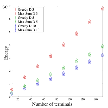
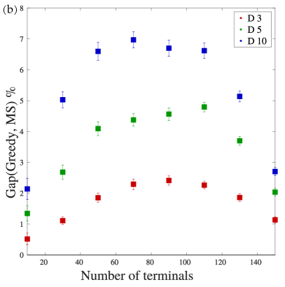
These experiments are performed on fully connected graphs where weights associated with edges are independently and uniformly distributed random variables in the interval $\left(0,1\right)$. In this scenario, energies obtained by the greedy procedure are always larger than the ones achieved by the parallel search, for all values of the number of terminals and for any value of the parameter $D$ used, as it is suggested by the plot of the gaps (right plot) in figure 3. Notice that the gaps are slightly greater than zero suggesting that solutions found by the two methods are very similar in terms of energy cost, as reported in the plot in figure 3, left panel.

Figure 3: Energy (a) and energy gap (b) of the solutions of Max Sum and Greedy algorithm as functions of the number of terminals. The test instances are fully connected graphs of 500 nodes with uncorrelated edge weights. Gaps reported in panel (b) are always positive suggesting that solutions found by the global search are cheaper in terms of cost than the greedy ones.

VII.2.2 Correlated edge weights

To underline the benefits carried by the optimized strategy, we run reinforced and greedy reinforced Max-Sum on complete graphs with correlated edge weights. With each node $i$ we assign a uniformly distributed random variable $x_{i}$ in the interval $\left(0,1\right)$ and for each edge $\left(i,j\right)$ we pick a variable $y_{ij}\in\left(0,1\right)$. Then an edge $\left(i,j\right)$ will be characterized by a weight $w_{ij}=x_{i}x_{j}y_{ij}$. Here we expect that the cheapest edges will be chosen by the “greedy” algorithm for the solution of the first trees and, as we proceed with the sequential search, the algorithm will become the more and more forced to use the remaining expensive edges. In fact, as shown in figure 4, the gaps notably increase of one order of magnitude for most of the number of terminals considered in these experiments.

Notice that energies encountered for $D=\left\{5,10\right\}$ are very close to one another suggesting that a further increasing of the parameter $D$, and thus of the solution space, will not lead to a significant improvement of the solutions.

Figure 4: Energy (a) and energy gap (b) for Max Sum results against Greedy results as functions of the number of terminals for correlated edge weighting. The energy gaps of panel (b) are positive and notably large.

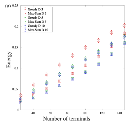
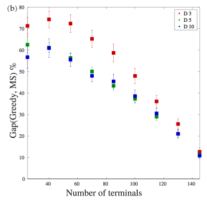
VII.2.3 Fixed fraction of terminals

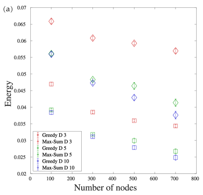
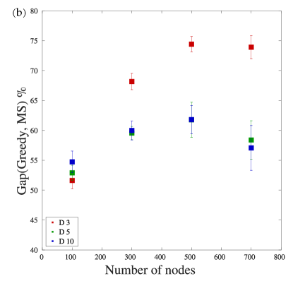
To study the performances in the asymptotic limit, namely for $N\rightarrow+\infty$ ,$T_{\mu}\rightarrow+\infty$ for each communication $\mu$ and constant $\alpha$, we attempted the solution of V-DStP on complete graphs having a fixed fraction of terminals $\alpha=0.08$ and for an increasing number of nodes $N$. Although non-rigorous, this procedure can suggest us the behavior of the energies and the energy gaps in the large $N$ limit. As reported in figure 5 panel (a), when the number of nodes reaches $N\in[500,\,700]$, the energy of both Max Sum and greedy solutions, for all values of $D$, seems to stabilize to a constant value. As a consequence, as plotted in figure 5 panel (b), also energy gaps fluctuates around a fixed value that seems to be different if one considers $D=3$ or $D=\left\{5,10\right\}$.

Figure 5: Energy (a) and energy gap (b) for Max Sum against Greedy results as functions of the number of nodes for a fixed fractions of terminals (per communication)$\alpha=0.08$.

VII.3 Regular graphs

In section V.2 we have seen how to deal with the update equations of BP and MS algorithms for the E-DStP with the help of two different auxiliary set of variables. Although the final expressions of the equations are very different, the energies obtained by both algorithms must be identical; the only differences rely on the computational cost that strongly depends on the properties of the graph, precisely on the degree of the nodes of the graph and on the number of communications. To underline these two features of the neighbors occupation formalism and matching problem mapping, that from now will be denoted as NeighOcc and Matching algorithms, we perform two different experiments on regular, fixed degree, graphs for different values of the degree and of the number of sub-graphs. For these simulations we have fixed the values of the parameter $D=10$ and the reinforcement factor $\gamma_{0}=10^{-4}$.

VII.3.1 Energy as a function of the degree

Similarly to the experiments in section VII.3.2, here we consider regular graphs of $N=50$ nodes containing $M=3$ sub-graphs for four possible degrees $d\in\left\{3,4,5,6\right\}$. The energies provided by NeighOcc and Matching and plotted in figure 6, panel (a), can be statistically considered the same, as for the fixed degree experiment shown before. Here the computational costs (panel (b) and (c) of figure 6) scales exponentially only for the NeighOcc (as it is remarked by the linear trend in the semi-log plot) while it scales polynomially for the Matching formalism as predicted by the analysis on the update equations in section V.2.

VII.3.2 Energy as a function of the number of communications

In this experiment we try to solve the E-DStP on two sets of regular graphs of $N=50$ nodes having fixed degree $4$, for an increasing number of trees. Each communication has the same number of terminals $T=3$. As shown in figure 6, panel (d), the energy costs of the solutions provided by NeighOcc and Matching algorithms are almost identical as we expected. At the same time, the computing time plotted in figure 6, panels (e) and (f), shows that the Matching procedure needs a time that scales exponentially, i.e. linearly in an log-scale plot, on the number of sub-graphs while it becomes polynomial for the NeighOcc algorithm.

Figure 6: In panel (a), energy of the solutions for the E-DStP on regular graphs of 3 communications as a function of the degree. In (b) and (c) running time of Matching and NeighOcc algorithms as a functions of degree. In panel (d): energy of the solutions for the E-DStP on regular graphs as a function of the number of packed trees. Panels (e) and (f): running time of the Matching and NeighOcc algorithms as a functions of the number of communications. In all plots energies of the solutions are almost the same, but the computing time dramatically differ as we are using the Matching formalism or the NeighOcc algorithm.

VII.4 Grid graphs

This section is devoted to the illustration of results of both V-DStP and E-DStP on 2D and 3D lattices. The first experiments are performed on synthetic 3D lattices of dimension $5\times 5\times 5$ containing $N=125$ nodes. Here we fix the number of communications $M\in\left\{2,3,4\right\}$ and we study how energies behave when the number of terminals $T$ per communication changes in the range $\left[3,\,6\right]$. For the V-DStP and the E-DStP (only in the NeighOcc formalism) we compare the results provided by the branching and flat models. While the parameter $D$ can be arbitrary large for the branching model, we keep the value $D=T$ for the flat one since, as discussed in section III.0.2, it is sufficient to explore all the solution space. In the second part of this section we comment the performances of the MS algorithm and of the MS-based heuristics presented in section VI.2 applied to several benchmark instances for the design problem of VLSI circuits.

VII.4.1 Branching and flat models for the V-DStP e E-DStP (neighbors occupation formalism)

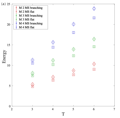
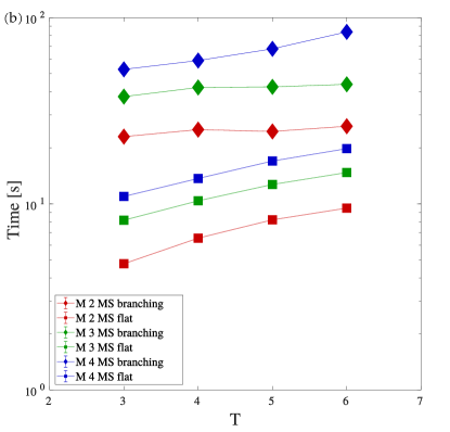
As shown in figure 7, left panel, the energies of the solutions found by the flat model for the V-DStP are always smaller than the energies found by the branching one. We underline that, as plotted in the right panel of figure 7, the flat version of MS equations has the advantage of converging in a running time that is always smaller than the one needed by the branching model. This is reasonable as the parameter $D$, which linearly influences the computation time of both algorithms, is often greater (on average $D=8$) for the branching model than the one fixed for the flat representation.

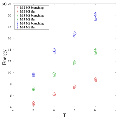
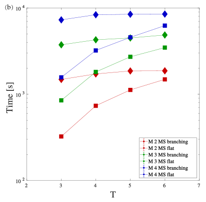
A different behavior is observed for the resolution of the E-DStP on grids using our two models. As remarked in figure 8, left panel, energies found by the flat and branching representations are comparable; here the depth used by the branching model, on average equal to $D=8\,\mathrm{and\,}D=9$ for $T\in\left[3,4\right]\,\mathrm{and\,T\in\left[5,6\right]}\,$ respectively, probably suffices to explore the same solution space considered by the flat formalism for smaller $D$. Still, the flat model is preferable as it requires a computing time that is smaller than the one needed by the branching model for all the cases we have considered.

Figure 7: Energy (a) and computational time (b) as a function of the number of terminals per communications for 3D grid graphs, V-DStP variant.

Figure 8: Energy (a) and computational time (b) as a function of the number of terminals per communications for 3D grid graphs, E-DStP variant.

VII.4.2 V-DStP for VLSI circuits

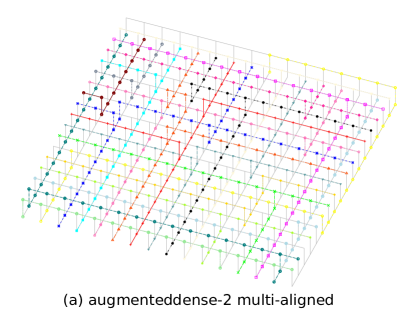
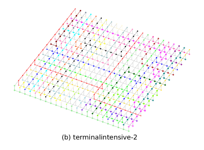
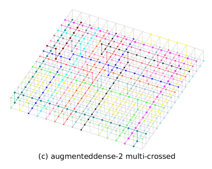
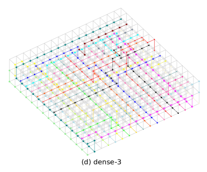
In this section we report several results for standard benchmark instances of circuit layout where we solve the V-DStP. Instances are 3D grid graphs modelling VLSI chips where we pack relatively many trees, usually 19 or 24, each of which typically contains few terminal nodes (3 or 4). Such grid graphs can be seen as multi-layers graphs where we allow two different kinds of connections. In the multi-crossed layers, each node is connected to all its possible neighbors in all directions: the resulting graphs are cubic lattices. The multi-aligned layers are similar to the multi-crossed ones but in each layer we allow only connections in one direction, either east-to-west or north-to-south (hoang_steiner_2012, ). For sake of simplicity, consider a cubic lattice in a three dimensional Cartesian coordinate system: depending on the value of the $z-$coordinate, the allowed connections will be present in directions parallel to the $x$ or to the $y$ axes. In table 1 we first report some information (type of the layers, size, number of sub-graphs and total number of terminals) concerning each instance and our results. We show the energies achieved by reinforced Max Sum along with the ones of the two heuristics described in section VI.2; in analogy with (braunstein_practical_2016, ), we label as “J” heuristics that performs a modified SPT and as “N” if instead we use the MST. Energies obtained using the flat model are labeled as “(f)” while if nothing is specified or “(b)” is used, we made use of the branching representation. Results are compared with respect to the ones obtained through state-of-the-art linear programming (LP) techniques (hoang_steiner_2012, ) which is able, for these particular instances, to find the optimal solutions. The sign “-” denotes that no solution has been found. As shown in table 1, the gaps between the best energies achieved by MS (in bold letters) and LP are always smaller than $4\%$ and in two cases, for the multi-aligned augmenteddense-2 and terminalintensive-2 instances, we reach the same performances of LP, obtaining the optimal solutions. We stress that these graphs are very loopy and far from being locally tree-like but nevertheless we achieve good performances thanks to the reinforcement procedure along with the introduction of the modified heuristics. Four examples of VLSI solutions are plotted in figure 9.

It is worth noting that the greedy procedure (repeated for several permutations of the order in which the trees were considered) fails after few sequential searches. The average number of packed trees $\left\langle M\right\rangle$ before the stop of the algorithm is reported in the last column of table 1. After these greedy steps there exists one communication for which the connection of all terminals is impossible: either the remaining graph, after the pruning described in section VII.1, is composed of disconnected components (one or more terminals are disconnected from the rest of the network) or a possible connection may violate the hard topological constraints.

	Type	Size	$M$	$T_{tot}$	Heur. “J”	Heur. “N”	Rein. Max Sum	LP (opt)	Gap (MS, LP) %	$\left\langle M\right\rangle$ Greedy
augmenteddense-2	Multi-aligned	16x18x2	19	59	504 (b) 506 (f)	507	508 (f) 504 (b)	504	0 %	14 (b) 2 (f)
augmenteddense-2	Multi-crossed	16x18x2	19	59	503	-	-	498	1.0 %	7 (b) 5 (f)
dense-3	Multi-crossed	15x17x3	19	59	487	488	485	464	4.0 %	11 (b) 7 (f)
difficult-2	Multi-aligned	23x15x2	24	66	535	538	538	526	1.7 %	15 (b) 6 (f)
difficult-2x	Multi-aligned	23x15x2	24	66	560	-	-	unknown		14 (b) 4 (f)
difficult-2y	Multi-aligned	23x15x2	24	66	4776	4829	4816	unknown		14 (b) 8 (f)
difficult-2z	Multi-aligned	23x15x2	24	66	1060	1063	1061	unknown		16 (b) 7 (f)
modifieddense-3	Multi-crossed	16x17x3	19	59	492	496	495	479	2.6 %	10 (b) 3 (f)
moredifficult-2	Multi-aligned	22x15x2	24	65	542	542	546	522	3.8 %	13 (b) 5(f)
pedabox-2	Multi-aligned	15x16x2	22	56	405	405	405	390	3.8 %	10 (b) 5 (f)
terminalintensive-2	Multi-aligned	23x16x2	24	77	596 (f) 599 (b)	617	620	596	0 %	13 (b) 5 (f)

Table 1: Results for circuit layout instances

Figure 9: Examples of solutions for the V-DStP on VLSI circuits for multi-aligned, (a) and (b) figures, and multi-crossed, (c) and (d) figures, layouts

VIII Summary of results

Using Max-Sum algorithm, we have explored through simulations some interesting theoretical questions in random graphs which we summarize here. Simulations (up to $N=700$, or around $2\times 10^{5}$ edges) suggest that for the Steiner Tree packing problem on complete graphs with uniform independent weights, the energy converges to a constant value if the fraction of terminal vertices is kept constant, in agreement with known results for single Steiner trees (angel_sharp_2012, ).

We have observed a non-negligible gap (up to 7% in the solution energy and increasing with tree depth) between a greedy solution (which is commonly used by practitioners and consists in sequentially optimizing each communication and removing its used components from the graph) and the joint optimum computed by MS. Interestingly this gap is greatly expanded (up to 80% in experiments) with weights that are positively correlated. For the edge-disjoint problem, we have compared all model variants on random regular graphs with various parameters (degree, number of terminals, number of trees), confirming the convenience of each of them in a different parameter region. Simulations on regular lattice graphs give qualitatively similar results.

Finally, we have attempted to optimize a set of publicly available benchmark problems (including 3D tree packing problems), some of which have known optimum. Results are encouraging, as the solutions provided by the Max-Sum algorithm show a gap no larger than 4% in all cases (0% in some cases) when the optimum is known. We expect this gap to be generally independent of the problem size, which suggests that this strategy could be extremely useful for large-scale industrial problems.

Appendix A Message-Passing equations for V-DStP

Consider the compatibility function for node $i$

$$\psi_{i}^{V}\left(\boldsymbol{d}_{i},\boldsymbol{\mu}_{i}\right)= \prod_{k\in\partial i}\delta_{\mu_{ki},0}\delta_{d_{ki},0}+\sum_{\mu=1}^{M}\sum_{d>0}\sum_{k\in\partial i}\delta_{\mu_{ki},\mu}\delta_{d_{ki},-d}\prod_{l\in\partial i\setminus k}\left(\delta_{\mu_{li},\mu}\delta_{d_{li},d+1}+\delta_{\mu_{li},0}\delta_{d_{li},0}\right)+$$ (48)

$$+\sum_{\mu}\delta_{c_{i}^{\mu},0}\sum_{\begin{subarray}{c}d>0\end{subarray}}\sum_{k\in\partial i}\delta_{\mu,\mu_{ki}}\delta_{-d,d_{ki}}\sum_{l\in\partial i\backslash k}\delta_{\mu,\mu_{li}}\delta_{d_{li},d}\prod_{m\in\partial i\backslash\left\{k,l\right\}}\delta_{\mu_{mi},0}\delta_{d_{mi},0}$$

For sake of simplicity we split $\psi_{i}^{V}\left(\boldsymbol{d},\boldsymbol{\mu}\right)$ in

$$\psi_{i}^{V}\left(\boldsymbol{d}_{i},\boldsymbol{\mu}_{i}\right)=\psi_{i}^{(1)}\left(\boldsymbol{d}_{i},\boldsymbol{\mu}_{i}\right)+\psi_{i}^{(2)}\left(\boldsymbol{d}_{i},\boldsymbol{\mu}_{i}\right)+\psi_{i}^{(3)}\left(\boldsymbol{d}_{i},\boldsymbol{\mu}_{i}\right)$$ (49)

where

$$\psi_{i}^{(1)}\left(\boldsymbol{d}{}_{i},\boldsymbol{\mu}_{i}\right) = \prod_{k\in\partial i}\delta_{\mu_{ki},0}\delta_{d_{ki},0}$$ (50)

$$\psi_{i}^{(2)}\left(\boldsymbol{d}_{i},\boldsymbol{\mu}_{i}\right) = \sum_{\mu=1}^{M}\sum_{d>0}\sum_{k\in\partial i}\left[\delta_{\mu_{ki},\mu}\delta_{d_{ki},-d}\prod_{l\in\partial i\setminus k}\left(\delta_{\mu_{li},\mu}\delta_{d_{li},d+1}+\delta_{\mu_{li},0}\delta_{d_{li},0}\right)\right]$$ (51)

$$\psi_{i}^{(3)}\left(\boldsymbol{d}_{i},\boldsymbol{\mu}_{i}\right) = \sum_{\mu}\delta_{c_{i}^{\mu},0}\sum_{\begin{subarray}{c}d>0\end{subarray}}\sum_{k\in\partial i}\delta_{\mu,\mu_{ki}}\delta_{-d,d_{ki}}\sum_{l\in\partial i\backslash k}\delta_{\mu,\mu_{li}}\delta_{d_{li},d}\prod_{m\in\partial i\backslash\left\{k,l\right\}}\delta_{\mu_{mi},0}\delta_{d_{mi},0}$$ (52)

Using $\psi_{i}^{(1)}\left(\boldsymbol{d}_{i},\boldsymbol{\mu}_{i}\right)$, $\psi_{i}^{(2)}\left(\boldsymbol{d}_{i},\boldsymbol{\mu}_{i}\right)$ and $\psi_{i}^{(3)}\left(\boldsymbol{d}_{i},\boldsymbol{\mu}_{i}\right)$ inside (14) we can compute the message $m_{ij}\left(d_{ij},\mu_{ij}\right)$ as a sum of three contributions, namely

$m_{ij}\left(d_{ij},\mu_{ij}\right)=m_{ij}^{(1)}\left(d_{ij},\mu_{ij}\right)+m_{ij}^{(2)}\left(d_{ij},\mu_{ij}\right)+m_{ij}^{(3)}\left(d_{ij},\mu_{ij}\right)$for

$$m_{ij}^{(1)}\left(d_{ij},\mu_{ij}\right) = \sum_{\begin{subarray}{c}\left\{d_{ki},\mu_{ki}\right\}:\\ k\in\partial i\setminus j\end{subarray}}e^{-\beta\sum_{\mu}c_{i}^{\mu}\prod_{k\in\partial i}\left(1-\delta_{\mu_{ki},\mu}\right)}\prod_{l\in\partial i}\delta_{\mu_{li},0}\delta_{d_{li},0}\prod_{k\in\partial i\setminus j}n_{ki}\left(d_{ki},\mu_{ki}\right)$$

$$= e^{-\beta\sum_{\mu}c_{i}^{\mu}}\delta_{\mu_{ij},0}\delta_{d_{ij},0}\prod_{k\in\partial i\setminus j}m_{ki}\left(0,0\right)$$

$$m_{ij}^{(2)}\left(d_{ij,}\mu_{ij}\right) = \sum_{\mu}e^{-\beta\sum_{\mu}c_{i}^{\mu}\prod_{k\in\partial i}\left(1-\delta_{\mu_{ki},\mu}\right)}\sum_{d>0}\left\{\delta_{d_{ji},-d}\delta_{\mu_{ji},\mu}\prod_{k\in\partial i\backslash j}\left[n_{ki}\left(d+1,\mu\right)+n_{ki}\left(0,0\right)\right]+\right.$$

$$\left.+\left(\delta_{d_{ji},d+1}\delta_{\mu_{ij},\mu}+\delta_{d_{ji},0}\delta_{\mu_{ji},0}\right)\sum_{k\in\partial i\backslash j}n_{ki}\left(-d,\mu\right)\prod_{l\in\partial i\backslash\{j,k\}}\left[n_{li}\left(d+1,\mu\right)+n_{li}\left(0,0\right)\right]\right\}$$

$$m_{ij}^{(3)}\left(d_{ij},\mu_{ij}\right) = \sum_{\mu}\delta_{c_{i}^{\mu},0}\sum_{d>0}\left[\delta_{\mu,\mu_{ji}}\delta_{d_{ji},-d}\sum_{k\in\partial i\backslash j}n_{ki}\left(d,\mu\right)\prod_{l\in\partial i\backslash\left\{j,k\right\}}n_{li}\left(0,0\right)+\right.$$

$$+\delta_{\mu,\mu_{ji}}\delta_{d_{ji},d}\sum_{k\in\partial i\backslash j}n_{ki}\left(-d,\mu\right)\prod_{l\in\partial i\backslash\left\{j,k\right\}}n_{li}\left(0,0\right)+$$

$$\left.+\delta_{\mu,\mu_{ji}}\delta_{d_{ji},0}\sum_{k\in\partial i\backslash j}n_{ki}\left(d,\mu\right)\sum_{l\in\partial i\backslash\left\{j,k\right\}}n_{li}\left(-d,\mu\right)\prod_{m\in\partial i\backslash\left\{k,l,j\right\}}n_{mi}\left(0,0\right)\right]$$

If now we use that $d_{ji}=-d_{ij}$ and $\mu_{ij}=\mu_{ji}$ we can write the following set of equations:

$$m_{ij}\left(d,\mu\right) = \prod_{k\in\partial i\backslash j}\left[n_{ki}\left(d+1,\mu\right)+n_{ki}(0,0)\right]$$

$$\quad\quad+\delta_{c_{i}^{\mu},0}\sum_{k\in\partial i\backslash j}n_{ki}\left(d,\mu\right)\prod_{l\in\partial i\backslash\left\{j,k\right\}}n_{li}\left(0,0\right)\quad\quad\forall d>0,\mu\neq 0$$

$$m_{ij}\left(d,\mu\right) = \sum_{k\in\partial i\backslash j}n_{ki}\left(d+1,\mu\right)\prod_{l\in\partial i\backslash\{j,k\}}\left[n_{li}\left(d,\mu\right)+n_{li}(0,0)\right]$$

$$\quad\quad+\delta_{c_{i}^{\mu},0}\sum_{k\in\partial i\backslash j}n_{ki}\left(d,\mu\right)\prod_{l\in\partial j\backslash\left\{j,k\right\}}n_{li}\left(0,0\right)\quad\quad\quad\forall d<0,\mu\neq 0$$

For $d=\mu=0$

$$m_{ij}\left(0,0\right) = e^{-\beta\sum_{\mu}c_{i}^{\mu}}\prod_{k\in\partial i\backslash j}n_{ki}\left(0,0\right)+\sum_{\mu\neq 0}\sum_{d<0}\sum_{k\in\partial i\backslash j}n_{ki}\left(d+1,\mu\right)\prod_{l\in\partial i\backslash\{j,k\}}\left[n_{li}\left(d,\mu\right)+n_{li}(0,0)\right]+$$

$$+\sum_{\mu\neq 0}\sum_{d<0}\sum_{k\in\partial i\backslash j}n_{ki}\left(d,\mu\right)\sum_{l\in\partial i\backslash\left\{j,k\right\}}n_{li}\left(-d,\mu\right)\prod_{m\in\partial i\backslash\left\{k,l,j\right\}}n_{mi}\left(0,0\right)$$

Appendix B Recursive expression of $Z^{q}$ for the E-DStP

From Eq. (24)

$$Z_{\mathbf{\boldsymbol{x}}}^{q}=\sum_{\begin{subarray}{c}\boldsymbol{d}_{i},\boldsymbol{\mu}_{i}\\ \mu_{ki}\leq q,\,\forall k\in\partial i\end{subarray}}\psi_{i}^{E}\left(\boldsymbol{d}_{i},\boldsymbol{\mu}_{i}\right)e^{-\beta\sum_{\mu}c_{i}^{\mu}\prod_{k\in\partial i}\left(1-\delta_{\mu_{ki},\mu}\right)}\prod_{k\in\partial i}\mathbb{I}\left[x_{k}=1-\delta_{d_{ki},0}\right]n_{ki}\left(d_{ki},\mu_{ki}\right)$$ (56)

we underline the possible contribution to a communication $q$ from at least one on the neighbors of $i$ as

$$Z_{\mathbf{\boldsymbol{x}}}^{q} = \sum_{\begin{subarray}{c}\boldsymbol{d},_{i}\boldsymbol{\mu}_{i}\\ \mu_{ki}\leq q\end{subarray}}\psi_{i}^{E}\left(\boldsymbol{d}_{i},\boldsymbol{\mu}_{i}\right)e^{-\beta\sum_{\mu}c_{i}^{\mu}\prod_{k\in\partial i}\left(1-\delta_{\mu_{ki},\mu}\right)}\times$$

$$\times\prod_{\begin{subarray}{c}k\in\partial i:\\ \mu_{ki}=q\end{subarray}}\mathbb{I}\left[x_{k}=1\right]\mathbb{I}\left[d_{ki}\neq 0\right]n_{ki}\left(d_{ki},\mu_{ki}\right)\prod_{\begin{subarray}{c}k\in\partial i:\\ \mu_{ki}\leq q-1\end{subarray}}\mathbb{I}\left[x_{k}=1-\delta_{d_{ki},0}\right]n_{ki}\left(d_{ki},\mu_{ki}\right)$$

Consider a vector $\boldsymbol{x}$ such that there exists at least one component $x_{k}=1$ for $d_{ki}\neq 0,\,\mu_{ki}=q$ and possibly other components different from zero assigned to one of the possible sub-graph $\mu\leq q-1$. This vector can be seen as the superposition of all vectors $\boldsymbol{y}\leq\boldsymbol{x}$, that is, all vectors having at most the same number of non-zeros of $\boldsymbol{x}$ and the component $y_{k}=0$ each time $\mu_{ki}=q$; all remaining components must satisfy $y_{k^{\prime}}=1-\delta_{d_{k^{\prime}i},0}$ for $\mu_{k^{\prime}i}\leq q-1$. Thus:

$$Z_{\mathbf{\boldsymbol{x}}}^{q} = \sum_{\begin{subarray}{c}\boldsymbol{d}_{i},\boldsymbol{\mu}_{i}\\ \mu_{ki}\leq q\end{subarray}}\sum_{\boldsymbol{y\leq\boldsymbol{x}}}e^{-\beta c_{i}^{q}\prod_{k\in\partial i}\left(1-\delta_{\mu_{ki},q}\right)}\psi_{i}^{q}\left(\boldsymbol{d}_{i},\boldsymbol{\mu}_{i}\right)\prod_{\begin{subarray}{c}k\in\partial i:\\ y_{k}=0,\\ x_{k}=1\end{subarray}}n_{ki}\left(d_{ki},\mu_{ki}\right)\delta_{\mu_{ki},q}\times$$ (58)

$$\times\prod_{p\leq q-1}\prod_{\begin{subarray}{c}k\in\partial i:\\ \mu_{ki}\leq q-1\end{subarray}}e^{-\beta c_{i}^{p}\prod_{k\in\partial i}\left(1-\delta_{\mu_{ki},p}\right)}\psi_{i}^{p}\left(\boldsymbol{d}_{i},\boldsymbol{\mu}_{i}\right)\mathbb{I}\left[y_{k}=1-\delta_{d_{ki},0}\right]n_{ki}\left(d_{ki},\mu_{ki}\right)$$

where we have made use of the expression of $\psi_{i}^{E}$ in (9). If we now collect the sum over $\boldsymbol{y}\leq\boldsymbol{x}$ and we explicitly use the constraints on depth and communication variables we find

$$Z_{\boldsymbol{x}}^{q} = \sum_{\boldsymbol{y}\leq\boldsymbol{x}}\left\{\sum_{\begin{subarray}{c}\boldsymbol{d}_{i},\boldsymbol{\mu}_{i}\\ \mu_{ki}\leq q\end{subarray}}e^{-\beta c_{i}^{q}\prod_{k\in\partial i}\left(1-\delta_{\mu_{ki},q}\right)}\psi_{i}^{q}\left(\boldsymbol{d},\boldsymbol{\mu}\right)\prod_{\begin{subarray}{c}k\in\partial i\\ y_{k}=0\\ x_{k}=1\end{subarray}}n_{ki}\left(d_{ki},\mu_{ki}\right)\delta_{\mu_{ki},q}\times\right.$$ (60)

$$\left.\times\sum_{\begin{subarray}{c}\boldsymbol{d}_{i},\boldsymbol{\mu}_{i}\\ \mu_{ki}\leq q-1\end{subarray}}\prod_{p\leq q-1}e^{-\beta c_{i}^{p}\prod_{k\in\partial i}\left(1-\delta_{\mu_{ki},p}\right)}\psi_{i}^{p}\left(\boldsymbol{d},\boldsymbol{\mu}\right)\prod_{\begin{subarray}{c}k\in\partial i\end{subarray}}\mathbb{I}\left[y_{k}=1-\delta_{d_{ki},0}\right]n_{ki}\left(d_{ki},\mu_{ki}\right)\right\}$$

$$= \sum_{\boldsymbol{y}\leq\boldsymbol{x}}\left(g_{\boldsymbol{y}}^{0}+g_{\boldsymbol{y}}^{b}+g_{\boldsymbol{y}}^{f}\right)Z_{\boldsymbol{y}}^{q-1}$$ (61)

where

$$g_{\boldsymbol{y}}^{0} = e^{-\beta c_{i}^{q}}\prod_{\begin{subarray}{c}k\in\partial i\\ y_{k}=0\\ x_{k}=1\end{subarray}}n_{ki}\left(0,0\right)$$

$$g_{\boldsymbol{y}}^{b} = \sum_{d>0}\sum_{\begin{subarray}{c}j\in\partial i\\ y_{j}=0\\ x_{j}=1\end{subarray}}n_{ji}\left(-d,q\right)\prod_{\begin{subarray}{c}k\in\partial i\setminus j\\ y_{k}=0\\ x_{k}=1\end{subarray}}\left[n_{ki}\left(d+1,q\right)+n_{ki}\left(0,0\right)\right]$$

$$g_{\boldsymbol{y}}^{f} = \delta_{c_{i}^{q},0}\sum_{d>0}\sum_{\begin{subarray}{c}j\in\partial i\\ y_{j}=0\\ x_{j}=1\end{subarray}}n_{ji}\left(-d,q\right)\sum_{\begin{subarray}{c}k\in\partial i\backslash j\\ y_{k}=0\\ x_{k}=1\end{subarray}}n_{ki}\left(d,q\right)\prod_{\begin{subarray}{c}l\in\partial i\setminus\left\{j,k\right\}\\ y_{l}=0\\ x_{l}=1\end{subarray}}n_{li}\left(0,0\right)$$

In the special case in which no communications is flowing within the graph, that is for $q=0$, we must impose the value of $Z_{\mathbf{x}}^{0}$ through

$$Z_{\mathbf{x}}^{0}=e^{-\beta\sum_{\mu}c_{i}^{\mu}}\mathbb{I}\left[\boldsymbol{x}=\boldsymbol{0}\right]\prod_{j\in\partial i}n_{ji}\left(0,0\right)$$ (62)

Appendix C From E-DStP to a weighted maximum matching problem

Let us explicit the dependency on $\boldsymbol{\mu}_{i}$ of (36)

$$\psi_{i}^{E}\left(\boldsymbol{d}_{i},\boldsymbol{\mu}_{i}\right) = \sum_{\mathbf{s}}\left\{\prod_{\mu:s_{\mu}>0}\sum_{k\in\partial i}\delta_{\mu_{ki},\mu}\delta_{d_{ki},-s_{\mu}}\prod_{l\in\partial i\setminus k}\left[\delta_{\mu_{li},\mu}\delta_{d_{li},s_{\mu}+1}+\left(1-\delta_{\mu_{li},\mu}\right)\right]\right.+$$ (64)

$$\left.+\prod_{\mu:s_{\mu}=0}\prod_{k\in\partial i}\left(1-\delta_{\mu_{ki},\mu}\right)\delta_{d_{ki},s_{\mu_{ki}}}\right\}$$

and let us introduce a partial partition function as in (22)and let us underline the $\boldsymbol{s}-$dependence as

$$Z_{i} = \sum_{\boldsymbol{d},\boldsymbol{\mu}_{i}}\psi_{i}^{E}\left(\boldsymbol{d}_{i},\boldsymbol{\mu}_{i}\right)e^{-\beta\sum_{\mu}c_{i}^{\mu}\prod_{k\in\partial i}\left(1-\delta_{\mu_{ki},\mu}\right)}\prod_{k\in\partial i}n_{ki}\left(d_{ki},\mu_{ki}\right)$$ (65)

$$= \sum_{\mathbf{s}}Q_{\mathbf{s}}$$ (66)

where the function $Q_{\boldsymbol{s}}$reads (here we collect the topological constraints in $f_{k\mu}$ for a neighbor $k\in\partial i$ participating in sub-graph $\mu$)

$$Q_{\mathbf{s}}=\sum_{\boldsymbol{d}_{i}}\sum_{\left\{\mu_{ki}:s_{\mu_{ki}}>0\vee\mu_{ki}=0\right\}}\prod_{k\in\partial i}n_{ki}\left(d_{ki},\mu_{ki}\right)\left\{\prod_{\mu:s_{\mu}>0}e^{-\beta\sum_{\nu\neq\mu}c_{i}^{\nu}\prod_{k\in\partial i}\left(1-\delta_{\mu_{ki},\nu}\right)}\sum_{k\in\partial i}f_{k\mu}+e^{-\beta\sum_{\mu}c_{i}^{\mu}}\prod_{k\in\partial i}\delta_{\mu_{ki},0}\right\}$$ (67)

$$f_{k\mu}=\delta_{\mu_{ki},\mu}\delta_{d_{ki},-s_{\mu}}\prod_{l\in\partial i\setminus k}\left[\delta_{\mu_{li},\mu}\delta_{d_{li},s_{\mu}+1}+\left(1-\delta_{\mu_{li},\mu}\right)\right]$$ (68)

Let us concentrate in the computation of $Q_{\mathbf{s}}$ for a fixed $\mathbf{s}$. For simplicity of notation, we will assume, unless explicitly noted, that $\mu$ indices run over the set $\left\{\mu:s_{\mu}>0\right\}$. Now as $f_{k\mu}f_{k\nu}=0$ if $\mu\neq\nu$ (because $\delta_{\mu_{ki},\mu}\delta_{\mu_{ki},\nu}=0$), we have that

$$\delta_{\mu_{ki},\mu}\delta_{d_{ki},-s_{\mu}}\left[\delta_{\mu_{ki},\nu}\delta_{d_{ki},s_{\nu}+1}+\left(1-\delta_{\mu_{ki},\nu}\right)\right]=\delta_{\mu_{ki},\mu}\delta_{d_{ki},-s_{\mu}}$$ (69)

and equivalently

$$\prod_{\nu}\left[\delta_{\mu_{ki},\nu}\delta_{d_{ki},s_{\nu}+1}+\left(1-\delta_{\mu_{ki},\nu}\right)\right]=\sum_{\nu}\delta_{\mu_{ki},\nu}\delta_{d_{ki},s_{\nu}+1}+\delta_{\mu_{ki},0}\delta_{d_{ki},0}$$ (70)

Thus

$$\prod_{\mu}\sum_{k\in\partial i}f_{k\mu}=\sum_{\pi}\prod_{\mu}f_{\pi_{\mu}\mu}$$

where the sum $\sum_{\pi}$ runs over all the possible coupling between communications and neighbors of node $i$. Mathematically we have defined the one-to-one functions $\pi$

$$\pi:\left\{\mu:s_{\mu}>0\right\}\to\partial i$$

with $\pi:\mu\mapsto\pi_{\mu}$. In the following, we will switch to an alternative representation of functions $\pi$. If we denote by $t_{k\mu}=\delta_{k,\pi_{\mu}}$, for a fixed $\pi$ we obtain

$$\prod_{\mu}f_{\pi_{\mu}\mu} = \prod_{\mu}\delta_{\mu_{\pi_{\mu}i},\mu}\delta_{d_{\pi_{\mu}i},-s_{\mu}}\prod_{l\in\partial i\setminus\pi_{\mu}}\left[\delta_{\mu_{li},\mu}\delta_{d_{li},s_{\mu}+1}+\left(1-\delta_{\mu_{li},\mu}\right)\right]$$

$$= \prod_{k\in\partial i}\left(\sum_{\nu}\delta_{\mu_{ki},\nu}\delta_{d_{ki},s_{\nu}+1}+\delta_{\mu_{ki},0}\delta_{d_{ki},0}\right)^{1-\sum_{\nu}t_{k\nu}}\prod_{\mu}\left(\delta_{\mu_{ki},\mu}\delta_{d_{ki},-s_{\mu}}\right)^{t_{k\mu}}$$

with the convention that $0^{0}=1$. Note that the vector $\boldsymbol{t}$ and the function $\pi$ contain the same information: we have that $\sum_{k\in\partial i}t_{k\mu}=1-\delta_{s_{\mu},0}$ for each $\mu$ and $\sum_{\mu}t_{k\mu}\leq 1$ for each $k\in\partial i$. These two conditions are complete; for a vector $\boldsymbol{t}$ that satisfies these two constraints, the corresponding function $\pi$ can be defined naturally. We will have then

$$Z_{i} = \sum_{\boldsymbol{s}}\sum_{\boldsymbol{t}}\prod_{\mu}e^{-\beta c_{i}^{\mu}\prod_{k\in\partial i}\left(1-\delta_{\mu_{ki},\mu}\right)}\mathbb{I}\left[\sum_{k\in\partial i}t_{k\mu}=1-\delta_{s_{\mu},0}\right]\prod_{k\in\partial i}\mathbb{I}\left[\sum_{\mu}t_{k\mu}\leq 1\right]\times$$ (72)

$$\times\prod_{k\in\partial i}\left[\sum_{\nu}n_{ki}\left(s_{\nu}+1,\nu\right)+n_{ki}\left(0,0\right)\right]^{1-\sum_{\nu}t_{k\nu}}\prod_{\mu}n_{ki}\left(-s_{\mu},\mu\right)^{t_{k\mu}}$$

$$= \sum_{\boldsymbol{s}}R_{\boldsymbol{s}}Z_{\boldsymbol{s}}$$ (73)