Methodological and computational aspects of parallel tempering methods in the infinite swapping limit

Abstract.

A variant of the parallel tempering method is proposed in terms of a stochastic switching process for the coupled dynamics of replica configuration and temperature permutation. This formulation is shown to facilitate the analysis of the convergence properties of parallel tempering by large deviation theory, which indicates that the method should be operated in the infinite swapping limit to maximize sampling efficiency. The effective equation for the replica alone that arises in this infinite swapping limit simply involves replacing the original potential by a mixture potential. The analysis of the geometric properties of this potential offers a new perspective on the issues of how to choose of temperature ladder, and why many temperatures should typically be introduced to boost the sampling efficiency. It is also shown how to simulate the effective equation in this many temperature regime using multiscale integrators. Finally, similar ideas are also used to discuss extensions of the infinite swapping limits to the technique of simulated tempering.

1. Introduction

Techniques such as parallel [Sugita1999, Cecchini2004, Bussi2006] and simulated tempering [Marinari1992] have become standard tools to accelerate the sampling of systems with complicated energy landscapes, mostly because of their effectiveness and minimal requirement of detailed knowledge of the system’s specifics. In a nutshell, the basic idea of these methods is to temporarily raise the temperature of the system (or that of a copy thereof) to allow it to explore its energy landscape faster. When this is done in a specific way, the properties of the system at the physical temperature can still be calculated without bias. As a result tempering techniques provide us with importance sampling schemes to analyze the statistical mechanics properties of a system at a given temperature even in situations where direct simulations at this temperature are too slow to be practical. The aim of this paper is to give some mathematical analysis of these methods via their formulation as stochastic switching processes, which will permit us to conveniently explore their properties in various parameter regimes. In so doing, we will also discuss implementation issues.

Consider first parallel tempering, in which one evolves multiple copies (or replicas) of the system at different temperatures which are occasionally swapped among these replicas (which is why the method is also known as replica exchange). Typically, these swaps are attempted at a given frequency $\nu$ with a Metropolis-Hastings acceptance/rejection criterion to guarantee that the replicas sample a known equilibrium distribution over which expectations at any of the temperatures in the stack (including the physical one) can be calculated. In this context it was found empirically [Sindhikara2008, Rosta2009, Sindhikara2010] that the larger the swapping frequency, the higher the sampling efficiency is. This observation was mathematically justified in the work of Dupuis et al. [Dupuis2012] by showing that the large deviation rate functional for the empirical measure is monotonically increasing with $\nu$. This observation also motivated the development of infinite swapping replica exchange dynamics [Dupuis2012, Plattner2011, Lu2013, Doll2015], in which one attempts to simulate directly the limiting dynamics at $\nu\to\infty$.

How to do so in practice is non-trivial, however. When parallel tempering is applied to complicated systems, often times a large number ($N\sim 50-100$) of temperatures and replicas is needed to make the sampling efficient. In such cases, the simulation of the infinite swappling limit becomes challenging because the limiting dynamics involves coefficients given in terms of sums with as many terms as there are permutations of the replicas, $N!$. An exhaustive evaluation of such sums quickly become undoable, even numerically, and alternative strategies must be used. One possibility, proposed in [TangLuAbramsVE], is to resort to multiscale integrators like those in the heterogeneous multiscale methods (HMM) to effectively simulate the limiting dynamics.

One of the purposes of this paper is to present the mathematical foundation behind the algorithm proposed in [TangLuAbramsVE]. Specifically, we show that the parallel tempering can be formulated as a diffusion of the replica coupled with a Markov jumping process in the space of permutations. Together this gives a stochastic switching process. Using the approach introduced in [Dupuis2012], the infinite swapping limit can be justified by the monotonicity of the large deviation rate functional as a function of the swapping frequency. The large swapping frequency introduces a scale separation between the dynamics of the replica and that of the permutation variable, and thus naturally calls for multiscale integrators, such as those based on HMM, which justifies the integrator introduced in [TangLuAbramsVE].

Similar ideas can also be used in the context of simulated tempering, in which a single replica is used but the temperature itself is made a dynamical variable of the system. In this setup too, it is useful to consider the coupled dynamics of the system and the temperature as a stochastic switching process, and this allows one to again justify via large deviation theory that making the temperature evolve infinitely fast (the ‘infinite switch limit’) is optimal. As we will show below, the limiting equation that emerges in this infinite-switch limit is easier to simulate in principle, as it only involves a sum over the number of possible temperature states rather than its factorial. In practice, however, the question becomes how to appropriately weight the different temperatures states, since this is an input in the method which is unknown a priori but can greatly influence its efficiency.

The organization of the remainder of this paper is as follows. In Section 2 we present a formulation of parallel tempering as a stochastic switching process, which facilitates the discussion of infinite swapping limit and the development of integrators for the equations of motion that emerge in this limit. The infinite swapping limit is justified through large deviation theory in Section 3 and the effective equations that arise in this limit are derived in Section 4. In Section 5 we discuss the choice of the temperature ladder in parallel tempering and, in particular, explain why many temperatures are typically necessary to boost the efficiency of the method. In the infinite swapping limit, where the dynamics of the replica effectively reduce to a diffusion over a mixture potential, this question reduces to the analysis of the geometrical properties of this potential. An HMM multiscale integrator that operates in the many temperatures regime is then discussed in Section 6 and shown to perform better than the standard stochastic simulation algorithm in the regime of frequent swapping. In Section 7 we show that similar ideas can be extended to other tempering techniques such as simulate tempering. Finally, some concluding remarks are given in Section 8.

2. Parallel Tempering as a Stochastic Switching Process

Consider a system whose evolution is governed by the overdamped Langevin equation:

(1) $$\,\mathrm{d}\boldsymbol{x}(t)=-\nabla V(\boldsymbol{x}(t))\,\mathrm{d}t+\sqrt{2\beta^{-1}}\,\mathrm{d}\boldsymbol{W}(t),$$

where $\boldsymbol{x}(t)\in\Omega\subset\mathbb{R}^{3n}$ denotes the instantaneous position (at time $t$) of the system with $n$ particles, $-\nabla V$ is the force associated with the potential $V$, $\beta=1/k_{B}T$ is the inverse temperature, each component of $\boldsymbol{W}(t)\in\mathbb{R}^{3n}$ is an independent Wiener process, and we set the friction coefficient to one for simplicity. Most of the results we present below should be straightforwardly generalizable to other dynamics, such as the inertial Langevin equation, but we will focus on (1) for the sake of simplicity.

Assuming that $V$ is smooth and $\Omega$ is compact, it is easy to show that the overdamped dynamics (1) is ergodic with respect to the Boltzmann equilibrium distribution with density

(2) $$\rho_{\beta}(\boldsymbol{x})=Z_{\beta}^{-1}e^{-\beta V(\boldsymbol{x})},$$

where $Z_{\beta}=\int_{\Omega}e^{-\beta V(\boldsymbol{x})}\,\mathrm{d}\boldsymbol{x}$. However, when the dimensionality of the system is large, $n\gg 1$, and the potential $V$ is complicated with critical points, etc. (1) typically exhibits metastability, meaning that convergence to the equilibrium measure is very slow. In this context, the basic idea of parallel tempering is to use dynamics at higher temperature to help the sampling.

Specifically, we introduce multiple replicas of the system and make each replica evolve under a different temperature that alternatively swaps between several of them (many artificial temperatures, plus the physical one). Assuming that we use $N$ temperatures, so that the parallel tempering correspondingly involves $N$ replicas, this is done by constructing a stochastic process on the extended phase space $\Omega^{N}\times P_{N}$, where $\Omega^{N}$ is the configurational space for the $N$ replica and $P_{N}$ is the permutation group of the $N$ temperature, such that its joint equilibrium measure is given by

(3) $$\pi(d\boldsymbol{X},\sigma)=\varrho(\boldsymbol{X},\sigma)d\boldsymbol{X},\qquad\varrho(\boldsymbol{X},\sigma)=\frac{1}{N!}\prod_{i=1}^{N}\rho_{\beta_{\sigma_{i}}}(\boldsymbol{x}_{i}),$$

where $\boldsymbol{X}=(\boldsymbol{x_{1}},\boldsymbol{x_{2}},\ldots,\boldsymbol{x_{N}})$ and $\sigma_{i}$ denotes the index associated with $i$ by the permutation $\sigma$. To this end, we assume that given any $\sigma\in P_{N}$ we have a diffusion with generator $\mathcal{L}_{\sigma}$ whose equilibrium density is the product

(4) $$\varrho(\boldsymbol{X}\mid\sigma)=\frac{\varrho(\boldsymbol{X},\sigma)}{\int_{\Omega^{N}}\varrho(\boldsymbol{X}^{\prime},\sigma)d\boldsymbol{X}^{\prime}}=\prod_{i=1}^{N}\rho_{\beta_{\sigma_{i}}}(\boldsymbol{x}_{i}).$$

We also assume that given any $\boldsymbol{X}\in\Omega^{N}$, we have a Markov jump process with infinitesimal jump intensity $\nu h_{\sigma\sigma^{\prime}}(\boldsymbol{X})$, where $\nu>0$ is an overall frequency parameter and $h_{\sigma\sigma^{\prime}}(\boldsymbol{X})\geq 0$ satisfies the detailed balance condition

(5) $$\varrho(\sigma\mid\boldsymbol{X})h_{\sigma\sigma^{\prime}}(\boldsymbol{X})=\varrho(\sigma^{\prime}\mid\boldsymbol{X})h_{\sigma^{\prime}\sigma}(\boldsymbol{X}).$$

where

(6) $$\varrho(\sigma\mid\boldsymbol{X})=\frac{\varrho(\boldsymbol{X},\sigma)}{\displaystyle\sum_{\sigma^{\prime}\in P_{N}}\varrho(\boldsymbol{X},\sigma^{\prime})}=\frac{\displaystyle\prod_{i=1}^{N}e^{-\beta_{\sigma_{i}}V(\boldsymbol{x}_{i})}}{\displaystyle\sum_{\sigma^{\prime}\in P_{N}}\prod_{i=1}^{N}e^{-\beta_{\sigma^{\prime}_{i}}V(\boldsymbol{x}_{i})}}.$$

The generator for the stochastic switching process $(\boldsymbol{X}(t),\sigma(t))\in\Omega^{N}\times P_{N}$ is then given by

(7) $$(\mathcal{L}_{\nu}u)(\boldsymbol{X},\sigma)=\mathcal{L}_{\sigma}u(\boldsymbol{X},\sigma)-\nu\sum_{\sigma^{\prime}\neq\sigma}h_{\sigma\sigma^{\prime}}(\boldsymbol{X})\bigl{(}u(\boldsymbol{X},\sigma)-u(\boldsymbol{X},\sigma^{\prime})\bigr{)},$$

where the subscript emphasizes the dependence of $\mathcal{L}_{\nu}$ on the overall swapping frequency $\nu$. By construction, any stochastic switch processes constructed this way have $\varrho(\boldsymbol{X},\sigma)$ as the invariant measure.

Proposition 1.

For any attempt switching frequency $\nu>0$, $\pi(d\boldsymbol{X},\sigma)$ is the invariant distribution of the process associated with $\mathcal{L}_{\nu}$.

Proof.

It suffices to show that

(8) $$\mathcal{L}_{\nu}^{\ast}\varrho=0.$$

This follows from a direct calculation:

(9) $$\Bigl{(}\mathcal{L}_{\nu}^{\ast}\varrho\Bigr{)}(\boldsymbol{X},\sigma) =\mathcal{L}_{\sigma}^{\ast}\varrho(\boldsymbol{X},\sigma)-\nu\sum_{\sigma^{\prime}}h_{\sigma\sigma^{\prime}}(\boldsymbol{X})\varrho(\boldsymbol{X},\sigma)+\nu\sum_{\sigma^{\prime}}h_{\sigma^{\prime}\sigma}(\boldsymbol{X})\varrho(\boldsymbol{X},\sigma^{\prime})$$

$$=\Bigl{(}\mathcal{L}_{\sigma}^{\ast}\varrho(\boldsymbol{X}\mid\sigma)\Bigr{)}\varrho(\sigma)+\Bigl{(}-\nu\sum_{\sigma^{\prime}}h_{\sigma\sigma^{\prime}}(\boldsymbol{X})\varrho(\sigma\mid\boldsymbol{X})+\nu\sum_{\sigma^{\prime}}h_{\sigma^{\prime}\sigma}(\boldsymbol{X})\varrho(\sigma^{\prime}\mid\boldsymbol{X})\Bigr{)}\varrho(\boldsymbol{X})$$

$$=0,$$

where the last equality uses the assumption that $\varrho(\boldsymbol{X}\mid\sigma)$ is stationary with respect to the dynamics corresponds to $\mathcal{L}_{\sigma}$ and $h_{\sigma\sigma^{\prime}}(\boldsymbol{X})$ satisfies the detailed balance condition (5). ∎

It is easy to see that we can write $\varrho(\boldsymbol{X},\sigma)=\bigl{(}N!\prod_{i=1}^{N}Z_{\beta_{i}}\bigr{)}^{-1}\exp\bigl{(}-\beta\mathcal{V}(\boldsymbol{X},\sigma)\bigr{)}$ by defining the potential

(10) $$\mathcal{V}(\boldsymbol{X},\sigma)=\beta^{-1}\sum_{i=1}^{N}\beta_{\sigma_{i}}V(\boldsymbol{x}_{i}),$$

where $\beta$ is a reference inverse temperature introduced for dimensional purpose: for example, we can take $\beta=\beta_{1}$. Similarly, the conditional density (4) can be written in terms of $\mathcal{V}(\boldsymbol{X},\sigma)$ as

(11) $$\varrho(\boldsymbol{X}\mid\sigma)=\left(\prod_{i=1}^{N}Z_{\beta_{i}}^{-1}\right)\exp\bigl{(}-\beta\mathcal{V}(\boldsymbol{X},\sigma)\bigr{)},$$

which can be sampled by, for example, by the diffusion

(12) $$\,\mathrm{d}\boldsymbol{x}_{i} =-\nabla_{\boldsymbol{x}_{i}}\mathcal{V}(\boldsymbol{X},\sigma)+\sqrt{2\beta^{-1}}\,\mathrm{d}\boldsymbol{W}^{(i)}_{t}$$

$$=-\beta^{-1}\beta_{\sigma_{i}}\nabla V(\boldsymbol{x}_{i})+\sqrt{2\beta^{-1}}\,\mathrm{d}\boldsymbol{W}^{(i)}_{t},\quad i=1,\ldots,N.$$

We can also re-express (6) as

(13) $$\varrho(\sigma\mid\boldsymbol{X})=\dfrac{e^{-\beta\mathcal{V}(\boldsymbol{X},\sigma)}}{\sum_{\sigma^{\prime}\in P_{N}}e^{-\beta\mathcal{V}(\boldsymbol{X},\sigma^{\prime})}}$$

Thus, to ensure the detailed balance, we may choose $h$ as

(14) $$h_{\sigma,\sigma^{\prime}}(\boldsymbol{X})=a_{\sigma,\sigma^{\prime}}e^{-\frac{1}{2}\beta(\mathcal{V}(\boldsymbol{X},\sigma^{\prime})-\mathcal{V}(\boldsymbol{X},\sigma))},$$

where the symmetric adjacency matrix $a_{\sigma,\sigma^{\prime}}=a_{\sigma^{\prime},\sigma}\in\{0,1\}$ indicates whether the permutation $\sigma^{\prime}$ is allowed to be accessed from $\sigma$ by a single jump. For example, we may restrict ourselves to transposition moves in which two random indices are swapped from the permutation $\sigma$, so that $N\choose 2$ permutations $\sigma^{\prime}$ are accessible from $\sigma$. Note that the choice (14) is not unique, and $h_{\sigma,\sigma^{\prime}}$ can also take other forms that satisfy the detailed balance condition with respect to $\varrho(\sigma\mid\boldsymbol{X})$.

Calculation of Expectations

To estimate the expectation of the physical observable $A(x)$ at any temperature $\beta_{k}$, $k=1,\ldots,N$, we can use:

(15) $$\left\langle A\right\rangle_{\beta_{k}} =\int_{\Omega}A(\boldsymbol{x})\rho_{\beta_{k}}(\boldsymbol{x})\,\mathrm{d}\boldsymbol{x}$$

$$=\sum_{j=1}^{N}\sum_{\sigma\in P_{N}}\int_{\Omega^{N}}A(\boldsymbol{x}_{j})\mathbb{1}_{\sigma_{j}=k}\,\varrho(\sigma\mid\boldsymbol{X})\,\varrho(\boldsymbol{X})\,\mathrm{d}\boldsymbol{X}$$

$$=\sum_{j=1}^{N}\int_{\Omega^{N}}A(\boldsymbol{x}_{j})\eta_{j,k}(\boldsymbol{X})\varrho(\boldsymbol{X})\,\mathrm{d}\boldsymbol{X}.$$

Here $\varrho(\boldsymbol{X})$ is the marginal of $\varrho(\boldsymbol{X},\sigma)$ on $\boldsymbol{X}$,

(16) $$\varrho(\boldsymbol{X})=\sum_{\sigma\in P_{N}}\varrho(\boldsymbol{X},\sigma)=\frac{1}{N!}\sum_{\sigma\in P_{N}}\prod_{i=1}^{N}\rho_{\beta_{\sigma_{i}}}(\boldsymbol{x}_{i}),$$

and we defined

(17) $$\eta_{j,k}(\boldsymbol{X})=\sum_{\sigma\in P_{N}}\mathbb{1}_{\sigma_{j}=k}\,\varrho(\sigma\mid\boldsymbol{X})=\dfrac{\sum_{\sigma\in P_{N}}\mathbb{1}_{\sigma_{j}=k}e^{-\beta\mathcal{V}(\boldsymbol{X},\sigma)}}{\sum_{\sigma\in P_{N}}e^{-\beta\mathcal{V}(\boldsymbol{X},\sigma)}},$$

which is the probability that the $j$-th replica is at the $k$-th temperature conditional on the configuration being fixed at $\boldsymbol{X}$. (15) means that we can estimate $\left\langle A\right\rangle_{\beta_{k}}$ from a sample path of the stochastic switching process using ergodicity as

(18) $$\left\langle A\right\rangle_{\beta_{k}}=\lim_{T\to\infty}\frac{1}{T}\int_{0}^{T}\sum_{j=1}^{N}A(\boldsymbol{x}_{j}(t))\eta_{j,k}(\boldsymbol{X}(t))\,\mathrm{d}t.$$

The following proposition shows that the variance of the parallel tempering estimator for the expectation of an observable at a given temperature is bounded by the variance of the observable at that temperature.

Proposition 2.

For each $k=1,\ldots,N$ we have

(19) $$\int_{\Omega^{N}}\Biggl{(}\sum_{j=1}^{N}A(\boldsymbol{x}_{j})\eta_{j,k}(\boldsymbol{X})\Biggr{)}^{2}\varrho(\boldsymbol{X})\,\mathrm{d}\boldsymbol{X}\leq\int_{\Omega}|A(\boldsymbol{x})|^{2}\rho_{\beta_{k}}(\boldsymbol{x})\,\mathrm{d}\boldsymbol{x}.$$

Proof.

By definition

(20) $$\sum_{j=1}^{N}\eta_{j,k}(\boldsymbol{X})=\sum_{j=1}^{N}\sum_{\sigma\in P_{N}}\mathbb{1}_{\sigma_{j}=k}\,\varrho(\sigma\mid\boldsymbol{X})=\sum_{\sigma\in P_{N}}\varrho(\sigma\mid X)=1.$$

Therefore, by Jensen’s inequality, we have

(21) $$\Biggl{(}\sum_{j=1}^{N}A(\boldsymbol{x}_{j})\eta_{j,k}(\boldsymbol{X})\Biggr{)}^{2}\leq\sum_{j=1}^{N}|A(\boldsymbol{x}_{j})|^{2}\eta_{j,k}(\boldsymbol{X}),$$

and hence

(22) $$\int_{\Omega^{N}}\Biggl{(}\sum_{j=1}^{N}A(\boldsymbol{x}_{j})\eta_{j,k}(\boldsymbol{X})\Biggr{)}^{2}\varrho(\boldsymbol{X})\,\mathrm{d}\boldsymbol{X} \leq\int\sum_{j=1}^{N}|A(\boldsymbol{x}_{j})|^{2}\eta_{j,k}(\boldsymbol{X})\varrho(\boldsymbol{X})\,\mathrm{d}\boldsymbol{X}=\int_{\Omega}|A(\boldsymbol{x})|^{2}\rho_{\beta_{k}}(\boldsymbol{x})\,\mathrm{d}\boldsymbol{x},$$

where the last equality follows from (15). This establishes (19). ∎

Note that since the bound (19) follows from Jensen’s equality, we expect it to be sharp for generic observables. Therefore, the efficiency of the sampling scheme is determined by the convergence to equilibrium of the parallel tempering scheme, as we will discuss in the following sections.

3. Large Deviation Principle for the Empirical Measure of the Stochastic Switching Process

In this section we derive a large deviation principle for the empirical measure of the stochastic switching process $(\boldsymbol{X}(t),\sigma(t))$ marginalized on $\boldsymbol{X}(t)$, that is:

(23) $$\pi_{T}(\mathrm{d}\boldsymbol{X})=\frac{1}{T}\int_{0}^{T}\delta_{\boldsymbol{X}(t)}(\mathrm{d}\boldsymbol{X})\,\mathrm{d}t.$$

By construction of the stochastic switching process its infinitesimal generator splits into the two parts (see (7)):

(24) $$\mathcal{L}_{\nu}=\mathcal{L}_{\sigma}+\nu\mathcal{L}_{\text{jump}},$$

As a consequence, the large deviation rate functional for the empirical measure also has an additive structure:

Proposition 3.

The empirical measure (23) satisfies a large deviation principle with rate functional given by

(25) $$I^{\nu}(\mu)=J_{\sigma}(\mu)+\nu J_{\text{jump}}(\mu),$$

where $\mu$ is a probability measure on $\Omega^{N}\times P_{N}$. In particular, both $J_{\sigma}$ and $J_{\text{jump}}$ are independent of $\nu$. While the specific form of $J_{\sigma}$ depends on the choice of $\mathcal{L}_{\sigma}$, $J_{\text{jump}}$ is fully determined by the jump intensity $h_{\sigma\sigma^{\prime}}(\boldsymbol{X})$ as:

(26) $$J_{\text{jump}}(\mu)=\frac{1}{2}\sum_{\sigma,\sigma^{\prime}\in P_{N}}\int_{\Omega^{N}}h_{\sigma\sigma^{\prime}}(\boldsymbol{X})\left[1-\sqrt{\frac{\theta(\boldsymbol{X},\sigma^{\prime})}{\theta(\boldsymbol{X},\sigma)}}\right]^{2}\mu(\mathrm{d}\boldsymbol{X},\sigma),$$

where we have assumed that $\mu$ is absolutely continuous with respect to $\pi$ and denote $\theta(\boldsymbol{X},\sigma):=[\mathrm{d}\mu/\mathrm{d}\pi](\boldsymbol{X},\sigma)$.

The additive structure was first observed in the work of Dupuis et al. [Dupuis2012, Plattner2011] in the context of parallel tempering.

Proof.

The additive structure comes from the following representation of the rate functional [DonskerVaradhan:75, DupuisLiu:2015]:

(27) $$I^{\nu}(\mu) =-\sum_{\sigma\in P_{N}}\int_{\Omega^{N}}\theta(\boldsymbol{X},\sigma)^{1/2}\mathcal{L}_{\nu}\bigl{(}\theta(\boldsymbol{X},\sigma)^{1/2}\bigr{)}\pi(\mathrm{d}\boldsymbol{X},\sigma)$$

$$=-\sum_{\sigma\in P_{N}}\int_{\Omega^{N}}\theta(\boldsymbol{X},\sigma)^{1/2}\mathcal{L}_{\sigma}\bigl{(}\theta(\boldsymbol{X},\sigma)^{1/2}\bigr{)}\pi(\mathrm{d}\boldsymbol{X},\sigma)$$

$$\quad-\nu\sum_{\sigma\in P_{N}}\int_{\Omega^{N}}\theta(\boldsymbol{X},\sigma)^{1/2}\mathcal{L}_{\text{jump}}\bigl{(}\theta(\boldsymbol{X},\sigma)^{1/2}\bigr{)}\pi(\mathrm{d}\boldsymbol{X},\sigma).$$

Using the definition of $\mathcal{L}_{\text{jump}}$, we calculate

(28) $$-\sum_{\sigma\in P_{N}}\int_{\Omega^{N}}\theta(\boldsymbol{X},\sigma)^{1/2}\mathcal{L}_{\text{jump}}\bigl{(}\theta(\boldsymbol{X},\sigma)^{1/2}\bigr{)}\pi(\mathrm{d}\boldsymbol{X},\sigma)\\ =\sum_{\sigma,\sigma^{\prime}\in P_{N}}\int_{\Omega^{N}}\theta(\boldsymbol{X},\sigma)^{1/2}h_{\sigma\sigma^{\prime}}(\boldsymbol{X})\bigl{(}\theta(\boldsymbol{X},\sigma)^{1/2}-\theta(\boldsymbol{X},\sigma^{\prime})^{1/2}\bigr{)}\varrho(\sigma\mid\boldsymbol{X})\varrho(\boldsymbol{X})\mathrm{d}\boldsymbol{X}.$$

Since $h_{\sigma\sigma^{\prime}}(\boldsymbol{X})$ satisfies the detailed balance condition, we have

(29) $$\sum_{\sigma,\sigma^{\prime}\in P_{N}}\int_{\Omega^{N}}\theta(\boldsymbol{X},\sigma)^{1/2}h_{\sigma\sigma^{\prime}}(\boldsymbol{X})\bigl{(}\theta(\boldsymbol{X},\sigma)^{1/2}-\theta(\boldsymbol{X},\sigma^{\prime})^{1/2}\bigr{)}\varrho(\sigma\mid\boldsymbol{X})\varrho(\boldsymbol{X})\mathrm{d}\boldsymbol{X}=$$

$$=\sum_{\sigma,\sigma^{\prime}\in P_{N}}\int_{\Omega^{N}}\theta(\boldsymbol{X},\sigma)^{1/2}h_{\sigma^{\prime}\sigma}(\boldsymbol{X})\bigl{(}\theta(\boldsymbol{X},\sigma)^{1/2}-\theta(\boldsymbol{X},\sigma^{\prime})^{1/2}\bigr{)}\varrho(\sigma^{\prime}\mid\boldsymbol{X})\varrho(\boldsymbol{X})\mathrm{d}\boldsymbol{X}$$

$$=\sum_{\sigma,\sigma^{\prime}\in P_{N}}\int_{\Omega^{N}}\theta(\boldsymbol{X},\sigma^{\prime})^{1/2}h_{\sigma\sigma^{\prime}}(\boldsymbol{X})\bigl{(}\theta(\boldsymbol{X},\sigma^{\prime})^{1/2}-\theta(\boldsymbol{X},\sigma)^{1/2}\bigr{)}\varrho(\sigma\mid\boldsymbol{X})\varrho(\boldsymbol{X})\mathrm{d}\boldsymbol{X},$$

where we swapped the indices $\sigma$ and $\sigma^{\prime}$ to get the second equality. Combined with the previous identity, we get

(30) $$-\sum_{\sigma\in P_{N}}\int_{\Omega^{N}}\theta(\boldsymbol{X},\sigma)^{1/2}\mathcal{L}_{\text{jump}}\bigl{(}\theta(\boldsymbol{X},\sigma)^{1/2}\bigr{)}\pi(\mathrm{d}\boldsymbol{X},\sigma)$$

$$=\frac{1}{2}\sum_{\sigma,\sigma^{\prime}\in P_{N}}\int_{\Omega^{N}}h_{\sigma\sigma^{\prime}}(\boldsymbol{X})\Bigl{[}\theta(\boldsymbol{X},\sigma)^{1/2}-\theta(\boldsymbol{X},\sigma^{\prime})^{1/2}\Bigr{]}^{2}\pi(\mathrm{d}\boldsymbol{X},\sigma)$$

$$=\frac{1}{2}\sum_{\sigma,\sigma^{\prime}\in P_{N}}\int_{\Omega^{N}}h_{\sigma\sigma^{\prime}}(\boldsymbol{X})\Bigl{[}1-\theta(\boldsymbol{X},\sigma^{\prime})^{1/2}\theta(\boldsymbol{X},\sigma)^{-1/2}\Bigr{]}^{2}\mu(\mathrm{d}\boldsymbol{X},\sigma).$$

This is exactly $J_{\text{jump}}$ defined in (26). ∎

4. Infinite Swapping Limit

As $J_{\text{jump}}$ is non-negative, it is natural to consider taking the limit $\nu\to\infty$ to maximize the rate functional, which we refer to as the infinite swapping limit. To derive the effective dynamics that emerges in this limit, consider the forward Kolmogorov equation for the stochastic switching process $(\boldsymbol{X}(t),\sigma(t))$:

(31) $$\partial_{t}\varrho(t,\boldsymbol{X},\sigma) =\mathcal{L}_{\nu}^{\ast}\varrho(t,\boldsymbol{X},\sigma)$$

$$=\mathcal{L}_{\sigma}^{\ast}\rho(t,\boldsymbol{X},\sigma)-\nu\sum_{\sigma^{\prime}}h_{\sigma\sigma^{\prime}}(\boldsymbol{X})\varrho(t,\boldsymbol{X},\sigma)+\nu\sum_{\sigma^{\prime}}h_{\sigma^{\prime}\sigma}(\boldsymbol{X})\rho(t,\boldsymbol{X},\sigma^{\prime}).$$

To take the limit $\nu\to\infty$, let us introduce the ansatz

(32) $$\varrho(t,\boldsymbol{X},\sigma)=\varrho_{0}(t,\boldsymbol{X},\sigma)+\nu^{-1}\varrho_{1}(t,\boldsymbol{X},\sigma)+\nu^{-2}\varrho_{2}(t,\boldsymbol{X},\sigma)+\cdots.$$

Matching orders of $\nu$, we get

(33) $$\mathcal{L}_{\text{jump}}^{\ast}\varrho_{0}=0;$$

(34) $$\mathcal{L}_{\text{jump}}^{\ast}\varrho_{1}=\partial_{t}\varrho_{0}-\mathcal{L}_{\sigma}^{\ast}\varrho_{0},$$

and similarly for the higher order expansions. The leading order (33) reads

(35) $$\bigl{(}\mathcal{L}_{\text{jump}}^{\ast}\varrho_{0}\bigr{)}(t,\boldsymbol{X},\sigma)=-\sum_{\sigma^{\prime}}h_{\sigma\sigma^{\prime}}(\boldsymbol{X})\varrho_{0}(t,\boldsymbol{X},\sigma)+\sum_{\sigma^{\prime}}h_{\sigma^{\prime}\sigma}(\boldsymbol{X})\varrho_{0}(t,\boldsymbol{X},\sigma^{\prime})=0,$$

which implies that, since by construction $\varrho(\sigma\mid\boldsymbol{X})$ is the invariant measure of the jumping process associated with $\bigl{\{}h_{\sigma\sigma^{\prime}}(\boldsymbol{X})\bigr{\}}$

(36) $$\varrho_{0}(t,\boldsymbol{X},\sigma)=f_{0}(t,\boldsymbol{X})\varrho(\sigma\mid\boldsymbol{X}),$$

for some $f_{0}$ to be determined. Substitution this into the next order gives

(37) $$\varrho(\sigma\mid\boldsymbol{X})\partial_{t}f_{0}(t,\boldsymbol{X})=\mathcal{L}_{\sigma}^{\ast}\varrho_{0}-\sum_{\sigma^{\prime}}h_{\sigma\sigma^{\prime}}(\boldsymbol{X})\varrho_{1}(t,\boldsymbol{X},\sigma)+\sum_{\sigma^{\prime}}h_{\sigma^{\prime}\sigma}(\boldsymbol{X})\varrho_{1}(t,\boldsymbol{X},\sigma^{\prime}).$$

Summing over $\sigma$, we obtain the following solvability condition for this equation (recall that $\sum_{\sigma}\varrho(\sigma\mid\boldsymbol{X})=1$)

(38) $$\partial_{t}f_{0}(t,\boldsymbol{X})=\sum_{\sigma}\mathcal{L}_{\sigma}^{\ast}\bigl{(}\varrho(\sigma\mid\boldsymbol{X})f_{0}(t,\boldsymbol{X})\bigr{)}=:\widebar{\mathcal{L}}^{\ast}f_{0}(t,\boldsymbol{X}),$$

where the last identity defines $\widebar{\mathcal{L}}$, the infinitesimal process of the “averaged process” in the infinite swapping limit.

The above asymptotic derivation can be made rigorous as in usual averaging, and we conclude:

Proposition 4.

As $\nu\to\infty$, $\boldsymbol{X}(t)$ converges to the averaged process defined by the infinitesimal generator $\widebar{\mathcal{L}}$.

Let us now make these formula explicit. Since

(39) $$\mathcal{L}_{\sigma}=\sum_{k=1}^{N}\Bigl{(}-\beta^{-1}\beta_{\sigma_{k}}\nabla V(\boldsymbol{x}_{k})\cdot\nabla_{\boldsymbol{x}_{k}}+\beta^{-1}\Delta_{\boldsymbol{x}_{k}}\Bigr{)},$$

we have

(40) $$\widebar{\mathcal{L}}^{\ast}f(\boldsymbol{X}) =\sum_{\sigma\in P_{N}}\mathcal{L}_{\sigma}^{\ast}\bigl{(}\varrho(\sigma\mid\boldsymbol{X})f(\boldsymbol{X})\bigr{)}$$

$$=\sum_{\sigma\in P_{N}}\sum_{k=1}^{N}\biggl{[}\nabla_{\boldsymbol{x}_{k}}\cdot\biggl{(}\bigl{(}\nabla_{\boldsymbol{x}_{k}}\mathcal{V}(\boldsymbol{X},\sigma)\bigr{)}\varrho(\sigma\mid\boldsymbol{X})f(\boldsymbol{X})\biggr{)}+\beta^{-1}\Delta_{\boldsymbol{x}_{k}}\bigl{(}\varrho(\sigma\mid\boldsymbol{X})f(\boldsymbol{X})\bigr{)}\biggr{]}$$

$$=\sum_{\sigma\in P_{N}}\sum_{k=1}^{N}\nabla_{\boldsymbol{x}_{k}}\cdot\biggl{(}\bigl{(}\nabla_{\boldsymbol{x}_{k}}\mathcal{V}(\boldsymbol{X},\sigma)\bigr{)}\varrho(\sigma\mid\boldsymbol{X})f(\boldsymbol{X})\biggr{)}+\beta^{-1}\sum_{k=1}^{N}\Delta_{\boldsymbol{x}_{k}}f(\boldsymbol{X}),$$

where the last equality uses $\sum_{\sigma}\varrho(\sigma\mid\boldsymbol{X})=1$ for any $\boldsymbol{X}$. Therefore, the corresponding stochastic differential equations are given by

(41) $$\,\mathrm{d}\boldsymbol{x}_{j} =-\sum_{\sigma\in P_{N}}\varrho(\sigma\mid\boldsymbol{X})\nabla_{\boldsymbol{x}_{j}}\mathcal{V}(\boldsymbol{X},\sigma)\,\mathrm{d}t+\sqrt{2\beta^{-1}}\,\mathrm{d}\boldsymbol{W}_{t}^{(j)}$$

$$=-R_{j}(\boldsymbol{X})\nabla V(\boldsymbol{x}_{j})\,\mathrm{d}t+\sqrt{2\beta^{-1}}\,\mathrm{d}\boldsymbol{W}_{t}^{(j)}$$

with the scaling factor $R_{j}(\boldsymbol{X})$ given by

(42) $$R_{j}(\boldsymbol{X})=\beta^{-1}\sum_{\sigma\in P_{N}}\beta_{\sigma_{j}}\varrho(\sigma\mid\boldsymbol{X})=\dfrac{\sum_{\sigma\in P_{N}}\beta_{\sigma_{j}}e^{-\beta\mathcal{V}(\boldsymbol{X},\sigma)}}{\sum_{\sigma\in P_{N}}e^{-\beta\mathcal{V}(\boldsymbol{X},\sigma)}}.$$

The dynamics we get after averaging is similar to the original overdamped dynamics under inverse temperature $\beta$, except that the drift is scaled by the factor $R_{j}(\boldsymbol{X})$. Notice that in terms of of the factor $\eta_{j,k}(\boldsymbol{X})$ defined in (17), we can write (42) as s

(43) $$R_{j}(\boldsymbol{X})=\beta^{-1}\sum_{k=1}^{N}\beta_{k}\eta_{j,k}(\boldsymbol{X}).$$

Finally, note that (41) can be written as

(44) $$\,\mathrm{d}\boldsymbol{x}_{j}=-\nabla_{\boldsymbol{x}_{j}}\mathcal{V}(\boldsymbol{X})\,\mathrm{d}t+\sqrt{2\beta^{-1}}\,\mathrm{d}\boldsymbol{W}_{t}^{(j)},$$

where we defined the mixture potential

(45) $$\mathcal{V}(\boldsymbol{X})=-\beta^{-1}\log\sum_{\sigma\in P_{N}}e^{-\beta\mathcal{V}(\boldsymbol{X},\sigma)}=-\beta^{-1}\log\sum_{\sigma\in P_{N}}e^{-\sum_{j=1}^{N}\beta_{\sigma(j)}V(\boldsymbol{x}_{j})}$$

As a result, the convergence properties of parallel tempering in the infinite swapping limit (and the boost in efficiency this method provides on vanilla sampling via (1)) can be analyzed via examination of the geometrical properties of $\mathcal{V}(\boldsymbol{X})$. This is what we will do in the next section on an example.

5. Efficiency analysis in the harmonic case

From the discussion above, we know that, given any set of temperatures, the optimal way to operate parallel tempering is in fact to simulate the effective equation in (41) that emerges in the $\nu\to\infty$ limit. This is clearly doable to the extent that we can calculate the factors $R_{j}(\boldsymbol{X})$ defined in (42). Since these factors contained sums over $\sigma\in P_{N}$, i.e., over $N!$ terms, calculating $R_{j}(\boldsymbol{X})$ by exhaustive evaluation of these sums is only an option if the number $N$ of temperatures remains moderately low. In practice, however, one often needs to use $N=50-100$, for which these exhaustive calculations are not doable. How to proceed in these situations will be explained in Section 6. The question we address here is why there is a practical need to use a rather larger number of temperatures rather than, say, $N=2$. This will also allow us to investigate how to choose the temperature ladder in the method.

Insight about this issue can be gained by looking at the special case when the potential is harmonic

(46) $$V(\boldsymbol{x})=\tfrac{1}{2}\lvert\boldsymbol{x}\rvert^{2},\qquad\boldsymbol{x}\in\mathbb{R}^{D},$$

in which case the canonical density reduces to

(47) $$\rho_{\beta}(\boldsymbol{x})=\bigl{(}2\pi\beta^{-1}\bigr{)}^{-\frac{D}{2}}e^{-\frac{1}{2}\beta|\boldsymbol{x}|^{2}}.$$

Even though this example is very simple, it has the advantage to be amenable to analysis and it illustrates difficulties that are shared with more realistic (and complex) systems. We can always set $\beta=1$ by rescaling $\boldsymbol{x}\to\beta^{-1}\boldsymbol{x}$, so let us focus on this case here. As we have seen in Proposition 2, the variance of the estimator for parallel tempering can be controlled by the variance of the observable, and thus we shall just focus on the convergence of the dynamics to the invariant measure.

5.1. The case with two temperatures

Let us first consider the situation where we only add one artificial temperature, so that we have two replicas with $\beta_{1}=\beta=1$ and $\beta_{2}=\bar{\beta}<1$. In this case, the effective equation we obtain in the $\nu\to\infty$ limit reads

(48) $$\,\mathrm{d}\boldsymbol{x}_{1}=-r_{1}(V(\boldsymbol{x}_{1}),V(\boldsymbol{x}_{2}))\nabla V(\boldsymbol{x}_{1})\,\mathrm{d}t+\sqrt{2}\,\mathrm{d}W_{1}=-r_{1}\left(\tfrac{1}{2}|\boldsymbol{x}_{1}|^{2},\tfrac{1}{2}|\boldsymbol{x}_{2}|^{2}\right)\boldsymbol{x}_{1}\,\mathrm{d}t+\sqrt{2}\,\mathrm{d}W_{1}$$

$$\,\mathrm{d}\boldsymbol{x}_{2}=-r_{2}(V(\boldsymbol{x}_{1}),V(\boldsymbol{x}_{2}))\nabla V(\boldsymbol{x}_{2})\,\mathrm{d}t+\sqrt{2}\,\mathrm{d}W_{2}=-r_{2}\left(\tfrac{1}{2}|\boldsymbol{x}_{1}|^{2},\tfrac{1}{2}|\boldsymbol{x}_{2}|^{2}\right)\boldsymbol{x}_{2}\,\mathrm{d}t+\sqrt{2}\,\mathrm{d}W_{2}$$

where

(49) $$r_{1}(E_{1},E_{2})=\dfrac{e^{-E_{1}-\bar{\beta}E_{2}}+\bar{\beta}e^{-E_{2}-\bar{\beta}E_{1}}}{e^{-E_{1}-\bar{\beta}E_{2}}+e^{-E_{2}-\bar{\beta}E_{1}}},\qquad r_{2}(E_{1},E_{2})=r_{1}(E_{2},E_{1})$$

Therefore, we can write down a closed evolution equation for the law of $\mathcal{E}_{1}=\frac{1}{2D}|\boldsymbol{x}_{1}|^{2}$ and $\mathcal{E}_{2}=\frac{1}{2D}|\boldsymbol{x}_{2}|^{2}$. A few simple manipulations show that this equation can be written as

(50) $$\,\mathrm{d}\begin{pmatrix}\mathcal{E}_{1}\\ \mathcal{E}_{2}\end{pmatrix}=\begin{pmatrix}2\mathcal{E}_{1}&0\\ 0&2\mathcal{E}_{2}\end{pmatrix}\begin{pmatrix}\partial_{\mathcal{E}_{1}}\log g(\mathcal{E}_{1},\mathcal{E}_{2})\\ \partial_{\mathcal{E}_{2}}\log g(\mathcal{E}_{1},\mathcal{E}_{2})\end{pmatrix}\,\mathrm{d}t+D^{-1}\begin{pmatrix}2\\ 2\end{pmatrix}\,\mathrm{d}t+\sqrt{2D^{-1}}\begin{pmatrix}\sqrt{2\mathcal{E}_{1}}&0\\ 0&\sqrt{2\mathcal{E}_{2}}\end{pmatrix}\begin{pmatrix}\,\mathrm{d}W_{1}\\ \,\mathrm{d}W_{2}\end{pmatrix},$$

where

(51) $$g(\mathcal{E}_{1},\mathcal{E}_{2})=(\mathcal{E}_{1}\mathcal{E}_{2})^{\frac{1}{2}-\frac{1}{D}}\left(e^{-D(\mathcal{E}_{1}+\bar{\beta}\mathcal{E}_{2})}+e^{-D(\mathcal{E}_{2}+\bar{\beta}\mathcal{E}_{1})}\right)^{1/D}.$$

Writing compactly $\mathcal{E}=(\mathcal{E}_{1},\mathcal{E}_{2})^{\top}$, this equation is of the from

(52) $$\,\mathrm{d}\mathcal{E}=M(\mathcal{E})\nabla_{\mathcal{E}}\log g(\mathcal{E})\,\mathrm{d}t+D^{-1}\operatorname{div}\,M(\mathcal{E})\,\mathrm{d}t+\sqrt{2D^{-1}}M^{1/2}(\mathcal{E})\,\mathrm{d}W$$

with $M(\mathcal{E})=\text{diag}(2\mathcal{E}_{1},2\mathcal{E}_{2})$, which indicates that its invariant density is proportional to $g^{D}$, i.e. it is given by

(53) $$\varrho(\mathcal{E}_{1},\mathcal{E}_{2})=\mathcal{C}_{D}^{-1}(\mathcal{E}_{1}\mathcal{E}_{2})^{\frac{D}{2}-1}\left(e^{-D(\mathcal{E}_{1}+\bar{\beta}\mathcal{E}_{2})}+e^{-D(\mathcal{E}_{2}+\bar{\beta}\mathcal{E}_{1})}\right).$$

where the normalization constant is given by

$$\mathcal{C}_{D} =\int(\mathcal{E}_{1}\mathcal{E}_{2})^{\frac{D}{2}-1}\left(e^{-D(\mathcal{E}_{1}+\bar{\beta}\mathcal{E}_{2})}+e^{-D(\mathcal{E}_{2}+\bar{\beta}\mathcal{E}_{1})}\right)\,\mathrm{d}\mathcal{E}_{1}\,\mathrm{d}\mathcal{E}_{2}$$

$$=2D^{-D/2}(\bar{\beta}D)^{-D/2}\Gamma\Bigl{(}\frac{D}{2}\Bigr{)}^{2}$$

$$\sim\frac{2}{D}(2e)^{-D}\bar{\beta}^{-D/2}$$

as $D\to\infty$. Thus, (50) and equivalently (52) describe diffusion on the energy landscape

(54) $$-\log\,g(\mathcal{E}_{1},\mathcal{E}_{2}).$$

As long as $\bar{\beta}<1$, this landscape possesses two minima with a saddle point in between (see Fig. 1).

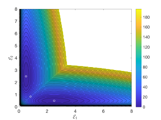
Figure 1. Energy landscape of $\mathcal{E}_{1}$ and $\mathcal{E}_{2}$ for $D=100$ and $\bar{\beta}=0.2$. The white circles show the location of the two minima and the saddle points, located approximately at (55) and (56), respectively. The potential is also capped at 200 for clarity.

For large $N$, the minima are approximately (that is, to leading order in $N^{-1}$) located at

(55) $$(\mathcal{E}_{1},\mathcal{E}_{2})=\frac{1}{2}(1,\bar{\beta}^{-1}),\quad\text{and}\quad(\mathcal{E}_{1},\mathcal{E}_{2})=\frac{1}{2}(\bar{\beta}^{-1},1)$$

with energy approximately given by $E_{m}=1+\log 2+\frac{1}{2}\log\bar{\beta}$ and the saddle point is approximately located at

(56) $$(\mathcal{E}_{1},\mathcal{E}_{2})=\bigl{(}(1+\bar{\beta})^{-1},(1+\bar{\beta})^{-1}\bigr{)}$$

with energy approximately given by $E_{s}=1+\log(1+\bar{\beta})$. Therefore, for large $D$, we can use results from large deviation theory to deduce that the smallest nonzero eigenvalue of the generator of (50) (that is, roughly, the inverse of mean first passage time between the minima) is log-asymptotically given by

(57) $$\bar{\lambda}_{1}\asymp\exp(-D\Delta E),\qquad\Delta E=E_{s}-E_{m}=\log(1+\bar{\beta})-\log 2+\frac{1}{2}\log\bar{\beta}^{-1}\qquad\text{as}\quad D\to\infty.$$

Therefore, for any $\bar{\beta}<1$ fixed, the system becomes increasingly metastable as $D$ gets larger. In particular, if we start with a configuration with $\mathcal{E}_{1}<\mathcal{E}_{2}$, it will take exponentially (in $D$) long time for the dynamics to reach the configurations with $\mathcal{E}_{1}>\mathcal{E}_{2}$. This means exponentially slow convergence to equilibrium, and shows that using two temperature is not sufficient in general.

5.2. The case with many temperatures

Consider now what happens with multiple temperatures, in which case a similar analysis as in the previous section can be done. In particular, the mixture potential (for the energies) has local minima at

(58) $$\mathcal{E}_{i}=\frac{1}{2\beta_{\sigma_{i}}}\qquad\text{for any permutation }\sigma,$$

whose energies scale as

(59) $$\frac{1}{2}\sum_{i}\log\beta_{i}+\frac{N}{2}(\log 2+1).$$

The saddle points are located at

(60) $$\begin{cases}\displaystyle\mathcal{E}_{i}=\frac{1}{2\beta_{\sigma_{i}}}\qquad\text{for}\;i\not=j,k\\ \mathcal{E}_{j}=\mathcal{E}_{k}=(\beta_{\sigma_{j}}+\beta_{\sigma_{k}})^{-1}\end{cases}$$

for any permutation $\sigma$ and any pair $j\not=k$, whose energies scale as

(61) $$\frac{1}{2}\sum_{i\not=j,k}\log\beta_{j}+\log(\beta_{j}+\beta_{k})+\frac{N-2}{2}\log 2+\frac{N}{2}.$$

Therefore the barrier scale as

(62) $$\Delta E_{j,k}=\log\biggl{(}\frac{\beta_{j}+\beta_{k}}{(\beta_{j}\beta_{k})^{1/2}}\biggr{)}-\log 2.$$

Assuming that $\beta_{1}>\beta_{2}>\ldots>\beta_{N}$, this indicates that we are more likely to see transition between minima lying on adjacent $\beta_{j}$s, and in order to keep all the rates equal (if we use Arrhenius formula such that rate is given by exponential of the energy barrier), we must have

(63) $$\frac{\beta_{j}+\beta_{j+1}}{(\beta_{j}\beta_{j+1})^{1/2}}=\text{cst}$$

for all $j=1,\ldots,N$. This agrees with the analysis based on transition state theory performed in our previous work [Lu2013], and shows that the optimal choice of temperature on the ladder should satisfy

(64) $$\frac{\beta_{j+1}}{\beta_{j}}=\Bigl{(}\frac{\beta_{N}}{\beta_{1}}\Bigr{)}^{1/(N-1)}$$

and that this ratio should be of order $1$. This indicates that using multiple temperature removes the energy barrier and hence makes convergence much faster.

6. Simulation of the stochastic switching dynamics

6.1. Direct simulation based on stochastic simulation algorithm

Here we present an exact implementation of the stochastic switching dynamics, assuming that we can integrate the Markov process corresponds to $\mathcal{L}_{\sigma}$ exactly. In practice, this integration often needs to be discretized, which will introduce some additional errors. We will discuss these later.

Given that at time $t$ the system is in the state $(\boldsymbol{X}(t),\sigma(t))$, the algorithm updates the state via the following steps:

1. Draw a random number $r\sim U([0,1])$;

2. Integrate $\boldsymbol{X}$ with the fixed $\sigma:=\sigma(t)$ to time $t+\tau$, such that

   $$r=\exp\biggr{(}-\nu\sum_{\sigma^{\prime}\neq\sigma}\int_{t}^{t+\tau}h_{\sigma\sigma^{\prime}}(\boldsymbol{X}(s))\,\,\mathrm{d}s\biggr{)},$$

   where $r$ is the random number drawn in Step 1;

3. Choose $\sigma(t+\tau)$ with probability

   $$\mathbb{P}\bigl{(}\sigma(t+\tau)=\sigma^{\prime}\mid\sigma,\tau\bigr{)}=\frac{h_{\sigma\sigma^{\prime}}(\boldsymbol{X}(t+\tau))}{\displaystyle\sum_{\widetilde{\sigma}\neq\sigma}h_{\sigma\widetilde{\sigma}}(\boldsymbol{X}(t+\tau))};$$

4. Update the time to $t+\tau$ and repeat till the target time.

If a large swapping rate $\nu$ is employed, the time lags $\tau$ will likely be rather small as their expectation is proportional to $\nu^{-1}$. In these situations, the stochastic switching dynamics exhibits two scales: the time scale of the diffusion process and that of the jumping process which is much faster. As a result, direct simulation by the algorithm discussed above is no longer efficient. This difficulty is in fact very similar to the one we encounter when numerically integrating SDEs with multiple time scales, for which a by-now standard idea is to explore the asymptotic limit explicitly to design a more efficient multiscale integrator. In what follows, we explore such an integrator, which was proposed in [TangLuAbramsVE] and fits the framework of the heterogeneous multiscale methods (HMM) [EEngquist:03, EVE:03, Weinan2007].

6.2. A multiscale integrator

The basic idea of the HMM integrator is to compute on-the-fly the scaling factor $R_{j}(\boldsymbol{X})$ in the limiting equation (41) for the slow variables $\boldsymbol{X}$ using short bursts of simulation of the fast process $\sigma$ – these simulations are performed in what is called the microsolver in HMM, whereas the routine used to evolve the slow variables is referred to as the macrosolver. The data generated by the microsolver is passed to the unknown coefficients for the macrosolver via an estimator. In the present context, the HMM scheme we will use works as follows:

Choose a time step $\Delta t$ appropriate for the simulation of the limiting SDEs (41) and pick a frequency $\nu$ such that $\nu\gg 1/\Delta t$ (for example $\nu=10^{2}/\Delta t-10^{3}/\Delta t$). Start the simulation with $\boldsymbol{X}^{(0)}=\boldsymbol{X}(0)$ and $\sigma^{(0)}=\sigma(0)$, and set $t_{0}=0$. Then for $k\geq 0$, we use the following 3-step iteration algorithm to update:

1. Microsolver: Evolve $\sigma^{(k)}$ via SSA from $t_{k}$ to $t_{k+1}:=t_{k}+\Delta t$ using the rate in (14) with $\boldsymbol{X}=\boldsymbol{X}^{(k)}$ fixed, that is: Set $\sigma^{(k,0)}=\sigma^{(k)}$, $t_{k,0}=t_{k}$, and for $l\geq 1$, do:

   1. Compute the lag to the next event via

      $$\tau_{l}=-\frac{\ln r}{\nu h_{\sigma^{(k,l-1)}}(\boldsymbol{X}^{(k)})}$$

      where $r$ is a random number uniformly distributed in the interval $(0,1)$ and $h_{\sigma}(\boldsymbol{X}^{(k)})=\sum_{\sigma^{\prime}\not=\sigma}h_{\sigma,\sigma^{\prime}}(\boldsymbol{X}^{(k)})$;

   2. Pick $\sigma_{k,l}$ with probability

      $$\mathbb{P}_{\sigma^{(k,l)}}=\frac{h_{\sigma^{(k,l-1)},\sigma^{(k,l)}}(\boldsymbol{X}^{(k)})}{h_{\sigma^{(k,l-1)}}(\boldsymbol{X}^{(k)})};$$

   3. Set $t_{k,l}=t_{k,l-1}+\tau_{l}$ and repeat till the first $L$ such that $t_{k,L}>t_{k}+\Delta t$; then set $\sigma^{(k+1)}=\sigma^{(k,L)}$ and reset $\tau_{L}=t_{k}+\Delta t-t_{k,L-1}$.

2. Estimator: Given the trajectory of $\sigma$, estimate $\eta_{j,i}(\boldsymbol{X}^{(k)})$ and $R_{j}(\boldsymbol{X}^{(k)})$ via

   $$\widehat{\eta}_{j,i}(\boldsymbol{X}^{(k)}) =\frac{1}{\Delta t}\int_{t_{k}}^{t_{k}+\Delta t}\mathbb{1}_{i=\sigma_{j}(s)}\,\mathrm{d}s$$

   $$=\frac{1}{\Delta t}\sum_{l=1}^{L}\tau_{l}\mathbb{1}_{i=\sigma^{(k,l)}_{j}},$$

   and

   $$\widehat{R}_{j}(\boldsymbol{X}^{(k)}) =\beta^{-1}\sum_{i}\frac{\beta_{i}}{\Delta t}\int_{t_{k}}^{t_{k}+\Delta t}\mathbb{1}_{i=\sigma_{j}(s)}\,\mathrm{d}s$$

   $$=\beta^{-1}\sum_{i}\beta_{i}\,\hat{\eta}_{j,i}(\boldsymbol{X}^{(k)}).$$

3. Macrosolver: Evolve $\boldsymbol{X}^{(k)}$ to $\boldsymbol{X}^{(k+1)}$ using one time-step of size $\Delta t$ in the numerical integrator for (41) with $R_{j}(\boldsymbol{X}^{(k)})$ replaced by the factor $\widehat{R}_{j}(\boldsymbol{X}^{(k)})$ calculated in the estimator. Then repeat the three steps above for each time-step $k$.

Remark.

It is useful to compare the above scheme with a time-splitting integrator for the dynamics of $(\boldsymbol{X}(t),\sigma(t))$, that is for time step size $\Delta t$, we alternate between evolving $\boldsymbol{X}(t)$ and $\sigma(t)$ while freezing the other component. More precisely, from $t_{k}$ to $t_{k+1}=t_{k}+\Delta t$ the algorithm updates the state via

1. Evolve $\sigma^{(k)}$ via SSA from $t_{k}$ to $t_{k+1}:=t_{k}+\Delta t$ using the rate in (14) with $\boldsymbol{X}=\boldsymbol{X}^{(k)}$ to get $\sigma^{(k+1)}$, using the similar procedure as the Microsolver in the multiscale integrator;

2. Evolve $\boldsymbol{X}^{(k)}$ to $\boldsymbol{X}^{(k+1)}$ using $\mathcal{L}_{\sigma^{(k+1)}}$, namely, if Euler-Maruyama scheme is used

   (65) $$\boldsymbol{x}_{j}^{(k+1)}=\boldsymbol{x}_{j}^{(k)}-\Delta t\beta^{-1}\beta_{\sigma_{j}^{(k+1)}}\nabla V(\boldsymbol{x}_{j}^{(k)})+\sqrt{2\beta^{-1}\Delta t}\;\eta_{j}^{(k)},$$

   where $\eta_{j}^{(k)}$ are i.i.d. standard Gaussian random variables.

The difference with the multiscale integrator lies in the evolution of $\boldsymbol{X}$, where the splitting scheme uses the current instance $\sigma^{(k+1)}$ while the multiscale integrator incorporates into the average of the coefficients. Since we are interested in the regime that the dynamics of $\sigma$ is much faster of $\boldsymbol{X}$, using the average is preferred as it is consistent with the $\nu\to\infty$ limit.

We will not go into details of the numerical analysis of the multiscale integrator here. Numerical analysis of HMM integrators in similar spirit can be found in [EEngquist:03, EVE:03, EVE:07, ELiuVE:05, TaoOwhadiMarsden2010, LuSpiliopoulos], the basic idea is to show that the scheme is consistent with the averaging limit as $\nu\to\infty$ by showing that the estimator gives a good approximation to $R_{j}(\boldsymbol{X})$.

7. Extension to simulated tempering

The analysis we have performed in the context of parallel tempering can be generalized to simulated tempering, as we briefly explain in this section. For a performance comparison between parallel and simulated tempering, we refer the readers to [Zhang2008].

We begin by noting that simulated tempering, in which we use one single replica but make the temperatures dynamically switch between $N$ values $\beta_{1}$, $\beta_{2}$, …, $\beta_{N}$, can be cast in a framework similar to that of the stochastic switching process discussed in Section 2. This amounts to assuming that the state space of the process is $\Omega^{N}\times\{1,\ldots,N\}$, and requiring that this process samples the joint equilibrium measure

(66) $$\pi(\,\mathrm{d}\boldsymbol{x},i)=\varrho(\boldsymbol{x},i)\,\mathrm{d}\boldsymbol{x},\qquad\text{with}\quad\varrho(\boldsymbol{x},i)=\frac{n_{i}e^{-\beta_{i}V(\boldsymbol{x})}}{\sum_{j}n_{j}Z_{\beta_{j}}}.$$

where $\{n_{i}\}_{i=1,\ldots,N}$ is a set of positive weights to be chosen a priori. To this end, the dynamics in $x$ given $i$ can be chosen as a time rescaled overdamped equation:

(67) $$\,\mathrm{d}\boldsymbol{x}(t)=-\beta^{-1}\beta_{i}\nabla V(\boldsymbol{x}(t))+\sqrt{2\beta^{-1}}\,\mathrm{d}\boldsymbol{W}_{t},$$

so that it samples

(68) $$\varrho(\boldsymbol{x}\mid i)=\frac{\varrho(\boldsymbol{x},i)}{\int_{\Omega}\varrho(\boldsymbol{y},i)\,\mathrm{d}\boldsymbol{y}}=Z_{\beta_{i}}^{-1}e^{-\beta_{i}V(\boldsymbol{x})}.$$

The jumping rate matrix between the temperature indices $i$ given $x$ can be chosen e.g.

(69) $$\nu k_{ij}(\boldsymbol{x})=\nu\min\Bigl{(}\frac{n_{j}}{n_{i}}e^{-(\beta_{j}-\beta_{i})V(\boldsymbol{x})},1\Bigr{)},\qquad i\not=j$$

with $k_{ii}(\boldsymbol{x})=-\sum_{j\not=i}k_{ij}$ so that the jumping process samples

(70) $$\varrho(i\mid\boldsymbol{x})=\frac{\varrho(\boldsymbol{x},i)}{\sum_{j=1}^{N}\varrho(\boldsymbol{x},j)}=\frac{n_{i}e^{-\beta_{i}V(\boldsymbol{x})}}{\sum_{j}n_{j}e^{-\beta_{j}V(\boldsymbol{x})}}.$$

Here $\nu$ is again an overall scaling parameter for the switching frequency. Other choices such as

(71) $$k_{ij}(\boldsymbol{x})=\frac{n_{j}}{n_{i}e^{-(\beta_{i}-\beta_{j})V(\boldsymbol{x})}+n_{j}},\qquad i\not=j,$$

or

(72) $$k_{ij}(\boldsymbol{x})=\sqrt{\frac{n_{j}}{n_{i}}}e^{-\frac{1}{2}(\beta_{j}-\beta_{i})V(\boldsymbol{x})},\qquad i\not=j,$$

are possible as well. The infinitesimal generator of the stochastic switching process $(\boldsymbol{x}(t),i(t))$ defined this way is given by

(73) $$(\mathcal{L}_{\nu}u)(\boldsymbol{x},i)=-\beta^{-1}\beta_{i}\nabla V(\boldsymbol{x})\cdot\nabla u(\boldsymbol{x},\beta)+\beta^{-1}\Delta u(\boldsymbol{x},\beta)+\nu\sum_{j\not=i}k_{i,j}(\boldsymbol{x})\bigl{(}u(\boldsymbol{x},j)-u(\boldsymbol{x},i)\bigr{)},$$

and it is an easy exercise to show that its invariant measure is indeed (66).

In terms of calculating expectations, in the context of simulated tempering we can use

(74) $$\left\langle A\right\rangle_{\beta_{k}} \equiv\int_{\Omega}A(\boldsymbol{x})\rho_{\beta_{k}}(\boldsymbol{x})\,\mathrm{d}\boldsymbol{x}$$

$$=\int_{\Omega}A(\boldsymbol{x})g_{k}(\boldsymbol{x})\varrho(x)\,\mathrm{d}\boldsymbol{x}$$

where $\varrho(\boldsymbol{x})$ is the marginal of $\varrho(\boldsymbol{x},i)$ on $\boldsymbol{x}$:

(75) $$\varrho(\boldsymbol{x})=\sum_{i=1}^{N}\varrho(\boldsymbol{x},i)=\frac{\sum_{i=1}^{N}n_{i}e^{-\beta_{i}V(\boldsymbol{x})}}{\sum_{i=1}^{N}n_{i}Z_{\beta_{i}}},$$

and we defined

(76) $$g_{k}(\boldsymbol{x})=\frac{\rho_{\beta_{k}}(\boldsymbol{x})}{\varrho(\boldsymbol{x})}=\frac{Z_{\beta_{k}}^{-1}e^{-\beta_{k}V(\boldsymbol{x})}\sum_{j=1}^{N}n_{j}Z_{\beta_{j}}}{\sum_{j=1}^{N}n_{j}e^{-\beta_{j}V(\boldsymbol{x})}}.$$

These expressions show the main (and well-known) difficulty one is faced when using simulated tempering: even though it looks simpler than simulated tempering because it involves a single replica, it requires one to learn the partition functions $Z_{\beta_{i}}$ to calculate expectations (in contrast, parallel tempering does not require this).

Setting this difficulty inside, an argument similar to the one presented in Section 3 indicates that the large deviation rate functional for the empirical measure of the process with generator (73) is the sum of the terms, the first of which is independent of $\nu$ and the second proportional to $\nu$. This indicates that, in the context of simulating tempering too, it is optimal to take the limit as $\nu\to\infty$ (which we will refer to as the ‘infinite switching limit’). In this limit, it is easy to show using averaging arguments similar to those presented in Section 4, that the process $\boldsymbol{x}(t)$ converges to the solution of the following effective equation

(77) $$\,\mathrm{d}\boldsymbol{x}(t)=-\beta^{-1}\widebar{\beta}(\boldsymbol{x}(t))\nabla V(\boldsymbol{x}(t))+\sqrt{2\beta^{-1}}\,\mathrm{d}\boldsymbol{W}_{t},$$

where we defined

(78) $$\widebar{\beta}(\boldsymbol{x})=\sum_{i=1}^{N}\beta_{i}\varrho(i\mid\boldsymbol{x})=\frac{\sum_{i=1}^{N}\beta_{i}n_{i}e^{-\beta_{i}V(\boldsymbol{x})}}{\sum_{i=1}^{N}n_{i}e^{-\beta_{i}V(\boldsymbol{x})}}.$$

This equation is in principle much easier to simulate than the corresponding effective equation (41) obtained in the infinite switching limit of paralel tempering, since the sum in (78) involves $N$ terms instead of $N!$ (and hence can be evaluated straightforwardly even for large $N$). However, the efficiency boost of the method depends crucially on the choice of the weights $n_{i}$. It has been argued that the optimal choice is to take $n_{i}=Z_{\beta_{i}}^{-1}$, but, unfortunately, these partition functions are unknown a priori (which brings us back to the issue with the estimator (74) for the expectations). How to go around these difficulties (and justify the optimality of the choice $n_{i}=Z_{\beta_{i}}^{-1}$ starting from the effective equation in (77)) will be discussed elsewhere.

8. Concluding remarks

We have shown how a formulation of parallel tempering as a stochastic switching process for the coupled dynamics of replica configuration and temperature permutation naturally leads to considering these equations in the infinite swapping limit. Indeed this can be justified from the additive structure of the rate functional for the empirical measure of the process, using tools from large deviation theory as originally proposed in [Plattner2011] and further justified in [DupuisLiu:2015]. This observation suggests to simulate directly the effective equation that emerges in this limit . Unfortunately, this is no trivial task because the direct calculation of the coefficients in this equation involves sums over all possible permutations of the temperatures. Clearly this is only doable if the number of temperatures/replicas is small, which is a set-up in which parallel tempering leads to no significant boost in efficiency. This observation is common knowledge for practitioners of parallel tempering, and is usually justified by showing that many temperatures are required to get a significant acceptance rate of the temperature swaps. Within the infinite swapping limit, we arrive at the same conclusion, but from a different viewpoint: as we showed here, it is necessary to use many temperatures in order to eliminate the free energy barriers on the mixture potential.

Once one realizes that the effective equation emerging in the infinite swapping limit must be operated with many temperatures, the question arises as how to do so in practice. Following the suggestion made in [TangLuAbramsVE], we showed here that it can be done using multiscale integrators such as HMM. These schemes are straightforward generalization of those traditionally used in parallel tempering, and we therefore they should be useful to improve the efficiency of this method with rather minimal modifications of the existing codes. Alternatively, we showed that one can use similar ideas in the context of simulated tempering, in which case the limiting equation that arise in the infinite switching limit is simpler.