Evidence of ghost suppression in gluon mass dynamics

Abstract

In this work we study the impact that the ghost sector of pure Yang-Mills theories may have on the generation of a dynamical gauge boson mass, which hinges on the appearance of massless poles in the fundamental vertices of the theory, and the subsequent realization of the well-known Schwinger mechanism. The process responsible for the formation of such structures is itself dynamical in nature, and is governed by a set of Bethe-Salpeter type of integral equations. While in previous studies the presence of massless poles was assumed to be exclusively associated with the background-gauge three-gluon vertex, in the present analysis we allow them to appear also in the corresponding ghost-gluon vertex. The full analysis of the resulting Bethe-Salpeter system reveals that the contribution of the poles associated with the ghost-gluon vertex are particularly suppressed, their sole discernible effect being a slight modification in the running of the gluon mass, for momenta larger than a few GeV. In addition, we examine the behavior of the (background-gauge) ghost-gluon vertex in the limit of vanishing ghost momentum, and derive the corresponding version of Taylor’s theorem. These considerations, together with a suitable Ansatz, permit us the full reconstruction of the pole sector of the two vertices involved.

I Introduction

The nonperturbative generation of an effective gluon mass has attracted particular attention in the last decade, being identified as one of the fundamental emergent phenomena produced by the intricate gauge-sector dynamics of QCD Cloet and Roberts (2014); Roberts (2017); Roberts and Mezrag (2017). As has been advocated in a series of works Aguilar and Papavassiliou (2006); Aguilar et al. (2008, 2012); Ibañez and Papavassiliou (2013); Aguilar et al. (2016), the appearance of such a (momentum-dependent) mass Cornwall (1982), $m^{2}(q^{2})$, is inextricably connected with the infrared finiteness of the gluon propagator, $\Delta(q^{2})$, and the ghost dressing function, $F(q^{2})$, observed in a variety of large-volume lattice simulations Cucchieri and Mendes (2007, 2008, 2010); Bowman et al. (2007); Bogolubsky et al. (2009); Oliveira and Silva (2009); Ayala et al. (2012); Bicudo et al. (2015). Even though these paradigm-shifting lattice results have been explained and interpreted within a plethora of diverse theoretical approaches Cornwall (1982); Lavelle (1991); Halzen et al. (1993); Philipsen (2002); Szczepaniak and Swanson (2002); Aguilar and Natale (2004); Aguilar and Papavassiliou (2006); Kondo (2006); Braun et al. (2010); Epple et al. (2008); Aguilar et al. (2008); Boucaud et al. (2008); Dudal et al. (2008); Fischer et al. (2009); Aguilar et al. (2009); Rodriguez-Quintero (2011); Campagnari and Reinhardt (2010); Tissier and Wschebor (2010); Kondo (2010); Pennington and Wilson (2011); Watson and Reinhardt (2012); Kondo (2011); Serreau and Tissier (2012); Strauss et al. (2012); Cloet and Roberts (2014); Siringo (2014); Binosi et al. (2015); Aguilar et al. (2015); Huber (2015); Capri et al. (2015); Binosi et al. (2017); Glazek et al. (2017); Gao et al. (2017), in the present work we employ the formal framework that emerges from the fusion between the pinch-technique (PT) Cornwall (1982); Cornwall and Papavassiliou (1989); Pilaftsis (1997); Binosi and Papavassiliou (2002a, 2004, 2009) with the background-field method (BFM) Abbott (1981), known as “PT-BFM scheme” Aguilar and Papavassiliou (2006); Binosi and Papavassiliou (2008a, b).

The set of basic ideas underlying the approach put forth in Aguilar et al. (2012); Ibañez and Papavassiliou (2013), and more recently in Aguilar et al. (2016), may be summarized as follows. At the level of the Schwinger-Dyson equation (SDE) that governs the dynamics of the gluon propagator within the PT-BFM scheme, the masslessness of the gluon is enforced nonperturbatively by means of a special integral identity (“seagull” identity Aguilar and Papavassiliou (2010); Aguilar et al. (2016)). This identity is triggered by the special (Abelian) Slavnov-Taylor identities (STIs) satisfied by the fundamental vertices appearing in the diagrammatic expansion of the gluon SDE, enforcing the exact result $\Delta^{-1}(0)=0$. The action of the seagull identity may be circumvented, allowing for the possibility $\Delta^{-1}(0)\neq 0$, only if the well-known Schwinger mechanism Schwinger (1962a, b) is triggered Jackiw and Johnson (1973); Smit (1974); Eichten and Feinberg (1974); Poggio et al. (1975). The activation of this latter mechanism, in turn, requires the presence of longitudinally coupled massless poles, i.e., of the generic form $(q^{\mu}/q^{2})\widetilde{C}(q,r,p)$, in the aforementioned vertices entering in the gluon SDE.

The origin of these poles is dynamical rather than kinematic, and may be traced back to the formation of tightly bound colored excitations; in fact, within this picture, the terms $\widetilde{C}$ may be identified with the “bound-state wave functions” of these excitations. The quantities relevant for the generation of a gluon mass and the determination of its momentum dependence are the partial derivatives of the $\widetilde{C}(q,r,p)$ as $q\to 0$, to be generically denoted by $\widetilde{C}^{\prime}(r^{2})$; their evolution, in turn, is controlled by a system of coupled homogeneous linear Bethe-Salpeter equations (BSEs) Jackiw and Johnson (1973); Smit (1974); Eichten and Feinberg (1974); Poggio et al. (1975).

Even though, in principle, all fundamental vertices entering into the gluon SDE, i.e., the three-gluon, ghost-gluon, and four-gluon vertex, may develop such poles, one of the main simplifications implemented in all previous studies is the assumption that the dominant effect originates from the three-gluon vertex, and that all contributions from the pole parts of the remaining vertices are numerically subleading. This assumption, in turn, reduces dramatically the level of technical complexity, converting the system of coupled BSEs into one single dynamical equation (in the Landau gauge). In the present work we partially relax this basic assumption by including massless poles also in the ghost-gluon vertex, $\widetilde{\Gamma}_{\mu}$, and studying in detail how the results previously obtained are affected by their presence.

The analysis necessary for addressing the aforementioned dynamical question is significantly more complicated than that of Aguilar et al. (2012); Binosi and Papavassiliou (2017), mainly due to the fact that the pole formation is now governed by a system of two coupled integral equations. Specifically, the resulting system of BSEs involves as unknown quantities the derivative of the wave function of the pole in the three-gluon vertex, $\widetilde{\Gamma}_{\mu\alpha\beta}$, to be denoted by $\widetilde{C}_{\mathrm{gl}}^{\prime}(r^{2})$, and the corresponding quantity in $\widetilde{\Gamma}_{\mu}$, to be denoted by $\widetilde{C}_{\mathrm{gh}}^{\prime}(r^{2})$.

These two quantities affect the gluon dynamics in rather distinct ways. To begin with, both $\widetilde{C}_{\mathrm{gl}}^{\prime}(r^{2})$ and $\widetilde{C}_{\mathrm{gh}}^{\prime}(r^{2})$ enter in the formula that determines the value of $\Delta^{-1}(0)$ [see Eq. (19)]; however, their relative contribution can be vastly different, even if it turned out that $\widetilde{C}_{\mathrm{gl}}^{\prime}(r^{2})\simeq\widetilde{C}_{\mathrm{gh}}^{\prime}(r^{2})$, because they are convoluted with completely different structures. Moreover, as has been shown first in Aguilar et al. (2012) and recently revisited in Binosi and Papavassiliou (2017), the running gluon mass, $m^{2}(q^{2})$, is entirely determined from the form of $\widetilde{C}_{\mathrm{gl}}^{\prime}(r^{2})$. Therefore, the way that $\widetilde{C}_{\mathrm{gh}}^{\prime}(r^{2})$ could affect $m^{2}(q^{2})$ is indirect, depending on the difference between the $\widetilde{C}_{\mathrm{gl}}^{\prime}(r^{2})$ found from the (single) BSE when $\widetilde{C}_{\mathrm{gh}}^{\prime}(r^{2})$ is assumed to vanish identically, as was done previously Aguilar et al. (2012); Binosi and Papavassiliou (2017), and the $\widetilde{C}_{\mathrm{gl}}^{\prime}(r^{2})$ obtained by actually solving the coupled BSE system, as we do here.

The full analysis of the BSE system carried out in the present work reveals that $\widetilde{C}_{\mathrm{gh}}^{\prime}(r^{2})$ is considerably smaller than $\widetilde{C}_{\mathrm{gl}}^{\prime}(r^{2})$. Specifically, when all quantities entering into the kernels of the BSE system have been renormalized using the momentum subtraction scheme (MOM) at the point $\mu=4.3$ GeV, the relative size between the two quantities is approximately $\widetilde{C}_{\mathrm{gh}}^{\prime}(r^{2})/\widetilde{C}_{\mathrm{gl}}^{\prime}(r^{2})\simeq 1/5$. As a result, the substitution of $\widetilde{C}_{\mathrm{gl}}^{\prime}(r^{2})$ and $\widetilde{C}_{\mathrm{gh}}^{\prime}(r^{2})$ into the corresponding integrals that determine $\Delta^{-1}(0)$ shows that the effect stemming from $\widetilde{C}_{\mathrm{gh}}^{\prime}(r^{2})$ is practically negligible. This conclusion may be restated in terms of the quadratic equation for the strong coupling $\alpha_{s}$, introduced in Binosi and Papavassiliou (2017); specifically, the value of $\alpha_{s}$ that emerges from the combination of the BSE and the SDE remains practically unchanged in the presence of the nonvanishing, but rather small, $\widetilde{C}_{\mathrm{gh}}^{\prime}(r^{2})$. The only place where $\widetilde{C}_{\mathrm{gh}}^{\prime}(r^{2})$ makes a small but discernible difference is in the running of $m^{2}(q^{2})$, in the region of momenta more than a few GeV. In particular, the deviation from the exact power-law running is controlled by the value of the exponent $p$, which changes from the value $p=0.1$ when $\widetilde{C}_{\mathrm{gh}}^{\prime}(r^{2})$ is neglected Binosi and Papavassiliou (2017) to the value $p=0.24$ when $\widetilde{C}_{\mathrm{gh}}^{\prime}(r^{2})$ is included. Thus, the overall conclusion of this work is that the effects of the ghost sector, in the sense described above, do not modify appreciably the dynamics responsible for the generation of an effective gluon mass.

In addition to the findings just mentioned, the present study addresses certain aspects related to the structure and behaviour of $\widetilde{\Gamma}_{\mu}$, which are theoretically interesting and novel, and furnish further insights into the underlying mass-generation mechanism. Specifically, as is well-known, in the limit of vanishing ghost momentum, the form-factors of the conventional ghost-gluon vertex, ${\Gamma}_{\mu}$, satisfy a special exact relation, known as Taylor’s theorem Taylor (1971). In this work we derive the corresponding relation for $\widetilde{\Gamma}_{\mu}$, using three vastly different approaches. The form of Taylor’s theorem that emerges is clearly different from the standard case, involving the ghost dressing function $F(q^{2})$ as its new main ingredient.

Furthermore, the structure of $\widetilde{\Gamma}_{\mu}$ is scrutinized, placing particular emphasis on the way that the fundamental (Abelian) STI is realized in the presence of a longitudinally coupled pole term. In fact, it is shown that through an appropriate rearrangement of its form factors, consistent with the (newly derived) version of Taylor’s theorem, the effect of the pole may be reabsorbed in the transverse (automatically conserved) part of the vertex. The above considerations are not without practical interest, since they allow us to fully determine (under some mild assumptions) the entire function $\widetilde{C}_{\mathrm{gh}}(q,r,p)$ from the knowledge of $\widetilde{C}_{\mathrm{gh}}^{\prime}(r^{2})$.

The article is organized as follows. In Sec. II we review the basic formalism employed in this work, with particular emphasis on the way the massless poles enter into the vertices, and the special way the corresponding STIs are satisfied in their presence. Then, in Sec. III we derive the version of Taylor’s theorem applicable to $\widetilde{\Gamma}_{\mu}$, using three different procedures: $(i)$ the STI that $\widetilde{\Gamma}_{\mu}$ satisfies; $(ii)$ the SDE of $\widetilde{\Gamma}_{\mu}$, and $(iii)$ an exact relation connecting $\widetilde{\Gamma}_{\mu}$ with ${\Gamma}_{\mu}$, known as “background-quantum identity” (BQI) Binosi and Papavassiliou (2008b). In Sec. IV we offer a new perspective on the way that the STI of $\widetilde{\Gamma}_{\mu}$ is enforced for a nonvanishing $\widetilde{C}_{\mathrm{gh}}(q,r,p)$, as well as the constraints imposed on it from Taylor’s theorem. The upshot of this analysis is the demonstration that one may reinterpret the action of the longitudinally coupled pole as a corresponding pole contribution in the transverse part of $\widetilde{\Gamma}_{\mu}$. In addition, using the above results, we present a simple Ansatz for $\widetilde{C}_{\mathrm{gh}}(q,r,p)$, which allows its full reconstruction, once $\widetilde{C}_{\mathrm{gh}}^{\prime}(r^{2})$ has been determined. In Sec. V we derive the BSE system that governs $\widetilde{C}_{\mathrm{gl}}^{\prime}(r^{2})$ and $\widetilde{C}_{\mathrm{gh}}^{\prime}(r^{2})$. Then, in Sec. VI we present the numerical analysis, and establish the subleading nature of the ghost-related contributions. Finally, in Sec. VII we present our conclusions.

II Gluon mass from vertices with massless poles

For an SU(3) pure Yang-Mills theory (no dynamical quarks) quantized in the Landau gauge, the gluon and ghost propagators have the form (we factor out the trivial color structure $\delta^{ab}$)

$$\Delta_{\mu\nu}(q) =-i\Delta(q^{2})P_{\mu\nu}(q);\qquad P_{\mu\nu}(q)=g_{\mu\nu}-\frac{q_{\mu}q_{\nu}}{q^{2}},$$

$$D(q^{2}) =i\frac{F(q^{2})}{q^{2}}.$$ (1)

In the formulas above, $\Delta(q^{2})$ is related to the scalar form factor of the gluon self-energy $\Pi_{\mu\nu}(q)=P_{\mu\nu}(q)\Pi(q^{2})$ through $\Delta^{-1}(q^{2})=q^{2}+i\Pi(q^{2})$, while $F(q^{2})$ represents the so-called ghost dressing function; at tree-level $\Delta^{(0)}(q^{2})=1/q^{2}$ and $F^{(0)}(q^{2})=1$.

Within the PT-BFM framework that we employ in the ensuing analysis, the SDE of $\Delta(q^{2})$ is expressed in terms of the $QB$ self-energy $\widetilde{\Pi}_{\mu\nu}(q)$, namely

$$\Delta^{-1}(q^{2})P_{\mu\nu}(q) =\frac{q^{2}P_{\mu\nu}(q)+i\widetilde{\Pi}_{\mu\nu}(q)}{1+G(q^{2})},$$ (2)

where $G(q^{2})$ is the $g_{\mu\nu}$ component of a special two-point function Binosi and Papavassiliou (2002b), related to the ghost dressing function through the equation $1+G(0)=F^{-1}(0)$, see also Eq. (50) below Grassi et al. (2004); Aguilar et al. (2009).

Expressing the gluon SDE in terms of $\widetilde{\Pi}_{\mu\nu}(q)$ rather than $\Pi_{\mu\nu}(q)$ entails the advantage that, when contracted from the side of the $B$-gluon, each fully dressed vertex satisfies a linear (Abelian-like) Slavnov-Taylor identity (STI). In particular, the $BQ^{2}$ vertex $\widetilde{\Gamma}_{\mu\alpha\beta}$ and the $Bc\bar{c}$ vertex $\widetilde{\Gamma}_{\mu}$ satisfy (color omitted and all momenta entering)

$$q^{\mu}\widetilde{\Gamma}_{\mu\alpha\beta}(q,r,p)=i\Delta_{\alpha\beta}^{-1}(r)-i\Delta_{\alpha\beta}^{-1}(p),$$ (3)

$$q^{\mu}\widetilde{\Gamma}_{\mu}(q,r,p)=iD^{-1}(r^{2})-iD^{-1}(p^{2}),$$ (4)

whereas for the $BQ^{3}$ vertex we have

$$q^{\mu}\widetilde{\Gamma}^{mnrs}_{\mu\alpha\beta\gamma}(q,r,p,t) =f^{mse}f^{ern}\Gamma_{\alpha\beta\gamma}(r,p,q+t)+f^{mne}f^{esr}\Gamma_{\beta\gamma\alpha}(p,t,q+r)$$

$$+f^{mre}f^{ens}\Gamma_{\gamma\alpha\beta}(t,r,q+p).$$ (5)

Recently, it has been shown that if the vertices carrying the $B$ leg do not contain massless poles of the type $1/q^{2}$, then the $\Delta(q^{2})$ governed by Eq. (2) remains rigorously massless Aguilar et al. (2016). The demonstration relies on the subtle interplay between the Ward-Takahashi identities (WTIs), satisfied by the vertices as $q\to 0$, and an integral relation known as the “seagull identity” Aguilar and Papavassiliou (2010); Aguilar et al. (2016). In fact, in the absence of massless poles, the Taylor expansion of both sides of Eqs. (3) and (4) generates the corresponding WTIs

$$\widetilde{\Gamma}_{\mu\alpha\beta}(0,r,-r)=-i\frac{\partial}{\partial r^{\mu}}\Delta^{-1}_{\alpha\beta}(r),$$ (6)

$$\widetilde{\Gamma}_{\mu}(0,r,-r)=-i\frac{\partial}{\partial r^{\mu}}D^{-1}(r^{2}),$$ (7)

and

$$\widetilde{\Gamma}^{mnrs}_{\mu\alpha\beta\gamma}(0,-r,-p,r+p) =-\left(f^{mne}f^{esr}\frac{\partial}{\partial r^{\mu}}+f^{mre}f^{ens}\frac{\partial}{\partial p^{\mu}}\right)\Gamma_{\alpha\beta\gamma}(-r,-p,r+p).$$ (8)

Using these expressions in evaluating the gluon SDE, yields then

$$\Delta^{-1}(0) =\underbrace{\int_{k}\frac{\partial}{\partial k_{\mu}}{\cal F}_{\mu}(k)=0}_{\rm seagull\,\,identity},$$ (9)

where

$${\cal F}_{\mu}(k) =k_{\mu}{\cal F}(k^{2}); {\cal F}(k^{2})=\Delta(k^{2})[c_{1}+c_{2}Y(k^{2})]+c_{3}D(k^{2}),$$ (10)

with $c_{1},c_{2},c_{3}\neq 0$, and

$$Y(k^{2}) =\frac{1}{(d-1)}\frac{k_{\alpha}}{k^{2}}\!\int_{\ell}\!\Delta^{\alpha\rho}(\ell)\Delta^{\beta\sigma}(\ell+k)\Gamma_{\sigma\rho\beta}(-\ell-k,\ell,k).$$ (11)

This result may be circumvented by relaxing the assumption made when deriving Eqs. (3) and (4), allowing the vertices to contain longitudinally coupled $1/q^{2}$ poles; their inclusion, in turn, triggers the Schwinger mechanism Schwinger (1962a, b), finally enabling the generation of a gauge boson mass Jackiw and Johnson (1973); Smit (1974); Eichten and Feinberg (1974); Poggio et al. (1975).

Neglecting effects stemming from poles associated with the four-gluon vertex, the $BQ^{2}$ and $Bc\bar{c}$ vertices will then take the form

$$\widetilde{\Gamma}_{\mu\alpha\beta}(q,r,p) =\widetilde{\Gamma}^{\mathrm{np}}_{\mu\alpha\beta}(q,r,p)+i\frac{q_{\mu}}{q^{2}}\widetilde{C}_{\alpha\beta}(q,r,p),$$ (12)

$$\widetilde{\Gamma}_{\mu}(q,r,p) =\widetilde{\Gamma}^{\mathrm{np}}_{\mu}(q,r,p)+i\frac{q_{\mu}}{q^{2}}\widetilde{C}_{\mathrm{gh}}(q,r,p),$$ (13)

where the superscript “np” stands for “no-pole”, whereas $\widetilde{C}_{\alpha\beta}$ and $\widetilde{C}_{\mathrm{gh}}$ represents the bound-state gluon-gluon and gluon-ghost wave functions, respectively Jackiw and Johnson (1973); Eichten and Feinberg (1974); Poggio et al. (1975).

Next, in order to preserve the BRST symmetry of the theory, we demand that all STIs maintain their exact form in the presence of these poles; therefore, Eqs. (3) and (4) will now read

$$q^{\mu}\widetilde{\Gamma}^{\mathrm{np}}_{\mu\alpha\beta}(q,r,p)+\widetilde{C}_{\alpha\beta}(q,r,p)=i\Delta_{\alpha\beta}^{-1}(r)-i\Delta_{\alpha\beta}^{-1}(p),$$ (14)

$$q^{\mu}\widetilde{\Gamma}^{\mathrm{np}}_{\mu}(q,r,p)+\widetilde{C}_{\mathrm{gh}}(q,r,p)=iD^{-1}(r^{2})-iD^{-1}(p^{2}).$$ (15)

Taking the limit of Eqs. (14) and (15) as $q\to 0$ on both sides, matching the zeroth order in $q$ yields the conditions

$$\widetilde{C}_{\alpha\beta}(0,r,-r) =0; \widetilde{C}_{\mathrm{gh}}(0,r,-r) =0,$$ (16)

whereas the terms linear in $q$ furnish a modified set of WTIs, namely

$$\widetilde{\Gamma}^{\mathrm{np}}_{\mu\alpha\beta}(0,r,-r)=-i\frac{\partial}{\partial r^{\mu}}\Delta^{-1}_{\alpha\beta}(r)-\left\{\frac{\partial}{\partial q^{\mu}}\widetilde{C}_{\alpha\beta}(q,r,-r-q)\right\}_{q=0},$$ (17)

$$\widetilde{\Gamma}^{\mathrm{np}}_{\mu}(0,r,-r)=-i\frac{\partial}{\partial r^{\mu}}D^{-1}(r^{2})-\left\{\frac{\partial}{\partial q^{\mu}}\widetilde{C}_{\mathrm{gh}}(q,r,-r-q)\right\}_{q=0}.$$ (18)

The presence of the second term on the r.h.s. of Eqs. (17) and (18) has far-reaching consequences for the infrared behavior of $\Delta(q^{2})$. Specifically, a repetition of the steps leading to Eq. (9) reveals that, whereas the first terms on the r.h.s. of these equations reproduces again Eq. (9) (and their contributions thus vanish), the second terms survive, giving

$$\Delta^{-1}(0) =\frac{3}{2}g^{2}C_{A}F(0)\left\{\int_{k}k^{2}\Delta^{2}(k^{2})\left[1-\frac{3}{2}g^{2}C_{A}Y(k^{2})\right]\widetilde{C}_{\mathrm{gl}}^{\prime}(k^{2})-\frac{1}{3}\int_{k}k^{2}D^{2}(k^{2})\widetilde{C}_{\mathrm{gh}}^{\prime}(k^{2})\right\},$$ (19)

where $C_{A}$ is the Casimir eigenvalue of the adjoint representation [$N$ for SU($N$)], $\widetilde{C}_{\mathrm{gl}}$ is the form factor of $g_{\alpha\beta}$ in the tensorial decomposition of $\widetilde{C}_{\alpha\beta}$, and

$$C_{i}^{\prime}(k^{2})=\lim_{q\to 0}\left\{\frac{\partial\widetilde{C}_{i}(q,k,-k-q)}{\partial(k+q)^{2}}\right\},\quad i=\mathrm{gl},\ \mathrm{gh}.$$ (20)

As we see from Eq. (19), a necessary condition for $\Delta^{-1}(0)$ to acquire a nonvanishing value is that at least one of the $\widetilde{C}_{\mathrm{gl}}^{\prime}$ and $\widetilde{C}_{\mathrm{gh}}^{\prime}$ does not vanish identically; in addition, $\widetilde{C}_{\mathrm{gl}}^{\prime}$ and $\widetilde{C}_{\mathrm{gh}}^{\prime}$ must decrease sufficiently rapidly in the ultraviolet, in order for the integrals in Eq. (19) to give a (positive) finite value.

Let us conclude this section by linking the non-vanishing of $\widetilde{C}_{\mathrm{gl}}^{\prime}$ to the generation of a running gluon mass of the type familiar from the quark case Cloet and Roberts (2014). The infrared saturation of the gluon propagator suggests the physical parametrization $\Delta^{-1}(q^{2})=q^{2}J(q^{2})+m^{2}(q^{2})$ where $J(q^{2})\sim\ln q^{2}$ at most, and $m^{2}(0)\neq 0$. Then the modified gluon STI (14) will make it natural to associate the $J$ terms with the $q^{\mu}\widetilde{\Gamma}^{\mathrm{np}}_{\mu\alpha\beta}$ on the left-hand side (l.h.s.), and, correspondingly,

$$\widetilde{C}_{\alpha\beta}(q,r,p) =m^{2}(p^{2})P_{\alpha\beta}(p)-m^{2}(r^{2})P_{\alpha\beta}(r).$$ (21)

Focusing on the $g_{\alpha\beta}$ components of Eq. (21), we obtain Aguilar et al. (2012)

$$\widetilde{C}_{\mathrm{gl}}(q,r,p)=m^{2}(r^{2})-m^{2}(p^{2})\quad\underset{q\to 0}{\Longrightarrow}\quad\widetilde{C}_{\mathrm{gl}}^{\prime}(r^{2})=\frac{{\rm d}m^{2}(r^{2})}{{\rm d}r^{2}}.$$ (22)

Then, upon integration, we obtain

$$m^{2}(q^{2})=\Delta^{-1}(0)+\int_{0}^{q^{2}}\!\!{\rm d}y\,\widetilde{C}_{\mathrm{gl}}^{\prime}(y),$$ (23)

thus establishing the announced link between $\widetilde{C}_{\mathrm{gl}}^{\prime}$ and a dynamically generated gluon mass Binosi et al. (2012).

III Taylor’s theorem for the PT-BFM vertex $\widetilde{\Gamma}_{\mu}(q,r,p)$

Taylor’s theorem Taylor (1971), which is particular to the Landau gauge, establishes an exact constraint on the form factors comprising the conventional ghost-gluon vertex (all momenta entering as usual)

$$i{\Gamma}_{c^{n}Q^{a}_{\mu}\bar{c}^{m}}(p,q,r) =gf^{amn}{\Gamma}_{\mu}(q,r,p); {\Gamma}^{(0)}_{\mu}(q,r,p) =-r_{\mu},$$ (24)

in the limit of vanishing ghost momentum ($p=0$). In this section, after briefly recalling how this theorem follows directly from the SDE satisfied by ${\Gamma}_{\mu}$, we derive the analogous relation for the BFM vertex

$$i{\Gamma}_{c^{n}B^{a}_{\mu}\bar{c}^{m}}(p,q,r) =gf^{amn}\widetilde{\Gamma}_{\mu}(q,r,p); \widetilde{\Gamma}^{(0)}_{\mu}(q,r,p) =(p-r)_{\mu},$$ (25)

using three different methods: $(i)$ the Abelian STI (4), $(ii)$ the BQI that connects ${\Gamma}_{\mu}$ with $\widetilde{\Gamma}_{\mu}$, and $(iii)$ the SDE satisfied by $\widetilde{\Gamma}_{\mu}$.

III.1 Taylor’s theorem for ${\Gamma}_{\mu}(q,r,p)$

The most compact version of Taylor’s theorem may be obtained by using the gluon and ghost momenta ($q$ and $p$, respectively) for the tensorial decomposition of ${\Gamma}_{\mu}$, namely

$${\Gamma}_{\mu}(q,r,p)=A(q,r,p)q_{\mu}+B(q,r,p)p_{\mu}.$$ (26)

From the SDE of Fig. 1, we have that

$$gf^{amn}{\Gamma}_{\mu}(q,r,p)=-gf^{amn}r_{\mu}+gf^{dbn}\int_{k}(k+p)_{\rho}\Delta^{\rho\sigma}(k)D(k+p){\cal Q}^{damb}_{\sigma\mu}(-k,q,r,k+p),$$ (27)

where ${\cal Q}^{damb}_{\sigma\mu}$ represents the $QQc\bar{c}$ kernel appearing in diagram $(b)$ of that figure. Evidently, in the Landau gauge, $(k+p)_{\rho}\Delta^{\rho\sigma}(k)=p_{\rho}\Delta^{\rho\sigma}(k)$, so that the entire contribution from the second term in Eq. (27) vanishes when $p\to 0$. Thus, in the Taylor limit, Eq. (27) yields simply

$${\Gamma}_{\mu}(q,-q,0)=q_{\mu},$$ (28)

while, from Eq. (26), in the same limit, we have that

$${\Gamma}_{\mu}(q,-q,0)=A(q,-q,0)q_{\mu}.$$ (29)

Therefore, from Eqs. (28) and (29) one obtains the known result

$$A(q,-q,0)=1.$$ (30)

Notice that if instead one expresses ${\Gamma}_{\mu}(q,r,p)$ in terms of $q$ and $r$, namely

$${\Gamma}_{\mu}(q,r,p)=A_{1}(q,r,p)q_{\mu}-B_{1}(q,r,p)r_{\mu},$$ (31)

we have that $A(q,r,p)=A_{1}(q,r,p)+B_{1}(q,r,p)$ and $B(q,r,p)=B_{1}(q,r,p)$, so that Eq. (30) yields

$$A_{1}(q,-q,0)+B_{1}(q,-q,0)=1,$$ (32)

which is the form of the theorem employed in previous works Aguilar et al. (2009, 2013).

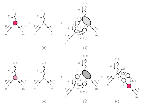
Figure 1: The SDE satisfied by the gluon-ghost conventional (top) and BFM vertex (bottom). In this latter case an extra term $(\widetilde{c})$ appears, due to the presence of the additional BFM tree-level coupling $BQc{\bar{c}}$.

III.2 Taylor’s theorem for $\widetilde{\Gamma}_{\mu}(q,r,p)$ from its STI

Let us now turn to the vertex $\widetilde{\Gamma}_{\mu}(q,r,p)$, and consider its tensorial decomposition analogous to Eq. (26),

$${\widetilde{\Gamma}}_{\mu}(q,r,p)={\widetilde{A}}(q,r,p)q_{\mu}+{\widetilde{B}}(q,r,p)p_{\mu}.$$ (33)

Taking the limit $p\to 0$ we have

$${\widetilde{\Gamma}}_{\mu}(q,-q,0)={\widetilde{A}}(q,-q,0)q_{\mu},$$ (34)

and after contracting both sides by $q^{\mu}$ one gets

$$q^{\mu}{\widetilde{\Gamma}}_{\mu}(q,-q,0)=q^{2}{\widetilde{A}}(q,-q,0).$$ (35)

On the other hand, from the STI we find

$$q^{\mu}\widetilde{\Gamma}_{\mu}(q,r,p)=iD^{-1}(r^{2})-iD^{-1}(p^{2}),$$ (36)

which, as $p\to 0$, gives

$$q^{\mu}{\widetilde{\Gamma}}_{\mu}(q,-q,0)=q^{2}F^{-1}(q^{2}).$$ (37)

Thus, by combining Eq. (35) with Eq. (37), one obtains

$${\widetilde{A}}(q,-q,0)=F^{-1}(q^{2}),$$ (38)

which represents Taylor’s theorem for the BFM ghost-gluon vertex.

III.3 Derivation from the SDE

We start by writing down the Landau gauge SDE for the ghost dressing function,

$$F^{-1}(q^{2})=1+\Sigma(q^{2}),$$ (39)

where

$$\Sigma(q^{2})=ig^{2}C_{A}\frac{q^{\mu}}{q^{2}}\int_{k}\!\Delta^{\mu\nu}(k)D(k+q)\Gamma_{\nu}(-k,-q,k+q).$$ (40)

Next, let us consider the diagrammatic representation of the SDE satisfied by $\widetilde{\Gamma}_{\mu}(q,r,p)$, shown in Fig. 1. The main subtlety in dealing with this SDE in the present context is the fact that its Landau gauge limit needs to be determined with particular care in the presence of diagrams containing the tree-level vertex $BQ^{2}$

$$i\Gamma_{B^{a}_{\mu}Q^{m}_{\alpha}Q^{n}_{\beta}}(q,r,p)=gf^{amn}\widetilde{\Gamma}_{\mu\alpha\beta}(q,r,p),$$

$$\widetilde{\Gamma}^{(0)}_{\mu\alpha\beta}(q,r,p)=g_{\alpha\beta}(r-p)_{\mu}+g_{\mu\beta}(p-q+\xi_{\scriptscriptstyle\mathrm{Q}}^{-1}r)_{\alpha}+g_{\mu\alpha}(q-r-\xi_{\scriptscriptstyle\mathrm{Q}}^{-1}p)_{\beta}.$$ (41)

As the above equation shows, this vertex differs from the corresponding tree-level $Q^{3}$ vertex by a longitudinal term proportional to $1/\xi_{\scriptscriptstyle\mathrm{Q}}$, i.e.,

$$\widetilde{\Gamma}^{(0)}_{\mu\alpha\beta}(q,r,p) ={\Gamma}^{(0)}_{\mu\alpha\beta}(q,r,p)-\xi_{\scriptscriptstyle\mathrm{Q}}^{-1}\Gamma^{\scriptscriptstyle\mathrm{P}}_{\mu\alpha\beta}(q,r,p); \Gamma^{\scriptscriptstyle\mathrm{P}}_{\mu\alpha\beta}(q,r,p) =p_{\beta}g_{\mu\alpha}-r_{\alpha}g_{\mu\beta}.$$ (42)

This implies in turn that, as has been explained in Aguilar et al. (2008), the limit $\xi_{\scriptscriptstyle\mathrm{Q}}\to 0$ must be achieved by letting each of the longitudinal momenta act on the adjacent gluon propagator (written for a general $\xi$), yielding, e.g., $p_{\beta}\Delta^{\beta\rho}(p)=-i\xi_{\scriptscriptstyle\mathrm{Q}}p^{\rho}/p^{2}$; in this way the would-be divergent $\frac{1}{\xi_{\scriptscriptstyle\mathrm{Q}}}$ is cancelled out, and one may set directly $\xi_{\scriptscriptstyle\mathrm{Q}}=0$ in the remaining expression.

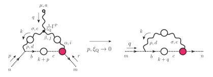
Figure 2: The unique contribution to the $(\widetilde{b})$ diagram of Fig. 1 which is non-vanishing in the $p\to 0$ limit.

These observations are particularly relevant when evaluating diagram $(\widetilde{b})$ of Fig. 1, because, unlike its counterpart $(b)$, it does not vanish in the limit $p\to 0$. The easiest way to appreciate this fact it to remember that the vanishing of graph $(b)$ relies on the fact that the term $(k+p)_{\rho}$ originating from the tree-level ghost-gluon vertex is contracted with an adjacent $\Delta^{\rho\sigma}(k)$ in the Landau gauge, see Eq. (27). However, if the $\Delta^{\rho\sigma}$ enters, in its other end, into a tree-level vertex $\widetilde{\Gamma}^{(0)}$, the longitudinal momentum $(k+p)_{\sigma}$ present in $\Gamma^{\scriptscriptstyle\mathrm{P}}$ will act on it; thus, the original $(k+p)_{\rho}$ will be contracted with $(k+p)^{\rho}/(k+p)^{2}$ instead, and will therefore survive when the limit $p\to 0$ is taken.

It turns out that there is only one possible structure of this type contained in $(\widetilde{b})$, which is shown diagrammatically in Fig. 2; then, it is relatively straightforward to establish that, in the $p\to 0$ limit, we have that

$$(\widetilde{b})_{\mu}=\frac{1}{2}q_{\mu}\Sigma(q^{2}),$$ (43)

with the 1/2 factor originating from the use of the identity $f^{ads}f^{msb}f^{nbd}=\frac{1}{2}C_{A}f^{amn}$.

Finally, one needs to consider the additional diagram $(\widetilde{c})$ which appears due to the presence of the PT-BFM special vertex $BQc{\bar{c}}$

$$\Gamma^{(0)}_{c^{n}B^{a}_{\mu}Q^{b}_{\nu}\bar{c}^{m}}(p,q,t,r)=-ig^{2}g_{\mu\nu}f^{mae}f^{ebn}.$$ (44)

In the $p\to 0$ limit then one obtains for this diagram

$$(\widetilde{c})_{\mu}=\frac{1}{2}q_{\mu}\Sigma(q^{2}),$$ (45)

which, when added to the previous result, gives for the $\widetilde{\Gamma}_{\mu}$ SDE in the $p\to 0$ limit

$$\widetilde{\Gamma}_{\mu}(q,-q,0)=q_{\mu}[1+\Sigma(q^{2})]=q_{\mu}F^{-1}(q^{2}),$$ (46)

where Eq. (39) has been used.

III.4 Derivation from the BQI

Finally, let us consider the BQI that relates the conventional and background ghost-gluon vertices, which reads Binosi and Papavassiliou (2008b)

$$\widetilde{\Gamma}_{\mu}(q,r,p) =\left\{[1+G(q^{2})]g_{\mu}^{\nu}+\frac{q_{\mu}q^{\nu}}{q^{2}}L(q^{2})\right\}{\Gamma}_{\nu}(q,r,p)+F^{-1}(p^{2})p^{\nu}K_{\mu\nu}(q,p,r)$$

$$-r^{2}F^{-1}(r^{2})K_{\mu}(q,p,r),$$ (47)

where $K_{\mu\nu}$ and $K_{\mu}$ are the auxiliary Green’s functions shown in Fig. 3, which involve composite operators appearing as a consequence of the anti-BRST symmetry present when quantizing the theory within the BFM framework Binosi and Quadri (2013).

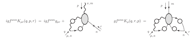
Figure 3: The auxiliary functions appearing in the ghost-gluon vertex BQI.

When taking the $p\to 0$ limit, on the one hand the second term on the right-hand side (r.h.s.) of the BQI (47) vanishes directly due to the presence of $p^{\nu}$; on the other hand, the last term vanishes in the Landau gauge, because the relation $(k+p)_{\rho}\Delta^{\rho\sigma}(k)=p_{\rho}\Delta^{\rho\sigma}(k)$ will be triggered once again. Thus, in this limit, the BQI reduces to

$$\widetilde{\Gamma}_{\mu}(q,-q,0)=\left\{[1+G(q^{2})]g_{\mu}^{\nu}+\frac{q_{\mu}q^{\nu}}{q^{2}}L(q^{2})\right\}{\Gamma}_{\nu}(q,-q,0).$$ (48)

Now, Taylor’s theorem for the conventional vertex implies ${\Gamma}_{\nu}(q,-q,0)=q_{\nu}$, so that one arrives at

$$\widetilde{\Gamma}_{\mu}(q,-q,0)=\left[1+G(q^{2})+L(q^{2})\right]q_{\mu}\,.$$ (49)

At this point, use of the Landau gauge relation Grassi et al. (2004); Aguilar et al. (2009)

$$F^{-1}(q^{2})=1+G(q^{2})+L(q^{2}),$$ (50)

together with Eq. (34), leads immediately to the result of Eq. (38).

IV A closer look at the pole part of the ghost vertex

It is well understood that, in order for the gluon mass generation to go through in the way described in Aguilar et al. (2012); Ibañez and Papavassiliou (2013); Aguilar et al. (2016), the STIs satisfied by the fundamental vertices must be realized in part by means of a longitudinally coupled pole term. This fact, in turn, imposes general restrictions on the structure of the form factors of these vertices; in this section we will study this issue for the case of the $Bc\bar{c}$ vertex $\widetilde{\Gamma}_{\mu}$, which, due to its reduced tensorial content, is particularly instructive. In the first subsection we examine in some detail the structure of the pole part of $\widetilde{\Gamma}_{\mu}$, its relation with the other form factors, together with the restrictions imposed by Taylor’s theorem. Then, in the second subsection, we introduce a concrete Ansatz for the pole part, which, in conjunction with the solution obtained from the BSE system in Sec. VI, allows for the sequential determination of all relevant pieces of $\widetilde{\Gamma}_{\mu}$.

IV.1 General considerations and alternative formulation

We start by considering the general form of the vertex $\widetilde{\Gamma}_{\mu}(q,r,p)$, given by

$${\widetilde{\Gamma}}_{\mu}(q,r,p) ={\widetilde{A}}^{\rm np}(q,r,p)q_{\mu}+{\widetilde{B}}^{\rm np}(q,r,p)p_{\mu}+\frac{q_{\mu}}{q^{2}}\widetilde{C}_{\mathrm{gh}}(q,r,p),$$ (51)

where both ${\widetilde{A}}^{\rm np}$ and ${\widetilde{B}^{\rm np}}$ are finite functions for all possible momenta $q$, $r$, and $p$. If we now take the limit $p\to 0$ on the r.h.s. of Eq. (51) and use Taylor’s theorem, we conclude that ${\widetilde{A}}^{\rm np}(q,-q,0)$ and $\widetilde{C}_{\mathrm{gh}}(q,-q,0)$ must satisfy the constraint

$$\widetilde{C}_{\mathrm{gh}}(q,-q,0)+q^{2}{\widetilde{A}}^{\rm np}(q,-q,0)=q^{2}F^{-1}(q^{2}).$$ (52)

Note that, since $F^{-1}(q^{2})$ and ${\widetilde{A}}^{\rm np}(q,-q,0)$ are finite at the origin, Eq. (52) implies that $\widetilde{C}_{\mathrm{gh}}(0,0,0)=0$ [this last result may be obtained also from by setting $r=0$ directly in the condition (16)].

Let us now introduce

$${\cal R}(q,r,p):=i\frac{D^{-1}(r^{2})-D^{-1}(p^{2})}{r^{2}-p^{2}}=\frac{r^{2}F^{-1}(r^{2})-p^{2}F^{-1}(p^{2})}{r^{2}-p^{2}},$$ (53)

and, without loss of generality, set

$${\widetilde{A}}^{\rm np}(q,r,p) ={\cal R}(q,r,p)+f_{{\scriptscriptstyle A}}(q,r,p),$$

$${\widetilde{B}^{\rm np}}(q,r,p) =2\,{\cal R}(q,r,p)+f_{{\scriptscriptstyle B}}(q,r,p),$$ (54)

where $f_{{\scriptscriptstyle A}}$ and $f_{{\scriptscriptstyle B}}$ are arbitrary, purely non-perturbative functions, assumed to be well-behaved in the entire range of their arguments, and in particular in the important limits $q\to 0$ and $p\to 0$. Note that the tree-level values for ${\widetilde{A}}^{\rm np}$ and ${\widetilde{B}}^{\rm np}$ are correctly recovered, since ${\cal R}^{(0)}=1$.

Evidently, Eq. (53) implies ${\cal R}(q,-q,0)=F^{-1}(q^{2})$; therefore

$${\widetilde{A}}^{\rm np}(q,-q,0)=F^{-1}(q^{2})+f_{{\scriptscriptstyle A}}(q,-q,0),$$ (55)

and from Eq. (52) we must have that

$$\widetilde{C}_{\mathrm{gh}}(q,-q,0)=-q^{2}f_{{\scriptscriptstyle A}}(q,-q,0).$$ (56)

Let us next contract $\widetilde{\Gamma}_{\mu}(q,r,p)$ by $q^{\mu}$; clearly, the terms proportional to ${\cal R}(q,p,r)$ saturate the STI, and thus we must have

$$q^{2}f_{{\scriptscriptstyle A}}(q,r,p)+(p\!\cdot\!q)f_{{\scriptscriptstyle B}}(q,r,p)+\widetilde{C}_{\mathrm{gh}}(q,r,p)=0.$$ (57)

Note that, in the limit $p\to 0$, Eq. (57) simply reproduces Eq. (56); however, if we take instead the limit $q\to 0$, the matching of the linear terms in $q$ yields the additional relation

$$f_{{\scriptscriptstyle B}}(0,r,-r)=2\widetilde{C}_{\mathrm{gh}}^{\prime}(r^{2}).$$ (58)

This relation is particularly interesting because it connects explicitly the term $\widetilde{C}_{\mathrm{gh}}^{\prime}(r^{2})$ that accompanies the massless pole (and enters eventually in the “mass” equation (19)) with the function $f_{{\scriptscriptstyle B}}$, which quantifies the necessary deviation of ${\widetilde{B}^{\rm np}}(q,r,p)$ from the expression that would saturate the STI identically. At this point one may verify immediately that, as first stated in Aguilar et al. (2016) (see Eq. (7.4) there),

$${\widetilde{B}^{\rm np}}(0,r,-r)=2\left[i\frac{\partial{D}^{-1}(r^{2})}{\partial r^{2}}+\widetilde{C}_{\mathrm{gh}}^{\prime}(r^{2})\right].$$ (59)

It is evident from the above considerations, and particularly from Eq. (58), that the terms of $\widetilde{\Gamma}_{\mu}(q,r,p)$ that involve $f_{{\scriptscriptstyle A}}$, $f_{{\scriptscriptstyle B}}$, and $\widetilde{C}_{\mathrm{gh}}$ must organize themselves into a transverse structure. To see this explicitly, use Eq. (57) to eliminate any of the $\widetilde{C}_{\mathrm{gh}}$, $f_{{\scriptscriptstyle A}}$ and $f_{{\scriptscriptstyle B}}$ in favor of the other two, and substitute into Eq. (51), to obtain

$${\widetilde{\Gamma}}_{\mu}(q,r,p)=(2p+q)_{\mu}{\cal R}(q,r,p)+f_{{\scriptscriptstyle B}}(q,r,p)\,p^{\sigma}P_{\sigma\mu}(q).$$ (60)

Clearly, the expression on the r.h.s. of Eq. (60) yields directly the correct Taylor limit. Note also that $q^{2}p^{\sigma}P_{\sigma\mu}(q)=(p\!\cdot\!q)\,r_{\mu}-(r\!\cdot\!q)\,p_{\mu}$, the latter being the transverse vector introduced by Ball and Chiu Ball and Chiu (1980).

According to Eq. (60), all memory of the longitudinally coupled pole has been transferred to the transverse part of the vertex. Of course, this simple reorganization of terms leading to Eq. (60) could not possibly induce any modifications to the contribution of the ghost loops to $\Delta^{-1}(0)$. To see that this is indeed so, note that the first term of Eq. (60), in the limit $q\to 0$, triggers the “seagull identity” and cancels exactly against the seagull diagram, while the second term gives a contribution that is manifestly transverse ($p\to k$),

$$P_{\mu\nu}(q)\widetilde{\Pi}(q^{2})=g^{2}C_{A}P_{\sigma\nu}(q)\int_{k}k_{\mu}k^{\sigma}D(k)D(k-q)f_{{\scriptscriptstyle B}}(q,k-q,-k).$$ (61)

Then, as $q\to 0$, we obtain

$$\widetilde{\Pi}(0)=\frac{g^{2}C_{A}}{d}\int_{k}k^{2}D^{2}(k)f_{{\scriptscriptstyle B}}(0,k,-k),$$ (62)

which, after taking into account Eq. (58), coincides with Eq. (6.11) of Aguilar et al. (2016) (see also Eq. (7.3) of the same paper).

Let us point out that the ${\widetilde{\Gamma}}_{\mu}$ of Eq. (60) could have been supplemented from the beginning by a transverse piece, whose form factor, unlike that of Eq. (60), would vanish as $q\to 0$; this is indeed the construction of Ball and Chiu (1980), where a term $a(q,r,p)\left[(r\!\cdot\!q)\,p_{\mu}-(p\!\cdot\!q)\,r_{\mu})\right]$ is included, with $a(q,r,p)$ finite. In the present context, the effect of including this additional term would be to modify $f_{{\scriptscriptstyle B}}\to f_{{\scriptscriptstyle B}}+q^{2}a$; this extra term is clearly irrelevant as far as the gluon mass generation is concerned; for instance, it would have a vanishing contribution to the r.h.s. of Eq. (62). Therefore, $a(q,r,p)$ will be neglected in what follows.

IV.2 A special case

Let us now consider a special realization of the general scenario presented above, which admits a complete solution. Specifically, we set

$$f_{{\scriptscriptstyle A}}(q,r,p)=f(q,r,p)=\frac{1}{2}f_{{\scriptscriptstyle B}}(q,r,p),$$ (63)

which, using Eq. (57), implies

$$f(q,r,p)=-\frac{\widetilde{C}_{\mathrm{gh}}(q,r,p)}{r^{2}-p^{2}}.$$ (64)

Next, for $\widetilde{C}_{\mathrm{gh}}$ we employ, similarly to what we were lead to in Eq. (21) for the gluon case, the simple Ansatz

$$\widetilde{C}_{\mathrm{gh}}(q,r,p)=r^{2}h(r^{2})-p^{2}h(p^{2}),$$ (65)

which clearly satisfies the condition $\widetilde{C}_{\mathrm{gh}}(0,r,-r)=0$, as required on general grounds. In addition, the quantity $\widetilde{C}_{\mathrm{gh}}^{\prime}(r^{2})$ is now given by

$$\widetilde{C}_{\mathrm{gh}}^{\prime}(r^{2})=[r^{2}h(r^{2})]^{\prime},$$ (66)

while, in the Taylor limit,

$$\widetilde{C}_{\mathrm{gh}}(q,-q,0)=q^{2}h(q^{2})=-q^{2}f(q,-q,0),$$ (67)

exactly as required from Eq. (56).

The above Ansatz allows for a complete solution of the part of the ghost sector that affects the dynamics of the gluon mass generation, because, once $\widetilde{C}_{\mathrm{gh}}^{\prime}(r^{2})$ has been determined from the corresponding BSE system, all other quantities may be deduced from Eq. (54) together with Eq. (63) through (66).

In particular,

$$r^{2}h(r^{2})=c+\int_{0}^{r^{2}}\!{\rm d}y\,\widetilde{C}_{\mathrm{gh}}^{\prime}(y)$$ (68)

where $c$ is the integration constant. Evidently, $c$ drops out when forming $\widetilde{C}_{\mathrm{gh}}(q,r,p)$ using Eq. (66),

$$\widetilde{C}_{\mathrm{gh}}(q,r,p)=\int_{0}^{r^{2}}\!{\rm d}y\,\widetilde{C}_{\mathrm{gh}}^{\prime}(y)-\int_{0}^{p^{2}}{\rm d}y\,\widetilde{C}_{\mathrm{gh}}^{\prime}(y);$$ (69)

on the other hand, in the Taylor limit ($p\to 0$) Eq. (69) yields

$$\widetilde{C}_{\mathrm{gh}}(q,-q,0)=\int_{0}^{q^{2}}dy\,\widetilde{C}_{\mathrm{gh}}^{\prime}(y),$$ (70)

which may be reconciled with Eq. (67) and Eq. (68) only for the value $c=0$.

At this point it is natural to introduce the combination

$$F_{{\rm eff}}^{-1}(q^{2}) :=F^{-1}(q^{2})+h(q^{2})$$

$$=F^{-1}(q^{2})[1+\underbrace{h(q^{2})F(q^{2})}_{\delta(q^{2})}],$$ (71)

where the function

$$\delta(q^{2})=D(q^{2})\int_{0}^{q^{2}}dy\,\widetilde{C}_{\mathrm{gh}}^{\prime}(y)$$ (72)

quantifies the relative deviation of the vertex form factors from their “canonical” form, due to the presence of the pole term. Specifically, one obtains

$${\widetilde{A}}^{\rm np}(q,r,p)={\cal R}_{{\rm eff}}(q,r,p)=\frac{1}{2}{\widetilde{B}^{\rm np}}(q,r,p)\,,$$ (73)

where ${\cal R}_{{\rm eff}}$ is obtained from the ${\cal R}$ in Eq. (53) by carrying out the substitution $F^{-1}(q^{2})\to F_{{\rm eff}}^{-1}(q^{2})$.

V Coupled Dynamics of massless pole formation

The actual behavior of $\widetilde{C}_{\mathrm{gl}}^{\prime}$ and $\widetilde{C}_{\mathrm{gh}}^{\prime}$ is determined by a homogeneous system of linear integral equations, which may be derived from the SDEs satisfied by the corresponding $BQ^{2}$ and $Bc\bar{c}$ vertices as $q\to 0$ Aguilar et al. (2012, 2017). As in this limit the zeroth order terms vanish by virtue of Eq. (16), the derivative terms become the leading contributions, and the resulting homogeneous equations assume the form of two coupled BSEs, given by

$$f^{amn}\lim_{q\to 0}\widetilde{C}_{\alpha\beta}(q,r,p)=f^{abc}\lim_{q\to 0}\Bigg{\{} \int_{k}\widetilde{C}_{\gamma\delta}(q,k,-k-q)\Delta^{\gamma\rho}(k)\Delta^{\delta\sigma}(k+q){\cal K}_{1\rho\alpha\beta\sigma}^{bmnc}(-k,r,p,k+q)$$

$$+ \int_{k}\widetilde{C}_{\mathrm{gh}}(q,k,-k-q)D(k)D(k+q){\cal K}_{2\alpha\beta}^{bmnc}(-k,r,p,k+q)\Bigg{\}},$$

$$f^{amn}\lim_{q\to 0}\widetilde{C}_{\mathrm{gh}}(q,r,p)=f^{abc}\lim_{q\to 0}\Bigg{\{} \int_{k}\widetilde{C}_{\gamma\delta}(q,k,-k-q)\Delta^{\gamma\rho}(k)\Delta^{\delta\sigma}(k+q){\cal K}_{3\rho\sigma}^{bmnc}(-k,r,p,k+q)$$

$$+ \int_{k}\widetilde{C}_{\mathrm{gh}}(q,k,-k-q)D(k)D(k+q){\cal K}_{4}^{bmnc}(-k,r,p,k+q)\Bigg{\}}.$$

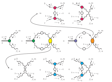
Figure 4: The BSE satisfied by the gluon bound-state wave function $\widetilde{C}_{\alpha\beta}$ (center) in the presence of both gluon and ghost massless poles. The simplified four-gluon and gluon-ghost kernels used are also shown.

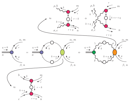
Figure 5: The BSE satisfied by the ghost bound-state wave function $\widetilde{C}_{\mathrm{gh}}$ (center) in the presence of both gluon and ghost massless poles. The simplified four-ghost and gluon-ghost kernels used are also shown.

To proceed further, we will approximate the four-point BS kernels ${\mathcal{K}}_{i}$ by their lowest-order set of diagrams shown in Fig. 4 and Fig. 5, in which the various diagrams contain fully dressed propagators and vertices (notice that all gluon propagators are “quantum” ones, and all vertices of the “ $\Gamma$ type”). In particular for the three-gluon and ghost-gluon vertices we will consider the simple Ansätze

$$\Gamma_{\mu\alpha\beta}(q,r,p)=f_{\mathrm{gl}}(r)\Gamma^{(0)}_{\mu\alpha\beta}(q,r,p),$$

$$\Gamma_{\mu}(q,r,p)=f_{\mathrm{gh}}(r)\Gamma^{(0)}_{\mu}(q,r,p),$$ (75)

where $\Gamma^{(0)}$ represents the standard tree-level expression of the corresponding vertex, and the form factors $f_{\mathrm{gl}}$ and $f_{\mathrm{gh}}$ are considered to be functions of a single kinematic variable. We then arrive at the following final equations

$$\widetilde{C}_{\mathrm{gl}}^{\prime}(q^{2}) =\frac{8\pi}{3}\alpha_{s}C_{A}\!\left[\int_{k}\!\widetilde{C}_{\mathrm{gl}}^{\prime}(k^{2})\Delta^{2}(k)\Delta(k+q){\cal N}_{1}(k,q)+\frac{1}{4}\int_{k}\!\widetilde{C}_{\mathrm{gh}}^{\prime}(k^{2})D^{2}(k)D(k+q){\cal N}_{2}(k,q)\!\right]\!,$$

$$\widetilde{C}_{\mathrm{gh}}^{\prime}(q^{2}) =2\pi\alpha_{s}C_{A}\!\left[\int_{k}\!\widetilde{C}_{\mathrm{gl}}^{\prime}(k^{2})\Delta^{2}(k)D(k+q){\cal N}_{3}(k,q)+\frac{1}{2}\int_{k}\!\widetilde{C}_{\mathrm{gh}}^{\prime}(k^{2})D^{2}(k)\Delta(k+q){\cal N}_{4}(k,q)\!\right]\!,$$ (76)

where

$${\cal N}_{1}(k,q) =\frac{(q\!\cdot\!k)[q^{2}k^{2}-(q\!\cdot\!k)^{2}]}{q^{4}k^{2}(k+q)^{2}}f_{\mathrm{gl}}^{2}(k+q)\left[8q^{2}k^{2}+6(q\!\cdot\!k)(q^{2}+k^{2})+3(q^{4}+k^{4})+(q\!\cdot\!k)^{2}\right],$$

$${\cal N}_{2}(k,q) =\frac{(q\!\cdot\!k)[q^{2}k^{2}-(q\!\cdot\!k)^{2}]}{q^{4}}f_{\mathrm{gh}}^{2}(k+q),$$

$${\cal N}_{3}(k,q) =\frac{(q\!\cdot\!k)[q^{2}k^{2}-(q\!\cdot\!k)^{2}]}{q^{2}k^{2}}f_{\mathrm{gh}}^{2}(k+q),$$

$${\cal N}_{4}(k,q) =\frac{(q\!\cdot\!k)[q^{2}k^{2}-(q\!\cdot\!k)^{2}]}{q^{2}(k+q)^{2}}f_{\mathrm{gh}}^{2}(k+q).$$ (77)

Notice, in particular, that in the $q\to 0$ limit, $\widetilde{C}_{\mathrm{gl}}(0)$ saturates to a constant Binosi and Papavassiliou (2017), whereas the structure of the ${\cal N}_{3}$ and ${\cal N}_{4}$ kernels implies that $\widetilde{C}_{\mathrm{gh}}(0)=0$.

   

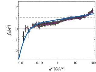
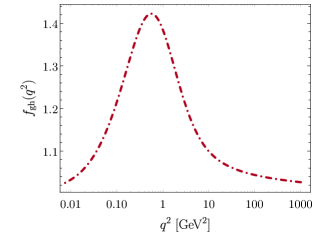
Figure 6: (Left panel) SU(3) lattice data (evaluated with various $\beta$, volumes and lattice actions) for the form factor $f_{\mathrm{gl}}$ in the symmetric configuration Athenodorou et al. (2016); Boucaud et al. (2017); the continuous line corresponds to the optimal data description obtained in Binosi and Papavassiliou (2017) when solving the BSE in the absence of ghosts. (Right panel) The ghost-gluon vertex form factor $f_{\mathrm{gh}}$ in the symmetric configuration obtained from solving its SDE.

VI Numerical Analysis

Before proceeding to solve the BSE system (76), some of the functions that appears in it ought to be specified.

To begin with, for the gluon propagator $\Delta$ and ghost dressing function $F$ we will employ the available SU(3) lattice data Bogolubsky et al. (2009). As for the vertex form factors $f_{\mathrm{gl}}$ and $f_{\mathrm{gh}}$, we use the curves shown in Fig. 6. More specifically, in the case of the three-gluon vertex, the left panel of Fig. 6 shows a compilation of the lattice data of this form factor in the symmetric configuration (defined as $q^{2}=p^{2}=r^{2}$ and $q\!\cdot\!p=q\!\cdot\!r=p\!\cdot\!r=-q^{2}/2$, e.g., with a $2\pi/3$ angle between each pair of momenta) Athenodorou et al. (2016); Boucaud et al. (2017), properly normalized by dividing out the coupling [$g=2$ at $\mu=4.3$ GeV for the data set at hand, corresponding to $\alpha_{s}=0.32$]. Notice, in particular, the suppression of the vertex with respect to its tree-level value, as well as the sign reversal (the so-called “zero crossing”) at small momenta, followed by a (logarithmic) divergence at the origin. This characteristic behavior can be traced back to the delicate balance between contributions originating from gluon loops, which are “protected” by the corresponding gluon mass, and the “unprotected” logarithms coming from the ghost loops that contain (even nonperturbatively) massless ghosts Alkofer et al. (2009); Tissier and Wschebor (2011); Pelaez et al. (2013); Aguilar et al. (2014a); Blum et al. (2014); Eichmann et al. (2014); Williams et al. (2016); Cyrol et al. (2016).

   

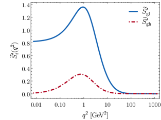
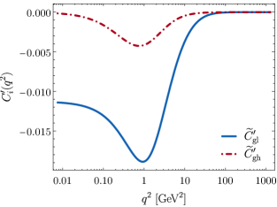
Figure 7: Unnormalized gluon and ghost solutions $\widetilde{S}_{\mathrm{gl}}^{\prime}$ and $\widetilde{S}_{\mathrm{gh}}^{\prime}$ of the BSE system (76) (left panel), and the corresponding normalized curves (right panel).

For the ghost-gluon vertex, instead, the right panel of Fig. 6 shows the numerical solution of the corresponding vertex SDE equation in the symmetric configuration within the so-called “one-loop dressed” approximation. The form factor is found to be equal at its tree-level value at both IR and UV values, with a characteristic peak appearing at intermediate momenta (around 0.75 GeV). The presence of this peak is in fact quite general, appearing in different kinematic configurations, e.g., the soft gluon ($q\to 0$) and soft ghost ($p\to 0$) limits (see respectively Fig. 6 and 7 of Ref. Aguilar et al. (2013)).

The (unnormalized) solutions $\widetilde{S}_{\mathrm{gl}}^{\prime}$ and $\widetilde{S}_{\mathrm{gh}}^{\prime}$ obtained when using these ingredients in the BSE system (76) corresponds to the eigenvalue $\alpha_{s}^{\scriptscriptstyle\mathrm{BSE}}=0.43$, and are shown on the left panel of Fig. 7. While it is clear that QCD dynamics is strong enough to generate massless poles for both vertices studied, the presence of a hierarchy in their relative “strengths” is also evident, as $\widetilde{S}_{\mathrm{gh}}^{\prime}$ is considerably suppressed with respect to $\widetilde{S}_{\mathrm{gl}}^{\prime}$ (with the latter being roughly 5 times the former at peak value).

The common normalization constant $c$ can be determined with the procedure recently described in Binosi and Papavassiliou (2017), that is by requiring that the normalized gluon BS amplitude give rise, when plugged into Eq. (23), to a running gluon mass that is $(i)$ monotonically decreasing and $(ii)$ vanishes in the UV. This implies Binosi and Papavassiliou (2017) $C_{i}^{\prime}=-|c|S_{i}^{\prime}$, with

$$|c|=\frac{\Delta^{-1}(0)}{\displaystyle\int_{0}^{\infty}\!{\rm d}y\,\widetilde{S}_{\mathrm{gl}}^{\prime}(y)},$$ (78)

and, correspondingly,

$$m^{2}(q^{2})=-\int_{q^{2}}^{\infty}\!\!{\rm d}y\,\widetilde{C}_{\mathrm{gl}}^{\prime}(y).$$ (79)

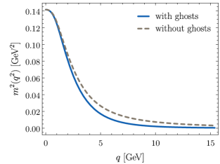
Figure 8: The gluon mass obtained by integrating the gluon BSE solution, compared to the one obtained in the absence of ghosts.

The resulting gluon mass is shown in Fig. 8, where it is also compared to the result obtained in Binosi and Papavassiliou (2017) in the absence of ghosts, when $\alpha_{s}^{\scriptscriptstyle\mathrm{BSE}}=0.45$. As can be clearly appreciated, the presence of ghosts implies a faster running; indeed, one finds that the mass can be accurately fitted through the formula Aguilar et al. (2014b)

$$m^{2}(q^{2})=m^{2}(0)/[1+(q^{2}/m_{1}^{2})^{1+p}],$$ (80)

with $m_{1}=0.37$ GeV and $p=0.24$ as opposed to $m_{1}=0.36$ GeV and $p=0.1$ in the absence of ghosts. An additional consistency check can be performed by substituting Eq. (78) into Eq. (19), thus obtaining a second order algebraic equation for $\alpha_{s}$, given by

$$A\alpha_{s}^{2}+B\alpha_{s}+C=0,$$ (81)

where

$$A =\frac{3C^{2}_{A}}{32\pi^{3}}F(0)\int_{0}^{\infty}{\rm d}y\,y^{2}{\Delta}^{2}(y)Y(y)\widetilde{S}_{\mathrm{gl}}^{\prime}(y),$$

$$B =-\frac{3C_{A}}{8\pi}F(0)\int_{0}^{\infty}{\rm d}y\,\left[y^{2}{\Delta}^{2}(y)\widetilde{S}_{\mathrm{gl}}^{\prime}(y)-\frac{1}{3}y^{2}D^{2}(y^{2})\widetilde{S}_{\mathrm{gh}}^{\prime}(y)\right],$$

$$C =-\int_{0}^{\infty}{\rm d}y\,\widetilde{S}_{\mathrm{gl}}^{\prime}(y).$$ (82)

Substituting into Eq. (82) the solutions found for $\widetilde{S}_{\mathrm{gl}}^{\prime}(y)$ and $\widetilde{S}_{\mathrm{gh}}^{\prime}(y)$ we obtain (all values in GeV²) $A=110.02$, $B=-24.25$, $C=-9.32$, yielding $\alpha_{s}^{\scriptscriptstyle\mathrm{SDE}}=0.43\equiv\alpha_{s}^{\scriptscriptstyle\mathrm{BSE}}$.

   

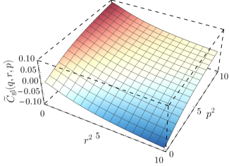
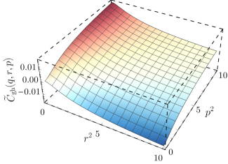
Figure 9: Reconstructed form factors $\widetilde{C}_{\mathrm{gl}}$ and $\widetilde{C}_{\mathrm{gh}}$ of the pole parts of the three-gluon and gluon-ghost vertices. The momenta $p$ and $r$ are treated as independent.

As a final step we can fully reconstruct the form factors characterizing the three-gluon and ghost-gluon vertices pole parts, by using the results obtained so far in conjunction with Eqs. (22) and (65). The results are shown in Fig. 9; notice that due to their suppression, the presence of $\widetilde{C}_{\mathrm{gl}}$ and $\widetilde{C}_{\mathrm{gh}}$ will not appreciably modify the no-pole parts. This can be seen also in Fig. 10 where we plot the quantity $\delta(q^{2})$ introduced in Eq. (72), which quantifies the relative deviation of the gluon-ghost vertex form factors from their “canonical” form, due to the presence of the pole term. Such deviation saturates at the 2% level, making the presence of poles practically undetectable from studies of three-point form factors alone.

VII Conclusions

In this work we have studied the impact of the ghost sector on the dynamics of gluon mass generation, using the specific framework provided by the PT-BFM formalism. In this approach, the infrared finiteness of the gluon propagator, and the gluon mass connected to it, arise from the action of massless bound state poles, which enter in the structure of the fundamental vertices of the theory. Within this context, our present analysis reveals that the contribution of the poles associated with the ghost gluon vertex $\widetilde{\Gamma}_{\mu}$ are particularly suppressed with respect to those originating from the corresponding poles of $\widetilde{\Gamma}_{\mu\alpha\beta}$. This fact is illustrated rather clearly in Fig. 9, where both vertex functions, $\widetilde{C}_{\mathrm{gl}}(q,r,p)$ and $\widetilde{C}_{\mathrm{gh}}(q,r,p)$, which accompany the corresponding poles and account for their relative “strengths”, are directly compared, for the entire range of Euclidean momenta. Evidently, whereas the qualitative structure of both is rather similar, their relative size is substantially different. Consequently, the “gluonic” pole contributions, $\widetilde{C}_{\mathrm{gl}}(q,r,p)$, are completely decisive both for the generation and the momentum evolution of the gluon mass. The above result is non-trivial, in the sense that there is no obvious a-priori argument that would imply the observed suppression of the ghost sector. In fact, the mere existence of solutions of the BSE system, let alone the observed insensitivity of the relevant eigenvalue to the presence of $\widetilde{C}_{\mathrm{gh}}^{\prime}(r^{2})$, may be only established once the full analysis has been carried out.

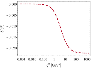
Figure 10: The function $\delta$ measuring the relative deviation of the gluon-ghost vertex form factors from their “canonical” form, due to the presence of the pole term.

We emphasize that throughout our analysis we have explicitly neglected any possible effects stemming from poles associated with the four-gluon vertex. In that sense, all such possible terms have been assumed to vanish, or be numerically suppressed. It would be clearly interesting to eventually relax this assumption and gain some direct information of the actual size of such contributions. Note, however, that from the technical point of view this task is particularly complex, mainly due to the rich tensorial structure of this vertex Pascual and Tarrach (1980); Binosi et al. (2014); Cyrol et al. (2015); Gracey (2017). In fact, in this case the corresponding vertex functions, $\widetilde{C}_{\scriptscriptstyle\mathrm{4gl}}(q,r,p,t)$, depend on four rather than three kinematic variables, and, equivalently, their derivatives as $q\to 0$ will depend on two instead of one, which will vastly complicate the structure and treatment of the would-be BSE system.

Let us finally mention that an additional novel element presented in the present work is the analysis of the behavior of $\widetilde{\Gamma}_{\mu}$ in the limit of vanishing ghost momentum, leading to the derivation of the analogue of Taylor’s theorem for the PT-BFM formalism. The resulting constraint relates one of the form factor of $\widetilde{\Gamma}_{\mu}$ with the ghost-dressing function. In addition to its relevance for the reconstruction of the full $\widetilde{C}_{\mathrm{gh}}(q,r,p)$ presented here, this particular constraint might turn useful for future lattice simulations of the PT-BFM vertices Binosi and Quadri (2012); Cucchieri and Mendes (2012), which could provide further valuable insights to this entire field of research.

References

- Cloet and Roberts (2014) I. C. Cloet and C. D. Roberts, Prog. Part. Nucl. Phys. 77, 1 (2014), arXiv:1310.2651 [nucl-th] .
- Roberts (2017) C. D. Roberts, Few Body Syst. 58, 5 (2017), arXiv:1606.03909 [nucl-th] .
- Roberts and Mezrag (2017) C. D. Roberts and C. Mezrag, Proceedings, 12th Conference on Quark Confinement and the Hadron Spectrum (Confinement XII): Thessaloniki, Greece, EPJ Web Conf. 137, 01017 (2017), arXiv:1611.09863 [nucl-th] .
- Aguilar and Papavassiliou (2006) A. C. Aguilar and J. Papavassiliou, JHEP 12, 012 (2006), hep-ph/0610040 .
- Aguilar et al. (2008) A. C. Aguilar, D. Binosi, and J. Papavassiliou, Phys. Rev. D78, 025010 (2008), arXiv:0802.1870 [hep-ph] .
- Aguilar et al. (2012) A. Aguilar, D. Ibanez, V. Mathieu, and J. Papavassiliou, Phys. Rev. D85, 014018 (2012), arXiv:1110.2633 [hep-ph] .
- Ibañez and Papavassiliou (2013) D. Ibañez and J. Papavassiliou, Phys. Rev. D87, 034008 (2013), arXiv:1211.5314 [hep-ph] .
- Aguilar et al. (2016) A. C. Aguilar, D. Binosi, C. T. Figueiredo, and J. Papavassiliou, Phys. Rev. D94, 045002 (2016), arXiv:1604.08456 [hep-ph] .
- Cornwall (1982) J. M. Cornwall, Phys. Rev. D26, 1453 (1982).
- Cucchieri and Mendes (2007) A. Cucchieri and T. Mendes, PoS LAT2007, 297 (2007), arXiv:0710.0412 [hep-lat] .
- Cucchieri and Mendes (2008) A. Cucchieri and T. Mendes, Phys. Rev. Lett. 100, 241601 (2008), arXiv:0712.3517 [hep-lat] .
- Cucchieri and Mendes (2010) A. Cucchieri and T. Mendes, Phys. Rev. D81, 016005 (2010), arXiv:0904.4033 [hep-lat] .
- Bowman et al. (2007) P. O. Bowman et al., Phys. Rev. D76, 094505 (2007), hep-lat/0703022 .
- Bogolubsky et al. (2009) I. Bogolubsky, E. Ilgenfritz, M. Muller-Preussker, and A. Sternbeck, Phys. Lett. B676, 69 (2009), arXiv:0901.0736 [hep-lat] .
- Oliveira and Silva (2009) O. Oliveira and P. Silva, PoS LAT2009, 226 (2009), arXiv:0910.2897 [hep-lat] .
- Ayala et al. (2012) A. Ayala, A. Bashir, D. Binosi, M. Cristoforetti, and J. Rodriguez-Quintero, Phys. Rev. D86, 074512 (2012), arXiv:1208.0795 [hep-ph] .
- Bicudo et al. (2015) P. Bicudo, D. Binosi, N. Cardoso, O. Oliveira, and P. J. Silva, Phys. Rev. D92, 114514 (2015), arXiv:1505.05897 [hep-lat] .
- Lavelle (1991) M. Lavelle, Phys. Rev. D44, 26 (1991).
- Halzen et al. (1993) F. Halzen, G. I. Krein, and A. A. Natale, Phys. Rev. D47, 295 (1993).
- Philipsen (2002) O. Philipsen, Nucl. Phys. B628, 167 (2002), arXiv:hep-lat/0112047 [hep-lat] .
- Szczepaniak and Swanson (2002) A. P. Szczepaniak and E. S. Swanson, Phys. Rev. D65, 025012 (2002), arXiv:hep-ph/0107078 [hep-ph] .
- Aguilar and Natale (2004) A. C. Aguilar and A. A. Natale, JHEP 08, 057 (2004), hep-ph/0408254 .
- Kondo (2006) K.-I. Kondo, Phys. Rev. D74, 125003 (2006), hep-th/0609166 .
- Braun et al. (2010) J. Braun, H. Gies, and J. M. Pawlowski, Phys. Lett. B684, 262 (2010), arXiv:0708.2413 [hep-th] .
- Epple et al. (2008) D. Epple, H. Reinhardt, W. Schleifenbaum, and A. Szczepaniak, Phys. Rev. D77, 085007 (2008), arXiv:0712.3694 [hep-th] .
- Boucaud et al. (2008) P. Boucaud et al., JHEP 06, 099 (2008), arXiv:0803.2161 [hep-ph] .
- Dudal et al. (2008) D. Dudal, J. A. Gracey, S. P. Sorella, N. Vandersickel, and H. Verschelde, Phys. Rev. D78, 065047 (2008), arXiv:0806.4348 [hep-th] .
- Fischer et al. (2009) C. S. Fischer, A. Maas, and J. M. Pawlowski, Annals Phys. 324, 2408 (2009), arXiv:0810.1987 [hep-ph] .
- Aguilar et al. (2009) A. C. Aguilar, D. Binosi, J. Papavassiliou, and J. Rodriguez-Quintero, Phys. Rev. D80, 085018 (2009), arXiv:0906.2633 [hep-ph] .
- Rodriguez-Quintero (2011) J. Rodriguez-Quintero, JHEP 1101, 105 (2011), arXiv:1005.4598 [hep-ph] .
- Campagnari and Reinhardt (2010) D. R. Campagnari and H. Reinhardt, Phys. Rev. D82, 105021 (2010), arXiv:1009.4599 [hep-th] .
- Tissier and Wschebor (2010) M. Tissier and N. Wschebor, Phys. Rev. D82, 101701 (2010), arXiv:1004.1607 [hep-ph] .
- Kondo (2010) K.-I. Kondo, Phys. Rev. D82, 065024 (2010), arXiv:1005.0314 [hep-th] .
- Pennington and Wilson (2011) M. Pennington and D. Wilson, Phys. Rev. D84, 119901 (2011), arXiv:1109.2117 [hep-ph] .
- Watson and Reinhardt (2012) P. Watson and H. Reinhardt, Phys. Rev. D85, 025014 (2012), arXiv:1111.6078 [hep-ph] .
- Kondo (2011) K.-I. Kondo, Phys. Rev. D84, 061702 (2011), arXiv:1103.3829 [hep-th] .
- Serreau and Tissier (2012) J. Serreau and M. Tissier, Phys. Lett. B712, 97 (2012), arXiv:1202.3432 [hep-th] .
- Strauss et al. (2012) S. Strauss, C. S. Fischer, and C. Kellermann, Phys. Rev. Lett. 109, 252001 (2012), arXiv:1208.6239 [hep-ph] .
- Siringo (2014) F. Siringo, Phys. Rev. D90, 094021 (2014), arXiv:1408.5313 [hep-ph] .
- Binosi et al. (2015) D. Binosi, L. Chang, J. Papavassiliou, and C. D. Roberts, Phys. Lett. B742, 183 (2015), arXiv:1412.4782 [nucl-th] .
- Aguilar et al. (2015) A. Aguilar, D. Binosi, and J. Papavassiliou, Phys. Rev. D91, 085014 (2015), arXiv:1501.07150 [hep-ph] .
- Huber (2015) M. Q. Huber, Phys. Rev. D91, 085018 (2015), arXiv:1502.04057 [hep-ph] .
- Capri et al. (2015) M. A. L. Capri, D. Dudal, D. Fiorentini, M. S. Guimaraes, I. F. Justo, A. D. Pereira, B. W. Mintz, L. F. Palhares, R. F. Sobreiro, and S. P. Sorella, Phys. Rev. D92, 045039 (2015), arXiv:1506.06995 [hep-th] .
- Binosi et al. (2017) D. Binosi, C. Mezrag, J. Papavassiliou, C. D. Roberts, and J. Rodriguez-Quintero, Phys. Rev. D96, 054026 (2017), arXiv:1612.04835 [nucl-th] .
- Glazek et al. (2017) S. D. Glazek, M. Gómez-Rocha, J. More, and K. Serafin, Phys. Lett. B773, 172 (2017), arXiv:1705.07629 [hep-ph] .
- Gao et al. (2017) F. Gao, S.-X. Qin, C. D. Roberts, and J. Rodriguez-Quintero, (2017), arXiv:1706.04681 [hep-ph] .
- Cornwall and Papavassiliou (1989) J. M. Cornwall and J. Papavassiliou, Phys. Rev. D40, 3474 (1989).
- Pilaftsis (1997) A. Pilaftsis, Nucl. Phys. B487, 467 (1997), hep-ph/9607451 .
- Binosi and Papavassiliou (2002a) D. Binosi and J. Papavassiliou, Phys. Rev. D66, 111901(R) (2002a), hep-ph/0208189 .
- Binosi and Papavassiliou (2004) D. Binosi and J. Papavassiliou, J.Phys.G G30, 203 (2004), arXiv:hep-ph/0301096 [hep-ph] .
- Binosi and Papavassiliou (2009) D. Binosi and J. Papavassiliou, Phys. Rept. 479, 1 (2009), arXiv:0909.2536 [hep-ph] .
- Abbott (1981) L. F. Abbott, Nucl. Phys. B185, 189 (1981).
- Binosi and Papavassiliou (2008a) D. Binosi and J. Papavassiliou, Phys. Rev. D77, 061702 (2008a), arXiv:0712.2707 [hep-ph] .
- Binosi and Papavassiliou (2008b) D. Binosi and J. Papavassiliou, JHEP 0811, 063 (2008b), arXiv:0805.3994 [hep-ph] .
- Aguilar and Papavassiliou (2010) A. C. Aguilar and J. Papavassiliou, Phys. Rev. D81, 034003 (2010), arXiv:0910.4142 [hep-ph] .
- Schwinger (1962a) J. S. Schwinger, Phys. Rev. 125, 397 (1962a).
- Schwinger (1962b) J. S. Schwinger, Phys. Rev. 128, 2425 (1962b).
- Jackiw and Johnson (1973) R. Jackiw and K. Johnson, Phys. Rev. D8, 2386 (1973).
- Smit (1974) J. Smit, Phys. Rev. D10, 2473 (1974).
- Eichten and Feinberg (1974) E. Eichten and F. Feinberg, Phys. Rev. D10, 3254 (1974).
- Poggio et al. (1975) E. C. Poggio, E. Tomboulis, and S. H. H. Tye, Phys. Rev. D11, 2839 (1975).
- Binosi and Papavassiliou (2017) D. Binosi and J. Papavassiliou, (2017), arXiv:1709.09964 [hep-ph] .
- Taylor (1971) J. C. Taylor, Nucl. Phys. B33, 436 (1971).
- Binosi and Papavassiliou (2002b) D. Binosi and J. Papavassiliou, Phys. Rev. D66, 025024 (2002b), arXiv:hep-ph/0204128 [hep-ph] .
- Binosi and Quadri (2013) D. Binosi and A. Quadri, Phys. Rev. D88, 085036 (2013), arXiv:1309.1021 [hep-th] .
- Grassi et al. (2004) P. A. Grassi, T. Hurth, and A. Quadri, Phys. Rev. D70, 105014 (2004), hep-th/0405104 .
- Binosi et al. (2012) D. Binosi, D. Ibañez, and J. Papavassiliou, Phys. Rev. D86, 085033 (2012), arXiv:1208.1451 [hep-ph] .
- Aguilar et al. (2013) A. C. Aguilar, D. Ibañez, and J. Papavassiliou, Phys. Rev. D87, 114020 (2013), arXiv:1303.3609 [hep-ph] .
- Ball and Chiu (1980) J. S. Ball and T.-W. Chiu, Phys. Rev. D22, 2542 (1980).
- Aguilar et al. (2017) A. C. Aguilar, D. Binosi, and J. Papavassiliou, Phys. Rev. D95, 034017 (2017), arXiv:1611.02096 [hep-ph] .
- Athenodorou et al. (2016) A. Athenodorou, D. Binosi, P. Boucaud, F. De Soto, J. Papavassiliou, J. Rodriguez-Quintero, and S. Zafeiropoulos, Phys. Lett. B761, 444 (2016), arXiv:1607.01278 [hep-ph] .
- Boucaud et al. (2017) P. Boucaud, F. De Soto, J. Rodríguez-Quintero, and S. Zafeiropoulos, Phys. Rev. D95, 114503 (2017), arXiv:1701.07390 [hep-lat] .
- Alkofer et al. (2009) R. Alkofer, M. Q. Huber, and K. Schwenzer, Eur. Phys. J. C62, 761 (2009), arXiv:0812.4045 [hep-ph] .
- Tissier and Wschebor (2011) M. Tissier and N. Wschebor, Phys. Rev. D84, 045018 (2011), arXiv:1105.2475 [hep-th] .
- Pelaez et al. (2013) M. Pelaez, M. Tissier, and N. Wschebor, Phys. Rev. D88, 125003 (2013), arXiv:1310.2594 [hep-th] .
- Aguilar et al. (2014a) A. C. Aguilar, D. Binosi, D. Ibañez, and J. Papavassiliou, Phys. Rev. D89, 085008 (2014a), arXiv:1312.1212 [hep-ph] .
- Blum et al. (2014) A. Blum, M. Q. Huber, M. Mitter, and L. von Smekal, Phys. Rev. D89, 061703 (2014), arXiv:1401.0713 [hep-ph] .
- Eichmann et al. (2014) G. Eichmann, R. Williams, R. Alkofer, and M. Vujinovic, Phys. Rev. D89, 105014 (2014), arXiv:1402.1365 [hep-ph] .
- Williams et al. (2016) R. Williams, C. S. Fischer, and W. Heupel, Phys. Rev. D93, 034026 (2016), arXiv:1512.00455 [hep-ph] .
- Cyrol et al. (2016) A. K. Cyrol, L. Fister, M. Mitter, J. M. Pawlowski, and N. Strodthoff, Phys. Rev. D94, 054005 (2016), arXiv:1605.01856 [hep-ph] .
- Aguilar et al. (2014b) A. C. Aguilar, D. Binosi, and J. Papavassiliou, Phys. Rev. D89, 085032 (2014b), arXiv:1401.3631 [hep-ph] .
- Pascual and Tarrach (1980) P. Pascual and R. Tarrach, Nucl. Phys. B174, 123 (1980).
- Binosi et al. (2014) D. Binosi, D. Ibañez, and J. Papavassiliou, JHEP 1409, 059 (2014), arXiv:1407.3677 [hep-ph] .
- Cyrol et al. (2015) A. K. Cyrol, M. Q. Huber, and L. von Smekal, Eur. Phys. J. C75, 102 (2015), arXiv:1408.5409 [hep-ph] .
- Gracey (2017) J. A. Gracey, Phys. Rev. D95, 065013 (2017), arXiv:1703.01094 [hep-ph] .
- Binosi and Quadri (2012) D. Binosi and A. Quadri, Phys. Rev. D85, 121702 (2012), arXiv:1203.6637 [hep-th] .
- Cucchieri and Mendes (2012) A. Cucchieri and T. Mendes, Phys. Rev. D86, 071503 (2012), arXiv:1204.0216 [hep-lat] .
- Binosi and Theussl (2004) D. Binosi and L. Theussl, Comput. Phys. Commun. 161, 76 (2004), hep-ph/0309015 .
- Binosi et al. (2009) D. Binosi, J. Collins, C. Kaufhold, and L. Theussl, Comput. Phys. Commun. 180, 1709 (2009), arXiv:0811.4113 [hep-ph] .